


Impact Statement
As practitioners look toward more automated procedures of generating maps with machine learning techniques (MLTs), many uncertainty quantification methods rely on a separate set of reference data from well-structured sample designs which can be expensive due to accessibility issues. This work provides a substantial step toward the goal of using adaptive sampling to effectively manage the balance between costs and uncertainty when sampling reference data under design constraints. Whilst this work focuses on the domain of land cover mappings but many of the results here easily transfer to other applications involving uncertainty quantification in MLTs as the framework is agnostic to the choice of MLT, the model used to quantify uncertainty and propensity scoring used in targeted sampling.
1. Introduction
The use of satellite imagery data in combination with machine learning techniques (MLTs) (Smola and Schölkopf, Reference Smola and Schölkopf2004; Zhang and Ma, Reference Zhang and Ma2012; Lecun et al., Reference Lecun, Bengio and Hinton2015) has become increasingly popular in environmental science mapping applications including monitoring ice sheet thickness (Lee et al., Reference Lee, Im, Kim, Kim, Shin, Cheol Kim and Quackenbush2016), forestry monitoring (Stojanova et al., Reference Stojanova, Panov, Gjorgjioski, Kobler and Džeroski2010; Safari et al., Reference Safari, Sohrabi, Powell and Shataee2017; Dang et al., Reference Dang, Nandy, Srinet, Luong, Ghosh and Kumar2019), monitoring soil properties (Forkuor et al., Reference Forkuor, Hounkpatin, Welp and Thiel2017; Yuzugullu et al., Reference Yuzugullu, Lorenz, Fröhlich and Liebisch2020), and land use and land cover mappings (Fichera et al., Reference Fichera, Modica and Pollino2012; Keshtkar et al., Reference Keshtkar, Voigt and Alizadeh2017; Talukdar et al., Reference Talukdar, Singha, Mahato, Shahfahad, Liou and Rahman2020). The motivation behind this approach is to create a cost-effective way of emulating ground truth recordings when such ground truths across large areas would be impracticable (e.g., would involve physically visiting areas, collecting samples for lab testing, and installing and maintaining sensory equipment). Here the satellite imagery acts as an inexpensive source of predictive features, which can easily cover the entirety of a mapped area to estimate ground truths via MLTs. MLTs are chosen to create this link between the satellite imagery features and ground truths as MLTs are often heavily automated, which makes them significantly cheaper than more traditional modeling practices. However, quantifying uncertainty in the estimates obtained from MLTs is often challenging. Firstly, MLTs are typically black-box in nature and hence lack interpretability and explainability (Dosilovic et al., Reference Dosilovic, Brcic and Hlupic2018; Rudin, Reference Rudin2019). Secondly, supervised MLTs may rely on ad hoc methods to collect (or generate) training data that is not sampled in a statistically rigorous manner. Examples of this include transfer learning (Pan and Yang, Reference Pan and Yang2010), generating artificial examples (e.g., SMOTE [Chawla et al., Reference Chawla, Bowyer, Hall and Kegelmeyer2002] generating adversarial examples [Goodfellow et al., Reference Goodfellow, Shlens and Szegedy2015]), or making use of opportunistic data. These properties make it difficult to justify many of the assumptions necessary for quantifying uncertainty with probabilistic statements.
One way around the challenges of quantifying uncertainty in MLTs is to use a model-based approach using a separate reference sample. This reference sample is a collection of ground truth data where the sample design is more tightly structured and may be used to fit models between the values mapped using MLTs and their respective ground truths that are better equipped for uncertainty quantification. A major advantage of this approach is that it does not place any modeling assumptions on the MLTs used to produce the map. Instead, the assumptions are restricted to the model between the mapped values and the ground truth values. Provided the MLTs provide a reasonably good approximation to the ground truth values, constructing a justifiable model at this stage is often much easier than trying to do so from the MLTs directly. However, the additional structure required leads to design constraints (e.g., limited sample sizes and restrictions on how frequently some subpopulations can be selected) that can make well-known sample designs such as simple random sampling impractically expensive when trying to reduce uncertainty to a reasonable level.
To overcome these issues, this paper proposes a framework for adaptively sampling reference data that is agnostic to the choice of MLTs used to generate the map, the choice of the model when quantify uncertainty, and the restrictions involved in reference sampling. The core idea here is that a reference sample is collected adaptively through a series of subsamples, where the previous iterations inform where to best target future sampling when facing design constraints to give the best chances of reducing uncertainty effectively. By making this framework agnostic to the MLTs, models, and design restrictions, one is able to offer a generalizable approach for managing the trade-offs between uncertainty and the costs of reference sampling efficiently.
This paper investigates how this generalizable adaptive sampling framework performs in practice when quantifying uncertainty in mappings generated from satellite imagery and MLTs and how this approach can benefit from methods in Bayesian inference. Specifically, this paper uses a real case study involving woodland mapping to explore the following questions:
-
• What are the opportunities and challenges in applying adaptive sampling practices when collecting reference data?
-
• How might methods in Bayesian inference help in delivering against the opportunities and overcoming the challenges?
This paper is structured as follows. Section 2 introduces the case study and identifies some of the practical challenges faced when designing reference sampling. Section 3 introduces the key stages of adaptive sampling for reference data and methods related to Bayesian inference. Section 4 further illustrates and evaluates these methods in the context of the case study. Finally, Section 5 provides a discussion of future work and summarizes the results in a conclusion.
2. The Case Study: UK Woodland Mapping
The methods presented in this paper are evaluated through a case study involving a woodland mapping of England under the travel restrictions motivated by COVID-19 regulations in 2020. In this scenario, one is faced with the problem of trying to generate a design for a reference sample that best manages the trade-off between uncertainty in the ground truth values across the map, the costs associated with sending experts to perform physical ground visitation, and the additional COVID-19 travel restrictions that creates a strong preference to avoid sampling areas that are far from where the surveyors are based.
To begin this case study, a woodland mapping for England at a 1km resolution is made using the UK 2007 land cover map, LCM 2007 (Morton et al., Reference Morton, Rowland, Wood, Meek, Marston, Smith, Wadsworth and Simpson2011). LCM 2007 is a parcel-based thematic classification of satellite image data covering the entire United Kingdom and is derived from a computer classification of satellite scenes obtained mainly from Landsat, IRS, and SPOT sensors. Here, the mapped woodland area for each of the 1 km pixel is generated by converting the parcel-based LCM 2007 map to a pixel-based map at a 25 m resolution and then recording the proportion of 25 m resolution pixels that are classified either as Broadleaved, Mixed and Yew Woodland, or Coniferous Woodland.
Reference data for woodland areas is based on the 2007 Countryside Survey data (Brown et al., Reference Brown, Bunce, Carey, Chandler, Crowe, Maskell, Norton, Scott, Scott, Smart, Stuart, Wood and Wright2016; Norton et al., Reference Norton, Smart, Maskell, Henrys, Wood, Keith, Emmett, Cosby, Thomas, Scholefield, Greene, Morton and Rowland2018). These surveys involve domain experts physically visiting a subset of these 1 km areas and assigning a proportional breakdown based on 21 distinct classes. The ground truth values for the woodland area in each surveyed pixel are extracted from these original 21 classes by summing the Broadleaved, Mixed and Yew Woodland, and Coniferous Woodland proportions. The 21 class definitions in LCM 2007 and the 2007 Countryside Survey data are the same.
Along with the woodland map, there is a propensity map that represents the preference for physically visiting some areas over others due to travel restrictions brought about by the COVID-19 virus (Figure 1). Essentially, this map illustrates the preference that experts physically visit areas that are close to where the surveyors are based to reduce the distance traveled and the need to stay away from home overnight (which is undesirable, if not impossible, during COVID-19 travel restrictions.
(a) Woodland mapping generated from the 2007 UK land cover map. (b) A mapping of the propensity scores based on the proximity to experts’ homes.

Unfortunately, it is not possible to evaluate any methods on a direct application of sampling under COVID-19 travel resections, as no reference data collected under these restrictions currently exist. Instead, the case study in this paper will use historical data and retrospectively consider these travel restrictions. However, any methods will present the same opportunities and overcome the same challenges in this paper. This is because the only difference between current and historical data in this context will be the specific values.
Almost immediately, one can see the difficulties in trying to generate appropriate sample designs. Questions such as “what is an appropriate sample size?” and “is it better to concentrate the sampling data close to where the surveyors are based so that more ground truth values can be collected or is it better to collect fewer ground truth values over a wider area?” become almost impossible to answer (within any reasonable degree of precision) without having at least some initial ground truth data. Once this initial sample of ground truth data is collected, one may begin adaptive sampling procedures. However, when collecting any initial ground truth data, there is a further cost-benefit trade-off to consider. On the one hand, one does not commit an overly large proportion of available resources to this initial sample, as one would want to maintain more resources for subsequent samples that can be better targeted. On the other hand, if too few resources are committed to an initial sample, it may be hard to extract any meaningful insights when designing further sampling practices.
The initial sample accounts for this trade-off with a design that is modest in size but clustered toward areas close to where the surveyors are based (i.e., a bias toward areas with a high propensity score). The idea here is that a bias toward areas of a high propensity is a practical necessity in getting a cost-effective initial sample of a reasonable size. More specifically, the initial sample is obtained by first filtering the reference sites from the 2007 Countryside Survey data to include only sites with propensity score of at least 4. This threshold was selected based on a visual inspection and corresponds to locations that are close to at least one of the surveyors’ bases (see Figure 2). From these remaining sites, 30 reference sites were randomly selected to act as the locations for the reference data. The exact locations of the reference sites remain confidential and unpublished to protect the privacy of the landowners who allow access to their land for the survey and the representative nature of the survey.
(Left) A mapping of the sampling area for the initial sample (blue). (Right) A scatter plot of mapped woodland area versus the ground truth area from the initial sample.

To apply adaptive sampling, one must use the information contained in this initial sample to construct a suitable sample design. Furthermore, one must be able to build a convincing case for any sample design before applying it. This is because a post hoc justification of a sample design offers little utility in practice, as any resources have already been spent collecting the reference data. There are also two noteworthy challenges when looking to apply adaptive sampling in this case. Firstly, the bias in the initial sample must be accounted for in any analysis. Secondly, the low sample size of the initial sample means that there is going to be a nontrivial degree of uncertainty to estimates and predictions (e.g., model parameters) that will need to be factored in when analyzing different sample designs.
In this instance, the suitability of a sample design will be judged on factors such as: how well it is likely to reduce the uncertainty in the predictions of woodland area across the mapping area, the total size of the sample, how much of the sample draws from areas with a low propensity score, and so forth.
This case study has been chosen as it is representative of a common problem in mapping application were producing the map with MLTs is relatively easy, but getting enough suitable data for uncertainty quantification is due to constraints in where, and how many, ground truth recording can be taken. Some examples of this type of problem have also been noted in mapping soil properties (Mulder et al., Reference Mulder, de Bruin, Schaepman and Mayr2011; Khanal et al., Reference Khanal, Fulton, Klopfenstein, Douridas and Shearer2016) and ice sheet monitoring (Lee et al., Reference Lee, Im, Kim, Kim, Shin, Cheol Kim and Quackenbush2016).
It is important to note that many features have deliberately been left vague or without a strict definition. In particular, there is no explicit account for how the woodland map and propensity scores are defined, nor is there a strict set of objective functions to determine the suitability of sample design.
The reason for this deliberate vagueness is that this paper is seeking to propose a generalizable approach to adaptive sampling. Hence, by using a case study where the specific properties remain unused, it becomes easier to make inferences for alternative settings that may include other factors in propensity scoring (e.g., taking into account areas with good travel links) or build maps with a different types of satellite imagery and different MLTs.
3. Adaptive Sampling in Bayesian Inference
3.1. Introducing the adaptive sampling framework
In adaptive sampling, a reference sample is generated through a collection of smaller subsamples. The design of each of the subsamples is free to change and is informed by data obtained from the previous iterations. The underlying philosophy behind this approach is designing efficient sampling practices and assessing trade-offs between the costs of sampling and the uncertainty in estimates in advance is too difficult in practice. This is because the relationship between the design of a reference sample and the uncertainty in an estimate is often complex and governed by several interdependent factors including the nature of the model (or modeling chain), the true value of the parameters, the sample size, variation in estimates due to the stochastic nature of sampling, and so forth. By collecting subsamples through an iterative process, one can gain insights into these factors and make adjustments to the sample design. This leads to a more robust method of generating efficient sample designs through continuous improvement that can be applied in a wide variety of situations.
In this paper, adaptive sampling is broken into four key stages, as shown in Figure 3.
The key stages of adaptive sampling are represented as an iterative process.

Updating the sample: The act of collecting a new subsample based on a specified sampling design and combining it with any previous subsamples.
Updating uncertainty: The act of quantifying the uncertainty for predictions using the total available sample.
Design proposal: The act of generating sample designs for the next subsample that are likely to be beneficial (e.g., optimal and cost-effective) based on the currently available sample.
Design assessment: The act of assessing any proposed sample designs based on the current information and deciding upon a sample design for the next subsample (note the option of no further sampling is always one proposal here).
By deconstructing adaptive sampling into these stages, one can begin to specify how different situations create challenges in adaptive sampling and how different methods or practices may be of benefit in adaptive sampling. This allows breaking the complex task of adaptive sampling into four more manageable subtasks.
3.2. Quantifying uncertainty with model-based Bayesian inference
One method of quantifying uncertainty in predictions made using MLTs is to use a model-based approach (Little, Reference Little2004). Here one creates an explicit link between a prediction produced from an MLT and a ground truth value through a model. With this model, one can begin to estimate metrics such as (a) the accuracy of the predictions by considering the trends in the model, and (b) the precision of the predictions by focusing on the stochastic elements in the model. For most models, though, there is usually a set of parameters. Typically, the values of these parameters are unknown and need to be estimated using a sample of reference data. This in turn creates a degree of uncertainty within these parameters. One method of quantifying and propagating any uncertainty in these parameter values is Bayesian inference (Koch, Reference Koch2007; Niven et al., Reference Niven, Markland, Asparouhov, Muthén, Morin, de Schoot, Kaplan, Denissen, Asendorpf, Neyer and van Aken2015). With Bayesian inference, uncertainty in the parameter values is expressed as a probability distribution using Bayes’ theorem. This probability distribution is referred to as the posterior distribution for the parameters and consists of two components (up to a constant of proportionality). The first component is the likelihood function, which expresses the probability of observing the reference at a given value for the parameters. The second component is a prior distribution of the parameter values. This is set by the user to express the user’s belief in the plausibility of different parameter values before observing the reference data. The choice of prior distribution may be influenced by many factors such as previous studies, the context of the problem (e.g., knowing values are bounded by definition), the subjective belief of the user, a desire to have the likelihood function play a more dominant role in the posterior distribution to ensure that the posterior distribution is primarily influenced by data (this is commonly referred to as using a vague or noninformative prior distribution (Box and Tiao, Reference Box and Tiao1992; Kass and Wasserman, Reference Kass and Wasserman1996). In general, when the choice of the prior distribution is not clear, a sensitivity analysis is recommended (Gelman et al., Reference Gelman, Carlin, Stern, Dunson, Vehtari and Rubin2013).
For this paper, any issues related to the choice of prior distribution are put aside, as it is a problem that is orthogonal to the concepts discussed in this paper. This is because the principles and methods related to adaptive sampling are not dependent on the choice of prior (although some choices of prior distributions can make some steps computationally less intensive). Explicit methods for generating posterior distributions for parameters are also beyond the scope of this paper. However, generating a parameter posterior distribution is a well-studied area with methods ranging from closed analytical forms using conjugate priors (Diaconis and Ylvisaker, Reference Diaconis and Ylvisaker1979; Dalal and Hall, Reference Dalal and Hall1983; Gressner and Gressner, Reference Gressner and Gressner2018) to more advanced Markov Chain Monte Carlo (MCMC) methods (Geyer, Reference Geyer2011; van Ravenzwaaij et al., Reference van Ravenzwaaij, Cassey and Brown2018). With the posterior distribution for the model parameters, a posterior distribution for the predictions of the ground truth values (under a given model) can be generated through marginalization (Etz and Vandekerckhove, Reference Etz and Vandekerckhove2018). Effectively, this is done by considering the model conditional on different parameter values and then using the parameter posterior distribution to integrate out the parameter values. In practice, closed-form solutions under marginalization may not be readily available. In such situations, one can use Monte Carlo methods to approximate posterior distributions (Geyer, Reference Geyer2011; Rubinstein and Kroese, Reference Rubinstein and Kroese2016), provided that one can: (a) simulate sampling from parameter posterior distribution (a relatively well-known problem, as discussed earlier); (b) express the distribution of the estimate conditioned on the parameter values (this usually follows directly from the definition of the model structure).
Strictly speaking, Bayesian inference is not necessary for quantifying uncertainty in model-based approaches. An alternative would be to use frequentist inference (Sen and Press, Reference Sen and Press1984). However, some general properties of Bayesian inference that make it more naturally suited to adaptive sampling. Firstly, it is easier to update the uncertainty between sampling iterations with Bayesian inference. This is because a posterior distribution is the same regardless of whether the entire reference sample is viewed as a single batch or viewed as a series of subsamples that are updated sequentially (Oravecz et al., Reference Oravecz, Huentelman and Vandekerckhove2016). This can be neatly summarized with the phrase today’s posterior is tomorrow’s prior. This property is not available in frequentist inference where one must account for decision-making processes made during each iteration of sampling. Examples of this can be found in clinical trial applications (Pocock, Reference Pocock1977; Lehmacher and Wassmer, Reference Lehmacher and Wassmer1999; Cheng and Shen, Reference Cheng and Shen2004; Jennison and Turnbull, Reference Jennison and Turnbull2005; Bothwell et al., Reference Bothwell, Avorn, Khan and Kesselheim2018). Secondly, it is easier to quantify uncertainty when model chaining with Bayesian inference. Model chaining in this context refers to the situation when one uses the predictions from one model as inputs to another process. Quantifying uncertainty in model chaining becomes important later in this paper as key methods presented in this paper later can be viewed as specific applications of this concept (we return to this point in Section 3.3). With Bayesian inference, one can propagate any uncertainty that comes from using estimated values in a model chain by applying the same marginalization idea used to generate predictive posterior distributions multiple times. Bayesian inference is necessary for this process as it provides the initial link to this process with the posterior distribution for the model parameters from the reference data. Whilst there are methods of propagating uncertainty in model chaining in frequentist inference (e.g., using the asymptotic normality of maximum likelihood estimators [Self and Liang, Reference Self and Liang1987] and methods based on bootstrapping [Efron and Tibshirani, Reference Efron and Tibshirani1986]) these often rely on asymptotic theory and may only be suitable under particular model structures. Hence, it is not always clear when these methods are appropriate when sample sizes are limited.
3.3. Methods in adaptive sampling with Bayesian inference
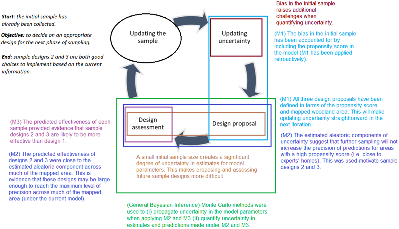
Whilst Bayesian inference offers some natural advantages in adaptive sampling, this alone is not enough to realize all stages of the proposed adaptive sampling architecture. This is because Bayesian inference on its own not offer any insights into how one may design and analyze different sampling practices so that one can best manage the trade-offs between sampling costs and uncertainty. More specifically, in terms of our four key stages, there is still a gap concerning the design proposal and design assessment stages. This section introduces three methods that are designed to implement these stages in our woodland case study: (M1) using predictors in a model as a basis for targeted sampling, (M2) quantifying aleatoric components of uncertainty, and (M3) predicting the effects of different sampling. The interactions between the key stages and these methods are summarized in Figure 4, and a guided example is provided in Appendix Section A.3.
A summation diagram of how Bayesian inference and methods (M1–M3) interact with the four key stages of adaptive sampling.

3.3.1. M1: Using predictors in a model as a basis for targeted sampling
One key feature of an adaptive sampling approach is that the sampling designs may be different for each of the subsamples and is dependent on the previous subsamples. In general, this can make the quantifying of uncertainty noticeably more difficult. Whilst it is possible to use modeling to account for biased sampling (Winship and Mare, Reference Winship and Mare1992; Cortes et al., Reference Cortes, Mohri, Riley and Rostamizadeh2008), this often requires a large degree of domain knowledge and additional modeling assumptions. For adaptive sampling, this may be unavoidable in initial subsamples as alternative data may not be available at the beginning. For later subsamples though, one may wish to avoid sample designs that require further modeling assumptions, as this can have a detrimental effect on the trust users have in any inferences.
One way to avoid such complications in Bayesian inference is to use only the predictors in a model to define targeted sampling designs in each iteration. As a brief explanation, this is because targeted sampling defined using only the predictors does not alter the likelihood function in any meaningful way (i.e., it only changes the likelihood function up to a constant of proportionality). Hence, the posterior distributions are not changed under this form of targeted sampling. A fuller explanation of this further is given in Appendix Sections A.1 and A.2. The key consequence of this result is that providing the bias in a sample design is some function of the predictors, one can assume the reference data came from a simple random sampling when formulating likelihood functions. This greatly simplifies the problem of formulating likelihood functions from targeted sampling. In addition, one does not need the sample design to be explicitly stated, which becomes useful when combining multiple subsamples with different designs. The reason for this is that if all the subsamples can define their targeting through the model predictors, any bias in their composition is also some function of the predictors. Hence, with Bayesian inference, the updating uncertainty stage can be made easier by defining the design of each subsample through the predictors as one does not need to make any additional adjustments to infer the likelihood function at each iteration. This result can also be used as a simple way of including subsamples that are biased with respect to some propensity scoring by having the model include these propensity scores as predictors (Angrist, Reference Angrist1997). This becomes important when there are different costs associated with collecting true values that vary across a population.
The idea of using the predictors in a model to define targeted sampling is also important in the design proposal stage of an adaptive sampling strategy when it is applied alongside other methods. The idea here is that one can use alternative methods (e.g., analyzing aleatoric components of uncertainty in M2) to identify members of a population that one would prefer to target for efficiency reasons and then define a sample design through the predictors to target these members. Effectively, this type of approach offers a way for creating efficient sampling designs that preemptively make updating uncertainty a less complicated task in the next iteration.
3.3.2. M2: Quantifying aleatoric components of uncertainty
The aleatoric component of uncertainty is a means of quantifying the precision of predictions should all the components in a model be known (i.e., when there is no uncertainty propagating from the parameter or input values) (Hüllermeier and Waegeman, Reference Hüllermeier and Waegeman2021). This acts as a way of measuring the limit to which further sampling alone increases the precision of predicted values (in the current modeling system). In practice, the level of aleatoric uncertainty is often represented as stochastic elements in a model. However, the exact degree of aleatoric uncertainty will likely be unknown, as these stochastic elements of uncertainty will often be dependent on unknown model parameters.
With Bayesian inference, one can account for the uncertainty in an aleatoric component of uncertainty by applying a specific form of model chaining. For example, the aleatoric variance is simply the variance in a prediction should all the components in a model be known. By comparing the aleatoric component of uncertainty to the current level of precision in a prediction, one can gauge the likely benefit further sampling may bring to increasing the precision in a prediction. For example, if this difference is minimal, this is an indication that any further sampling is likely to have little effect in increasing the precision. At this point, one must consider alternative models to increase the precision of predictions.
Quantifying aleatoric components of uncertainty can be useful firstly in the design proposal stage of an adaptive sampling strategy. This is because it can indicate which members of a population a sample may want to avoid targeting, as one is unlikely to see a significant increase in the precision of the predictions in these areas unless the model itself is changed. Secondly, it is useful in the design assessment stage as it can give users an indication of when to stop collecting subsamples and this also aids in comparing the effectiveness of different proposed sampling designs by setting a baseline.
3.3.3. M3: Predicting the likely effects of further sampling
Under Bayesian inference, it is possible to predict the effectiveness of a proposed design for a future subsample given the current data. This is done by viewing this problem as a specific form of generating a posterior distribution in model chaining, where the unknown value is some measure of the precision in a prediction after the proposed subsample has been collected and combined with the original data. Predicting the effects of further sampling is a useful tool in the design assessment stage as it allows one to compare the likely effectiveness of multiple proposal designs sample without needing to implement them (Phillipson et al., Reference Phillipson, Blair and Henrys2019).
Predicting the likely effects of further sampling is important as often one will need to decide between a shortlist of sample designs. This is because it is not always easy to provide a single optimal sample design as (a) the true parameter values are usually unknown, and (b) there is often a trade-off to manage between the cost of a sample and the likely gain in precision for an estimate.
The ability to predict the likely effects of further sampling is expected to work well in combination with M2 as the aleatoric component of uncertainty can help contextualize the results of this analysis by providing an estimate for the maximum level of precision.
4. Evaluation Using the Woodland Case Study
In this section, the methods presented in Section 3 are evaluated for how they can assist in realizing the key stages of adaptive sampling through the woodland mapping problem introduced in Section 2. Here, the methods are evaluated on two criteria:
-
• How do these methods help in overcoming the challenges in this case study?
-
• How easily could these methods be applied to similar mapping problems?
The first criterion is based on the premise that this case study is representative of common challenges seen in reference sampling (see Section 2 for further details). Hence, if the proposed methods can help in realizing the key stages of adaptive sampling in this case study, this is an early indication that such methods will benefit general applications. The second criterion is designed to act as a more explicit consideration of generalizability.
In terms of the four key stages, the case study begins at the point where the initial sample has been collected (i.e., it begins just after the updating the sample stage has been completed). The objective here is to get to a point where one can decide on an appropriate design for the next phase of sampling. However, the initial sample is both biased and modest in size, this has created several challenges across the stages (this is summarized in Figure 5).
A summation of how the features in the woodland case study create challenges across the four key stages of adaptive sampling.

Firstly, the bias in the initial sample raises additional challenges when updating the uncertainty. Many methods of quantifying uncertainty rely on formulating probabilistic statements based on a sample design and observed data. Typically, this is harder to do under biased sampling when compared to less complex sample designs (e.g., simple random sampling). Secondly, a small initial sample size creates a significant degree of uncertainty in estimates for model parameters. This makes proposing and assessing future sample designs more difficult as many methods at these stages are dependent on the true parameter values.
4.1. Updating the uncertainty with a biased sample
The first task here is to move past the updating uncertainty stage. Here, a model for the ground truth values is created using the mapped woodland values as we suspect that this is a strong predictive feature of the ground truth values. Because of the initial bias in the sample though, one cannot fit a model that makes use of only ground truth values with this data (without some relying on heavy modeling assumptions).
As the bias in the initial sample design is known to be dependent only on the propensity score, this issue can be dealt with by including the proximity score as an input feature in any model. This is effectively M1 applied retroactively. Note that this does not restrict which other features can be included in the model. Namely, one is still free to include the mapped woodland as an input in the model.
A model based on Bayesian kernel machine regression (Bobb et al., Reference Bobb, Valeri, Henn, Christiani, Wright, Mazumdar, Godleski and Coull2014) using the propensity score and mapped woodland features as model inputs have been chosen in this case as the kernel-based nature of the model provides a lot of flexibility for the trends between the model inputs and outputs. This allows the data to “speak for itself” more and lessens the need for users to define rigid model structures that may not be appropriate. This can be a desirable property in the early stages of adaptive sampling as may be hard to justify rigid model statues on initial samples that may be modest in size (which in turn can make the model inaccurate).
With this, one can apply standard model fitting procedures to create to quantify the uncertainty in the ground truth woodland area. This can be viewed across the feature space (Figure 6).
A Bayesian kernel machine regression (bkmr) model fitted to the initial sample.

As a side note, there are many alternative models with flexible structures one could have used (e.g., generalized additive models [Wood, Reference Wood2017] and Gaussian process models [Shi et al., Reference Shi, Murray-Smith and Titterington2003]) and models that consider spatial auto-correlation structures (Dormann et al., Reference Dormann, McPherson, Araújo, Bivand, Bolliger, Carl, Davies, Hirzel, Jetz, Kissling, Kühn, Ohlemüller, Peres-Neto, Reineking, Schröder, Schurr and Wilson2007). In general, is it good practice to assess the sensitivity of model choice when one is unsure which model to choose. This is discussed further in Section 5.
4.2. Proposing sample designs under uncertainty
The next phase is to move on to the design proposal and design assessment stages. The aim here is to generate a sample design that is likely to increase the precision of the model efficiently. This begins by adding the restriction that any proposed sample designs must define any targeting using only the mapped woodland and propensity score features. With this restriction, including this new data into the model fit is a simple task, as no additional modeling assumptions are required. Effectively, M1 is applied once more as a preemptive measure to ensure updating the uncertainty stage straightforward in the next iteration.
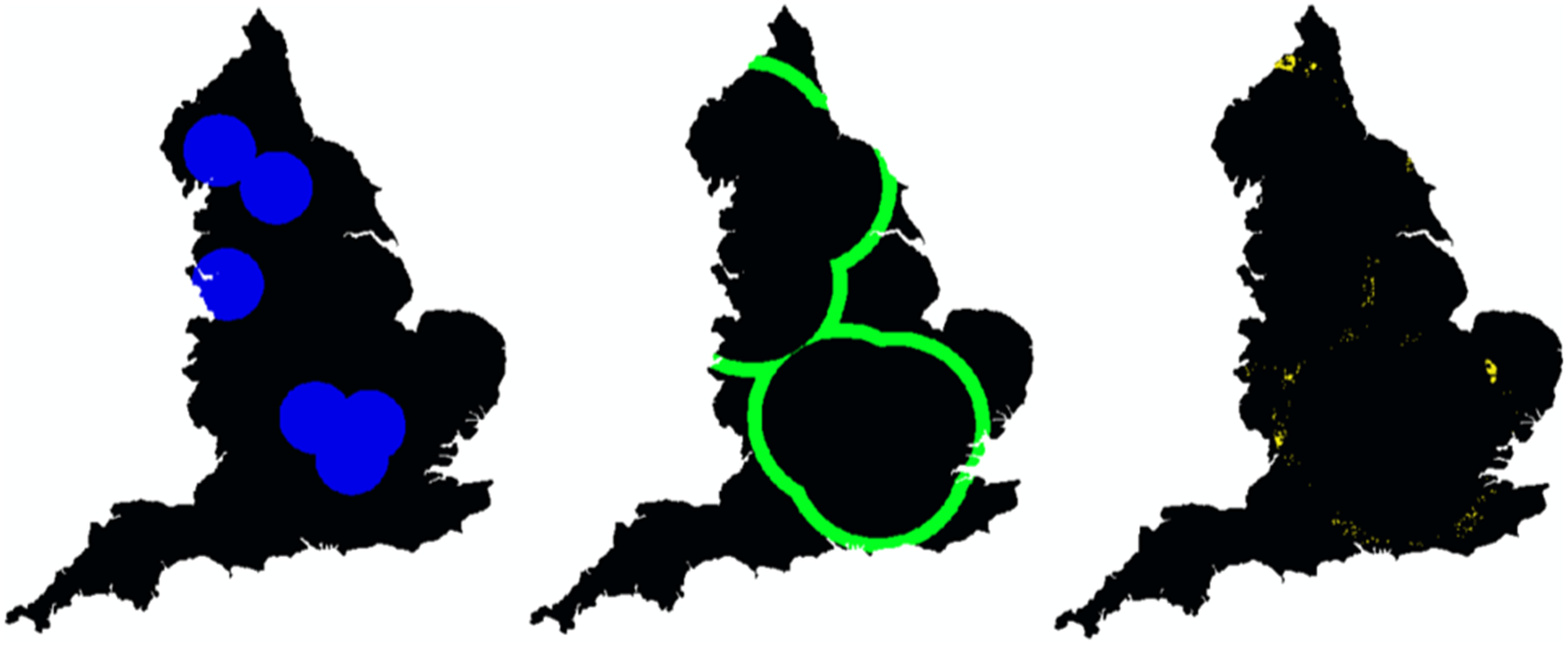
With this restriction added, one now needs to determine where designs should target to reduce uncertainty efficiently. In this case, one can use M2 to guide for sample designs sample for the woodland area predictions across each of the 1 km squares. The precision of any estimate or prediction is measured using the standard deviation of its posterior distribution. By comparing the current levels of precision in the predictions with its (estimated) aleatoric standard deviation, one can identify areas that are likely to be close to their maximum level of precision (under the current model). From Figure 7, one can see that, for areas within or close to the initial sampling area (a), the current level of precision (b) is similar to the aleatoric component of uncertainty (c). This is an indication that further sampling should look toward targeting locations that are further away from the experts’ homes, as any further sampling design is unlikely to increase the precision for predictions in these areas.
(a) A map of the target area for the initial sample. (b) A map of the current level of precision for woodland area predictions. (c) A map for the estimated aleatoric component of uncertainty, a measure of the maximum level of precision for predictions under this model.

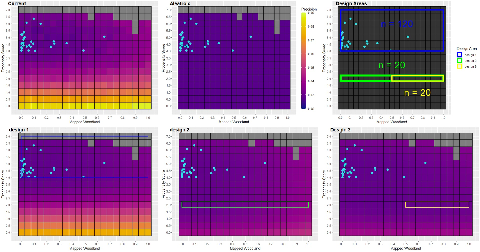
An additional way to analyze components of uncertainty is to visualize them across the model input space. This can be useful when looking to formally define sample designs as targeting areas in this space allows one to make use of M2 to easily update the model afterward. From Figures 8 and 9, one can see that, as the proximity scores decrease, the current level of precision begins to increase sharply. The precision of predictions in these areas is well above the estimated aleatoric component. Using this analysis as a heuristic guide, there is a strong indication that one may need to venture out to areas with a low propensity score to see any meaningful increase in the prediction of the estimates outside of our original sampling areas.
Measures of precision across the predictive features via heat maps. The light-blue points indicate the initial sample.

Measures of precision across the predictive features in 3D space (mapped woodland and propensity score). The black surface represents the current level of precision. The red surfaces represent estimates for the aleatoric components (posterior mode and 95% credible surfaces).

4.3. Design assessment under uncertainty
Whilst it may not be possible to generate specific sample designs with M3, one can still predict the likely effects sample designs will have on the precision of the predictions. Furthermore, one can account for the uncertainty that comes from using the initial sample to estimate model parameters by using Monte Carlo methods. This allows for a try-before-you-buy approach for assessing different sample designs, which can then be used to generate efficient designs through exploration and experimentation.
In this case study, three possible designs are considered:
-
• Design 1 (blue): A larger-sized sample (120) in the same areas as the initial sample (i.e., a propensity score greater than or equal to 4). This design has been selected to examine the hypothesis that there is little to be gained when sampling from this area alone and that venturing out into further areas will be necessary.
-
• Design 2 (green): A modest-sized sample (20) targeting propensity score greater than 1.8 but less than 2.2. This design has been chosen to consider the possibility of experts visiting further away areas. Because of the COVID restriction on staying overnight, visiting a large number of sites in these areas may not be possible.
-
• Design 3 (yellow): A modest-sized sample (20) of a mapped woodland area of more 0.5 than and propensity score greater than 1.8 but less than 2.2. This is similar to design 2, except it also restricts sampling to areas that have a higher mapped woodland value. This design is chosen to take into account that woodland areas are relatively rare in the mapping.
Figure 10 shows each of the targeted areas for each design across the England mapping. Note that, since all three sample designs are defined in terms of the propensity score and the mapped woodland values, one can easily update the posterior distributions using M1.
Spatial mappings for the targeted areas under each sample design (design 1: blue, design 2: green, design 3: yellow).
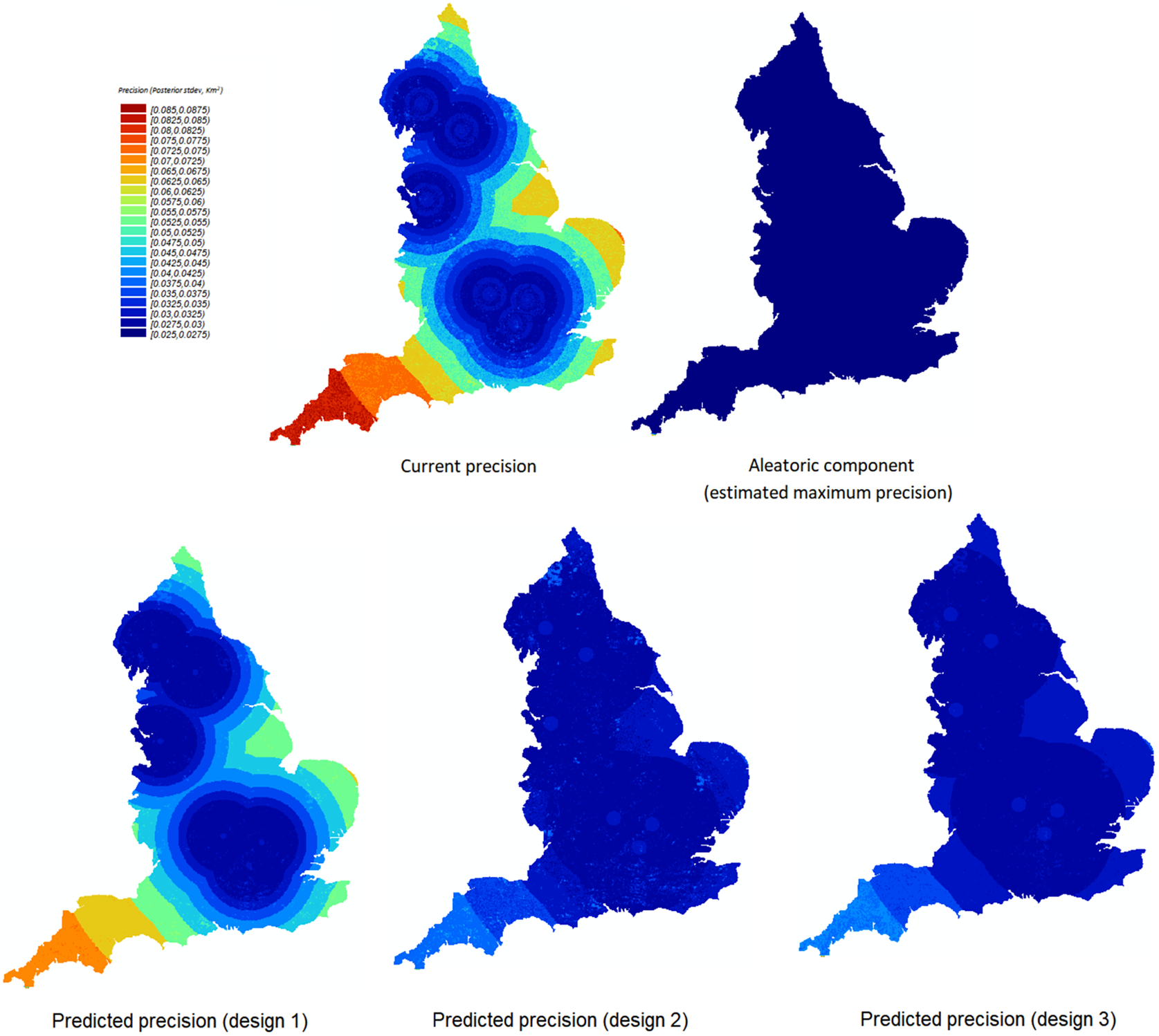
With M3, the expected effects each sample design will have on the precision of the estimates can then be compared. From Figures 11−13, one can observe the following:
-
• Design 1 is likely to have little impact on the precision of the predictions when compared to the current precision using the initial sample alone.
-
• Design 2 and design 3 are likely to be more effective than design 1 for increasing the precision of the predictions of the woodland area within these 1 km squares.
-
• The predicted precision under design 2 and design 3 is close to the aleatoric standard deviation for a large area of the map. This suggests that for a significant proportion of the map, there is a good chance that sample designs 2 and 3 will be enough to achieve the maximum possible precision (under this model) for predictions of woodland extent.
-
• The differences in likely impacts between designs 2 and 3 are minor across the map, so it is not as clear which will be more effective for increasing the precision of the predictions at this stage.
The predicted precision for woodland area predictions under the three proposed sample designs presented spatially.
The predicted precision for woodland area predictions under the three proposed sample designs across the predictive features via heat maps. The light-blue points indicate the initial sample and the colored rectangles display the target areas for the proposed sample designs.
The predicted precision for woodland area predictions under the three proposed sample designs was presented across the predictive features in 3D space (mapped woodland and propensity score).

From a decision-making perspective, these observations suggest that firstly, it would be better to venture further away from where the surveyors are based and apply designs such as 2 or 3, even if it comes at the expense of a smaller sample size. Secondly, they suggest that it may be best to apply sample designs such as design 2 or design 3 (and then perform a second iteration of adaptive sampling) before committing to designs with larger sizes. This is because there is a strong possibility that the additional reference data from these modestly sized samples will be enough for a significant proportion of the map. Hence, by applying one of these modestly sized samples first, one then can lessen the risk of wasting resources on unnecessary reference data.
As an aside, it may be difficult to distinguish between design 2 and design 3 based solely on their ability to increase the precision in predictions at this stage. However, there may be other factors to consider from a practical perspective. For example, the spatial clustering in design 3 can be convenient when physically visiting areas to obtain ground truths. On the other hand, the fact that design 2 is defined using only the propensity score can be an advantage when using the reference data to fit other models (e.g., for other classes), as one is free to apply M1 without needing to include the mapped woodland in the model.
4.4. Evaluation
Overall, the case study has illustrated the significant benefits of our proposed approach. Within the case study (see Figure 14 for a full summary) one was able to see that by using the propensity score as a predictor in a model, one can include the targeted initial sample without needing to rely on heavy assumptions (e.g., that the targeted area is representative of the wider mapping area). These principles were used again when constructing the three proposal sample designs. For each design, one could combine the reference data from these samples with the initial sample without needing to make any additional assumptions or corrections when updating the uncertainty.
A summation of how the features in the woodland case study create challenges across the four key stages of adaptive sampling and how methods M1–M3 help in overcoming them.
Furthermore, by considering the aleatoric component of uncertainty in the predictions, one could estimate a maximum level of precision. This acted as a useful guide for proposing sample designs and allowed us to contextualize some of the results when predicting the likely effects of further sampling under different designs. By taking a Bayesian approach, one could predict the likely effects of different sample designs with Monte Carlo methods. From an adaptive sampling perspective, these methods allowed us to propose cost-effective designs for further sampling and analyze their likely effects based on the information from a small and biased initial sample.
From a more general perceptive, the idea of using propensity scores within models, as a means of accounting for purposely biased or targeted sampling, can easily be extended to other applications. This is because one can change the factors defining a propensity score without changing the core methodology. For example, one could easily replace the propensity score in the case study with one that uses a more sophisticated assessing the accessibility of the area (e.g., a score that considers the distance from roads and elevation)
Another important property of the proposed approach is that, once the propensity scores are included, one does not need to make any alterations to any likelihood functions to account for any biases defined through such scores. This allows us to use third-party modeling tools as including an extra feature in a model is often much easier than redefining or editing likelihood functions. This property is vital in the case study when using the bkmr (Bobb, Reference Bobb2017) package in R to fit the models.
Predicting the likely effects of further sampling under Bayesian inference can also be brought into other mapping applications and models with little additional work. The main reason for this is that with Bayesian inference, one can make use of Monte Carlo methods when quantifying uncertainty. Monte Carlo methods are highly generalizable. All that is required here is that one can (a) draw from a posterior distribution for a model’s parameters under a given set of reference data, and (b) simulate drawing samples from a model under fixed parameters values.
However, there are several limitations to note from the methods used in this case study. Firstly, the idea of using propensity scores in models to avoid problems with sample bias requires that one can explicitly state the factors that bias a sample. This is not an issue if the propensity is predefined (e.g., based on the known costs or preferences), but this does become an issue when using reference data in which the sampling is not strictly controlled (e.g., relying on opportunistic data).
Secondly, there are still major gaps in terms of the availability of suitable methods for proposing sample designs. In this case study, the aleatoric components were used to act as a guide for sample designs. Ideally, one would want methods that can give explicit recommendations on the sizes of future subsamples or where they should target (possibly under some cost constraints).
Thirdly, Monte Carlo methods can be computationally expensive, and this can become a problem when dealing with higher-resolution imagery or when predicting the effects of many proposed sample designs. In this case study, one was forced to compromise on this by only considering three proposal designs and approximating their effects by considering a grid of discrete points across our feature space.
5. Discussion
This paper has identified some opportunities, but also some challenges that come from applying adaptive sampling to mapping problems. From this, the paper has demonstrated how many of these challenges can be overcome by using methods based on Bayesian inference. At its heart, adaptive sampling is intended to be a decision-making tool that is used by practitioners to better manage any cost-benefit trade-offs when collecting reference data. This section discusses two areas with the potential to take this further.
5.1. Combining adaptive sampling and adaptive modeling
One area in which this framework could be taken further would be to incorporate situations where there may be multiple plausible models. In this paper’s case study, one considered how different sample designs may affect the precision of predictions under a fixed model. With any model-based approach though, there is also uncertainty in the choice of model and the suitability of assumptions made in the said model. Often, there is a balancing act between the appropriate level of structure in a model, the accuracy of the model, and the precision of predictions. This is especially relevant when sample sizes are limited by cost constraints. This is because one often needs a sizeable amount of reference data before models with more generalized structures are precise enough to be practically viable.
One option here would be to consider a shortlist of models and see where they agree and where they disagree across a mapping. In this situation, areas with a large validation between the models’ predictions would be an indication that future sampling should target these areas. Furthermore, some models may be added and removed from the shortlist as more reference data becomes available. The generalizability of Monte Carlo methods would help in these situations, as the core methodology is the same across models.
An alternative approach is to combine shortlisted models into one model through an ensemble approach. For example, one could consider a weighted average of multiple models. Bayesian inference is naturally suited to this, as the weights can easily be included as another model parameter and hence considered in posterior distributions (Monteith et al., Reference Monteith, Carroll, Seppi and Martinez2011). This could act as a more automated (and less abrupt) way of adding and removing or adding models as more reference data is collected.
5.2. Creating an environment that allows for easy design experimentation
Another area in which this framework could be taken further would be to develop a means of allowing users to easily propose, assess and potentially alter sample designs. The motivation behind this begins with observing that the problem of proposing efficient sample designs in mapping applications is extremely complex. This is further compounded by the fact that there is often no single correct or optimal sample design, but rather a series of trade-offs between designs. This makes the idea of providing practitioners with an explicit set of instructions for generating efficient sample designs (e.g., by viewing it as an optimization problem) seem infeasible in practice. Hence, we suggest focusing on giving practitioners the means to explore different sample designs, so that they are best able to judge the potential trade-offs within their given context. In short, it is less about telling practitioners where they should be sampling and more about giving them the tools to discover this for themselves.
However, some methods presented in this paper (M3 in particular) can be computationally expensive when relying on Monte Carlo methods. This is can make exploring different sample designs (and potentially different models) difficult as generating any results for each scenario can take a long time. A secondary challenge is that these methods require a degree of technical expertise to initially set up. Overcoming these challenges is not impossible (e.g., investing in computational infrastructure and hiring staff familiar with Bayesian inference) but doing so can a significant upfront cost to adaptive sampling. This is not ideal, given the main motivation behind adaptive sampling is to act as a cost-effective way of collecting reference data.
With this in mind, one could consider cloud-based systems as a means of providing a service that gives users the tools to investigate different combinations of models and sample designs. This approach has seen recent success in mapping applications (Cope et al., Reference Cope, Mikhailova, Post, Schlautman and McMillan2017; Nourjou and Hashemipour, Reference Nourjou and Hashemipour2017; Mariushko et al., Reference Mariushko, Pashchenko and Nechausov2018; Sousa et al., Reference Sousa, Fatoyinbo, Neigh, Boucka, Angoue and Larsen2020). One potential advantage of cloud-based systems is that they can avoid the previously discussed challenges related to computational and expertise costs as these problems that are not put on to the users.
6. Conclusion
In the recent decade, there has become a growing trend of using a combination of satellite imagery data and MLTs to generate mappings quickly and cheaply. Nevertheless, it is still important that one collects a sample of reference data to quantify the uncertainty in any predictions made using these mappings. However, because collecting reference data can be expensive, one must carefully consider the cost-to-benefit trade-offs in any sample design when collecting this reference data.
This paper investigated how a combination of adaptive sampling and methods based on Bayesian inference could be used in mapping applications to offer a generalizable way of managing trade-offs when considering sample designs. The discussion was based around a real-world case study and, within this case study, one was faced with two significant challenges: (a) the initial sample was biased due to COVID-19 travel restrictions; and (b) the initial sample was small in size (thereby adding uncertainty to any initial estimates). From this case study, we identified the following:
-
• A key component of adaptive sampling is the need to quantify uncertainty using data collected under sampling bias. This bias can be a consequence of deliberate targeting or because of practical constraints. In either case, if the sample bias can be expressed as a propensity score, then such bias can be automatically accounted for by including this propensity score as a predictive feature in any model. This result becomes especially important when considering multiple iterations of sampling, as it allows users to forego complicated (and often assumption-heavy) bias-correction methods between iterations.
-
• Overall, many processes and methods used for adaptive sampling are made significantly easier with Bayesian inference. This case study included quantifying uncertainty when samples are collected sequentially, estimating the maximum level of precision in predictions, and predicting the effects of different sample designs. Furthermore, one easily accounts for the uncertainty in initial estimates under Bayesian inference with Monte Carlo methods allowing for more robust analysis when decision-making. This is especially useful in the early stages of adaptive sampling when the current sample is small in size.
-
• The findings from this case study are highly relevant to other mapping applications. This is because many of the methods investigated in this case study did not rely on the specific choice of models or propensity scores.
Future work in this area would be to go from the current state of adaptive sampling (a collection of useful methods) to a usable decision-making tool where practitioners can better manage any cost-benefit trade-offs when collecting reference data. Two specific areas here include: (a) accounting for the fact that there may be many plausible models when quantifying uncertainty from reference data and that the choice of a model may need to change throughout adaptive sampling (i.e., combining sampling with adaptive modeling); (b) developing a platform in which users can easily to propose, assess and alter sample designs and models for themselves.
Data Availability Statement
The original 2007 land cover map (LCM 2007) can be found at: Morton et al. (Reference Morton, Rowland, Wood, Meek, Marston and Smith2014). The survey data used for the reference data can be found at: Brown et al. (Reference Brown, Bunce, Carey, Chandler, Crowe, Maskell, Norton, Scott, Scott, Smart, Stuart, Wood and Wright2016). The R code used for the case study and example in Appendix Section A.3 can be found at: https://zenodo.org/badge/latestdoi/508823025.
Competing Interests
The authors declare no competing interests exist.
Author Contributions
Conceptualization: J.P.; Data curation: P.H.; Methodology: J.P.; Software: J.P.; Writing—original draft preparation: J.P., G.B., P.H.; Writing—reviewing and editing: G.B., P.H.
Funding Statement
This work is supported by the following grant: DT/LWEC Senior Fellowship in the Role of Digital Technology in Understanding, Mitigating, and Adapting to Environmental Change, EPSRC: EP/P002285/1.
Ethics Statement
The research meets all ethical guidelines, including adherence to the legal requirements of the study country.
A. Appendix
In the introduction of M1 in Section 3, it was claimed that providing the bias in a sample design can be expressed entirely through the predictive features, and that one can treat the reference data as though it came from simple random sampling when formulating likelihood functions. It was further claimed that this result in turn makes updating uncertainty in Bayesian inference significantly easier. This section discusses the importance of this result when quantifying uncertainty through case Bayesian inference and then goes on to show the result.
A.1. The importance of similar likelihood functions when quantifying uncertainty with Bayesian inference
Suppose the relationship between an outcome y and predictors $ x $
is represented through a model f with
$ x $
is represented through a model f with $ y\hskip0.35em =\hskip0.35em f\left(x;\theta \right) $
, where
$ y\hskip0.35em =\hskip0.35em f\left(x;\theta \right) $
, where $ \theta $
denotes a set of unknown parameters.
$ \theta $
denotes a set of unknown parameters.
Under Bayesian inference, one can use a sample obtained under design $ S $
, which consists of predictors
$ S $
, which consists of predictors $ X $
and associated outcomes
$ X $
and associated outcomes $ Y $
, to generate a posterior distribution for
$ Y $
, to generate a posterior distribution for $ \theta $
with
$ \theta $
with
 $$ \pi \left(\theta |D,S\right)\propto \pi \left(D|\theta, S\right)\pi \left(\theta |S\right), $$
where $ \pi \left(D|\theta, S\right) $
denotes the likelihood of observing data
$ \pi \left(D|\theta, S\right) $
denotes the likelihood of observing data $ D\hskip0.35em =\hskip0.35em \left(X,Y\right) $
under a sample design
$ D\hskip0.35em =\hskip0.35em \left(X,Y\right) $
under a sample design $ S $
conditional on
$ S $
conditional on $ \theta $
. This is the probability of observing
$ \theta $
. This is the probability of observing $ D $
obtained under a sample design
$ D $
obtained under a sample design $ S $
for a fixed value of
$ S $
for a fixed value of $ \theta $
.
$ \theta $
. $ \pi \left(\theta |S\right) $
is the prior distribution on
$ \pi \left(\theta |S\right) $
is the prior distribution on $ \theta $
given
$ \theta $
given $ S $
. This is a representation of the prior knowledge of
$ S $
. This is a representation of the prior knowledge of $ \theta $
given S. represented as a probability density function.
$ \theta $
given S. represented as a probability density function.
For the sake of simplification, one can assume $ \theta $
is independent of
$ \theta $
is independent of $ S $
, that is,
$ S $
, that is, $ \pi \left(\theta |S\right)\hskip0.35em =\hskip0.35em \pi \left(\theta \right) $
, without much loss of generality. This is because the only way for the converse to hold (i.e., the prior knowledge of
$ \pi \left(\theta |S\right)\hskip0.35em =\hskip0.35em \pi \left(\theta \right) $
, without much loss of generality. This is because the only way for the converse to hold (i.e., the prior knowledge of $ \theta $
is dependent on the sample design) is if the design of a sample not yet implemented influences the prior belief in
$ \theta $
is dependent on the sample design) is if the design of a sample not yet implemented influences the prior belief in $ \theta $
, which is absurd in most reasonable applications. With this additional minor restriction, one has
$ \theta $
, which is absurd in most reasonable applications. With this additional minor restriction, one has
 $$ \pi \left(\theta |D,S\right)\propto \pi \left(D|\theta, S\right)\pi \left(\theta \right), $$
From (A.2), one can see that the only point where this posterior distribution is influenced by the sample design of the observed data is in the likelihood function. This means that under a fixed prior $ \pi \left(\theta \right) $
, one has
$ \pi \left(\theta \right) $
, one has
 $$ \pi (D|\theta, \hskip2pt S)\propto \pi (D|\theta )\Rightarrow \pi (\theta |D,\hskip2pt S)\hskip0.35em =\hskip0.35em \pi (\theta |D). $$
In other words, if the likelihood functions under two different sample designs are proportional to each other, then any uncertainty in the model parameters (as quantified by a posterior distribution under a fixed prior) will be the same. From this, it is easy to show (by considering distributions conditioned on $ Y $
) that this result can be used to extend this idea to include uncertainty in estimates that are functions of any outcomes.
$ Y $
) that this result can be used to extend this idea to include uncertainty in estimates that are functions of any outcomes.
 $$ \pi (D|\theta, \hskip2pt S)\propto \pi (D|\theta )\Rightarrow \pi (g({y}^{\ast })|{x}^{\ast },\hskip2pt D,\hskip2pt S)\hskip0.35em =\hskip0.35em \pi (g({y}^{\ast })|{x}^{\ast },\hskip2pt D), $$
where $ {x}^{\ast } $
represents the predictors for some outcome
$ {x}^{\ast } $
represents the predictors for some outcome $ {y}^{\ast}\hskip0.35em =\hskip0.35em f\left({x}^{\ast };\theta \right) $
.
$ {y}^{\ast}\hskip0.35em =\hskip0.35em f\left({x}^{\ast };\theta \right) $
.
The reason this result is important is that some well-known results related to conjugate priors and most statistical software packages will implicitly assume a simple random sample design when generating posterior distributions. Results such as (A.3) and (A.4) demonstrate that if one can show that if a sample design leads to a likelihood that is proportional to the likelihood function generated under simple random sampling, then one can use these results and third-party software without the need to make any adjustments. This is a major advantage, as it allows a user to simply input any reference data into preexisting methods, which have already been developed and potentially optimized. Developing bespoke equivalents for different sample designs is theoretically possible, but can come with significant computational and expertise costs and may rely on additional modeling assumptions to implement.
A.2. Targeted sampling defined through predictors: why this leads to likelihood functions similar to simple random sampling
The idea behind M1 in the main part of this paper is that any design $ S $
defined through the predictors in a model, will be enough to meet (A.3) and (A.4). Here, we formalize this idea and show the result.
$ S $
defined through the predictors in a model, will be enough to meet (A.3) and (A.4). Here, we formalize this idea and show the result.
Claim: Let $ I $
denote a subset of a population and
$ I $
denote a subset of a population and $ S $
denote some sample design. Next, let
$ S $
denote some sample design. Next, let $ D(I)\hskip0.35em =\hskip0.35em \left(Y(I),X(I)\right) $
, where
$ D(I)\hskip0.35em =\hskip0.35em \left(Y(I),X(I)\right) $
, where $ Y(I) $
,
$ Y(I) $
, $ X(I) $
denotes the outcomes and predictors under model with parameters
$ X(I) $
denotes the outcomes and predictors under model with parameters $ \theta $
for the members of the population contained in
$ \theta $
for the members of the population contained in $ I $
respectively. If there exists a
$ I $
respectively. If there exists a $ g $
such that
$ g $
such that $ \pi \left(I|S\right)\hskip0.35em =\hskip0.35em g(X) $
then
$ \pi \left(I|S\right)\hskip0.35em =\hskip0.35em g(X) $
then $ \pi \left(\theta |D,S\right)\hskip0.35em =\hskip0.35em \pi \left(\theta |D\right) $
.
$ \pi \left(\theta |D,S\right)\hskip0.35em =\hskip0.35em \pi \left(\theta |D\right) $
.
Proof: Let $ S $
be sample design such that
$ S $
be sample design such that $ \pi \left(I|S\right)\hskip0.35em =\hskip0.35em g(X) $
. Next, one can consider considering two equivalent expressions for the joint probability distribution,
$ \pi \left(I|S\right)\hskip0.35em =\hskip0.35em g(X) $
. Next, one can consider considering two equivalent expressions for the joint probability distribution, $ \pi \left(D,S|\theta \right) $
In the first case, one has
 $$ \pi \left(D,S|\theta \right)\hskip0.35em =\hskip0.35em \pi \left(S|D,\theta \right)\pi \left(D|\theta \right), $$
which comes from the definition of a conditional distribution and is true for any $ S $
$ S $
From this, one can make use of the condition that $ \pi \left(I|S\right)\hskip0.35em =\hskip0.35em g(X) $
. Here,
$ \pi \left(I|S\right)\hskip0.35em =\hskip0.35em g(X) $
. Here, $ \pi \left(I|S\right)\hskip0.35em =\hskip0.35em g(X) $
implies that
$ \pi \left(I|S\right)\hskip0.35em =\hskip0.35em g(X) $
implies that $ \pi \left(S|D,\theta \right)\hskip0.35em =\hskip0.35em \pi \left(S|X\right) $
as if
$ \pi \left(S|D,\theta \right)\hskip0.35em =\hskip0.35em \pi \left(S|X\right) $
as if $ X $
is known, all other information is redundant when determining the likelihood that the data was sampled under
$ X $
is known, all other information is redundant when determining the likelihood that the data was sampled under $ S $
. This gives one form to the joint probability distribution as
$ S $
. This gives one form to the joint probability distribution as
 $$ \pi \left(D,S|\theta \right)\hskip0.35em =\hskip0.35em \pi \left(S|X\right)\pi \left(D|\theta \right). $$
The second form for $ \pi \left(D,S|\theta \right) $
can be given by first conditioning on the
$ \pi \left(D,S|\theta \right) $
can be given by first conditioning on the $ S $
to give
$ S $
to give
 $$ \pi (D,\hskip2pt S|\theta )\hskip0.35em =\hskip0.35em \pi (D|\theta, \hskip2pt S)\pi (S|\theta ). $$
Since the design of S is determined only by $ X $
, the likelihood of
$ X $
, the likelihood of $ S $
is unaffected by
$ S $
is unaffected by $ \theta $
. This gives
$ \theta $
. This gives $ \pi \left(S|\theta \right)\hskip0.35em =\hskip0.35em \pi (S) $
. Hence the second expression for
$ \pi \left(S|\theta \right)\hskip0.35em =\hskip0.35em \pi (S) $
. Hence the second expression for $ \pi \left(D,S|\theta \right) $
becomes
$ \pi \left(D,S|\theta \right) $
becomes
 $$ \pi \left(D,S|\theta \right)\hskip0.35em =\hskip0.35em \pi \left(D|\theta, S\right)\pi (S). $$
Comparing the right-hand sides of (A.7) and (A.8) yields
 $$ \pi (D|\theta, \hskip2pt S)\hskip0.35em =\hskip0.35em \frac{\pi (S|X)}{\pi (S)}\hskip0.24em \pi (D|\theta )\propto \pi (D|\theta ). $$
The final step is to compare (A.9) with (A.3) to give the desired result.
A.3. Example workflow
Suppose one has a model $ \mathbf{y}\hskip0.35em =\hskip0.35em f\left(\mathbf{x};\theta \right) $
where
$ \mathbf{y}\hskip0.35em =\hskip0.35em f\left(\mathbf{x};\theta \right) $
where $ x $
is a vector of predictors and
$ x $
is a vector of predictors and $ \theta $
denotes a set of parameters. Let
$ \theta $
denotes a set of parameters. Let $ I $
denote a subset of a population,
$ I $
denote a subset of a population, $ S $
denote some sample design, and
$ S $
denote some sample design, and $ D(I)\hskip0.35em =\hskip0.35em \left(Y(I),X(I)\right) $
, where
$ D(I)\hskip0.35em =\hskip0.35em \left(Y(I),X(I)\right) $
, where $ Y(I) $
,
$ Y(I) $
, $ X(I) $
denotes the outcomes and predictors under f for the members of the population contained in
$ X(I) $
denotes the outcomes and predictors under f for the members of the population contained in $ I $
.
$ I $
.
Next, suppose that one wishes to reduce the uncertainty in an unknown quantity $ z\left(\mathbf{y}\right) $
by sampling data of the form
$ z\left(\mathbf{y}\right) $
by sampling data of the form $ D\hskip0.35em =\hskip0.35em \left(Y,X\right) $
using adaptive sampling. Let
$ D\hskip0.35em =\hskip0.35em \left(Y,X\right) $
using adaptive sampling. Let $ U\left(z,D\right) $
denote some measure of uncertainty in
$ U\left(z,D\right) $
denote some measure of uncertainty in $ z $
given data
$ z $
given data $ D $
(e.g.,
$ D $
(e.g., $ U\left(z,D\right)\hskip0.35em =\hskip0.35em v\left(z|D\right) $
, the variance of the posterior distribution for
$ U\left(z,D\right)\hskip0.35em =\hskip0.35em v\left(z|D\right) $
, the variance of the posterior distribution for $ z $
given
$ z $
given $ D $
.
$ D $
.
Under this notation, the combination of the practices introduced in Section 3 can be represented as a workflow described in Table A1, along with a worked example. For the R code accompanying the worked example, see the Data Availability section.
A generalized workflow for the procedures is introduced in Section 3 alongside a worked example.


 Open access