


Impact Statement
Autoregressive models often are aggregated variables from smaller scales. Of particular interest in these models is studying the impact of external perturbations on large-scale variables, which has led to numerous applications across diverse fields. Such studies mainly focus on the effects between the aggregated variables and do not consider the effects between the small-scale variables. Our work presents two contributions. First, we develop a method to quantify the effects of perturbations on small-scale variables within an aggregated autoregressive model. Second, we introduce an approach to provide uncertainty bounds for these effects. Our approach enables the estimation of the effect of an external perturbation at the level of the small-scale variable.
1. Introduction
What are the effects of increased economic activities on air pollution levels? How do different regions of the brain interact and influence one another? Can we accurately estimate the effects of these interactions with a high degree of spatial precision? Understanding the impact of external perturbations on a system is a crucial aspect of dynamic system analysis. However, in fields such as economics and climate science, direct intervention in the system to measure the impact of an external disturbance is often neither feasible nor ethical. Consequently, data-driven approaches are predominantly used to estimate the effects of perturbations on such systems.
In particular, linear time-lagged dependencies between variables are commonly estimated using autoregressive models in neuroscience (Friston, Reference Friston2009), Earth system and climate data analysis (Runge et al., Reference Runge, Bathiany, Bollt, Camps-Valls, Coumou, Deyle, Glymour, Kretschmer, Mahecha, Muñoz-Marí, van Nes, Peters, Quax, Reichstein, Scheffer, Schölkopf, Spirtes, Sugihara, Sun and Zscheischler2019), and macroeconomics (Sims, Reference Sims1980; Zha, Reference Zha, Durlauf and Blume2010). Beyond the estimation of the linear dependencies, the interest often centers on analyzing the effect of an external perturbation on the system. One frequently used quantity to estimate the effects of a shock is, for example, the impulse response. The impulse response indicates the temporal response of an exogenous shock in one of the variables on one or all the other variables. Other measures, such as the accumulated response, reveal the cumulative effect of this shock over several time steps. Finally, the long-run effects (LREs) are the total accumulated effects over all future time steps. In a linear vector autoregressive model (VAR model) (Sims, Reference Sims1980), there are explicit formulas for the impulse response, the accumulated response, and the long-term effects, which can be used to estimate the effect of a shock on the system analyzed (Pesaran and Shin, Reference Pesaran and Shin1998; Lütkepohl, Reference Lütkepohl and Lütkepohl2005). The applications of these explicit formulas are numerous in the literature, especially in macroeconomics. In addition, the estimation uncertainty of these measures can be derived from an asymptotic-based argument or using bootstrapping methods (Benkwitz et al., Reference Benkwitz, Lütkepohl and Wolters2001; Lütkepohl, Reference Lütkepohl and Lütkepohl2005).
To illustrate the range of applications, we give a non-exhaustive list of analyses in which the effects of a perturbation using a VAR model were of interest. In Lütkepohl and Wolters (Reference Lütkepohl and Wolters2003), the authors have investigated the effects of German monetary policy on the monetary sector during the pre-euro period. Blanchard and Perotti (Reference Blanchard and Perotti2002) have studied the effects of a change in government spending and taxes on Gross Domestic Product (GDP) in the United States. More recently, Prüser and Schlösser (Reference Prüser and Schlösser2020) have analyzed the effect of economic policy uncertainty on European economies. In Hayat et al. (Reference Hayat, Ghulam, Batool, Naeem, Ejaz, Spulbar and Birau2021), the relationships between inflation, interest rate, and economic growth have been the main interest. In between macroeconomic, social science, and environmental science, Khan et al. (Reference Khan, Chenggang, Bano and Hussain2020) have examined the relationships between environmental degradation, economic growth, and social well-being in the countries of the Belt and Road Initiative. More focused on public health, Jiang and Liu (Reference Jiang and Liu2022) have analyzed the effect of inflation on infant mortality. Also, in public health, Liu et al. (Reference Liu, Chang and Chen2019) have estimated the effects of economic growth and health progress in the United States. In all of these studies, the variables in the VAR model are often aggregates of smaller-scale variables. In neuroscience, Bullmore and Sporns (Reference Bullmore and Sporns2009) have used the VAR model to study the organization and interaction of different brain regions. In climate science, the interactions between climate indices and modes of variability have been studied. These modes, such as the El Niño–Southern Oscillation (Wunsch, Reference Wunsch1990), the North Atlantic Oscillation (Barnston and Livezey, Reference Barnston and Livezey1987), or the Pacific Decadal Oscillation (Mantua et al., Reference Mantua, Hare, Zhang, Wallace and Francis1997), are the main drivers of global climate from the ocean to stratospheric dynamics. To obtain time series data, modes are extracted from spatially gridded data. While some modes are defined based on expert knowledge, some require the use of dimension-reduction methods such as principal component analysis (PCA) (Storch and Zwiers, Reference Storch and Zwiers1999). The time-lagged dependencies between the modes have been analyzed using various methods (Ebert-Uphoff and Deng, Reference Ebert-Uphoff and Deng2012; Runge et al., Reference Runge, Petoukhov and Kurths2014; Runge et al., Reference Runge, Petoukhov, Donges, Hlinka, Jajcay, Vejmelka, Hartman, Marwan, Paluš and Kurths2015; Kretschmer et al., Reference Kretschmer, Coumou, Donges and Runge2016; Kretschmer et al., Reference Kretschmer, Runge and Coumou2017; Runge et al., Reference Runge, Bathiany, Bollt, Camps-Valls, Coumou, Deyle, Glymour, Kretschmer, Mahecha, Muñoz-Marí, van Nes, Peters, Quax, Reichstein, Scheffer, Schölkopf, Spirtes, Sugihara, Sun and Zscheischler2019; Nowack et al., Reference Nowack, Runge, Eyring and Haigh2020; Galytska et al., Reference Galytska, Weigel, Handorf, Jaiser, Köhler, Runge and Eyring2023; Karmouche et al., Reference Karmouche, Galytska, Runge, Meehl, Phillips, Weigel and Eyring2023).
In the aforementioned fields of study (macroeconomics, public health, environmental science, Earth data analysis, and neuroscience), large-scale variables have commonly been aggregates of smaller-scale variables. This aggregation is mostly spatial (for instance, the climate modes) but can also be an aggregation of individuals, types of products, and so forth (e.g., economic or social indices). Due to the high cross-correlations between small-scale variables and the high dimensionality of the system, it is generally not recommended to model the dependencies between small-scale variables using an autoregressive model. However, some approaches have been developed to overcome this challenge. For example, Yan et al. (Reference Yan, Huang and Genton2021) propose a VAR model where each variable represents a process in a single spatial location. To reduce the high dimensionality of the system, they enforce sparsity and coefficient homogeneity in the transition matrix. To avoid the challenge of high dimensionality, in this study, we take advantage of the time-lagged linear dependencies between large-scale variables, which reveal emergent behavior that coherently appears at the small scale, thereby leading to large-scale dependencies. As a result, we aggregate small-scale variables into large-scale variables whose dependencies can be modeled using an autoregressive model. We use the spatially aggregated VAR (SAVAR) model introduced by Tibau et al. (Reference Tibau, Reimers, Gerhardus, Denzler, Eyring and Runge2022). The SAVAR model was originally designed to benchmark causal discovery methods and was developed for spatial aggregation. In practice, however, the aggregation does not have to be spatial and can be any type of nontemporal aggregation. This model is particularly suited to represent the aggregation of the VAR processes and their linear dependencies due to its matrix of aggregation weights and a single matrix of linear dependencies.
The effects of an external perturbation between large-scale variables can be explicitly calculated using formulas available in the literature. However, the effects of an external perturbation between small-scale variables need to be determined. In addition, approaches for building uncertainty bounds for small-scale effects should also be investigated. Our main contribution is in addressing those two points. We introduce LREs and sensitivity, two measures that indicate the long-term effects of an external perturbation on the small-scale variables. We derive their explicit formulas as functions of the linear coefficients and aggregation weight matrices of an SAVAR model. In addition, we derive the asymptotic distributions of the estimators for these measures under certain assumptions and show how to utilize them for uncertainty quantification. As an illustrative application, we analyze the long-term effects of economic activities on air pollution in Northern Italy, thereby demonstrating the practical utility of our approach in environmental science.
This article is divided into two sections. Section 2 provides a motivational example followed by a detailed description of materials and methods. We briefly introduce the SAVAR model along with relevant notations. We define the sensitivity and the LREs, as two measures that express the long-term effects of a perturbation in an SAVAR model. We derive their explicit formulas as follows. Assuming that the aggregation weights are known and that the underlying VAR process is stable, we derive the asymptotic distributions of their estimators. This asymptotic property can be used to build uncertainty bounds. Section 3 demonstrates the methods through several applications: two experiments with synthetic data and one real-world application. In Experiment 1, we evaluate various methods for estimating the sensitivity using synthetic data. In the second experiment, we analyze different techniques for establishing uncertainty bounds. Specifically, we assess the previously mentioned asymptotic method against multiple bootstrap methods. Finally, in the real-world application, our motivation is to quantify the long-term effects of economic activities on nitrogen dioxide ( $ {\mathrm{NO}}_2 $
) pollution in northern Italy. Our approach allows for estimating these effects at a finer resolution of a spatial grid, rather than the broader resolution of the modeled VAR processes. Additionally, we evaluate the statistical significance of these long-term effects using both bootstrap and asymptotic methods.
$ {\mathrm{NO}}_2 $
) pollution in northern Italy. Our approach allows for estimating these effects at a finer resolution of a spatial grid, rather than the broader resolution of the modeled VAR processes. Additionally, we evaluate the statistical significance of these long-term effects using both bootstrap and asymptotic methods.
2. Materials and methods: Response to a forcing in a linear dynamical system
2.1. Motivating example
In the following, we illustrate the problem of estimating the effects of a particular perturbation in the SAVAR model (Tibau et al., Reference Tibau, Reimers, Gerhardus, Denzler, Eyring and Runge2022) at the level of the small-scale variables. We first present the characteristics of an SAVAR model. In this manuscript, vectors are denoted in bold (e.g., $ \mathbf{y} $
) while scalars remain in regular font.
$ \mathbf{y} $
) while scalars remain in regular font.
Consider, for instance, a set of three VAR processes $ {X}_0,{X}_1,{X}_2 $
that we call modes, as depicted in Figure 1A. The
$ {X}_0,{X}_1,{X}_2 $
that we call modes, as depicted in Figure 1A. The $ {X}_i $
are defined on the small-scale variables
$ {X}_i $
are defined on the small-scale variables $ {y}_j $
stored in a column vector
$ {y}_j $
stored in a column vector $ \mathbf{y} $
so that
$ \mathbf{y} $
so that $ {X}_i={\mathbf{W}}_{\mathbf{i}}^{\prime}\;\mathbf{y} $
where
$ {X}_i={\mathbf{W}}_{\mathbf{i}}^{\prime}\;\mathbf{y} $
where $ {\mathbf{W}}_{\mathbf{i}} $
is a weight vector. A concrete example of such modes is a set of climate modes defined as the weighted average of variables over a grid (temperature, sea level pressure, etc.). In the literature, the estimation of the VAR linear coefficients and the estimation of the effect of a perturbation on one VAR variable on the others are well documented. Diverse measures were derived to study the effect of a perturbation, shock, or impulse in a VAR model, including the impulse response analysis, forecast error variance decomposition, and accumulated response, among others (Pesaran and Shin, Reference Pesaran and Shin1998; Lütkepohl, Reference Lütkepohl and Lütkepohl2005). However, such measures describe the impact at the level of the VAR processes (in Figure 1 the
$ {\mathbf{W}}_{\mathbf{i}} $
is a weight vector. A concrete example of such modes is a set of climate modes defined as the weighted average of variables over a grid (temperature, sea level pressure, etc.). In the literature, the estimation of the VAR linear coefficients and the estimation of the effect of a perturbation on one VAR variable on the others are well documented. Diverse measures were derived to study the effect of a perturbation, shock, or impulse in a VAR model, including the impulse response analysis, forecast error variance decomposition, and accumulated response, among others (Pesaran and Shin, Reference Pesaran and Shin1998; Lütkepohl, Reference Lütkepohl and Lütkepohl2005). However, such measures describe the impact at the level of the VAR processes (in Figure 1 the $ {X}_i $
) and not at the level of the small-scale variables (in Figure 1 the
$ {X}_i $
) and not at the level of the small-scale variables (in Figure 1 the $ \mathbf{y} $
). We think it is also essential to quantify the effects of perturbing one or several small-scale variables on the other small-scale variables in such a model and to provide uncertainty bounds for these effects, as this information is crucial for a thorough understanding of the system’s behavior. We illustrate this problem in Figure 1B. The small-scale variables
$ \mathbf{y} $
). We think it is also essential to quantify the effects of perturbing one or several small-scale variables on the other small-scale variables in such a model and to provide uncertainty bounds for these effects, as this information is crucial for a thorough understanding of the system’s behavior. We illustrate this problem in Figure 1B. The small-scale variables $ \mathbf{y} $
are subject to a particular perturbation, a forcing of intensity
$ \mathbf{y} $
are subject to a particular perturbation, a forcing of intensity $ f $
at time
$ f $
at time $ {t}_0 $
, where we define a forcing as follows:
$ {t}_0 $
, where we define a forcing as follows:
Definition 2.1 (Forcing). A forcing is an external perturbation of intensity $ f $
and weights
$ f $
and weights $ \mathbf{b}\in {\mathrm{\mathbb{R}}}^L $
, as shown in Figure 1B (where
$ \mathbf{b}\in {\mathrm{\mathbb{R}}}^L $
, as shown in Figure 1B (where $ L $
is the total number of grid points). We assume the forcing begins at time
$ L $
is the total number of grid points). We assume the forcing begins at time $ {t}_0 $
and remains constant after that (
$ {t}_0 $
and remains constant after that ( $ t\ge {t}_0 $
), with nonuniform weighting across the grid, specified by
$ t\ge {t}_0 $
), with nonuniform weighting across the grid, specified by $ \mathbf{b} $
.
$ \mathbf{b} $
.
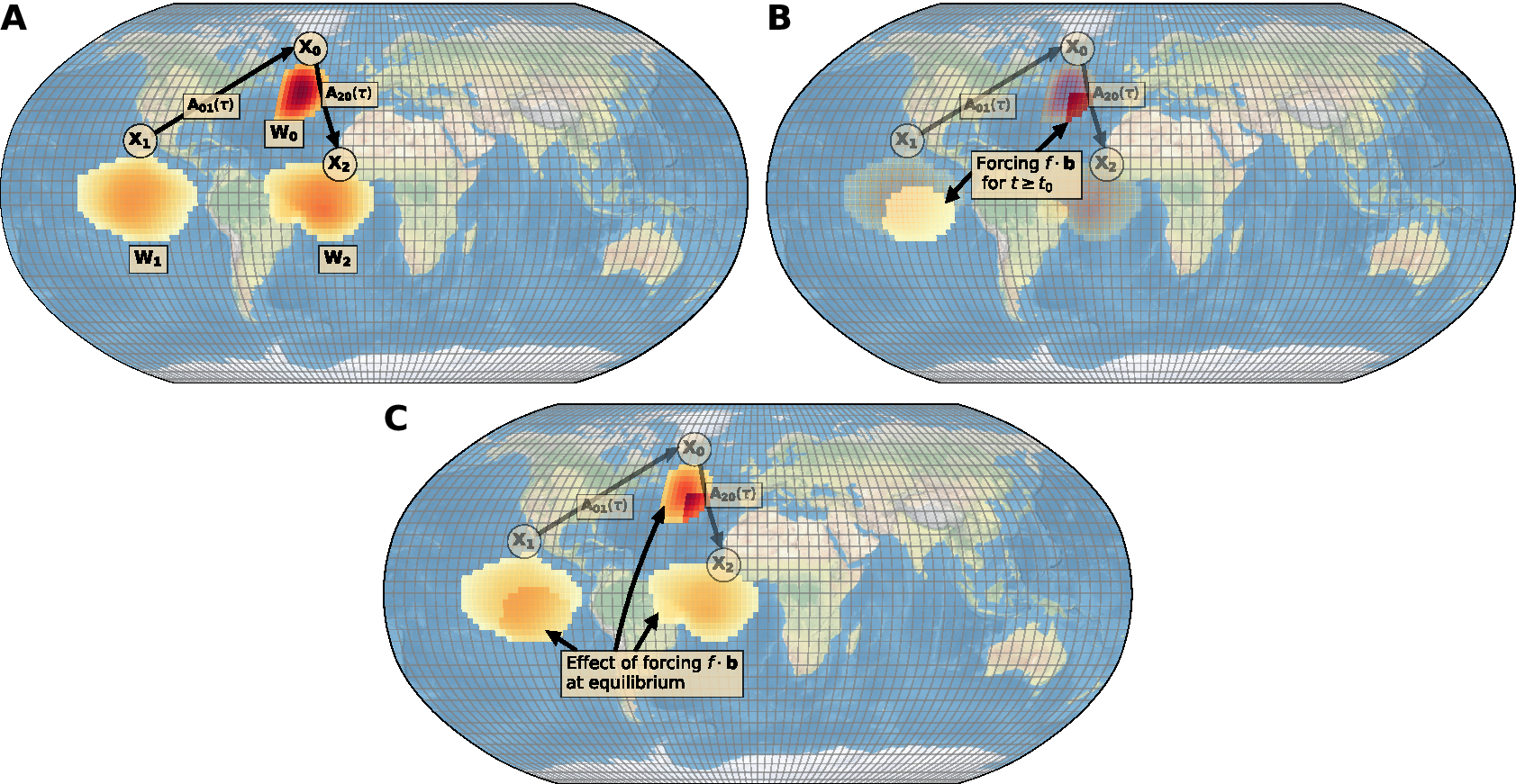
Figure 1. (A) Example of large-scale variables $ {X}_0,{X}_1,{X}_2 $
following a VAR model. Arrows indicate direct linear time dependencies between the large-scale variables defined in
$ {X}_0,{X}_1,{X}_2 $
following a VAR model. Arrows indicate direct linear time dependencies between the large-scale variables defined in $ \mathbf{A} $
, where
$ \mathbf{A} $
, where $ {\mathbf{A}}_{ij}\left(\tau \right) $
indicates the effect of variable
$ {\mathbf{A}}_{ij}\left(\tau \right) $
indicates the effect of variable $ {X}_j $
on variable
$ {X}_j $
on variable $ {X}_i $
at time lag
$ {X}_i $
at time lag $ \tau $
. The large-scale variables
$ \tau $
. The large-scale variables $ {X}_0,{X}_1,{X}_2 $
are aggregates of the small-scale variables
$ {X}_0,{X}_1,{X}_2 $
are aggregates of the small-scale variables $ \mathbf{y} $
defined on the spatial grid (gray grid) with weights
$ \mathbf{y} $
defined on the spatial grid (gray grid) with weights $ {\mathbf{W}}_{\mathbf{0}},{\mathbf{W}}_{\mathbf{1}},{\mathbf{W}}_{\mathbf{2}} $
, respectively. Each large-scale variable
$ {\mathbf{W}}_{\mathbf{0}},{\mathbf{W}}_{\mathbf{1}},{\mathbf{W}}_{\mathbf{2}} $
, respectively. Each large-scale variable $ {X}_i $
can be calculated from the small-scale variables
$ {X}_i $
can be calculated from the small-scale variables $ \mathbf{y} $
thanks to the weights vector
$ \mathbf{y} $
thanks to the weights vector $ {\mathbf{W}}_{\mathbf{i}} $
such that
$ {\mathbf{W}}_{\mathbf{i}} $
such that $ {X}_i={{\mathbf{W}}_{\mathbf{i}}}^{\prime}\mathbf{y} $
. (B) An example of an external forcing of intensity
$ {X}_i={{\mathbf{W}}_{\mathbf{i}}}^{\prime}\mathbf{y} $
. (B) An example of an external forcing of intensity $ f $
with spatial weights
$ f $
with spatial weights $ \mathbf{b} $
is applied for all time
$ \mathbf{b} $
is applied for all time $ t\ge {t}_0 $
. The forcing is constant over time, but nonuniform spatially. (C) An example of the effects of the forcing once the system reaches equilibrium (LREs). Note that the aggregation weights are obtained solely via standard dimensionality reduction methods (e.g., PCA or PCA-Varimax) or prior knowledge and are not optimized based on the linear coefficient estimation. In particular, there is no feedback from the estimation of the linear coefficients to the determination of these weights.
$ t\ge {t}_0 $
. The forcing is constant over time, but nonuniform spatially. (C) An example of the effects of the forcing once the system reaches equilibrium (LREs). Note that the aggregation weights are obtained solely via standard dimensionality reduction methods (e.g., PCA or PCA-Varimax) or prior knowledge and are not optimized based on the linear coefficient estimation. In particular, there is no feedback from the estimation of the linear coefficients to the determination of these weights.
The question we want to address is: can we quantify the effects of the forcing at the small-scale level once the processes reach equilibrium? If yes, we can calculate these effects for the small-scale variables $ \mathbf{y} $
and plot them as in Figure 1C. Answering this question is relevant as it enables the estimation of the effects of a perturbation with a higher degree of locality (at the level of the small-scale variables
$ \mathbf{y} $
and plot them as in Figure 1C. Answering this question is relevant as it enables the estimation of the effects of a perturbation with a higher degree of locality (at the level of the small-scale variables $ {y}_i $
). A standard VAR model will provide these effects only at the coarser resolution of the VAR processes (aggregated variables
$ {y}_i $
). A standard VAR model will provide these effects only at the coarser resolution of the VAR processes (aggregated variables $ {X}_i $
). There is a well-established body of literature on the estimation and the properties of the effects of a perturbation at the level of the VAR processes (Pesaran and Shin, Reference Pesaran and Shin1998; Lütkepohl, Reference Lütkepohl and Lütkepohl2005). However, to answer our motivational question, we have not found previous studies that derive similar measures at the small-scale level (
$ {X}_i $
). There is a well-established body of literature on the estimation and the properties of the effects of a perturbation at the level of the VAR processes (Pesaran and Shin, Reference Pesaran and Shin1998; Lütkepohl, Reference Lütkepohl and Lütkepohl2005). However, to answer our motivational question, we have not found previous studies that derive similar measures at the small-scale level ( $ \mathbf{y} $
) and provide their asymptotic properties and statistical significance.
$ \mathbf{y} $
) and provide their asymptotic properties and statistical significance.
To achieve this, we model the system at the small-scale level using an SAVAR model introduced in Tibau et al. (Reference Tibau, Reimers, Gerhardus, Denzler, Eyring and Runge2022). This model is an extension of a VAR model, in which the VAR processes are mapped onto small-scale variables with a matrix of weights $ \mathbf{W} $
. Going back to the example given in Figure 1, the matrix of weights of the SAVAR model could be, for example, the following:
$ \mathbf{W} $
. Going back to the example given in Figure 1, the matrix of weights of the SAVAR model could be, for example, the following:
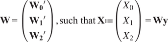 $$ \mathbf{W}=\left(\begin{array}{c}{{\mathbf{W}}_{\mathbf{0}}}^{\prime}\\ {}{{\mathbf{W}}_{\mathbf{1}}}^{\prime}\\ {}{{\mathbf{W}}_{\mathbf{2}}}^{\prime}\end{array}\right),\mathrm{such}\ \mathrm{that}\hskip0.3em \mathbf{X}:= \left(\begin{array}{c}{X}_0\\ {}{X}_1\\ {}{X}_2\end{array}\right)=\mathbf{Wy} $$
We explore the impact of a unit forcing (an external factor that influences one or several small-scale variables for all future time steps) on the global mean of system variables at equilibrium, which we refer to as sensitivity. Additionally, we investigate the effects of the forcing at the level of individual small-scale variables, providing a more detailed understanding of its impacts on the $ {y}_i $
, as opposed to the VAR processes
$ {y}_i $
, as opposed to the VAR processes $ {X}_i $
. This is characterized by the LREs, which capture the changes induced by the external forcing on the small-scale variables at equilibrium.
$ {X}_i $
. This is characterized by the LREs, which capture the changes induced by the external forcing on the small-scale variables at equilibrium.
Definition 2.2 (Sensitivity). The sensitivity quantifies the equilibrium response of global means or regional averages to a forcing, capturing the magnitude of its impact. More precisely, the sensitivity, $ \alpha $
, is defined as the ratio of the difference between the post-forcing and pre-forcing temporal averages of y over the forcing intensity f, where the temporal mean is computed over the appropriate time intervals.
$ \alpha $
, is defined as the ratio of the difference between the post-forcing and pre-forcing temporal averages of y over the forcing intensity f, where the temporal mean is computed over the appropriate time intervals.
Definition 2.3 (LREs). We define the LREs as a two-dimensional matrix, where each entry $ ij $
represents the equilibrium response of variable
$ ij $
represents the equilibrium response of variable $ {y}_i $
to a unit forcing applied to variable
$ {y}_i $
to a unit forcing applied to variable $ {y}_j $
.
$ {y}_j $
.
These two measures offer quantitative information on the effects of the forcing at the level of the small-scale variables (long-term effects) or on a specific area of interest (sensitivity) in an SAVAR model. Our approach enables the practitioner to estimate the effects of a forcing with higher locality. The effects are estimated at the finer resolution (scale of the $ {y}_i $
) rather than the coarser resolution of the VAR processes (the
$ {y}_i $
) rather than the coarser resolution of the VAR processes (the $ {X}_i $
), which will result from a standard VAR model.
$ {X}_i $
), which will result from a standard VAR model.
The previous example has motivated the need for a model that accounts for the representation of linear dependencies at the grid level. Such a representation is possible with the SAVAR model (Tibau et al., Reference Tibau, Reimers, Gerhardus, Denzler, Eyring and Runge2022). The following sections outline the SAVAR model and derive the explicit formulas for the sensitivity and LREs. We then derive the asymptotic properties of these estimators, enabling the construction of confidence intervals (CIs) for sensitivity and LREs, which can be used to quantify uncertainty and evaluate the statistical significance of the LREs at the small-scale level.
2.2. A simple spatiotemporal stochastic model: the SAVAR model
The SAVAR model introduced by Tibau et al. (Reference Tibau, Reimers, Gerhardus, Denzler, Eyring and Runge2022) is a model that combines a VAR model with a mapping. This mapping can be spatial, as described in Tibau et al. (Reference Tibau, Reimers, Gerhardus, Denzler, Eyring and Runge2022). In general, the mapping does not have to be spatial and can be any dimension that is not temporal. The mapping $ \mathbf{W}\in {\mathrm{\mathbb{R}}}^{N\times L} $
defines
$ \mathbf{W}\in {\mathrm{\mathbb{R}}}^{N\times L} $
defines $ N $
modes over
$ N $
modes over $ L $
points. The
$ L $
points. The $ N $
modes are weighted combinations of the
$ N $
modes are weighted combinations of the $ L $
grid points, thereby defining coarse-grained regions within the system. The
$ L $
grid points, thereby defining coarse-grained regions within the system. The $ N $
modes correspond to the large-scale components of the system, whereas the
$ N $
modes correspond to the large-scale components of the system, whereas the $ L $
grid points capture the small-scale features. Similar to the VAR model, the
$ L $
grid points capture the small-scale features. Similar to the VAR model, the $ N $
modes are linearly time-dependent, which we represent with the matrices of dependencies noted
$ N $
modes are linearly time-dependent, which we represent with the matrices of dependencies noted $ \mathbf{A}\left(\tau \right)\in {\mathrm{\mathbb{R}}}^{N\times N} $
. We note
$ \mathbf{A}\left(\tau \right)\in {\mathrm{\mathbb{R}}}^{N\times N} $
. We note $ {\mathbf{y}}_t\in {\mathrm{\mathbb{R}}}^L $
the vector of values of the variables on the
$ {\mathbf{y}}_t\in {\mathrm{\mathbb{R}}}^L $
the vector of values of the variables on the $ L $
points.
$ L $
points.
The SAVAR model is given in matrix notation by Tibau et al. (Reference Tibau, Reimers, Gerhardus, Denzler, Eyring and Runge2022):
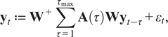 $$ {\mathbf{y}}_t\hskip0.35em := \hskip0.35em {\mathbf{W}}^{+}\sum \limits_{\tau =1}^{\tau_{\mathrm{max}}}\mathbf{A}\left(\tau \right){\mathbf{W}\mathbf{y}}_{t-\tau }+{\varepsilon}_t, $$
 $$ {\varepsilon}_t\sim \mathcal{N}\left({\mu}_{\mathbf{y}},{\boldsymbol{\Sigma}}_{\mathbf{y}}\right), $$
 $$ {\boldsymbol{\Sigma}}_{\mathbf{y}}=\lambda {\mathbf{W}}^{+}{\mathbf{D}}_{\mathbf{x}}{\mathbf{W}}^{+\mathbf{T}}+{\mathbf{D}}_{\mathbf{y}} $$
Here, we note $ {\varepsilon}_t\in {\mathrm{\mathbb{R}}}^L $
an independent noise. The noise is assumed to be independent and identically distributed. The diagonal covariance matrices
$ {\varepsilon}_t\in {\mathrm{\mathbb{R}}}^L $
an independent noise. The noise is assumed to be independent and identically distributed. The diagonal covariance matrices $ {\mathbf{D}}_{\mathbf{x}}\in {\mathrm{\mathbb{R}}}^{N\times N} $
and
$ {\mathbf{D}}_{\mathbf{x}}\in {\mathrm{\mathbb{R}}}^{N\times N} $
and $ {\mathbf{D}}_{\mathbf{y}}\in {\mathrm{\mathbb{R}}}^{L\times L} $
model the noise occurring at the mode level and the noise at each point, respectively. The covariant noise strength
$ {\mathbf{D}}_{\mathbf{y}}\in {\mathrm{\mathbb{R}}}^{L\times L} $
model the noise occurring at the mode level and the noise at each point, respectively. The covariant noise strength $ \lambda $
is a coefficient that indicates the relative strength of these two noises. We denote
$ \lambda $
is a coefficient that indicates the relative strength of these two noises. We denote $ {\mathbf{W}}^{+}\in {\mathrm{\mathbb{R}}}^{L\times N} $
the Moore–Penrose pseudoinverse of
$ {\mathbf{W}}^{+}\in {\mathrm{\mathbb{R}}}^{L\times N} $
the Moore–Penrose pseudoinverse of $ \mathbf{W} $
. As
$ \mathbf{W} $
. As $ \mathbf{W} $
is a mapping from the point level to the mode level,
$ \mathbf{W} $
is a mapping from the point level to the mode level, $ {\mathbf{W}}^{+} $
is the inverse mapping that maps from the mode level to the point level. We assume that the modes are linearly independent, such that
$ {\mathbf{W}}^{+} $
is the inverse mapping that maps from the mode level to the point level. We assume that the modes are linearly independent, such that $ \mathbf{W} $
has independent rows and is full rank. For example, a sufficient and feasible condition for linearly independent rows of
$ \mathbf{W} $
has independent rows and is full rank. For example, a sufficient and feasible condition for linearly independent rows of $ \mathbf{W} $
would be that the modes do not overlap Tibau et al. (Reference Tibau, Reimers, Gerhardus, Denzler, Eyring and Runge2022).
$ \mathbf{W} $
would be that the modes do not overlap Tibau et al. (Reference Tibau, Reimers, Gerhardus, Denzler, Eyring and Runge2022).
Although the model initially appears to include only a single process, it can be extended to accommodate as many processes as required. For example, suppose that Figure 1A shows the temperature field on $ {L}^{\prime } $
grid points and that the sea level pressure field is defined on
$ {L}^{\prime } $
grid points and that the sea level pressure field is defined on $ {L}^{{\prime\prime} } $
grid points (not shown in the figure). To include both processes, we can extend the grid to
$ {L}^{{\prime\prime} } $
grid points (not shown in the figure). To include both processes, we can extend the grid to $ L={L}^{\prime }+{L}^{{\prime\prime} } $
.
$ L={L}^{\prime }+{L}^{{\prime\prime} } $
.
The off-diagonal of $ \lambda {\mathbf{W}}^{+}{\mathbf{D}}_{\mathbf{x}}{\mathbf{W}}^{+T} $
models the covariance structure of the fast dynamics, that is, contemporaneous dependencies. The direct time-lagged dependencies at time
$ \lambda {\mathbf{W}}^{+}{\mathbf{D}}_{\mathbf{x}}{\mathbf{W}}^{+T} $
models the covariance structure of the fast dynamics, that is, contemporaneous dependencies. The direct time-lagged dependencies at time $ \tau >0 $
are modeled by
$ \tau >0 $
are modeled by $ {\mathbf{W}}^{+}\mathbf{A}\left(\tau \right)\mathbf{W} $
, which represents the emergent behavior within each mode region, leading to the collective effect rather than individual effects between single points.
$ {\mathbf{W}}^{+}\mathbf{A}\left(\tau \right)\mathbf{W} $
, which represents the emergent behavior within each mode region, leading to the collective effect rather than individual effects between single points.
Tibau et al. (Reference Tibau, Reimers, Gerhardus, Denzler, Eyring and Runge2022) also give a mode-level representation of the SAVAR model. We introduce $ {\mathbf{x}}_t\in {\mathrm{\mathbb{R}}}^N $
, such that
$ {\mathbf{x}}_t\in {\mathrm{\mathbb{R}}}^N $
, such that $ {\mathbf{x}}_t\hskip0.35em := \hskip0.35em {\mathbf{Wy}}_t $
. After left-multiplying by
$ {\mathbf{x}}_t\hskip0.35em := \hskip0.35em {\mathbf{Wy}}_t $
. After left-multiplying by $ \mathbf{W} $
in Equation (2.1) and using the property
$ \mathbf{W} $
in Equation (2.1) and using the property $ {\mathbf{WW}}^{+}={I}_N $
, where we use the notation
$ {\mathbf{WW}}^{+}={I}_N $
, where we use the notation $ {I}_n $
for the identity matrix of size
$ {I}_n $
for the identity matrix of size $ n $
, Tibau et al. (Reference Tibau, Reimers, Gerhardus, Denzler, Eyring and Runge2022) obtained the following equation for
$ n $
, Tibau et al. (Reference Tibau, Reimers, Gerhardus, Denzler, Eyring and Runge2022) obtained the following equation for $ {\mathbf{x}}_t $
:
$ {\mathbf{x}}_t $
:
 $$ {\mathbf{x}}_t=\sum \limits_{\tau =1}^{\tau_{\mathrm{max}}}\;\mathbf{A}\left(\tau \right){\mathbf{x}}_{t-\tau }+\mathbf{W}{\varepsilon}_t $$
The direct linear time-lagged dependencies between the modes are modeled with the $ \mathbf{A}\left(\tau \right) $
matrices. We assume the variability at the point level to be much smaller than the mode-level variability, which is the case for the large covariant noise strength
$ \mathbf{A}\left(\tau \right) $
matrices. We assume the variability at the point level to be much smaller than the mode-level variability, which is the case for the large covariant noise strength $ \lambda $
for which we get
$ \lambda $
for which we get $ {\boldsymbol{\Sigma}}_{\mathbf{x}}\approx \lambda {\mathbf{D}}_{\mathbf{x}} $
. Here, model-level variability refers to the variability of the aggregated mode process (
$ {\boldsymbol{\Sigma}}_{\mathbf{x}}\approx \lambda {\mathbf{D}}_{\mathbf{x}} $
. Here, model-level variability refers to the variability of the aggregated mode process ( $ {\mathbf{x}}_t $
), which is typically larger than the variability observed at the individual grid point level (
$ {\mathbf{x}}_t $
), which is typically larger than the variability observed at the individual grid point level ( $ {\mathbf{y}}_t $
).Then the model is approximately a Markovian Structural Causal Model, here a VAR model, with independent noise terms (Tibau et al., Reference Tibau, Reimers, Gerhardus, Denzler, Eyring and Runge2022). The statistical properties of the SAVAR process, such as stationarity, stability, and identifiability, are deduced in Tibau et al. (Reference Tibau, Reimers, Gerhardus, Denzler, Eyring and Runge2022). Under the assumptions detailed in Tibau et al. (Reference Tibau, Reimers, Gerhardus, Denzler, Eyring and Runge2022), the stationarity and stability of the SAVAR process are guaranteed by the corresponding properties of the underlying mode-space VAR process. Similarly to VAR models, SAVAR models can be augmented with an exogenous term, which is particularly useful for incorporating specific characteristics of the data into the analysis. For instance, seasonal dummy variables can be added to an SAVAR model to account for periodic patterns in the data.
$ {\mathbf{y}}_t $
).Then the model is approximately a Markovian Structural Causal Model, here a VAR model, with independent noise terms (Tibau et al., Reference Tibau, Reimers, Gerhardus, Denzler, Eyring and Runge2022). The statistical properties of the SAVAR process, such as stationarity, stability, and identifiability, are deduced in Tibau et al. (Reference Tibau, Reimers, Gerhardus, Denzler, Eyring and Runge2022). Under the assumptions detailed in Tibau et al. (Reference Tibau, Reimers, Gerhardus, Denzler, Eyring and Runge2022), the stationarity and stability of the SAVAR process are guaranteed by the corresponding properties of the underlying mode-space VAR process. Similarly to VAR models, SAVAR models can be augmented with an exogenous term, which is particularly useful for incorporating specific characteristics of the data into the analysis. For instance, seasonal dummy variables can be added to an SAVAR model to account for periodic patterns in the data.
2.3. Derivation of the LREs and sensitivity in an SAVAR model
In the considered framework, the introduction and the motivating example of Section 2.1 have displayed the importance of measures that identify the effects of a perturbation in a system at the small-scale level. We introduce such measures and derive their explicit formulas in an SAVAR model.
2.3.1. Sensitivity in an SAVAR model
We call a forcing of intensity $ f $
and of weights
$ f $
and of weights $ \mathbf{b}\in {\mathrm{\mathbb{R}}}^L $
an external perturbation that is applied to the system, as illustrated in Figure 1B. We assume that the underlying VAR process is stable before the application of the forcing, which is then introduced after the system has reached equilibrium. Without loss of generality, we assume that the forcing is applied at time
$ \mathbf{b}\in {\mathrm{\mathbb{R}}}^L $
an external perturbation that is applied to the system, as illustrated in Figure 1B. We assume that the underlying VAR process is stable before the application of the forcing, which is then introduced after the system has reached equilibrium. Without loss of generality, we assume that the forcing is applied at time $ {t}_0 $
and that there was no forcing for
$ {t}_0 $
and that there was no forcing for $ t<{t}_0 $
. For
$ t<{t}_0 $
. For $ t\ge {t}_0 $
, the forcing is constant but does not have to be uniform. Each coefficient
$ t\ge {t}_0 $
, the forcing is constant but does not have to be uniform. Each coefficient $ {\mathbf{b}}_i $
of
$ {\mathbf{b}}_i $
of $ \mathbf{b} $
represents the weighting of the forcing at grid point
$ \mathbf{b} $
represents the weighting of the forcing at grid point $ i $
. In this context, the sensitivity is a measure that indicates the average effect of the forcing on the system (or a custom region of interest) at equilibrium (the system reaches a stable state) normalized by the value of its intensity
$ i $
. In this context, the sensitivity is a measure that indicates the average effect of the forcing on the system (or a custom region of interest) at equilibrium (the system reaches a stable state) normalized by the value of its intensity $ f $
. For
$ f $
. For $ t\ge {t}_0 $
, we have:
$ t\ge {t}_0 $
, we have:
 $$ {\mathbf{y}}_t\hskip0.35em := \hskip0.35em {\mathbf{W}}^{+}\sum \limits_{\tau =1}^{\tau_{\mathrm{max}}}\mathbf{A}\left(\tau \right){\mathbf{W}\mathbf{y}}_{t-\tau }+f\mathbf{b}+{\varepsilon}_t $$
The forcing weights vector $ \mathbf{b} $
is assumed to be known a priori and specifies the spatial pattern of the external perturbation. The definition of the sensitivity, denoted by
$ \mathbf{b} $
is assumed to be known a priori and specifies the spatial pattern of the external perturbation. The definition of the sensitivity, denoted by $ \alpha $
, is given by the following formula:
$ \alpha $
, is given by the following formula:
 $$ \alpha \hskip0.35em := \hskip0.35em \frac{\overline{\left\langle {\mathbf{y}}_{t>{t}_0}\right\rangle }-\overline{\left\langle {\mathbf{y}}_{t<{t}_0}\right\rangle }}{f} $$
where $ \left\langle \mathbf{y}\right\rangle $
denotes the temporal mean of
$ \left\langle \mathbf{y}\right\rangle $
denotes the temporal mean of $ \mathbf{y} $
. Here,
$ \mathbf{y} $
. Here, $ \overline{\mathbf{y}} $
is the mean of
$ \overline{\mathbf{y}} $
is the mean of $ \mathbf{y} $
over all the
$ \mathbf{y} $
over all the $ L $
points or over a specific area of interest such that
$ L $
points or over a specific area of interest such that $ \overline{\mathbf{y}}=\frac{1}{\parallel \mathbf{h}{\parallel}_1}{\mathbf{h}}^{\prime}\mathbf{y} $
. Here,
$ \overline{\mathbf{y}}=\frac{1}{\parallel \mathbf{h}{\parallel}_1}{\mathbf{h}}^{\prime}\mathbf{y} $
. Here, $ \mathbf{h} $
denotes a column vector with ones for the points inside the custom region of interest and zeros otherwise.
$ \mathbf{h} $
denotes a column vector with ones for the points inside the custom region of interest and zeros otherwise.
In the following, we assume that $ {\mathbf{x}}_t $
is a stable VAR process as defined in Equation (2.2). Then,
$ {\mathbf{x}}_t $
is a stable VAR process as defined in Equation (2.2). Then, $ {\mathbf{y}}_t $
as defined in Equation (2.1) is also a stable SAVAR process (see proof in Tibau et al., Reference Tibau, Reimers, Gerhardus, Denzler, Eyring and Runge2022). Using the formula of the SAVAR model
$ {\mathbf{y}}_t $
as defined in Equation (2.1) is also a stable SAVAR process (see proof in Tibau et al., Reference Tibau, Reimers, Gerhardus, Denzler, Eyring and Runge2022). Using the formula of the SAVAR model $ {\mathbf{y}}_t $
, one can derive two explicit formulas of
$ {\mathbf{y}}_t $
, one can derive two explicit formulas of $ \alpha $
:
$ \alpha $
:
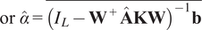
 $$ \alpha =\overline{{\left({I}_L-{\mathbf{W}}^{+}\mathbf{AKW}\right)}^{-1}\mathbf{b}} $$
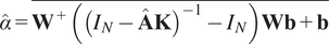
 $$ \mathrm{and}\hskip0.4em \alpha =\overline{{\mathbf{W}}^{+}\left({\left({I}_N-\mathbf{AK}\right)}^{-1}-{I}_N\right)\mathbf{Wb}+\mathbf{b}} $$
where we introduce the block matrices: $ \mathbf{A}=\left(\mathbf{A}(1),\hskip0.5em \mathbf{A}(2),\hskip0.5em \dots, \hskip0.5em \mathbf{A}\left({\tau}_{\mathrm{max}}\right)\right) $
and
$ \mathbf{A}=\left(\mathbf{A}(1),\hskip0.5em \mathbf{A}(2),\hskip0.5em \dots, \hskip0.5em \mathbf{A}\left({\tau}_{\mathrm{max}}\right)\right) $
and $ {\mathbf{K}}^{\prime }=\left(\begin{array}{cccc}{I}_N,& {I}_N,& \dots, & {I}_N\end{array}\right) $
such that the product
$ {\mathbf{K}}^{\prime }=\left(\begin{array}{cccc}{I}_N,& {I}_N,& \dots, & {I}_N\end{array}\right) $
such that the product $ \mathbf{AK}={\sum}_{\tau =1}^{\tau_{\mathrm{max}}}\mathbf{A}\left(\tau \right) $
to facilitate future derivations. We recall that
$ \mathbf{AK}={\sum}_{\tau =1}^{\tau_{\mathrm{max}}}\mathbf{A}\left(\tau \right) $
to facilitate future derivations. We recall that $ N $
denotes the number of modes and
$ N $
denotes the number of modes and $ L $
is the number of points. Equations (2.3b) and (2.3c) provide two mathematically equivalent formulations for the sensitivity
$ L $
is the number of points. Equations (2.3b) and (2.3c) provide two mathematically equivalent formulations for the sensitivity $ \alpha $
as derived from the SAVAR model. The calculations leading to the two explicit formulas are detailed in Appendix A.1.
$ \alpha $
as derived from the SAVAR model. The calculations leading to the two explicit formulas are detailed in Appendix A.1.
We notice that the value of the forcing $ f $
does not appear in the explicit formula. However, the forcing weights
$ f $
does not appear in the explicit formula. However, the forcing weights $ \mathbf{b} $
play a role in the calculation of the sensitivity. We also point out that the sensitivity depends on the mode weights
$ \mathbf{b} $
play a role in the calculation of the sensitivity. We also point out that the sensitivity depends on the mode weights $ \mathbf{W} $
and on the matrices of linear time-lagged dependencies
$ \mathbf{W} $
and on the matrices of linear time-lagged dependencies $ \mathbf{A}\left(\tau \right) $
.
$ \mathbf{A}\left(\tau \right) $
.
2.3.2. LREs in an SAVAR model
The explicit formula for sensitivity shows the role of the forcing weights $ \mathbf{b} $
. If the forcing
$ \mathbf{b} $
. If the forcing $ f $
involves only a single grid point, for example, grid point
$ f $
involves only a single grid point, for example, grid point $ i $
with weight
$ i $
with weight $ 1 $
,
$ 1 $
, $ \mathbf{b} $
is then a vector of zeros except for
$ \mathbf{b} $
is then a vector of zeros except for $ {b}_i=1 $
. By introducing the matrix
$ {b}_i=1 $
. By introducing the matrix $ {\boldsymbol{\Psi}}_{\infty } $
such that
$ {\boldsymbol{\Psi}}_{\infty } $
such that $ \alpha \hskip0.35em := \hskip0.35em \overline{{\boldsymbol{\Psi}}_{\infty}\mathbf{b}} $
, we notice that only the coefficient of the
$ \alpha \hskip0.35em := \hskip0.35em \overline{{\boldsymbol{\Psi}}_{\infty}\mathbf{b}} $
, we notice that only the coefficient of the $ i $
th column of
$ i $
th column of $ {\boldsymbol{\Psi}}_{\infty } $
play a role in the calculation of the sensitivity. The coefficient
$ {\boldsymbol{\Psi}}_{\infty } $
play a role in the calculation of the sensitivity. The coefficient $ {\left({\boldsymbol{\Psi}}_{\infty}\right)}_{ij} $
indicates the effect of a unit forcing at grid point
$ {\left({\boldsymbol{\Psi}}_{\infty}\right)}_{ij} $
indicates the effect of a unit forcing at grid point $ j $
on grid
$ j $
on grid $ i $
at equilibrium. For this reason, we refer to
$ i $
at equilibrium. For this reason, we refer to $ {\boldsymbol{\Psi}}_{\infty } $
as the matrix of LREs. For an SAVAR model, the LREs are given by explicit formulas:
$ {\boldsymbol{\Psi}}_{\infty } $
as the matrix of LREs. For an SAVAR model, the LREs are given by explicit formulas:
 $$ {\boldsymbol{\Psi}}_{\infty }={\mathbf{W}}^{+}\left({\left({I}_N-\mathbf{AK}\right)}^{-1}-{I}_N\right)\mathbf{W}+{I}_L $$
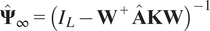
 $$ {\boldsymbol{\Psi}}_{\infty }={\left({I}_L-{\mathbf{W}}^{+}\mathbf{AKW}\right)}^{-1} $$
Both Expressions (2.4a) and (2.4b) provide equivalent representation under the model assumptions. The coefficient of the LREs $ {\left({\boldsymbol{\Psi}}_{\infty}\right)}_{ij} $
indicates the long-term effect of a unit change in grid point
$ {\left({\boldsymbol{\Psi}}_{\infty}\right)}_{ij} $
indicates the long-term effect of a unit change in grid point $ j $
on grid point
$ j $
on grid point $ i $
. We can also interpret
$ i $
. We can also interpret $ {\boldsymbol{\Psi}}_{\infty } $
in terms of columns. The
$ {\boldsymbol{\Psi}}_{\infty } $
in terms of columns. The $ j $
th column of
$ j $
th column of $ {\boldsymbol{\Psi}}_{\infty } $
contains the long-term effects of a unit change in the
$ {\boldsymbol{\Psi}}_{\infty } $
contains the long-term effects of a unit change in the $ j $
th small-scale variable of the system. In a standard VAR model, the LREs matrix can be derived for a shock (Lütkepohl, Reference Lütkepohl and Lütkepohl2005) and has a similar form:
$ j $
th small-scale variable of the system. In a standard VAR model, the LREs matrix can be derived for a shock (Lütkepohl, Reference Lütkepohl and Lütkepohl2005) and has a similar form: $ {\boldsymbol{\Psi}}_{\infty }={\left({I}_N-\mathbf{AK}\right)}^{-1} $
. Unlike Equations (2.4a) and (2.4b), this latter formula does not include the matrix of weights
$ {\boldsymbol{\Psi}}_{\infty }={\left({I}_N-\mathbf{AK}\right)}^{-1} $
. Unlike Equations (2.4a) and (2.4b), this latter formula does not include the matrix of weights $ \mathbf{W} $
, which expresses the aggregation of the large-scale variables in the SAVAR model.
$ \mathbf{W} $
, which expresses the aggregation of the large-scale variables in the SAVAR model.
2.3.3. Estimation
If $ \mathbf{W} $
is known, and
$ \mathbf{W} $
is known, and $ \mathbf{A} $
is estimated, one can also estimate
$ \mathbf{A} $
is estimated, one can also estimate $ \alpha $
and
$ \alpha $
and $ {\boldsymbol{\Psi}}_{\infty } $
by plugging them in the explicit formulas of
$ {\boldsymbol{\Psi}}_{\infty } $
by plugging them in the explicit formulas of $ \alpha $
and
$ \alpha $
and $ {\boldsymbol{\Psi}}_{\infty } $
.
$ {\boldsymbol{\Psi}}_{\infty } $
.
Given an estimator $ \hat{\mathbf{A}} $
of
$ \hat{\mathbf{A}} $
of $ \mathbf{A} $
,
$ \mathbf{A} $
, $ \hat{\alpha} $
introduced below is an estimator of
$ \hat{\alpha} $
introduced below is an estimator of $ \alpha $
:
$ \alpha $
:
 $$ \hat{\alpha}=\overline{{\mathbf{W}}^{+}\left({\left({I}_N-\hat{\mathbf{A}}\mathbf{K}\right)}^{-1}-{I}_N\right)\mathbf{Wb}+\mathbf{b}} $$
 $$ \mathrm{or}\hskip0.4em \hat{\alpha}=\overline{{\left({I}_L-{\mathbf{W}}^{+}\hat{\mathbf{A}}\mathbf{KW}\right)}^{-1}\mathbf{b}} $$
And an estimator $ {\hat{\boldsymbol{\Psi}}}_{\infty } $
of
$ {\hat{\boldsymbol{\Psi}}}_{\infty } $
of $ {\boldsymbol{\Psi}}_{\infty } $
is given by:
$ {\boldsymbol{\Psi}}_{\infty } $
is given by:
 $$ {\hat{\boldsymbol{\Psi}}}_{\infty }={\left({I}_L-{\mathbf{W}}^{+}\hat{\mathbf{A}}\mathbf{KW}\right)}^{-1} $$
2.4. Asymptotic distribution of the LREs and sensitivity estimators
We then derive the asymptotic distributions of the estimated sensitivity and LREs. If $ \mathbf{W} $
is known and
$ \mathbf{W} $
is known and $ \mathbf{A} $
is estimated, then in Proposition 2.1, we give the asymptotic distributions for
$ \mathbf{A} $
is estimated, then in Proposition 2.1, we give the asymptotic distributions for $ {\hat{\boldsymbol{\Psi}}}_{\infty } $
and
$ {\hat{\boldsymbol{\Psi}}}_{\infty } $
and $ \hat{\alpha} $
under the assumptions.
$ \hat{\alpha} $
under the assumptions.
Proposition 2.1. (Asymptotic distribution of $ \hat{\alpha} $
and
$ \hat{\alpha} $
and $ {\hat{\Psi}}_{\infty } $
).
$ {\hat{\Psi}}_{\infty } $
).
Let $ {\mathbf{x}}_t $
be a stable VAR process as defined in Equation (2.2). Then,
$ {\mathbf{x}}_t $
be a stable VAR process as defined in Equation (2.2). Then, $ {\mathbf{y}}_t $
as defined in Equation (2.1) is also a stable SAVAR process (see proof in Tibau et al., Reference Tibau, Reimers, Gerhardus, Denzler, Eyring and Runge2022). This implies that
$ {\mathbf{y}}_t $
as defined in Equation (2.1) is also a stable SAVAR process (see proof in Tibau et al., Reference Tibau, Reimers, Gerhardus, Denzler, Eyring and Runge2022). This implies that $ {\left({I}_L-{\mathbf{W}}^{+}\mathbf{AKW}\right)}^{-1} $
and
$ {\left({I}_L-{\mathbf{W}}^{+}\mathbf{AKW}\right)}^{-1} $
and $ {\left({I}_N-\mathbf{AK}\right)}^{-1} $
are invertible. We note
$ {\left({I}_N-\mathbf{AK}\right)}^{-1} $
are invertible. We note $ \hat{\beta}= vec\left(\hat{\mathbf{A}}\right) $
and
$ \hat{\beta}= vec\left(\hat{\mathbf{A}}\right) $
and $ \beta = vec\left(\mathbf{A}\right) $
where
$ \beta = vec\left(\mathbf{A}\right) $
where $ vec $
denotes the vectorization of a matrix (see Appendix A.2).
$ vec $
denotes the vectorization of a matrix (see Appendix A.2). $ T $
is the sample size.
$ T $
is the sample size.
If
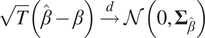 $$ \sqrt{T}\left(\hat{\beta}-\beta \right)\overset{d}{\to}\mathcal{N}\left(0,{\boldsymbol{\Sigma}}_{\hat{\beta}}\right) $$
Then,
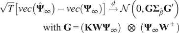 $$ {\displaystyle \begin{array}{r}\sqrt{T}\left[ vec\left({\hat{\boldsymbol{\Psi}}}_{\infty}\right)- vec\left({\boldsymbol{\Psi}}_{\infty}\right)\right]\overset{d}{\to}\mathcal{N}\left(0,\mathbf{G}{\boldsymbol{\Sigma}}_{\hat{\beta}}{\mathbf{G}}^{\prime}\right)\\ {}\mathrm{with}\hskip0.4em \mathbf{G}={\left(\mathbf{KW}{\boldsymbol{\Psi}}_{\infty}\right)}^{\hskip0.5em }\hskip0.4em \otimes \hskip0.7em \left({\boldsymbol{\Psi}}_{\infty }{\mathbf{W}}^{+}\right)\end{array}} $$
And
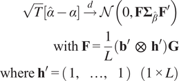 $$ {\displaystyle \begin{array}{r}\sqrt{T}\left[\hat{\alpha}-\alpha \right]\overset{d}{\to}\mathcal{N}\left(0,\mathbf{F}{\boldsymbol{\Sigma}}_{\hat{\beta}}{\mathbf{F}}^{\prime}\right)\\ {}\mathrm{with}\hskip0.32em \mathbf{F}=\frac{1}{L}\left({\mathbf{b}}^{\prime}\hskip0.5em \otimes \hskip0.5em {\mathbf{h}}^{\prime}\right)\mathbf{G}\\ {}\mathrm{where}\hskip0.32em {\mathbf{h}}^{\prime }=\left(\begin{array}{ccc}1,& \dots, & 1\end{array}\right)\hskip1em \left(1\times L\right)\end{array}} $$
The normal distribution is represented by the symbol $ \mathcal{N} $
, and the Kronecker product is denoted by the symbol
$ \mathcal{N} $
, and the Kronecker product is denoted by the symbol $ \otimes $
. The proofs can be found in Appendix A.3.
$ \otimes $
. The proofs can be found in Appendix A.3.
2.4.1. Assumptions and estimation
Here are some important comments regarding this last proposition:
-
• Assumptions: One key assumption is that the distribution of the estimated matrix of linear coefficients is asymptotically normally distributed and that the estimator of the linear coefficient is consistent, which is the case, for instance, when $ \mathbf{W} $
is known and
$ \mathbf{A} $
is estimated using the least-squares estimator (Lütkepohl, Reference Lütkepohl and Lütkepohl2005).
$ \mathbf{W} $
is known and
$ \mathbf{A} $
is estimated using the least-squares estimator (Lütkepohl, Reference Lütkepohl and Lütkepohl2005). -
• Implications: The proposition demonstrates that the estimators of the LREs and sensitivity are consistent. In addition, the proposition gives the asymptotic distribution of the estimators, which are normal distributions.
-
• When the sensitivity is not computed on all the
$ L $
points, one has to replace
$ \mathbf{h} $
by a vector with one coefficient for the
$ \tilde{L}\le L $
small-scale variables of interest and a zero coefficient elsewhere. Then, in the expression of
$ F $
,
$ \frac{1}{L} $
has to be replaced by
$ \frac{1}{\tilde{L}} $
. -
• To estimate the covariance matrix of the linear coefficients
$ {\boldsymbol{\Sigma}}_{\hat{\beta}} $
in practice, we use the consistent estimator provided in Lütkepohl (Reference Lütkepohl and Lütkepohl2005) for a VAR model:
$ {\hat{\boldsymbol{\Sigma}}}_{\hat{\beta}}=\frac{\mathbf{Z}{\mathbf{Z}}^{\prime }}{T}\hskip0.5em \otimes \hskip0.5em {\hat{\boldsymbol{\Sigma}}}_{\varepsilon } $
. We define
$ \mathbf{Z}\hskip0.35em := \hskip0.35em \left({\mathbf{Z}}_0,\dots, {\mathbf{Z}}_{T-1}\right) $
where
$ {\mathbf{Z}}_t^{\prime }=\left[\begin{array}{cccc}1& {\mathbf{y}}_t^{\prime }& \cdots & {\mathbf{y}}_{t-{\tau}_{\mathrm{max}}+1}^{\prime}\end{array}\right] $
. And
$ {\hat{\boldsymbol{\Sigma}}}_{\varepsilon } $
is an unbiased estimator of the covariance matrix of the residuals.
$ {\hat{\boldsymbol{\Sigma}}}_{\varepsilon }=\frac{\hat{\varepsilon}{\hat{\varepsilon}}^{\prime }}{T-P} $
, here
$ \hat{\varepsilon} $
are the estimated residuals and
$ P $
is the total number of parameters of the VAR model embedded in the SAVAR model.


2.4.2. CI and statistical significance
If the actual asymptotic distributions of the LREs and sensitivity are not degenerate, we can derive asymptotic CIs from the asymptotic variance of the sensitivity and covariance matrix of the LREs (Benkwitz et al., Reference Benkwitz, Lutkepohl and Neumann1997; Lütkepohl, Reference Lütkepohl and Lütkepohl2005). For example, to obtain the $ \omega $
% CI of a specific LRE
$ \omega $
% CI of a specific LRE $ {\left({\boldsymbol{\Psi}}_{\infty}\right)}_{ij} $
, we first retrieve the associated diagonal element of the covariance matrix of the LREs. This gives us
$ {\left({\boldsymbol{\Psi}}_{\infty}\right)}_{ij} $
, we first retrieve the associated diagonal element of the covariance matrix of the LREs. This gives us $ {\hat{\sigma}}_{{\left({\boldsymbol{\Psi}}_{\infty}\right)}_{ij}}^2 $
, an estimate of the asymptotic variance of the LREs
$ {\hat{\sigma}}_{{\left({\boldsymbol{\Psi}}_{\infty}\right)}_{ij}}^2 $
, an estimate of the asymptotic variance of the LREs $ {\left({\boldsymbol{\Psi}}_{\infty}\right)}_{ij} $
. Then, the asymptotic CI is given by the interval between the
$ {\left({\boldsymbol{\Psi}}_{\infty}\right)}_{ij} $
. Then, the asymptotic CI is given by the interval between the $ \frac{\omega }{2} $
quantile and
$ \frac{\omega }{2} $
quantile and $ 1-\frac{\omega }{2} $
quantile of a normal distribution with mean
$ 1-\frac{\omega }{2} $
quantile of a normal distribution with mean $ {\left({\hat{\boldsymbol{\Psi}}}_{\infty}\right)}_{ij} $
and variance
$ {\left({\hat{\boldsymbol{\Psi}}}_{\infty}\right)}_{ij} $
and variance $ {\hat{\sigma}}_{{\left({\boldsymbol{\Psi}}_{\infty}\right)}_{ij}}^2 $
. Furthermore, the estimated LRE
$ {\hat{\sigma}}_{{\left({\boldsymbol{\Psi}}_{\infty}\right)}_{ij}}^2 $
. Furthermore, the estimated LRE $ {\left({\hat{\boldsymbol{\Psi}}}_{\infty}\right)}_{ij} $
is significantly different from zero at an asymptotic
$ {\left({\hat{\boldsymbol{\Psi}}}_{\infty}\right)}_{ij} $
is significantly different from zero at an asymptotic $ \frac{\omega }{2} $
level if the latter CI does not contain the value zero. The proposed asymptotic-based CIs can be used to assess significance at the level of the small-scale variables, allowing for a more localized assessment of the effects of a perturbation.
$ \frac{\omega }{2} $
level if the latter CI does not contain the value zero. The proposed asymptotic-based CIs can be used to assess significance at the level of the small-scale variables, allowing for a more localized assessment of the effects of a perturbation.
3. Numerical results
We have introduced materials and methods to estimate the sensitivity and LREs in an SAVAR model. In the next section, we numerically estimate these measures from synthetic data and real-world data while providing uncertainty ranges.
3.1. Synthetic data experiments
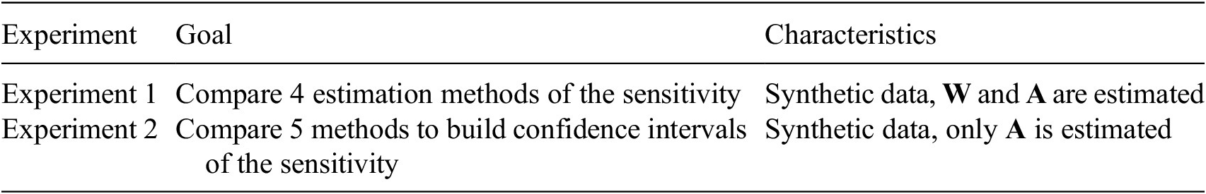
We designed two experiments with synthetic data summarized in Table 1. In Experiment 1, we carried out a benchmark analysis of four methods to estimate the sensitivity for varying SAVAR parameters. The synthetic data are generated from an SAVAR model. The sensitivity values are calculated from the explicit formulas with the estimated weights and linear coefficients. We included two methods to estimate the weights and two methods to estimate the linear coefficients. This gave us four combinations of methods to estimate the sensitivity. In Experiment 2, we compared five methods to obtain an uncertainty estimation of the sensitivity with CIs. In Experiment 1, both the aggregation weights W and the linear coefficient matrix A are estimated to assess the full estimation pipeline, whereas in Experiment 2, we assume that $ W $
is known in order to isolate the effect of
$ W $
is known in order to isolate the effect of $ A $
estimation on the uncertainty quantification.
$ A $
estimation on the uncertainty quantification.
Table 1. Summary of the synthetic data experiments
3.1.1. Methods to estimate the sensitivity and LREs
The goal of Experiment 1 is to evaluate which estimation methods are best for estimating sensitivity and LREs from data. For this, we compared four methods to estimate sensitivity from SAVAR-generated data in the case where the weight matrix $ \mathbf{W} $
is unknown. Each method consists of two distinct steps: the weight matrix estimation and the linear coefficients estimation. We estimated and evaluated the sensitivity from these estimated weights and linear coefficient matrices. In the main body of this article, we chose to evaluate the sensitivity, as the evaluation of this one-dimensional measure is more interpretable. We conducted separate benchmarks for the LREs, and the results are presented in the Appendix. We included the following methods in the benchmark analysis:
$ \mathbf{W} $
is unknown. Each method consists of two distinct steps: the weight matrix estimation and the linear coefficients estimation. We estimated and evaluated the sensitivity from these estimated weights and linear coefficient matrices. In the main body of this article, we chose to evaluate the sensitivity, as the evaluation of this one-dimensional measure is more interpretable. We conducted separate benchmarks for the LREs, and the results are presented in the Appendix. We included the following methods in the benchmark analysis:
-
• PCA followed by a VAR estimation
-
• PCA followed by Peter and Clark Momentary Conditional Independence (PCMCI) and a Causal Coefficient Matrix (CCM) estimation
-
• PCA-Varimax followed by a VAR estimation
-
• PCA-Varimax followed by PCMCI and a CCM estimation
To estimate the weights, two methods are compared: the PCA and the PCA-Varimax. PCA is a dimension-reduction technique that aims to maximize the variance of the components (Shaffer, Reference Shaffer2002). Additionally, PCA components must satisfy a constraint of orthogonality. Varimax is another dimension-reduction technique that builds on PCA. In the Varimax method, the PCA components are first calculated, and then these components are Varimax-rotated. The Varimax rotation follows a specific criterion (Kaiser, Reference Kaiser1958; Vautard and Ghil, Reference Vautard and Ghil1989), which makes the large PCA loadings larger and the small loadings smaller. This rotation allows the original PCA components to become non-orthogonal and more regionally confined, thereby generally enhancing the interpretability of the components (Rohe and Zeng, Reference Rohe and Zeng2023).
Next, we included two methods to estimate the linear coefficients of an SAVAR model. First, a simple least-squares VAR estimation, which we refer to as VAR estimation, is performed on the estimated components’ time series. We use the VAR estimation (Johansen, Reference Johansen and Johansen1995; Lütkepohl, Reference Lütkepohl and Lütkepohl2005), implemented in the statsmodel Python package (Seabold and Perktold, Reference Seabold and Perktold2010). The second method we include, referred to as PCMCI–CCM, exploits causality to constrain the linear coefficients to only causal dependencies in a two-step procedure. In the first step, we use a time series causal discovery algorithm, here PCMCI (Runge et al., Reference Runge, Petoukhov, Donges, Hlinka, Jajcay, Vejmelka, Hartman, Marwan, Paluš and Kurths2015; Runge et al., Reference Runge, Nowack, Kretschmer, Flaxman and Sejdinovic2019), to estimate the causal parents of each mode from the time series data. By causal parent, we refer to a direct cause of the specific variable in question. PCMCI is fundamentally different from PCA, which is used only for dimensionality reduction. PCMCI uses conditional independence tests to infer causal relationships between variables. In the second step, called CCM estimation, we estimate the linear coefficients solely for the causal dependencies identified in the previous step. PCMCI is a causal discovery algorithm adapted for time series, which estimates the time-lagged dependencies from input time series data. The PCMCI is available in the tigramite Python package at https://github.com/jakobrunge/tigramite. The CCM is estimated by performing a linear regression with ordinary least squares on the estimated causal parents. Note that the use of PCMCI comes with certain assumptions such as causal sufficiency, acyclicity, causal stationarity, causal faithfulness, and the causal Markov condition (Spirtes et al., Reference Spirtes, Glymour and Scheines1993; Runge et al., Reference Runge, Gerhardus, Varando, Eyring and Camps-Valls2023). Causal sufficiency requires the absence of unobserved variables. Causal stationarity assumes that the causal relationships and noise distributions are invariant in time. The causal faithfulness assumption and the causal Markov condition are necessary to establish the equivalence between the connectivity of causal graphs (precisely, d-separation) and conditional independence in the distribution (Runge et al., Reference Runge, Gerhardus, Varando, Eyring and Camps-Valls2023). PCMCI utilizes this property to perform statistical tests of independence from observational data. These tests provide insights that refine the structure of causal graphs. To test the conditional independence, we employ the linear partial correlation test of PCMCI. Throughout all numerical experiments, including both synthetic and real-world data, the PCMCI parameter $ {\alpha}_{PC} $
is internally optimized. The reader can refer to (Runge et al., Reference Runge, Nowack, Kretschmer, Flaxman and Sejdinovic2019) for an in-depth explanation of PCMCI.
$ {\alpha}_{PC} $
is internally optimized. The reader can refer to (Runge et al., Reference Runge, Nowack, Kretschmer, Flaxman and Sejdinovic2019) for an in-depth explanation of PCMCI.
3.1.2. Methods to quantify uncertainties of the estimates (CIs)
In Experiment 2, we explored various methods for establishing CIs around sensitivity estimates. Several techniques exist for deriving CIs. In our study, we examined four bootstrap methods, which involved resampling residuals similar to techniques used in impulse response analysis (Benkwitz et al., Reference Benkwitz, Lütkepohl and Wolters2001; Lütkepohl, Reference Lütkepohl and Lütkepohl2005), along with the asymptotic-based CI outlined in Section 2.4.2. This resulted in a total of five distinct methods, listed below:
-
• Bootstrapping with resampling of the residuals (Efron and Tibshirani, Reference Efron and Tibshirani1995) and standard percentile interval (abbreviated to Res-Standard),
-
• Bootstrapping with resampling of the residuals and with Hall’s percentile interval (Hall, Reference Hall1992) (abbreviated to Res-Hall),
-
• Bootstrapping with sampling from the covariance of the residuals (Efron and Tibshirani, Reference Efron and Tibshirani1995) and standard percentile interval (abbreviated to Cov-Standard),
-
• Bootstrapping with sampling from the covariance of the residuals and with Hall’s percentile interval (Hall, Reference Hall1992) (abbreviated to Cov-Hall),
-
• CI based on the asymptotic normal distribution of the estimator we have derived in Section 2.4.2 (abbreviated to Asymp.).
Throughout the rest of this article, we refer to confidence interval as CI. For further information on the various bootstrap procedures, please refer to Appendix A.4. In this experiment, we assumed that the true weights, denoted as $ \mathbf{W} $
, are known. However, only the linear coefficients, represented by
$ \mathbf{W} $
, are known. However, only the linear coefficients, represented by $ \mathbf{A} $
, are estimated. This estimation is performed using either the PCMCI–CCM method or the VAR estimation.
$ \mathbf{A} $
, are estimated. This estimation is performed using either the PCMCI–CCM method or the VAR estimation.
3.1.3. Setup of Experiment 1
In Experiment 1, we performed a benchmark analysis of the methods introduced in Section 3.1.1 to estimate the sensitivity from synthetic data. In particular, we considered the global sensitivity (i.e., the global effects over all small-scale variables) for a uniform and constant unit forcing.
Similar to the numerical experiments in Tibau et al. (Reference Tibau, Reimers, Gerhardus, Denzler, Eyring and Runge2022), the synthetic data are generated from an SAVAR model (see Equation (2.1)). The weights of the $ N $
modes
$ N $
modes $ \mathbf{W} $
are generated randomly from nonoverlapping boxes in a space of size
$ \mathbf{W} $
are generated randomly from nonoverlapping boxes in a space of size $ 20\times 30 $
(called resolution). Their shape is that of a bivariate Gaussian distribution computed from a random positive-definite covariance matrix. The underlying causal dependencies among these modes are modeled by the matrix
$ 20\times 30 $
(called resolution). Their shape is that of a bivariate Gaussian distribution computed from a random positive-definite covariance matrix. The underlying causal dependencies among these modes are modeled by the matrix $ \mathbf{A} $
given in Equation (2.1). All modes are autocorrelated and have coefficients drawn from a truncated Gaussian distribution with a mean of 0.3 (called auto-coefficient strength) and a variance of 0.2. The coefficients have an absolute value greater than 0.2 and have a probability of 0.5 to be negative or positive. Furthermore, five (called density of links) cross-dependencies are randomly chosen with a random time lag of between 1 and 3 and a coefficient drawn from the same distribution as the autocorrelation coefficients but with a probability of 0.2 to be negative. By default, the covariance noise strength
$ \mathbf{A} $
given in Equation (2.1). All modes are autocorrelated and have coefficients drawn from a truncated Gaussian distribution with a mean of 0.3 (called auto-coefficient strength) and a variance of 0.2. The coefficients have an absolute value greater than 0.2 and have a probability of 0.5 to be negative or positive. Furthermore, five (called density of links) cross-dependencies are randomly chosen with a random time lag of between 1 and 3 and a coefficient drawn from the same distribution as the autocorrelation coefficients but with a probability of 0.2 to be negative. By default, the covariance noise strength $ \lambda =0.5 $
. We fixed
$ \lambda =0.5 $
. We fixed $ {\mathbf{D}}_{\mathbf{x}} $
and
$ {\mathbf{D}}_{\mathbf{x}} $
and $ {\mathbf{D}}_{\mathbf{y}} $
as identity matrices and consider zero means
$ {\mathbf{D}}_{\mathbf{y}} $
as identity matrices and consider zero means $ {\mu}_{\mathbf{y}} $
= 0. The generated time series have a default time sample size of 500. Only stationary models are considered.
$ {\mu}_{\mathbf{y}} $
= 0. The generated time series have a default time sample size of 500. Only stationary models are considered.
To compare the different methods, we designed a set of experiments in which we vary one of the following parameters:
-
• Time sample size: the number of data samples available. This will reveal the impact of sample size on the error of the LREs estimated with different dimension-reduction methods and linear coefficient estimation methods.
-
• Number of modes: the number of large-scale variables in the SAVAR model. The number of cross-links is also set to the number of modes, such that the average cross-in-degree is 1 for all models. This ensures consistent sparsity levels across the models. We study the impact of an increasing number of modes on the performance of the dimension reduction method and the estimation of the linear coefficients.
-
• Auto-coefficient strength: the strength of time-lagged dependencies of one mode with itself. Studies have shown that high auto-dependencies can lead to the detection of spurious links (zero linear coefficients that are estimated to be statistically different from zero). This experiment unveils if the method to estimate the linear coefficients can cope with the high auto-dependencies of the modes.
-
• Density of links: the number of time-lagged dependencies between the different modes. The methods will be faced with increasing complexity (number of dependencies across the modes).
-
• Resolution: the number of points on which the modes are defined. These will reveal the performance of the methods for an increasing number of points.
-
• Covariance noise strength: the importance of the variability of the modes relative to the variability of each point. This experiment will highlight the impact of each noise term on the estimation of the LREs and sensitivity.
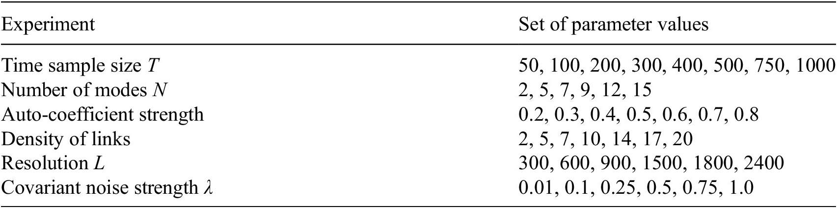
All experiments followed the same default parameters setup. The parameter values of the default setup are given in Table 2. For each experiment, we varied only one of the described parameters of the default setup. The set of values of the varying parameters of each sub-experiment is shown in Table 3. For each sub-experiment, we generated and evaluated 250 SAVAR realizations to obtain a CI of the evaluation metric. To evaluate the estimated sensitivity in each SAVAR realization, the absolute error (AE) is calculated as the absolute difference between the actual sensitivity ( $ \alpha $
) and the estimated sensitivity (
$ \alpha $
) and the estimated sensitivity ( $ \hat{\alpha} $
):
$ \hat{\alpha} $
): $ AE\left(\alpha, \hat{\alpha}\right)=\mid \alpha -\hat{\alpha}\mid $
. The final evaluation metric is the mean absolute error (MAE) which is obtained by averaging the AEs across the 250 SAVAR realizations.
$ AE\left(\alpha, \hat{\alpha}\right)=\mid \alpha -\hat{\alpha}\mid $
. The final evaluation metric is the mean absolute error (MAE) which is obtained by averaging the AEs across the 250 SAVAR realizations.
Table 2. Numerical experiments’ default setup
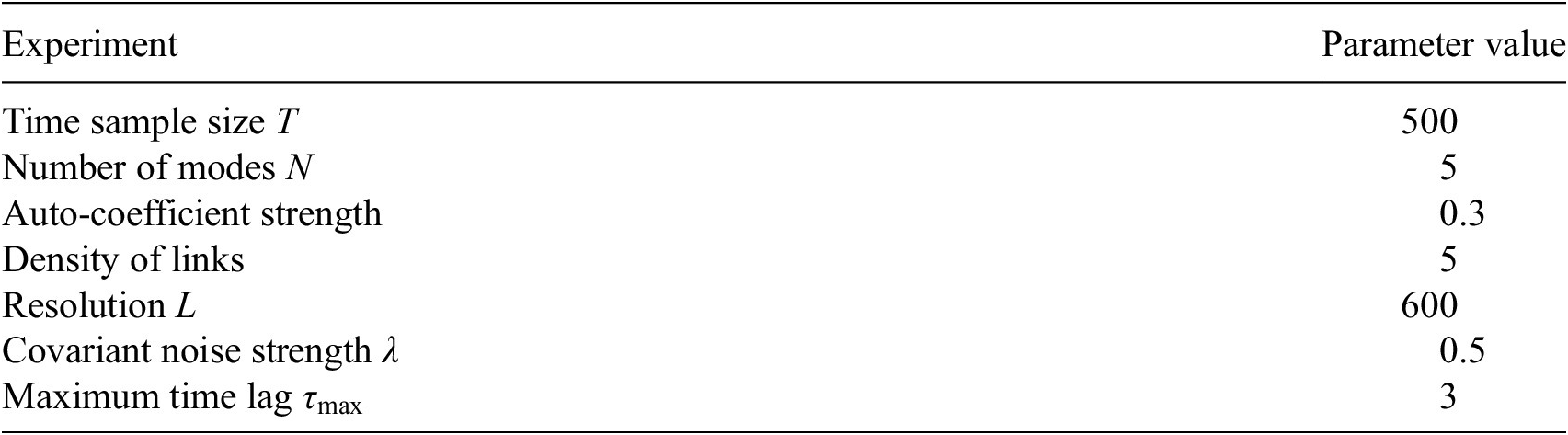
Table 3. Parameters values for Experiment 1
3.1.4. Experimental setup for Experiment 2
In Experiment 2, we compared the different CI methods introduced in Section 3.1.2 for the sensitivity. In addition, to study the effect of the sample size on the different CI methods, we conducted an experiment that follows the default setup of Experiment 1, described in Table 2, in which the sample size varies from $ 100 $
to
$ 100 $
to $ 20000 $
. We generated the synthetic data using 100 random stationary SAVAR models following Equation (2.1). We assumed the true weights
$ 20000 $
. We generated the synthetic data using 100 random stationary SAVAR models following Equation (2.1). We assumed the true weights $ \mathbf{W} $
to be known. The linear coefficient matrices
$ \mathbf{W} $
to be known. The linear coefficient matrices $ \mathbf{A} $
were fitted using VAR estimation or PCMCI–CCM. The sensitivity is then estimated. We calculated the 90% CIs for the five different CI methods. Hundreds of bootstrap realizations were used for the bootstrap-based methods. Like in Experiment 1, we considered the global sensitivity (i.e., the global effects over all small-scale variables) for a uniform and constant unit forcing.
$ \mathbf{A} $
were fitted using VAR estimation or PCMCI–CCM. The sensitivity is then estimated. We calculated the 90% CIs for the five different CI methods. Hundreds of bootstrap realizations were used for the bootstrap-based methods. Like in Experiment 1, we considered the global sensitivity (i.e., the global effects over all small-scale variables) for a uniform and constant unit forcing.
In Experiment 2, we used two evaluation metrics. First, we computed the MAE between the true sensitivity and the estimated sensitivity. This metric measures the ability of the linear coefficient estimation methods—VAR model and PCMCI–CCM—to estimate the sensitivity. Second, we compared the different CI methods by calculating the average size of their 90% CIs.
3.2. Numerical experiments’ results and discussion
3.2.1. Experiment 1 results: Benchmark of estimation methods
In Figure 2, we present the results of Experiment 1. To begin with, we noticed that the Varimax-PCMCI–CCM method performed the best in terms of MAE across a majority of sub-experiments in the benchmark analysis. This superior performance may be attributed to the constraint in Varimax-PCMCI–CCM, where linear coefficients are limited to only causal dependencies identified by PCMCI. This constraint helps prevent the inclusion of spurious linear coefficients, which could otherwise propagate when calculating the sensitivity. Another point to consider is the overlap of the orange and red lines in most sub-experiments. This indicates that using PCA or Varimax had little effect on the average MAE when employing VAR estimation. However, when using PCMCI–CCM to estimate the linear coefficients, Varimax consistently yielded lower MAE compared to PCA across all sub-experiments. Furthermore, we examined the influence of various parameters on the MAE, as shown in Figure 2. Across all methods, we made the following observations:
-
• Increasing the time sample size reduces the average MAE. Larger time sample sizes generally lead to better estimation of linear coefficients, resulting in improved sensitivity estimation.
-
• Increasing the number of modes tends to increase MAE. This effect becomes more pronounced for larger numbers of modes (above 7), although it is less clear for smaller numbers of modes.
-
• Increasing the number of cross-links increases MAE. As cross-links increase, more dependencies emerge, leading to greater error in linear coefficient estimation and subsequently increased AE of the sensitivity.
-
• Increasing the autocorrelation strength increases MAE. Higher autocorrelation can complicate the disentanglement of dependencies and the quantification of linear relationships, resulting in an increased MAE of the sensitivity.
-
• Increasing the spatial resolution decreases MAE. Higher spatial resolution reduces the proportion of points influencing each other due to a constant mode size, thereby decreasing MAE of the sensitivity.
-
• Increasing the covariant noise strength decreases MAE. The covariant noise strength quantifies the contribution of each noise source. Higher covariant noise strength emphasizes the contribution of the mode-level noise, aiding in the estimation of the weights from PCA and Varimax, and consequently leading to a smaller MAE of the sensitivity.
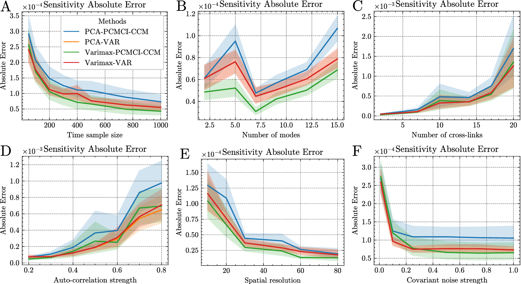
Figure 2. Comparison of four methods to estimate the sensitivity mentioned in Section 3.1.1. The subfigures illustrate how the evaluation metrics (y-axis) vary for the different methods evaluated based on the (A) number of time samples available, (B) number of modes, (C) number of links between the modes, (D) strength of the autocorrelation of each mode, (E) resolution of the spatial grid, and (F) covariant noise strength. The evaluation metric considered is the absolute error (AE) between the ground truth and estimated sensitivity. The mean absolute error (MAE) is represented by the solid lines, and the shaded areas depict the 90% range of the AE metric across the 250 realizations.
The benchmark analysis results for the LREs are depicted in Figure B1 of the Appendix B. Similar trends to those observed in the sensitivity experiment were noted. Specifically, the Varimax-PCMCI–CCM method notably outperformed other methods in achieving the lowest mean relative absolute error for the LREs.
3.2.2. Experiment 2 results: Comparison of CIs
In Figure 3, we present the MAE of the sensitivity estimation using PCMCI–CCM and VAR estimation across varying time sample sizes (100; 500; 1000; 5000; 10,000; 20,000). The green curve shows the MAE of PCMCI–CCM, consistently below the red curve of the VAR estimation. Across all time sample sizes, the MAE is lower with PCMCI–CCM compared to the VAR estimation. This finding supports the results of the preceding experiment where PCMCI–CCM demonstrated superior performance over the VAR method in terms of MAE for sensitivity estimation. We noted a rapid decrease in MAE for PCMCI–CCM and VAR estimation for time sample sizes below 5000. For larger time sample sizes, the MAE gradually approached zero.
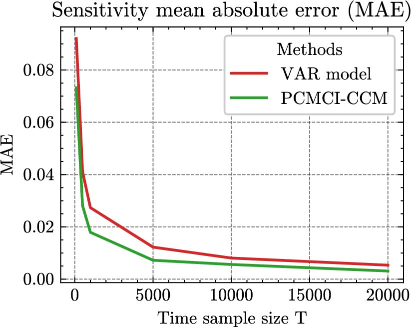
Figure 3. Mean absolute error between true sensitivity and estimated sensitivity. True weights are known and the linear coefficient matrices are estimated with PCMCI–CCM or a VAR model. The Mean Absolute error is averaged over 100 random SAVAR models.
In Figure 4, we plot the average size of the 90% CIs of the sensitivity across 100 random SAVAR-generated models, utilizing the four different bootstrap methods and the asymptotic-based method. VAR estimation is used to estimate the linear coefficient matrix of the SAVAR model in Figure 4A. PCMCI–CCM is used to estimate the linear coefficient of the SAVAR model in Figure 4B. As an example, we also plot the 90% CIs of the sensitivity estimated with PCMCI–CCM and VAR estimation for one of the 100 SAVAR-generated models in Figure 6. In Figure 4A, we found that the average CI size for the VAR estimation is comparable among the five CI methods, except in the case of a time sample size of 100, where the COV-Hall and COV-Standard bootstrap methods exhibit larger CI magnitudes In Figure 4B, we found that the average CI sizes of the asymptotic-based method are larger compared to those obtained through bootstrap-based methods. When comparing Figure 4A,B, we noticed that the average CI size for PCMCI–CCM tended to be smaller than that for VAR estimation.
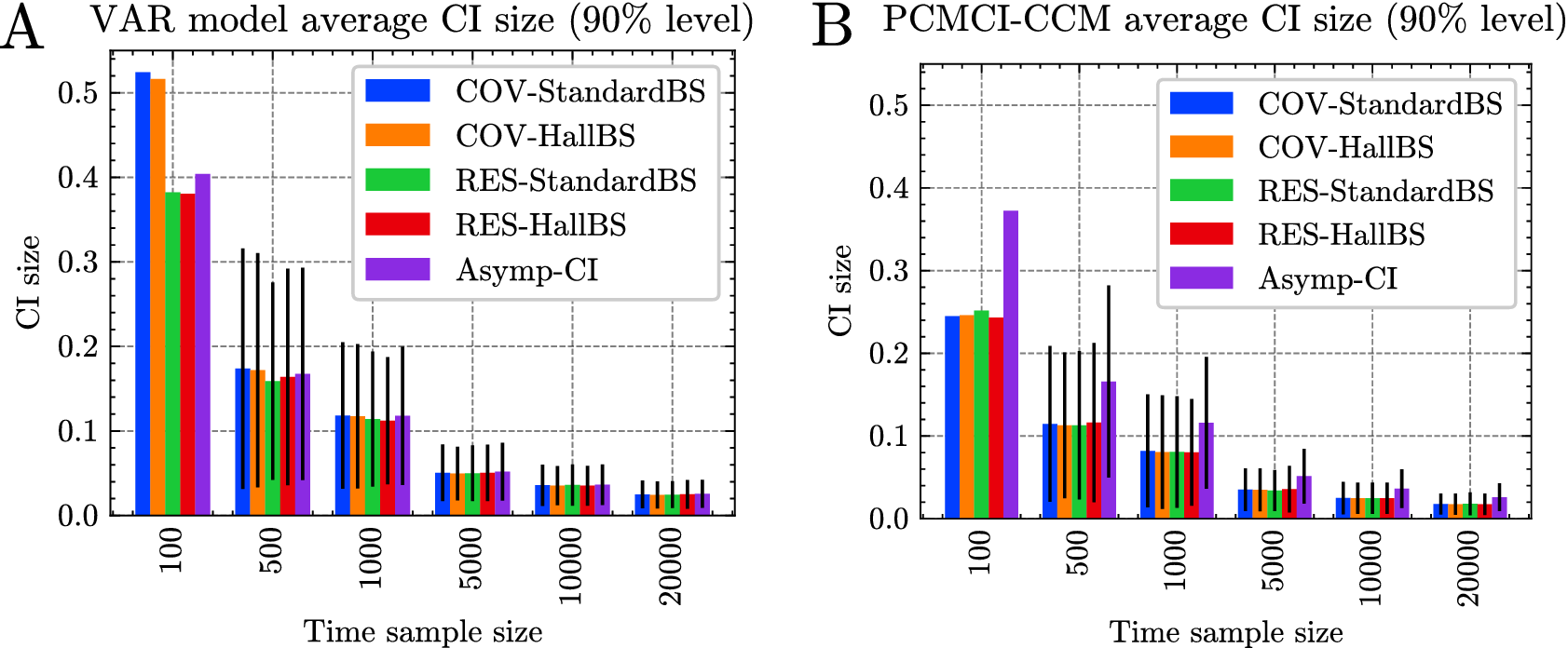
Figure 4. Average CI size of the sensitivity for five different CI methods. Bootstrap-based confidence intervals are computed over 100 bootstrap realizations. The average CI sizes are calculated over the same 100 random SAVAR models of Figure 3. The true weights are known but the linear coefficient matrices are estimated with (A) a VAR model or (B) PCMCI–CCM. To provide an estimation of the variability of the CI size, black error bars indicate the one standard deviation of the CI size over the 100 SAVAR models.
However, it remained unclear to us whether smaller CI sizes were preferable, given that a smaller CI size might be under-conservative. To address this, we assessed the empirical significance level of the 90% CIs. Theoretically, the analytical sensitivity should fall within the 90% CI range with a probability of 90%. To verify this in practice, we calculated the empirical significance level as the frequency of analytical sensitivity falling within the 90% CIs across 100 SAVAR-generated models. The results are depicted in Figure 5. For the VAR model (see Figure 5A), the empirical significance levels closely aligned with the expected 90% level when the time sample size was 1000 or larger. However, for time sample sizes of 100 and 500, the RES-Standard, RES-Hall, and asymptotic CI methods produced overly narrow CIs, resulting in empirical significance levels smaller than expected. For PCMCI–CCM (see Figure 5B), the CI sizes generally appeared well-calibrated, with empirical significance levels closely approximating the 90% level. Nevertheless, it was observed that for a time sample size of 100, all four bootstrap-based CI methods yielded under-conservative CIs, leading to empirical significance levels around 75%, well below the desired 90% level. The asymptotic-based CI exhibited an empirical significance level closer to 90% for this time sample size of 100. However, for larger time sample sizes, the asymptotic CIs tended to be over-conservative, as evidenced by their empirical significance levels surpassing the 90% threshold.
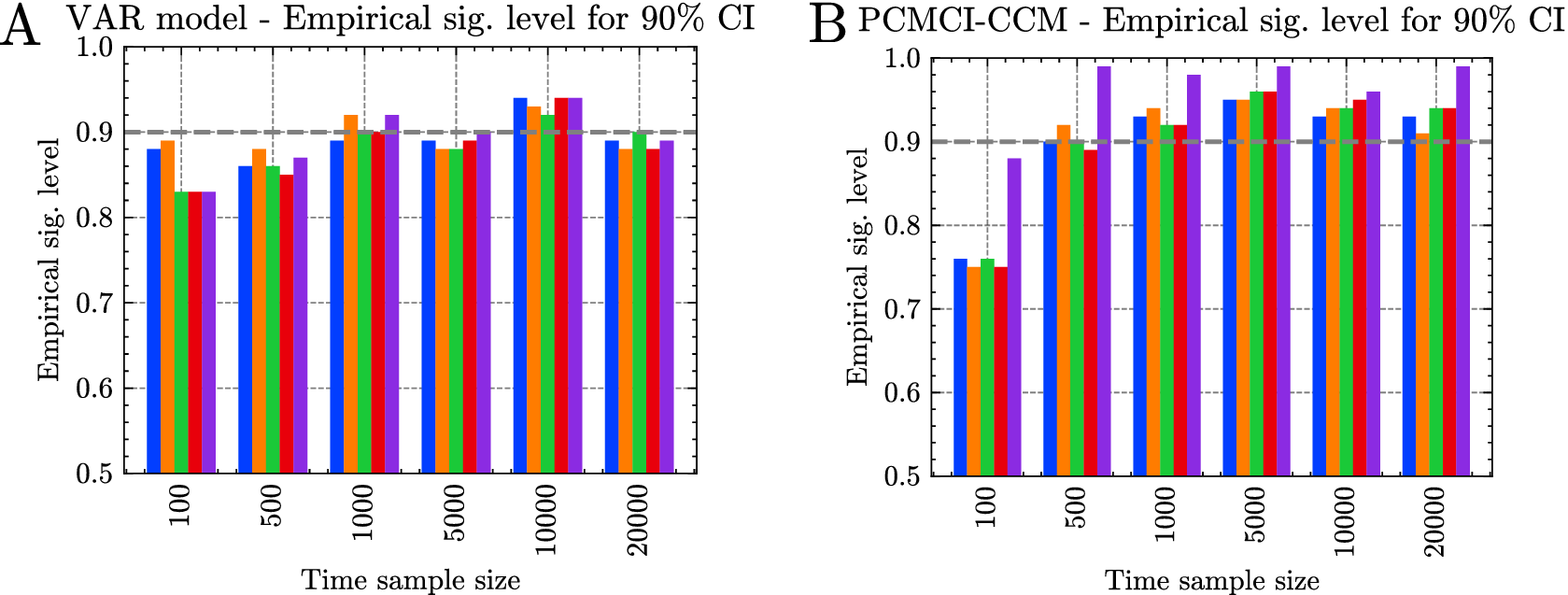
Figure 5. Empirical significance level for the 90% CI shown in Figure 4, for (A) a VAR model or (B) PCMCI–CCM. For each CI method, the empirical significance level is calculated as the frequency of the confidence interval containing the true sensitivity across 100 random SAVAR models. The gray dashed line indicates the 90% significant level. The colormap used in this plot is the same as the one used in Figure 4.
In general, all the bootstrap-based methods yielded comparable CI sizes. This observation applied to PCMCI–CCM and VAR estimation. We attribute the similarity between the CIs of the COV and RES methods to the synthetic data noise, which is characterized by clean Gaussian noises. Consequently, resampling of the residuals or sampling from the covariance matrix of the residuals did not substantially impact the results. Similarly, the Hall and Standard percentile approaches generated similar CIs.
Finally, for PCMCI–CCM, we found that the asymptotic-based approach resulted in wider CIs compared to the bootstrap-based approaches. We think that a possible explanation for the broader asymptotic CIs with PCMCI–CCM is that the variance of the LREs is more likely to be zero because of the constraining of the coefficient by PCMCI. Previous studies by Lütkepohl (Reference Lütkepohl and Lütkepohl2005) and Benkwitz et al. (Reference Benkwitz, Lutkepohl and Neumann1997) have shown that zero coefficients in the variance matrix contribute to more conservative CIs for VAR models. This phenomenon appears to extend to sensitivity CIs as well.
In Figure 6, the CIs were calculated for one particular SAVAR-generated model (the 13th seed). Results for the 12th seed are also shown in Figure B2 of the Appendix B. We found that the estimated sensitivity was slowly converging to the analytical sensitivity, while the CIs became narrower as the time sample size increased. For PCMCI–CCM, the asymptotic-based CIs were wider than the bootstrap-based CIs. For a VAR model, the five CI methods gave very comparable CIs for a time sample size larger than 1000. This aligns with the findings regarding the average size of CIs of Figure 6.
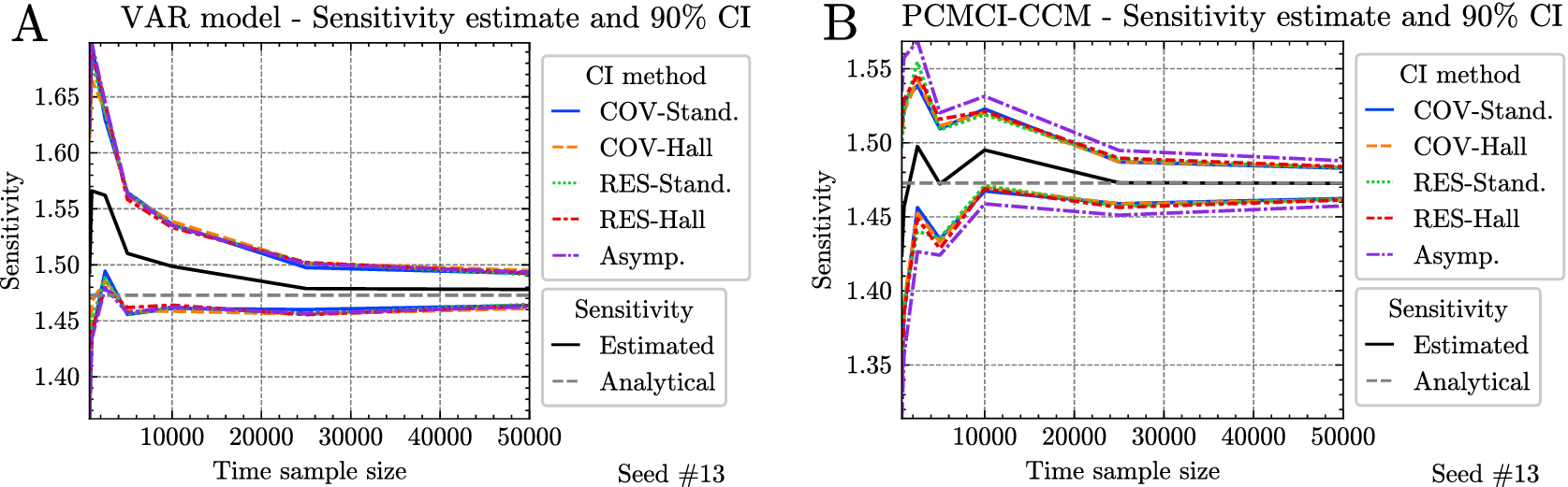
Figure 6. Comparison of the CI methods mentioned in Section 3.1.2 to build a confidence interval of the sensitivity ( $ y $
-axis) for varying time sample size (
$ y $
-axis) for varying time sample size ( $ x $
-axis) for one particular realization of an SAVAR model (seed 13). We plot the 90% CI for five different methods indicated in the legend. The analytical sensitivity is known and indicated by the gray dashed line. The estimated sensitivity is given by the black solid line. To estimate the sensitivity, we used the ground truth mode weights and the linear coefficient matrix estimated with VAR estimation (A) or with PCMCI–CCM (B). The different bootstrap-based confidence intervals are obtained with 100 bootstrap realizations. We calculated the asymptotic-based 90% CI using 1.645 standard deviations of the asymptotic normal distribution.
$ x $
-axis) for one particular realization of an SAVAR model (seed 13). We plot the 90% CI for five different methods indicated in the legend. The analytical sensitivity is known and indicated by the gray dashed line. The estimated sensitivity is given by the black solid line. To estimate the sensitivity, we used the ground truth mode weights and the linear coefficient matrix estimated with VAR estimation (A) or with PCMCI–CCM (B). The different bootstrap-based confidence intervals are obtained with 100 bootstrap realizations. We calculated the asymptotic-based 90% CI using 1.645 standard deviations of the asymptotic normal distribution.
Finally, one noticeable advantage of the asymptotic-based approach is the shorter computational time. Based on our observations from this synthetic experiment, we advocate employing two distinct approaches: a bootstrap-based approach and the asymptotic-based approach to construct CIs with PCMCI–CCM, facilitating a comparative analysis of their outcomes.
3.3. Real-world application
Ideally, we would like to have a real-world dataset for which we know the ground truth LREs and sensitivity. However, such a dataset is not available. Thus, we have opted to examine the long-term effects of two economic variables on $ {\mathrm{NO}}_2 $
pollution in northern Italy. This is guided by the former study of Bichler and Bittner (Reference Bichler and Bittner2022), which found that a decrease in economic activities due to economic crises led to a decrease of
$ {\mathrm{NO}}_2 $
pollution in northern Italy. This is guided by the former study of Bichler and Bittner (Reference Bichler and Bittner2022), which found that a decrease in economic activities due to economic crises led to a decrease of $ {\mathrm{NO}}_2 $
in northern Italy. Our analysis will help to quantify the long-term effects of economic activities on
$ {\mathrm{NO}}_2 $
in northern Italy. Our analysis will help to quantify the long-term effects of economic activities on $ {\mathrm{NO}}_2 $
pollution at the level of the spatial grid (small-scale variables
$ {\mathrm{NO}}_2 $
pollution at the level of the spatial grid (small-scale variables $ {\mathbf{y}}_i $
). In the following section, we introduce the different variables included in our analysis. We then summarize the different steps of the analysis. Finally, we present the estimated LREs of the two economic variables on
$ {\mathbf{y}}_i $
). In the following section, we introduce the different variables included in our analysis. We then summarize the different steps of the analysis. Finally, we present the estimated LREs of the two economic variables on $ {\mathrm{NO}}_2 $
. We also compare statistically significant LREs obtained with the asymptotic-based method and a bootstrap-based method at the level of the spatial grid.
$ {\mathrm{NO}}_2 $
. We also compare statistically significant LREs obtained with the asymptotic-based method and a bootstrap-based method at the level of the spatial grid.
3.3.1. Data
Tropospheric NO2 satellite observations $ {\mathrm{NO}}_2 $
is mainly produced by fossil fuel combustion and therefore primarily caused by anthropogenic processes such as traffic or heating houses during winter. In contrast to ground-based measurements, which can only observe the development of pollutants in a certain area, satellite observations have the advantage of delivering global and self-consistent recordings of air pollutants. In this case, we use tropospheric vertical column densities that which represent the amount of
$ {\mathrm{NO}}_2 $
is mainly produced by fossil fuel combustion and therefore primarily caused by anthropogenic processes such as traffic or heating houses during winter. In contrast to ground-based measurements, which can only observe the development of pollutants in a certain area, satellite observations have the advantage of delivering global and self-consistent recordings of air pollutants. In this case, we use tropospheric vertical column densities that which represent the amount of $ {\mathrm{NO}}_2 $
molecules in a vertical column of air stretching from the ground to the troposphere. Nevertheless, the satellite observations in this study only present the monthly mean
$ {\mathrm{NO}}_2 $
molecules in a vertical column of air stretching from the ground to the troposphere. Nevertheless, the satellite observations in this study only present the monthly mean $ {\mathrm{NO}}_2 $
pollution with morning observations and do not provide information on pollution levels near the Earth’s surface. We averaged the monthly time series to obtain a quarterly time series to be consistent with the time-frequency of the economic time series.
$ {\mathrm{NO}}_2 $
pollution with morning observations and do not provide information on pollution levels near the Earth’s surface. We averaged the monthly time series to obtain a quarterly time series to be consistent with the time-frequency of the economic time series.
Here, we used satellite observations from four different satellites, including ERS-2/GOME, Envisat/SCIAMACHY, MetOp-A/GOME-2, as well as MetOp-B/GOME-2. In particular, we used a harmonized and self-consistent global data product from Georgoulias et al. (Reference Georgoulias, van der, Stammes, Boersma and Eskes2019), which covers the period from 1996 to 2017. The listed satellite observations present the $ {\mathrm{NO}}_2 $
pollution in the early morning between 09:30 Equatorial crossing time (ECT) and 10:30 ECT. Detailed information about the measurement instruments for GOME can be found in Burrows et al. (Reference Burrows, Weber, Buchwitz, Rozanov, Ladstätter-Weißenmayer, Richter, DeBeek, Hoogen, Bramstedt, Eichmann, Eisinger and Perner1999), for SCIAMACHY in Burrows et al. (Reference Burrows, Hölzle, Goede, Visser and Fricke1995) and Bovensmann et al. (Reference Bovensmann, Burrows, Buchwitz, Frerick, Noël, Rozanov, Chance and Goede1999), and for GOME-2 in Munro et al. (Reference Munro, Lang, Klaes, Poli, Retscher, Lindstrot, Huckle, Lacan, Grzegorski, Holdak, Kokhanovsky, Livschitz and Eisinger2016). The data product is provided by the Tropospheric Emission Monitoring Internet Service (TEMIS) and can be accessed free of charge at www.temis.nl. Further information on the TEMIS data product can be found in Georgoulias et al. (Reference Georgoulias, van der, Stammes, Boersma and Eskes2019) as well as Boersma et al. (Reference Boersma, Eskes and Brinksma2004). The data product consists of monthly mean values with a spatial resolution of 0.25° × 0.25° that we quarterly averaged. As described in Boersma (Reference Boersma2008), the
$ {\mathrm{NO}}_2 $
pollution in the early morning between 09:30 Equatorial crossing time (ECT) and 10:30 ECT. Detailed information about the measurement instruments for GOME can be found in Burrows et al. (Reference Burrows, Weber, Buchwitz, Rozanov, Ladstätter-Weißenmayer, Richter, DeBeek, Hoogen, Bramstedt, Eichmann, Eisinger and Perner1999), for SCIAMACHY in Burrows et al. (Reference Burrows, Hölzle, Goede, Visser and Fricke1995) and Bovensmann et al. (Reference Bovensmann, Burrows, Buchwitz, Frerick, Noël, Rozanov, Chance and Goede1999), and for GOME-2 in Munro et al. (Reference Munro, Lang, Klaes, Poli, Retscher, Lindstrot, Huckle, Lacan, Grzegorski, Holdak, Kokhanovsky, Livschitz and Eisinger2016). The data product is provided by the Tropospheric Emission Monitoring Internet Service (TEMIS) and can be accessed free of charge at www.temis.nl. Further information on the TEMIS data product can be found in Georgoulias et al. (Reference Georgoulias, van der, Stammes, Boersma and Eskes2019) as well as Boersma et al. (Reference Boersma, Eskes and Brinksma2004). The data product consists of monthly mean values with a spatial resolution of 0.25° × 0.25° that we quarterly averaged. As described in Boersma (Reference Boersma2008), the $ {\mathrm{NO}}_2 $
product only considers observations with less than 50% of cloud radiance fraction, which is comparable to a cloud fraction of approximately <20%.
$ {\mathrm{NO}}_2 $
product only considers observations with less than 50% of cloud radiance fraction, which is comparable to a cloud fraction of approximately <20%.
The area of study is shown in Figure 7. It is delimited in the north and northwest by the Alps and in the south by the Apennines. Due to the geographic location and the mountain ranges a basin is formed, which is also known as the Po Valley. The Po is the largest river in northern Italy. It flows into the Adriatic Sea in the east, where the Po Valley opens up. Due to the topography, an accumulation of pollutants such as $ {\mathrm{NO}}_2 $
is present. During winter, temperatures for Milan, for example, reach on average around 2 °C. Furthermore, the winter months are the driest months with the lowest amount of precipitation. In comparison to that, the summer months can reach temperatures of around 24 °C with an increase in precipitation (https://de.climate-data.org/).
$ {\mathrm{NO}}_2 $
is present. During winter, temperatures for Milan, for example, reach on average around 2 °C. Furthermore, the winter months are the driest months with the lowest amount of precipitation. In comparison to that, the summer months can reach temperatures of around 24 °C with an increase in precipitation (https://de.climate-data.org/).

It should be considered that meteorology can have an impact on pollution levels. Strong winds or precipitation can, therefore, lead to a reduction in air pollutants, as the pollutants can be, for example, dispersed or washed out. Subsequently, we used the same data source and area of interest in northern Italy as in Bichler and Bittner (Reference Bichler and Bittner2022); therefore, the statement that meteorology was not the reason for the significant decrease in $ {\mathrm{NO}}_2 $
variability between 2007 and 2013 is still valid. Additionally, heavy cloud coverage can have an impact on the
$ {\mathrm{NO}}_2 $
variability between 2007 and 2013 is still valid. Additionally, heavy cloud coverage can have an impact on the $ {\mathrm{NO}}_2 $
observations as well. Further information regarding the cloud coverage for the area of interest can also be found in Bichler and Bittner (Reference Bichler and Bittner2022).
$ {\mathrm{NO}}_2 $
observations as well. Further information regarding the cloud coverage for the area of interest can also be found in Bichler and Bittner (Reference Bichler and Bittner2022).
Quarterly economic time series
As Bichler and Bittner (Reference Bichler and Bittner2022) point out, a majority of the economic output of Italy is generated in northern Italy (G-Econ Project, 2009). The authors further describe, based on economic data from the World Bank (2023), that the service sector accounts for a large proportion of the generated GDP with around 60%. Closely followed by about 40% by the industry and manufacturing sector, and only a small amount by the agricultural sector. This composition of economic sectors, which together represent the GDP, changes only slightly over the period from 1996 to 2017. Therefore, in this study, we assume that a large part of consumption expenditure and the added value by industry are provided in northern Italy. The economic data are publicly available and thus free of charge at http://dati.istat.it/. The quarterly aggregated data on consumer spending of resident and nonresident households as well as data on the value added by industry is used as economic variables. Both data tables cover a period from 1996 to 2017 for the entire country of Italy.
The consumer spending data can be found in the “National Accounts” table under “Quarterly national accounts” in the subcategory “Final consumption expenditure of households by expenditure item and durability.” Here, we used the calendar-adjusted data on “housing, water, electricity, gas and other fuels.” We shortened the variable name to Final Consumption Expenditure in Housing, Water and Electricity (FCE-HWE). Additionally, the added value by industry can also be found in the “Quarterly national accounts” in the subcategory “Value added by industry.” Within this table, the calendar-adjusted data on “electricity, gas, steam and air conditioning supply, water supply, sewerage, waste management and remediation activities” was kept for our analysis. We shortened the variable name to Value Added by Electricity, Gas [VA-EG], etc.). FCE-HWE and VA-EG are both available quarterly and are provided in millions of Euros with the reference year of 2015. Data within the value added by industry section provide information on the contribution to economic growth whereas the consumption expenditure data gives insights on household consumption expenditure classified of individual consumption according to purpose (COICOP) as well as durability (IstatData, 2023a; 2023b).
3.3.2. Analysis
From the $ {\mathrm{NO}}_2 $
pollution time series and the two economic time series, we estimated the LREs of the economics variables (FCE-HWE and VA-EG) on
$ {\mathrm{NO}}_2 $
pollution time series and the two economic time series, we estimated the LREs of the economics variables (FCE-HWE and VA-EG) on $ {\mathrm{NO}}_2 $
pollution in northern Italy. Here, the LREs quantify the impact of a one standard deviation external forcing in a variable on
$ {\mathrm{NO}}_2 $
pollution in northern Italy. Here, the LREs quantify the impact of a one standard deviation external forcing in a variable on $ {\mathrm{NO}}_2 $
pollution. To estimate the LREs, we chose to use the Varimax-PCMCI–CCM method to estimate the LREs as it appeared to be the best-performing method in the benchmark analysis. The analysis includes the steps in the order listed below:
$ {\mathrm{NO}}_2 $
pollution. To estimate the LREs, we chose to use the Varimax-PCMCI–CCM method to estimate the LREs as it appeared to be the best-performing method in the benchmark analysis. The analysis includes the steps in the order listed below:
-
• We used the PCA-Varimax method to estimate the weights
$ \mathbf{W} $
of the
$ {\mathrm{NO}}_2 $
data product. The weights were calculated using only the spatial time series of air pollution (no economic variables). We kept the first five components which captured close to 90% of the total variance. The choice of five components is based on the criterion of explained variance. Sensitivity analyses with alternative component numbers produced qualitatively similar results. Figure 8 shows the map of loadings of these five components. -
• We detrended and standardized the variance of all the time series: the time series of the first five PCA-Varimax components of the
$ {\mathrm{NO}}_2 $
data product and the time series of the two economic variables. We then tested the stationarity of the time series with an augmented Dickey–Fuller test (MacKinnon, Reference MacKinnon1991, Reference MacKinnon1994). Figure 9 presents the considered time series after de-trending. These seven processes define the large-scale variable
$ {X}_i $
(using the notation of the motivational example). Only the five
$ {\mathrm{NO}}_2 $
processes are mapped on the spatial grid (small-scale variables
$ {\mathbf{y}}_i $
) shown in Figure 8. -
• To account for the strong seasonality of the time series, we have added centered seasonal dummy variables in the model. We estimated the causal dependencies with PCMCI+, which allows for contemporaneous links only from the economic variables to air pollution. In this case, it did not modify the formulas of the LREs. Next, we estimated the linear coefficients of the causal dependencies with the CCM method. Table 4 presents the estimated linear coefficients for the regression of the
$ {\mathrm{NO}}_2 $
components on the two economic variables and three seasonal dummy variables. The linear coefficients for the regression of the economic variables are not shown in the table. -
• We estimated the LREs matrix from the estimated weights and the estimated linear coefficients.
-
• We derived CIs of the LREs and plotted the significant LREs of economic variables on
$ {\mathrm{NO}}_2 $
with the asymptotic-based method and a bootstrap-based method. We have to point out that these CIs only include the uncertainty related to the estimation of the linear coefficients and do not include the uncertainty associated with the estimation of the weight matrix
$ \mathbf{W} $
.


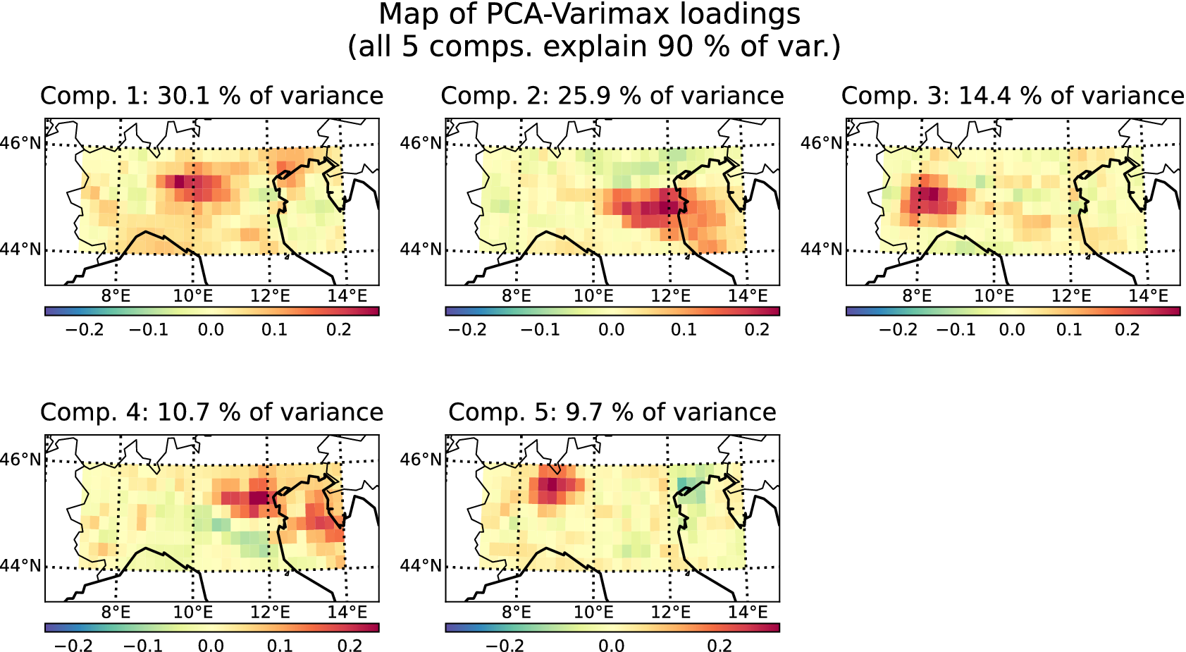
Figure 8. Loadings of the five first PCA-Varimax components of $ {\mathrm{NO}}_2 $
pollution over northern Italy.
$ {\mathrm{NO}}_2 $
pollution over northern Italy.
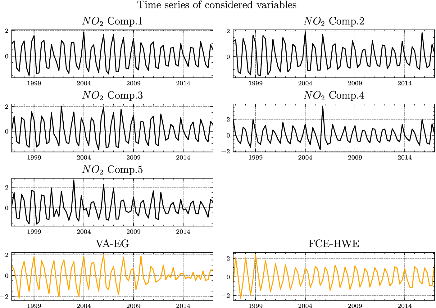
Figure 9. Time series of included variables after linear de-trending. In black solid lines, the time series of the first five PCA-Varimax components of $ {\mathrm{NO}}_2 $
pollution in northern Italy. In orange solid lines, the time series of the two economic variables (VA-EG and FCE-HWE).
$ {\mathrm{NO}}_2 $
pollution in northern Italy. In orange solid lines, the time series of the two economic variables (VA-EG and FCE-HWE).
Table 4. Estimated linear coefficients after the two-step procedure PCMCI+ (selection of causal predictors for each target) and CCM (least squares method to estimate linear dependencies). T-statistics are shown in parentheses. The other values represent the coefficients. All coefficients which are not shown in the table have a value of zero
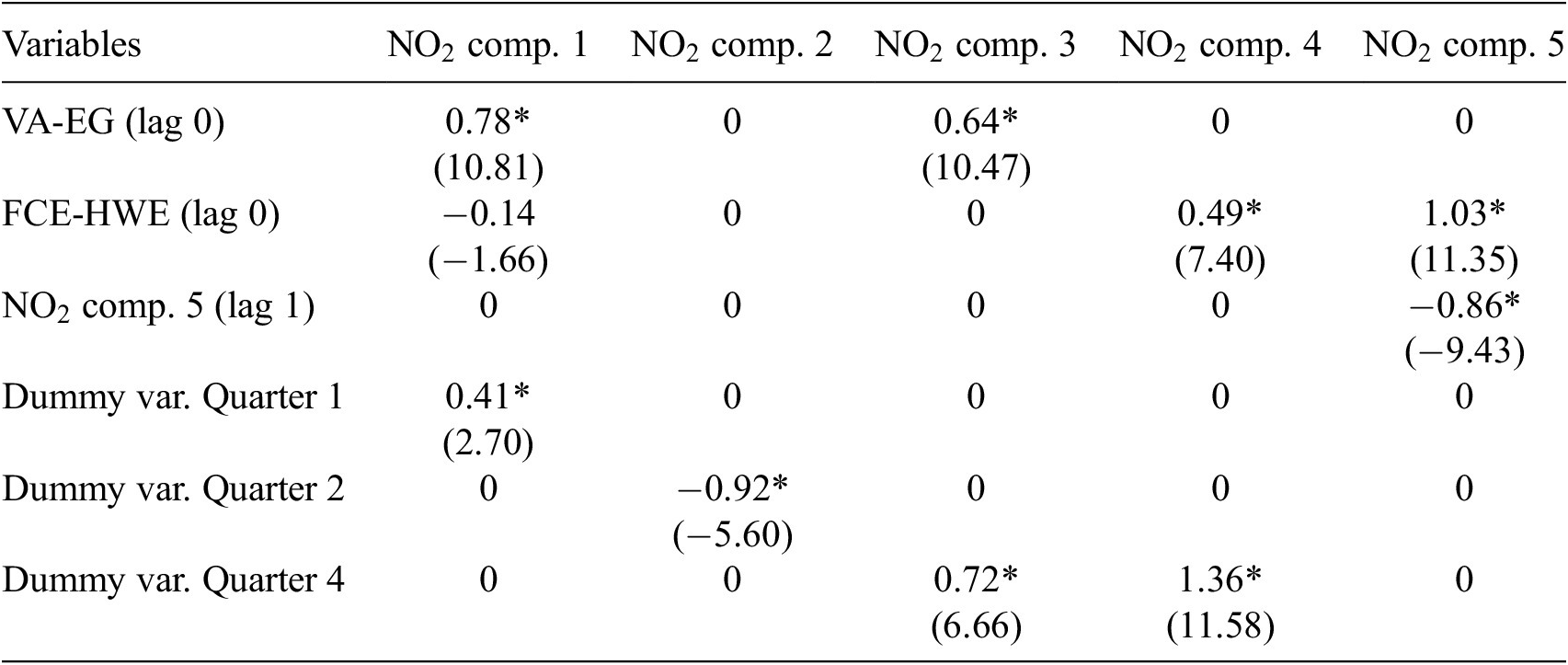
Note: * indicates a p-value $ \le 0.01 $
.
$ \le 0.01 $
.
To avoid the problem of post-selection inference, which arises when the data are used to select the model and introduces additional uncertainty, it is a common practice to use sample splitting (Kuchibhotla et al., Reference Kuchibhotla, Kolassa and Kuffner2022). However, it was not possible to implement sample splitting for this application due to the short available sample size (88 samples).
3.3.3. Results of the real-world application and discussion
Figure 10A,B show the estimated LREs of the two economic variables on $ {\mathrm{NO}}_2 $
pollution, indicating the impact of a one standard deviation change in these variables on
$ {\mathrm{NO}}_2 $
pollution, indicating the impact of a one standard deviation change in these variables on $ {\mathrm{NO}}_2 $
pollution levels. Notably, the sensitivity of VA-EG and FCE-HWE to
$ {\mathrm{NO}}_2 $
pollution levels. Notably, the sensitivity of VA-EG and FCE-HWE to $ {\mathrm{NO}}_2 $
pollution is positive, with VA-EG exhibiting a slightly higher sensitivity (0.04) compared to FCE-HWE (0.02). This indicates a positive effect of economic activity on
$ {\mathrm{NO}}_2 $
pollution is positive, with VA-EG exhibiting a slightly higher sensitivity (0.04) compared to FCE-HWE (0.02). This indicates a positive effect of economic activity on $ {\mathrm{NO}}_2 $
pollution in northern Italy, consistent with prior observations made by Bichler and Bittner (Reference Bichler and Bittner2022). Moreover, using a bootstrap approach, we obtained CIs for the sensitivity, and for a one-sided significance level of 10%, the lower bounds are 0.022 for VA-EG and 0.0026 for FCE-HWE, indicating statistically significant positive values. Our methodology further details the spatial distribution of economic activity’s impact on
$ {\mathrm{NO}}_2 $
pollution in northern Italy, consistent with prior observations made by Bichler and Bittner (Reference Bichler and Bittner2022). Moreover, using a bootstrap approach, we obtained CIs for the sensitivity, and for a one-sided significance level of 10%, the lower bounds are 0.022 for VA-EG and 0.0026 for FCE-HWE, indicating statistically significant positive values. Our methodology further details the spatial distribution of economic activity’s impact on $ {\mathrm{NO}}_2 $
pollution. For example, we can note the more pronounced effects observed in urban areas, with sporadic small negative LREs attributed to minor negative loadings of PCA-Varimax components. Figure 10C,D exhibit the asymptotic statistically significant LREs at a one-sided significance level of 10%. However, only a fraction of these effects reach significance, resulting in a sparse map. In Figure 10E,F, we plot the significant LREs with a one-sided significance level of 10% using the bootstrap-based RES-Standard approach (with 1000 bootstrap realizations). The significance maps reveal that the bootstrap approach identifies more significant effects for VA-EG and FCE-HWE compared to the asymptotic approach. These disparities in significance between asymptotic and bootstrap approaches align with observations from synthetic data experiments (see Section 3.2.2), indicating that asymptotic-based CIs tend to be more conservative. Selecting the optimal approach for this specific analysis remains challenging and would require further investigation.
$ {\mathrm{NO}}_2 $
pollution. For example, we can note the more pronounced effects observed in urban areas, with sporadic small negative LREs attributed to minor negative loadings of PCA-Varimax components. Figure 10C,D exhibit the asymptotic statistically significant LREs at a one-sided significance level of 10%. However, only a fraction of these effects reach significance, resulting in a sparse map. In Figure 10E,F, we plot the significant LREs with a one-sided significance level of 10% using the bootstrap-based RES-Standard approach (with 1000 bootstrap realizations). The significance maps reveal that the bootstrap approach identifies more significant effects for VA-EG and FCE-HWE compared to the asymptotic approach. These disparities in significance between asymptotic and bootstrap approaches align with observations from synthetic data experiments (see Section 3.2.2), indicating that asymptotic-based CIs tend to be more conservative. Selecting the optimal approach for this specific analysis remains challenging and would require further investigation.
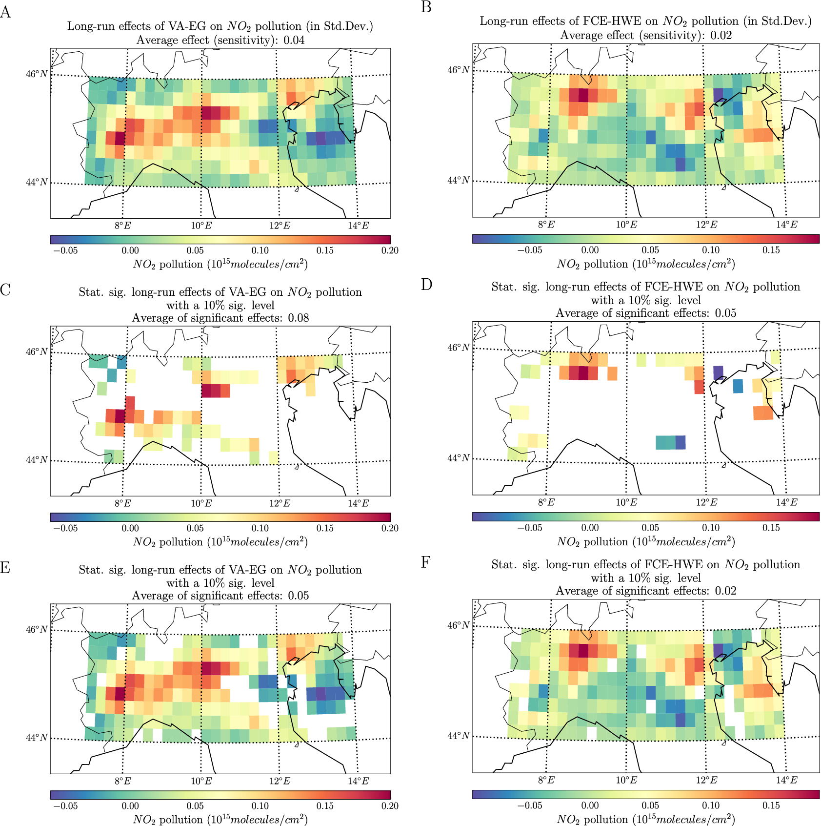
Figure 10. (A) and (B) Long-run effects of economic variables (VA-EG and FCE-HWE) on $ {\mathrm{NO}}_2 $
pollution. (C) and (D) Statistically significant long-run effects of economic variables (VA-EG and FCE-HWE) on
$ {\mathrm{NO}}_2 $
pollution. (C) and (D) Statistically significant long-run effects of economic variables (VA-EG and FCE-HWE) on $ {\mathrm{NO}}_2 $
pollution in northern Italy. Here, the confidence interval is obtained using the asymptotic distribution of the long-run effects and with a one-sided significance level of 10%. (E) and (F) Statistically significant long-run effects of economic variables (VA-EG and FCE-HWE) on
$ {\mathrm{NO}}_2 $
pollution in northern Italy. Here, the confidence interval is obtained using the asymptotic distribution of the long-run effects and with a one-sided significance level of 10%. (E) and (F) Statistically significant long-run effects of economic variables (VA-EG and FCE-HWE) on $ {\mathrm{NO}}_2 $
pollution in northern Italy. Here, the confidence intervals are obtained with a bootstrap of the residuals and Hall’s percentile interval and with a one-sided significance level of 10% and 1000 bootstrap realizations.
$ {\mathrm{NO}}_2 $
pollution in northern Italy. Here, the confidence intervals are obtained with a bootstrap of the residuals and Hall’s percentile interval and with a one-sided significance level of 10% and 1000 bootstrap realizations.
4. Discussion and conclusion
We have tackled the challenge of estimating the effects of perturbations at a small scale within an SAVAR model (see Tibau et al. (Reference Tibau, Reimers, Gerhardus, Denzler, Eyring and Runge2022)). This model incorporates a VAR framework and maps the VAR processes onto smaller-scale variables. We proposed two measures for quantifying the impact of an external perturbation, called forcing, in this model: the LREs, which capture the impact of a unit forcing between each pair of small-scale variables at equilibrium, and the sensitivity, which measures the average effect of a unit forcing on the small-scale variables of interest at equilibrium. Both measures provide insight into the impact of a forcing at the small scale when the system reaches equilibrium, enabling more localized quantification than a standard VAR model would allow. We derived explicit formulas for these measures in an SAVAR model and introduced their estimators. Additionally, we provided the asymptotic distributions of these estimators, which can be used to construct CIs. However, these asymptotic CIs only account for the uncertainty associated with estimating the linear coefficients of an SAVAR model.
Our first numerical experiment compared several methods for estimating sensitivity and LREs using synthetic data across varying SAVAR parameters. In all experiments, the Varimax-PCMCI–CCM method demonstrated better performance on average in terms of MAE compared to methods based on VAR estimation. The superior performance of the Varimax-PCMCI–CCM method likely arises from the enhanced spatial localization achieved through Varimax rotation combined with the improved identification of causally relevant dependencies by PCMCI, which together mitigate the propagation of spurious coefficients. The second numerical experiment focused on comparing bootstrap-based methods with the asymptotic-based method for constructing CIs of sensitivity. On synthetic data, bootstrap-based methods produced narrower CIs than the asymptotic-based method. We applied the estimation of LREs with uncertainty quantification to real-world data, specifically estimating the LREs of two economic activities on $ {\mathrm{NO}}_2 $
pollution in northern Italy at the grid level. Both bootstrap-based and asymptotic-based CIs allowed us to identify statistically significant LREs on
$ {\mathrm{NO}}_2 $
pollution in northern Italy at the grid level. Both bootstrap-based and asymptotic-based CIs allowed us to identify statistically significant LREs on $ {\mathrm{NO}}_2 $
at the grid level, enabling a more localized analysis of the effects of economic activities on air pollution.
$ {\mathrm{NO}}_2 $
at the grid level, enabling a more localized analysis of the effects of economic activities on air pollution.
Our approach does have limitations. First, we assume that all relevant variables are observed and can be included in an SAVAR model. This assumption may limit the practical applications when unobserved variables or variables that cannot be effectively modeled as an SAVAR process are present. Additionally, the methods we used to construct CIs only consider the uncertainty related to the estimation of the linear coefficients and not the uncertainty associated with the estimation of the weights of an SAVAR model when they are also estimated. Accounting for this uncertainty is particularly challenging for the asymptotic distribution of the estimators of the LREs and sensitivity. Future work could involve developing bootstrap methods to estimate both the aggregation weights and the linear coefficients, thereby quantifying both sources of uncertainty simultaneously.
Acknowledgments
The authors are grateful for the technical assistance of Tibau X.-A. The authors would also like to thank the computational resources of the Deutsches Klimarechenzentrum (DKRZ, Hamburg, Germany) used for the numerical experiments and application of the present work. The authors acknowledge the free use of the tropospheric $ {\mathrm{NO}}_2 $
column data from GOME-2B, GOME-2A, SCIAMACHY, and GOME sensor from www.temis.nl. The authors would also like to acknowledge the free use of the economic data from www.istat.it.
$ {\mathrm{NO}}_2 $
column data from GOME-2B, GOME-2A, SCIAMACHY, and GOME sensor from www.temis.nl. The authors would also like to acknowledge the free use of the economic data from www.istat.it.
Data availability statement
The Python code for the synthetic data experiments, and Python code together with the datasets for the real-world application are freely available at github.com/EyringMLClimateGroup/debeire25eds_UncertaintyCausalEffects.
Author contribution
Conceptualization: K.D., V.E., A.G., and J.R. Methodology: K.D. and A.G. Formal analysis: K.D. Supervision: V.E., A.G., and J.R. Software: K.D. Data curation: K.D. and R.B. Writing—original draft: K.D. and R.B. Writing—review and editing: K.D., R.B., V.E., A.G., and J.R.
Funding statement
K.D. and V.E have received funding for this study provided by the European Research Council (ERC) Synergy Grant “Understanding and Modeling the Earth System with Machine Learning (USMILE)” under the Horizon 2020 Research and Innovation Program (Grant Agreement No. 855187). R.B. has been supported by the DLR/DAAD Research Fellowship—Doctoral Studies in Germany, funded by the German Academic Exchange Service (DAAD, No. 57478193). J.R. has received funding from the European Research Council (ERC) Starting Grant CausalEarth under the European Union’s Horizon 2020 research and innovation program (Grant Agreement No. 948112).
Competing interests
The authors declare that no competing interests exist.
A. Appendix
A.1. Derivation of the sensitivity in an SAVAR model
Two equivalent formulas can be derived for the sensitivity in an SAVAR model. We recall the definition of the sensitivity given in Equation (2.3a):
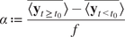 $$ \alpha \hskip0.35em := \hskip0.35em \frac{\overline{\left\langle {\mathbf{y}}_{t\ge {t}_0}\right\rangle }-\overline{\left\langle {\mathbf{y}}_{t<{t}_0}\right\rangle }}{f} $$
where $ \left\langle \mathbf{y}\right\rangle $
denotes the temporal mean of
$ \left\langle \mathbf{y}\right\rangle $
denotes the temporal mean of $ \mathbf{y} $
and
$ \mathbf{y} $
and $ \overline{\mathbf{y}} $
is the mean of
$ \overline{\mathbf{y}} $
is the mean of $ \mathbf{y} $
over the
$ \mathbf{y} $
over the $ L $
points.
$ L $
points.
For $ t<{t}_0 $
, there is no forcing and
$ t<{t}_0 $
, there is no forcing and $ {\mathbf{y}}_t $
has the form:
$ {\mathbf{y}}_t $
has the form:
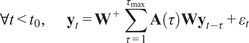 $$ \forall t<{t}_0,\hskip2em {\mathbf{y}}_t={\mathbf{W}}^{+}\sum \limits_{\tau =1}^{\tau_{\mathrm{max}}}\mathbf{A}\left(\tau \right){\mathbf{W}\mathbf{y}}_{t-\tau }+{\varepsilon}_t $$
However for $ t\ge {t}_0 $
, the system is subject to an external forcing
$ t\ge {t}_0 $
, the system is subject to an external forcing $ f $
with forcing weights
$ f $
with forcing weights $ \mathbf{b} $
, such that
$ \mathbf{b} $
, such that $ {\mathbf{y}}_t $
has the form:
$ {\mathbf{y}}_t $
has the form:
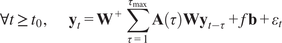 $$ \forall t\ge {t}_0,\hskip2em {\mathbf{y}}_t={\mathbf{W}}^{+}\sum \limits_{\tau =1}^{\tau_{\mathrm{max}}}\mathbf{A}\left(\tau \right){\mathbf{W}\mathbf{y}}_{t-\tau }+f\mathbf{b}+{\varepsilon}_t $$
Derivation of the first explicit formula
The first formula can be derived with the following steps. First, applying the temporal mean 〈〉
![]() and regrouping terms with
and regrouping terms with $ \mathbf{y} $
on the left side yields:
$ \mathbf{y} $
on the left side yields:
 $$ \forall t<{t}_0,\hskip2em \left\langle {\mathbf{y}}_t\right\rangle -{\mathbf{W}}^{+}\sum \limits_{\tau =1}^{\tau_{\mathrm{max}}}\;\mathbf{A}\left(\tau \right)\mathbf{W}\left\langle {\mathbf{y}}_{t-\tau}\right\rangle =\left\langle {\varepsilon}_t\right\rangle $$
 $$ \forall t\ge {t}_0,\hskip2em \left\langle {\mathbf{y}}_t\right\rangle -{\mathbf{W}}^{+}\sum \limits_{\tau =1}^{\tau_{\mathrm{max}}}\;\mathbf{A}\left(\tau \right)\mathbf{W}\left\langle {\mathbf{y}}_{t-\tau}\right\rangle =f\mathbf{b}+\left\langle {\varepsilon}_t\right\rangle $$
We now show that the pre-forcing period and the post-forcing equilibrium are stationary periods so that $ \left\langle {\mathbf{y}}_t\right\rangle =\left\langle {\mathbf{y}}_{t-\tau}\right\rangle $
for
$ \left\langle {\mathbf{y}}_t\right\rangle =\left\langle {\mathbf{y}}_{t-\tau}\right\rangle $
for $ t\ge {t}_0 $
and
$ t\ge {t}_0 $
and $ t<{t}_0 $
. For the pre-forcing period, we assume that the SAVAR model is stable. For the post-forcing equilibrium, the SAVAR model is stable and the system is in a state of equilibrium. In addition, the process is also stable for nonzero mean noise terms
$ t<{t}_0 $
. For the pre-forcing period, we assume that the SAVAR model is stable. For the post-forcing equilibrium, the SAVAR model is stable and the system is in a state of equilibrium. In addition, the process is also stable for nonzero mean noise terms $ {\varepsilon}_t $
and nonzero forcing
$ {\varepsilon}_t $
and nonzero forcing $ {f}_t $
.
$ {f}_t $
.
For a stationary time period, we have $ \left\langle {\mathbf{y}}_t\right\rangle =\left\langle {\mathbf{y}}_{t-\tau}\right\rangle $
, and it follows:
$ \left\langle {\mathbf{y}}_t\right\rangle =\left\langle {\mathbf{y}}_{t-\tau}\right\rangle $
, and it follows:
 $$ \forall t<{t}_0,\hskip2em \left\langle {\mathbf{y}}_t\right\rangle \left({I}_L-{\mathbf{W}}^{+}\sum \limits_{\tau =1}^{\tau_{\mathrm{max}}}\;\mathbf{A}\left(\tau \right)\mathbf{W}\right)=\left\langle {\varepsilon}_t\right\rangle $$
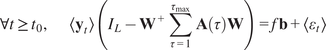 $$ \forall t\ge {t}_0,\hskip2em \left\langle {\mathbf{y}}_t\right\rangle \left({I}_L-{\mathbf{W}}^{+}\sum \limits_{\tau =1}^{\tau_{\mathrm{max}}}\;\mathbf{A}\left(\tau \right)\mathbf{W}\right)=f\mathbf{b}+\left\langle {\varepsilon}_t\right\rangle $$
Under our assumption that $ {\mathbf{y}}_t $
is a stable SAVAR process, the matrix
$ {\mathbf{y}}_t $
is a stable SAVAR process, the matrix $ \left({I}_L-{\mathbf{W}}^{+}{\sum}_{\tau =1}^{\tau_{\mathrm{max}}}\mathbf{A}\left(\tau \right)\mathbf{W}\right) $
is invertible:
$ \left({I}_L-{\mathbf{W}}^{+}{\sum}_{\tau =1}^{\tau_{\mathrm{max}}}\mathbf{A}\left(\tau \right)\mathbf{W}\right) $
is invertible:
 $$ \forall t<{t}_0,\hskip2em \left\langle {\mathbf{y}}_t\right\rangle ={\left({I}_L-{\mathbf{W}}^{+}\sum \limits_{\tau =1}^{\tau_{\mathrm{max}}}\;\mathbf{A}\left(\tau \right)\mathbf{W}\right)}^{-1}\left\langle {\varepsilon}_t\right\rangle $$
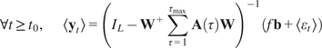 $$ \forall t\ge {t}_0,\hskip2em \left\langle {\mathbf{y}}_t\right\rangle ={\left({I}_L-{\mathbf{W}}^{+}\sum \limits_{\tau =1}^{\tau_{\mathrm{max}}}\;\mathbf{A}\left(\tau \right)\mathbf{W}\right)}^{-1}\left(f\mathbf{b}+\left\langle {\varepsilon}_t\right\rangle \right) $$
We can finally substitute the derived $ \left\langle {y}_{t>{t}_0}\right\rangle $
and
$ \left\langle {y}_{t>{t}_0}\right\rangle $
and $ \left\langle {y}_{t<{t}_0}\right\rangle $
in the definition of the sensitivity to obtain:
$ \left\langle {y}_{t<{t}_0}\right\rangle $
in the definition of the sensitivity to obtain:
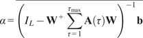 $$ \alpha =\overline{{\left({I}_L-{\mathbf{W}}^{+}\sum \limits_{\tau =1}^{\tau_{\mathrm{max}}}\mathbf{A}\left(\tau \right)\mathbf{W}\right)}^{-1}\mathbf{b}} $$
Yielding the first explicit formula of Equation (2.3b):
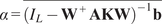 $$ \alpha =\overline{{\left({I}_L-{\mathbf{W}}^{+}\mathbf{AKW}\right)}^{-1}\mathbf{b}} $$
Derivation of the second explicit formula
The second formula results from noticing that $ {\mathbf{W}}^{+}\mathbf{W} $
is a projection. Hence,
$ {\mathbf{W}}^{+}\mathbf{W} $
is a projection. Hence, $ {\mathbf{y}}_t $
can be decomposed uniquely as the sum of two terms, one belonging to
$ {\mathbf{y}}_t $
can be decomposed uniquely as the sum of two terms, one belonging to $ \mathit{\operatorname{Im}}\left({\mathbf{W}}^{+}\mathbf{W}\right) $
and the other belonging to
$ \mathit{\operatorname{Im}}\left({\mathbf{W}}^{+}\mathbf{W}\right) $
and the other belonging to $ \mathit{\operatorname{Ker}}\left({\mathbf{W}}^{+}\mathbf{W}\right) $
:
$ \mathit{\operatorname{Ker}}\left({\mathbf{W}}^{+}\mathbf{W}\right) $
:
 $$ {\mathbf{y}}_t=\left({I}_L-{\mathbf{W}}^{+}\mathbf{W}\right){\mathbf{y}}_t+{\mathbf{W}}^{+}{\mathbf{W}\mathbf{y}}_t $$
We can in turn decompose $ \alpha $
:
$ \alpha $
:
 $$ f\alpha =\overline{\left({I}_L-{\mathbf{W}}^{+}\mathbf{W}\right)\left(\left\langle {\mathbf{y}}_{t\ge {t}_0}\right\rangle -\left\langle {\mathbf{y}}_{t<{t}_0}\right\rangle \right)+{\mathbf{W}}^{+}\mathbf{W}\left(\left\langle {\mathbf{y}}_{t\ge {t}_0}\right\rangle -\left\langle {\mathbf{y}}_{t<{t}_0}\right\rangle \right)} $$
For the first term, one can find that:
 $$ \left({I}_L-{\mathbf{W}}^{+}\mathbf{W}\right)\left(\left\langle {\mathbf{y}}_{t\ge {t}_0}\right\rangle -\left\langle {\mathbf{y}}_{t<{t}_0}\right\rangle \right)=\left({I}_L-{\mathbf{W}}^{+}\mathbf{W}\right)f\mathbf{b} $$
For the second term, we first apply the definition of $ \mathbf{x} $
:
$ \mathbf{x} $
:
 $$ {\mathbf{W}}^{+}\mathbf{W}\left(\left\langle {\mathbf{y}}_{t\ge {t}_0}\right\rangle -\left\langle {\mathbf{y}}_{t<{t}_0}\right\rangle \right)={\mathbf{W}}^{+}\left(\left\langle {\mathbf{x}}_{t\ge {t}_0}\right\rangle -\left\langle {\mathbf{x}}_{t<{t}_0}\right\rangle \right) $$
Under our assumption that $ {\mathbf{x}}_t $
is a stable VAR process, the matrix
$ {\mathbf{x}}_t $
is a stable VAR process, the matrix $ \left({I}_N- AK\right) $
is invertible, we have:
$ \left({I}_N- AK\right) $
is invertible, we have:
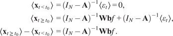 $$ {\displaystyle \begin{array}{c}\left\langle {\mathbf{x}}_{t<{t}_0}\right\rangle ={\left({I}_N-\mathbf{A}\right)}^{-1}\left\langle {\varepsilon}_t\right\rangle =0,\\ {}\left\langle {\mathbf{x}}_{t\ge {t}_0}\right\rangle ={\left({I}_N-\mathbf{A}\right)}^{-1}\mathbf{Wb}f+{\left({I}_N-\mathbf{A}\right)}^{-1}\left\langle {\varepsilon}_t\right\rangle, \\ {}\left\langle {\mathbf{x}}_{t\ge {t}_0}\right\rangle -\left\langle {\mathbf{x}}_{t<{t}_0}\right\rangle ={\left({I}_N-\mathbf{A}\right)}^{-1}\mathbf{Wb}f.\end{array}} $$
This yields the second term:
 $$ {\mathbf{W}}^{+}\mathbf{W}\left(\left\langle {\mathbf{y}}_{t\ge {t}_0}\right\rangle -\left\langle {\mathbf{y}}_{t<{t}_0}\right\rangle \right)={\mathbf{W}}^{+}{\left({I}_N-\mathbf{AK}\right)}^{-1}\mathbf{W}\mathbf{b}f $$
Finally, combining the two derived terms yields the second explicit formula given in Equation (2.3c):
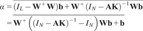 $$ {\displaystyle \begin{array}{c}\alpha =\overline{\left({I}_L-{\mathbf{W}}^{+}\mathbf{W}\right)\mathbf{b}+{\mathbf{W}}^{+}{\left({I}_N-\mathbf{AK}\right)}^{-1}\mathbf{W}\mathbf{b}}\\ {}=\overline{{\mathbf{W}}^{+}\left({\left({I}_N-\mathbf{AK}\right)}^{-1}-{I}_N\right)\mathbf{Wb}+\mathbf{b}}\end{array}} $$
A.2. Notations and useful propositions and rules
We denote with $ vec $
the vectorization of a matrix, which converts the matrix into a column vector. Specifically, the vectorization of a
$ vec $
the vectorization of a matrix, which converts the matrix into a column vector. Specifically, the vectorization of a $ m\times n $
matrix
$ m\times n $
matrix $ \mathbf{A} $
, denoted
$ \mathbf{A} $
, denoted $ vec\left(\mathbf{A}\right) $
, is the
$ vec\left(\mathbf{A}\right) $
, is the $ mn\times 1 $
column vector obtained by stacking the columns of the matrix
$ mn\times 1 $
column vector obtained by stacking the columns of the matrix $ \mathbf{A} $
on top of one another. The Kronecker product is represented by the symbol
$ \mathbf{A} $
on top of one another. The Kronecker product is represented by the symbol $ \otimes $
. We will derive the asymptotic distributions of the estimators thanks to the following propositions.
$ \otimes $
. We will derive the asymptotic distributions of the estimators thanks to the following propositions.
Proposition A.1. (Delta method).
Suppose $ \beta $
is an
$ \beta $
is an $ \left(n\times 1\right) $
vector of parameters and
$ \left(n\times 1\right) $
vector of parameters and $ \hat{\beta} $
is an estimator such that.
$ \hat{\beta} $
is an estimator such that.
 $$ \sqrt{T}\left(\hat{\beta}-\beta \right)\overset{d}{\to}\mathcal{N}\left(0,{\boldsymbol{\Sigma}}_{\hat{\beta}}\right) $$
where $ T $
denotes the sample size used for estimation. Denoting by ′ the transpose and for a vector-valued continuously differentiable function
$ T $
denotes the sample size used for estimation. Denoting by ′ the transpose and for a vector-valued continuously differentiable function $ g $
with
$ g $
with $ \frac{\partial g}{\partial {\beta}^{\prime }}\ne 0 $
at
$ \frac{\partial g}{\partial {\beta}^{\prime }}\ne 0 $
at $ \beta $
, we have:
$ \beta $
, we have:
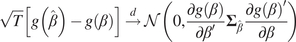 $$ \sqrt{T}\left[g\left(\hat{\beta}\right)-g\left(\beta \right)\right]\overset{d}{\to}\mathcal{N}\left(0,\frac{\partial g\left(\beta \right)}{\partial {\beta}^{\prime }}{\boldsymbol{\Sigma}}_{\hat{\beta}}\frac{\partial g{\left(\beta \right)}^{\prime }}{\partial \beta}\right) $$ $ \square $
Proposition A.2. (Derivation rules of vec(.), see Lütkepohl (Reference Lütkepohl and Lütkepohl2005), Appendix A.13).
 $$ \frac{\partial vec\;\left(\mathbf{AB}\left(\beta \right)\mathbf{C}\right)}{\partial {\beta}^{\prime }}=\left({\mathbf{C}}^{\prime}\hskip0.5em \otimes \hskip0.5em \mathbf{A}\right)\frac{\partial vec\left(\mathbf{B}\right)}{\partial {\beta}^{\prime }} $$
 $$ \frac{\partial vec\left({\mathbf{A}}^{-1}\right)}{\partial vec{\left(\mathbf{A}\right)}^{\prime }}=-{\left({\mathbf{A}}^{-1}\right)}^{\prime}\hskip0.5em \otimes \hskip0.5em {\mathbf{A}}^{-1} $$
A.3. Asymptotic distributions of the estimators of the LREs and of the sensitivity
We can now apply the propositions given in Appendix A.2 to derive the asymptotic distributions of $ {\hat{\boldsymbol{\Psi}}}_{\infty } $
and
$ {\hat{\boldsymbol{\Psi}}}_{\infty } $
and $ \hat{\alpha} $
.
$ \hat{\alpha} $
.
Proposition A.3. (Asymptotic distribution of $ {\hat{\boldsymbol{\Psi}}}_{\infty } $
).
$ {\hat{\boldsymbol{\Psi}}}_{\infty } $
).
We keep the definition of $ {\boldsymbol{\Psi}}_{\infty } $
given in Equations (2.4a) and (2.4b).
$ {\boldsymbol{\Psi}}_{\infty } $
given in Equations (2.4a) and (2.4b).
We note $ \hat{\beta}= vec\left(\hat{\mathbf{A}}\right) $
and
$ \hat{\beta}= vec\left(\hat{\mathbf{A}}\right) $
and $ \beta = vec\left(\mathbf{A}\right) $
.
$ \beta = vec\left(\mathbf{A}\right) $
.
If
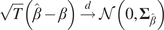 $$ \sqrt{T}\left(\hat{\beta}-\beta \right)\overset{d}{\to}\mathcal{N}\left(0,{\boldsymbol{\Sigma}}_{\hat{\beta}}\right) $$
Then
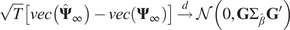 $$ \sqrt{T}\left[ vec\left({\hat{\boldsymbol{\Psi}}}_{\infty}\right)- vec\left({\boldsymbol{\Psi}}_{\infty}\right)\right]\overset{d}{\to}\mathcal{N}\left(0,\mathbf{G}{\Sigma}_{\hat{\beta}}{\mathbf{G}}^{\prime}\right) $$
with.
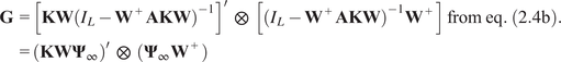 $$ {\displaystyle \begin{array}{c}\mathbf{G}={\left[\mathbf{KW}{\left({I}_L-{\mathbf{W}}^{+}\mathbf{AKW}\right)}^{-1}\right]}^{\prime}\hskip0.5em \otimes \hskip0.5em \left[{\left({I}_L-{\mathbf{W}}^{+}\mathbf{AKW}\right)}^{-1}{\mathbf{W}}^{+}\right]\hskip0.24em \mathrm{from}\hskip0.32em \mathrm{eq}.\hskip0.32em \left(2.4\mathrm{b}\right).\\ {}={\left(\mathbf{KW}{\boldsymbol{\Psi}}_{\infty}\right)}^{\prime}\hskip0.5em \otimes \hskip0.5em \left({\boldsymbol{\Psi}}_{\infty }{\mathbf{W}}^{+}\right)\end{array}} $$ $ \square $
Proof. We apply Proposition A.1 to the function $ g:\beta \to vec\left({\boldsymbol{\Psi}}_{\infty}\right) $
.
$ g:\beta \to vec\left({\boldsymbol{\Psi}}_{\infty}\right) $
.
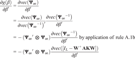 $$ {\displaystyle \begin{array}{c}\frac{\partial g\left(\beta \right)}{\partial {\beta}^{\prime }}=\frac{\partial vec\left({\boldsymbol{\Psi}}_{\infty}\right)}{\partial {\beta}^{\prime }}\\ {}=\frac{\partial vec\left({\boldsymbol{\Psi}}_{\infty}\right)}{\partial vec{\left({{\boldsymbol{\Psi}}_{\infty}}^{-1}\right)}^{\prime }}\frac{\partial vec\left({{\boldsymbol{\Psi}}_{\infty}}^{-1}\right)}{\partial {\beta}^{\prime }}\\ {}=-\left({{\boldsymbol{\Psi}}_{\infty}}^{\prime}\hskip0.5em \otimes \hskip0.5em {\boldsymbol{\Psi}}_{\infty}\right)\frac{\partial vec\left({{\boldsymbol{\Psi}}_{\infty}}^{-1}\right)}{\partial {\beta}^{\prime }}\hskip0.4em \mathrm{by}\hskip0.32em \mathrm{application}\ \mathrm{of}\ \mathrm{rule}\hskip0.4em \mathrm{A}.1\mathrm{b}\\ {}=-\left({{\boldsymbol{\Psi}}_{\infty}}^{\prime}\hskip0.5em \otimes \hskip0.5em {\boldsymbol{\Psi}}_{\infty}\right)\frac{\partial vec\left(\left[{I}_L-{\mathbf{W}}^{+}\mathbf{AKW}\right]\right)}{\partial {\beta}^{\prime }}\end{array}} $$
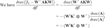 $$ {\displaystyle \begin{array}{c}\mathrm{We}\ \mathrm{have}\hskip0.4em \frac{\partial vec\left(\left[{I}_L-{\mathbf{W}}^{+}\mathbf{AKW}\right]\right)}{\partial {\beta}^{\prime }}=-\frac{\partial vec\left({\mathbf{W}}^{+}\mathbf{AKW}\right)}{\partial {\beta}^{\prime }}\\ {}=-\left({\mathbf{W}}^{\prime }{\mathbf{K}}^{\prime}\hskip0.5em \otimes \hskip0.5em {\mathbf{W}}^{+}\right)\frac{\partial vec\left(\mathbf{A}\right)}{\partial vec{\left(\mathbf{A}\right)}^{\prime }}\\ {}=-\left({\mathbf{W}}^{\prime }{\mathbf{K}}^{\prime}\hskip0.5em \otimes \hskip0.5em {\mathbf{W}}^{+}\right)\end{array}} $$
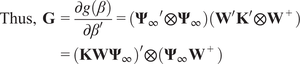 $$ {\displaystyle \begin{array}{c}\mathrm{Thus},\hskip0.4em \mathbf{G}=\frac{\partial g\left(\beta \right)}{\partial {\beta}^{\prime }}=\left({{\boldsymbol{\Psi}}_{\infty}}^{\prime}\otimes {\boldsymbol{\Psi}}_{\infty}\right)\left({\mathbf{W}}^{\prime }{\mathbf{K}}^{\prime}\otimes {\mathbf{W}}^{+}\right)\\ {}={\left(\mathbf{KW}{\boldsymbol{\Psi}}_{\infty}\right)}^{\prime}\otimes \left({\boldsymbol{\Psi}}_{\infty }{\mathbf{W}}^{+}\right)\end{array}} $$
Proposition A.4. (Asymptotic distribution of $ \hat{\alpha} $
).
$ \hat{\alpha} $
).
We remind that we derived two explicit formulas of $ \alpha $
given in Equations (2.3b) and (2.3c), and we recall that
$ \alpha $
given in Equations (2.3b) and (2.3c), and we recall that $ \alpha =\overline{{\boldsymbol{\Psi}}_{\infty}\mathbf{b}} $
.
$ \alpha =\overline{{\boldsymbol{\Psi}}_{\infty}\mathbf{b}} $
.
We note $ \hat{\beta}= vec\left(\hat{\mathbf{A}}\right) $
and
$ \hat{\beta}= vec\left(\hat{\mathbf{A}}\right) $
and $ \beta = vec\left(\mathbf{A}\right) $
.
$ \beta = vec\left(\mathbf{A}\right) $
.
If
 $$ \sqrt{T}\left(\hat{\beta}-\beta \right)\overset{d}{\to}\mathcal{N}\left(0,{\boldsymbol{\Sigma}}_{\hat{\beta}}\right) $$
Then
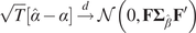 $$ \sqrt{T}\left[\hat{\alpha}-\alpha \right]\overset{d}{\to}\mathcal{N}\left(0,\mathbf{F}{\boldsymbol{\Sigma}}_{\hat{\beta}}{\mathbf{F}}^{\prime}\right) $$
with
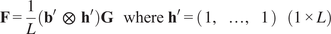 $$ \mathbf{F}=\frac{1}{L}\left({\mathbf{b}}^{\prime}\hskip0.5em \otimes \hskip0.5em {\mathbf{h}}^{\prime}\right)\mathbf{G}\hskip1em \mathrm{where}\hskip0.4em {\mathbf{h}}^{\prime }=\left(\begin{array}{ccc}1,& \dots, & 1\end{array}\right)\hskip1em \left(1\times L\right) $$ $ \square $
Proof. Using Proposition A.3, we have
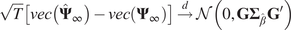 $$ \sqrt{T}\left[ vec\left({\hat{\boldsymbol{\Psi}}}_{\infty}\right)- vec\left({\boldsymbol{\Psi}}_{\infty}\right)\right]\overset{d}{\to}\mathcal{N}\left(0,\mathbf{G}{\boldsymbol{\Sigma}}_{\hat{\beta}}{\mathbf{G}}^{\prime}\right) $$
Next, we apply Proposition A.1 to the function $ g: vec\left({\boldsymbol{\Psi}}_{\infty}\right)\to \overline{{\boldsymbol{\Psi}}_{\infty}\mathbf{b}} $
. We notice that
$ g: vec\left({\boldsymbol{\Psi}}_{\infty}\right)\to \overline{{\boldsymbol{\Psi}}_{\infty}\mathbf{b}} $
. We notice that $ \overline{{\boldsymbol{\Psi}}_{\infty}\mathbf{b}}=\frac{1}{L}{\mathbf{h}}^{\prime}\;{\boldsymbol{\Psi}}_{\infty}\mathbf{b} $
.
$ \overline{{\boldsymbol{\Psi}}_{\infty}\mathbf{b}}=\frac{1}{L}{\mathbf{h}}^{\prime}\;{\boldsymbol{\Psi}}_{\infty}\mathbf{b} $
.
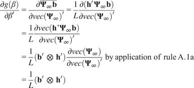 $$ {\displaystyle \begin{array}{c}\frac{\partial g\left(\beta \right)}{\partial {\beta}^{\prime }}=\frac{\partial \overline{{\boldsymbol{\Psi}}_{\infty}\mathbf{b}}}{\partial vec{\left({\boldsymbol{\Psi}}_{\infty}\right)}^{\prime }}=\frac{1}{L}\frac{\partial \left({\mathbf{h}}^{\prime}\;{\boldsymbol{\Psi}}_{\infty}\mathbf{b}\right)}{\partial vec{\left({\boldsymbol{\Psi}}_{\infty}\right)}^{\prime }}\\ {}=\frac{1}{L}\frac{\partial vec\left(\mathbf{h}'{\boldsymbol{\Psi}}_{\infty}\mathbf{b}\right)}{\partial vec{\left({\boldsymbol{\Psi}}_{\infty}\right)}^{\prime }}\\ {}=\frac{1}{L}\left({\mathbf{b}}^{\prime}\hskip0.5em \otimes \hskip0.5em {\mathbf{h}}^{\prime}\right)\frac{\partial vec\left({\boldsymbol{\Psi}}_{\infty}\right)}{\partial vec{\left({\boldsymbol{\Psi}}_{\infty}\right)}^{\prime }}\hskip0.4em \mathrm{by}\hskip0.3em \mathrm{application}\ \mathrm{of}\ \mathrm{rule}\hskip0.3em \mathrm{A}.1\mathrm{a}\\ {}=\frac{1}{L}\left({\mathbf{b}}^{\prime}\hskip0.5em \otimes \hskip0.5em {\mathbf{h}}^{\prime}\right)\end{array}} $$
Thus,
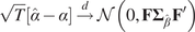 $$ \sqrt{T}\left[\hat{\alpha}-\alpha \right]\overset{d}{\to}\mathcal{N}\left(0,\mathbf{F}{\boldsymbol{\Sigma}}_{\hat{\beta}}{\mathbf{F}}^{\prime}\right) $$
with
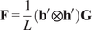 $$ \mathbf{F}=\frac{1}{L}\left({\mathbf{b}}^{\prime}\otimes {\mathbf{h}}^{\prime}\right)\mathbf{G} $$
■
A.4. Bootstrap-based CI
CIs can be obtained by bootstrapping of the residuals. In this study, we used four variations of bootstrapping methods:
-
• Bootstrapping with resampling of the residuals (Efron and Tibshirani, Reference Efron and Tibshirani1995) and standard percentile interval
-
• Bootstrapping with resampling of the residuals and with Hall’s percentile interval (Hall, Reference Hall1992)
-
• Bootstrapping with sampling from the covariance of the residuals (Efron and Tibshirani, Reference Efron and Tibshirani1995) and standard percentile interval.
-
• Bootstrapping with sampling from the covariance of the residuals and with Hall’s percentile interval (Hall, Reference Hall1992)
For all these methods, the first step is to sample new residuals from the original fitted model. The methods differ in their way of sampling new residuals:
-
• For the methods with resampling of the residuals, a sample of size
$ T $
is drawn with replacement from the residuals. The sampled residuals are then centered. -
• For the methods with sampling from the covariance, T samples are generated from the estimated covariance matrix of the residuals.

For all the methods, new data are created using the original model but by adding the sampled residuals instead of the original residuals. The model is then reestimated, giving new model parameters. From there, the quantity of interest (e.g., the sensitivity, or the LREs) is estimated for the current bootstrap realization and stored for later use. All these steps are repeated for the number of chosen bootstrap realizations. For normal bootstrapping, the CI is computed directly as the percentile of the quantity of interest across all the bootstrap realizations. In contrast, for Hall’s percentile interval bootstrapping, the CIs are corrected following the procedure given by Hall (Reference Hall1992).
B. Additional results
B.1. Experiment 1: Benchmark of methods for the LREs
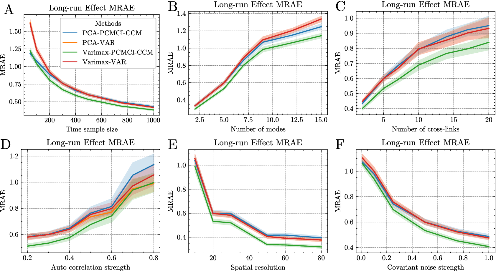
Figure B1. Comparison of four methods to estimate the long-run effects mentioned in Section 3.1.1. The different subfigures represent the change of the evaluation metrics (y-axis) for the different methods evaluated as a function of the (A) number of time samples available, (B) number of modes, (C) number of links between the modes, (D) strength of the autocorrelation of each mode, (E) resolution of the spatial grid, and (F) strength of the covariant noise. The evaluation metric is the relative absolute error (RAE) between the ground truth and estimated long-run effects. The mean RAE (MRAE) is represented by the solid lines, and the shaded areas depict the 90% range of the MRAE metric across the 250 realizations.
B.2. Experiment 2: CIs comparison
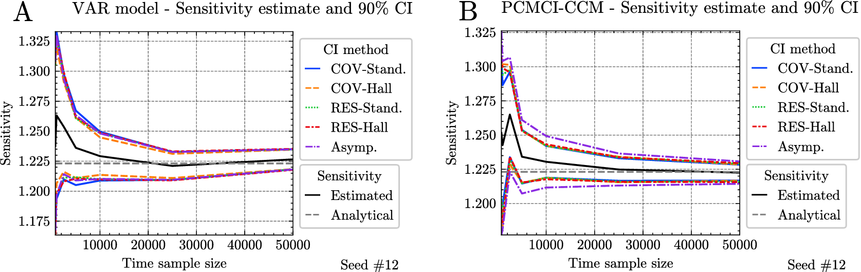
Figure B2. Same as Figure 6 but with a different seed (here seed 12). Comparison of the confidence interval methods mentioned in Section 3.1.2 to build a 90% confidence interval of the sensitivity ( $ y $
-axis) for varying time sample size (
$ y $
-axis) for varying time sample size ( $ x $
-axis) for one particular realization of an SAVAR model (seed 12). We estimate the linear coefficient matrix with a VAR model (A) or with PCMCI–CCM (B).
$ x $
-axis) for one particular realization of an SAVAR model (seed 12). We estimate the linear coefficient matrix with a VAR model (A) or with PCMCI–CCM (B).


 Open access