


1 Introduction
Let X be a compact Hausdorff space and
 $ \sigma : X \to X $
a local homeomorphism of
$ \sigma : X \to X $
a local homeomorphism of
 $ X $
onto itself. The so-called Deaconu–Renault groupoid and its associated
$ X $
onto itself. The so-called Deaconu–Renault groupoid and its associated
 $C^*$
-algebra corresponding to the pair
$C^*$
-algebra corresponding to the pair
 $ ({X,\sigma }) $
were first studied by Deaconu in [Reference Deaconu7] based on a construction of Renault in [Reference Renault22] in the setting of groupoids of Cuntz algebras. Deaconu adapted Renault’s construction by replacing the shift map on the infinite sequence space with a local homeomorphism. Renault further generalized this construction to local homeomorphisms defined on open subsets in [Reference Renault23]. The étale groupoid associated to a finite family of commuting local homeomorphisms of a compact metric space has gone by various names including Deaconu–Renault groupoids of higher rank and the semidirect product groupoid corresponding to the action of the semigroup
$ ({X,\sigma }) $
were first studied by Deaconu in [Reference Deaconu7] based on a construction of Renault in [Reference Renault22] in the setting of groupoids of Cuntz algebras. Deaconu adapted Renault’s construction by replacing the shift map on the infinite sequence space with a local homeomorphism. Renault further generalized this construction to local homeomorphisms defined on open subsets in [Reference Renault23]. The étale groupoid associated to a finite family of commuting local homeomorphisms of a compact metric space has gone by various names including Deaconu–Renault groupoids of higher rank and the semidirect product groupoid corresponding to the action of the semigroup
 $ \mathbb {N}^{k} $
[Reference Exel and Renault10]. In [Reference Renault and Williams26], these groupoids were generalized to the setting of partial semigroup actions. Our main purpose in this paper is the study of these groupoids, their associated
$ \mathbb {N}^{k} $
[Reference Exel and Renault10]. In [Reference Renault and Williams26], these groupoids were generalized to the setting of partial semigroup actions. Our main purpose in this paper is the study of these groupoids, their associated
 $ C^{\ast } $
-algebras, and KMS states which arise naturally on a specific class of related dynamical systems. This is a sufficiently broad class to include higher-rank graph
$ C^{\ast } $
-algebras, and KMS states which arise naturally on a specific class of related dynamical systems. This is a sufficiently broad class to include higher-rank graph
 $C^*$
-algebras associated to finite k-graphs. We develop cohomological methods to characterize
$C^*$
-algebras associated to finite k-graphs. We develop cohomological methods to characterize
 $ 1 $
-cocycles on these
$ 1 $
-cocycles on these
 $ C^{\ast } $
-algebras, which in turn give rise to one-parameter automorphism groups. This leads us to study the KMS states on these
$ C^{\ast } $
-algebras, which in turn give rise to one-parameter automorphism groups. This leads us to study the KMS states on these
 $ C^{\ast } $
-algebras.
$ C^{\ast } $
-algebras.
KMS states have their origin in equilibrium statistical mechanics and have long been a very fruitful tool in the study of operator algebras. For the precise definition of KMS states see [Reference Farsi, Gillaspy, Larsen and Packer12] and the references contained therein. In this paper, we study KMS states for groupoids associated to a finite family of commuting local homeomorphisms of a compact metric space by further developing a Ruelle–Perron–Frobenius (RPF) theory of dynamical systems of several commuting operators. Although an RPF theory for free abelian semigroups has been introduced by Carvalho, Rodrigues, and Varandas in [Reference Carvalho, Rodrigues and Varandas4, Reference Carvalho, Rodrigues and Varandas5], their main emphasis was on skew products, random walks, and topological entropy, whereas our emphasis here will be on the connection to the
 $ C^{\ast } $
-algebras and the use of the Ruelle–Perron–Frobenius operator to prove the existence of measures with appropriate properties (hence states with related properties).
$ C^{\ast } $
-algebras and the use of the Ruelle–Perron–Frobenius operator to prove the existence of measures with appropriate properties (hence states with related properties).
In the groupoid perspective, as first explained by Renault in [Reference Renault22], time evolutions (dynamics) on the reduced
 $ C^{\ast } $
-algebra of a groupoid
$ C^{\ast } $
-algebra of a groupoid
 $ \mathcal {G} $
are implemented by continuous real-valued
$ \mathcal {G} $
are implemented by continuous real-valued
 $ 1 $
-cocycles on
$ 1 $
-cocycles on
 $ \mathcal {G} $
and the task of understanding the KMS states for these dynamics on
$ \mathcal {G} $
and the task of understanding the KMS states for these dynamics on
 $ C^{\ast }_{\textrm {r}} ({\mathcal {G}}) $
requires, at a minimum, identifying the measures on the unit space of
$ C^{\ast }_{\textrm {r}} ({\mathcal {G}}) $
requires, at a minimum, identifying the measures on the unit space of
 $ \mathcal {G} $
that are quasi-invariant. There are now refinements of Renault’s result; see, for example, work by Neshveyev [Reference Neshveyev20] and Thomsen [Reference Thomsen30]. More recently, Christensen’s paper [Reference Christensen6] combines quasi-invariant measures with a certain group of symmetries to describe KMS states on groupoid
$ \mathcal {G} $
that are quasi-invariant. There are now refinements of Renault’s result; see, for example, work by Neshveyev [Reference Neshveyev20] and Thomsen [Reference Thomsen30]. More recently, Christensen’s paper [Reference Christensen6] combines quasi-invariant measures with a certain group of symmetries to describe KMS states on groupoid
 $ C^{\ast } $
-algebras for locally compact second countable Hausdorff étale groupoids.
$ C^{\ast } $
-algebras for locally compact second countable Hausdorff étale groupoids.
Our analysis of the KMS states on groupoids associated to a finite family of commuting local homeomorphisms of a compact metric space stems from a new characterization of their continuous real-valued
 $1$
-cocycles, which in a nutshell are determined completely by a
$1$
-cocycles, which in a nutshell are determined completely by a
 $ k $
-tuple of continuous real-valued functions on the unit space of the groupoid satisfying canonical identities. In so doing, we give an isomorphism between the first monoid cohomology of
$ k $
-tuple of continuous real-valued functions on the unit space of the groupoid satisfying canonical identities. In so doing, we give an isomorphism between the first monoid cohomology of
 $ \mathbb {N}^{k} $
with coefficients in the module
$ \mathbb {N}^{k} $
with coefficients in the module
 $ \operatorname {C} ({X,H}) $
of continuous functions on X with values in H, where
$ \operatorname {C} ({X,H}) $
of continuous functions on X with values in H, where
 $ H $
is a locally compact abelian group, and the first continuous cocycle groupoid cohomology taking values in
$ H $
is a locally compact abelian group, and the first continuous cocycle groupoid cohomology taking values in
 $ H $
.
$ H $
.
We base our constructions on the established analysis of KMS states on Deaconu–Renault groupoids of [Reference Exel9, Reference Ionescu and Kumjian13, Reference Kumjian and Renault17, Reference Renault24], together with an extended Ruelle–Perron–Frobenius theory for dynamical systems of several commuting operators, modelled on the one-dimensional theory of Ruelle [Reference Ruelle27] and Walters [Reference Walters31].
In [Reference Kumjian and Renault17], Kumjian and Renault associated KMS states to Ruelle operators constructed on a groupoid arising from a single expansive map and, in [Reference Ionescu and Kumjian13], Ionescu and Kumjian related the associated states to Hausdorff measures, which led to applications to KMS states on Cuntz algebras,
 $ C^{\ast } $
-algebras arising from directed graphs, and
$ C^{\ast } $
-algebras arising from directed graphs, and
 $ C^{\ast } $
-algebras associated to fractafolds. In addition, Ruelle operators were used in [Reference Bissacot, Exel, Frausino and Raszeja2]. In this paper, we generalize some of these results to groupoids associated to a finite family of commuting local homeomorphisms of a compact metric space. In particular, we deduce that in order for the adjoint of the Ruelle operator associated to a finite family of commuting local homeomorphism to have an eigenmeasure, it is necessary and sufficient that the adjoint of the Ruelle operator corresponding to a non-trivial product of the local homeomorphisms have that same eigenmeasure, thus reducing matters to the one-dimensional case studied by Walters.
$ C^{\ast } $
-algebras associated to fractafolds. In addition, Ruelle operators were used in [Reference Bissacot, Exel, Frausino and Raszeja2]. In this paper, we generalize some of these results to groupoids associated to a finite family of commuting local homeomorphisms of a compact metric space. In particular, we deduce that in order for the adjoint of the Ruelle operator associated to a finite family of commuting local homeomorphism to have an eigenmeasure, it is necessary and sufficient that the adjoint of the Ruelle operator corresponding to a non-trivial product of the local homeomorphisms have that same eigenmeasure, thus reducing matters to the one-dimensional case studied by Walters.
Ruelle operators are important tools in mathematical physics, particularly thermodynamics, and yield a formulation of a ‘continuous’ extension of the seminal Perron–Frobenius theorem. Ruelle’s classical result, known as the ‘Ruelle–Perron–Frobenius (RPF) theorem’, gives a sufficient condition for a Ruelle triple to satisfy the unique positive eigenvalue condition [Reference Ruelle27, Reference Ruelle28]. In [Reference Walters32], building on earlier work of Bowen, Walters gave criteria for the RPF theorem to hold for more general Ruelle triples
 $ ({X,\sigma ,\varphi }) $
merely demanding that
$ ({X,\sigma ,\varphi }) $
merely demanding that
 $ X $
be a metric space,
$ X $
be a metric space,
 $ \sigma $
be positively expansive and exact, and
$ \sigma $
be positively expansive and exact, and
 $ \varphi $
satisfy a smoothness condition. We extend the RPF theorem to certain Ruelle triples of type
$ \varphi $
satisfy a smoothness condition. We extend the RPF theorem to certain Ruelle triples of type
 $ ({X,\sigma ,\varphi }) := ({X,\sigma _{i},\varphi _{i}})_{i = 1}^{k} $
, where the
$ ({X,\sigma ,\varphi }) := ({X,\sigma _{i},\varphi _{i}})_{i = 1}^{k} $
, where the
 $ \sigma _{i} $
form a commuting family of local homeomorphisms which are positively expansive and exact, and the
$ \sigma _{i} $
form a commuting family of local homeomorphisms which are positively expansive and exact, and the
 $ \varphi _{i} $
satisfy the Walters conditions.
$ \varphi _{i} $
satisfy the Walters conditions.
To derive our generalization of the the RPF theorem, we first need to construct continuous
 $ 1 $
-cocycles on the groupoid
$ 1 $
-cocycles on the groupoid
 $ \mathcal {G} ({X,\sigma }) $
arising from a
$ \mathcal {G} ({X,\sigma }) $
arising from a
 $ k $
-tuple of commuting local homeomorphisms on
$ k $
-tuple of commuting local homeomorphisms on
 $ X $
with values in
$ X $
with values in
 $ \mathbb {R} $
. In order to study this in the greatest possible generality, we first study the problem of calculating
$ \mathbb {R} $
. In order to study this in the greatest possible generality, we first study the problem of calculating
 $ H^{1} ({\mathbb {N}^{k},A}) $
, where
$ H^{1} ({\mathbb {N}^{k},A}) $
, where
 $ A $
is an
$ A $
is an
 $ \mathbb {N}^{k} $
-module. In Theorem 3.4, we are able to give an explicit formula for all elements of
$ \mathbb {N}^{k} $
-module. In Theorem 3.4, we are able to give an explicit formula for all elements of
 $ Z^{1} ({\mathbb {N}^{k},A}) $
from
$ Z^{1} ({\mathbb {N}^{k},A}) $
from
 $ k $
-tuples in
$ k $
-tuples in
 $ A^{k} $
satisfying what we call the ‘module cocycle condition’ and describe which of these are coboundaries. In the case
$ A^{k} $
satisfying what we call the ‘module cocycle condition’ and describe which of these are coboundaries. In the case
 $ k = 1 $
, this formula is similar to the formula given in [Reference Deaconu, Kumjian and Muhly8].
$ k = 1 $
, this formula is similar to the formula given in [Reference Deaconu, Kumjian and Muhly8].
We apply this theorem by starting with a
 $ k $
-tuple of commuting local homeomorphisms of
$ k $
-tuple of commuting local homeomorphisms of
 $ X $
and using them to give
$ X $
and using them to give
 $ \operatorname {C} ({X,H}) $
an
$ \operatorname {C} ({X,H}) $
an
 $ \mathbb {N}^{k} $
-module structure for any locally compact abelian group
$ \mathbb {N}^{k} $
-module structure for any locally compact abelian group
 $ H $
. We then provide an explicit isomorphism between
$ H $
. We then provide an explicit isomorphism between
 $ H^{1} ({\mathbb {N}^{k},\operatorname {C} ({X,H})}) $
and the first cohomology group
$ H^{1} ({\mathbb {N}^{k},\operatorname {C} ({X,H})}) $
and the first cohomology group
 $ H_{\operatorname {cont}}^{1} ({\mathcal {G} ({X,\sigma }),H}) $
of the groupoid
$ H_{\operatorname {cont}}^{1} ({\mathcal {G} ({X,\sigma }),H}) $
of the groupoid
 $ \mathcal {G} ({X,\sigma }) $
. Specializing to the case where
$ \mathcal {G} ({X,\sigma }) $
. Specializing to the case where
 $ H = \mathbb {R} $
, we obtain explicit formulas for elements of
$ H = \mathbb {R} $
, we obtain explicit formulas for elements of
 $ Z_{\operatorname {cont}}^{1} ({\mathcal {G} ({X,\sigma }),\mathbb {R}}) $
that we use in the generalized RPF theorem.
$ Z_{\operatorname {cont}}^{1} ({\mathcal {G} ({X,\sigma }),\mathbb {R}}) $
that we use in the generalized RPF theorem.
Recently there has been great interest (cf. [Reference an Huef, Laca, Raeburn and Sims1, Reference Farsi, Gillaspy, Larsen and Packer12, Reference McNamara18]) in the KMS states associated to one-parameter dynamical systems on
 $ C^{\ast } ({\Lambda }) $
, where
$ C^{\ast } ({\Lambda }) $
, where
 $ \Lambda $
is a higher-rank graph and the dynamics arises either from the canonical gauge action of
$ \Lambda $
is a higher-rank graph and the dynamics arises either from the canonical gauge action of
 $ \mathbb {T}^{k} $
on
$ \mathbb {T}^{k} $
on
 $ C^{\ast } ({\Lambda }) $
or from a generalized gauge action. In particular, for a finite strongly connected
$ C^{\ast } ({\Lambda }) $
or from a generalized gauge action. In particular, for a finite strongly connected
 $ k $
-graph, in [Reference an Huef, Laca, Raeburn and Sims1, Reference Farsi, Gillaspy, Larsen and Packer12, Reference McNamara18], one can endow
$ k $
-graph, in [Reference an Huef, Laca, Raeburn and Sims1, Reference Farsi, Gillaspy, Larsen and Packer12, Reference McNamara18], one can endow
 $ C^{\ast } ({\Lambda }) $
with a (generalized) gauge dynamics and show the existence of unique KMS states. Here, we are able to recover some of the results in [Reference an Huef, Laca, Raeburn and Sims1, Reference Farsi, Gillaspy, Larsen and Packer12, Reference McNamara18] from a different perspective, using the Ruelle–Perron–Frobenius theorem and the generalized gauge dynamics that we obtain from our description of
$ C^{\ast } ({\Lambda }) $
with a (generalized) gauge dynamics and show the existence of unique KMS states. Here, we are able to recover some of the results in [Reference an Huef, Laca, Raeburn and Sims1, Reference Farsi, Gillaspy, Larsen and Packer12, Reference McNamara18] from a different perspective, using the Ruelle–Perron–Frobenius theorem and the generalized gauge dynamics that we obtain from our description of
 $ Z_{\operatorname {cont}}^{1} ({\mathcal {G} ({X,\sigma }),\mathbb {R}}) $
given in Proposition 3.10.
$ Z_{\operatorname {cont}}^{1} ({\mathcal {G} ({X,\sigma }),\mathbb {R}}) $
given in Proposition 3.10.
We now outline the structure of the paper. Section 2 introduces classical Ruelle triples, triples that satisfy the unique positive eigenvalue condition (see Definition 2.3), and Ruelle operators. These are basic objects that we will generalize to higher dimensions in §4. We also review several essential results of Walters, Bowen, and Ruelle in this section. In §3, we review the construction of the groupoid
 $\mathcal {G} ({X,\sigma })$
associated to a finite family
$\mathcal {G} ({X,\sigma })$
associated to a finite family
 $\sigma $
of commuting local homeomorphisms of a compact metric space X, and then briefly review level-one semigroup cohomology and continuous groupoid cohomology and relate the two. We also give an algebraic way of constructing all continuous
$\sigma $
of commuting local homeomorphisms of a compact metric space X, and then briefly review level-one semigroup cohomology and continuous groupoid cohomology and relate the two. We also give an algebraic way of constructing all continuous
 $ 1 $
-cocycles in both the semigroup and groupoid cases. Our main interest are continuous real-valued
$ 1 $
-cocycles in both the semigroup and groupoid cases. Our main interest are continuous real-valued
 $ 1 $
-cocycles on
$ 1 $
-cocycles on
 $ \mathcal {G} ({X,\sigma }) $
. In §4, we introduce
$ \mathcal {G} ({X,\sigma }) $
. In §4, we introduce
 $ k $
-Ruelle dynamical systems, the related families of commuting Ruelle operators and their duals, and their eigenmeasures. In §5, we use the results of the previous sections to consider the Radon–Nikodym problem for these groupoids, which provides a link between quasi-invariant measures for the groupoids
$ k $
-Ruelle dynamical systems, the related families of commuting Ruelle operators and their duals, and their eigenmeasures. In §5, we use the results of the previous sections to consider the Radon–Nikodym problem for these groupoids, which provides a link between quasi-invariant measures for the groupoids
 $\mathcal {G} ({X,\sigma })$
and KMS states for a generalized gauge dynamics. In particular, we prove that if the generalized Ruelle operator associated to a k-Ruelle system has an eigenmeasure with eigenvalue one, then there exists a KMS state for the generalized gauge dynamics coming from certain groupoid
$\mathcal {G} ({X,\sigma })$
and KMS states for a generalized gauge dynamics. In particular, we prove that if the generalized Ruelle operator associated to a k-Ruelle system has an eigenmeasure with eigenvalue one, then there exists a KMS state for the generalized gauge dynamics coming from certain groupoid
 $ 1 $
-cocycles related to the groupoid
$ 1 $
-cocycles related to the groupoid
 $ C^{\ast } $
-algebra. Finally, in §6, we apply the results obtained thus far to answer some existence and uniqueness questions concerning KMS states for a generalized gauge dynamics associated to higher-rank graphs.
$ C^{\ast } $
-algebra. Finally, in §6, we apply the results obtained thus far to answer some existence and uniqueness questions concerning KMS states for a generalized gauge dynamics associated to higher-rank graphs.
1.1 Notation and conventions
In the rest of the paper, we will use the following notational conventions. We denote by
 $ \mathbb {N} $
the semigroup of natural integers
$ \mathbb {N} $
the semigroup of natural integers
 $ \{ 0,1,2,\ldots \} $
and by
$ \{ 0,1,2,\ldots \} $
and by
 $ \mathbb {N}_{>0} $
the set of positive elements of
$ \mathbb {N}_{>0} $
the set of positive elements of
 $\mathbb {N}$
. For fixed
$\mathbb {N}$
. For fixed
 $ k \in \mathbb {N}_{>0} $
, we denote by
$ k \in \mathbb {N}_{>0} $
, we denote by
 $\mathbb {N}^k$
the semigroup of all ordered k-tuples of elements of
$\mathbb {N}^k$
the semigroup of all ordered k-tuples of elements of
 $\mathbb {N}$
and by
$\mathbb {N}$
and by
 $ [ k ] $
the set
$ [ k ] $
the set
 $[ k ]=\{ 1,\ldots ,k \} $
. We define the length
$[ k ]=\{ 1,\ldots ,k \} $
. We define the length
 $\lvert n \rvert $
of an element
$\lvert n \rvert $
of an element
 $n=(n_1,\ldots, n_k) \in \mathbb {N}^k$
by
$n=(n_1,\ldots, n_k) \in \mathbb {N}^k$
by
 $\lvert n \rvert := n_{1} + \cdots + n_{k} $
.
$\lvert n \rvert := n_{1} + \cdots + n_{k} $
.
For every compact Hausdorff space
 $ X $
, and topological locally compact group H, we let
$ X $
, and topological locally compact group H, we let
 $ C(X,H) $
be the group of continuous functions from X to H. In many instances
$ C(X,H) $
be the group of continuous functions from X to H. In many instances
 $H=\mathbb {R} $
in this paper. We will also let
$H=\mathbb {R} $
in this paper. We will also let
 $ \mathcal {M} ({X}) $
denote the Banach space of finite signed Borel measures on the Borel subsets of
$ \mathcal {M} ({X}) $
denote the Banach space of finite signed Borel measures on the Borel subsets of
 $ X $
, which is isometrically isomorphic to the dual space
$ X $
, which is isometrically isomorphic to the dual space
 $ C(X,\mathbb {R})' $
of
$ C(X,\mathbb {R})' $
of
 $ C(X,\mathbb {R}) $
.Footnote †
$ C(X,\mathbb {R}) $
.Footnote †
For every (locally) compact Hausdorff étale groupoid
 $ \mathcal {G} $
, there is a standard dense linear embedding of
$ \mathcal {G} $
, there is a standard dense linear embedding of
 $ \operatorname {C_{c}} ({\mathcal {G}}) $
into
$ \operatorname {C_{c}} ({\mathcal {G}}) $
into
 $ C^{\ast }_{\textrm {r}} ({\mathcal {G}}) $
. The groupoids that we study are amenable, so, unless there is a danger of confusion, we shall identify
$ C^{\ast }_{\textrm {r}} ({\mathcal {G}}) $
. The groupoids that we study are amenable, so, unless there is a danger of confusion, we shall identify
 $ f \in \operatorname {C_{c}} ({\mathcal {G}}) $
with its image (also denoted by
$ f \in \operatorname {C_{c}} ({\mathcal {G}}) $
with its image (also denoted by
 $ f $
) in
$ f $
) in
 $ C^{\ast }_{\textrm {r}} ({\mathcal {G}}) \cong C^{\ast } ({\mathcal {G}}) $
.
$ C^{\ast }_{\textrm {r}} ({\mathcal {G}}) \cong C^{\ast } ({\mathcal {G}}) $
.
In what follows,
 $ X $
will always denote a (non-empty) compact Hausdorff topological space.
$ X $
will always denote a (non-empty) compact Hausdorff topological space.
2 Ruelle triples and Ruelle operators
We begin by defining Ruelle triples and Ruelle operators (sometimes called transfer operators), which were introduced in [Reference Ruelle27] in the case of totally disconnected spaces and generalized to arbitrary compact metric spaces by Walters in [Reference Walters31, Reference Walters32]. These will be the basic objects of concern in this paper. Ruelle operators are important tools in mathematical physics, particularly thermodynamics, and yield a formulation of a ‘continuous’ extension of the classical Perron–Frobenius theorem. In [Reference Kumjian and Renault17], Kumjian and Renault associated KMS states to Ruelle operators constructed on a groupoid arising from a single expansive map on a compact metric space, which led to applications to KMS states on Cuntz
 $ C^{\ast } $
-algebras and
$ C^{\ast } $
-algebras and
 $ C^{\ast } $
-algebras associated to higher-rank graphs.
$ C^{\ast } $
-algebras associated to higher-rank graphs.
Definition 2.1. (Ruelle triples and operators)
-
(1) A Ruelle triple is an ordered triple
 $ ({X,T,\varphi }) ,$
where:
$ ({X,T,\varphi }) ,$
where:-
(a)
$ X $
is a compact metric space; -
(b)
$ T : X \to X $
is a surjective local homeomorphism; -
(c)
$ \varphi : X \to \mathbb {R} $
is a continuous function, that is,
$ \varphi \in \operatorname {C} ({X,\mathbb {R}}) $
.
-
-
(2) The Ruelle operator associated to a Ruelle triple
$ ({X,T,\varphi }) $
is the bounded linear operator defined by, for all
$$ \begin{align*}\mathcal{L}_{X,T,\varphi}: \operatorname{C} ({X,\mathbb{R}}) \to \operatorname{C} ({X,\mathbb{R}}) \end{align*} $$
$f \in \operatorname {C} ({X,\mathbb {R}}), ~ \text { for all } x \in X$
, (1)
$$ \begin{align} [ \mathcal{L}_{X,T,\varphi} ({f}) ] ({x}) := \sum_{y \in T^{- 1} [ \{ x \} ]} e^{\varphi ({y})} f ({y}). \end{align} $$


Our goal is to extend some results from [Reference Ionescu and Kumjian13, Reference Kumjian and Renault17, Reference Renault25] from a single local homeomorphism to commuting k-tuples of local homeomorphisms on
 $ X $
in part by employing cohomological methods. The following lemma follows from [Reference Exel and Renault10, Proposition 2.2].
$ X $
in part by employing cohomological methods. The following lemma follows from [Reference Exel and Renault10, Proposition 2.2].
Lemma 2.2. (Composition of Ruelle operators)
Let
 $ ({X,S,\varphi }) $
and
$ ({X,S,\varphi }) $
and
 $ ({X,T,\psi }) $
be Ruelle triples. Then
$ ({X,T,\psi }) $
be Ruelle triples. Then
 $ ({X,S \circ T,\varphi \circ T + \psi }) $
is a Ruelle triple and
$ ({X,S \circ T,\varphi \circ T + \psi }) $
is a Ruelle triple and
 $$ \begin{align*}\mathcal{L}_{X,S,\varphi} \circ \mathcal{L}_{X,T,\psi} = \mathcal{L}_{X,S \circ T,\varphi \circ h + \psi}. \end{align*} $$
We will now define an important subclass of Ruelle triples, those for which the positive eigenvalue problem for the dual Ruelle operator has a unique solution. These Ruelle triples enjoy important fixed-point properties and admit generalizations to dynamical systems that will be described in §4.
Definition 2.3. A Ruelle triple
 $ ({X,T,\varphi }) $
is said to satisfy the unique positive eigenvalue condition if there exists a unique ordered pair
$ ({X,T,\varphi }) $
is said to satisfy the unique positive eigenvalue condition if there exists a unique ordered pair
 $ ({\unicode{x3bb} ,\mu }) $
such that:
$ ({\unicode{x3bb} ,\mu }) $
such that:
-
(1)
$ \unicode{x3bb} $
is a positive real number; -
(2)
$ \mu $
is a Borel probability measure on
$ X $
; -
(3) if we denote by
$ ({\mathcal {L}_{X,T,\varphi }})^{\ast }: \mathcal {M} ({X}) \to \mathcal {M} ({X}) $
the dual of the Ruelle operator
$ \mathcal {L}_{X,T,\varphi } $
, then
$$ \begin{align*} ({\mathcal{L}_{X,T,\varphi}})^{\ast} ({\mu}) = \unicode{x3bb} \mu .\end{align*} $$


Ruelle’s classical result, known as the ‘Ruelle–Perron–Frobenius (RPF) theorem’, generalizes the seminal Perron–Frobenius theorem for primitive matrices to subshifts of finite type and gives a sufficient condition for a Ruelle triple to satisfy Definition 2.3 [Reference Ruelle27, Reference Ruelle28]. The RPF theorem below is taken from [Reference Exel9, Theorem 2.2].
To introduce the required notation to state the RPF theorem, fixing
 $ k \in \mathbb {N}_{> 0} $
, let
$ k \in \mathbb {N}_{> 0} $
, let
 $ A = ({A_{i,j}})_{i,j \in [ k ]}$
be an
$ A = ({A_{i,j}})_{i,j \in [ k ]}$
be an
 $ {n \times n} $
zero–one matrix with no row or column of zeros and let
$ {n \times n} $
zero–one matrix with no row or column of zeros and let
 $ ({\Sigma _{A},\sigma }) $
be the associated (one-sided) subshift of finite type, where
$ ({\Sigma _{A},\sigma }) $
be the associated (one-sided) subshift of finite type, where
 $ \Sigma _{A} $
is the compact topological subspace of the infinite product space
$ \Sigma _{A} $
is the compact topological subspace of the infinite product space
 $ \prod _{j \in \mathbb {N}} [ k ] $
defined by
$ \prod _{j \in \mathbb {N}} [ k ] $
defined by
 $$ \begin{align*}\Sigma_{A} := \bigg\{{x = ({x_{0},x_{1},x_{2},\ldots}) \in \prod_{j \in \mathbb{N}} [ k ]}~ \bigg|~{A_{x_{i},x_{i + 1}} = 1\quad\text{for all } i \geq 0}\bigg\} \end{align*} $$
and
 $ \sigma : \Sigma _{A} \to \Sigma _{A} $
is the ‘left shift’ given by
$ \sigma : \Sigma _{A} \to \Sigma _{A} $
is the ‘left shift’ given by
 $$ \begin{align*}\sigma ({x_{0},x_{1},x_{2},\ldots}) = ({x_{1},x_{2},x_{3},\ldots}). \end{align*} $$
Moreover, given a real number
 $ \beta \in ({0,1}) $
, we define a compatible metric
$ \beta \in ({0,1}) $
, we define a compatible metric
 $ d $
on
$ d $
on
 $ \Sigma _{A} $
by setting, for
$ \Sigma _{A} $
by setting, for
 $ x,y \in \Sigma _{A} $
and
$ x,y \in \Sigma _{A} $
and
 $ x \neq y $
,
$ x \neq y $
,
 $ d ({x,y}) = \beta ^{N ({x,y})} $
, where
$ d ({x,y}) = \beta ^{N ({x,y})} $
, where
 $ N ({x,y}) $
is the least integer
$ N ({x,y}) $
is the least integer
 $ N \in \mathbb {N} $
such that
$ N \in \mathbb {N} $
such that
 $ x_{i} \not = y_{i} $
. Furthermore,
$ x_{i} \not = y_{i} $
. Furthermore,
 $ \min ({\varnothing }) := \infty $
by convention; in this case
$ \min ({\varnothing }) := \infty $
by convention; in this case
 $d(x,y)=0$
.
$d(x,y)=0$
.
We can now state the Ruelle–Perron–Frobenius theorem as presented by Exel; see [Reference Exel9, Theorem 2.2] and [Reference Exel9, Proposition 2.3].
Theorem 2.4. (Ruelle–Perron–Frobenius theorem)
With notation as above, let
 $ \varphi $
be a continuous real-valued function defined on
$ \varphi $
be a continuous real-valued function defined on
 $ \Sigma _{A} $
. Suppose that:
$ \Sigma _{A} $
. Suppose that:
-
(1) there exists a positive integer
$ m $
such that
$ A^{m}> 0 $
(in the sense that all entries are positive); and -
(2)
$ \varphi $
is Hölder-continuous.


Then there exist a strictly positive function
 $ h \in \operatorname {C} ({\Sigma _{A},\mathbb {R}}) $
, a Borel probability measure
$ h \in \operatorname {C} ({\Sigma _{A},\mathbb {R}}) $
, a Borel probability measure
 $ \mu $
on
$ \mu $
on
 $ \Sigma _{A} $
, and a positive real number
$ \Sigma _{A} $
, and a positive real number
 $ \unicode{x3bb} $
such that:
$ \unicode{x3bb} $
such that:
-
(a)
$ ({\mathcal {L}_{\Sigma _A,\sigma ,\varphi }}) ({h}) = \unicode{x3bb} h $
; and -
(b)
$ ({\mathcal {L}_{\Sigma _A,\sigma ,\varphi }})^{\ast } ({\mu }) = \unicode{x3bb} \mu $
.
In particular,
 $ ({\Sigma _A,\sigma ,\varphi }) $
also satisfies the unique positive eigenvalue condition of Definition 2.3.
$ ({\Sigma _A,\sigma ,\varphi }) $
also satisfies the unique positive eigenvalue condition of Definition 2.3.
In the following, we will also refer to the Ruelle–Perron–Frobenius theorem as the RPF theorem. In [Reference Walters32, Reference Walters33], Walters gave criteria for the RPF theorem to hold for more general Ruelle triples
 $ ({X,T,\varphi }) $
, which was modified by Kumjian and Renault in [Reference Kumjian and Renault17], requiring that
$ ({X,T,\varphi }) $
, which was modified by Kumjian and Renault in [Reference Kumjian and Renault17], requiring that
 $ X $
be a metric space,
$ X $
be a metric space,
 $ T $
be positively expansive and exact, and
$ T $
be positively expansive and exact, and
 $ \varphi $
obey some summability condition. We will now detail these results.
$ \varphi $
obey some summability condition. We will now detail these results.
Definition 2.5. Let
 $ ({X,T,\varphi }) $
be a Ruelle triple and let
$ ({X,T,\varphi }) $
be a Ruelle triple and let
 $ d $
be the metric on
$ d $
be the metric on
 $ X $
. Consider the three conditions listed below.
$ X $
. Consider the three conditions listed below.
-
(1)
$ T $
is positively expansive, that is, there is an
$ \epsilon> 0 $
such that for all distinct
$ x,y \in X $
, there exists an
$ n \in \mathbb {N} $
such that
$ d ({T^{n} ({x}),T^{n} ({y})}) \geq \epsilon $
. -
(2)
$ T $
is exact, that is, for every non-empty open subset
$ U $
of
$ X $
, there exists an
$ n \in \mathbb {N} $
such that
$ T^{n} [ U ] = X $
. -
(3) There exist a compatible metric
$ d' $
on
$ X $
and positive numbers
$ \delta> 0 $
and
$ C> 0 $
with the property that for all
$n \in \mathbb {N}_{> 0} $
and for all
$ x,y \in X $
, we have that
$ d' ({T^{i} ({x}),{T}^{i} ({y})}) \leq \delta $
for all
$ i \in \{ 0,1,\ldots ,n - 1 \} $
implies that
$$ \begin{align*}\bigg\lvert{\sum_{i = 0}^{n - 1} \varphi ({T^{i} ({x})}) - \varphi ({T^{i} ({y})})}\bigg\rvert \leq C. \end{align*} $$


We say that
 $ (X, T,\varphi )$
satisfies the Walters conditions if it satisfies Conditions (1) and (2) above, and it satisfies the Bowen condition [Reference Bowen3] if it satisfies Condition (3) above. Moreover,
$ (X, T,\varphi )$
satisfies the Walters conditions if it satisfies Conditions (1) and (2) above, and it satisfies the Bowen condition [Reference Bowen3] if it satisfies Condition (3) above. Moreover,
 $ T $
is positively expansive if and only if there is an open neighbourhood
$ T $
is positively expansive if and only if there is an open neighbourhood
 $ U $
of
$ U $
of
 $ \Delta ({X}) $
, the diagonal of
$ \Delta ({X}) $
, the diagonal of
 $ X $
, such that for all distinct
$ X $
, such that for all distinct
 $ x,y \in X $
, there exists an
$ x,y \in X $
, there exists an
 $ n \in \mathbb {N} $
such that
$ n \in \mathbb {N} $
such that
 $ ({T^{n} ({x}),T^{n} ({y})}) \notin U $
.
$ ({T^{n} ({x}),T^{n} ({y})}) \notin U $
.
In all of our examples the function
 $\varphi $
is Hölder continuous, and that together with Condition (1) implies the Bowen condition, as noted in the following well-known proposition, whose proof is sketched in [Reference Kumjian and Renault17, p. 2071].
$\varphi $
is Hölder continuous, and that together with Condition (1) implies the Bowen condition, as noted in the following well-known proposition, whose proof is sketched in [Reference Kumjian and Renault17, p. 2071].
Proposition 2.6. Let
 $ ({X,T,\varphi }) $
be a Ruelle triple with T positively expansive. If
$ ({X,T,\varphi }) $
be a Ruelle triple with T positively expansive. If
 $ \varphi $
is Hölder-continuous with respect to a compatible metric
$ \varphi $
is Hölder-continuous with respect to a compatible metric
 $ d $
on
$ d $
on
 $ X $
, then Condition (3) of Definition 2.5 is satisfied for
$ X $
, then Condition (3) of Definition 2.5 is satisfied for
 $ d $
by
$ d $
by
 $ \varphi $
with respect to
$ \varphi $
with respect to
 $ T $
.
$ T $
.
The main results of [Reference Jiang and Ye14, Reference Walters32] yield the following theorem.
Theorem 2.7. A Ruelle triple satisfies the unique positive eigenvalue condition of Definition 2.3 if it satisfies the conditions in Definition 2.5.
In [Reference Jiang and Ye14], Jiang and Ye stated analogous conditions for weakly contractive iterated function systems for which results similar to Theorem 2.7 hold.
3 Continuous
$ 1 $
-cocycles on semigroups and continuous
$ 1 $
-cocycles on
$ \mathcal {G} ({X,\sigma }) $


3.1 Semigroup cocycles
We now discuss semigroup cocycles with values in a semigroup module
 $ A $
with the aim of explicitly constructing all
$ A $
with the aim of explicitly constructing all
 $ \mathbb {N}^{k} 1 $
-cocycles with values in the
$ \mathbb {N}^{k} 1 $
-cocycles with values in the
 $ \mathbb {N}^{k} $
-module
$ \mathbb {N}^{k} $
-module
 $ A $
.
$ A $
.
Definition 3.1. (Semigroup cocycles)
Let
 $ S $
be a semigroup and
$ S $
be a semigroup and
 $ A $
an
$ A $
an
 $ S $
-module, so that
$ S $
-module, so that
 $ A $
is an abelian group and there exists a homomorphism
$ A $
is an abelian group and there exists a homomorphism
 $ \pi : S \to \operatorname {End} ({A}) $
. When there is no danger of confusion, for
$ \pi : S \to \operatorname {End} ({A}) $
. When there is no danger of confusion, for
 $ s \in S $
and
$ s \in S $
and
 $ \alpha \in A $
, we denote by
$ \alpha \in A $
, we denote by
 $ s \alpha \in A $
the element
$ s \alpha \in A $
the element
 $ [ \pi ({s}) ] ({\alpha }) $
of
$ [ \pi ({s}) ] ({\alpha }) $
of
 $ A $
. Define
$ A $
. Define
 $ Z^{1} ({S,A}) $
to be the set of
$ Z^{1} ({S,A}) $
to be the set of
 $ A $
-valued
$ A $
-valued
 $ 1 $
-cocycles on
$ 1 $
-cocycles on
 $ S $
, that is,
$ S $
, that is,
 $ Z^{1} ({S,A}) $
is the set of functions
$ Z^{1} ({S,A}) $
is the set of functions
 $$ \begin{align*}Z^{1} ({S,A}) := \{ \gamma: S \to A ~ | ~ \gamma ({st}) = \gamma ({s}) + s \gamma ({t})~\text{for all } s,t \in S \}. \end{align*} $$
A function
 $ \gamma : S \to A $
is said to be an
$ \gamma : S \to A $
is said to be an
 $ A $
-valued
$ A $
-valued
 $ 1 $
-coboundary on
$ 1 $
-coboundary on
 $ S $
if there is an
$ S $
if there is an
 $ \alpha \in A $
such that
$ \alpha \in A $
such that
 $ \gamma ({s}) = \alpha - s \alpha $
for all
$ \gamma ({s}) = \alpha - s \alpha $
for all
 $ s \in S $
, in which case we write
$ s \in S $
, in which case we write
 $\gamma = \gamma _{\alpha } $
. Let
$\gamma = \gamma _{\alpha } $
. Let
 $ B^{1} ({S,A}) $
denote the collection of all
$ B^{1} ({S,A}) $
denote the collection of all
 $ A $
-valued
$ A $
-valued
 $ 1 $
-coboundaries on
$ 1 $
-coboundaries on
 $ S $
.
$ S $
.
Routine computations show that
 $ Z^{1} ({S,A}) $
forms a group under addition, that every
$ Z^{1} ({S,A}) $
forms a group under addition, that every
 $ 1 $
-coboundary is a
$ 1 $
-coboundary is a
 $ 1 $
-cocycle, and that
$ 1 $
-cocycle, and that
 $ B^{1} ({S,A}) $
is a subgroup of
$ B^{1} ({S,A}) $
is a subgroup of
 $ Z^{1} ({S,A}) $
. We verify that every
$ Z^{1} ({S,A}) $
. We verify that every
 $ 1 $
-coboundary is in fact a
$ 1 $
-coboundary is in fact a
 $ 1 $
-cocycle. Let
$ 1 $
-cocycle. Let
 $ \alpha \in A $
and
$ \alpha \in A $
and
 $ s,t \in S $
; then
$ s,t \in S $
; then
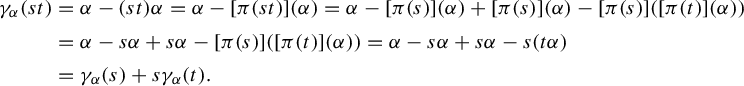 $$ \begin{align*} \gamma_{\alpha} ({s t}) & = \alpha - ({s t}) \alpha = \alpha - [ \pi ({st}) ] ({ \alpha}) = \alpha - [ \pi ({s}) ] ({ \alpha}) + [ \pi ({s}) ] ({ \alpha}) - [ \pi ({s}) ] ({[ \pi ({t}) ] ({ \alpha})}) \\ & = \alpha - s \alpha + s \alpha - [ \pi ({s}) ] ({[ \pi ({t}) ] ({ \alpha})}) = \alpha - s \alpha + s \alpha - s ({t \alpha}) \\ & = \gamma_{\alpha} ({s}) + s \gamma_{ \alpha} ({t}). \end{align*} $$
Hence,
 $ B^{1} ({S,A}) \subseteq Z^{1} ({S,A}) $
. Moreover, we define the first semigroup cohomology of
$ B^{1} ({S,A}) \subseteq Z^{1} ({S,A}) $
. Moreover, we define the first semigroup cohomology of
 $ S $
with coefficients in
$ S $
with coefficients in
 $ A $
by
$ A $
by
 $ H^{1} ({S,A}) := Z^{1} ({S,A}) / B^{1} ({S,A}) $
.
$ H^{1} ({S,A}) := Z^{1} ({S,A}) / B^{1} ({S,A}) $
.
For the special case
 $ S = \mathbb {N}^{k} $
,
$ S = \mathbb {N}^{k} $
,
 $k\in \mathbb {N}_{>0}$
, the following definition provides an important example of an
$k\in \mathbb {N}_{>0}$
, the following definition provides an important example of an
 $ S $
-module.
$ S $
-module.
Definition 3.2. Let
 $ \sigma = ({\sigma _{i}})_{i \in [ k ]} $
be a
$ \sigma = ({\sigma _{i}})_{i \in [ k ]} $
be a
 $ k $
-tuple of commuting surjective local homeomorphisms on the locally compact Hausdorff space
$ k $
-tuple of commuting surjective local homeomorphisms on the locally compact Hausdorff space
 $ X $
. Let
$ X $
. Let
 $ H $
be a topological locally compact abelian group. Define an
$ H $
be a topological locally compact abelian group. Define an
 $ \mathbb {N}^{k} $
-module structure on
$ \mathbb {N}^{k} $
-module structure on
 $ A = \operatorname {C} ({X,H}) $
by setting
$ A = \operatorname {C} ({X,H}) $
by setting
 $$ \begin{align*}[ \pi_{n} ({f}) ] ({x}) := f ({\sigma^{n} ({x})}) \end{align*} $$
for all
 $ n \in \mathbb {N}^{k} $
,
$ n \in \mathbb {N}^{k} $
,
 $ f \in \operatorname {C} ({X,H}) $
, and
$ f \in \operatorname {C} ({X,H}) $
, and
 $ x \in X $
.
$ x \in X $
.
The next condition will be crucial in constructing
 $ 1 $
-cocycles on
$ 1 $
-cocycles on
 $ \mathbb {N}^{k} $
.
$ \mathbb {N}^{k} $
.
Definition 3.3. (Module cocycle condition)
Let
 $ A $
be an
$ A $
be an
 $ \mathbb {N}^{k} $
-module and let
$ \mathbb {N}^{k} $
-module and let
 $ a=({a_{i}})_{i \in [ k ]} $
be a
$ a=({a_{i}})_{i \in [ k ]} $
be a
 $ k $
-tuple of elements of
$ k $
-tuple of elements of
 $ A $
. We say that
$ A $
. We say that
 $ ({a_{i}})_{i \in [ k ]} $
satisfies the module cocycle condition if for all
$ ({a_{i}})_{i \in [ k ]} $
satisfies the module cocycle condition if for all
 $i,j \in [k], ~ i \neq j$
,
$i,j \in [k], ~ i \neq j$
,
 $$ \begin{align} a_{i} + \mathbf{e}_{i} a_{j} = a_{j} + \mathbf{e}_{j} a_{i}, \end{align} $$
where
 $ \{ \mathbf {e}_{i} \}_{i \in [ k ]} $
are the canonical generators of
$ \{ \mathbf {e}_{i} \}_{i \in [ k ]} $
are the canonical generators of
 $ \mathbb {N}^{k} $
.
$ \mathbb {N}^{k} $
.
Theorem 3.4. Let
 $ A $
be an
$ A $
be an
 $ \mathbb {N}^{k} $
-module.
$ \mathbb {N}^{k} $
-module.
-
(1) Suppose that the
$ k $
-tuple
$ a = ({a_{i}})_{i \in [ k ]} \in A^{k} $
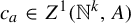
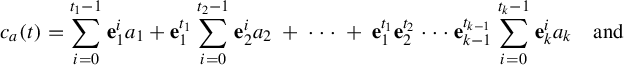
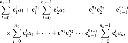
satisfies the module cocycle condition of equation (2). Then there is a unique cocycle
$ c_{a} \in Z^{1} ({\mathbb {N}^{k},A}) $
satisfying, for every
$\ell \in [ k ]$
, (3)The cocycle
$$ \begin{align} c_{a} ({\mathbf{e}_{\ell}}) = a_{\ell}. \end{align} $$
$ c_{a} $
is given by the following formula: (4)
$$ \begin{align} c_{a} ({n}) : = \sum_{i = 0}^{n_{1} - 1} \mathbf{e}_{1}^{i} a_{1} + \mathbf{e}_{1}^{n_{1}} \sum_{i = 0}^{n_{2} - 1} \mathbf{e}_{2}^{i} a_{2}\ + \cdots +\ \mathbf{e}_{1}^{n_{1}} \mathbf{e}_{2}^{n_{2}} \cdots \mathbf{e}_{k - 1}^{n_{k - 1}} \sum_{i = 0}^{n_{k} - 1} \mathbf{e}_{k}^{i} a_{k}. \end{align} $$
-
(2) The correspondence between the
$ k $
-tuples
$ a = ({a_{i}})_{i \in [ k ]} \in A^{k} $
satisfying the module cocycle condition and the associated cocycles
$ c_{a} \in Z^{1} ({\mathbb {N}^{k},A}) $
is a bijection. -
(3) Such a
$ 1 $
-cocycle
$ c_{a} \in Z^{1} ({\mathbb {N}^{k},A}) $
corresponds to a coboundary in
$ B^{1} ({\mathbb {N}^{k},A}) $
if and only there exists
$\alpha \in A$
such that
$ a_{i} = \alpha - \mathbf {e}_{i} \alpha $
for
$ i \in [ k ] $
.


Proof Proof of (1). We subdivide the proof into two parts. We will first prove that the formula for
 $ c_{a} $
in equation (4) gives a
$ c_{a} $
in equation (4) gives a
 $ 1 $
-cocycle on
$ 1 $
-cocycle on
 $ \mathbb {N}^{k} $
satisfying the conditions of equation (3). Then we will prove the uniqueness.
$ \mathbb {N}^{k} $
satisfying the conditions of equation (3). Then we will prove the uniqueness.
For the first part of the proof, we will proceed by induction. For a fixed
 $N\in \mathbb {N}$
our induction statement is that for any
$N\in \mathbb {N}$
our induction statement is that for any
 $t, m,n \in \mathbb {N}^{k} $
, with
$t, m,n \in \mathbb {N}^{k} $
, with
 $ \lvert t \rvert \leq N $
and
$ \lvert t \rvert \leq N $
and
 $ \lvert m + n \rvert \leq N $
, we have
$ \lvert m + n \rvert \leq N $
, we have
 $$ \begin{align} c_{a} ({t}) &= \sum_{i = 0}^{t_{1} - 1} \mathbf{e}_{1}^{i} a_{1} + \mathbf{e}_{1}^{t_{1}} \sum_{i = 0}^{t_{2} - 1} \mathbf{e}_{2}^{i} a_{2}\ +\ \cdots\ +\ \mathbf{e}_{1}^{t_{1}} \mathbf{e}_{2}^{t_{2}} \cdots \mathbf{e}_{k - 1}^{t_{k - 1}} \sum_{i = 0}^{t_{k} - 1} \mathbf{e}_{k}^{i} a_{k}\quad\text{and} \end{align} $$
 $$ \begin{align} c_{a} ({m + n}) &= c_{a} ({m}) + m\ c_{a} ({n}).\end{align} $$
The base case
 $N=1$
is easily checked as it amounts to, for all
$N=1$
is easily checked as it amounts to, for all
 $ \ell \in [ k ] $
,
$ \ell \in [ k ] $
,
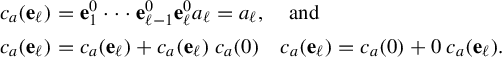 $$ \begin{align*} c_{a} ({\mathbf{e}_{\ell}}) &= \mathbf{e}_{1}^{0} \cdots \mathbf{e}_{\ell -1}^{0} \mathbf{e}_{\ell}^{0} a_{\ell} = a_{\ell},\quad\text{and}\nonumber\\ c_{a} ({\mathbf{e}_{\ell} }) &= c_{a} ({\mathbf{e}_{\ell}}) + c_{a}(\mathbf{e}_{\ell} ) \, c_{a} ({ 0})\quad c_{a} ({\mathbf{e}_{\ell} }) = c_{a} ({0}) +0\, c_{a}(\mathbf{e}_{\ell}). \end{align*} $$
For the inductive step, we now suppose that the cocycle formula in equation (5) holds for all
 $t\in \mathbb {N}^k$
, with
$t\in \mathbb {N}^k$
, with
 $|t|\leq N$
, and that equation (6) holds for all
$|t|\leq N$
, and that equation (6) holds for all
 $n,m\in \mathbb {N}^k$
with
$n,m\in \mathbb {N}^k$
with
 $ |n+m|\leq N$
. We need to show that equation (5) holds for all
$ |n+m|\leq N$
. We need to show that equation (5) holds for all
 $c_a(t)$
, with
$c_a(t)$
, with
 $|t|\leq N+1$
, and that equation (6) holds for all
$|t|\leq N+1$
, and that equation (6) holds for all
 $n,m\in \mathbb {N}^k$
with
$n,m\in \mathbb {N}^k$
with
 $ |n+m|\leq N+1$
. To do so, fix
$ |n+m|\leq N+1$
. To do so, fix
 $m, n \in \mathbb {N}$
with
$m, n \in \mathbb {N}$
with
 $\lvert m +n \rvert = N $
and choose any
$\lvert m +n \rvert = N $
and choose any
 $ \ell \in [ k ] $
so that
$ \ell \in [ k ] $
so that
 $ (m +n +\mathbf {e}_{\ell }) \in \mathbb {N}^k$
, which implies that
$ (m +n +\mathbf {e}_{\ell }) \in \mathbb {N}^k$
, which implies that
 $\lvert m +n +\mathbf {e}_{\ell } \rvert = N + 1 $
.
$\lvert m +n +\mathbf {e}_{\ell } \rvert = N + 1 $
.
Assume first that
 $m =0.$
Then, since
$m =0.$
Then, since
 $|n| = N$
, the induction hypothesis (particularly equation (5)) implies that
$|n| = N$
, the induction hypothesis (particularly equation (5)) implies that
 $$ \begin{align} c_{a} ({\mathbf{e}_{\ell}})\ +\ \mathbf{e}_{\ell}\, c_{a} ({n}) = c_{a} ({\mathbf{e}_{\ell}})\ +\ \mathbf{e}_{\ell} \bigg( \sum_{i = 0}^{n_{1} - 1} \mathbf{e}_{1}^{i} a_{1}\ +\ \cdots \ +\ \mathbf{e}_{1}^{n_{1}} \mathbf{e}_{2}^{n_{2}} \cdots \mathbf{e}_{k - 1}^{n_{k - 1}} \sum_{i = 0}^{n_{k} - 1} \mathbf{e}_{k}^{i} a_{k} \bigg). \end{align} $$
Now note that for
 $ j < \ell $
, the module cocycle condition of equation (2) implies that
$ j < \ell $
, the module cocycle condition of equation (2) implies that
 $$ \begin{align} \mathbf{e}_{\ell} \sum_{i = 0}^{n_{j} - 1} \mathbf{e}_{j}^{i} a_{j} = \sum_{i = 0}^{n_{j} - 1} \mathbf{e}_{j}^{i} ({\mathbf{e}_{\ell} a_{j}}) = \sum_{i = 0}^{n_{j} - 1} \mathbf{e}_{j}^{i} ({a_{j} + \mathbf{e}_{j} a_{\ell} - a_{\ell}}) = \sum_{i = 0}^{n_{j} - 1} \mathbf{e}_{j}^{i} a_{j} + \mathbf{e}_{j}^{n_{j}} a_{\ell} - a_{\ell}. \end{align} $$
Next, we will we use equation (8) to replace the terms
 $ \leq \ell $
in equation (7) with equivalent expressions, to get
$ \leq \ell $
in equation (7) with equivalent expressions, to get
 $$ \begin{align} c_{a} ({\mathbf{e}_{\ell}}) + \mathbf{e}_{\ell} c_{a} ({n}) &= a_{\ell} + \bigg( \sum_{i = 0}^{n_{1} - 1} \mathbf{e}_{1}^{i} a_{1} + \mathbf{e}_{1}^{n_{1}} a_{\ell} - a_{\ell} \bigg)\nonumber\\ &\quad + \mathbf{e}_{1}^{n_{1}} \bigg( \sum_{i = 0}^{n_{2} - 1} \mathbf{e}_{2}^{i} a_{2} + \mathbf{e}_{j}^{n_{j}} a_{\ell} - a_{\ell} \bigg)\nonumber\\ &\quad + \cdots + \mathbf{e}_{1}^{n_{1} - 1} \mathbf{e}_{2}^{n_{2}} \cdots \mathbf{e}_{\ell - 1}^{n_{\ell - 1}} \bigg( \sum_{i=0}^{n_\ell } \textbf{e}_\ell^i(a_\ell) - a_\ell \bigg)\nonumber\\ &\quad+ \cdots + \mathbf{e}_{\ell} \mathbf{e}_{1}^{n_{1} - 1} \mathbf{e}_{2}^{n_{2}} \cdots \mathbf{e}_{k - 1}^{n_{k - 1}} \sum_{i = 0}^{n_{k} - 1} \mathbf{e}_{k}^{i} a_{k}. \end{align} $$
By using the telescopic properties of equation (9) above, one easily sees that
 $ c_{a} ({\mathbf {e}_{\ell }}) + \mathbf {e}_{\ell } c_{a} ({n}) $
is equal to
$ c_{a} ({\mathbf {e}_{\ell }}) + \mathbf {e}_{\ell } c_{a} ({n}) $
is equal to
 $$ \begin{align*} &\sum_{i = 0}^{n_{1} - 1} \mathbf{e}_{1}^{i} a_{1} + \mathbf{e}_{1}^{n_{1}} \sum_{i = 0}^{n_{2} - 1} \mathbf{e}_{2}^{i} a_{2} + \cdots + \mathbf{e}_{1}^{n_{1}} \mathbf{e}_{2}^{n_{2}} \cdots \mathbf{e}_{\ell - 1}^{n_{\ell - 1}}\\ &\quad\times \sum_{i = 0}^{n_{\ell}} \mathbf{e}_{\ell}^{i} a_{\ell} + \cdots + \mathbf{e}_{1}^{n_{1}} \mathbf{e}_{2}^{n_{2}} \cdots \mathbf{e}_{k - 1}^{n_{k - 1}} \sum_{i = 0}^{n_{k} - 1} \mathbf{e}_{k}^{i} a_{k}, \end{align*} $$
which equals
 $ c_{a} ({\mathbf {e}_{\ell } + n})$
. That is, we have proven that, for
$ c_{a} ({\mathbf {e}_{\ell } + n})$
. That is, we have proven that, for
 $n \in \mathbb {N},$
 $\lvert n \rvert = N $
, and any
$\lvert n \rvert = N $
, and any
 $ \ell \in [ k ] $
,
$ \ell \in [ k ] $
,
 $$ \begin{align} c_{a} ({\mathbf{e}_{\ell}})\ +\ \mathbf{e}_{\ell}\, c_{a} ({n})= c_{a} ({\mathbf{e}_{\ell} + n}).\end{align} $$
Moreover, by using equation (5) to replace
 $c_a(n)$
with the right-hand side of that equation in the above expression, a straightforward calculation shows that equation (5) holds for
$c_a(n)$
with the right-hand side of that equation in the above expression, a straightforward calculation shows that equation (5) holds for
 $t=n+ \mathbf {e}_{\ell }.$
We now suppose that
 $ m,n \in \mathbb {N}^{k} $
with
$ m,n \in \mathbb {N}^{k} $
with
 $ \lvert m + n \rvert = N + 1 $
and
$ \lvert m + n \rvert = N + 1 $
and
 $ \lvert m \rvert> 0$
with positive
$ \lvert m \rvert> 0$
with positive
 $\ell $
th coordinate
$\ell $
th coordinate
 $m_\ell $
for some
$m_\ell $
for some
 $ \ell \in [ k ] $
. Define
$ \ell \in [ k ] $
. Define
 $ m' : =\ m- \mathbf {e}_{\ell } \in \mathbb {N}^{k} $
and note that
$ m' : =\ m- \mathbf {e}_{\ell } \in \mathbb {N}^{k} $
and note that
 $ \lvert \mathbf {e}_{\ell } + m' + n \rvert = \lvert m + n \rvert - 1 = ({N + 1}) - 1 = N $
. Therefore, by equation (10), we get
$ \lvert \mathbf {e}_{\ell } + m' + n \rvert = \lvert m + n \rvert - 1 = ({N + 1}) - 1 = N $
. Therefore, by equation (10), we get
 $$ \begin{align*}c_{a} ({m + n}) = c_{a} ({\mathbf{e}_{\ell} + m' + n}) = c_{a} ({\mathbf{e}_{\ell}}) + \mathbf{e}_{\ell}\, c_{a} ({m' + n}). \end{align*} $$
By using the induction hypothesis twice, we now get
 $$\begin{align*} c_{a} ({m + n}) & = c_{a} ({\mathbf{e}_{\ell}}) + \mathbf{e}_{\ell} ({f ({m'}) + m' c_{a} ({n})}) = c_{a} ({\mathbf{e}_{\ell}}) + \mathbf{e}_{\ell} c_{a} ({m'}) + ({\mathbf{e}_{\ell} + m}) c_{a} ({n}) \nonumber\\ & = c_{a} ({\mathbf{e}_{\ell} + m'}) + ({\mathbf{e}_{\ell} + m}) c_{a} ({n}) = c_{a} ({m}) + m\, c_{a} ({n}). \end{align*}$$
Moreover, by using equation (5) to replace in the above expression
 $c_a(m)$
and
$c_a(m)$
and
 $c_a(n)$
with the right-hand side of that equation, a straightforward calculation shows that equation (5) holds for
$c_a(n)$
with the right-hand side of that equation, a straightforward calculation shows that equation (5) holds for
 $t=m+n.$
This completes the inductive step and so we have proven that the formula for
 $ c_{a} $
in equation (4) gives a
$ c_{a} $
in equation (4) gives a
 $ 1 $
-cocycle on
$ 1 $
-cocycle on
 $ \mathbb {N}^{k} $
satisfying the conditions of equation (3).
$ \mathbb {N}^{k} $
satisfying the conditions of equation (3).
We now prove the uniqueness. Let
 $ c_{a} $
be as described above and let
$ c_{a} $
be as described above and let
 $ f $
be any other
$ f $
be any other
 $ 1 $
-cocycle on
$ 1 $
-cocycle on
 $ \mathbb {N}^{k} $
such that
$ \mathbb {N}^{k} $
such that
 $ f ({\mathbf {e}_{i}}) = a_{i} $
for
$ f ({\mathbf {e}_{i}}) = a_{i} $
for
 $ i \in [ k ] $
. Now we proceed by induction on the length
$ i \in [ k ] $
. Now we proceed by induction on the length
 $ \lvert n \rvert $
of n. The base case that
$ \lvert n \rvert $
of n. The base case that
 $ c_{a} ({n}) = f ({n}) $
for all
$ c_{a} ({n}) = f ({n}) $
for all
 $ n \in \mathbb {N}^{k} $
with
$ n \in \mathbb {N}^{k} $
with
 $ \lvert n \rvert \leq 1 $
follows from the definitions of
$ \lvert n \rvert \leq 1 $
follows from the definitions of
 $ c_{a} $
and
$ c_{a} $
and
 $ f $
.
$ f $
.
For the inductive step, assume that
 $ c_{a} ({r}) = f ({r}) $
for all
$ c_{a} ({r}) = f ({r}) $
for all
 $ r \in \mathbb {N}^{k} $
with
$ r \in \mathbb {N}^{k} $
with
 $ \lvert r \rvert \leq N $
and suppose that
$ \lvert r \rvert \leq N $
and suppose that
 $ \lvert n \rvert = n_{1} + n_{2} + \cdots + n_{k} = N $
and
$ \lvert n \rvert = n_{1} + n_{2} + \cdots + n_{k} = N $
and
 $ \lvert m \rvert = m_{1} + m_{2} + \cdots + m_{k} = N + 1 $
, which implies that
$ \lvert m \rvert = m_{1} + m_{2} + \cdots + m_{k} = N + 1 $
, which implies that
 $ m = n + \mathbf {e}_{\ell } $
for some
$ m = n + \mathbf {e}_{\ell } $
for some
 $ \ell $
. By using the inductive hypothesis and the module cocycle condition of equation (2), we then get
$ \ell $
. By using the inductive hypothesis and the module cocycle condition of equation (2), we then get
 $$ \begin{align*}f ({m}) = f ({\mathbf{e}_{\ell} + n}) = c_{a} ({\mathbf{e}_{\ell}}) + \mathbf{e}_{\ell} c_{a} ({n}) = c_{a} ({m}). \end{align*} $$
Proof of (2). We have already proven in (1) that the correspondence
 $a \to c_a$
is injective. To prove that
$a \to c_a$
is injective. To prove that
 $a \to c_a$
is a surjection onto
$a \to c_a$
is a surjection onto
 $ Z^{1} ({\mathbb {N}^{k},A}) $
, let us take
$ Z^{1} ({\mathbb {N}^{k},A}) $
, let us take
 $ c \in Z^{1} ({\mathbb {N}^{k},A}) $
and set
$ c \in Z^{1} ({\mathbb {N}^{k},A}) $
and set
 $ a_{i} := c ({\mathbf {e}_{i}}) $
. It is then easy to check that the
$ a_{i} := c ({\mathbf {e}_{i}}) $
. It is then easy to check that the
 $ k $
-tuple
$ k $
-tuple
 $ ({a_{i}})_{i \in [ k ]} $
satisfies the module cocycle condition.
$ ({a_{i}})_{i \in [ k ]} $
satisfies the module cocycle condition.
Proof of (3). Suppose that the
 $ k $
-tuple
$ k $
-tuple
 $a= ({a_{i}})_{i \in [ k ]} \in A^{k} $
gives rise to a coboundary
$a= ({a_{i}})_{i \in [ k ]} \in A^{k} $
gives rise to a coboundary
 $ c_a $
. Then by definition there exists
$ c_a $
. Then by definition there exists
 $\alpha \in A$
such that for all
$\alpha \in A$
such that for all
 $ i \in [ k ]$
,
$ i \in [ k ]$
,
 $$ \begin{align*}a_{i}= c_{a} ({\mathbf{e}_{i}}) = \alpha - \mathbf{e}_{i} \alpha. \end{align*} $$
The other direction is clear.


3.2 Continuous
$ 1 $
-cocycles on
$ \mathcal {G} ({X,\sigma }) $


In this subsection, our objective is to give an algebraic way of constructing all continuous
 $ H $
-valued
$ H $
-valued
 $ 1 $
-cocycles, where
$ 1 $
-cocycles, where
 $ H $
is a locally compact abelian group, on groupoids associated to a finite family of commuting local homeomorphisms of a compact metric space. In later sections we will mainly be interested in the case
$ H $
is a locally compact abelian group, on groupoids associated to a finite family of commuting local homeomorphisms of a compact metric space. In later sections we will mainly be interested in the case
 $ H = \mathbb {R} $
. We begin by recalling the definition of these groupoids.
$ H = \mathbb {R} $
. We begin by recalling the definition of these groupoids.
Definition 3.6. [Reference Deaconu7, Reference Exel and Renault10]
Let
 $ \sigma = ({\sigma _{i}})_{i \in [ k ]} $
be a
$ \sigma = ({\sigma _{i}})_{i \in [ k ]} $
be a
 $ k $
-tuple of commuting surjective local homeomorphisms on the compact Hausdorff space
$ k $
-tuple of commuting surjective local homeomorphisms on the compact Hausdorff space
 $ X $
. We regard
$ X $
. We regard
 $ \sigma $
as an action of
$ \sigma $
as an action of
 $\mathbb {N}^{k} $
on
$\mathbb {N}^{k} $
on
 $ X $
by the formula
$ X $
by the formula
 $ \sigma ^{n} = \sigma _{1}^{n_{1}} \ldots \sigma _{k}^{n_{k}} $
, where
$ \sigma ^{n} = \sigma _{1}^{n_{1}} \ldots \sigma _{k}^{n_{k}} $
, where
 $ n = ({n_{i}})_{i \in [ k ]} \in N^{k} $
. The transformation groupoid (also called the semidirect product groupoid of the action)
$ n = ({n_{i}})_{i \in [ k ]} \in N^{k} $
. The transformation groupoid (also called the semidirect product groupoid of the action)
 $ \mathcal {G} ({X,\sigma }) $
is defined by
$ \mathcal {G} ({X,\sigma }) $
is defined by
 $$ \begin{align*}\mathcal{G} ({X,\sigma}) := \{ ({x,p - q,y}) \in X \times {\mathbb{Z}}^{k} \times X ~ | ~ p,q \in \mathbb{N}^{k} ~ \text{and} ~ \sigma^{p} ({x}) = \sigma^{q} ({y}) \}. \end{align*} $$
We identify
 $ X $
with the unit space of
$ X $
with the unit space of
 $ \mathcal {G} ({X,\sigma }) $
via the map
$ \mathcal {G} ({X,\sigma }) $
via the map
 $ x \mapsto ({x,0,x}) $
. The structure maps are given by
$ x \mapsto ({x,0,x}) $
. The structure maps are given by
 $ r ({x,n,y}) = x $
,
$ r ({x,n,y}) = x $
,
 $ s ({x,n,y}) = y $
,
$ s ({x,n,y}) = y $
,
 $ ({x,m,y})^{- 1} = ({y,- m,x}) $
, and
$ ({x,m,y})^{- 1} = ({y,- m,x}) $
, and
 $ ({x,m,y}) ({y,n,z}) = ({x,m + n,z}) $
. A basis for the topology on
$ ({x,m,y}) ({y,n,z}) = ({x,m + n,z}) $
. A basis for the topology on
 $ \mathcal {G} ({X,\sigma }) $
is given by subsets of the form
$ \mathcal {G} ({X,\sigma }) $
is given by subsets of the form
 $$ \begin{align*}\mathcal{Z} ({U,V,m,n}) := U \times \{ p - q \} \times V, \end{align*} $$
where
 $ U,V $
are open in
$ U,V $
are open in
 $ X $
and
$ X $
and
 $ \sigma ^{p} [ U ] = \sigma ^{q} [ V ] $
. We will denote by
$ \sigma ^{p} [ U ] = \sigma ^{q} [ V ] $
. We will denote by
 $ \mathcal {G} ({X,\sigma })^{({2})} $
the set of composable pairs of
$ \mathcal {G} ({X,\sigma })^{({2})} $
the set of composable pairs of
 $ \mathcal {G} ({X,\sigma }) $
.
$ \mathcal {G} ({X,\sigma }) $
.
The number
 $ k $
is called the rank of
$ k $
is called the rank of
 $ \mathcal {G} ({X,\sigma }) $
.
$ \mathcal {G} ({X,\sigma }) $
.
It is well known that
 $ \mathcal {G} ({X,\sigma }) $
is an étale locally compact Hausdorff amenable groupoid (cf. [Reference Deaconu7, Reference Renault and Williams26]).
$ \mathcal {G} ({X,\sigma }) $
is an étale locally compact Hausdorff amenable groupoid (cf. [Reference Deaconu7, Reference Renault and Williams26]).
Definition 3.7. (Continuous groupoid 1-cocycles)
Let
 $ \mathcal {G} $
be a topological groupoid and
$ \mathcal {G} $
be a topological groupoid and
 $ H $
be a topological locally compact abelian group. A continuous
$ H $
be a topological locally compact abelian group. A continuous
 $ H $
-valued
$ H $
-valued
 $ 1 $
-cocycle on
$ 1 $
-cocycle on
 $ \mathcal {G} $
is a continuous function
$ \mathcal {G} $
is a continuous function
 $ c: \mathcal {G} \to H $
such that for any
$ c: \mathcal {G} \to H $
such that for any
 $ ({\gamma ,\gamma '}) $
in
$ ({\gamma ,\gamma '}) $
in
 $ \mathcal {G}^{({2})} $
, we have
$ \mathcal {G}^{({2})} $
, we have
 $$ \begin{align*}c ({\gamma \gamma'}) = c ({\gamma}) + c ({\gamma'}). \end{align*} $$
In other words,
 $ c $
is just a continuous groupoid homomorphism from
$ c $
is just a continuous groupoid homomorphism from
 $ \mathcal {G} $
to
$ \mathcal {G} $
to
 $ H $
. We will denote by
$ H $
. We will denote by
 $ Z_{\operatorname {cont}}^{1} ({\mathcal {G},H}) $
the set of continuous
$ Z_{\operatorname {cont}}^{1} ({\mathcal {G},H}) $
the set of continuous
 $ H $
-valued
$ H $
-valued
 $ 1 $
-cocycles on
$ 1 $
-cocycles on
 $ \mathcal {G} $
.
$ \mathcal {G} $
.
It is well known that
 $ Z_{\operatorname {cont}}^{1} ({\mathcal {G},H}) $
is a group under pointwise addition and that
$ Z_{\operatorname {cont}}^{1} ({\mathcal {G},H}) $
is a group under pointwise addition and that
 $ B_{\operatorname {cont}}^{1} ({\mathcal {G},H}) $
, the collection of continuous functions
$ B_{\operatorname {cont}}^{1} ({\mathcal {G},H}) $
, the collection of continuous functions
 $ c: \mathcal {G} \to H $
such that there is a continuous function
$ c: \mathcal {G} \to H $
such that there is a continuous function
 $ f : \mathcal {G}^{({0})} \to H $
such that for all
$ f : \mathcal {G}^{({0})} \to H $
such that for all
 $ \gamma \in \mathcal {G} $
,
$ \gamma \in \mathcal {G} $
,
 $ c ({\gamma }) = f ({r ({\gamma })}) - f ({s ({\gamma })}) $
, is a subgroup of
$ c ({\gamma }) = f ({r ({\gamma })}) - f ({s ({\gamma })}) $
, is a subgroup of
 $ Z_{\operatorname {cont}}^{1} ({\mathcal {G},H}) $
. We define the first continuous cocycle groupoid cohomology of
$ Z_{\operatorname {cont}}^{1} ({\mathcal {G},H}) $
. We define the first continuous cocycle groupoid cohomology of
 $ \mathcal {G} $
by
$ \mathcal {G} $
by
 $$ \begin{align*}H_{\operatorname{cont}}^{1} ({\mathcal{G},H}) := Z_{\operatorname{cont}}^{1} ({\mathcal{G},H}) / B_{\operatorname{cont}}^{1} ({\mathcal{G},H}). \end{align*} $$
Our goal is to give an algebraic characterization of the cocycles in
 $ Z_{\operatorname {cont}}^{1} ({\mathcal {G} ({X,\sigma }),H}) $
for
$ Z_{\operatorname {cont}}^{1} ({\mathcal {G} ({X,\sigma }),H}) $
for
 $ \mathcal {G} ({X,\sigma }) $
expressed in terms of their coordinate-defining functions as given in (2) below. To do so, we will introduce the following definition, which details a special case of the module cocycle condition.
$ \mathcal {G} ({X,\sigma }) $
expressed in terms of their coordinate-defining functions as given in (2) below. To do so, we will introduce the following definition, which details a special case of the module cocycle condition.
Definition 3.8. (The cocycle condition)
Let
 $ H $
be a topological locally compact abelian group. Fix
$ H $
be a topological locally compact abelian group. Fix
 $ k \in \mathbb {N} $
and let
$ k \in \mathbb {N} $
and let
 $ ({X,\sigma ,\varphi }) $
be an ordered triple with:
$ ({X,\sigma ,\varphi }) $
be an ordered triple with:
-
(1)
$ X $
a compact metric space; -
(2)
$ \sigma = ({\sigma _{i}})_{i \in [ k ]} $
a
$ k $
-tuple of commuting surjective local homeomorphisms of
$ X $
; -
(3)
$ \varphi = ({\varphi _{i}})_{i \in [ k ]} $
a
$ k $
-tuple of elements from
$ \operatorname {C} ({X,H}) $
.


Then
 $ ({X,\sigma ,\varphi }) $
is said to satisfy the cocycle condition of order
$ ({X,\sigma ,\varphi }) $
is said to satisfy the cocycle condition of order
 $ k $
if, for all
$ k $
if, for all
 $i,j \in [ k ]$
,
$i,j \in [ k ]$
,
 $$ \begin{align} \varphi_{i} + \varphi_{j} \circ \sigma_{i} = \varphi_{j} + \varphi_{i} \circ \sigma_{j}. \end{align} $$
Note that equation (11) is a special case of the module cocycle condition of Definition 3.3. When the order
 $ k $
is understood, we will omit it and just say that
$ k $
is understood, we will omit it and just say that
 $ ({X,\sigma ,\varphi }) $
satisfies the cocycle condition. Moreover, with a slight abuse of notation, when X and
$ ({X,\sigma ,\varphi }) $
satisfies the cocycle condition. Moreover, with a slight abuse of notation, when X and
 $\sigma $
are understood, we will also say that
$\sigma $
are understood, we will also say that
 $\varphi $
satisfies the cocycle condition.
$\varphi $
satisfies the cocycle condition.
Example 3.9. With notation as in Definition 3.8, if
 $ \varphi _{i} $
is constant for each
$ \varphi _{i} $
is constant for each
 $ i $
, then
$ i $
, then
 $ ({X,\sigma ,\varphi }) $
satisfies the cocycle condition.
$ ({X,\sigma ,\varphi }) $
satisfies the cocycle condition.
The cocycle condition will be the characterizing feature for Ruelle triples in the case of a finite family of commuting endomorphisms; see Definition 4.1.
We now show that every groupoid cocycle
 $ c \in Z_{\operatorname {cont}}^{1} ({\mathcal {G} ({X,\sigma }),H}) $
arises from a
$ c \in Z_{\operatorname {cont}}^{1} ({\mathcal {G} ({X,\sigma }),H}) $
arises from a
 $ k $
-tuple of functions
$ k $
-tuple of functions
 $ ({\varphi _{i}})_{i \in [ k ]} $
satisfying the cocycle condition as above, and conversely.
$ ({\varphi _{i}})_{i \in [ k ]} $
satisfying the cocycle condition as above, and conversely.
Proposition 3.10. (Cocycle characterization)
Let
 $ ({X,\sigma ,\varphi }) $
be a triple that satisfies conditions (1), (2), and (3) of Definition 3.8. Then statements (1) and (2) below are equivalent.
$ ({X,\sigma ,\varphi }) $
be a triple that satisfies conditions (1), (2), and (3) of Definition 3.8. Then statements (1) and (2) below are equivalent.
-
(1) Algebraic characterization:
$ ({X,\sigma ,\varphi }) $
satisfies the cocycle condition. -
(2) There exists a unique
$ c_{X,\sigma ,\varphi } \in Z_{\operatorname {cont}}^{1} ({\mathcal {G} ({X,\sigma }),H}) $
such that
$ c ({x,\mathbf {e}_{i},\sigma _{i} ({x})}) = \varphi _{i} ({x}) $
for all
$ i \in [ k ] $
and
$ x \in X $
.


Moreover, every
 $ c \in Z_{\operatorname {cont}}^{1} ({\mathcal {G} ({X,\sigma }),H}) $
arises as a
$ c \in Z_{\operatorname {cont}}^{1} ({\mathcal {G} ({X,\sigma }),H}) $
arises as a
 $ c_{X,\sigma ,\varphi }$
for some
$ c_{X,\sigma ,\varphi }$
for some
 $k-$
tuple
$k-$
tuple
 $\varphi $
satisfying the cocycle condition. In addition,
$\varphi $
satisfying the cocycle condition. In addition,
 $c \in Z_{\operatorname {cont}}^{1} ({\mathcal {G} ({X,\sigma }),H}) $
is a
$c \in Z_{\operatorname {cont}}^{1} ({\mathcal {G} ({X,\sigma }),H}) $
is a
 $ 1 $
-coboundary if and only if there exists
$ 1 $
-coboundary if and only if there exists
 $ \psi \in \operatorname {C} ({X,H})$
such that
$ \psi \in \operatorname {C} ({X,H})$
such that
 $ c ({x,\mathbf {e}_{i},\sigma _{i} ({x})}) = \psi ({x}) - \psi ({\sigma _{i} ({x})}) $
for all
$ c ({x,\mathbf {e}_{i},\sigma _{i} ({x})}) = \psi ({x}) - \psi ({\sigma _{i} ({x})}) $
for all
 $i,j \in [ k ]$
.
$i,j \in [ k ]$
.
Proof
 $ ({1}) \Longrightarrow ({2}) $
: Assume (1). Since
$ ({1}) \Longrightarrow ({2}) $
: Assume (1). Since
 $ \varphi =({\varphi })_{i \in [ k ]} $
satisfies the cocycle condition, by Proposition 3.4, there is a unique
$ \varphi =({\varphi })_{i \in [ k ]} $
satisfies the cocycle condition, by Proposition 3.4, there is a unique
 $ 1 $
-cocycle
$ 1 $
-cocycle
 $ c_{\varphi } $
on
$ c_{\varphi } $
on
 $ \mathbb {N}^{k} $
, taking values in the
$ \mathbb {N}^{k} $
, taking values in the
 $ \mathbb {N}^{k} $
-module
$ \mathbb {N}^{k} $
-module
 $ \operatorname {C} ({X,H}) $
, that satisfies
$ \operatorname {C} ({X,H}) $
, that satisfies
 $ c ({\mathbf {e}_{i}}) = \varphi _{i} $
for
$ c ({\mathbf {e}_{i}}) = \varphi _{i} $
for
 $ i \in [ k ] $
. Define
$ i \in [ k ] $
. Define
 $ c_{X,\sigma ,\varphi } \in Z_{\operatorname {cont}}^{1} ({\mathcal {G} ({X,\sigma }),H}) $
, for all
$ c_{X,\sigma ,\varphi } \in Z_{\operatorname {cont}}^{1} ({\mathcal {G} ({X,\sigma }),H}) $
, for all
 $m,n \in \mathbb {N}^{k}$
, by
$m,n \in \mathbb {N}^{k}$
, by
 $$ \begin{align*}c_{X,\sigma,\varphi} ({x,m - n,y}) := [ c_{\varphi} ({m}) ] ({x}) - [ c_{\varphi} ({n}) ] ({y}). \end{align*} $$
We must show that
 $ c_{X,\sigma ,\varphi } $
is well defined, that is, if there exist
$ c_{X,\sigma ,\varphi } $
is well defined, that is, if there exist
 $ p,q \in \mathbb {N}^{k} $
with
$ p,q \in \mathbb {N}^{k} $
with
 $ ({x,m - n,y}) = ({x,p - q,y}) \in \mathcal {G} ({X,\sigma }) $
, so that
$ ({x,m - n,y}) = ({x,p - q,y}) \in \mathcal {G} ({X,\sigma }) $
, so that
 $\sigma ^{m} ({x}) = \sigma ^{n} ({y}) $
and
$\sigma ^{m} ({x}) = \sigma ^{n} ({y}) $
and
 $ \sigma ^{p} ({x}) = \sigma ^{q} ({y}) $
, then
$ \sigma ^{p} ({x}) = \sigma ^{q} ({y}) $
, then
 $$ \begin{align*}c_{X,\sigma,\varphi} ({x,m - n,y}) = c_{X,\sigma,\varphi} ({x,p - q,y}). \end{align*} $$
For, note that since
 $ m - n = p - q $
, we have, for all
$ m - n = p - q $
, we have, for all
 $i \in [ k ]$
,
$i \in [ k ]$
,
 $$ \begin{align*}m ({i}) - n ({i}) = p ({i}) - q ({i}), \quad m ({i}) - p ({i}) = n ({i}) - q ({i}). \end{align*} $$
Define
 $ r \in \mathbb {N}^{k} $
by
$ r \in \mathbb {N}^{k} $
by
 $$ \begin{align*} r &= ({r ({1}),r ({2}),\ldots,r ({k})}), \quad \text{where}\\ r ({i})& = \begin{cases} p ({i}) - m ({i}) = q ({i}) - n ({i}) \quad& \text{if} ~ p ({i}) - m ({i})> 0, \\ 0 \quad& \text{if} ~ p ({i}) - m ({i}) \leq 0. \end{cases} \end{align*} $$
It then follows that
 $ m + r = m \vee p $
and
$ m + r = m \vee p $
and
 $ n + r = q \vee p $
, where, for
$ n + r = q \vee p $
, where, for
 $\alpha ,\beta \in \mathbb {N}^k$
, we shall denote by
$\alpha ,\beta \in \mathbb {N}^k$
, we shall denote by
 $ \alpha \vee \beta $
the element of
$ \alpha \vee \beta $
the element of
 $ \mathbb {N}^{k} $
obtained by taking the maximum of the corresponding coordinates in
$ \mathbb {N}^{k} $
obtained by taking the maximum of the corresponding coordinates in
 $ \alpha $
and
$ \alpha $
and
 $ \beta $
. Similarly to r, one can also define
$ \beta $
. Similarly to r, one can also define
 $ t \in \mathbb {N}^{k} $
such that
$ t \in \mathbb {N}^{k} $
such that
 $ p + t = m \vee p $
and
$ p + t = m \vee p $
and
 $ q + t = n \vee q $
. Hence,
$ q + t = n \vee q $
. Hence,
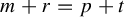 $ m + r = p + t $
and
$ m + r = p + t $
and
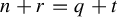 $ n + r = q + t $
.
$ n + r = q + t $
.
We now use the cocycle identity for
 $ c_{\varphi } $
to get, for all
$ c_{\varphi } $
to get, for all
 $ ({x,m - n,y}) = ({x,p - q,y}) \in \mathcal {G} ({X,\sigma }) $
,
$ ({x,m - n,y}) = ({x,p - q,y}) \in \mathcal {G} ({X,\sigma }) $
,
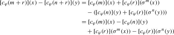 $$ \begin{align*} [ c_{\varphi} ({m + r}) ] ({x}) - [ c_{\varphi} ({n + r}) ] ({y}) & = [ c_{\varphi} ({m}) ] ({x}) + [ c_{\varphi} ({r}) ] ({\sigma^{m} ({x})})\\ &\quad- ({[ c_{\varphi} ({n}) ] ({y}) + [ c_{\varphi} ({r}) ] ({\sigma^{n} ({y})})})\\ & = [ c_{\varphi} ({m}) ] ({x}) - [ c_{\varphi} ({n}) ] ({y})\\ &\quad + [ c_{\varphi} ({r}) ] ({\sigma^{m} ({x})}) - [ c_{\varphi} ({r}) ] ({\sigma^{n} ({y})}) \end{align*} $$
and, because
 $ \sigma ^{m} ({x}) = \sigma ^{n} ({y}) $
, the last two terms cancel each other out.
$ \sigma ^{m} ({x}) = \sigma ^{n} ({y}) $
, the last two terms cancel each other out.
In the same way we show that
 $ [ c_{\varphi } ({p + t}) ] ({x}) - [ c_{\varphi } ({q + t}) ] ({y}) = [ c_{\varphi } ({p}) ] ({x}) - [ c_{\varphi } ({q}) ] ({y}) $
.
$ [ c_{\varphi } ({p + t}) ] ({x}) - [ c_{\varphi } ({q + t}) ] ({y}) = [ c_{\varphi } ({p}) ] ({x}) - [ c_{\varphi } ({q}) ] ({y}) $
.
Therefore,
 $ c_{X,\sigma ,\varphi } ({x,m - n,y}) = c_{X,\sigma ,\varphi } ({x,p - q,y}) $
, so
$ c_{X,\sigma ,\varphi } ({x,m - n,y}) = c_{X,\sigma ,\varphi } ({x,p - q,y}) $
, so
 $ c_{X,\sigma ,\varphi } $
is well defined. Moreover, using the fact that
$ c_{X,\sigma ,\varphi } $
is well defined. Moreover, using the fact that
 $ c_{\varphi } $
is a cocycle, it easily follows that
$ c_{\varphi } $
is a cocycle, it easily follows that
 $ c_{X,\sigma ,\varphi } $
is a cocycle. The fact that
$ c_{X,\sigma ,\varphi } $
is a cocycle. The fact that
 $ c_{X,\sigma ,\varphi } $
is continuous follows from the fact that
$ c_{X,\sigma ,\varphi } $
is continuous follows from the fact that
 $ c_{\varphi } $
takes values in
$ c_{\varphi } $
takes values in
 $ \operatorname {C} ({X,H}) $
.
$ \operatorname {C} ({X,H}) $
.
A straightforward calculation shows that
 $ c_{X,\sigma ,\varphi } $
is unique. Indeed, any
$ c_{X,\sigma ,\varphi } $
is unique. Indeed, any
 $ c \in Z_{\operatorname {cont}}^{1} ({\mathcal {G} ({X,\sigma }),H}) $
is completely determined by
$ c \in Z_{\operatorname {cont}}^{1} ({\mathcal {G} ({X,\sigma }),H}) $
is completely determined by
 $ \varphi _{i} ({x}): = c ({x,\mathbf {e}_{i},\sigma ^{\mathbf {e}_{i}} ({x})}),\ i \in [ k ], $
and
$ \varphi _{i} ({x}): = c ({x,\mathbf {e}_{i},\sigma ^{\mathbf {e}_{i}} ({x})}),\ i \in [ k ], $
and
 $c=c_{X, \sigma ,\varphi }$
, where
$c=c_{X, \sigma ,\varphi }$
, where
 $\varphi =( \varphi _i) $
satisfies the cocycle condition.
$\varphi =( \varphi _i) $
satisfies the cocycle condition.
 $ ({2}) \Longrightarrow ({1})$
: Assume (2). Then we have, for all
$ ({2}) \Longrightarrow ({1})$
: Assume (2). Then we have, for all
 $ i,j \in [ k ] $
and
$ i,j \in [ k ] $
and
 $ x \in X $
, that
$ x \in X $
, that
 $$ \begin{align*} ({x,\mathbf{e}_{i},\sigma_{i} ({x})}) ({\sigma_{i} ({x}),\mathbf{e}_{j},\sigma_{j} ({\sigma_{i} ({x})})}) & = ({x,\mathbf{e}_{i} + \mathbf{e}_{j},\sigma_{j} ({\sigma_{i} ({x})})}) \\ & = ({x,\mathbf{e}_{j} + \mathbf{e}_{i},\sigma_{i} ({\sigma_{j} ({x})})}) \\ & = ({x,\mathbf{e}_{j},\sigma_{j} ({x})}) ({\sigma_{j} ({x}),\mathbf{e}_{i},\sigma_{i} ({\sigma_{j} ({x})})}) \end{align*} $$
and, consequently, for all
 $ x \in X $
,
$ x \in X $
,
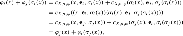 $$ \begin{align*} \varphi_{i} ({x}) + \varphi_{j} ({\sigma_{i} ({x})}) & = c_{X,\sigma,\varphi} ({x,\mathbf{e}_{i},\sigma_{i} ({x})}) + c_{X,\sigma,\varphi} ({\sigma_{i} ({x}),\mathbf{e}_{j},\sigma_{j} ({\sigma_{i} ({x})})}) \\ & = c_{X,\sigma,\varphi} ({({x,\mathbf{e}_{i},\sigma_{i} ({x})}) ({\sigma_{i} ({x}),\mathbf{e}_{j},\sigma_{j} ({\sigma_{i} ({x})})})}) \\ & = c_{X,\sigma,\varphi} ({x,\mathbf{e}_{j},\sigma_{j} ({x})}) + c_{X,\sigma,\varphi} ({\sigma_{j} ({x}),\mathbf{e}_{i},\sigma_{i} ({\sigma_{j} ({x})})}) \\ & = \varphi_{j} ({x}) + \varphi_{i} ({\sigma_{j} ({x})}), \end{align*} $$
which yields (1).
The statement about coboundaries is easily checked.
In the particular setting of a groupoid
 $ \mathcal {G} ({X,\sigma }) $
, with
$ \mathcal {G} ({X,\sigma }) $
, with
 $ A = \operatorname {C} ({X,H}) $
endowed with an
$ A = \operatorname {C} ({X,H}) $
endowed with an
 $\mathbb {N}^k$
-module structure as in Definition 3.2 and Remark 3.5, Theorem 3.4 specializes to outline the relationship between
$\mathbb {N}^k$
-module structure as in Definition 3.2 and Remark 3.5, Theorem 3.4 specializes to outline the relationship between
 $ Z_{\operatorname {cont}}^{1} ({\mathcal {G} ({X,\sigma }),H}) $
and
$ Z_{\operatorname {cont}}^{1} ({\mathcal {G} ({X,\sigma }),H}) $
and
 $\mathbb {N}^k$
-cocycles with values in A.
$\mathbb {N}^k$
-cocycles with values in A.
Corollary 3.11. Let
 $ \mathcal {G} ({X,\sigma }) $
be a groupoid associated to a k-tuple
$ \mathcal {G} ({X,\sigma }) $
be a groupoid associated to a k-tuple
 $\sigma $
of commuting local homeomorphisms of a compact metric space X, and endow
$\sigma $
of commuting local homeomorphisms of a compact metric space X, and endow
 $ A = \operatorname {C} ({X,H}) $
with the structure of an
$ A = \operatorname {C} ({X,H}) $
with the structure of an
 $ \mathbb {N}^{k} $
-module as in Definition 3.2. Then there is an isomorphism
$ \mathbb {N}^{k} $
-module as in Definition 3.2. Then there is an isomorphism
 $$ \begin{align*}\Phi: Z^{1} ({\mathbb{N}^{k},A}) \longrightarrow Z_{\operatorname{cont}}^{1} ({\mathcal{G} ({X,\sigma}),H}),\quad \Phi ({c_{\varphi}}) : = c_{X, \sigma, \varphi}, \end{align*} $$
where, by means of Theorem 3.4,
 $ c_{\varphi } \in Z^{1} ({\mathbb {N}^{k},A}) $
is determined by the
$ c_{\varphi } \in Z^{1} ({\mathbb {N}^{k},A}) $
is determined by the
 $ k $
-tuple
$ k $
-tuple
 $\varphi = ({\varphi _{i}})_{i \in [ k ]} \in A^{k} $
and
$\varphi = ({\varphi _{i}})_{i \in [ k ]} \in A^{k} $
and
 $ c_{X, \sigma , \varphi } $
is the continuous groupoid cocycle associated to
$ c_{X, \sigma , \varphi } $
is the continuous groupoid cocycle associated to
 $ ({X,\sigma ,\varphi }) $
as in Proposition 3.10.
$ ({X,\sigma ,\varphi }) $
as in Proposition 3.10.
Moreover,
 $\Phi $
restricts to an isomorphism between coboundary groups and in addition induces a first cohomology group isomorphism
$\Phi $
restricts to an isomorphism between coboundary groups and in addition induces a first cohomology group isomorphism
 $$ \begin{align*}\overline{\Phi}: H^{1} ({\mathbb{N}^{k},A}) \cong H_{\operatorname{cont}}^{1} ({\mathcal{G} ({X,\sigma}),H}). \end{align*} $$
Proof It is clear that
 $\Phi $
preserves the group operations between
$\Phi $
preserves the group operations between
 $ Z^{1} ({\mathbb {N}^{k},A}) $
and
$ Z^{1} ({\mathbb {N}^{k},A}) $
and
 $ Z_{\operatorname {cont}}^{1} ({\mathcal {G} ({X,\sigma }),H}) $
, and Theorem 3.4 shows that
$ Z_{\operatorname {cont}}^{1} ({\mathcal {G} ({X,\sigma }),H}) $
, and Theorem 3.4 shows that
 $\Phi $
is a bijection. So,
$\Phi $
is a bijection. So,
 $\Phi $
is an isomorphism. It only remains to show that
$\Phi $
is an isomorphism. It only remains to show that
 $\Phi $
induces an isomorphism between
$\Phi $
induces an isomorphism between
 $ B^{1} ({\mathbb {N}^k,A}) $
and
$ B^{1} ({\mathbb {N}^k,A}) $
and
 $B_{\operatorname {cont}}^{1} ({\mathcal {G} ({X,\sigma }),H}) $
. For, assume that
$B_{\operatorname {cont}}^{1} ({\mathcal {G} ({X,\sigma }),H}) $
. For, assume that
 $c_\varphi $
is a coboundary, that is, there exists
$c_\varphi $
is a coboundary, that is, there exists
 $ {f } \in A $
such that
$ {f } \in A $
such that
 $c_\varphi =\gamma _f$
, which implies that
$c_\varphi =\gamma _f$
, which implies that
 $ \varphi _{i} = f - \mathbf {e}_{i} f $
for all
$ \varphi _{i} = f - \mathbf {e}_{i} f $
for all
 $ i \in [ k ] $
. Define, for all
$ i \in [ k ] $
. Define, for all
 $i \in [ k ]$
,
$i \in [ k ]$
,
 $$ \begin{align*}\varphi_{i} ({x}) = f ({x}) - ({\mathbf{e}_{i} f}) ({x}) = f ({x}) - f ({\sigma^{\mathbf{e}_i} ({x})}). \end{align*} $$
Then the cocycle
 $c_f := \Phi (c_\varphi )$
is given by, on
$c_f := \Phi (c_\varphi )$
is given by, on
 $ ({x,l,y}) \in \mathcal {G} ({X,\sigma }) $
for
$ ({x,l,y}) \in \mathcal {G} ({X,\sigma }) $
for
 $ l = m - n $
with
$ l = m - n $
with
 $ \sigma ^{m} ({x}) = \sigma ^{m} ({y}) $
,
$ \sigma ^{m} ({x}) = \sigma ^{m} ({y}) $
,
 $$ \begin{align*}c_{f} ({x,l,y}) = f ({x}) - f ({y}), \end{align*} $$
which is obviously the coboundary corresponding to
 $ f \in \operatorname {C} ({X,H}) $
. It is clear that
$ f \in \operatorname {C} ({X,H}) $
. It is clear that
 $\Phi $
is one-to-one and onto from
$\Phi $
is one-to-one and onto from
 $ B^{1} ({\mathbb {N}^{k},\operatorname {C} ({X,H})}) $
to
$ B^{1} ({\mathbb {N}^{k},\operatorname {C} ({X,H})}) $
to
 $ B_{\operatorname {cont}}^{1} ({\mathcal {G} ({X,\sigma }),H}) $
. By the fundamental theorem for group homomorphisms,
$ B_{\operatorname {cont}}^{1} ({\mathcal {G} ({X,\sigma }),H}) $
. By the fundamental theorem for group homomorphisms,
 $\Phi $
also induces an isomorphism
$\Phi $
also induces an isomorphism
 $$ \begin{align*}H^{1} ({\mathbb{N}^{k},\operatorname{C} ({X,H})}) \cong H_{\operatorname{cont}}^{1} ({\mathcal{G} ({X,\sigma}),H}).\\[-42pt] \end{align*} $$
3.3 Cocycles and Ruelle operators
We now use Proposition 3.10 to deduce properties of Ruelle operators corresponding to
 $ k $
-tuples
$ k $
-tuples
 $\varphi = ({\varphi _{i}})_{i \in [ k ]} $
satisfying the cocycle condition. Recall that by Definition 2.1, the Ruelle operator associated to the Ruelle triple
$\varphi = ({\varphi _{i}})_{i \in [ k ]} $
satisfying the cocycle condition. Recall that by Definition 2.1, the Ruelle operator associated to the Ruelle triple
 $ ({\tilde {X},\tilde {\sigma },\tilde {\phi }}) $
is denoted by
$ ({\tilde {X},\tilde {\sigma },\tilde {\phi }}) $
is denoted by
 $ \mathcal {L}_{\tilde {X},\tilde {\sigma },\tilde {\phi }} $
.
$ \mathcal {L}_{\tilde {X},\tilde {\sigma },\tilde {\phi }} $
.
Theorem 3.12. Let X be a compact Hausdorff space,
 ${\sigma } =( \sigma _i)_{{i \in [ k ]}}$
be a k-tuple of commuting local homeomorphisms of X, and
${\sigma } =( \sigma _i)_{{i \in [ k ]}}$
be a k-tuple of commuting local homeomorphisms of X, and
 $\varphi = ({\varphi _{i}})_{i \in [ k ]} $
be a k-tuple of elements of
$\varphi = ({\varphi _{i}})_{i \in [ k ]} $
be a k-tuple of elements of
 $A=\operatorname {C} ({X,\mathbb {R}})$
.
$A=\operatorname {C} ({X,\mathbb {R}})$
.
-
(1) Assume that
$\varphi $
satisfies the cocycle condition and let
$ c_{\varphi }\in Z^{1} ({\mathbb {N}^{k},A}) $
be the cocycle corresponding to
$\varphi $
as in Theorem 3.4. Then the assignment is a semigroup homomorphism.
$$ \begin{align*} \Psi: \mathbb{N}^{k} \to \operatorname{End} ({\operatorname{C} ({X,\mathbb{R}})}),\quad {\Psi}(n) := \mathcal{L}_{X,\sigma^{n},c_{\varphi} ({n})} \end{align*} $$
-
(2) If the k-tuple of Ruelle operators
$(\mathcal {L}_{X,\sigma ^{\mathbf {e_i}},\varphi _i })_{i \in [ k ]}$
commutes, then
$\varphi $
satisfies the cocycle condition.


Proof For the proof of (1), see Lemma 2.2, which relies on [Reference Exel and Renault10, Proposition 2.2] (this latter reference was pointed out to us by the referee, whom we thank for it).
To prove (2), let
 $ i,j \in [ k ] $
,
$ i,j \in [ k ] $
,
 $ x \in X $
, and
$ x \in X $
, and
 $ z = ({\sigma _{i} \circ \sigma _{j}}) ({x}) $
. As the set
$ z = ({\sigma _{i} \circ \sigma _{j}}) ({x}) $
. As the set
 $$ \begin{align*}S = ({\sigma_{i} \circ \sigma_{j}})^{- 1} [ \{ z \} ] = ({\sigma_{j} \circ \sigma_{i}})^{- 1} [ \{ z \} ] \end{align*} $$
is finite, we can use Urysohn’s lemma to find an
 $ f \in \operatorname {C} ({X,\mathbb {R}}) $
such that
$ f \in \operatorname {C} ({X,\mathbb {R}}) $
such that
 $ f ({x}) = 1 $
and
$ f ({x}) = 1 $
and
 $ f ({y}) = 0 $
for all
$ f ({y}) = 0 $
for all
 $ y \in S \setminus \{ x \} $
. Then
$ y \in S \setminus \{ x \} $
. Then
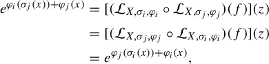 $$ \begin{align*} e^{\varphi_{i} ({\sigma_{j} ({x})}) + \varphi_{j} ({x})} & = [ ({\mathcal{L}_{X,\sigma_{i},\varphi_{i}} \circ \mathcal{L}_{X,\sigma_{j},\varphi_{j}}}) ({f}) ] ({z}) \\ & = [ ({\mathcal{L}_{X,\sigma_{j},\varphi_{j}} \circ \mathcal{L}_{X,\sigma_{i},\varphi_{i}}}) ({f}) ] ({z}) \\ & = e^{\varphi_{j} ({\sigma_{i} ({x})}) + \varphi_{i} ({x})}, \end{align*} $$
which implies that
 $ \varphi _{i} ({\sigma _{j} ({x})}) + \varphi _{j} ({x}) = \varphi _{j} ({\sigma _{i} ({x})}) + \varphi _{i} ({x}) $
. As
$ \varphi _{i} ({\sigma _{j} ({x})}) + \varphi _{j} ({x}) = \varphi _{j} ({\sigma _{i} ({x})}) + \varphi _{i} ({x}) $
. As
 $ x \in X $
is arbitrary, we have proved equation (11).
$ x \in X $
is arbitrary, we have proved equation (11).
4
$ k $
-Ruelle dynamical systems

We now introduce the main objects of our study:
 $ k $
-Ruelle dynamical systems, which are higher-rank analogues of Ruelle triples.
$ k $
-Ruelle dynamical systems, which are higher-rank analogues of Ruelle triples.
Definition 4.1. (k-Ruelle dynamical systems)
A
 $ k $
-Ruelle dynamical system is an ordered triple
$ k $
-Ruelle dynamical system is an ordered triple
 $ ({X,\sigma ,\varphi }) $
that satisfies conditions (1), (2), and (3) of Definition 3.8 and the cocycle condition. For a
$ ({X,\sigma ,\varphi }) $
that satisfies conditions (1), (2), and (3) of Definition 3.8 and the cocycle condition. For a
 $ k $
-Ruelle dynamical system
$ k $
-Ruelle dynamical system
 $ ({X,\sigma ,\varphi }) $
, we will denote by
$ ({X,\sigma ,\varphi }) $
, we will denote by
 $ c_{X,\sigma ,\varphi } $
the unique
$ c_{X,\sigma ,\varphi } $
the unique
 $ c \in Z_{\operatorname {cont}}^{1} ({\mathcal {G} ({X,\sigma }),H}) $
such that for all
$ c \in Z_{\operatorname {cont}}^{1} ({\mathcal {G} ({X,\sigma }),H}) $
such that for all
 $ i \in [ k ] $
and
$ i \in [ k ] $
and
 $ x \in X $
, we have
$ x \in X $
, we have
 $$ \begin{align*}c ({x,\mathbf{e}_{i},\sigma_{i} ({x})}) = \varphi_{i} ({x}). \end{align*} $$
Note that the existence of such a
 $ 1 $
-cocycle is guaranteed by Proposition 3.10.
$ 1 $
-cocycle is guaranteed by Proposition 3.10.
In Definition 4.1, we could have replaced the cocycle condition by any of its equivalent formulations in Proposition 3.10. However, the cocycle condition usually is the easiest of the three equivalent conditions in Proposition 3.10 to verify and work with.
In analogy with triples that satisfy the unique positive eigenvalue condition of Definition 2.3, we have the following definition.
Definition 4.2. A
 $ k $
-Ruelle dynamical system
$ k $
-Ruelle dynamical system
 $ ({X,\sigma ,\varphi }) $
is said to admit a unique solution for the positive eigenvalue problem of the dual of the Ruelle operator if there exists a unique ordered pair
$ ({X,\sigma ,\varphi }) $
is said to admit a unique solution for the positive eigenvalue problem of the dual of the Ruelle operator if there exists a unique ordered pair
 $ ({\boldsymbol {\unicode{x3bb} }^{X,\sigma ,\varphi },\mu ^{X,\sigma ,\varphi }}) $
with the following properties.
$ ({\boldsymbol {\unicode{x3bb} }^{X,\sigma ,\varphi },\mu ^{X,\sigma ,\varphi }}) $
with the following properties.
-
(1)
${\boldsymbol {\unicode{x3bb} }^{X,\sigma ,\varphi } }= ({\unicode{x3bb} _{i}^{X,\sigma ,\varphi }})_{i \in [ k ]} $
is a
$ k $
-tuple of positive real numbers. -
(2)
$ \mu ^{X,\sigma ,\varphi } $
is a Borel probability measure on
$ X $
. -
(3) If
$({\mathcal {L}_{X,\sigma _{i},\varphi _{i}}})^{\ast }$
denotes the dual of the Ruelle operator, then, for each
$ i \in [ k ] $
,


The next result is the
 $ k $
-tuple version of Theorem 2.4.
$ k $
-tuple version of Theorem 2.4.
Theorem 4.3. A
 $ k $
-Ruelle dynamical system
$ k $
-Ruelle dynamical system
 $ ({X,\sigma ,\varphi }) $
satisfies Definition 4.2 if there exists
$ ({X,\sigma ,\varphi }) $
satisfies Definition 4.2 if there exists
 $ n \in \mathbb {N}^{k} \setminus \{ 0 \} $
such that
$ n \in \mathbb {N}^{k} \setminus \{ 0 \} $
such that
 $ ({X,\sigma ^{n},c_{\varphi } ({n})}) $
satisfies the unique positive eigenvalue condition of Definition 2.3.
$ ({X,\sigma ^{n},c_{\varphi } ({n})}) $
satisfies the unique positive eigenvalue condition of Definition 2.3.
Proof Suppose that there is an
 $ n \in \mathbb {N}^{k} \setminus \{ 0 \} $
such that
$ n \in \mathbb {N}^{k} \setminus \{ 0 \} $
such that
 $ ({X,\sigma ^{n},c_{\varphi } ({n})}) $
, with
$ ({X,\sigma ^{n},c_{\varphi } ({n})}) $
, with
 ${\varphi _i=c_{\varphi }}(\mathbf {e_{i}}) $
, is a triple that satisfies the unique positive eigenvalue condition of Definition 2.3. Theorem 3.12 tells us that, for all
${\varphi _i=c_{\varphi }}(\mathbf {e_{i}}) $
, is a triple that satisfies the unique positive eigenvalue condition of Definition 2.3. Theorem 3.12 tells us that, for all
 $i \in [k]$
,
$i \in [k]$
,
 $\mathcal {L}_{X,\sigma ^{\mathbf {e}_{i}},\varphi _{i}} $
and
$\mathcal {L}_{X,\sigma ^{\mathbf {e}_{i}},\varphi _{i}} $
and
 $ \mathcal {L}_{X,\sigma ^{n},c_{\varphi } ({n})} $
commute, which implies that
$ \mathcal {L}_{X,\sigma ^{n},c_{\varphi } ({n})} $
commute, which implies that
 $ \mathcal {L}_{X,\sigma ^{\mathbf {e}_{i}},\varphi _{i}}^{\ast } $
and
$ \mathcal {L}_{X,\sigma ^{\mathbf {e}_{i}},\varphi _{i}}^{\ast } $
and
 $ \mathcal {L}_{X,\sigma ^{n},c_{\varphi } ({n})}^{\ast } $
also commute, and that
$ \mathcal {L}_{X,\sigma ^{n},c_{\varphi } ({n})}^{\ast } $
also commute, and that
 $$ \begin{align*} ({\mathcal{L}_{X,\sigma^{n},c_\varphi ({{n}})}})^{\ast} ({({\mathcal{L}_{X,\sigma_{i},\varphi_{i}}})^{\ast} ({\mu})}) & = ({\mathcal{L}_{X,\sigma_{i},\varphi_{i}}})^{\ast} ({({\mathcal{L}_{X,\sigma^{n},c_\varphi ({{n}})}})^{\ast} ({\mu})}) \\ & = ({\mathcal{L}_{X,\sigma_{i},\varphi_{i}}})^{\ast} ({\unicode{x3bb} \mu}) = \unicode{x3bb} ({\mathcal{L}_{X,\sigma_{i},\varphi_{i}}})^{\ast} ({\mu}). \end{align*} $$
Hence,
 $ ({\mathcal {L}_{X,\sigma _{i},\varphi _{i}}})^{\ast } ({\mu }) $
is an eigenmeasure of
$ ({\mathcal {L}_{X,\sigma _{i},\varphi _{i}}})^{\ast } ({\mu }) $
is an eigenmeasure of
 $ ({\mathcal {L}_{X,\sigma ^{n},c_\varphi ({{n}})}})^{\ast } $
with eigenvalue
$ ({\mathcal {L}_{X,\sigma ^{n},c_\varphi ({{n}})}})^{\ast } $
with eigenvalue
 $ \unicode{x3bb} $
. As we have for all
$ \unicode{x3bb} $
. As we have for all
 $ f \in \operatorname {C} ({X,\mathbb {R}_{\geq 0}}) $
that
$ f \in \operatorname {C} ({X,\mathbb {R}_{\geq 0}}) $
that
 $$ \begin{align*}\int_{X} f ~ \mathrm{d} ({\mathcal{L}_{X,\sigma_{i},\varphi_{i}}})^{\ast} ({\mu}) = \int_{X} \mathcal{L}_{X,\sigma_{i},\varphi_{i}} ({f}) ~ \mathrm{d} \mu \geq 0, \end{align*} $$
it follows that
 $ ({\mathcal {L}_{X,\sigma _{i},\varphi _{i}}})^{\ast } ({\mu }) $
is a non-negative measure on
$ ({\mathcal {L}_{X,\sigma _{i},\varphi _{i}}})^{\ast } ({\mu }) $
is a non-negative measure on
 $ X $
. Furthermore, by the surjectivity of
$ X $
. Furthermore, by the surjectivity of
 $ \sigma _{i} $
,
$ \sigma _{i} $
,
 $$ \begin{align*}\int_{X} 1_{X} ~ \mathrm{d} ({\mathcal{L}_{X,\sigma_{i},\varphi_{i}}})^{\ast} ({\mu}) = \int_{X} \mathcal{L}_{X,\sigma_{i},\varphi_{i}} ({1_{X}}) ~ \mathrm{d} \mu> 0, \end{align*} $$
where we denote by
 $1_{X}$
the characteristic function of X. It follows that
$1_{X}$
the characteristic function of X. It follows that
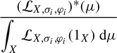 $$ \begin{align*}\frac{({\mathcal{L}_{X,\sigma_{i},\varphi_{i}}})^{\ast} ({\mu})}{\displaystyle \int_{X} \mathcal{L}_{X,\sigma_{i},\varphi_{i}} ({1_{X}}) ~ \mathrm{d} \mu} \end{align*} $$
is a probability eigenmeasure of
 $ ({\mathcal {L}_{X,\sigma ^{n},c_\varphi ({{{n}}})}})^{\ast } $
with eigenvalue
$ ({\mathcal {L}_{X,\sigma ^{n},c_\varphi ({{{n}}})}})^{\ast } $
with eigenvalue
 $ \unicode{x3bb} $
. Since
$ \unicode{x3bb} $
. Since
 $ ({X,\sigma ^{n},c_{\varphi } ({n})}) $
satisfies Definition 2.3, we must have
$ ({X,\sigma ^{n},c_{\varphi } ({n})}) $
satisfies Definition 2.3, we must have
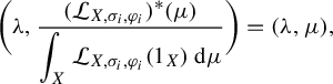 $$ \begin{align*}\bigg({\unicode{x3bb}},{\frac{({\mathcal{L}_{X,\sigma_{i},\varphi_{i}}})^{\ast} ({\mu})}{\displaystyle \int_{X} \mathcal{L}_{X,\sigma_{i},\varphi_{i}} ({1_{X}}) ~ \mathrm{d} \mu}}\bigg) = ({\unicode{x3bb},\mu}), \end{align*} $$
which yields
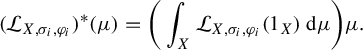 $$ \begin{align*}({\mathcal{L}_{X,\sigma_{i},\varphi_{i}}})^{\ast} ({\mu}) = \bigg( \int_{X} \mathcal{L}_{X,\sigma_{i},\varphi_{i}} ({1_{X}}) ~ \mathrm{d} \mu \bigg) \mu. \end{align*} $$
Now, if
 $ \alpha = ({\alpha _{i}})_{i \in [ k ]} $
is a
$ \alpha = ({\alpha _{i}})_{i \in [ k ]} $
is a
 $ k $
-tuple in
$ k $
-tuple in
 $ \mathbb {R}_{> 0} $
, and
$ \mathbb {R}_{> 0} $
, and
 $ \nu $
a probability Borel measure on
$ \nu $
a probability Borel measure on
 $ X $
such that for all
$ X $
such that for all
 $ i \in [ k ] $
,
$ i \in [ k ] $
,
 $$ \begin{align*}({\mathcal{L}_{X,\sigma_{i},\varphi_{i}}})^{\ast} ({\nu}) = \alpha_{i} \nu, \end{align*} $$
then, by Theorem 3.12, we get, if we set
 $\alpha =(\alpha _1,\ldots , \alpha _k)$
,
$\alpha =(\alpha _1,\ldots , \alpha _k)$
,
 $$ \begin{align*}({\mathcal{L}_{X,\sigma^{n},c_{\varphi} ({n})}})^{\ast} ({\nu}) = \alpha^{n} \nu. \end{align*} $$
As
 $ \alpha ^{n}> 0 $
and
$ \alpha ^{n}> 0 $
and
 $ ({X,\sigma ^{n},c_\varphi ({n})}) $
satisfies Definition 2.3, we also obtain
$ ({X,\sigma ^{n},c_\varphi ({n})}) $
satisfies Definition 2.3, we also obtain
 $ ({\alpha ^{n},\nu }) = ({\unicode{x3bb} ,\mu }) $
, so
$ ({\alpha ^{n},\nu }) = ({\unicode{x3bb} ,\mu }) $
, so
 $ \nu = \mu .$
Hence, for all
$ \nu = \mu .$
Hence, for all
 $ i \in [ k ] $
,
$ i \in [ k ] $
,
 $$ \begin{align*}\alpha_{i} \mu = \bigg( \int_{X} \mathcal{L}_{X,\sigma_{i},\varphi_{i}} ({1_{X}}) ~ \mathrm{d} \mu \bigg) \mu, \end{align*} $$
which yields
 $ \alpha _{i} = \int _{X} \mathcal {L}_{X,\sigma _{i},\varphi _{i}} ({1_{X}}) ~ \mathrm {d} \mu $
for all
$ \alpha _{i} = \int _{X} \mathcal {L}_{X,\sigma _{i},\varphi _{i}} ({1_{X}}) ~ \mathrm {d} \mu $
for all
 $ i \in [ k ] $
.
$ i \in [ k ] $
.
We will now give two examples of
 $ k $
-Ruelle dynamical systems.
$ k $
-Ruelle dynamical systems.
Example 4.4. For
 $ k \in \mathbb {N}_{> 1} $
, let
$ k \in \mathbb {N}_{> 1} $
, let
 $ X := \mathbb {Z}_{k}^{\mathbb {N}_{> 0}} $
be equipped with the product topology, where
$ X := \mathbb {Z}_{k}^{\mathbb {N}_{> 0}} $
be equipped with the product topology, where
 $ {\mathbb {Z}}_{k} := {\mathbb {Z}} / k {\mathbb {Z}} $
. It is well known that the cylinder sets of X form a basis for the topology on X; recall that every finite word
$ {\mathbb {Z}}_{k} := {\mathbb {Z}} / k {\mathbb {Z}} $
. It is well known that the cylinder sets of X form a basis for the topology on X; recall that every finite word
 $\alpha \in ({\mathbb {Z}}_k)^m$
defines an associated cylinder set
$\alpha \in ({\mathbb {Z}}_k)^m$
defines an associated cylinder set
 $\mathcal {Z}[\alpha ]$
by
$\mathcal {Z}[\alpha ]$
by
 $$ \begin{align*}\mathcal{Z}[\alpha] : = \{x\in X\ |\ (x_j)_{j=1,\ldots, m}= \alpha \}.\end{align*} $$
Define a commuting
 $ k $
-tuple
$ k $
-tuple
 $ \sigma = ({\sigma _{i}})_{i \in [ k ]} $
of surjective local homeomorphisms on
$ \sigma = ({\sigma _{i}})_{i \in [ k ]} $
of surjective local homeomorphisms on
 $ X $
by
$ X $
by
 $$ \begin{align*}\text{for all } i \in [ k ]\quad\text{for all } x \in X: \sigma_{i} ({x}) := ({x_{n + 1} + ({i - 1})})_{n \in \mathbb{N}_{> 0}}. \end{align*} $$
We want to verify Definition 2.5. To do so, we first check that
 $ \sigma _{i} $
is positively expansive and exact for each
$ \sigma _{i} $
is positively expansive and exact for each
 $ i \in [ k ] $
, and subsequently verify that
$ i \in [ k ] $
, and subsequently verify that
 $ \varphi $
is Hölder-continuous.
$ \varphi $
is Hölder-continuous.
A straightforward calculation shows that, if we define
 $ U :=\{ ({x,y}) \in X \times X ~ | ~ x_{1} = y_{1} \} $
, then
$ U :=\{ ({x,y}) \in X \times X ~ | ~ x_{1} = y_{1} \} $
, then
 $$ \begin{align*}\Delta ({X}) \subseteq U = \bigcup_{i \in [ k ]} \mathcal{Z}[i] \times \mathcal{Z}[i]. \end{align*} $$
To deduce that
 $ \sigma _{i} $
is positively expansive for each
$ \sigma _{i} $
is positively expansive for each
 $ i \in [ k ] $
, simply observe that if
$ i \in [ k ] $
, simply observe that if
 $ x,y \in X $
are distinct, then
$ x,y \in X $
are distinct, then
 $ ({\sigma _{i}^{m - 1} ({x}),\sigma _{i}^{m - 1} ({y})}) \notin U $
, where
$ ({\sigma _{i}^{m - 1} ({x}),\sigma _{i}^{m - 1} ({y})}) \notin U $
, where
 $ m := \min ({\{ n \in \mathbb {N}_{> 0} ~ | ~ x_{n} \neq y_{n} \}}) $
.
$ m := \min ({\{ n \in \mathbb {N}_{> 0} ~ | ~ x_{n} \neq y_{n} \}}) $
.
Now we will show that
 $ \sigma _{i} $
is exact for each
$ \sigma _{i} $
is exact for each
 $ i \in [ k ] $
. Let
$ i \in [ k ] $
. Let
 $U \subseteq X$
be a non-empty open set. Since the cylinder sets form a basis for the topology on X, there is a cylinder set
$U \subseteq X$
be a non-empty open set. Since the cylinder sets form a basis for the topology on X, there is a cylinder set
 $\mathcal {Z}[\alpha ] \subseteq U,$
with
$\mathcal {Z}[\alpha ] \subseteq U,$
with
 $|\alpha |=m,$
for some
$|\alpha |=m,$
for some
 $m \in \mathbb {N}_{>0}.$
Then
$m \in \mathbb {N}_{>0}.$
Then
 $ \sigma _{i}^{m} [ U ] \supset \sigma _{i}^{m} [ \mathcal {Z}[\alpha ] ]= X $
, which means that
$ \sigma _{i}^{m} [ U ] \supset \sigma _{i}^{m} [ \mathcal {Z}[\alpha ] ]= X $
, which means that
 $ \sigma _{i} $
is exact for each
$ \sigma _{i} $
is exact for each
 $ i \in [ k ] $
.
$ i \in [ k ] $
.
Let
 $ d: X \times X\to \mathbb {R}_{\geq 0} $
denote the compatible metric on
$ d: X \times X\to \mathbb {R}_{\geq 0} $
denote the compatible metric on
 $ X $
defined by, for all
$ X $
defined by, for all
 $x,y \in X$
,
$x,y \in X$
,
 $$ \begin{align*}d ({x,y}) := 2^{- \min ({\{ n \in \mathbb{N}_{> 0} ~ | ~ x_{n} \neq y_{n} \}})}, \end{align*} $$
where
 $ \min ({\varnothing }) := \infty $
by convention.
$ \min ({\varnothing }) := \infty $
by convention.
Now let
 $ ({a_{i}})_{i \in [ k ]} \in \mathbb {R}^{k} $
and define
$ ({a_{i}})_{i \in [ k ]} \in \mathbb {R}^{k} $
and define
 $ \varphi : X \to \mathbb {R} $
by, for all
$ \varphi : X \to \mathbb {R} $
by, for all
 $i \in [ k ],~\text {for all } x \in X$
,
$i \in [ k ],~\text {for all } x \in X$
,
 $$ \begin{align*}\varphi ({x}) := a_{i} \iff \sum_{n = 1}^{k} x_{n} = i - 1 ~ ({\text{mod}~k}). \end{align*} $$
Clearly,
 $ \varphi $
is continuous. Indeed, we note that the value of
$ \varphi $
is continuous. Indeed, we note that the value of
 $ \varphi $
at
$ \varphi $
at
 $ x\in X $
depends only on the first
$ x\in X $
depends only on the first
 $ k $
components of
$ k $
components of
 $ x $
, so that if
$ x $
, so that if
 $ x,y \in X$
and
$ x,y \in X$
and
 $ d ({x,y}) < 2^{- k} $
, then
$ d ({x,y}) < 2^{- k} $
, then
 $ \varphi ({x}) = \varphi ({y}) $
, so that
$ \varphi ({x}) = \varphi ({y}) $
, so that
 $ \lvert \varphi ({x}) - \varphi ({y}) \rvert = 0 $
in that case. One therefore computes, for all
$ \lvert \varphi ({x}) - \varphi ({y}) \rvert = 0 $
in that case. One therefore computes, for all
 $ x,y \in X $
,
$ x,y \in X $
,
 $$ \begin{align*}\lvert \varphi ({x}) - \varphi ({y}) \rvert \leq 2^{k} ({\max_{i,j \in [ k ]} \lvert a_{i} - a_{j} \rvert}) d ({x,y}), \end{align*} $$
which implies that
 $ \varphi $
is Hölder-continuous with respect to
$ \varphi $
is Hölder-continuous with respect to
 $ d $
.
$ d $
.
Let
 $ ({c_{i}})_{i \in [ k ]} \in \mathbb {R}^{k} $
. Then, for all
$ ({c_{i}})_{i \in [ k ]} \in \mathbb {R}^{k} $
. Then, for all
 $ i,j \in [ k ] $
and for all
$ i,j \in [ k ] $
and for all
 $ x \in X $
,
$ x \in X $
,
 $$ \begin{align*}({\varphi + c_{i} 1_{X}}) ({\sigma_{j} ({x})}) - ({\varphi + c_{j} 1_{X}}) ({\sigma_{i} ({x})}) \kern1.3pt{=}\kern1.3pt ({\varphi ({\sigma_{i} ({x})}) + c_{i}}) - ({\varphi ({\sigma_{j} ({x})}) + c_{j}}) \kern1.3pt{=}\kern1.3pt c_{i} - c_{j}, \end{align*} $$
the final equality holding because
 $ \varphi ({\sigma _{i} ({x})}) = \varphi ({\sigma _{j} ({x})}) $
. Therefore,
$ \varphi ({\sigma _{i} ({x})}) = \varphi ({\sigma _{j} ({x})}) $
. Therefore,
 $(X,({\sigma _{i}})_{i \in [ k ]}, ({\varphi + c_{i} 1_{X}})_{i \in [ k ]}) $
is a Ruelle dynamical system and, since the Ruelle triple
$(X,({\sigma _{i}})_{i \in [ k ]}, ({\varphi + c_{i} 1_{X}})_{i \in [ k ]}) $
is a Ruelle dynamical system and, since the Ruelle triple
 $ ({X,\sigma _{i},\varphi _{i}}) $
satisfies the conditions of Definition 2.5 for each
$ ({X,\sigma _{i},\varphi _{i}}) $
satisfies the conditions of Definition 2.5 for each
 $ i \in [ k ] $
, we conclude that
$ i \in [ k ] $
, we conclude that
 $ (X,({\sigma _{i}})_{i \in [ k ]}, ({\varphi + c_{i} 1_{X}})_{i \in [ k ]}) $
satisfies the unique positive eigenvalue condition of Definition 2.3.
$ (X,({\sigma _{i}})_{i \in [ k ]}, ({\varphi + c_{i} 1_{X}})_{i \in [ k ]}) $
satisfies the unique positive eigenvalue condition of Definition 2.3.
The next example exhibits a dynamical system on a non-Cantor space admitting a unique solution to the positive eigenvalue problem.
Example 4.5. Let
 $ n = ({n_{i}})_{i \in [ k ]} $
be a
$ n = ({n_{i}})_{i \in [ k ]} $
be a
 $ k $
-tuple,
$ k $
-tuple,
 $ n_{i} \in {\mathbb {Z}} \setminus \{ 0,\pm 1 \} $
, and define a commuting
$ n_{i} \in {\mathbb {Z}} \setminus \{ 0,\pm 1 \} $
, and define a commuting
 $ k $
-tuple
$ k $
-tuple
 $ \sigma = ({\sigma _{i}})_{i \in [ k ]} $
of surjective local homeomorphisms on
$ \sigma = ({\sigma _{i}})_{i \in [ k ]} $
of surjective local homeomorphisms on
 $ \mathbb {T} $
by, for all
$ \mathbb {T} $
by, for all
 $i \in [ k ]$
and for all
$i \in [ k ]$
and for all
 $z \in \mathbb {T}$
,
$z \in \mathbb {T}$
,
 $\sigma _{i} ({z}) := z^{n_{i}}.$
The local homeomorphism
$\sigma _{i} ({z}) := z^{n_{i}}.$
The local homeomorphism
 $ \sigma _{i} $
is expansive for each
$ \sigma _{i} $
is expansive for each
 $ i \in [ k ] $
by [Reference Shub29, top of p. 176]. Now let
$ i \in [ k ] $
by [Reference Shub29, top of p. 176]. Now let
 $ U $
be a non-empty open subset of
$ U $
be a non-empty open subset of
 $ \mathbb {T} $
. Then there exist
$ \mathbb {T} $
. Then there exist
 $ \alpha ,\beta \in \mathbb {R} $
such that
$ \alpha ,\beta \in \mathbb {R} $
such that
 $ \alpha < \beta $
and
$ \alpha < \beta $
and
 $$ \begin{align*}\{ e^{\textrm{i} \theta} \in \mathbb{T} ~ | ~ \alpha < \theta < \beta \} \subseteq U. \end{align*} $$
Let
 $ i \in [ k ] $
and let
$ i \in [ k ] $
and let
 $ m \in \mathbb {N} $
be such that
$ m \in \mathbb {N} $
be such that
 $ 2 \pi \leq m \lvert n_{i} \rvert ({\beta - \alpha }) $
. Then
$ 2 \pi \leq m \lvert n_{i} \rvert ({\beta - \alpha }) $
. Then
 $$ \begin{align*} \sigma_{i}^{m} [ U ] & \supseteq \sigma_{i}^{m} [ \{ e^{\textrm{i} \theta} \in \mathbb{T} ~ | ~ \alpha < \theta < \beta \} ] = \{ e^{\textrm{i} m n_{i} \theta} \in \mathbb{T} ~ | ~ \alpha < \theta < \beta \} \\ & = \{ e^{\textrm{i} \theta} \in \mathbb{T} ~ | ~ \theta ~ \text{between} ~ m n_{i} \alpha ~ \text{and} ~ m n_{i} \beta \} = \mathbb{T}, \end{align*} $$
so
 $ \sigma _{i} $
is exact.
$ \sigma _{i} $
is exact.
Let
 $ d $
denote the metric on
$ d $
denote the metric on
 $ \mathbb {T} $
, defined by, for all
$ \mathbb {T} $
, defined by, for all
 $ \alpha ,\beta \in \mathbb {R} $
,
$ \alpha ,\beta \in \mathbb {R} $
,
 $$ \begin{align*}d(e^{i\alpha},e^{i\beta})= \text{inf}\{|\alpha-(\beta+n\pi)| : n\in\mathbb Z\}.\end{align*} $$
The metric
 $ d $
generates the standard topology on
$ d $
generates the standard topology on
 $ \mathbb {T} $
.
$ \mathbb {T} $
.
Define a
 $ k $
-tuple
$ k $
-tuple
 $ \varphi = ({\varphi _{i}})_{i \in [ k ]} $
in
$ \varphi = ({\varphi _{i}})_{i \in [ k ]} $
in
 $ \operatorname {C} ({X,\mathbb {C}}) $
by, for all
$ \operatorname {C} ({X,\mathbb {C}}) $
by, for all
 $i \in [ k ], ~ \text { for all } z \in \mathbb {T}$
,
$i \in [ k ], ~ \text { for all } z \in \mathbb {T}$
,
 $\varphi _{i} ({z}) = z^{n_{i}} - z.$
A straightforward calculation shows that
$\varphi _{i} ({z}) = z^{n_{i}} - z.$
A straightforward calculation shows that
 $ \varphi _{i} $
is Hölder-continuous with respect to
$ \varphi _{i} $
is Hölder-continuous with respect to
 $ d $
for each
$ d $
for each
 $ i \in [ k ] $
and that the (
$ i \in [ k ] $
and that the (
 $ \mathbb {C} $
-valued) cocycle condition
$ \mathbb {C} $
-valued) cocycle condition
 $ \varphi _{i} + \varphi _{j} \circ \sigma _{i} = \varphi _{j} + \varphi _{i} \circ \sigma _{j}$
holds.
$ \varphi _{i} + \varphi _{j} \circ \sigma _{i} = \varphi _{j} + \varphi _{i} \circ \sigma _{j}$
holds.
Now let
 $ f: \mathbb {C} \to \mathbb {R} $
be a continuous additive map (e.g.,
$ f: \mathbb {C} \to \mathbb {R} $
be a continuous additive map (e.g.,
 $ f ({z}) = {\mathrm {Re}}(z) $
). As
$ f ({z}) = {\mathrm {Re}}(z) $
). As
 $ f $
is then Hölder-continuous with respect to the Euclidean metrics on
$ f $
is then Hölder-continuous with respect to the Euclidean metrics on
 $ \mathbb {C} $
and
$ \mathbb {C} $
and
 $ \mathbb {R} $
,
$ \mathbb {R} $
,
 $ f \circ \varphi _{i} $
is also Hölder-continuous with respect to
$ f \circ \varphi _{i} $
is also Hölder-continuous with respect to
 $ d $
and, by the additivity of
$ d $
and, by the additivity of
 $ f $
, for every
$ f $
, for every
 $i,j \kern1.2pt{\in}\kern1.2pt [ k ] $
,
$i,j \kern1.2pt{\in}\kern1.2pt [ k ] $
,
 $$ \begin{align*} ({f \circ \varphi_{i}}) + ({f \circ \varphi_{j}}) \circ \sigma_{i} &= f \circ ({\varphi_{i} + \varphi_{j} \circ \sigma_{i}}) = f \circ ({\varphi_{j} + \varphi_{i} \circ \sigma_{j}})\\ &= ({f \circ \varphi_{j}}) + ({f \circ \varphi_{i}}) \circ \sigma_{j}, \end{align*} $$
so that
 $ ({\mathbb {T},\sigma ,({f \circ \varphi _{i}})_{i \in [ k ]}}) $
is a Ruelle dynamical system. As the Ruelle triple
$ ({\mathbb {T},\sigma ,({f \circ \varphi _{i}})_{i \in [ k ]}}) $
is a Ruelle dynamical system. As the Ruelle triple
 $ ({\mathbb {T},\sigma _{i},f \circ \varphi _{i}}) $
satisfies the conditions in Definition 2.5 for each
$ ({\mathbb {T},\sigma _{i},f \circ \varphi _{i}}) $
satisfies the conditions in Definition 2.5 for each
 $ i \in [ k ] $
, we conclude that
$ i \in [ k ] $
, we conclude that
 $ ({\mathbb {T},\sigma ,({f \circ \varphi _{i}})_{i \in [ k ]}}) $
has a unique eigenmeasure as in Definition 4.2.
$ ({\mathbb {T},\sigma ,({f \circ \varphi _{i}})_{i \in [ k ]}}) $
has a unique eigenmeasure as in Definition 4.2.
Example 4.6. Fixing
 $ d \in \mathbb {N} $
, where
$ d \in \mathbb {N} $
, where
 $ d> 1 $
, define two commuting local homeomorphisms
$ d> 1 $
, define two commuting local homeomorphisms
 $ \sigma _{1} $
and
$ \sigma _{1} $
and
 $ \sigma _{2} $
of
$ \sigma _{2} $
of
 $ \mathbb {T}^{2} $
by, for all
$ \mathbb {T}^{2} $
by, for all
 $z_{1},z_{2} \in \mathbb {T}$
,
$z_{1},z_{2} \in \mathbb {T}$
,
 $$ \begin{align*}\sigma_{1} ({z_{1},z_{2}}) := ({z_{1}^{d},z_{2}^{d}}), \quad \sigma_{2} ({z_{1},z_{2}}) := ({z_{1} z_{2}^{- 1},z_{1} z_{2}}). \end{align*} $$
Since all the eigenvalues of the associated matrices
 $ M_{\sigma _{1}} := \big [\begin {smallmatrix} d & 0 \\ 0 & d \end {smallmatrix}\big ] $
and
$ M_{\sigma _{1}} := \big [\begin {smallmatrix} d & 0 \\ 0 & d \end {smallmatrix}\big ] $
and
 $ M_{\sigma _{2}} := \big [\begin {smallmatrix} 1 & - 1 \\ 1 & 1 \end {smallmatrix}\big ] $
have modulus larger than one,
$ M_{\sigma _{2}} := \big [\begin {smallmatrix} 1 & - 1 \\ 1 & 1 \end {smallmatrix}\big ] $
have modulus larger than one,
 $ \sigma _{1} $
and
$ \sigma _{1} $
and
 $ \sigma _{2} $
are toral endomorphisms that are positively expansive and exact (see [Reference Mihaelescu19, Proof of Theorem 1]). In this case, we can choose the functions
$ \sigma _{2} $
are toral endomorphisms that are positively expansive and exact (see [Reference Mihaelescu19, Proof of Theorem 1]). In this case, we can choose the functions
 $ \varphi _{j} := c_{j} 1_{\mathbb {T}^{2}} $
to be constant functions. Therefore, the Ruelle triple
$ \varphi _{j} := c_{j} 1_{\mathbb {T}^{2}} $
to be constant functions. Therefore, the Ruelle triple
 $ ({\mathbb {T}^{2},\sigma _{i},c_{i} 1_{\mathbb {T}^{2}}}) $
satisfies the conditions of Definition 2.5 for each
$ ({\mathbb {T}^{2},\sigma _{i},c_{i} 1_{\mathbb {T}^{2}}}) $
satisfies the conditions of Definition 2.5 for each
 $ i \in \{ 1,2 \} $
.
$ i \in \{ 1,2 \} $
.
The next example is a combination of Examples 4.5 and 4.4.
Example 4.7. Let
 $ X := {\mathbb {Z}}_{k}^{\mathbb {N}_{> 0}} $
with
$ X := {\mathbb {Z}}_{k}^{\mathbb {N}_{> 0}} $
with
 $ k \in \mathbb {N}_{> 1} $
. Fixing
$ k \in \mathbb {N}_{> 1} $
. Fixing
 $ I \in [ k ] $
and
$ I \in [ k ] $
and
 $ J \in \mathbb {N}_{> 1} $
, define local homeomorphisms
$ J \in \mathbb {N}_{> 1} $
, define local homeomorphisms
 $ \sigma _{I},\sigma _{J}: X \times \mathbb {T} \to X \times \mathbb {T} $
by the following formula. For all
$ \sigma _{I},\sigma _{J}: X \times \mathbb {T} \to X \times \mathbb {T} $
by the following formula. For all
 $ ({x,z}) \in X \times \mathbb {T} $
, set
$ ({x,z}) \in X \times \mathbb {T} $
, set
 $$\begin{align*}\sigma_{I} ({x,z}) & := ({({x_{n + 1} + ({I - 1})})_{n \in \mathbb{N}_{> 0}},z}), \nonumber\\ \sigma_{J} ({x,z}) & := ({x,z^{J}}).\end{align*}$$
It is clear that
 $ \sigma _{I} $
and
$ \sigma _{I} $
and
 $ \sigma _{J} $
commute and one calculates that the composition
$ \sigma _{J} $
commute and one calculates that the composition
 $ \sigma _{I} \circ \sigma _{J} $
is positively expansive and exact. By proceeding as in Examples 4.5 and 4.4, and using Theorem 4.3 with
$ \sigma _{I} \circ \sigma _{J} $
is positively expansive and exact. By proceeding as in Examples 4.5 and 4.4, and using Theorem 4.3 with
 $ k = 2 $
and
$ k = 2 $
and
 $ ({n_{1},n_{2}}) = ({1,1}) $
, the resulting Ruelle triple satisfies the conditions in Definition 2.5.
$ ({n_{1},n_{2}}) = ({1,1}) $
, the resulting Ruelle triple satisfies the conditions in Definition 2.5.
Example 4.8. We will now compute Ruelle eigenvalues and eigenmeasures for the
 $ k $
-Ruelle dynamical system
$ k $
-Ruelle dynamical system
 $ ({X,\sigma ,\varphi }) $
, with
$ ({X,\sigma ,\varphi }) $
, with
 $ X = \prod _{j \in \mathbb {N}} \{ 0,1 \} $
, where
$ X = \prod _{j \in \mathbb {N}} \{ 0,1 \} $
, where
 $ \{ 0,1 \} = {\mathbb {Z}}_2 $
, and
$ \{ 0,1 \} = {\mathbb {Z}}_2 $
, and
 $ \sigma = ({\sigma _{1},\sigma _{2}}) $
is defined by, for
$ \sigma = ({\sigma _{1},\sigma _{2}}) $
is defined by, for
 $ x = ({x_{n}})_{n \in \mathbb {N}} $
,
$ x = ({x_{n}})_{n \in \mathbb {N}} $
,
 $$ \begin{align*}\sigma_{1} ({x}) := ({x_{n + 1}})_{n \in \mathbb{N}}, \quad \sigma_{2} ({x}) := ({x_{n} + 1})_{n \in \mathbb{N}}. \end{align*} $$
Moreover, for
 $ a,b,c \in \mathbb {R} $
, define
$ a,b,c \in \mathbb {R} $
, define
 $ \varphi = ({\varphi _{1},\varphi _{2}}) $
by the following equation, where below addition is considered modulo two:
$ \varphi = ({\varphi _{1},\varphi _{2}}) $
by the following equation, where below addition is considered modulo two:
 $$ \begin{align} \varphi_{1} ({x}) := \begin{cases} a \quad& \text{if} ~ x_{0} + x_{1} = 0, \\ b \quad& \text{if} ~ x_{0} + x_{1} = 1, \end{cases} \quad \varphi_{2} ({x}) := c. \end{align} $$
Firstly, it is a simple exercise to determine that the eigenvalues
 $ \unicode{x3bb} _{1},\unicode{x3bb} _{2} $
of the associated Ruelle operator are given by
$ \unicode{x3bb} _{1},\unicode{x3bb} _{2} $
of the associated Ruelle operator are given by
 $ \unicode{x3bb} _{1} = e^{a} +e^{b} $
and
$ \unicode{x3bb} _{1} = e^{a} +e^{b} $
and
 $ \unicode{x3bb} _{2} = e^{c} $
, and that
$ \unicode{x3bb} _{2} = e^{c} $
, and that
 $ \mu ({Z ({0})}) = \mu ({Z ({1})}) = \tfrac 12 $
.
$ \mu ({Z ({0})}) = \mu ({Z ({1})}) = \tfrac 12 $
.
Moreover, the eigenmeasure
 $ \mu $
on all of the cylinder sets can be computed by using induction, thus proving that
$ \mu $
on all of the cylinder sets can be computed by using induction, thus proving that
 $ \mu $
is defined on the cylinder sets of
$ \mu $
is defined on the cylinder sets of
 $ X $
according to the following probability diagram and formula. We leave the details of this calculation to the reader.
$ X $
according to the following probability diagram and formula. We leave the details of this calculation to the reader.
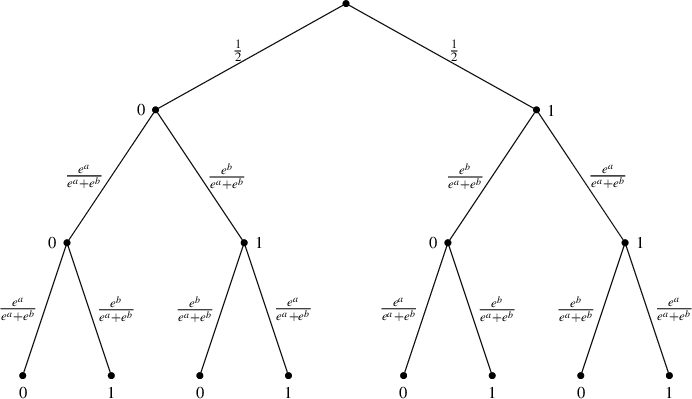
 $$ \begin{align} \mu ({Z ({x_{0} x_{1} \cdots x_{n}})}) = \frac{1}{2} \prod_{j = 0}^{n - 1} \frac{e^{\psi ({x_{j} + x_{j + 1}})}}{e^{a} +e^{b}}, \end{align} $$
where
 $ \psi : \{ 0,1 \} \to \{ a,b \} $
is defined by
$ \psi : \{ 0,1 \} \to \{ a,b \} $
is defined by
 $ \psi ({0}) := a $
and
$ \psi ({0}) := a $
and
 $ \psi ({1}) := b $
.
$ \psi ({1}) := b $
.
In the above formula, note that when
 $ n = 0 $
, the resulting product is empty and so by convention equal to
$ n = 0 $
, the resulting product is empty and so by convention equal to
 $ 1 $
. Therefore,
$ 1 $
. Therefore,
 $ \mu ({Z ({x_{0}})}) = \tfrac 12 $
for all
$ \mu ({Z ({x_{0}})}) = \tfrac 12 $
for all
 $ x_{0} \in \{ 0,1 \} $
.
$ x_{0} \in \{ 0,1 \} $
.
5 The Radon–Nikodym problem and KMS states
This section addresses the Radon–Nikodym problem for groupoids associated to a finite family of commuting local homeomorphisms of a compact metric space, which provides a link between quasi-invariant measures for these groupoids and KMS states for a generalized gauge dynamics on the associated
 $ C^{\ast } $
-algebra. As a result, there will be a heavier emphasis on measure theory and topology than the previous sections.
$ C^{\ast } $
-algebra. As a result, there will be a heavier emphasis on measure theory and topology than the previous sections.
Definition 5.1. (Pull-back and quasi-invariant measures)
Let
 $ \mu $
be a Borel probability measure defined on the Borel sets of the compact metric space
$ \mu $
be a Borel probability measure defined on the Borel sets of the compact metric space
 $ X $
with associated Borel
$ X $
with associated Borel
 $ \sigma $
-algebra
$ \sigma $
-algebra
 $ \mathscr {B} ({X}) $
and let
$ \mathscr {B} ({X}) $
and let
 $ \sigma = ({\sigma _{i}})_{i \in [ k ]} $
be a commuting
$ \sigma = ({\sigma _{i}})_{i \in [ k ]} $
be a commuting
 $ k $
-tuple of surjective local homeomorphisms on
$ k $
-tuple of surjective local homeomorphisms on
 $ X $
. Define regular Borel measures
$ X $
. Define regular Borel measures
 $ s^{\ast } \mu $
and
$ s^{\ast } \mu $
and
 $ r^{\ast } \mu $
on
$ r^{\ast } \mu $
on
 $ \mathcal {G} ({X,\sigma }) $
by, for all
$ \mathcal {G} ({X,\sigma }) $
by, for all
 $ B \in \mathscr {B} ({\mathcal {G} ({X,\sigma })}) $
,
$ B \in \mathscr {B} ({\mathcal {G} ({X,\sigma })}) $
,
 $$ \begin{align*} ({s^{\ast} \mu}) ({B}) & := \int_{X} \bigg( \sum_{\gamma \in \mathcal{G} ({X,\sigma})_{x}} 1_{B} ({\gamma}) \bigg) ~ \mathrm{d} \mu ({x}), \\ ({r^{\ast} \mu}) ({B}) & := \int_{X} \bigg( \sum_{\gamma \in \mathcal{G} ({X,\sigma})^{x}} 1_{B} ({\gamma}) \bigg) ~ \mathrm{d} \mu ({x}), \end{align*} $$
where we denote by
 $ \mathcal {G} ({X,\sigma })_{x} $
(respectively
$ \mathcal {G} ({X,\sigma })_{x} $
(respectively
 $ \mathcal {G} ({X,\sigma })^{x} $
) the set of arrows in
$ \mathcal {G} ({X,\sigma })^{x} $
) the set of arrows in
 $ \mathcal {G} ({X,\sigma }) $
with source
$ \mathcal {G} ({X,\sigma }) $
with source
 $ x $
(respectively range
$ x $
(respectively range
 $ x $
). We then say that
$ x $
). We then say that
 $ \mu $
is quasi-invariant for
$ \mu $
is quasi-invariant for
 $ \mathcal {G} ({X,\sigma })$
if
$ \mathcal {G} ({X,\sigma })$
if
 $ s^{\ast } \mu $
and
$ s^{\ast } \mu $
and
 $ r^{\ast } \mu $
are equivalent to one another, in which case a Radon–Nikodym derivative for
$ r^{\ast } \mu $
are equivalent to one another, in which case a Radon–Nikodym derivative for
 $ \mu $
is any measurable function on
$ \mu $
is any measurable function on
 $ \mathcal {G} ({X,\sigma }) $
in the same equivalence class (with respect to the equivalence relation module sets of measure zero) as
$ \mathcal {G} ({X,\sigma }) $
in the same equivalence class (with respect to the equivalence relation module sets of measure zero) as
 ${\mathrm {d} r^{\ast } \mu }/{\mathrm {d} s^{\ast } \mu }$
[Reference Renault22, §3].
${\mathrm {d} r^{\ast } \mu }/{\mathrm {d} s^{\ast } \mu }$
[Reference Renault22, §3].
The following lemma will be used in the proof of Theorem 5.3. Its proof follows from the definition of local homeomorphism and the fact that
 $ X $
is compact.
$ X $
is compact.
Lemma 5.2. Let
 $ T: X \to Y $
be a local homeomorphism of topological spaces from the compact metric space
$ T: X \to Y $
be a local homeomorphism of topological spaces from the compact metric space
 $ X $
to the metric space
$ X $
to the metric space
 $ Y $
. Then
$ Y $
. Then
 $ \sup _{y \in Y} \textsf {Card} ({T^{- 1} [ \{ y \} ]}) < \infty $
.
$ \sup _{y \in Y} \textsf {Card} ({T^{- 1} [ \{ y \} ]}) < \infty $
.
The following theorem is a generalization of Proposition 4.2 of [Reference Renault24] from Deaconu–Renault groupoids to groupoids
 $ \mathcal {G} ({X,\sigma }) $
and characterizes the solutions of the Radon–Nykodym problem in this general setting. Its proof is quite technical, although in part it is possible to rely on the steps given in Renault’s proof in [Reference Renault24].
$ \mathcal {G} ({X,\sigma }) $
and characterizes the solutions of the Radon–Nykodym problem in this general setting. Its proof is quite technical, although in part it is possible to rely on the steps given in Renault’s proof in [Reference Renault24].
Theorem 5.3. Let
 $ ({X,\sigma ,\varphi }) $
be a
$ ({X,\sigma ,\varphi }) $
be a
 $ k $
-Ruelle dynamical system, which satisfies the conditions of Definition 4.2, and
$ k $
-Ruelle dynamical system, which satisfies the conditions of Definition 4.2, and
 $ \mu $
a Borel probability measure on
$ \mu $
a Borel probability measure on
 $ X $
. Then the following statements are equivalent.
$ X $
. Then the following statements are equivalent.
-
(1)
$ \mu $
is quasi-invariant for
$\mathcal {G} ({X,\sigma }) $
and the Radon–Nikodym derivative
$ {\mathrm {d} r^{\ast } \mu }/{\mathrm {d} s^{\ast } \mu } $
is the continuous function
$ e^{c_{X,\sigma ,\varphi }} $
on
$ \mathcal {G} ({X,\sigma }) $
. -
(2)
$ ({\mathcal {L}_{X,\sigma _{i},\varphi _{i}}})^{\ast } ({\mu }) = \mu $
for each
$ i \in [ k ] $
.


Proof Assume that (1) holds and fix
 $ i \in [ k ] $
; then
$ i \in [ k ] $
; then
 $ \mu $
is quasi-invariant for the subgroupoid
$ \mu $
is quasi-invariant for the subgroupoid
 $$ \begin{align*}\mathcal{G} ({X,\sigma_{i}}) := \{ ({x,\ell \mathbf{e}_{i},y}) ~ | ~ x,y \in X, ~ m,n \in \mathbb{N}, ~ \ell = m - n, ~ \sigma_{i}^{m} ({x}) = \sigma_{i}^{n} ({y}) \} \end{align*} $$
of
 $ \mathcal {G} ({X,\sigma }) $
determined by the singly generated system
$ \mathcal {G} ({X,\sigma }) $
determined by the singly generated system
 $ ({X,\sigma _{i}}) $
. Thus, by Proposition 4.2 of [Reference Renault24] and using its notation, we have that
$ ({X,\sigma _{i}}) $
. Thus, by Proposition 4.2 of [Reference Renault24] and using its notation, we have that
 $^{t}\mathcal {L}_{\varphi _i} ({\mu }) = \mu ,$
which in our notation means that
$^{t}\mathcal {L}_{\varphi _i} ({\mu }) = \mu ,$
which in our notation means that
 $ ({\mathcal {L}_{X,\sigma _{i},\varphi _{i}}})^{\ast } ({\mu }) = \mu $
. So,
$ ({\mathcal {L}_{X,\sigma _{i},\varphi _{i}}})^{\ast } ({\mu }) = \mu $
. So,
 $ ({1}) \Longrightarrow ({2})$
.
$ ({1}) \Longrightarrow ({2})$
.
Conversely, assume that (2) holds. We first briefly explain why
 $ \mu $
is quasi-invariant for
$ \mu $
is quasi-invariant for
 $ \mathcal {G} ({X,\sigma }) $
. A straightforward calculation shows that for all
$ \mathcal {G} ({X,\sigma }) $
. A straightforward calculation shows that for all
 $ i \in [ k ] $
,
$ i \in [ k ] $
,
 $ f \in \operatorname {C} ({X,\mathbb {R}}) $
, and
$ f \in \operatorname {C} ({X,\mathbb {R}}) $
, and
 $ x \in X $
, we have
$ x \in X $
, we have
 $$ \begin{gather*} \int_{X} f ~ \mathrm{d} ({({\sigma_{i}})_{\ast} \mu}) = \int_{X} f \mathcal{L}_{X,\sigma_{i},\varphi_{i}} ({1_{X}}) ~ \mathrm{d} \mu. \end{gather*} $$
The Riesz representation theorem then implies that for all
 $ A \in \mathscr {B} ({X}) $
,
$ A \in \mathscr {B} ({X}) $
,
 $$ \begin{align*}({({\sigma_{i}})_{\ast} \mu}) ({A}) = \int_{X} 1_{A} \mathcal{L}_{X,\sigma_{i},\varphi_{i}} ({1_{X}}) ~ \mathrm{d} \mu, \end{align*} $$
which yields
 $ ({\sigma _{i}})_{\ast } \mu = \mu \circ \sigma _{i}^{- 1} \ll \mu $
for
$ ({\sigma _{i}})_{\ast } \mu = \mu \circ \sigma _{i}^{- 1} \ll \mu $
for
 $ i \in [ k ] $
. On the other hand,
$ i \in [ k ] $
. On the other hand,
 $ \mu \ll \mu \circ \sigma _{i}^{- 1} $
for
$ \mu \ll \mu \circ \sigma _{i}^{- 1} $
for
 $ i \in [ k ] $
by Proposition 4.2 of [Reference Renault24]. By Lemma 5.2, we now get that for all
$ i \in [ k ] $
by Proposition 4.2 of [Reference Renault24]. By Lemma 5.2, we now get that for all
 $ B \in \mathscr {B} ({\mathcal {G} ({X,\sigma })}) $
and some
$ B \in \mathscr {B} ({\mathcal {G} ({X,\sigma })}) $
and some
 $N\in \mathbb {N}_{>0}$
,
$N\in \mathbb {N}_{>0}$
,
 $$ \begin{align*}\mu ({s [ B ]}) \leq ({s^{\ast} \mu}) ({B}) \leq N \mu ({s [ B ]}), \end{align*} $$
which implies that
 $ \mu ({s [ B ]}) = 0 $
if and only if
$ \mu ({s [ B ]}) = 0 $
if and only if
 $ ({s^{\ast } \mu }) ({B}) = 0 $
; using a similar technique, we can also prove that
$ ({s^{\ast } \mu }) ({B}) = 0 $
; using a similar technique, we can also prove that
 $ \mu ({r [ B ]}) = 0 $
if and only if
$ \mu ({r [ B ]}) = 0 $
if and only if
 $ ({r^{\ast } \mu }) ({B}) = 0 $
. Finally, by the monotonicity and countable additivity of
$ ({r^{\ast } \mu }) ({B}) = 0 $
. Finally, by the monotonicity and countable additivity of
 $ \mu $
, we have for all
$ \mu $
, we have for all
 $ B \in \mathscr {B} ({\mathcal {G} ({X,\sigma })}) $
that
$ B \in \mathscr {B} ({\mathcal {G} ({X,\sigma })}) $
that
 $$ \begin{align*}\mu ({s [ B ]}) \leq {\mu}\bigg({\bigcup_{m,n \in \mathbb{N}^{k}} ({\sigma^{m}})^{- 1} [ \sigma^{n} [ r [ B ] ] ]}\bigg) = 0, \end{align*} $$
so that if
 $ \mu ({r [ B ]}) = 0 $
, then
$ \mu ({r [ B ]}) = 0 $
, then
 $ \mu ({s [ B ]}) = 0 $
, and the same method shows that if
$ \mu ({s [ B ]}) = 0 $
, and the same method shows that if
 $ \mu ({s [ B ]}) = 0 $
, then
$ \mu ({s [ B ]}) = 0 $
, then
 $ \mu ({r [ B ]}) = 0 $
. All of these facts taken together imply that for a fixed
$ \mu ({r [ B ]}) = 0 $
. All of these facts taken together imply that for a fixed
 $ B \in \mathscr {B} ({\mathcal {G} ({X,\sigma })}) $
, we have
$ B \in \mathscr {B} ({\mathcal {G} ({X,\sigma })}) $
, we have
 $ ({r^{\ast } \mu }) ({B}) = 0 $
if and only if
$ ({r^{\ast } \mu }) ({B}) = 0 $
if and only if
 $ ({s^{\ast } \mu }) ({B}) = 0 $
, so
$ ({s^{\ast } \mu }) ({B}) = 0 $
, so
 $ r^{\ast } \mu $
and
$ r^{\ast } \mu $
and
 $ s^{\ast } \mu $
are equivalent Borel measures on
$ s^{\ast } \mu $
are equivalent Borel measures on
 $ \mathcal {G} ({X,\sigma }) $
. Therefore,
$ \mathcal {G} ({X,\sigma }) $
. Therefore,
 $ \mu $
is quasi-invariant for
$ \mu $
is quasi-invariant for
 $ \mathcal {G} ({X,\sigma }) $
.
$ \mathcal {G} ({X,\sigma }) $
.
Now, by (2), we have for all
 $ f \in \operatorname {C} ({X,\mathbb {R}}) $
and every
$ f \in \operatorname {C} ({X,\mathbb {R}}) $
and every
 $ i \in [ k ] ,$
that
$ i \in [ k ] ,$
that
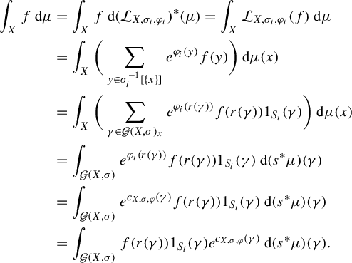 $$ \begin{align*} \int_{X} f ~ \mathrm{d} \mu & = \int_{X} f ~ \mathrm{d} ({\mathcal{L}_{X,\sigma_{i},\varphi_{i}}})^{\ast} ({\mu}) = \int_{X} \mathcal{L}_{X,\sigma_{i},\varphi_{i}} ({f}) ~ \mathrm{d} \mu \\ & = \int_{X} \bigg( \sum_{y \in \sigma_{i}^{- 1} [ \{ x \} ]} e^{\varphi_{i} ({y})} f ({y}) \bigg) ~ \mathrm{d} \mu ({x}) \\ & = \int_{X} \bigg( \sum_{\gamma \in \mathcal{G} ({X,\sigma})_{x}} e^{\varphi_{i} ({r ({\gamma})})} f ({r ({\gamma})}) 1_{S_{i}} ({\gamma}) \bigg) ~ \mathrm{d} \mu ({x}) \\ & = \int_{\mathcal{G} ({X,\sigma})} e^{\varphi_{i} ({r ({\gamma})})} f ({r ({\gamma})}) 1_{S_{i}} ({\gamma}) ~ \mathrm{d} ({s^{\ast} \mu}) ({\gamma}) \\ & = \int_{\mathcal{G} ({X,\sigma})} e^{c_{X,\sigma,\varphi} ({\gamma})} f ({r ({\gamma})}) 1_{S_{i}} ({\gamma}) ~ \mathrm{d} ({s^{\ast} \mu}) ({\gamma}) \\ & = \int_{\mathcal{G} ({X,\sigma})} f ({r ({\gamma})}) 1_{S_{i}} ({\gamma}) e^{c_{X,\sigma,\varphi} ({\gamma})} ~ \mathrm{d} ({s^{\ast} \mu}) ({\gamma}). \end{align*} $$
From the above equations, it follows that the Radon–Nikodym derivative of
 $ r^{\ast } \mu $
with respect to
$ r^{\ast } \mu $
with respect to
 $ s^{\ast } \mu $
must be equal to
$ s^{\ast } \mu $
must be equal to
 $ e^{c_{X,\sigma ,\varphi } ({\gamma })} $
for almost all
$ e^{c_{X,\sigma ,\varphi } ({\gamma })} $
for almost all
 $ \gamma \in S_{i} $
. By [Reference Renault22, Proposition I.3.3],
$ \gamma \in S_{i} $
. By [Reference Renault22, Proposition I.3.3],
 $ D $
is a measurable
$ D $
is a measurable
 $ \mathbb {R}\setminus \{0\} $
-valued
$ \mathbb {R}\setminus \{0\} $
-valued
 $ 1 $
-cocycle on
$ 1 $
-cocycle on
 $ \mathcal {G} ({X,\sigma }),$
and
$ \mathcal {G} ({X,\sigma }),$
and
 $ D =_{\operatorname {a.e.}} e^{c_{X,\sigma ,\varphi }} $
, which is continuous by assumption. Therefore,
$ D =_{\operatorname {a.e.}} e^{c_{X,\sigma ,\varphi }} $
, which is continuous by assumption. Therefore,
 $ e^{c_{X,\sigma ,\varphi }} $
is a continuous Radon–Nikodym cocycle associated to the quasi-invariant measure
$ e^{c_{X,\sigma ,\varphi }} $
is a continuous Radon–Nikodym cocycle associated to the quasi-invariant measure
 $ \mu $
and we have established
$ \mu $
and we have established
 $ ({2}) \Longrightarrow ({1}) $
.
$ ({2}) \Longrightarrow ({1}) $
.
We now illustrate a particular problem of existence of KMS states arising in the context of
 $ \mathcal {G} ({X,\sigma })$
. In the following example there are no KMS states associated to the dynamics, even though one of the associated local homeomorphisms acting on X is expansive and exact.
$ \mathcal {G} ({X,\sigma })$
. In the following example there are no KMS states associated to the dynamics, even though one of the associated local homeomorphisms acting on X is expansive and exact.
Example 5.4. Recall that the Cuntz algebra
 $ \mathcal {O}_{N} $
, where
$ \mathcal {O}_{N} $
, where
 $ N \geq 2 $
, is the
$ N \geq 2 $
, is the
 $ C^{\ast } $
-algebra associated to the groupoid arising from the action of the standard shift
$ C^{\ast } $
-algebra associated to the groupoid arising from the action of the standard shift
 $ \sigma _{N} $
on
$ \sigma _{N} $
on
 $ X_{N} := \prod _{j \in \mathbb {N}} [ N ] $
. In [Reference Olesen and Pedersen21], Olesen and Pedersen proved that for
$ X_{N} := \prod _{j \in \mathbb {N}} [ N ] $
. In [Reference Olesen and Pedersen21], Olesen and Pedersen proved that for
 $N \geq 2$
there is exactly one KMS state for
$N \geq 2$
there is exactly one KMS state for
 $ \mathcal {O}_{N} $
with respect to the canonical gauge action
$ \mathcal {O}_{N} $
with respect to the canonical gauge action
 $ \alpha _{N} $
of
$ \alpha _{N} $
of
 $ \mathbb {R} $
on
$ \mathbb {R} $
on
 $ \mathcal {O}_{N} $
associated to the cocycle determined by
$ \mathcal {O}_{N} $
associated to the cocycle determined by
 $ \varphi _{N} = 1 $
. This KMS state arises at the inverse temperature value
$ \varphi _{N} = 1 $
. This KMS state arises at the inverse temperature value
 $ \beta = \ln ({N}) $
.
$ \beta = \ln ({N}) $
.
Now take
 $ X = X_{2} \times X_{3} $
and define
$ X = X_{2} \times X_{3} $
and define
 $ \sigma = ({\sigma _{2},\sigma _{3}}) $
, where
$ \sigma = ({\sigma _{2},\sigma _{3}}) $
, where
 $ \sigma _{j} $
is the standard shift on
$ \sigma _{j} $
is the standard shift on
 $ X_{j} $
; also, set
$ X_{j} $
; also, set
 $ \varphi = ({\varphi _{2},\varphi _{3}}) $
with
$ \varphi = ({\varphi _{2},\varphi _{3}}) $
with
 $\varphi _{2} = 1$
and
$\varphi _{2} = 1$
and
 $\varphi _{3} = 1$
. Note that the shift corresponding to
$\varphi _{3} = 1$
. Note that the shift corresponding to
 $ ({1,1}) \in \mathbb {N}^{2} $
is expansive and exact. Consider the automorphism group
$ ({1,1}) \in \mathbb {N}^{2} $
is expansive and exact. Consider the automorphism group
 $ \alpha = \alpha _{2} \otimes \alpha _{3} $
defined on the
$ \alpha = \alpha _{2} \otimes \alpha _{3} $
defined on the
 $ C^{\ast } $
-algebra corresponding to
$ C^{\ast } $
-algebra corresponding to
 $ ({X,\sigma ,\varphi }) $
, which is the tensor product
$ ({X,\sigma ,\varphi }) $
, which is the tensor product
 $ \mathcal {O}_{2} \otimes \mathcal {O}_{3} $
of the
$ \mathcal {O}_{2} \otimes \mathcal {O}_{3} $
of the
 $ C^{\ast } $
-algebras
$ C^{\ast } $
-algebras
 $ \mathcal {O}_{2}$
and
$ \mathcal {O}_{2}$
and
 $\mathcal {O}_{3} $
. Suppose that for some
$\mathcal {O}_{3} $
. Suppose that for some
 $ \beta \in \mathbb {R} $
, there is a state
$ \beta \in \mathbb {R} $
, there is a state
 $ \omega $
on this tensor product
$ \omega $
on this tensor product
 $ C^{\ast } $
-algebra that satisfies the KMS condition for the automorphism group
$ C^{\ast } $
-algebra that satisfies the KMS condition for the automorphism group
 $ \alpha $
. Then, by the Olesen–Pedersen result,
$ \alpha $
. Then, by the Olesen–Pedersen result,
 $ \omega $
restricted to the
$ \omega $
restricted to the
 $ C^{\ast } $
-subalgebra
$ C^{\ast } $
-subalgebra
 $ \mathcal {O}_{2} \otimes \mathbb {C} \operatorname {Id}_{\mathcal {O}_{3}} $
satisfies the KMS condition for
$ \mathcal {O}_{2} \otimes \mathbb {C} \operatorname {Id}_{\mathcal {O}_{3}} $
satisfies the KMS condition for
 $ \alpha $
only at
$ \alpha $
only at
 $ \beta = \ln ({2}) $
, whereas
$ \beta = \ln ({2}) $
, whereas
 $ \omega $
restricted to the subalgebra
$ \omega $
restricted to the subalgebra
 $ \mathbb {C} \operatorname {Id}_{\mathcal {O}_{2}} \otimes \mathcal {O}_{3} $
satisfies the KMS condition for
$ \mathbb {C} \operatorname {Id}_{\mathcal {O}_{2}} \otimes \mathcal {O}_{3} $
satisfies the KMS condition for
 $ \alpha $
only at
$ \alpha $
only at
 $ \beta = \ln ({3}) $
. Therefore, by the aforementioned result of Olesen and Pedersen [Reference Olesen and Pedersen21], there cannot be any KMS states for the
$ \beta = \ln ({3}) $
. Therefore, by the aforementioned result of Olesen and Pedersen [Reference Olesen and Pedersen21], there cannot be any KMS states for the
 $ C^{\ast } $
-algebra
$ C^{\ast } $
-algebra
 $ \mathcal {O}_{2} \otimes \mathcal {O}_{3} $
associated to
$ \mathcal {O}_{2} \otimes \mathcal {O}_{3} $
associated to
 $ ({X,\sigma ,\varphi }) $
for the automorphism group
$ ({X,\sigma ,\varphi }) $
for the automorphism group
 $ \alpha = \alpha _{1} \otimes \alpha _{2} $
.
$ \alpha = \alpha _{1} \otimes \alpha _{2} $
.
We are now in a position to introduce the generalized gauge dynamics of a
 $ k $
-Ruelle dynamical system, which satisfies the conditions of Definition 4.2.
$ k $
-Ruelle dynamical system, which satisfies the conditions of Definition 4.2.
Definition 5.5. (Generalized gauge dynamics)
The generalized gauge dynamics of a
 $ k $
-Ruelle dynamical system
$ k $
-Ruelle dynamical system
 $ ({X,\sigma ,\varphi }) $
, which satisfies the conditions of Definition 4.2, is by definition the
$ ({X,\sigma ,\varphi }) $
, which satisfies the conditions of Definition 4.2, is by definition the
 $ \mathbb {R} $
-dynamical system
$ \mathbb {R} $
-dynamical system
 $ ({C^{\ast } ({\mathcal {G} ({X,\sigma })}),\alpha ^{X,\sigma ,\varphi }}) $
defined by
$ ({C^{\ast } ({\mathcal {G} ({X,\sigma })}),\alpha ^{X,\sigma ,\varphi }}) $
defined by
 $$ \begin{align*}({\alpha^{X,\sigma,\varphi}_{t} ({f})}) ({\gamma}) := e^{i t c_{X,\sigma,\varphi} ({\gamma})} f ({\gamma}) \end{align*} $$
for all
 $ f \in \operatorname {C_{c}} ({\mathcal {G} ({X,\sigma })}) $
,
$ f \in \operatorname {C_{c}} ({\mathcal {G} ({X,\sigma })}) $
,
 $ \gamma \in {\mathcal {G} ({X,\sigma })} $
, and
$ \gamma \in {\mathcal {G} ({X,\sigma })} $
, and
 $ t \in \mathbb {R} $
, where here we are implicitly using the canonical embedding of
$ t \in \mathbb {R} $
, where here we are implicitly using the canonical embedding of
 $ \operatorname {C_{c}} ({\mathcal {G} ({X,\sigma })}) $
into
$ \operatorname {C_{c}} ({\mathcal {G} ({X,\sigma })}) $
into
 $ C^{\ast }_{\textrm {r}} ({\mathcal {G} ({X,\sigma })}) $
.
$ C^{\ast }_{\textrm {r}} ({\mathcal {G} ({X,\sigma })}) $
.
The following result may be found in [Reference Renault22]; see also the discussion preceding Proposition 3.2 of [Reference Kumjian and Renault17].
Proposition 5.6. [Reference Renault22]
Let
 $ ({X,\sigma ,\varphi }) $
be a
$ ({X,\sigma ,\varphi }) $
be a
 $ k $
-Ruelle dynamical system that satisfies the conditions of Definition 4.2 and let
$ k $
-Ruelle dynamical system that satisfies the conditions of Definition 4.2 and let
 $ \beta \in \mathbb {R} $
. Then, for every quasi-invariant measure
$ \beta \in \mathbb {R} $
. Then, for every quasi-invariant measure
 $ \mu $
for
$ \mu $
for
 $ ({X,\sigma }) $
with continuous Radon–Nikodym derivative
$ ({X,\sigma }) $
with continuous Radon–Nikodym derivative
 $ e^{- \beta c_{X,\sigma ,\varphi }} $
, there exists a
$ e^{- \beta c_{X,\sigma ,\varphi }} $
, there exists a
 $ \operatorname {KMS}_{\beta } $
-state
$ \operatorname {KMS}_{\beta } $
-state
 $ \omega $
for the generalized gauge dynamics of
$ \omega $
for the generalized gauge dynamics of
 $ ({X,\sigma ,\varphi }) $
that is uniquely determined by
$ ({X,\sigma ,\varphi }) $
that is uniquely determined by
 $$ \begin{align*}\omega ({f}) = \int_{X} f ({x,0,x}) ~ \mathrm{d} \mu \end{align*} $$
for all
 $ f \in \operatorname {C_{c}} ({\mathcal {G} ({X,\sigma })}) $
.
$ f \in \operatorname {C_{c}} ({\mathcal {G} ({X,\sigma })}) $
.
It is not necessarily the case that for every
 $ \operatorname {KMS}_{\beta } $
-state for the generalized gauge dynamics of a
$ \operatorname {KMS}_{\beta } $
-state for the generalized gauge dynamics of a
 $ k $
-Ruelle dynamical system, which satisfies the conditions of Definition 4.2,
$ k $
-Ruelle dynamical system, which satisfies the conditions of Definition 4.2,
 $ ({X,\sigma ,\varphi }) $
originates from a quasi-invariant measure for
$ ({X,\sigma ,\varphi }) $
originates from a quasi-invariant measure for
 $ ({X,\sigma }) $
with
$ ({X,\sigma }) $
with
 $ e^{- \beta c_{X,\sigma ,\varphi }} $
as a continuous Radon–Nikodym derivative, as described above. However, Kumjian and Renault showed in [Reference Kumjian and Renault17, Proposition 3.2] that this is indeed the case if
$ e^{- \beta c_{X,\sigma ,\varphi }} $
as a continuous Radon–Nikodym derivative, as described above. However, Kumjian and Renault showed in [Reference Kumjian and Renault17, Proposition 3.2] that this is indeed the case if
 $ c_{X,\sigma ,\varphi }^{- 1} [ \{ 0 \} ] $
is a principal subgroupoid of
$ c_{X,\sigma ,\varphi }^{- 1} [ \{ 0 \} ] $
is a principal subgroupoid of
 $ \mathcal {G} ({X,\sigma }) $
.
$ \mathcal {G} ({X,\sigma }) $
.
Using Proposition 5.6, we can now prove the following result.
Theorem 5.7. Let
 $ ({X,\sigma ,\varphi }) $
be a k-Ruelle dynamical system, which has a unique eigenmeasure as in Definition 4.2, and
$ ({X,\sigma ,\varphi }) $
be a k-Ruelle dynamical system, which has a unique eigenmeasure as in Definition 4.2, and
 $ \beta \in \mathbb {R} \setminus \{ 0 \} $
be such that
$ \beta \in \mathbb {R} \setminus \{ 0 \} $
be such that
 $ ({\mathcal {L}_{X,\sigma _{i},\beta \varphi _{i}}})^{\ast } ({\mu }) = \mu $
for each
$ ({\mathcal {L}_{X,\sigma _{i},\beta \varphi _{i}}})^{\ast } ({\mu }) = \mu $
for each
 $ i \in [ k ] $
, where
$ i \in [ k ] $
, where
 $ \mu $
is an eigenmeasure for the corresponding Ruelle operator with eigenvalue one; see Definition 2.1(2). Then there exists a
$ \mu $
is an eigenmeasure for the corresponding Ruelle operator with eigenvalue one; see Definition 2.1(2). Then there exists a
 $ \operatorname {KMS}_{\beta } $
state as in Proposition 5.6 for the generalized gauge dynamics corresponding to
$ \operatorname {KMS}_{\beta } $
state as in Proposition 5.6 for the generalized gauge dynamics corresponding to
 $ ({X,\sigma ,\beta \varphi }) $
.
$ ({X,\sigma ,\beta \varphi }) $
.
Even if the
 $ k $
-Ruelle dynamical system does not satisfy the conditions of Definition 4.2 so that there does not exist an eigenmeasure for the dual of the Ruelle operator with eigenvalue one, we can sometimes modify the
$ k $
-Ruelle dynamical system does not satisfy the conditions of Definition 4.2 so that there does not exist an eigenmeasure for the dual of the Ruelle operator with eigenvalue one, we can sometimes modify the
 $ 1 $
-cocycle
$ 1 $
-cocycle
 $ \varphi $
to obtain a new
$ \varphi $
to obtain a new
 $ 1 $
-cocycle
$ 1 $
-cocycle
 $ {\varsigma } $
that does satisfy those hypotheses. The next result was motivated by [Reference Farsi, Gillaspy, Larsen and Packer12, Proposition 4.4], which was in turn based on [Reference McNamara18, Remark 5.25 and Proposition 5.8].
$ {\varsigma } $
that does satisfy those hypotheses. The next result was motivated by [Reference Farsi, Gillaspy, Larsen and Packer12, Proposition 4.4], which was in turn based on [Reference McNamara18, Remark 5.25 and Proposition 5.8].
Corollary 5.8. Let
 $ ({X,\sigma ,\varphi }) $
be a
$ ({X,\sigma ,\varphi }) $
be a
 $ k $
-Ruelle dynamical system satisfying the conditions in Definition 4.2. For
$ k $
-Ruelle dynamical system satisfying the conditions in Definition 4.2. For
 $ i \in [ k ] $
and
$ i \in [ k ] $
and
 $ x \in X $
, define
$ x \in X $
, define
 $$ \begin{align*}\varsigma_{i} ({x}) := \ln ({\unicode{x3bb}^{X,\sigma,\varphi}_{i}}) - \varphi_{i} ({x}) \quad \text{and} \quad \varsigma := ({\varsigma_{i}})_{i \in [ k ]}. \end{align*} $$
Then
 $ ({X,\sigma ,\varsigma }) $
is a
$ ({X,\sigma ,\varsigma }) $
is a
 $ k $
-Ruelle dynamical system and
$ k $
-Ruelle dynamical system and
 $ \mu ^{X,\sigma ,\varsigma } $
is a quasi-invariant measure for
$ \mu ^{X,\sigma ,\varsigma } $
is a quasi-invariant measure for
 $ ({X,\sigma }) $
with continuous Radon–Nikodym derivative
$ ({X,\sigma }) $
with continuous Radon–Nikodym derivative
 $ e^{- c_{X,\sigma ,\varsigma }} $
. Moreover,
$ e^{- c_{X,\sigma ,\varsigma }} $
. Moreover,
 $ \mu ^{X,\sigma ,\varsigma } = \mu ^{X,\sigma ,\varphi } $
, so that
$ \mu ^{X,\sigma ,\varsigma } = \mu ^{X,\sigma ,\varphi } $
, so that
 $ \mu ^{X,\sigma ,\varsigma } $
corresponds by Proposition 5.6 to a KMS state for the generalized gauge dynamics of
$ \mu ^{X,\sigma ,\varsigma } $
corresponds by Proposition 5.6 to a KMS state for the generalized gauge dynamics of
 $ ({X,\sigma ,\varsigma }) $
.
$ ({X,\sigma ,\varsigma }) $
.
Proof Since the
 $ ({\varphi _{i}})_{i \in [ k ]} $
satisfies the cocycle condition, it is easily checked that
$ ({\varphi _{i}})_{i \in [ k ]} $
satisfies the cocycle condition, it is easily checked that
 $ ({ \varsigma _{i}})_{i \in [ k ]} = ({\ln ({\unicode{x3bb} ^{X,\sigma ,\varphi }_{i}})- \varphi _{i} })_{i \in [ k ]} $
satisfies the cocycle condition, so that
$ ({ \varsigma _{i}})_{i \in [ k ]} = ({\ln ({\unicode{x3bb} ^{X,\sigma ,\varphi }_{i}})- \varphi _{i} })_{i \in [ k ]} $
satisfies the cocycle condition, so that
 $ ({X,\sigma ,\varsigma }) $
is a
$ ({X,\sigma ,\varsigma }) $
is a
 $ k $
-Ruelle dynamical system. Similarly,
$ k $
-Ruelle dynamical system. Similarly,
 $ ({X,\sigma ,- \varsigma }) $
is a
$ ({X,\sigma ,- \varsigma }) $
is a
 $ k $
-Ruelle dynamical system too.
$ k $
-Ruelle dynamical system too.
Suppose that
 $ ({\alpha _{i}})_{i \in [ k ]} $
is a
$ ({\alpha _{i}})_{i \in [ k ]} $
is a
 $ k $
-tuple in
$ k $
-tuple in
 $ \mathbb {N}_{> 0} $
and
$ \mathbb {N}_{> 0} $
and
 $ \nu $
is a Borel probability measure on
$ \nu $
is a Borel probability measure on
 $ X $
such that
$ X $
such that
 $ ({\mathcal {L}_{X,\sigma _{i},- \varsigma _{i}}})^{\ast } ({\nu }) = \alpha _{i} \nu $
for all
$ ({\mathcal {L}_{X,\sigma _{i},- \varsigma _{i}}})^{\ast } ({\nu }) = \alpha _{i} \nu $
for all
 $ i \in [ k ] $
. Then, for each
$ i \in [ k ] $
. Then, for each
 $ i \in [ k ] $
, the equalities
$ i \in [ k ] $
, the equalities
 $$ \begin{align*}\mathcal{L}_{X,\sigma_{i},- \varsigma_{i}} = \mathcal{L}_{X,\sigma_{i},\varphi_{i} - \ln ({\unicode{x3bb}^{X,\sigma,\varphi}_{i}})} = e^{- \ln ({\unicode{x3bb}^{X,\sigma,\varphi}_{i}})} \mathcal{L}_{X,\sigma_{i},\varphi_{i}} = \frac{1}{\unicode{x3bb}^{X,\sigma,\varphi}_{i}} \mathcal{L}_{X,\sigma_{i},\varphi_{i}} \end{align*} $$
imply that
 $$ \begin{align*}({\mathcal{L}_{X,\sigma_{i},\varphi_{i}}})^{\ast} ({\nu}) = ({\unicode{x3bb}^{X,\sigma,\varphi}_{i} \mathcal{L}_{X,\sigma_{i},- \varsigma_{i}}})^{\ast} ({\nu}) = \unicode{x3bb}^{X,\sigma,\varphi}_{i} ({\mathcal{L}_{X,\sigma_{i},- \varsigma_{i}}})^{\ast} ({\nu}) = \unicode{x3bb}^{X,\sigma,\varphi}_{i} \alpha_{i} \nu. \end{align*} $$
As
 $ ({X,\sigma ,\varphi }) $
satisfies Definition 2.3, it follows that
$ ({X,\sigma ,\varphi }) $
satisfies Definition 2.3, it follows that
 $ \nu = \mu ^{X,\sigma ,\varphi } $
and
$ \nu = \mu ^{X,\sigma ,\varphi } $
and
 $ \alpha _{i} = 1 $
for each
$ \alpha _{i} = 1 $
for each
 $ i \in [ k ] $
, so
$ i \in [ k ] $
, so
 $ ({X,\sigma ,- \varsigma }) $
satisfies Definition 2.3 too. Moreover, by Definition 4.2, we have
$ ({X,\sigma ,- \varsigma }) $
satisfies Definition 2.3 too. Moreover, by Definition 4.2, we have
 $ \mu ^{X,\sigma ,\varsigma } = \mu ^{X,\sigma ,\varphi } $
.
$ \mu ^{X,\sigma ,\varsigma } = \mu ^{X,\sigma ,\varphi } $
.
Now, as
 $ ({\mathcal {L}_{X,\sigma _{i},- \varsigma _{i}}})^{\ast } ({\mu ^{X,\sigma ,\varphi }}) = \mu ^{X,\sigma ,\varphi } $
for all
$ ({\mathcal {L}_{X,\sigma _{i},- \varsigma _{i}}})^{\ast } ({\mu ^{X,\sigma ,\varphi }}) = \mu ^{X,\sigma ,\varphi } $
for all
 $ i \in [ k ] $
, Theorem 5.3 tells us that
$ i \in [ k ] $
, Theorem 5.3 tells us that
 $ \mu ^{X,\sigma ,\varphi } $
is quasi-invariant for
$ \mu ^{X,\sigma ,\varphi } $
is quasi-invariant for
 $ ({X,\sigma }) $
with continuous Radon–Nikodym derivative
$ ({X,\sigma }) $
with continuous Radon–Nikodym derivative
 $ e^{c_{X,\sigma ,- \varsigma }} = e^{- c_{X,\sigma ,\varsigma }} $
. Therefore, by Proposition 5.6,
$ e^{c_{X,\sigma ,- \varsigma }} = e^{- c_{X,\sigma ,\varsigma }} $
. Therefore, by Proposition 5.6,
 $ \mu ^{X,\sigma ,\varphi } $
corresponds to a KMS state for the generalized gauge dynamics of
$ \mu ^{X,\sigma ,\varphi } $
corresponds to a KMS state for the generalized gauge dynamics of
 $ ({X,\sigma ,\varsigma }) $
.
$ ({X,\sigma ,\varsigma }) $
.
The following corollary is thus clear.
Corollary 5.9. Let
 $ ({X,\sigma ,\varphi }) $
be a
$ ({X,\sigma ,\varphi }) $
be a
 $ k $
-Ruelle dynamical system, which satisfies the conditions of Definition 4.2, and let
$ k $
-Ruelle dynamical system, which satisfies the conditions of Definition 4.2, and let
 $ \beta \in \mathbb {R}\setminus \{ 0\} $
. Define (with notation as in Definition 4.2), for
$ \beta \in \mathbb {R}\setminus \{ 0\} $
. Define (with notation as in Definition 4.2), for
 $ i \in [ k ] $
and
$ i \in [ k ] $
and
 $ x \in X $
,
$ x \in X $
,
 $$ \begin{align*}\varsigma_{i} ({x}) := \frac{\ln ({\unicode{x3bb}^{X,\sigma,\varphi}_{i}}) - \varphi_{i} ({x})}{\beta} \quad \text{and} \quad \varsigma := ({\varsigma_{i}})_{i \in [ k ]}. \end{align*} $$
Then
 $ ({X,\sigma ,\varsigma }) $
also satisfies the conditions of Definition 4.2 and
$ ({X,\sigma ,\varsigma }) $
also satisfies the conditions of Definition 4.2 and
 $ \mu ^{X,\sigma ,\varsigma } = \mu ^{X,\sigma ,\varphi } $
is a quasi-invariant measure for
$ \mu ^{X,\sigma ,\varsigma } = \mu ^{X,\sigma ,\varphi } $
is a quasi-invariant measure for
 $ ({X,\sigma }) $
with continuous Radon–Nikodym derivative
$ ({X,\sigma }) $
with continuous Radon–Nikodym derivative
 $ e^{- \beta c_{X,\sigma ,\varsigma }} $
. Consequently,
$ e^{- \beta c_{X,\sigma ,\varsigma }} $
. Consequently,
 $ \mu ^{X,\sigma ,\varphi } $
corresponds by Proposition 5.6 to a
$ \mu ^{X,\sigma ,\varphi } $
corresponds by Proposition 5.6 to a
 $ \operatorname {KMS}_{\beta } $
state for the generalized gauge dynamics of
$ \operatorname {KMS}_{\beta } $
state for the generalized gauge dynamics of
 $ ({X,\sigma ,\varsigma }) $
.
$ ({X,\sigma ,\varsigma }) $
.
6 KMS states associated to higher-rank graphs
In this section, we shall use the results obtained thus far to answer existence and uniqueness questions on KMS states for generalized gauge dynamics associated to finite higher-rank graphs.
In what follows,
 $ \mathbb {N}^{k} $
is viewed as a countable category with a single object
$ \mathbb {N}^{k} $
is viewed as a countable category with a single object
 $ 0 $
and composition of morphisms implemented by
$ 0 $
and composition of morphisms implemented by
 $ + $
.
$ + $
.
Definition 6.1. (k-Graphs [Reference Kumjian and Pask15])
A higher-rank graph
 $ \Lambda $
of rank
$ \Lambda $
of rank
 $ k $
or, more briefly, a
$ k $
or, more briefly, a
 $ k $
-graph is a countable category
$ k $
-graph is a countable category
 $ \Lambda $
equipped with a functor
$ \Lambda $
equipped with a functor
 $ d: \Lambda \to \mathbb {N}^{k} $
—called the degree functor—such that the factorization property holds: for every
$ d: \Lambda \to \mathbb {N}^{k} $
—called the degree functor—such that the factorization property holds: for every
 $ \unicode{x3bb} \in \Lambda $
and
$ \unicode{x3bb} \in \Lambda $
and
 $ m,n \in \mathbb {N}^{k} $
such that
$ m,n \in \mathbb {N}^{k} $
such that
 $ d ({\unicode{x3bb} }) = m + n $
, there are unique
$ d ({\unicode{x3bb} }) = m + n $
, there are unique
 $ \mu ,\nu \in \Lambda $
that satisfy the following conditions:
$ \mu ,\nu \in \Lambda $
that satisfy the following conditions:
-
(1)
$ d ({\mu }) = m $
and
$ d ({\nu }) = n $
; -
(2)
$ \unicode{x3bb} = \mu \nu $
.


For notational convenience, we will adopt the following
 $ k $
-graph-theoretic terminology. Given a
$ k $
-graph-theoretic terminology. Given a
 $ k $
-graph
$ k $
-graph
 $ \Lambda $
with degree functor
$ \Lambda $
with degree functor
 $ d $
, for each
$ d $
, for each
 $ n \in \mathbb {N}^{k} $
, let
$ n \in \mathbb {N}^{k} $
, let
 $ \Lambda ^{n} := d^{- 1} [ \{ n \} ] $
. The elements of
$ \Lambda ^{n} := d^{- 1} [ \{ n \} ] $
. The elements of
 $ \Lambda ^{0} $
are called the vertices of
$ \Lambda ^{0} $
are called the vertices of
 $ \Lambda $
and it can be shown that
$ \Lambda $
and it can be shown that
 $ \operatorname {Obj} ({\Lambda }) = \Lambda ^{0} $
. The elements of
$ \operatorname {Obj} ({\Lambda }) = \Lambda ^{0} $
. The elements of
 $ \Lambda ^{\mathbf {e}_{i}} $
, for
$ \Lambda ^{\mathbf {e}_{i}} $
, for
 $ \mathbf {e}_{i} $
a canonical generator of
$ \mathbf {e}_{i} $
a canonical generator of
 $\mathbb {N}^{k} $
, are called the edges of
$\mathbb {N}^{k} $
, are called the edges of
 $ \Lambda $
. Also, let
$ \Lambda $
. Also, let
 $$ \begin{gather*} v \Lambda \kern1.2pt{:=}\kern1.2pt \{ \unicode{x3bb} \in \Lambda ~ | ~ r ({\unicode{x3bb}}) \kern1.2pt{=}\kern1.2pt v \}, \quad v \Lambda^{n} \kern1.2pt{:=}\kern1.2pt \{ \unicode{x3bb} \in \Lambda^{n} ~ | ~ r ({\unicode{x3bb}}) \kern1.2pt{=}\kern1.2pt v \}, \\ v \Lambda w \kern1.2pt{:=}\kern1.2pt \{ \unicode{x3bb} \in \Lambda ~ | ~ s ({\unicode{x3bb}}) \kern1.2pt{=}\kern1.2pt w ~ \text{and} ~ r ({\unicode{x3bb}}) \kern1.2pt{=}\kern1.2pt v \}, \quad v \Lambda^{n} w \kern1.2pt{:=}\kern1.2pt \{ \unicode{x3bb} \in \Lambda^{n} ~ | ~ s ({\unicode{x3bb}}) \kern1.2pt{=}\kern1.2pt w ~ \text{and} ~ r ({\unicode{x3bb}}) \kern1.2pt{=}\kern1.2pt v \}. \end{gather*} $$
A
 $ k $
-graph
$ k $
-graph
 $ \Lambda $
is called finite if
$ \Lambda $
is called finite if
 $ \textsf {Card} ({\Lambda ^{n}}) < \infty $
for all
$ \textsf {Card} ({\Lambda ^{n}}) < \infty $
for all
 $ n \in \mathbb {N}^{k} $
;
$ n \in \mathbb {N}^{k} $
;
 $ \Lambda $
is said to be source-free if
$ \Lambda $
is said to be source-free if
 $ v \Lambda ^{n} \neq \varnothing $
for all
$ v \Lambda ^{n} \neq \varnothing $
for all
 $ n \in \mathbb {N}^{k} $
and
$ n \in \mathbb {N}^{k} $
and
 $ v \in \Lambda ^{0} $
; and
$ v \in \Lambda ^{0} $
; and
 $ \Lambda $
is said to be row-finite if
$ \Lambda $
is said to be row-finite if
 $ v \Lambda ^{n}$
is finite for all
$ v \Lambda ^{n}$
is finite for all
 $ n \in \mathbb {N}^{k} $
and
$ n \in \mathbb {N}^{k} $
and
 $ v \in \Lambda ^{0} $
.
$ v \in \Lambda ^{0} $
.
Moreover, a
 $ k $
-graph morphism from a
$ k $
-graph morphism from a
 $ k $
-graph
$ k $
-graph
 $ \Lambda $
to another
$ \Lambda $
to another
 $ \Lambda ' $
is a degree-preserving functor
$ \Lambda ' $
is a degree-preserving functor
 $ f: \Lambda \to \Lambda ' $
.
$ f: \Lambda \to \Lambda ' $
.
Definition 6.2. (Strong connectivity and primitivity [Reference an Huef, Laca, Raeburn and Sims1, Reference Kumjian and Pask15, Reference Kumjian and Pask16])
Let
 $ \Lambda $
be a
$ \Lambda $
be a
 $ k $
-graph. Then
$ k $
-graph. Then
 $ \Lambda $
is said to be strongly connected if
$ \Lambda $
is said to be strongly connected if
 $ v \Lambda w \neq \varnothing $
for all
$ v \Lambda w \neq \varnothing $
for all
 $ v,w \in \Lambda ^{0} $
, while
$ v,w \in \Lambda ^{0} $
, while
 $ \Lambda $
is said to be primitive if there is an
$ \Lambda $
is said to be primitive if there is an
 $ n \in \mathbb {N}^{k} \setminus \{ 0 \} $
such that
$ n \in \mathbb {N}^{k} \setminus \{ 0 \} $
such that
 $ v \Lambda ^{n} w \neq \varnothing $
for all
$ v \Lambda ^{n} w \neq \varnothing $
for all
 $ v,w \in \Lambda ^{0} $
. Evidently, primitivity is a stronger condition than strong connectivity.
$ v,w \in \Lambda ^{0} $
. Evidently, primitivity is a stronger condition than strong connectivity.
Remark 6.3. Note that
 $ \mathbb {N}^{k} $
may itself be regarded as a
$ \mathbb {N}^{k} $
may itself be regarded as a
 $ k $
-graph with one vertex. It is called the trivial
$ k $
-graph with one vertex. It is called the trivial
 $ k $
-graph and is both finite and primitive.
$ k $
-graph and is both finite and primitive.
Example 6.4. (See Example 1.7(ii) of [Reference Kumjian and Pask15])
Consider the countable category
 $ \Omega _{k} $
whose underlying set is
$ \Omega _{k} $
whose underlying set is
 $$ \begin{align*}\Omega_{k} := \{ ({m,n}) \in \mathbb{N}^{k} \times \mathbb{N}^{k} ~ | ~ m \leq n \} \end{align*} $$
and whose range map, source map, and morphisms are defined as follows.
-
• If
$ ({m,n}) \in \Omega _{k} $
, then
$ s ({m,n}) := ({n,n}) $
and
$ r ({m,n}) := ({m,m}) $
, so that
$ ({({k,l}),({m,n})}) \in \Omega _{k}^{2} $
is composable if and only if
$ l = m $
. -
• If
$ ({l,m}),({m,n}) \in \Omega _{k} $
, then
$ ({l,m}) ({m,n}) := ({l,n}) $
.


If we equip
 $ \Omega _{k} $
with the degree functor
$ \Omega _{k} $
with the degree functor
 $ d: \Omega _{k} \to \mathbb {N}^{k} $
defined by
$ d: \Omega _{k} \to \mathbb {N}^{k} $
defined by
 $ d ({m,n}) := n - m $
for
$ d ({m,n}) := n - m $
for
 $ ({m,n}) \in \Omega _{k} $
, then
$ ({m,n}) \in \Omega _{k} $
, then
 $ \Omega _{k} $
is a
$ \Omega _{k} $
is a
 $ k $
-graph. Note that
$ k $
-graph. Note that
 $ \Omega _{k} $
is both source-free and row-finite but neither finite nor strongly connected.
$ \Omega _{k} $
is both source-free and row-finite but neither finite nor strongly connected.
For the remainder of this section, we shall make the following standing assumptions:
 $$ \begin{align} \text{The } k \text{-graph } \Lambda \text{ is source-free, finite, primitive, and non-empty.} \end{align} $$
We will now detail more
 $ k $
-graph structures.
$ k $
-graph structures.
Definition 6.5. (Infinite path space [Reference Kumjian and Pask15])
Let
 $ \Lambda $
be a
$ \Lambda $
be a
 $ k $
-graph satisfying the standing assumptions of (14). The infinite path space of
$ k $
-graph satisfying the standing assumptions of (14). The infinite path space of
 $ \Lambda $
, denoted by
$ \Lambda $
, denoted by
 $ \Lambda ^{\infty } $
, is defined by
$ \Lambda ^{\infty } $
, is defined by
 $$ \begin{align*}\Lambda^{\infty} := \{ f: \Omega_{k} \to \Lambda ~ | ~ f ~ \text{is a} ~ k \text{-graph morphism} \}. \end{align*} $$
As
 $ \Lambda $
is source-free and finite,
$ \Lambda $
is source-free and finite,
 $ \Lambda ^{\infty } $
becomes a non-empty compact Hausdorff space when given the topology generated by the base consisting of cylinder sets, that is, non-empty compact subsets of the form
$ \Lambda ^{\infty } $
becomes a non-empty compact Hausdorff space when given the topology generated by the base consisting of cylinder sets, that is, non-empty compact subsets of the form
 $ \mathcal {Z} ({\unicode{x3bb} }) $
for all
$ \mathcal {Z} ({\unicode{x3bb} }) $
for all
 $ \unicode{x3bb} \in \Lambda $
, where
$ \unicode{x3bb} \in \Lambda $
, where
 $$ \begin{align*}\mathcal{Z} ({\unicode{x3bb}}) := \{ x \in \Lambda^{\infty} ~ | ~ x ({0,d ({\unicode{x3bb}})}) = \unicode{x3bb} \}. \end{align*} $$
We can then define a commuting
 $ k $
-tuple
$ k $
-tuple
 $ \sigma = ({\sigma _{i}})_{i \in [ k ]} $
of local homeomorphisms of
$ \sigma = ({\sigma _{i}})_{i \in [ k ]} $
of local homeomorphisms of
 $ \Lambda ^{\infty } $
by setting, for all
$ \Lambda ^{\infty } $
by setting, for all
 $ i \in [ k ] $
,
$ i \in [ k ] $
,
 $ x \in \Lambda ^{\infty } $
, and
$ x \in \Lambda ^{\infty } $
, and
 $ ({m,n}) \in \Omega _{k} $
,
$ ({m,n}) \in \Omega _{k} $
,
 $$ \begin{align*}[ \sigma_{i} ({x}) ] ({m,n}) := x ({m + \mathbf{e}_{i},n + \mathbf{e}_{i}}). \end{align*} $$
We call the
 $ k $
-tuple
$ k $
-tuple
 $ \sigma $
the shift on
$ \sigma $
the shift on
 $ \Lambda $
and it is easy to see that, for all
$ \Lambda $
and it is easy to see that, for all
 $ l \in \mathbb {N}^{k} $
,
$ l \in \mathbb {N}^{k} $
,
 $ x \in \Lambda ^{\infty } $
, and
$ x \in \Lambda ^{\infty } $
, and
 $ ({m,n}) \in \Omega _{k} $
,
$ ({m,n}) \in \Omega _{k} $
,
 $$ \begin{align*}[ \sigma^{l} ({x}) ] ({m,n}) = x ({m + l,n + l}). \end{align*} $$
Furthermore, it can be shown that
 $ \sigma _{i} $
is surjective for each
$ \sigma _{i} $
is surjective for each
 $ i \in [ k ] $
. We refer the reader to [Reference Kumjian and Pask15] for details.
$ i \in [ k ] $
. We refer the reader to [Reference Kumjian and Pask15] for details.
We now state the following lemma, whose standard proof we omit; see, for example, [Reference Farsi, Gillaspy, Julien, Kang and Packer11, Proposition 2.15].
Lemma 6.6. Let
 $ \Lambda $
be a
$ \Lambda $
be a
 $ k $
-graph satisfying the standing assumptions of (14). Define
$ k $
-graph satisfying the standing assumptions of (14). Define
 $ \rho _{\Lambda }: \Lambda ^{\infty } \times \Lambda ^{\infty } \to \mathbb {R}_{\geq 0} $
, where, for all
$ \rho _{\Lambda }: \Lambda ^{\infty } \times \Lambda ^{\infty } \to \mathbb {R}_{\geq 0} $
, where, for all
 $ x,y \in \Lambda ^{\infty } $
, we set
$ x,y \in \Lambda ^{\infty } $
, we set
 $ \rho _{\Lambda } ({x,y}) : = {2^{- N_{x y}}} $
with
$ \rho _{\Lambda } ({x,y}) : = {2^{- N_{x y}}} $
with
 $$ \begin{align*}N_{x y} := \min ({\{ n \in \mathbb{N} ~ | ~ x ({n p,({n + 1}) p}) \neq y ({n p,({n + 1}) p}) \}}). \end{align*} $$
Here, we have arbitrarily chosen
 $ p \in \mathbb {N}^{k} $
to satisfy
$ p \in \mathbb {N}^{k} $
to satisfy
 $ ({1})_{i \in [ k ]} \leq p $
. Furthermore,
$ ({1})_{i \in [ k ]} \leq p $
. Furthermore,
 $ \min ({\varnothing }) := \infty $
by convention. Then
$ \min ({\varnothing }) := \infty $
by convention. Then
 $ \rho _{\Lambda } $
is a metric on
$ \rho _{\Lambda } $
is a metric on
 $ \Lambda ^{\infty } $
compatible with the cylinder set topology.
$ \Lambda ^{\infty } $
compatible with the cylinder set topology.
Lemma 6.7. Let
 $ \Lambda $
be a
$ \Lambda $
be a
 $ k $
-graph satisfying the standing assumptions of (14). For any
$ k $
-graph satisfying the standing assumptions of (14). For any
 $ p \in N^{k} $
satisfying
$ p \in N^{k} $
satisfying
 $ ({1})_{i \in [ k ]} \leq p $
, the local homeomorphism
$ ({1})_{i \in [ k ]} \leq p $
, the local homeomorphism
 $ \sigma ^{p} $
is positively expansive and exact.
$ \sigma ^{p} $
is positively expansive and exact.
Proof If
 $ x,y \in \Lambda ^{\infty } $
are distinct, then
$ x,y \in \Lambda ^{\infty } $
are distinct, then
 $ x ({n p,({n + 1}) p}) \neq y ({n p,({n + 1}) p}) $
for some
$ x ({n p,({n + 1}) p}) \neq y ({n p,({n + 1}) p}) $
for some
 $ n \in \mathbb {N} $
. From this, one easily verifies that
$ n \in \mathbb {N} $
. From this, one easily verifies that
 $ \rho _{\Lambda } ({({\sigma ^{p}})^{n } ({x}),({\sigma ^{p}})^{n} ({y})}) = 1 $
. Hence,
$ \rho _{\Lambda } ({({\sigma ^{p}})^{n } ({x}),({\sigma ^{p}})^{n} ({y})}) = 1 $
. Hence,
 $ \sigma ^{p} $
is positively expansive.
$ \sigma ^{p} $
is positively expansive.
To prove exactness, for fixed
 $ \unicode{x3bb} \in \Lambda $
, we will show that
$ \unicode{x3bb} \in \Lambda $
, we will show that
 $ \sigma ^{n p} [ \mathcal {Z} ({\unicode{x3bb} }) ] = \Lambda ^{\infty } $
for some
$ \sigma ^{n p} [ \mathcal {Z} ({\unicode{x3bb} }) ] = \Lambda ^{\infty } $
for some
 $ n \in \mathbb {N} $
. For, as
$ n \in \mathbb {N} $
. For, as
 $ \Lambda $
is primitive, there exists
$ \Lambda $
is primitive, there exists
 $ q \in \mathbb {N}^{k} \setminus \{ 0 \} $
such that
$ q \in \mathbb {N}^{k} \setminus \{ 0 \} $
such that
 $ v \Lambda ^{q} w \neq \varnothing $
for all
$ v \Lambda ^{q} w \neq \varnothing $
for all
 $ v,w \in \Lambda ^{0} $
. Now choose
$ v,w \in \Lambda ^{0} $
. Now choose
 $ n \in \mathbb {N} $
such that
$ n \in \mathbb {N} $
such that
 $ d ({\unicode{x3bb} }) + q \leq n p $
and
$ d ({\unicode{x3bb} }) + q \leq n p $
and
 $ y \in \Lambda ^{\infty } $
. As
$ y \in \Lambda ^{\infty } $
. As
 $ \Lambda $
is source-free, there exists
$ \Lambda $
is source-free, there exists
 $ \mu \in s ({\unicode{x3bb} }) \Lambda ^{n p - d ({\unicode{x3bb} }) - q} $
. Next, for any
$ \mu \in s ({\unicode{x3bb} }) \Lambda ^{n p - d ({\unicode{x3bb} }) - q} $
. Next, for any
 $ \nu \in s ({\mu }) \Lambda ^{q} y ({0,0}) $
,
$ \nu \in s ({\mu }) \Lambda ^{q} y ({0,0}) $
,
 $ ({\unicode{x3bb} ,\mu ,\nu }) $
forms a composable triple. Since
$ ({\unicode{x3bb} ,\mu ,\nu }) $
forms a composable triple. Since
 $ y ({0,0}) = s ({\unicode{x3bb} \mu \nu }) $
, Proposition 2.3 of [Reference Kumjian and Pask15] implies that there exists
$ y ({0,0}) = s ({\unicode{x3bb} \mu \nu }) $
, Proposition 2.3 of [Reference Kumjian and Pask15] implies that there exists
 $ x \in \Lambda ^{\infty } $
such that
$ x \in \Lambda ^{\infty } $
such that
 $ y = \sigma ^{d ({\unicode{x3bb} \mu \nu })} ({x}) = \sigma ^{n p} ({x}) $
with
$ y = \sigma ^{d ({\unicode{x3bb} \mu \nu })} ({x}) = \sigma ^{n p} ({x}) $
with
 $$ \begin{align*}\unicode{x3bb} \mu \nu = x ({0,n p}) = x ({0,d ({\unicode{x3bb}})}) ~ x ({d ({\unicode{x3bb}}),n p - q}) ~ x ({n p - q,n p}). \end{align*} $$
By the factorization property, we get
 $ x ({0,d ({\unicode{x3bb} })}) = \unicode{x3bb} $
, so
$ x ({0,d ({\unicode{x3bb} })}) = \unicode{x3bb} $
, so
 $ x \in \mathcal {Z} ({\unicode{x3bb} }) $
. Hence,
$ x \in \mathcal {Z} ({\unicode{x3bb} }) $
. Hence,
 $ y \in \sigma ^{n p} [ \mathcal {Z} ({\unicode{x3bb} }) ] $
and, since
$ y \in \sigma ^{n p} [ \mathcal {Z} ({\unicode{x3bb} }) ] $
and, since
 $ y \in \Lambda ^{\infty } $
is arbitrary, we obtain
$ y \in \Lambda ^{\infty } $
is arbitrary, we obtain
 $ \sigma ^{n p} [ \mathcal {Z} ({\unicode{x3bb} }) ] = \Lambda ^{\infty } $
. Therefore,
$ \sigma ^{n p} [ \mathcal {Z} ({\unicode{x3bb} }) ] = \Lambda ^{\infty } $
. Therefore,
 $ \sigma ^{n p} $
is exact.
$ \sigma ^{n p} $
is exact.
As for Ruelle dynamical systems, there is a version of the RPF theorem for
 $ k $
-graphs.
$ k $
-graphs.
Theorem 6.8. Let
 $ \Lambda $
be a
$ \Lambda $
be a
 $ k $
-graph satisfying the standing assumptions of (14). Assume that
$ k $
-graph satisfying the standing assumptions of (14). Assume that
 $ \varphi = ({\varphi _{i}})_{i \in [ k ]} $
is a
$ \varphi = ({\varphi _{i}})_{i \in [ k ]} $
is a
 $ k $
-tuple of continuous real-valued functions on
$ k $
-tuple of continuous real-valued functions on
 $ \Lambda ^{\infty } $
satisfying the cocycle condition and let
$ \Lambda ^{\infty } $
satisfying the cocycle condition and let
 $ c_{\varphi } $
denote the associated
$ c_{\varphi } $
denote the associated
 $ 1 $
-cocycle. If there exists a
$ 1 $
-cocycle. If there exists a
 $ p \in \mathbb {N}^{k} $
with
$ p \in \mathbb {N}^{k} $
with
 $ ({1})_{i \in [ k ]} \leq p $
such that
$ ({1})_{i \in [ k ]} \leq p $
such that
 $ c_{\varphi } ({p}): \Lambda ^\infty \to \mathbb {R} $
is Hölder-continuous with respect to
$ c_{\varphi } ({p}): \Lambda ^\infty \to \mathbb {R} $
is Hölder-continuous with respect to
 $ \rho _{\Lambda } $
, then the triple
$ \rho _{\Lambda } $
, then the triple
 $ ({\Lambda ^{\infty },\sigma ,\varphi }) $
satisfies the conditions in Definition 4.2.
$ ({\Lambda ^{\infty },\sigma ,\varphi }) $
satisfies the conditions in Definition 4.2.
Proof By Lemma 6.6, and Lemma 6.7, the Ruelle triple
 $(\Lambda^\infty, \sigma^p, c_\varphi(p))$
satisfies the conditions in Definition 2.5, so, by Theorems 2.7 and 4.3, the result follows.
$(\Lambda^\infty, \sigma^p, c_\varphi(p))$
satisfies the conditions in Definition 2.5, so, by Theorems 2.7 and 4.3, the result follows.
Note that Proposition 4.3, Theorem 2.4 and Theorem 6.8 will guarantee the existence of a Borel measure
 $ \mu ^{\varphi } $
on
$ \mu ^{\varphi } $
on
 $ \Lambda ^{\infty } $
. We will now establish some useful properties of this measure.
$ \Lambda ^{\infty } $
. We will now establish some useful properties of this measure.
Proposition 6.9. Let
 $ \Lambda $
be a
$ \Lambda $
be a
 $ k $
-graph satisfying the standing assumptions of (14). Suppose that
$ k $
-graph satisfying the standing assumptions of (14). Suppose that
 $ ({\Lambda ^{\infty },\sigma ,\varphi }) $
with
$ ({\Lambda ^{\infty },\sigma ,\varphi }) $
with
 $ \varphi = ({\varphi _{i}})_{i \in [ k ]} $
a
$ \varphi = ({\varphi _{i}})_{i \in [ k ]} $
a
 $ k $
-tuple of continuous real-valued functions on
$ k $
-tuple of continuous real-valued functions on
 $ \Lambda ^{\infty } $
satisfying the cocycle condition. Let
$ \Lambda ^{\infty } $
satisfying the cocycle condition. Let
 $ c_{\varphi } $
denote the associated
$ c_{\varphi } $
denote the associated
 $ 1 $
-cocycle. If
$ 1 $
-cocycle. If
 $ ({\Lambda ^{\infty },\sigma ,\varphi }) $
is a
$ ({\Lambda ^{\infty },\sigma ,\varphi }) $
is a
 $ k $
-Ruelle dynamical system satisfying the conditions in Definition 4.2, then, for all
$ k $
-Ruelle dynamical system satisfying the conditions in Definition 4.2, then, for all
 $ \unicode{x3bb} \in \Lambda $
,
$ \unicode{x3bb} \in \Lambda $
,
 $$ \begin{align*}\mu^{\varphi} ({\mathcal{Z} ({\unicode{x3bb}})}) = ({\boldsymbol{\unicode{x3bb}}^{\varphi}})^{- d ({\unicode{x3bb}})} \int_{\mathcal{Z} ({s ({\unicode{x3bb}})})} e^{c_{\varphi} ({d ({\unicode{x3bb}})})} ~ \mathrm{d} \mu^{\varphi}{(x)}, \end{align*} $$
where to simplify the notation we denote by
 $ \boldsymbol {\unicode{x3bb} }^{\varphi } $
(respectively
$ \boldsymbol {\unicode{x3bb} }^{\varphi } $
(respectively
 $\mu ^\varphi $
) the
$\mu ^\varphi $
) the
 $ k $
-tuple of eigenvalues (respectively the eigenmeasure) associated to the k-Ruelle dynamical system
$ k $
-tuple of eigenvalues (respectively the eigenmeasure) associated to the k-Ruelle dynamical system
 $ ({\Lambda ^{\infty },\sigma ,\varphi }) $
.
$ ({\Lambda ^{\infty },\sigma ,\varphi }) $
.
Proof Fix an arbitrary
 $ \unicode{x3bb} \in \Lambda $
. For every
$ \unicode{x3bb} \in \Lambda $
. For every
 $ i \in [ k ] $
, we have
$ i \in [ k ] $
, we have
 $ ({\mathcal {L}_{\Lambda ^{\infty },\sigma _{i},\varphi _{i}}})^{\ast } ({\mu ^{\varphi }}) = \unicode{x3bb} ^{\varphi }_{i} \mu ^{\varphi } $
. Hence,
$ ({\mathcal {L}_{\Lambda ^{\infty },\sigma _{i},\varphi _{i}}})^{\ast } ({\mu ^{\varphi }}) = \unicode{x3bb} ^{\varphi }_{i} \mu ^{\varphi } $
. Hence,
 $$ \begin{align*}({\mathcal{L}_{\Lambda^{\infty},\sigma^{d ({\unicode{x3bb}})},c_{\varphi} ({d ({\unicode{x3bb}})})}})^{\ast} ({\mu^{\varphi}}) = ({\boldsymbol{\unicode{x3bb}}^{\varphi}})^{d ({\unicode{x3bb}})} \mu^{\varphi}, \end{align*} $$
so, integrating
 $ 1_{\mathcal {Z} ({\unicode{x3bb} })} \in \operatorname {C} ({\Lambda ^{\infty },\mathbb {R}}) $
with respect to the equal measures on the left- and right-hand sides of the above equation and using the definition of
$ 1_{\mathcal {Z} ({\unicode{x3bb} })} \in \operatorname {C} ({\Lambda ^{\infty },\mathbb {R}}) $
with respect to the equal measures on the left- and right-hand sides of the above equation and using the definition of
 $ ({\mathcal {L}_{\Lambda ^{\infty },\sigma ^{d ({\unicode{x3bb} })},c_{\varphi } ({d ({\unicode{x3bb} })})}})^{\ast } $
yields
$ ({\mathcal {L}_{\Lambda ^{\infty },\sigma ^{d ({\unicode{x3bb} })},c_{\varphi } ({d ({\unicode{x3bb} })})}})^{\ast } $
yields
 $$ \begin{align*}\int_{\Lambda^{\infty}} {\bigg[{\sum_{\substack{y \in \Lambda^{\infty} \\ \sigma^{d ({\unicode{x3bb}})} ({y}) = x}} e^{[ c_{\varphi} ({d ({\unicode{x3bb}})}) ] ({y})} 1_{\mathcal{Z} ({\unicode{x3bb}})} ({y})}\bigg]} \mathrm{d} {\mu^{\varphi}}{(x)} = ({\boldsymbol{\unicode{x3bb}}^{\varphi}})^{d ({\unicode{x3bb}})} \mu^{\varphi} ({\mathcal{Z} ({\unicode{x3bb}})}). \end{align*} $$
If
 $ x \in \Lambda ^{\infty } \setminus \mathcal {Z} ({s ({\unicode{x3bb} })}) $
, then there does not exist a
$ x \in \Lambda ^{\infty } \setminus \mathcal {Z} ({s ({\unicode{x3bb} })}) $
, then there does not exist a
 $ y \in \mathcal {Z} ({\unicode{x3bb} }) $
such that
$ y \in \mathcal {Z} ({\unicode{x3bb} }) $
such that
 $ \sigma ^{d ({\unicode{x3bb} })} ({y}) = x $
, so
$ \sigma ^{d ({\unicode{x3bb} })} ({y}) = x $
, so
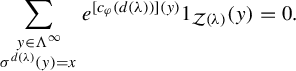 $$ \begin{align*}\sum_{\substack{y \in \Lambda^{\infty} \\ \sigma^{d ({\unicode{x3bb}})} ({y}) = x}} e^{[ c_{\varphi} ({d ({\unicode{x3bb}})}) ] ({y})} 1_{\mathcal{Z} ({\unicode{x3bb}})} ({y}) = 0. \end{align*} $$
It follows that
 $$ \begin{align*} &\int_{\Lambda^{\infty}} ~ {\bigg[{\sum_{\substack{y \in \Lambda^{\infty} \\ \sigma^{d ({\unicode{x3bb}})} ({y}) = x}} e^{[ c_{\varphi} ({d ({\unicode{x3bb}})}) ] ({y})} 1_{\mathcal{Z} ({\unicode{x3bb}})} ({y})}\bigg]} \mathrm{d} {\mu^{\varphi}}({x})\\ &\quad= \int_{\mathcal{Z} ({s ({\unicode{x3bb}})})} ~ {\bigg[{\sum_{\substack{y \in \Lambda^{\infty} \\ \sigma^{d ({\unicode{x3bb}})} ({y}) = x}} e^{[ c_{\varphi} ({d ({\unicode{x3bb}})}) ] ({y})} 1_{\mathcal{Z} ({\unicode{x3bb}})} ({y})}\bigg]} \mathrm{d} {\mu^{\varphi}}({x }). \end{align*} $$
Given an
 $ x \in \mathcal {Z} ({s ({\unicode{x3bb} })}) $
, there exists precisely one
$ x \in \mathcal {Z} ({s ({\unicode{x3bb} })}) $
, there exists precisely one
 $ y \in \mathcal {Z} ({\unicode{x3bb} }) $
such that
$ y \in \mathcal {Z} ({\unicode{x3bb} }) $
such that
 $ \sigma ^{d ({\unicode{x3bb} })} ({y}) = x $
, namely,
$ \sigma ^{d ({\unicode{x3bb} })} ({y}) = x $
, namely,
 $ \unicode{x3bb} x $
. Consequently,
$ \unicode{x3bb} x $
. Consequently,
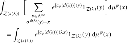 $$ \begin{align*} &\int_{\mathcal{Z} ({s ({\unicode{x3bb}})})} ~ {\bigg[{\sum_{\substack{y \in \Lambda^{\infty}\\ \sigma^{d ({\unicode{x3bb}})} ({y}) = x}}e^{[ c_{\varphi} ({d ({\unicode{x3bb}})}) ] ({y})} 1_{\mathcal{Z} ({\unicode{x3bb}})} ({y})}\bigg]} \mathrm{d} {\mu^{\varphi}}({x})\\ &\quad= \int_{\mathcal{Z} ({s ({\unicode{x3bb}})})} e^{[ c_{\varphi} ({d ({\unicode{x3bb}})}) ] ({\unicode{x3bb} x})} 1_{\mathcal{Z} ({\unicode{x3bb}})} ({y}) ~ \mathrm{d} \mu^{\varphi} ({x}). \end{align*} $$
Therefore,
 $$ \begin{align*}\int_{\mathcal{Z} ({s ({\unicode{x3bb}})})} e^{[ c_{\varphi} ({d ({\unicode{x3bb}})}) ] ({\unicode{x3bb} x})} ~ \mathrm{d} \mu^{\varphi} ({x}) = ({\boldsymbol{\unicode{x3bb}}^{\varphi}})^{d ({\unicode{x3bb}})} \mu^{\varphi} ({\mathcal{Z} ({\unicode{x3bb}})}) \end{align*} $$
and a simple rearrangement of terms yields the proposition.
We list an important positivity property of the measure
 $ \mu ^{\varphi } $
in the event that
$ \mu ^{\varphi } $
in the event that
 $ ({\Lambda ^{\infty },\sigma ,\varphi }) $
satisfies the conditions in Definition 4.2.
$ ({\Lambda ^{\infty },\sigma ,\varphi }) $
satisfies the conditions in Definition 4.2.
Corollary 6.10. Let
 $ \Lambda $
be a
$ \Lambda $
be a
 $ k $
-graph satisfying the standing assumptions of (14). Suppose that
$ k $
-graph satisfying the standing assumptions of (14). Suppose that
 $ ({\Lambda ^{\infty },\sigma ,\varphi }) $
is a
$ ({\Lambda ^{\infty },\sigma ,\varphi }) $
is a
 $ k $
-Ruelle dynamical system that satisfies the conditions of Definition 4.2. Then
$ k $
-Ruelle dynamical system that satisfies the conditions of Definition 4.2. Then
 $ \mu ^{\varphi } ({\mathcal {Z} ({\unicode{x3bb} })})> 0 $
for every
$ \mu ^{\varphi } ({\mathcal {Z} ({\unicode{x3bb} })})> 0 $
for every
 $ \unicode{x3bb} \in \Lambda $
.
$ \unicode{x3bb} \in \Lambda $
.
Proof Suppose by way of contradiction that there exists
 $ \unicode{x3bb} \in \Lambda $
such that
$ \unicode{x3bb} \in \Lambda $
such that
 $ \mu ^{\varphi } ({\mathcal {Z} ({\unicode{x3bb} })}) = 0 $
. By Lemma 6.7, if
$ \mu ^{\varphi } ({\mathcal {Z} ({\unicode{x3bb} })}) = 0 $
. By Lemma 6.7, if
 $ ({1})_{i \in [ k ]} \leq p $
, then
$ ({1})_{i \in [ k ]} \leq p $
, then
 $ \sigma ^{p} $
is positively expansive and exact. But then there exists
$ \sigma ^{p} $
is positively expansive and exact. But then there exists
 $ n \in \mathbb {N} $
such that
$ n \in \mathbb {N} $
such that
 $ \sigma ^{n p} [ \mathcal {Z} ({\unicode{x3bb} }) ] = \Lambda ^{\infty } $
. We now use Proposition 4.2 of [Reference Renault24] again to deduce that
$ \sigma ^{n p} [ \mathcal {Z} ({\unicode{x3bb} }) ] = \Lambda ^{\infty } $
. We now use Proposition 4.2 of [Reference Renault24] again to deduce that
 $$ \begin{align*}\mu^{\varphi} ({\Lambda^{\infty}}) = \mu^{\varphi} ({\sigma^{n p} [ \mathcal{Z} ({\unicode{x3bb}}) ]}) = \mu^{\varphi} ({\mathcal{Z} ({\unicode{x3bb}})}) = 0. \end{align*} $$
Since
 $ \mu ^{\varphi } ({\Lambda ^{\infty }}) = 1 $
, this gives us a contradiction.
$ \mu ^{\varphi } ({\Lambda ^{\infty }}) = 1 $
, this gives us a contradiction.
Recall that if
 $ \Lambda $
is a
$ \Lambda $
is a
 $ k $
-graph and
$ k $
-graph and
 $ H $
is an abelian group, a map
$ H $
is an abelian group, a map
 $ h: \Lambda \to H $
is called a categorical
$ h: \Lambda \to H $
is called a categorical
 $ 1 $
-cocycle if
$ 1 $
-cocycle if
 $ h ({\unicode{x3bb} \mu }) = h ({\unicode{x3bb} }) + h ({\mu }) $
whenever
$ h ({\unicode{x3bb} \mu }) = h ({\unicode{x3bb} }) + h ({\mu }) $
whenever
 $ ({\unicode{x3bb} ,\mu }) $
is composable. In the case when
$ ({\unicode{x3bb} ,\mu }) $
is composable. In the case when
 $ H = \mathbb {R} $
and the image of
$ H = \mathbb {R} $
and the image of
 $ h $
lies entirely inside the non-negative real numbers,
$ h $
lies entirely inside the non-negative real numbers,
 $ h $
was called an ‘
$ h $
was called an ‘
 $ \mathbb {R}^{+} $
-functor’ in [Reference Farsi, Gillaspy, Larsen and Packer12].
$ \mathbb {R}^{+} $
-functor’ in [Reference Farsi, Gillaspy, Larsen and Packer12].
Next, observe that, if
 $ h $
is a categorical
$ h $
is a categorical
 $ 1 $
-cocycle taking values in
$ 1 $
-cocycle taking values in
 $ \mathbb {R} $
, then a routine calculation shows that the
$ \mathbb {R} $
, then a routine calculation shows that the
 $ k $
-tuple of functions
$ k $
-tuple of functions
 $ \varphi ^{h,\theta } := ({\varphi ^{h,\theta }_{i}})_{i \in [ k ]} $
, where
$ \varphi ^{h,\theta } := ({\varphi ^{h,\theta }_{i}})_{i \in [ k ]} $
, where
 $ \varphi ^{h,\theta }_{i}: \Lambda ^{\infty } \to \mathbb {R} $
is defined for all
$ \varphi ^{h,\theta }_{i}: \Lambda ^{\infty } \to \mathbb {R} $
is defined for all
 $ i \in [ k ] $
and
$ i \in [ k ] $
and
 $ x \in \Lambda ^{\infty } $
by
$ x \in \Lambda ^{\infty } $
by
 $$ \begin{align} \varphi^{h,\theta}_{i} ({x}) = - \theta h ({x ({0,\mathbf{e}_{i}})}), \end{align} $$
satisfies the cocycle condition and therefore determines a groupoid
 $ 1 $
-cocycle on
$ 1 $
-cocycle on
 $ \mathcal {G} ({\Lambda ^{\infty },\sigma }) $
taking values in
$ \mathcal {G} ({\Lambda ^{\infty },\sigma }) $
taking values in
 $ \mathbb {R} $
by Lemma 3.12; we will call this cocycle
$ \mathbb {R} $
by Lemma 3.12; we will call this cocycle
 $ c_{\varphi ^{h,\theta }} $
. Hence,
$ c_{\varphi ^{h,\theta }} $
. Hence,
 $ ({\Lambda ^{\infty },\sigma ,c_{\varphi ^{h,\theta }}}) $
is a
$ ({\Lambda ^{\infty },\sigma ,c_{\varphi ^{h,\theta }}}) $
is a
 $ k $
-Ruelle dynamical system.
$ k $
-Ruelle dynamical system.
Example 5.4 has shown that an automorphism group on a
 $ C^{\ast } $
-algebra coming from
$ C^{\ast } $
-algebra coming from
 $ ({X,\sigma ,\varphi }) $
need not have a KMS state. However, by using Corollary 5.8 and other results, we can construct a new cocycle from
$ ({X,\sigma ,\varphi }) $
need not have a KMS state. However, by using Corollary 5.8 and other results, we can construct a new cocycle from
 $ \varphi $
giving rise to a different dynamics for which a KMS state does exist. The following theorem was first proved in a different way in Proposition 4.4 in [Reference Farsi, Gillaspy, Larsen and Packer12].
$ \varphi $
giving rise to a different dynamics for which a KMS state does exist. The following theorem was first proved in a different way in Proposition 4.4 in [Reference Farsi, Gillaspy, Larsen and Packer12].
Theorem 6.11. [Reference Farsi, Gillaspy, Larsen and Packer12]
Let
 $ \Lambda $
be a
$ \Lambda $
be a
 $ k $
-graph satisfying the standing assumptions of (14). Let
$ k $
-graph satisfying the standing assumptions of (14). Let
 $ h: \Lambda \to \mathbb {R} $
be a non-negative categorical
$ h: \Lambda \to \mathbb {R} $
be a non-negative categorical
 $ 1 $
-cocycle and let
$ 1 $
-cocycle and let
 $ \theta $
be a positive real number. Let
$ \theta $
be a positive real number. Let
 $ \varphi ^{h,\theta } = ({\varphi ^{h,\theta }_i})_{i \in [ k ]} $
be as defined in equation (15). Then
$ \varphi ^{h,\theta } = ({\varphi ^{h,\theta }_i})_{i \in [ k ]} $
be as defined in equation (15). Then
 $ ({\Lambda ^{\infty },\sigma ,\varphi ^{h,\theta }}) $
is a
$ ({\Lambda ^{\infty },\sigma ,\varphi ^{h,\theta }}) $
is a
 $ k $
-Ruelle dynamical system that satisfies the conditions in Definition 4.2 and, for each
$ k $
-Ruelle dynamical system that satisfies the conditions in Definition 4.2 and, for each
 $ \beta \in \mathbb {R}\setminus \{0\} $
, so does
$ \beta \in \mathbb {R}\setminus \{0\} $
, so does
 $$ \begin{align*}\bigg({\Lambda^{\infty}},{\sigma},{\bigg({\frac{1}{\beta} ({\ln ({\unicode{x3bb}^{\varphi^{h,\theta}}_{i}}) - \varphi^{h,\theta}_{i}})}\bigg)_{i \in [ k ]}}\bigg). \end{align*} $$
The associated generalized state
 $ \omega $
on
$ \omega $
on
 $ C^{\ast }_{\textrm {r}} ({\mathcal {G} ({\Lambda ^{\infty },\sigma })}) \cong C^{\ast } ({\Lambda }) $
uniquely determined by
$ C^{\ast }_{\textrm {r}} ({\mathcal {G} ({\Lambda ^{\infty },\sigma })}) \cong C^{\ast } ({\Lambda }) $
uniquely determined by
 $$ \begin{align*}\text{ for all } f \in \operatorname{C_{c}} ({\mathcal{G} ({\Lambda^{\infty},\sigma})}): \omega ({f}) = \int_{\Lambda^{\infty}} f ({x,0,x}) ~ \mathrm{d} \mu^{\varphi^{h,\theta}}(x) \end{align*} $$
is a
 $ \operatorname {KMS}_{\beta } $
state for the dynamics determined by the cocycle
$ \operatorname {KMS}_{\beta } $
state for the dynamics determined by the cocycle
 $ \varsigma $
given by
$ \varsigma $
given by
 $$ \begin{align*}\varsigma := \bigg({\frac{1}{\beta} ({\ln ({\unicode{x3bb}^{\varphi^{h,\theta}}_{i}}) - \varphi^{h,\theta}_{i}})}\bigg)_{i \in [ k ]}; \end{align*} $$
moreover,
 $ \mu ^{\varsigma } = \mu ^{\varphi ^{h,\theta }} $
.
$ \mu ^{\varsigma } = \mu ^{\varphi ^{h,\theta }} $
.
Proof Fix an arbitrary
 $ n \in \mathbb {N}^{k} $
. We will first prove that the function
$ n \in \mathbb {N}^{k} $
. We will first prove that the function
 $ f: \Lambda ^{\infty } \to \mathbb {R} $
defined by, for all
$ f: \Lambda ^{\infty } \to \mathbb {R} $
defined by, for all
 $x \in \Lambda ^{\infty }$
,
$x \in \Lambda ^{\infty }$
,
 $$ \begin{align*}f ({x}) := h ({x ({0,n})}) \end{align*} $$
is Hölder-continuous with respect to
 $ \rho _{\Lambda } $
. As
$ \rho _{\Lambda } $
. As
 $ \Lambda ^{n} $
is finite,
$ \Lambda ^{n} $
is finite,
 $ h $
clearly achieves both a minimum value
$ h $
clearly achieves both a minimum value
 $ m $
and a maximum value
$ m $
and a maximum value
 $ M $
on
$ M $
on
 $ \Lambda ^{n} $
. Choose
$ \Lambda ^{n} $
. Choose
 $ N \in \mathbb {N} $
such that
$ N \in \mathbb {N} $
such that
 $ n \leq N p $
with
$ n \leq N p $
with
 $ ({1})_{i \in [ k ]} \leq p $
. For
$ ({1})_{i \in [ k ]} \leq p $
. For
 $ x,y \in \Lambda ^{\infty } $
such that
$ x,y \in \Lambda ^{\infty } $
such that
 $ \rho _{\Lambda } ({x,y}) < {1}/{2^{N}} $
, for all
$ \rho _{\Lambda } ({x,y}) < {1}/{2^{N}} $
, for all
 $ j \in [ N ] $
,
$ j \in [ N ] $
,
 $$ \begin{align*}x ({j p,({j + 1}) p}) = y ({j p,({j + 1}) p}), \end{align*} $$
so
 $ x ({0,N p}) = y ({0,N p}) $
, which yields
$ x ({0,N p}) = y ({0,N p}) $
, which yields
 $ x ({0,n}) = y ({0,n}) $
by the factorization property. Consequently, for all
$ x ({0,n}) = y ({0,n}) $
by the factorization property. Consequently, for all
 $x,y \in \Lambda ^{\infty }$
,
$x,y \in \Lambda ^{\infty }$
,
 $$ \begin{align*}\lvert f ({x}) - f ({y}) \rvert = \lvert h ({x ({0,n})}) - h ({y ({0,n})}) \rvert \leq N ({M - m}) \rho_{\Lambda} ({x,y}). \end{align*} $$
As
 $ n \in \mathbb {N}^{k} $
is arbitrary, it follows that
$ n \in \mathbb {N}^{k} $
is arbitrary, it follows that
 $ \varphi ^{h,\theta }_{i} $
is Hölder-continuous with respect to
$ \varphi ^{h,\theta }_{i} $
is Hölder-continuous with respect to
 $ \rho _{\Lambda } $
for each
$ \rho _{\Lambda } $
for each
 $ i \in [ k ] $
.
$ i \in [ k ] $
.
A straightforward calculation demonstrates that
 $ c_{\varphi ^{h,\theta }} ({p}) $
is Hölder-continuous with respect to
$ c_{\varphi ^{h,\theta }} ({p}) $
is Hölder-continuous with respect to
 $ \rho _{\Lambda } $
; therefore, by applying Theorem 6.8, we conclude that
$ \rho _{\Lambda } $
; therefore, by applying Theorem 6.8, we conclude that
 $ ({\Lambda ^{\infty },\sigma ,\varphi ^{h,\theta }}) $
satisfies the conditions in Definition 4.2.
$ ({\Lambda ^{\infty },\sigma ,\varphi ^{h,\theta }}) $
satisfies the conditions in Definition 4.2.
Applying Theorem 6.8, we conclude that
 $ ({\Lambda ^{\infty },\sigma ,\varphi ^{h,\theta }}) $
satisfies the conditions in Definition 4.2.
$ ({\Lambda ^{\infty },\sigma ,\varphi ^{h,\theta }}) $
satisfies the conditions in Definition 4.2.
It now follows from Corollary 5.8 that
 $$ \begin{align*}\bigg({\Lambda^{\infty}},{\sigma},{\bigg({\frac{1}{\beta} ({\ln ({\unicode{x3bb}^{\varphi^{h,\theta}}_{i}}) - \varphi^{h,\theta}_{i}})}\bigg)_{i \in [ k ]}}\bigg) \end{align*} $$
also satisfies the conditions in Definition 4.2, with
 $ \mu ^{\varsigma } = \mu ^{\varphi ^{h,\theta }}$
, by Corollary 5.8. By Proposition 5.6, the state
$ \mu ^{\varsigma } = \mu ^{\varphi ^{h,\theta }}$
, by Corollary 5.8. By Proposition 5.6, the state
 $ \omega $
on
$ \omega $
on
 $ C^{\ast } ({\mathcal {G} ({\Lambda ^{\infty },\sigma })}) \cong C^{\ast } ({\Lambda }) $
that is uniquely determined by, for all
$ C^{\ast } ({\mathcal {G} ({\Lambda ^{\infty },\sigma })}) \cong C^{\ast } ({\Lambda }) $
that is uniquely determined by, for all
 $f \in \operatorname {C_{c}} ({\mathcal {G} ({\Lambda ^{\infty },\sigma })})$
,
$f \in \operatorname {C_{c}} ({\mathcal {G} ({\Lambda ^{\infty },\sigma })})$
,
 $$ \begin{align*}\omega ({f}) = \int_{\Lambda^{\infty}} f ({x,0,x}) ~ \mathrm{d} \mu^{\varphi^{h,\theta}}(x), \end{align*} $$
with notation as in Proposition 6.9, is a
 $ \operatorname {KMS}_{\beta } $
state for the generalized gauge dynamics of this particular dynamical system.
$ \operatorname {KMS}_{\beta } $
state for the generalized gauge dynamics of this particular dynamical system.
The following corollary gives more information about the eigenmeasure
 $ \mu ^{\varphi ^{h,\theta }} $
and relates it to the eigenvalues of the Ruelle–Perron–Frobenius operator.
$ \mu ^{\varphi ^{h,\theta }} $
and relates it to the eigenvalues of the Ruelle–Perron–Frobenius operator.
Corollary 6.12. Let
 $ \Lambda $
be a
$ \Lambda $
be a
 $ k $
-graph satisfying the standing assumptions of (14) and let
$ k $
-graph satisfying the standing assumptions of (14) and let
 $ h: \Lambda \to \mathbb {R}_{\geq 0} $
,
$ h: \Lambda \to \mathbb {R}_{\geq 0} $
,
 $ \theta \in \mathbb {R} \setminus \{0\} $
, and
$ \theta \in \mathbb {R} \setminus \{0\} $
, and
 $ \varphi ^{h,\theta } $
be as in Theorem 6.11; let
$ \varphi ^{h,\theta } $
be as in Theorem 6.11; let
 $ c_{\varphi ^{h,\theta }} $
denote the associated cocycle. Then, for all
$ c_{\varphi ^{h,\theta }} $
denote the associated cocycle. Then, for all
 $ \unicode{x3bb} \in \Lambda $
,
$ \unicode{x3bb} \in \Lambda $
,
 $$ \begin{align*}\mu^{\varphi^{h,\theta}} ({\mathcal{Z} ({\unicode{x3bb}})}) = ({\boldsymbol{\unicode{x3bb}}^{\varphi^{h,\theta}}})^{- d ({\unicode{x3bb}})} e^{- \theta h ({\unicode{x3bb}})} \mu^{\varphi^{h,\theta}} ({\mathcal{Z} ({s ({\unicode{x3bb}})})}), \end{align*} $$
where
 $ \varphi ^{h,\theta } $
is the
$ \varphi ^{h,\theta } $
is the
 $ k $
-tuple of elements of
$ k $
-tuple of elements of
 $ \operatorname {C} ({\Lambda ^{\infty },\mathbb {R}}) $
that is defined for all
$ \operatorname {C} ({\Lambda ^{\infty },\mathbb {R}}) $
that is defined for all
 $ i \in [ k ] $
and
$ i \in [ k ] $
and
 $ x \in \Lambda ^{\infty } $
by
$ x \in \Lambda ^{\infty } $
by
 $$ \begin{align*}\varphi^{h,\theta}_{i} ({x}) := - \theta h ({x ({0,\mathbf{e}_{i}})}). \end{align*} $$
Proof We already know from Theorem 7.9 that for all
 $ n \in \mathbb {N}^{k} $
and
$ n \in \mathbb {N}^{k} $
and
 $ x \in \Lambda ^{\infty } $
,
$ x \in \Lambda ^{\infty } $
,
 $$ \begin{align*}c_{\varphi^{h,\theta}} ({n}) = - \theta h ({x ({0,n})}). \end{align*} $$
Hence, for every
 $ \unicode{x3bb} \in \Lambda $
, if
$ \unicode{x3bb} \in \Lambda $
, if
 $ x \in \mathcal {Z} ({s ({\unicode{x3bb} })}) $
, we have
$ x \in \mathcal {Z} ({s ({\unicode{x3bb} })}) $
, we have
 $$ \begin{align*}[ c_{\varphi^{h,\theta}} ({d ({\unicode{x3bb}})}) ] ({\unicode{x3bb} x}) = - \theta h ({({\unicode{x3bb} x}) ({0,d ({\unicode{x3bb}})})}) = - \theta h ({\unicode{x3bb}}). \end{align*} $$
Consequently, by Proposition 6.9, for all
 $ \unicode{x3bb} \in \Lambda $
,
$ \unicode{x3bb} \in \Lambda $
,
 $$ \begin{align*} \mu^{\varphi^{h,\theta}} ({\mathcal{Z} ({\unicode{x3bb}})}) & = ({\boldsymbol{\unicode{x3bb}}^{\varphi^{h,\theta}}})^{- d ({\unicode{x3bb}})} \int_{\mathcal{Z} ({s ({\unicode{x3bb}})})} e^{[ c_{\varphi^{h,\theta}} ({d ({\unicode{x3bb}})}) ] ({\unicode{x3bb} x})} ~ \mathrm{d} \mu^{\varphi^{h,\theta}} ({x}) \\ & = ({\boldsymbol{\unicode{x3bb}}^{\varphi^{h,\theta}}})^{- d ({\unicode{x3bb}})} \int_{\mathcal{Z} ({s ({\unicode{x3bb}})})} e^{- \theta h ({\unicode{x3bb}})} ~ \mathrm{d} \mu^{\varphi^{h,\theta}} ({x}) \\ & = ({\boldsymbol{\unicode{x3bb}}^{\varphi^{h,\theta}}})^{- d ({\unicode{x3bb}})} e^{- \theta h ({\unicode{x3bb}})} \int_{\mathcal{Z} ({s ({\unicode{x3bb}})})} 1 ~ \mathrm{d} \mu^{\varphi^{h,\theta}} ({x}) \\ & = ({\boldsymbol{\unicode{x3bb}}^{\varphi^{h,\theta}}})^{- d ({\unicode{x3bb}})} e^{- \theta h ({\unicode{x3bb}})} \mu^{\varphi^{h,\theta}} ({\mathcal{Z} ({s ({\unicode{x3bb}})})}). \end{align*} $$
The corollary is therefore proven.
Acknowledgments
This work was partially supported by Simons Foundation Collaboration grants #523991 (C.F.), #353626 (A.K.), and #316981 (J.P.). C.F. thanks the sabbatical program at the University of Colorado Boulder for support. A.K. would like to thank C.F and J.P. for their kind hospitality on a recent visit to Boulder. The authors also thank the referee for helpful suggestions.


 Open access