


1 Introduction
Self-similar measures in ${\mathbb {R}}$
are perhaps the simplest examples of measures which exhibit complex local structure. These measures are associated with finite sets of similarity maps in
${\mathbb {R}}$
are perhaps the simplest examples of measures which exhibit complex local structure. These measures are associated with finite sets of similarity maps in ${\mathbb {R}}$
. To be precise, by an iterated function system of similarities (IFS), we mean a finite set of maps
${\mathbb {R}}$
. To be precise, by an iterated function system of similarities (IFS), we mean a finite set of maps $\{S_{i}\}_{i\in \mathcal {I}}$
where each
$\{S_{i}\}_{i\in \mathcal {I}}$
where each $S_{i}(x)=r_{i} x+d_{i}$
and
$S_{i}(x)=r_{i} x+d_{i}$
and $0<|r_{i}|<1$
. The attractor, or self-similar set, of this system is the unique compact set K satisfying
$0<|r_{i}|<1$
. The attractor, or self-similar set, of this system is the unique compact set K satisfying $\bigcup _{i\in \mathcal {I}}S_{i}(K)=K$
. Given a probability vector
$\bigcup _{i\in \mathcal {I}}S_{i}(K)=K$
. Given a probability vector $\boldsymbol {p}=(p_{i})_{i\in \mathcal {I}}$
where each
$\boldsymbol {p}=(p_{i})_{i\in \mathcal {I}}$
where each $p_{i}>0$
and
$p_{i}>0$
and $\sum _{i} p_{i}=1$
, the associated self-similar measure is the unique Borel probability measure satisfying
$\sum _{i} p_{i}=1$
, the associated self-similar measure is the unique Borel probability measure satisfying
 $$ \begin{align*} {\mu_{\boldsymbol{p}}}(E)=\sum_{i\in\mathcal{I}}p_{i}{\mu_{\boldsymbol{p}}}\circ S_{i}^{-1}(E) \end{align*} $$
for any Borel set $E\subseteq {\mathbb {R}}$
. For a more through discussion of the background and basic properties of self-similar sets and measures, we refer the reader to Falconer’s book [Reference Falconer6].
$E\subseteq {\mathbb {R}}$
. For a more through discussion of the background and basic properties of self-similar sets and measures, we refer the reader to Falconer’s book [Reference Falconer6].
To understand the general structure of the measure ${\mu _{\boldsymbol {p}}}$
or the self-similar set K, one often considers basic dimensional quantities such as the Hausdorff dimension
${\mu _{\boldsymbol {p}}}$
or the self-similar set K, one often considers basic dimensional quantities such as the Hausdorff dimension $\operatorname {dim}_{\mathrm {H}} K$
and analogous statements for measures, or other notions of dimension. Computing these values can be highly non-trivial for general iterated function systems of similarities and there is significant literature on this matter (see, for example, [Reference Bandt and Graf2, Reference Feng and Hu12, Reference Fraser, Henderson, Olson and Robinson16, Reference Hochman23, Reference Jordan and Rapaport26, Reference Lau and Ngai29, Reference Ngai and Wang32, Reference Schief36]). In this paper, we focus on a more fine-grained notion of dimension known as the local dimension. Given a point
$\operatorname {dim}_{\mathrm {H}} K$
and analogous statements for measures, or other notions of dimension. Computing these values can be highly non-trivial for general iterated function systems of similarities and there is significant literature on this matter (see, for example, [Reference Bandt and Graf2, Reference Feng and Hu12, Reference Fraser, Henderson, Olson and Robinson16, Reference Hochman23, Reference Jordan and Rapaport26, Reference Lau and Ngai29, Reference Ngai and Wang32, Reference Schief36]). In this paper, we focus on a more fine-grained notion of dimension known as the local dimension. Given a point $x\in K=\operatorname {\mathrm {supp}}{\mu _{\boldsymbol {p}}}$
, the local dimension is given by
$x\in K=\operatorname {\mathrm {supp}}{\mu _{\boldsymbol {p}}}$
, the local dimension is given by
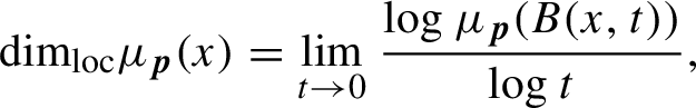 $$ \begin{align*} {\dim_{\operatorname{\mathrm{loc}}}}{\mu_{\boldsymbol{p}}}(x)=\lim_{t\to 0}\frac{\log {\mu_{\boldsymbol{p}}}(B(x,t))}{\log t}, \end{align*} $$
when the limit exists. From the perspective of multifractal analysis, one is interested in determining geometric properties of the sets $K(\alpha ):= \{x\in K:{\dim _{\operatorname {\mathrm {loc}}}}{\mu _{\boldsymbol {p}}}(x)=\alpha \}$
. However, the
$K(\alpha ):= \{x\in K:{\dim _{\operatorname {\mathrm {loc}}}}{\mu _{\boldsymbol {p}}}(x)=\alpha \}$
. However, the $L^{q}$
-spectrum of
$L^{q}$
-spectrum of ${\mu _{\boldsymbol {p}}}$
is given by
${\mu _{\boldsymbol {p}}}$
is given by
 $$ \begin{align*} \tau({\mu_{\boldsymbol{p}}},q)=\tau(q):= \liminf_{t\to 0}\frac{\log \sup\sum_{i}{\mu_{\boldsymbol{p}}}(B(x_{i},t))^{q}}{\log t} \end{align*} $$
for each $q\in {\mathbb {R}}$
, where the supremum is over disjoint families of closed balls with centres
$q\in {\mathbb {R}}$
, where the supremum is over disjoint families of closed balls with centres $x_{i}\in K$
.
$x_{i}\in K$
.
An important objective of multifractal analysis is to understand the relationship between the $L^{q}$
-spectrum of the measure
$L^{q}$
-spectrum of the measure ${\mu _{\boldsymbol {p}}}$
and the dimension spectrum
${\mu _{\boldsymbol {p}}}$
and the dimension spectrum $\operatorname {dim}_{\mathrm {H}} K(\alpha )$
. A heuristic relationship between
$\operatorname {dim}_{\mathrm {H}} K(\alpha )$
. A heuristic relationship between $\tau (q)$
and
$\tau (q)$
and $\operatorname {dim}_{\mathrm {H}} K(\alpha )$
, known as the multifractal formalism, was introduced by Halsey et al. [Reference Halsey, Jensen, Kadanoff, Procaccia and Shraiman17]. The multifractal formalism states, roughly speaking, that the dimension spectrum can be computed as the concave conjugate of
$\operatorname {dim}_{\mathrm {H}} K(\alpha )$
, known as the multifractal formalism, was introduced by Halsey et al. [Reference Halsey, Jensen, Kadanoff, Procaccia and Shraiman17]. The multifractal formalism states, roughly speaking, that the dimension spectrum can be computed as the concave conjugate of $\tau (q)$
, that is,
$\tau (q)$
, that is,
 $$ \begin{align*} \operatorname{dim}_{\mathrm{H}} K(\alpha) =\tau^{*}(\alpha):= \inf_{q\in{\mathbb{R}}}\{q\alpha-\tau(q)\} \end{align*} $$
for any $\alpha $
in the domain of
$\alpha $
in the domain of $\tau ^{*}(\alpha )$
; see Definition 4.2 for a complete definition in our setting. This concave conjugate relationship has been studied by many authors (see, for example, [Reference Cawley and Mauldin3, Reference Feng7, Reference Feng10, Reference Feng and Lau13, Reference Feng, Lau and Wang14, Reference Halsey, Jensen, Kadanoff, Procaccia and Shraiman17, Reference Lau, Bandt, Graf and Zähle27, Reference Lau and Ngai28, Reference Patzschke33, Reference Pesin and Weiss34, Reference Shmerkin38]). As a particularly elegant example, it has been verified in general for iterated function systems satisfying the strong separation condition (
$\tau ^{*}(\alpha )$
; see Definition 4.2 for a complete definition in our setting. This concave conjugate relationship has been studied by many authors (see, for example, [Reference Cawley and Mauldin3, Reference Feng7, Reference Feng10, Reference Feng and Lau13, Reference Feng, Lau and Wang14, Reference Halsey, Jensen, Kadanoff, Procaccia and Shraiman17, Reference Lau, Bandt, Graf and Zähle27, Reference Lau and Ngai28, Reference Patzschke33, Reference Pesin and Weiss34, Reference Shmerkin38]). As a particularly elegant example, it has been verified in general for iterated function systems satisfying the strong separation condition ( $S_{i}(K)\cap S_{j}(K)\neq \emptyset $
if and only if
$S_{i}(K)\cap S_{j}(K)\neq \emptyset $
if and only if $i=j$
) [Reference Cawley and Mauldin3]. This separation requirement has been relaxed to the open set condition [Reference Hutchinson25] and the concave conjugate relationship has been verified [Reference Arbeiter and Patzschke1, Reference Patzschke33, Reference Pesin and Weiss34]. In both cases,
$i=j$
) [Reference Cawley and Mauldin3]. This separation requirement has been relaxed to the open set condition [Reference Hutchinson25] and the concave conjugate relationship has been verified [Reference Arbeiter and Patzschke1, Reference Patzschke33, Reference Pesin and Weiss34]. In both cases, $\tau (q)$
is differentiable for all
$\tau (q)$
is differentiable for all $q\in {\mathbb {R}}$
and is determined uniquely by the implicit formula
$q\in {\mathbb {R}}$
and is determined uniquely by the implicit formula $\sum _{i\in \mathcal {I}}p_{i}^{q} r_{i}^{-\tau (q)}=1$
.
$\sum _{i\in \mathcal {I}}p_{i}^{q} r_{i}^{-\tau (q)}=1$
.
However, when the open set condition fails, outside specialized analysis of some families of examples (for example, Bernoulli convolutions associated with the unique positive root of the polynomial $x^{k}-x^{k-1}-\cdots -x-1$
[Reference Feng9]), there has been much less progress on verifying the multifractal formalism at all
$x^{k}-x^{k-1}-\cdots -x-1$
[Reference Feng9]), there has been much less progress on verifying the multifractal formalism at all $q\in {\mathbb {R}}$
. For
$q\in {\mathbb {R}}$
. For $q\geq 0$
, the function
$q\geq 0$
, the function $x\mapsto x^{q}$
is non-decreasing so the summation in the definition of
$x\mapsto x^{q}$
is non-decreasing so the summation in the definition of $\tau (q)$
is dominated by closed balls with large measure. However, for
$\tau (q)$
is dominated by closed balls with large measure. However, for $q<0$
, the summation is dominated by closed balls of small measure. Generally speaking, understanding the multifractal analysis of measures when
$q<0$
, the summation is dominated by closed balls of small measure. Generally speaking, understanding the multifractal analysis of measures when $q<0$
is substantially more challenging than the case
$q<0$
is substantially more challenging than the case $q\geq 0$
. Gaining more information about this case is our focus in this document.
$q\geq 0$
. Gaining more information about this case is our focus in this document.
1.1 The weak separation condition
Notably, neither the strong separation condition nor the open set condition allows for the existence of exact overlaps. We introduce some notation: let $\mathcal {I}^{*}$
denote the set of all finite words on
$\mathcal {I}^{*}$
denote the set of all finite words on $\mathcal {I}$
. For
$\mathcal {I}$
. For $\sigma =(i_{1},\ldots ,i_{n})\in \mathcal {I}^{*}$
, write
$\sigma =(i_{1},\ldots ,i_{n})\in \mathcal {I}^{*}$
, write $S_{\sigma }=S_{i_{1}}\circ \cdots \circ S_{i_{n}}$
,
$S_{\sigma }=S_{i_{1}}\circ \cdots \circ S_{i_{n}}$
, $r_{\sigma }=r_{i_{1}}\cdots r_{i_{n}}$
and, if
$r_{\sigma }=r_{i_{1}}\cdots r_{i_{n}}$
and, if $n\geq 1$
,
$n\geq 1$
, $\sigma ^{-}=(i_{1},\ldots ,i_{n-1})$
. By exact overlaps, we mean the existence of words
$\sigma ^{-}=(i_{1},\ldots ,i_{n-1})$
. By exact overlaps, we mean the existence of words $\sigma \neq \tau \in \mathcal {I}^{*}$
such that
$\sigma \neq \tau \in \mathcal {I}^{*}$
such that $S_{\sigma }=S_{\tau }$
. To study examples allowing exact overlaps while still maintaining separation of non-overlapping words, Lau and Ngai introduced the weak separation condition and studied basic conditions under which the multifractal formalism holds [Reference Lau and Ngai28]. For any
$S_{\sigma }=S_{\tau }$
. To study examples allowing exact overlaps while still maintaining separation of non-overlapping words, Lau and Ngai introduced the weak separation condition and studied basic conditions under which the multifractal formalism holds [Reference Lau and Ngai28]. For any $t>0$
and Borel set
$t>0$
and Borel set $E\subseteq {\mathbb {R}}$
, define
$E\subseteq {\mathbb {R}}$
, define
 $$ \begin{align*} \Lambda_{t}(E) = \{\sigma\in\mathcal{I}^{*}:r_{\sigma}< t\leq r_{\sigma^{-}},S_{\sigma}(K)\cap E\neq\emptyset\}. \end{align*} $$
Then the weak separation condition is equivalent to requiring that
 $$ \begin{align} \sup_{x\in{\mathbb{R}},t>0}\#\{S_{\sigma}:\sigma\in\Lambda_{t}(U(x,t))\}<\infty, \end{align} $$
where $\# X$
denotes the cardinality of a set X and
$\# X$
denotes the cardinality of a set X and $U(x,t)$
is the open ball about x with radius t. Note that the definition only considers functions
$U(x,t)$
is the open ball about x with radius t. Note that the definition only considers functions $S_{\sigma }$
rather than the words
$S_{\sigma }$
rather than the words $\sigma $
so as to allow exact overlaps. To see an equivalent formulation with respect to exact overlaps or the equivalence with the original definition of Lau and Ngai, see [Reference Zerner40, Theorem 1].
$\sigma $
so as to allow exact overlaps. To see an equivalent formulation with respect to exact overlaps or the equivalence with the original definition of Lau and Ngai, see [Reference Zerner40, Theorem 1].
Under the weak separation condition, verification of the multifractal formalism is subtle. One of the earliest examples of exceptional behaviour is with respect to self-similar measures of the system of Bernoulli convolutions $\{x\mapsto \rho x,x\mapsto \rho x+(1-\rho )\}$
, where the contraction ratio
$\{x\mapsto \rho x,x\mapsto \rho x+(1-\rho )\}$
, where the contraction ratio $\rho $
is the reciprocal of the golden mean. In this case, the
$\rho $
is the reciprocal of the golden mean. In this case, the $L^{q}$
-spectrum
$L^{q}$
-spectrum $\tau (q)$
has a phase transition, or a point where
$\tau (q)$
has a phase transition, or a point where $\tau (q)$
is not differentiable. Nevertheless, the multifractal formalism still holds and
$\tau (q)$
is not differentiable. Nevertheless, the multifractal formalism still holds and $\tau (q)$
is analytic for other values of q [Reference Feng9]. Another example of exceptional behaviour is the
$\tau (q)$
is analytic for other values of q [Reference Feng9]. Another example of exceptional behaviour is the $3$
-fold convolution of the uniform Cantor measure. In this case, it was observed that the set of attainable local dimensions is not an interval and the multifractal formalism fails [Reference Hu and Lau24]. The problem here is, in some sense, that the measure
$3$
-fold convolution of the uniform Cantor measure. In this case, it was observed that the set of attainable local dimensions is not an interval and the multifractal formalism fails [Reference Hu and Lau24]. The problem here is, in some sense, that the measure ${\mu _{\boldsymbol {p}}}$
is too small at certain points in K. This measure, and other related measures, were studied in detail [Reference Feng, Lau and Wang14, Reference Hare, Hare and Shen21, Reference Lau and Wang31, Reference Shmerkin38] and a modified multifractal formalism was proven therein. In these cases, the failure occurs at some point
${\mu _{\boldsymbol {p}}}$
is too small at certain points in K. This measure, and other related measures, were studied in detail [Reference Feng, Lau and Wang14, Reference Hare, Hare and Shen21, Reference Lau and Wang31, Reference Shmerkin38] and a modified multifractal formalism was proven therein. In these cases, the failure occurs at some point $q<0$
.
$q<0$
.
In an important paper, Feng and Lau [Reference Feng and Lau13] obtain deep results about the multifractal formalism under the weak separation condition. Using a subtle Moran construction [Reference Feng, Lau and Wu15], they prove that the multifractal formalism holds for any value $q\geq 0$
, and for
$q\geq 0$
, and for $q<0$
, they give a modified multifractal formalism by considering suitable restrictions to an open ball
$q<0$
, they give a modified multifractal formalism by considering suitable restrictions to an open ball $U_{0}$
which attains the supremum in the definition of the weak separation condition of equation (1.1). Unfortunately, this result does not directly give information on the validity of the multifractal formalism for values
$U_{0}$
which attains the supremum in the definition of the weak separation condition of equation (1.1). Unfortunately, this result does not directly give information on the validity of the multifractal formalism for values $q<0$
. In some sense, the restriction avoids the breakdown of the multifractal formalism by avoiding points in K where the measure is too small.
$q<0$
. In some sense, the restriction avoids the breakdown of the multifractal formalism by avoiding points in K where the measure is too small.
To extend this perspective, we develop some new ideas. Even in regions where the overlap is not dense (that is, away from any maximal open ball $U_{0}$
), through a general graph construction, we will show that the measure may be ‘combinatorially linked’ to regions with high density where the multifractal formalism holds. For example, consider the IFS given by the maps
$U_{0}$
), through a general graph construction, we will show that the measure may be ‘combinatorially linked’ to regions with high density where the multifractal formalism holds. For example, consider the IFS given by the maps
 $$ \begin{align} S_{1}(x)&=\rho x \quad S_{2}(x)=r x+\rho(1-r) \quad S_{3}(x)=r x+1-r, \end{align} $$
where $\rho>0$
,
$\rho>0$
, $r>0$
satisfy
$r>0$
satisfy $\rho +2r-\rho r\leq 1$
. This IFS was first studied by Lau and Wang [Reference Lau and Wang30] and satisfies the weak separation condition. In §5.3.3, we show that the maximal open sets
$\rho +2r-\rho r\leq 1$
. This IFS was first studied by Lau and Wang [Reference Lau and Wang30] and satisfies the weak separation condition. In §5.3.3, we show that the maximal open sets $U_{0}$
can never contain the point
$U_{0}$
can never contain the point $1$
in the self-similar set, which is a phenomenon similar to the situation of the Cantor convolution. Despite this, we can prove (as a consequence of our more general results) that the multifractal formalism still holds for the measure
$1$
in the self-similar set, which is a phenomenon similar to the situation of the Cantor convolution. Despite this, we can prove (as a consequence of our more general results) that the multifractal formalism still holds for the measure ${\mu _{\boldsymbol {p}}}$
, without restriction to a subset and with any probabilities. Our main goal in this paper is to provide a new, natural perspective for understanding the failure of the multifractal formalism, and to provide combinatorial conditions under which the multifractal formalism holds or in which one might suspect that it fails.
${\mu _{\boldsymbol {p}}}$
, without restriction to a subset and with any probabilities. Our main goal in this paper is to provide a new, natural perspective for understanding the failure of the multifractal formalism, and to provide combinatorial conditions under which the multifractal formalism holds or in which one might suspect that it fails.
Our starting point is the net interval construction of Feng [Reference Feng8]. In that document, for iterated function systems of the form $\{x\mapsto rx+d_{i}\}_{i\in \mathcal {I}}$
with
$\{x\mapsto rx+d_{i}\}_{i\in \mathcal {I}}$
with $0<r<1$
satisfying a combinatorial overlap condition known as the finite-type condition [Reference Ngai and Wang32], he obtains formulae for the values of
$0<r<1$
satisfying a combinatorial overlap condition known as the finite-type condition [Reference Ngai and Wang32], he obtains formulae for the values of ${\mu _{\boldsymbol {p}}}(\Delta )$
on families of intervals
${\mu _{\boldsymbol {p}}}(\Delta )$
on families of intervals $\mathcal {F}_{n}$
as products of non-negative matrices. He then uses properties of matrix products to verify differentiability of the
$\mathcal {F}_{n}$
as products of non-negative matrices. He then uses properties of matrix products to verify differentiability of the $L^{q}$
-spectrum (and thus the multifractal formalism by the prior work of Lau and Ngai [Reference Lau and Ngai28]) for values
$L^{q}$
-spectrum (and thus the multifractal formalism by the prior work of Lau and Ngai [Reference Lau and Ngai28]) for values $q>0$
. Using some different perspectives but with the same underlying approach, he proves a modified multifractal formalism for values of
$q>0$
. Using some different perspectives but with the same underlying approach, he proves a modified multifractal formalism for values of $q<0$
[Reference Feng10].
$q<0$
[Reference Feng10].
In recent work, following the techniques of Feng and operating in the same setting, Hare, Hare and various collaborators [Reference Hare, Hare and Matthews18, Reference Hare, Hare and Ng19] define a finite graph called the transition graph corresponding to the IFS. Then they determine that the set of local dimensions at special points in K called interior essential points form a closed interval, and show that the failure for the set of local dimensions to be a closed interval is determined by the existence of certain combinatorial structures in the transition graph called non-essential loop classes.
However, as observed by Testud [Reference Testud39], when the IFS does not have a common contraction ratio or a similar property (for example, $\log r_{i}/\log r_{j}\in {\mathbb {Q}}$
for all
$\log r_{i}/\log r_{j}\in {\mathbb {Q}}$
for all $i,j$
[Reference Hare, Hare and Simms22]), one cannot apply Feng’s net interval construction in a natural way.
$i,j$
[Reference Hare, Hare and Simms22]), one cannot apply Feng’s net interval construction in a natural way.
1.2 Summary of main results
Our first contribution is a generalization of the net interval construction to apply to any IFS of similarities. We determine that the distribution of ${\mu _{\boldsymbol {p}}}$
on certain intervals, which we call net intervals, is determined by a local overlap structure, which we call the neighbour set of the net interval (see [Reference Hare, Hare and Rutar20] for the first appearance of this construction). Our first key observations, Lemma 2.3 and Theorem 2.8, are that the neighbour set completely determines the local geometry of the attractor K and the distribution of the measure
${\mu _{\boldsymbol {p}}}$
on certain intervals, which we call net intervals, is determined by a local overlap structure, which we call the neighbour set of the net interval (see [Reference Hare, Hare and Rutar20] for the first appearance of this construction). Our first key observations, Lemma 2.3 and Theorem 2.8, are that the neighbour set completely determines the local geometry of the attractor K and the distribution of the measure ${\mu _{\boldsymbol {p}}}$
(up to fixed constants of comparability). This allows us in §2.4 to construct a countable directed graph which we call the transition graph of the IFS, where the vertices are the distinct neighbour sets. Then in §2.5, we associate to each edge of the transition graph a non-negative matrix called a transition matrix such that the distribution of
${\mu _{\boldsymbol {p}}}$
(up to fixed constants of comparability). This allows us in §2.4 to construct a countable directed graph which we call the transition graph of the IFS, where the vertices are the distinct neighbour sets. Then in §2.5, we associate to each edge of the transition graph a non-negative matrix called a transition matrix such that the distribution of ${\mu _{\boldsymbol {p}}}$
on net intervals is given by products of these non-negative matrices. Since we do not make any assumptions on the contraction ratios, we introduce two simple but important ideas: the notion of the transition generation (Definition 2.4) and the notion of the length of an edge (Definition 2.9). These definitions resolve the issues with the original net interval construction recognized above.
${\mu _{\boldsymbol {p}}}$
on net intervals is given by products of these non-negative matrices. Since we do not make any assumptions on the contraction ratios, we introduce two simple but important ideas: the notion of the transition generation (Definition 2.4) and the notion of the length of an edge (Definition 2.9). These definitions resolve the issues with the original net interval construction recognized above.
In §3, we turn our attention to the IFSs satisfying the weak separation condition. In particular, we prove the existence of a relatively open subset $K_{\operatorname {\mathrm {ess}}}\subseteq K$
called the set of interior essential points, and a corresponding subgraph of the transition graph called the essential class on which the self-similar measure has certain important regularity properties (Lemma 3.10). We call a net interval essential if its neighbour set is a vertex in the essential class. We determine that the set of interior essential points is large in two different senses.
$K_{\operatorname {\mathrm {ess}}}\subseteq K$
called the set of interior essential points, and a corresponding subgraph of the transition graph called the essential class on which the self-similar measure has certain important regularity properties (Lemma 3.10). We call a net interval essential if its neighbour set is a vertex in the essential class. We determine that the set of interior essential points is large in two different senses.
Theorem 1.1. Let $\{S_{i}\}_{i\in \mathcal {I}}$
be an IFS satisfying the weak separation condition.
$\{S_{i}\}_{i\in \mathcal {I}}$
be an IFS satisfying the weak separation condition.
-
(i) If $U_{0}$
is any open set which attains the maximality in equation (1.1), then
$K\cap U_{0}$
is contained in a finite union of essential net intervals. In particular,
$K\cap U_{0}\subseteq K_{\operatorname {\mathrm {ess}}}$
.
$U_{0}$
is any open set which attains the maximality in equation (1.1), then
$K\cap U_{0}$
is contained in a finite union of essential net intervals. In particular,
$K\cap U_{0}\subseteq K_{\operatorname {\mathrm {ess}}}$
. -
(ii) If
${\mu _{\boldsymbol {p}}}$
is any associated self-similar measure, then
${\mu _{\boldsymbol {p}}}(K\,{\setminus}\,K_{\operatorname {\mathrm {ess}}})=0$
.


See Proposition 3.7 and Theorem 3.11 for proofs of these facts.
We also obtain dimensional results at certain points in K called periodic points, an idea introduced by Hare, Hare and Matthews. In Proposition 3.16, we prove that an elegant formula holds for the local dimensions at such points, and in Theorem 4.1, we show that the sets of local dimensions at periodic points are dense in the sets of upper and lower local dimensions at points in $K_{\operatorname {\mathrm {ess}}}$
. This generalizes a pre-existing result [Reference Hare, Hare and Ng19, Corollary 3.15] to the weak separation case.
$K_{\operatorname {\mathrm {ess}}}$
. This generalizes a pre-existing result [Reference Hare, Hare and Ng19, Corollary 3.15] to the weak separation case.
We then focus on understanding the multifractal formalism from the perspective of the essential class. We introduce the notion of weak regularity in Definition 4.3. Our main result in this section is the following (see Theorem 4.11 for a complete statement and proof).
Theorem 1.2. Let $\{S_{i}\}_{i\in \mathcal {I}}$
be an IFS satisfying the weak separation condition and let
$\{S_{i}\}_{i\in \mathcal {I}}$
be an IFS satisfying the weak separation condition and let ${\mu _{\boldsymbol {p}}}$
be an associated self-similar measure. Let
${\mu _{\boldsymbol {p}}}$
be an associated self-similar measure. Let $E=\Delta _{1}\cup \cdots \cup \Delta _{n}$
be a finite union of essential net intervals such that
$E=\Delta _{1}\cup \cdots \cup \Delta _{n}$
be a finite union of essential net intervals such that $E\cap K$
is weakly regular. Then
$E\cap K$
is weakly regular. Then $\nu ={\mu _{\boldsymbol {p}}}|_{E}$
satisfies the multifractal formalism and
$\nu ={\mu _{\boldsymbol {p}}}|_{E}$
satisfies the multifractal formalism and
 $$ \begin{align} \{{\dim_{\operatorname{\mathrm{loc}}}}\nu(x):x\in\operatorname{\mathrm{supp}} \nu\} = \{{\dim_{\operatorname{\mathrm{loc}}}}{\mu_{\boldsymbol{p}}}(x):x\in K_{\operatorname{\mathrm{ess}}}\}. \end{align} $$
Moreover, the values of $\tau (\nu ,q)$
do not depend on the choice of
$\tau (\nu ,q)$
do not depend on the choice of $\Delta _{1},\ldots ,\Delta _{n}$
, and for
$\Delta _{1},\ldots ,\Delta _{n}$
, and for $q\geq 0$
,
$q\geq 0$
, $\tau ({\mu _{\boldsymbol {p}}},q)=\tau (\nu ,q)$
.
$\tau ({\mu _{\boldsymbol {p}}},q)=\tau (\nu ,q)$
.
Our verification of this modified multifractal formalism begins with [Reference Feng and Lau13, Theorem 1.2], but then uses the matrix product structure of the transition graph to move the weight of the measure from the sets $U_{0}$
to any net interval in the essential class. We note some minor improvements: rather than considering restrictions of the
$U_{0}$
to any net interval in the essential class. We note some minor improvements: rather than considering restrictions of the $L^{q}$
-spectrum to an open set, we obtain the results as a restriction to a compact subset
$L^{q}$
-spectrum to an open set, we obtain the results as a restriction to a compact subset $\Delta _{1}\cup \cdots \cup \Delta _{n}$
, where this subset can strictly contain a neighbourhood of any open set
$\Delta _{1}\cup \cdots \cup \Delta _{n}$
, where this subset can strictly contain a neighbourhood of any open set $U_{0}$
attaining the maximum in equation (1.1) (combine Theorem 1.1 and Lemma 4.6). This boundary regularity condition is discussed in detail in §4.3.
$U_{0}$
attaining the maximum in equation (1.1) (combine Theorem 1.1 and Lemma 4.6). This boundary regularity condition is discussed in detail in §4.3.
In fact, our matrix product structure provides a more general perspective for understanding the quasi-product property of Feng and Lau [Reference Feng and Lau13]; a natural analogue holds in our setting where their set $\Omega $
is replaced by a set of net intervals which have the neighbour of a fixed essential net interval. As a result, a more direct proof of Theorem 1.2 is possible. However, many details of this proof overlap with the approach of Feng and Lau, so we do not include this approach.
$\Omega $
is replaced by a set of net intervals which have the neighbour of a fixed essential net interval. As a result, a more direct proof of Theorem 1.2 is possible. However, many details of this proof overlap with the approach of Feng and Lau, so we do not include this approach.
Combining this result with Theorem 1.1, we prove the following modified multifractal formalism for any IFS satisfying the weak separation condition.
Corollary 1.3. Let $\{S_{i}\}_{i\in \mathcal {I}}$
be an IFS satisfying the weak separation condition with associated self-similar measure
$\{S_{i}\}_{i\in \mathcal {I}}$
be an IFS satisfying the weak separation condition with associated self-similar measure ${\mu _{\boldsymbol {p}}}$
. Then there exists a sequence of compact sets
${\mu _{\boldsymbol {p}}}$
. Then there exists a sequence of compact sets $(K_{m})_{m=1}^{\infty }$
with
$(K_{m})_{m=1}^{\infty }$
with $K_{m}\subseteq K_{m+1}\subseteq K$
for each
$K_{m}\subseteq K_{m+1}\subseteq K$
for each $m\in {\mathbb {N}}$
such that:
$m\in {\mathbb {N}}$
such that:
-
(i)
$\lim _{m\to \infty }{\mu _{\boldsymbol {p}}}(K_{m})=1$
; -
(ii) each
$\mu _{m}:= {\mu _{\boldsymbol {p}}}|_{K_{m}}$
satisfies the multifractal formalism; and -
(iii)
$\tau (\mu _{m},q)$
and
$D(\mu _{m})$
do not depend on the index m.


We note the similarity of this result to a result of Feng [Reference Feng10, Theorem 1.2], which follows from general results about the multifractal formalism of certain matrix-valued functions satisfying an irreducibility condition. However, the techniques used therein only apply naturally in the finite-type case for IFSs of the form $\{x\mapsto rx+d_{i}\}_{i\in \mathcal {I}}$
.
$\{x\mapsto rx+d_{i}\}_{i\in \mathcal {I}}$
.
We also obtain the following important corollary.
Corollary 1.4. Let $\{S_{i}\}_{i\in \mathcal {I}}$
be an IFS satisfying the weak separation condition with transition graph
$\{S_{i}\}_{i\in \mathcal {I}}$
be an IFS satisfying the weak separation condition with transition graph $\mathcal {G}$
. Suppose there is a bound on the maximum length of a path with no vertices in the essential class. Then any associated measure
$\mathcal {G}$
. Suppose there is a bound on the maximum length of a path with no vertices in the essential class. Then any associated measure ${\mu _{\boldsymbol {p}}}$
satisfies the multifractal formalism.
${\mu _{\boldsymbol {p}}}$
satisfies the multifractal formalism.
In particular, suppose $\mathcal {G}$
is finite. In this situation, the only mechanism for the failure of the multifractal formalism is the existence of a cycle (a path in the transition graph which begins and ends at the same vertex) which is not contained in the essential class. This gives a combinatorial condition which guarantees that the multifractal formalism holds. In this situation, it is possible to write a finite algorithm to determine whether such a cycle exists.
$\mathcal {G}$
is finite. In this situation, the only mechanism for the failure of the multifractal formalism is the existence of a cycle (a path in the transition graph which begins and ends at the same vertex) which is not contained in the essential class. This gives a combinatorial condition which guarantees that the multifractal formalism holds. In this situation, it is possible to write a finite algorithm to determine whether such a cycle exists.
In particular, in Theorem 5.7, we apply this to the family of IFS defined in equation (1.2).
Corollary 1.5. Let $\{S_{i}\}_{i=1}^{3}$
be the IFS defined in equation (1.2). Then for any probability weights
$\{S_{i}\}_{i=1}^{3}$
be the IFS defined in equation (1.2). Then for any probability weights $\boldsymbol {p}=(p_{i})_{i=1}^{3}$
, the associated self-similar measure
$\boldsymbol {p}=(p_{i})_{i=1}^{3}$
, the associated self-similar measure ${\mu _{\boldsymbol {p}}}$
satisfies the complete multifractal formalism.
${\mu _{\boldsymbol {p}}}$
satisfies the complete multifractal formalism.
To the best knowledge of the author, this is the first example of an IFS with exact overlaps and without logarithmically commensurable contraction ratios for which the complete multifractal formalism is proven to hold. Understanding failure of the multifractal formalism is based critically on understanding the properties of cycles in the transition graph outside the essential class.
By combining our results with the work of Deng and Ngai [Reference Deng and Ngai4], we can also gain information about the differentiability of the $L^{q}$
-spectrum. In a slightly specialized case, [Reference Deng and Ngai4, Theorem 1.2] states that, for probabilities
$L^{q}$
-spectrum. In a slightly specialized case, [Reference Deng and Ngai4, Theorem 1.2] states that, for probabilities $p_{2}>p_{3}$
,
$p_{2}>p_{3}$
,
 $$ \begin{align*} f(\alpha):= \operatorname{dim}_{\mathrm{H}}\{x\in K:{\dim_{\operatorname{\mathrm{loc}}}}{\mu_{\boldsymbol{p}}}(x)=\alpha\} \end{align*} $$
is the concave conjugate of a differentiable function. Combining this with Corollary 1.4 and involutivity of concave conjugation, we obtain the following result.
Corollary 1.6. Let $\{S_{i}\}_{i=1}^{3}$
be the IFS defined in equation (1.2). Then if
$\{S_{i}\}_{i=1}^{3}$
be the IFS defined in equation (1.2). Then if $p_{2}>p_{3}$
, the
$p_{2}>p_{3}$
, the $L^{q}$
-spectrum
$L^{q}$
-spectrum $\tau ({\mu _{\boldsymbol {p}}},q)$
is differentiable for any
$\tau ({\mu _{\boldsymbol {p}}},q)$
is differentiable for any $q\in {\mathbb {R}}$
.
$q\in {\mathbb {R}}$
.
This answers some of the questions raised in [Reference Deng and Ngai4].
Finally, in §5, we investigate some specific families of IFSs to illustrate these results; notably, we give an in-depth analysis of the IFS given in equation (1.2). In fact, every example in that section has a finite transition graph: this is equivalent to the generalized finite condition of Lau and Ngai [Reference Lau and Ngai29] holding with respect to an open interval (see [Reference Hare, Hare and Rutar20, Theorem 3.4] and Remark 5.2 for a proof). Moreover, when K is a convex set, a recent result gives that the weak separation condition is equivalent to the finiteness of the transition graph [Reference Hare, Hare and Rutar20, Theorem 4.4] (see also [Reference Feng11]). In general, the author believes this to be true without any convexity assumption on K.
Conjecture 1.7. Let $\{S_{i}\}_{i\in \mathcal {I}}$
be an IFS in
$\{S_{i}\}_{i\in \mathcal {I}}$
be an IFS in ${\mathbb {R}}$
with transition graph
${\mathbb {R}}$
with transition graph $\mathcal {G}$
. Then
$\mathcal {G}$
. Then $\{S_{i}\}_{i\in \mathcal {I}}$
satisfies the weak separation condition if and only if
$\{S_{i}\}_{i\in \mathcal {I}}$
satisfies the weak separation condition if and only if $\mathcal {G}$
is finite.
$\mathcal {G}$
is finite.
The results obtained in this paper under the weak separation condition, and the similar strength to results proven under various finite-type conditions, provide some more evidence towards this equivalence in general.
1.3 Limitations and future work
We note here that Corollary 1.4 is not a dichotomy. While the non-existence of cycles outside the transition graph guarantees that the multifractal formalism holds, the converse need not hold. We have examples of measures satisfying the open set condition (with respect to an open set that is not an open interval) with cycles outside the essential class, while the open set condition guarantees that the multifractal formalism does hold. This situation is likely a by-product of the net interval construction, since our perspective is always with respect to images of the entire interval $[0,1]$
. However, there are also cases such as the Bernoulli measure associated with the IFS
$[0,1]$
. However, there are also cases such as the Bernoulli measure associated with the IFS $\{x\mapsto \rho x,x\mapsto \rho x+(1-\rho )\}$
, where
$\{x\mapsto \rho x,x\mapsto \rho x+(1-\rho )\}$
, where $1/\rho $
is the Golden mean. In this situation, the attractor is the entire interval
$1/\rho $
is the Golden mean. In this situation, the attractor is the entire interval $[0,1]$
so that the net interval construction is a natural choice. Here, even though the
$[0,1]$
so that the net interval construction is a natural choice. Here, even though the $L^{q}$
-spectrum contains a point of non-differentiability at some
$L^{q}$
-spectrum contains a point of non-differentiability at some $q_{0}<0$
and contains a cycle not contained in the essential class, the measure still satisfies the multifractal formalism [Reference Feng9]. These phenomena, and other related special cases, are studied in the recent work of Hare, Hare and Shen [Reference Hare, Hare and Shen21].
$q_{0}<0$
and contains a cycle not contained in the essential class, the measure still satisfies the multifractal formalism [Reference Feng9]. These phenomena, and other related special cases, are studied in the recent work of Hare, Hare and Shen [Reference Hare, Hare and Shen21].
More work is needed to address the general case. In [Reference Rutar35], the author investigates the multifractal analysis of measures when the transition graph is finite to provide a more detailed understanding of such examples. In particular, we obtain a greater understanding of the multifractal formalism outside the essential class as a continuation of our analysis here.
1.4 Notational conventions
We briefly mention here some of the conventions we use throughout the document. Given any set X, we write $\# X$
to denote the cardinality of X. The set
$\# X$
to denote the cardinality of X. The set ${\mathbb {R}}$
is always the metric space equipped with the usual Euclidean metric. The set
${\mathbb {R}}$
is always the metric space equipped with the usual Euclidean metric. The set ${\mathbb {N}}$
is the set of natural numbers beginning at
${\mathbb {N}}$
is the set of natural numbers beginning at $1$
. The set
$1$
. The set $B(x,t)$
is always a closed ball about x with radius t, and
$B(x,t)$
is always a closed ball about x with radius t, and $U(x,t)$
denotes the open ball. Let
$U(x,t)$
denotes the open ball. Let $E,F\subseteq {\mathbb {R}}$
be Borel sets. We denote by
$E,F\subseteq {\mathbb {R}}$
be Borel sets. We denote by $\operatorname {\mathrm {diam}}(E)=\sup \{|x-y|:x,y\in E\}$
and
$\operatorname {\mathrm {diam}}(E)=\sup \{|x-y|:x,y\in E\}$
and $\operatorname {\mathrm {dist}}(E,F)=\inf \{|x-y|:x\in E,y\in F\}$
. Given
$\operatorname {\mathrm {dist}}(E,F)=\inf \{|x-y|:x\in E,y\in F\}$
. Given $\delta>0$
, we write
$\delta>0$
, we write $E^{(\delta )}=\{x\in {\mathbb {R}}:\operatorname {\mathrm {dist}}(x,E)\leq \delta \}$
. By
$E^{(\delta )}=\{x\in {\mathbb {R}}:\operatorname {\mathrm {dist}}(x,E)\leq \delta \}$
. By $E^{\circ }$
, we mean the topological interior of E.
$E^{\circ }$
, we mean the topological interior of E.
Boldface quantities are typically vectors. If M is a square matrix, we denote by $\operatorname {\mathrm {sp}}(M)$
the spectral radius of M and
$\operatorname {\mathrm {sp}}(M)$
the spectral radius of M and ${\lVert M\rVert }=\sum _{i,j}|M_{i,j}|$
the matrix 1-norm. If
${\lVert M\rVert }=\sum _{i,j}|M_{i,j}|$
the matrix 1-norm. If $\boldsymbol {v}$
,
$\boldsymbol {v}$
, $\boldsymbol {w}$
are vectors with the same dimension, we write
$\boldsymbol {w}$
are vectors with the same dimension, we write $\boldsymbol {v}\preccurlyeq \boldsymbol {w}$
if
$\boldsymbol {v}\preccurlyeq \boldsymbol {w}$
if $\boldsymbol {v}_{i}\leq \boldsymbol {w}_{i}$
for each i. All matrices in this document are non-negative.
$\boldsymbol {v}_{i}\leq \boldsymbol {w}_{i}$
for each i. All matrices in this document are non-negative.
Given families of real numbers $(a_{i})_{i\in I}$
and
$(a_{i})_{i\in I}$
and $(b_{i})_{i\in I}$
, we write
$(b_{i})_{i\in I}$
, we write $a_{i}\asymp b_{i}$
if there exist constants
$a_{i}\asymp b_{i}$
if there exist constants $c_{1},c_{2}>0$
such that
$c_{1},c_{2}>0$
such that $c_{1}a_{i}\leq b_{i}\leq c_{2}a_{i}$
for all
$c_{1}a_{i}\leq b_{i}\leq c_{2}a_{i}$
for all $i\in I$
.
$i\in I$
.
The maps $\{S_{i}\}_{i\in \mathcal {I}}$
always denote an iterated function system. We assume that
$\{S_{i}\}_{i\in \mathcal {I}}$
always denote an iterated function system. We assume that $\#\mathcal {I}\geq 2$
and its attractor K is not a singleton. Sets denoted by
$\#\mathcal {I}\geq 2$
and its attractor K is not a singleton. Sets denoted by $\Delta $
are closed intervals and often net intervals. Indices
$\Delta $
are closed intervals and often net intervals. Indices $s,t$
are used to refer to generations and radii of open and closed balls. Greek letters
$s,t$
are used to refer to generations and radii of open and closed balls. Greek letters $\sigma ,\tau ,\omega ,\phi ,\xi $
typically refer to words in
$\sigma ,\tau ,\omega ,\phi ,\xi $
typically refer to words in $\mathcal {I}^{*}$
. The Greek
$\mathcal {I}^{*}$
. The Greek $\eta $
typically refers to a path in the transition graph. The character T refers to either a transition matrix or, more occasionally, a similarity map, depending on context.
$\eta $
typically refers to a path in the transition graph. The character T refers to either a transition matrix or, more occasionally, a similarity map, depending on context.
2 Iterated function systems through net intervals
2.1 Iterated function systems of similarities in
${\mathbb {R}}$

Let $\mathcal {I}$
be a non-empty finite index set. By an iterated function system of similarities (IFS)
$\mathcal {I}$
be a non-empty finite index set. By an iterated function system of similarities (IFS) $\{S_{i}\}_{i\in \mathcal {I}}$
, we mean a finite set of similarities
$\{S_{i}\}_{i\in \mathcal {I}}$
, we mean a finite set of similarities
 $$ \begin{align} S_{i}(x)=r_{i}x+d_{i}:\mathbb{R}\rightarrow \mathbb{R}\quad\text{for each } i\in\mathcal{I} \end{align} $$
with $0<\vert r_{i}\vert <1$
. We say that the IFS is (positive) equicontractive if each
$0<\vert r_{i}\vert <1$
. We say that the IFS is (positive) equicontractive if each $r_{i}=r>0$
.
$r_{i}=r>0$
.
Each IFS generates a unique non-empty compact set K satisfying
 $$ \begin{align*} K=\bigcup_{i\in\mathcal{I}}S_{i}(K). \end{align*} $$
This set K is known as the associated self-similar set. Throughout, we will assume K is not a singleton. By rescaling and translating the $d_{i}$
if necessary, without loss of generality, we may assume the convex hull of K is
$d_{i}$
if necessary, without loss of generality, we may assume the convex hull of K is $[0,1]$
.
$[0,1]$
.
Given a probability vector $\boldsymbol {p}=(p_{i})_{i\in \mathcal {I}}$
, where
$\boldsymbol {p}=(p_{i})_{i\in \mathcal {I}}$
, where $p_{i}>0$
and
$p_{i}>0$
and $\sum _{i\in \mathcal {I}}p_{i}=1$
, there exists a unique Borel measure
$\sum _{i\in \mathcal {I}}p_{i}=1$
, there exists a unique Borel measure ${\mu _{\boldsymbol {p}}}$
with
${\mu _{\boldsymbol {p}}}$
with $\operatorname {\mathrm {supp}}{\mu _{\boldsymbol {p}}}=K$
satisfying
$\operatorname {\mathrm {supp}}{\mu _{\boldsymbol {p}}}=K$
satisfying
 $$ \begin{align} {\mu_{\boldsymbol{p}}}(E) = \sum_{i\in\mathcal{I}}p_{i}{\mu_{\boldsymbol{p}}}(S_{i}^{-1}(E)) \end{align} $$
for any Borel set $E\subseteq K$
. This measure
$E\subseteq K$
. This measure ${\mu _{\boldsymbol {p}}}$
is known as an associated self-similar measure.
${\mu _{\boldsymbol {p}}}$
is known as an associated self-similar measure.
Let $\mathcal {I}^{*}$
denote the set of all finite words on
$\mathcal {I}^{*}$
denote the set of all finite words on $\mathcal {I}$
. Given
$\mathcal {I}$
. Given $\sigma =(\sigma _{1},\ldots ,\sigma _{j})\in \mathcal {I}^{*}$
, we denote
$\sigma =(\sigma _{1},\ldots ,\sigma _{j})\in \mathcal {I}^{*}$
, we denote
 $$ \begin{align*} \sigma^{-}=(\sigma_{1},\ldots ,\sigma_{j-1})\text{, }S_{\sigma }=S_{\sigma_{1}}\circ \cdots \circ S_{\sigma_{j}}\quad\text{and}\quad r_{\sigma }=r_{\sigma_{1}}\cdots r_{\sigma_{j}}. \end{align*} $$
Given $t>0,$
put
$t>0,$
put
 $$ \begin{align*} \Lambda_{t}=\{\sigma \in \mathcal{I}^{\ast }:|r_{\sigma }|<t \leq |r_{\sigma^{-}}|\}. \end{align*} $$
We refer to the set of $\sigma \in \Lambda _{t}$
as the words of generation t. We remark that in the literature, it is more common to see this defined by the rule
$\sigma \in \Lambda _{t}$
as the words of generation t. We remark that in the literature, it is more common to see this defined by the rule $|r_{\sigma }|\leq t <|r_{\sigma ^{-}}|$
. The two choices are essentially equivalent, but this choice is more convenient for our purposes.
$|r_{\sigma }|\leq t <|r_{\sigma ^{-}}|$
. The two choices are essentially equivalent, but this choice is more convenient for our purposes.
2.2 Neighbour sets
The notions of net intervals and neighbour sets were introduced in [Reference Feng8, Reference Hare, Hare and Simms22]. In [Reference Hare, Hare and Rutar20], these notions were extended to an arbitrary IFS, and we present those definitions here. We then continue the discussion to define the children of a net interval, and show in Theorem 2.8 that the children depend only on the neighbour set of the parent.
Let $h_{1},\ldots ,h_{s(t)}$
be the collection of distinct elements of the set
$h_{1},\ldots ,h_{s(t)}$
be the collection of distinct elements of the set $\{S_{\sigma }(0),S_{\sigma }(1):\sigma \in \Lambda _{t}\}$
listed in strictly ascending order; we refer to this set as the endpoints of generation t. Set
$\{S_{\sigma }(0),S_{\sigma }(1):\sigma \in \Lambda _{t}\}$
listed in strictly ascending order; we refer to this set as the endpoints of generation t. Set
 $$ \begin{align*} \mathcal{F}_{t}=\{[h_{j},h_{j+1}]:1\leq j<s(t)\quad\text{and}\quad (h_{j},h_{j+1})\cap K\neq \emptyset \}. \end{align*} $$
Elements of $\mathcal {F}_{t}$
are called net intervals of generation t. Write
$\mathcal {F}_{t}$
are called net intervals of generation t. Write $\mathcal {F}=\bigcup _{t>0}\mathcal {F}_{t}$
to denote the set of all possible net intervals.
$\mathcal {F}=\bigcup _{t>0}\mathcal {F}_{t}$
to denote the set of all possible net intervals.
Suppose $\Delta \in \mathcal {F}$
. We denote by
$\Delta \in \mathcal {F}$
. We denote by $T_{\Delta }$
the unique contraction
$T_{\Delta }$
the unique contraction $T_{\Delta }(x)=rx+a$
with
$T_{\Delta }(x)=rx+a$
with $r>0$
such that
$r>0$
such that
 $$ \begin{align*} T_{\Delta }([0,1])=\Delta. \end{align*} $$
Of course, $r=\operatorname {\mathrm {diam}}(\Delta )$
and a is the left endpoint of
$r=\operatorname {\mathrm {diam}}(\Delta )$
and a is the left endpoint of $\Delta $
.
$\Delta $
.
Definition 2.1. We will say that a similarity $f(x)=Rx+a$
is a neighbour of
$f(x)=Rx+a$
is a neighbour of $\Delta \in \mathcal {F}_{t}$
if there exists some
$\Delta \in \mathcal {F}_{t}$
if there exists some $\sigma \in \Lambda _{t}$
such that
$\sigma \in \Lambda _{t}$
such that $S_{\sigma }(K)\cap \Delta ^{\circ }\neq \emptyset $
and
$S_{\sigma }(K)\cap \Delta ^{\circ }\neq \emptyset $
and $f=T_{\Delta }^{-1}\circ S_{\sigma }$
. In this case, we also say that
$f=T_{\Delta }^{-1}\circ S_{\sigma }$
. In this case, we also say that $S_{\sigma }$
generates the neighbour f. The neighbour set of
$S_{\sigma }$
generates the neighbour f. The neighbour set of $\Delta $
is the maximal set
$\Delta $
is the maximal set
 $$ \begin{align*} {\mathcal{V}}_{t}(\Delta )=\{f_{1},\ldots ,f_{m}\}, \end{align*} $$
where each $f_{i}=T_{\Delta }^{-1}\circ S_{\sigma _{i}}$
is a distinct neighbour of
$f_{i}=T_{\Delta }^{-1}\circ S_{\sigma _{i}}$
is a distinct neighbour of $\Delta $
.
$\Delta $
.
Since $K=\bigcup _{\sigma \in \Lambda _{t}}S_{\sigma }(K)$
, every net interval has a non-empty neighbour set.
$K=\bigcup _{\sigma \in \Lambda _{t}}S_{\sigma }(K)$
, every net interval has a non-empty neighbour set.
If $\sigma $
generates a neighbour of
$\sigma $
generates a neighbour of $\Delta $
, then
$\Delta $
, then $S_{\sigma }([0,1])\supseteq \Delta $
. When the generation of
$S_{\sigma }([0,1])\supseteq \Delta $
. When the generation of $\Delta $
is implicit, we will simply write
$\Delta $
is implicit, we will simply write ${\mathcal {V}}(\Delta )$
. For notational convenience, we define the quantity
${\mathcal {V}}(\Delta )$
. For notational convenience, we define the quantity ${{R_{\max }}}(\Delta )=\max \{|R|:\{x\mapsto Rx+a\}\in {\mathcal {V}}(\Delta )\}$
, which depends only on
${{R_{\max }}}(\Delta )=\max \{|R|:\{x\mapsto Rx+a\}\in {\mathcal {V}}(\Delta )\}$
, which depends only on ${\mathcal {V}}(\Delta )$
.
${\mathcal {V}}(\Delta )$
.
Remark 2.2. For an IFS of the form $\{S_{i}(x)=r x+d_{i}\}_{i\in \mathcal {I}}$
where
$\{S_{i}(x)=r x+d_{i}\}_{i\in \mathcal {I}}$
where $0<r<1$
is fixed, the notion of a neighbour set is related to the characteristic vector of Feng [Reference Feng8]. We describe the equivalence here.
$0<r<1$
is fixed, the notion of a neighbour set is related to the characteristic vector of Feng [Reference Feng8]. We describe the equivalence here.
Let $\Delta =[a,b]\in \mathcal {F}_{t}$
be some net interval and let n be such that
$\Delta =[a,b]\in \mathcal {F}_{t}$
be some net interval and let n be such that $r^{n}<t\leq r^{n-1}$
. Let
$r^{n}<t\leq r^{n-1}$
. Let $\sigma _{1},\ldots ,\sigma _{m}$
generate distinct neighbours of
$\sigma _{1},\ldots ,\sigma _{m}$
generate distinct neighbours of $\Delta $
, so that
$\Delta $
, so that $r_{\sigma _{i}}=r^{n}$
for each
$r_{\sigma _{i}}=r^{n}$
for each $1\leq i\leq m$
. Then the (reduced) characteristic vector of
$1\leq i\leq m$
. Then the (reduced) characteristic vector of $\Delta $
(see [Reference Feng8, §2] for notation) is determined by
$\Delta $
(see [Reference Feng8, §2] for notation) is determined by
 $$ \begin{align*} \ell_{n}(\Delta) &= r^{-n}\operatorname{\mathrm{diam}}(\Delta) \quad V_{n}(\Delta) = \{r^{-n}(a-S_{\sigma_{i}}(0)):1\leq i\leq m\}, \end{align*} $$
whereas the neighbour set of $\Delta $
is given by
$\Delta $
is given by
 $$ \begin{align*} {\mathcal{V}}(\Delta) &= \{T_{\Delta}^{-1}\circ S_{\sigma_{i}}\} = \bigg\{x\mapsto \frac{S_{\sigma_{i}}(x)-a}{\operatorname{\mathrm{diam}}(\Delta)}\bigg\}\\[6pt] &= \bigg\{x\mapsto \frac{x}{r^{-n}\operatorname{\mathrm{diam}}(\Delta)}+\frac{S_{\sigma_{i}}(0)-a}{\operatorname{\mathrm{diam}}(\Delta)}\bigg\}. \end{align*} $$
Thus, when the IFS has a common positive contraction ratio, our neighbour set construction can be interpreted directly as a normalized version of Feng’s characteristic vector.
When the IFS has arbitrary contraction ratios, there is no clear choice of normalization factor analogous to $\ell _{n}(\Delta )$
that is uniform across all net intervals
$\ell _{n}(\Delta )$
that is uniform across all net intervals $\Delta \in \mathcal {F}_{t}$
. This issue is resolved by normalizing directly by
$\Delta \in \mathcal {F}_{t}$
. This issue is resolved by normalizing directly by $\operatorname {\mathrm {diam}}(\Delta )$
, but now it is no longer clear how to define the children of a net interval in a global way. Instead, a local definition for the children of net intervals and the analogue of [Reference Feng8, Lemma 2.1] are given in §2.3.
$\operatorname {\mathrm {diam}}(\Delta )$
, but now it is no longer clear how to define the children of a net interval in a global way. Instead, a local definition for the children of net intervals and the analogue of [Reference Feng8, Lemma 2.1] are given in §2.3.
Neighbour sets of net intervals are relevant in the sense that they completely determine the local geometry of K in the net interval, as well as the behaviour of associated self-similar measures on Borel subsets of the net interval. To be precise, we have the following lemma.
Lemma 2.3. Let $\{S_{i}\}_{i\in \mathcal {I}}$
be an IFS as in equation (2.1) with attractor K and associated self-similar measure
$\{S_{i}\}_{i\in \mathcal {I}}$
be an IFS as in equation (2.1) with attractor K and associated self-similar measure ${\mu _{\boldsymbol {p}}}$
. Suppose
${\mu _{\boldsymbol {p}}}$
. Suppose $\Delta _{1},\Delta _{2}$
are net intervals with
$\Delta _{1},\Delta _{2}$
are net intervals with ${\mathcal {V}}(\Delta _{1})={\mathcal {V}}(\Delta _{2})$
. Then there exists a surjective similarity
${\mathcal {V}}(\Delta _{1})={\mathcal {V}}(\Delta _{2})$
. Then there exists a surjective similarity $g:\Delta _{1}\cap K\to \Delta _{2}\cap K$
and constants
$g:\Delta _{1}\cap K\to \Delta _{2}\cap K$
and constants $c_{1},c_{2}>0$
such that if
$c_{1},c_{2}>0$
such that if $E\subseteq \Delta _{1}$
is any Borel set,
$E\subseteq \Delta _{1}$
is any Borel set,
 $$ \begin{align*} c_{1}{\mu_{\boldsymbol{p}}}(E)\leq {\mu_{\boldsymbol{p}}}(g(E))\leq c_{2}{\mu_{\boldsymbol{p}}}(E). \end{align*} $$
Proof. By definition of the neighbour set, if $\Delta $
is any net interval, we have
$\Delta $
is any net interval, we have
 $$ \begin{align*} \Delta\cap K = \bigcup_{f\in{\mathcal{V}}(\Delta)}(T_{\Delta}\circ f(K))\cap\Delta. \end{align*} $$
Set $g=T_{\Delta _{2}}\circ T_{\Delta _{1}}^{-1}$
so that g is clearly a similarity, and applying this observation to
$g=T_{\Delta _{2}}\circ T_{\Delta _{1}}^{-1}$
so that g is clearly a similarity, and applying this observation to $\Delta _{1}$
and
$\Delta _{1}$
and $\Delta _{2}$
, we have
$\Delta _{2}$
, we have
 $$ \begin{align*} g(\Delta_{1}\cap K) &= \bigcup_{f\in{\mathcal{V}}(\Delta_{1})}g(T_{\Delta_{1}}\circ f(K)\cap\Delta_{1}) = \bigcup_{f\in{\mathcal{V}}(\Delta_{1})}(g\circ T_{\Delta_{1}}\circ f(K))\cap g(\Delta_{1})\\[3pt] &= \bigcup_{f\in{\mathcal{V}}(\Delta_{2})}(T_{\Delta_{2}}\circ f(K))\cap\Delta_{2} = \Delta_{2}\cap K. \end{align*} $$
Thus g is surjective with the correct image.
We now verify the measure property. By the invariant property of the self-similar measure in equation (2.2), if $\Delta \in \mathcal {F}_{t}$
is any net interval and
$\Delta \in \mathcal {F}_{t}$
is any net interval and $E\subseteq \Delta $
is any Borel set,
$E\subseteq \Delta $
is any Borel set,
 $$ \begin{align*} {\mu_{\boldsymbol{p}}}(E) &= \sum_{\sigma\in\Lambda_{t}}p_{\sigma{\mu_{\boldsymbol{p}}}}\circ S_{\sigma}^{-1}(E)= \sum_{f\in{\mathcal{V}}(\Delta)}{\mu_{\boldsymbol{p}}}(f^{-1}\circ T_{\Delta}^{-1}(E))\sum_{\substack{\sigma\in\Lambda_{t}\\ \sigma\text{ generates }f}}p_{\sigma}. \end{align*} $$
Since f is a neighbour of $\Delta $
, there is at least one
$\Delta $
, there is at least one $\sigma $
generating f. In particular, say
$\sigma $
generating f. In particular, say $\Delta _{1}\in \mathcal {F}_{t_{1}}$
and
$\Delta _{1}\in \mathcal {F}_{t_{1}}$
and $\Delta _{2}\in \mathcal {F}_{t_{2}}$
, write
$\Delta _{2}\in \mathcal {F}_{t_{2}}$
, write ${\mathcal {V}}(\Delta _{1})={\mathcal {V}}(\Delta _{2})=\{f_{1},\ldots ,f_{m}\}$
, and set for each
${\mathcal {V}}(\Delta _{1})={\mathcal {V}}(\Delta _{2})=\{f_{1},\ldots ,f_{m}\}$
, and set for each $1\leq i\leq m$
and
$1\leq i\leq m$
and $j=1,2$
 $$ \begin{align*} q_{i,j} := \sum_{\substack{\sigma\in\Lambda_{t_{j}}\\ \sigma\text{ generates }f_{i}}}p_{\sigma}>0. \end{align*} $$
Set $c_{1} = \min \{q_{i,2}/q_{i,1}:1\leq i\leq m\}$
. We then have for
$c_{1} = \min \{q_{i,2}/q_{i,1}:1\leq i\leq m\}$
. We then have for $E\subseteq \Delta _{1}$
that
$E\subseteq \Delta _{1}$
that $g(E)\subseteq \Delta _{2}$
so that
$g(E)\subseteq \Delta _{2}$
so that
 $$ \begin{align*} {\mu_{\boldsymbol{p}}}(g(E)) &= \sum_{i=1}^{m}{\mu_{\boldsymbol{p}}}(f_{i}^{-1}\circ T_{\Delta_{2}}^{-1}\circ g(E))q_{i,2}\\[3pt] &\geq c_{1}\sum_{i=1}^{m} {\mu_{\boldsymbol{p}}}(f_{i}^{-1}\circ T_{\Delta_{1}}^{-1}(E)) q_{i,1}= c_{1}{\mu_{\boldsymbol{p}}}(E). \end{align*} $$
Similarly, we have ${\mu _{\boldsymbol {p}}}(g(E))\leq c_{2}{\mu _{\boldsymbol {p}}}(E)$
, where
${\mu _{\boldsymbol {p}}}(g(E))\leq c_{2}{\mu _{\boldsymbol {p}}}(E)$
, where $c_{2}=\min \{q_{i,1}/q_{i,2}:1\leq i\leq m\}$
.
$c_{2}=\min \{q_{i,1}/q_{i,2}:1\leq i\leq m\}$
.
We will revisit these ideas in §2.5.
2.3 Children of net intervals
Let $\Delta \in \mathcal {F}$
have neighbour set
$\Delta \in \mathcal {F}$
have neighbour set $\{f_{1},\ldots ,f_{m}\}$
, and for each i, let
$\{f_{1},\ldots ,f_{m}\}$
, and for each i, let $S_{\sigma _{i}}$
generate the neighbour
$S_{\sigma _{i}}$
generate the neighbour $f_{i}$
(recall that this means that
$f_{i}$
(recall that this means that $S_{\sigma _{i}}(K)\cap \Delta ^{\circ }\neq \emptyset $
and
$S_{\sigma _{i}}(K)\cap \Delta ^{\circ }\neq \emptyset $
and $f_{i}=T_{\Delta }^{-1}\circ S_{\sigma _{i}}$
).
$f_{i}=T_{\Delta }^{-1}\circ S_{\sigma _{i}}$
).
Definition 2.4. We define the ancestral generation of $\Delta $
, denoted
$\Delta $
, denoted $\operatorname {\mathrm {ag}}(\Delta )$
, and the transition generation of
$\operatorname {\mathrm {ag}}(\Delta )$
, and the transition generation of $\Delta $
, denoted
$\Delta $
, denoted $\operatorname {\mathrm {tg}}(\Delta )$
, to be positive real values such that
$\operatorname {\mathrm {tg}}(\Delta )$
, to be positive real values such that
 $$ \begin{align*} \bigcap_{i=1}^{m} (|r_{\sigma_{i}}|,|r_{\sigma_{i}^{-}}|]=(\operatorname{\mathrm{tg}}(\Delta),\operatorname{\mathrm{ag}}(\Delta)]. \end{align*} $$
Note that $0<\operatorname {\mathrm {tg}}(\Delta )\leq 1$
; if
$0<\operatorname {\mathrm {tg}}(\Delta )\leq 1$
; if $\Delta =[0,1]$
, we say
$\Delta =[0,1]$
, we say $\operatorname {\mathrm {ag}}(\Delta )=\infty $
. It is straightforward to verify that:
$\operatorname {\mathrm {ag}}(\Delta )=\infty $
. It is straightforward to verify that:
-
•
$\operatorname {\mathrm {tg}}(\Delta )={{R_{\max }}}(\Delta )\cdot \operatorname {\mathrm {diam}}(\Delta )$
; -
•
$t\in (\operatorname {\mathrm {tg}}(\Delta ),\operatorname {\mathrm {ag}}(\Delta )]$
; -
• for any
$s\in (\operatorname {\mathrm {tg}}(\Delta ),\operatorname {\mathrm {ag}}(\Delta )]$
,
$\Delta \in \mathcal {F}_{s}$
and
${\mathcal {V}}_{s}(\Delta )={\mathcal {V}}_{t}(\Delta )$
; and -
• if
$s\notin (\operatorname {\mathrm {tg}}(\Delta ),\operatorname {\mathrm {ag}}(\Delta )]$
, either
$\Delta \notin \mathcal {F}_{s}$
or
${\mathcal {V}}_{s}(\Delta )\neq {\mathcal {V}}_{t}(\Delta )$
.


Let $t>0$
and
$t>0$
and $\Delta \in \mathcal {F}_{t}$
. Let
$\Delta \in \mathcal {F}_{t}$
. Let $(\Delta _{1},\ldots ,\Delta _{n})\in \mathcal {F}_{\operatorname {\mathrm {tg}}(\Delta )}$
be the distinct net intervals, ordered from left to right, of generation
$(\Delta _{1},\ldots ,\Delta _{n})\in \mathcal {F}_{\operatorname {\mathrm {tg}}(\Delta )}$
be the distinct net intervals, ordered from left to right, of generation $\operatorname {\mathrm {tg}}(\Delta )$
contained in
$\operatorname {\mathrm {tg}}(\Delta )$
contained in $\Delta $
. Note that either
$\Delta $
. Note that either $n>1$
or if
$n>1$
or if $n=1$
, then
$n=1$
, then ${\mathcal {V}}(\Delta )\neq {\mathcal {V}}(\Delta _{1})$
. Then we call the tuple
${\mathcal {V}}(\Delta )\neq {\mathcal {V}}(\Delta _{1})$
. Then we call the tuple $(\Delta _{1},\ldots ,\Delta _{n})$
the children of
$(\Delta _{1},\ldots ,\Delta _{n})$
the children of $\Delta \in \mathcal {F}_{t}$
. Note that for any child
$\Delta \in \mathcal {F}_{t}$
. Note that for any child $\Delta _{i}$
of
$\Delta _{i}$
of $\Delta $
,
$\Delta $
, $\operatorname {\mathrm {ag}}(\Delta _{i})=\operatorname {\mathrm {tg}}(\Delta )$
.
$\operatorname {\mathrm {ag}}(\Delta _{i})=\operatorname {\mathrm {tg}}(\Delta )$
.
Similarly, we define the parent of $\Delta \in \mathcal {F}_{t}$
to be the net interval
$\Delta \in \mathcal {F}_{t}$
to be the net interval $\widehat \Delta \in \mathcal {F}_{s}$
with
$\widehat \Delta \in \mathcal {F}_{s}$
with $s> t$
, where
$s> t$
, where $\Delta $
is a child of
$\Delta $
is a child of $\widehat \Delta $
.
$\widehat \Delta $
.
Remark 2.5. One way to think about the children of a net interval is as follows. Enumerate the points $\{\prod _{i\in \mathcal {I}}|r_{i}^{a_{i}}|:a_{i}\in \{0\}\cup {\mathbb {N}}\}$
in decreasing order
$\{\prod _{i\in \mathcal {I}}|r_{i}^{a_{i}}|:a_{i}\in \{0\}\cup {\mathbb {N}}\}$
in decreasing order $(t_{i})_{i=1}^{\infty }$
. Since
$(t_{i})_{i=1}^{\infty }$
. Since $\operatorname {\mathrm {tg}}(\Delta )=|r_{\sigma }|$
for some
$\operatorname {\mathrm {tg}}(\Delta )=|r_{\sigma }|$
for some $\sigma \in \mathcal {I}^{*}$
, the transitions to new generations must happen at some
$\sigma \in \mathcal {I}^{*}$
, the transitions to new generations must happen at some $t_{i}$
. However, if
$t_{i}$
. However, if $\Delta \in \mathcal {F}_{t_{k}}$
, it may not hold that
$\Delta \in \mathcal {F}_{t_{k}}$
, it may not hold that $\operatorname {\mathrm {tg}}(\Delta )=t_{k+1}$
. The children are the net intervals in generation
$\operatorname {\mathrm {tg}}(\Delta )=t_{k+1}$
. The children are the net intervals in generation $t_{m}$
, where
$t_{m}$
, where $m\geq k+1$
is minimal such that either
$m\geq k+1$
is minimal such that either $\Delta \notin \mathcal {F}_{t_{m}}$
or
$\Delta \notin \mathcal {F}_{t_{m}}$
or ${\mathcal {V}}_{t_{m}}(\Delta )\neq {\mathcal {V}}_{t_{k}}(\Delta )$
.
${\mathcal {V}}_{t_{m}}(\Delta )\neq {\mathcal {V}}_{t_{k}}(\Delta )$
.
If the IFS is of the form $\{x\mapsto rx+d_{i}\}_{i\in \mathcal {I}}$
for some fixed
$\{x\mapsto rx+d_{i}\}_{i\in \mathcal {I}}$
for some fixed $0<r<1$
and
$0<r<1$
and $\Delta \in \mathcal {F}_{r^{n}}$
, then
$\Delta \in \mathcal {F}_{r^{n}}$
, then $\operatorname {\mathrm {tg}}(\Delta )=r^{n+1}$
.
$\operatorname {\mathrm {tg}}(\Delta )=r^{n+1}$
.
Example 2.6. For a worked example of neighbour set and children computations of a non-commensurable IFS, see §5.3.
A key feature of the preceding definitions is that, in a sense that will be made precise, the neighbour set of some net interval $\Delta \in \mathcal {F}_{\alpha }$
completely determines the placement and the neighbour set of each child of the net interval.
$\Delta \in \mathcal {F}_{\alpha }$
completely determines the placement and the neighbour set of each child of the net interval.
Definition 2.7. Suppose $\Delta =[a,b]\in \mathcal {F}$
has children
$\Delta =[a,b]\in \mathcal {F}$
has children $(\Delta _{1},\ldots ,\Delta _{n})$
in generation
$(\Delta _{1},\ldots ,\Delta _{n})$
in generation $\operatorname {\mathrm {tg}}(\Delta )$
. For some fixed child
$\operatorname {\mathrm {tg}}(\Delta )$
. For some fixed child $\Delta _{i}=[a_{i},b_{i}]$
, we define the position index
$\Delta _{i}=[a_{i},b_{i}]$
, we define the position index $q(\Delta ,\Delta _{i})=(a_{i}-a)/\operatorname {\mathrm {diam}}(\Delta )$
.
$q(\Delta ,\Delta _{i})=(a_{i}-a)/\operatorname {\mathrm {diam}}(\Delta )$
.
One purpose of the position index is to distinguish the children of $\Delta $
which have the same neighbour set.
$\Delta $
which have the same neighbour set.
We have the following basic result. The insight behind this result is straightforward. The children of a net interval are determined precisely by the words which generate the neighbours of maximal length. Up to normalization by the position of $\Delta $
, these correspond uniquely to the neighbours of
$\Delta $
, these correspond uniquely to the neighbours of $\Delta $
with maximal contraction factor.
$\Delta $
with maximal contraction factor.
Theorem 2.8. Let $\{S_{i}\}_{i\in \mathcal {I}}$
be an arbitrary IFS. Let
$\{S_{i}\}_{i\in \mathcal {I}}$
be an arbitrary IFS. Let $\Delta \in \mathcal {F}_{t}$
have children
$\Delta \in \mathcal {F}_{t}$
have children $(\Delta _{1},\ldots ,\Delta _{n})$
in
$(\Delta _{1},\ldots ,\Delta _{n})$
in $\mathcal {F}_{\operatorname {\mathrm {tg}}(\Delta )}$
. Then for any
$\mathcal {F}_{\operatorname {\mathrm {tg}}(\Delta )}$
. Then for any $\Delta ^{\prime }\in \mathcal {F}_{s}$
with
$\Delta ^{\prime }\in \mathcal {F}_{s}$
with ${\mathcal {V}}(\Delta )={\mathcal {V}}(\Delta ^{\prime })$
and children
${\mathcal {V}}(\Delta )={\mathcal {V}}(\Delta ^{\prime })$
and children $(\Delta _{1}^{\prime },\ldots ,\Delta _{n^{\prime }}^{\prime })$
in
$(\Delta _{1}^{\prime },\ldots ,\Delta _{n^{\prime }}^{\prime })$
in $\mathcal {F}_{\operatorname {\mathrm {tg}}(\Delta ^{\prime })}$
, we have that
$\mathcal {F}_{\operatorname {\mathrm {tg}}(\Delta ^{\prime })}$
, we have that $n=n^{\prime }$
and for any
$n=n^{\prime }$
and for any $1\leq i\leq n$
:
$1\leq i\leq n$
:
-
(i)
${\mathcal {V}}(\Delta _{i}^{\prime })={\mathcal {V}}(\Delta _{i})$
; -
(ii)
$q(\Delta ^{\prime },\Delta _{i}^{\prime })=q(\Delta ,\Delta _{i})$
; -
(iii)
${\operatorname {\mathrm {diam}}(\Delta _{i}^{\prime })}/{\operatorname {\mathrm {diam}}(\Delta ^{\prime })}={\operatorname {\mathrm {diam}}(\Delta _{i})}/{\operatorname {\mathrm {diam}}(\Delta )}$
; and -
(iv)
${\operatorname {\mathrm {tg}}(\Delta _{i})}/{\operatorname {\mathrm {tg}}(\Delta )}={\operatorname {\mathrm {tg}}(\Delta _{i}^{\prime })}/{\operatorname {\mathrm {tg}}(\Delta _{i})}$
.


Proof. Given a map $f(x)=rx+d$
, we set
$f(x)=rx+d$
, we set $R(f)=|r|$
.
$R(f)=|r|$
.
Write ${\mathcal {V}}(\Delta ^{\prime })={\mathcal {V}}(\Delta )=\{f_{1},\ldots ,f_{m}\}$
, and let
${\mathcal {V}}(\Delta ^{\prime })={\mathcal {V}}(\Delta )=\{f_{1},\ldots ,f_{m}\}$
, and let
 $$ \begin{align*} \mathcal{W}^{\prime} &= \{T_{\Delta^{\prime}}\circ f_{i}:R(f_{i})={{R_{\max}}}(\Delta^{\prime}),1\leq i\leq m\},\\ \mathcal{W} &= \{T_{\Delta}\circ f_{i}:R(f_{i})={{R_{\max}}}(\Delta),1\leq i\leq m\} \end{align*} $$
denote the corresponding sets of neighbours corresponding to functions with maximal contraction factor, where ${{R_{\max }}}(\Delta ^{\prime })={{R_{\max }}}(\Delta )$
. Then let
${{R_{\max }}}(\Delta ^{\prime })={{R_{\max }}}(\Delta )$
. Then let
 $$ \begin{align*} \mathcal{C}^{\prime} &= \{S_{\tau}:\tau\in\Lambda_{\operatorname{\mathrm{tg}}(\Delta^{\prime})},S_{\tau}(K)\cap (\Delta^{\prime})^{\circ}\neq\emptyset\},\\ \mathcal{C} &= \{S_{\tau}:\tau\in\Lambda_{\operatorname{\mathrm{tg}}(\Delta)},S_{\tau}(K)\cap\Delta^{\circ}\neq\emptyset\}. \end{align*} $$
In other words, $\mathcal {C}$
is the set of words of generation
$\mathcal {C}$
is the set of words of generation $\operatorname {\mathrm {tg}}(\Delta )$
which contribute to some child of
$\operatorname {\mathrm {tg}}(\Delta )$
which contribute to some child of $\Delta $
, and similarly for
$\Delta $
, and similarly for $\Delta ^{\prime }$
. Using the observation that the only new words are those which are one-level descendants of those which generate neighbours of maximal length, we have
$\Delta ^{\prime }$
. Using the observation that the only new words are those which are one-level descendants of those which generate neighbours of maximal length, we have
 $$ \begin{align} \mathcal{C} &= \{f\circ S_{j}:f\in \mathcal{W},f\circ S_{j}(K)\cap\Delta^{\circ}\neq\emptyset\}\cup\{T_{\Delta}^{-1}\circ f_{i}:R(f_{i})\neq {{R_{\max}}}(\Delta)\}\nonumber\\ &= \{T_{\Delta}\circ T_{\Delta^{\prime}}^{-1}\circ f:f\in \mathcal{C}^{\prime}\}. \end{align} $$
Note that, in the above set of equalities, we use the fact that for $f\in \mathcal {W}$
,
$f\in \mathcal {W}$
,
 $$ \begin{align*} f\circ S_{j}(K)\cap\Delta^{\circ}\neq\emptyset &\iff T_{\Delta}^{-1}\circ f\circ S_{j}(K)\cap (0,1)\neq\emptyset\\ &\iff T_{\Delta^{\prime}}\circ T_{\Delta}^{-1}\circ f\circ S_{j}(K)\cap(\Delta^{\prime})^{\circ}\neq\emptyset, \end{align*} $$
where $T_{\Delta ^{\prime }}\circ T_{\Delta }^{-1}\circ f\in \mathcal {W}^{\prime }$
.
$T_{\Delta ^{\prime }}\circ T_{\Delta }^{-1}\circ f\in \mathcal {W}^{\prime }$
.
Write $\Delta =[a,b]$
and
$\Delta =[a,b]$
and $\Delta ^{\prime }=[a^{\prime },b^{\prime }]$
. Now consider the set
$\Delta ^{\prime }=[a^{\prime },b^{\prime }]$
. Now consider the set $H=\{a,b\}\cup \{f(0),f(1):f\in \mathcal {C}\}\cap \Delta $
so that H is the set of all endpoints of generation
$H=\{a,b\}\cup \{f(0),f(1):f\in \mathcal {C}\}\cap \Delta $
so that H is the set of all endpoints of generation $\operatorname {\mathrm {tg}}(\Delta )$
contained in
$\operatorname {\mathrm {tg}}(\Delta )$
contained in $\Delta $
. Then if
$\Delta $
. Then if $H^{\prime }=\{a^{\prime },b^{\prime }\}\cup \{f(0),f(1):f\in \mathcal {C}^{\prime }\}\cap \Delta ^{\prime }$
, we observe by equation (2.3) that
$H^{\prime }=\{a^{\prime },b^{\prime }\}\cup \{f(0),f(1):f\in \mathcal {C}^{\prime }\}\cap \Delta ^{\prime }$
, we observe by equation (2.3) that $T_{\Delta ^{\prime }}^{-1}(H^{\prime })=T_{\Delta }^{-1}(H)$
. Let
$T_{\Delta ^{\prime }}^{-1}(H^{\prime })=T_{\Delta }^{-1}(H)$
. Let $a=h_{1}<\cdots <h_{k+1}=b$
denote the ordered elements of H and
$a=h_{1}<\cdots <h_{k+1}=b$
denote the ordered elements of H and $a^{\prime }=h_{1}^{\prime }<\cdots <h_{k+1}^{\prime }=b^{\prime }$
the ordered elements of
$a^{\prime }=h_{1}^{\prime }<\cdots <h_{k+1}^{\prime }=b^{\prime }$
the ordered elements of $H^{\prime }$
, where
$H^{\prime }$
, where $k=|H|-1=|H^{\prime }|-1$
. By Lemma 2.3,
$k=|H|-1=|H^{\prime }|-1$
. By Lemma 2.3, $(h_{i},h_{i+1})\cap K\neq \emptyset $
if and only if
$(h_{i},h_{i+1})\cap K\neq \emptyset $
if and only if $(h_{i}^{\prime },h_{i+1}^{\prime })\cap K\neq \emptyset $
. Thus the children of
$(h_{i}^{\prime },h_{i+1}^{\prime })\cap K\neq \emptyset $
. Thus the children of $\Delta $
are
$\Delta $
are $\{[h_{i},h_{i+1}]:(h_{i},h_{i+1})\cap K\neq \emptyset \}$
and the children of
$\{[h_{i},h_{i+1}]:(h_{i},h_{i+1})\cap K\neq \emptyset \}$
and the children of $\Delta ^{\prime }$
are
$\Delta ^{\prime }$
are $\{T_{\Delta ^{\prime }}\circ T_{\Delta }^{-1}([h_{i},h_{i+1}]):(h_{i},h_{i+1})\cap K\neq \emptyset \}$
, so
$\{T_{\Delta ^{\prime }}\circ T_{\Delta }^{-1}([h_{i},h_{i+1}]):(h_{i},h_{i+1})\cap K\neq \emptyset \}$
, so $k=n=n^{\prime }$
.
$k=n=n^{\prime }$
.
Now fix some $1\leq i\leq n$
. Note that
$1\leq i\leq n$
. Note that $T_{\Delta }\circ T_{\Delta ^{\prime }}^{-1}(\Delta _{i}^{\prime })=\Delta _{i}$
so that
$T_{\Delta }\circ T_{\Delta ^{\prime }}^{-1}(\Delta _{i}^{\prime })=\Delta _{i}$
so that $T_{\Delta _{i}}^{-1}\circ T_{\Delta }\circ T_{\Delta ^{\prime }}^{-1}=T_{\Delta _{i}^{\prime }}^{-1}$
.
$T_{\Delta _{i}}^{-1}\circ T_{\Delta }\circ T_{\Delta ^{\prime }}^{-1}=T_{\Delta _{i}^{\prime }}^{-1}$
.
-
(i) By direct computation,
$$ \begin{align*} \hspace{-1.5pc} {\mathcal{V}}(\Delta_{i}) &= \{T_{\Delta_{i}}^{-1}\circ f:f\in\mathcal{C},f(K)\cap\Delta_{i}^{\circ}\neq\emptyset\}\\[3pt] &= \{T_{\Delta_{i}}^{-1}\circ T_{\Delta}\circ T_{\Delta^{\prime}}^{-1}\circ f:f\in\mathcal{C}^{\prime},T_{\Delta}\circ T_{\Delta^{\prime}}^{-1}\circ f(K)\cap(T_{\Delta}\circ T_{\Delta^{\prime}}^{-1}(\Delta_{i}^{\prime}))^{\circ}\neq\emptyset\}\\[3pt] &= \{T_{\Delta_{i}^{\prime}}^{-1}\circ f:f\in\mathcal{C}^{\prime},f(K)\cap(\Delta_{i}^{\prime})^{\circ}\neq\emptyset\}={\mathcal{V}}(\Delta_{i}^{\prime}). \end{align*} $$
-
(ii) Since the
$T_{\Delta }$
are isometries,
$q(\Delta ,\Delta _{i}) = ({h_{i}-h_{1}})/{\operatorname {\mathrm {diam}}(\Delta )}=T_{\Delta }^{-1}(h_{i})$
since
$T_{\Delta }^{-1}(h_{1})=0$
. Then the result follows since
$T_{\Delta }^{-1}(h_{i})=T_{\Delta ^{\prime }}^{-1}(h_{i}^{\prime })$
. -
(iii) We have
$$ \begin{align*} \frac{\operatorname{\mathrm{diam}}(\Delta_{i})}{\operatorname{\mathrm{diam}}(\Delta)}=\operatorname{\mathrm{diam}}(T_{\Delta}^{-1}(\Delta_{i}))=\operatorname{\mathrm{diam}}(T_{\Delta^{\prime}}^{-1}(\Delta_{i}^{\prime}))=\frac{\operatorname{\mathrm{diam}}(\Delta_{i}^{\prime})}{\operatorname{\mathrm{diam}}(\Delta^{\prime})}. \end{align*} $$
-
(iv) Recall that for an arbitrary net interval,
$\operatorname {\mathrm {tg}}(\Delta _{0}) = {{R_{\max }}}(\Delta _{0})\cdot \operatorname {\mathrm {diam}}(\Delta _{0})$
where
${{R_{\max }}}(\Delta _{0})$
depends only on
${\mathcal {V}}(\Delta _{0})$
. Apply (i) and (iii).


We thus have the desired result.
2.4 The transition graph of an iterated function system
In the context of Theorem 2.8, to understand the behaviour of the IFS, it is in a sense sufficient to track the behaviour of the neighbour sets. Thus, we construct the transition graph of the IFS. The transition graph is a directed graph $\mathcal {G}(\{S_{i}\}_{i\in \mathcal {I}})$
, possibly with loops and multiple edges, (denoted by
$\mathcal {G}(\{S_{i}\}_{i\in \mathcal {I}})$
, possibly with loops and multiple edges, (denoted by $\mathcal {G}$
when the IFS is clear from the context) defined as follows. The vertex set of
$\mathcal {G}$
when the IFS is clear from the context) defined as follows. The vertex set of $\mathcal {G}$
, denoted
$\mathcal {G}$
, denoted $V(\mathcal {G})$
, is
$V(\mathcal {G})$
, is $\{{\mathcal {V}}(\Delta ):\Delta \in \mathcal {F}\kern1.5pt\}$
, the set of distinct neighbour sets. The edge set of
$\{{\mathcal {V}}(\Delta ):\Delta \in \mathcal {F}\kern1.5pt\}$
, the set of distinct neighbour sets. The edge set of $\mathcal {G}$
, denoted
$\mathcal {G}$
, denoted $E(\mathcal {G})$
, is a set of triples
$E(\mathcal {G})$
, is a set of triples $(v_{1},v_{2},q)$
, where
$(v_{1},v_{2},q)$
, where $v_{1}$
is the source vertex,
$v_{1}$
is the source vertex, $v_{2}$
is the target vertex and q is the edge label to distinguish multiple edges. The edges are given as follows: for each net interval
$v_{2}$
is the target vertex and q is the edge label to distinguish multiple edges. The edges are given as follows: for each net interval $\Delta \in \mathcal {F}_{t}$
with children
$\Delta \in \mathcal {F}_{t}$
with children $(\Delta _{1},\ldots ,\Delta _{m})$
and for each i, we introduce an edge
$(\Delta _{1},\ldots ,\Delta _{m})$
and for each i, we introduce an edge $e=({\mathcal {V}}_{t}(\Delta ),{\mathcal {V}}_{\operatorname {\mathrm {tg}}(\Delta )}(\Delta _{i}),q(\Delta ,\Delta _{i}))$
. By Theorem 2.8, this construction is well defined since it depends only on the neighbour set of
$e=({\mathcal {V}}_{t}(\Delta ),{\mathcal {V}}_{\operatorname {\mathrm {tg}}(\Delta )}(\Delta _{i}),q(\Delta ,\Delta _{i}))$
. By Theorem 2.8, this construction is well defined since it depends only on the neighbour set of $\Delta $
.
$\Delta $
.
An (admissible) path $\eta $
in
$\eta $
in $\mathcal {G}$
is a sequence of edges
$\mathcal {G}$
is a sequence of edges $\eta =(e_{1},\ldots ,e_{n})$
in
$\eta =(e_{1},\ldots ,e_{n})$
in $\mathcal {G}$
where the target of
$\mathcal {G}$
where the target of $e_{i}$
is the source of
$e_{i}$
is the source of $e_{i+1}$
. A path in
$e_{i+1}$
. A path in $\mathcal {G}$
is a cycle if the path begins and ends at the same vertex.
$\mathcal {G}$
is a cycle if the path begins and ends at the same vertex.
We can encode the behaviour of the IFS symbolically using the transition graph. Given $\Delta \in \mathcal {F}_{t}$
, consider the sequence
$\Delta \in \mathcal {F}_{t}$
, consider the sequence $(\Delta _{0},\ldots ,\Delta _{n})$
, where
$(\Delta _{0},\ldots ,\Delta _{n})$
, where $\Delta _{0}=[0,1]$
,
$\Delta _{0}=[0,1]$
, $\Delta _{n}=\Delta $
and each
$\Delta _{n}=\Delta $
and each $\Delta _{i}$
is a child of
$\Delta _{i}$
is a child of $\Delta _{i-1}$
. Then the symbolic representation of
$\Delta _{i-1}$
. Then the symbolic representation of $\Delta $
is the path
$\Delta $
is the path $\eta =(e_{1},\ldots ,e_{n})$
of G, where for each
$\eta =(e_{1},\ldots ,e_{n})$
of G, where for each $1\leq i\leq n$
 $$ \begin{align*} e_{i}=({\mathcal{V}}(\Delta_{i-1}),{\mathcal{V}}(\Delta_{i}),q(\Delta_{i-1},\Delta_{i})). \end{align*} $$
Conversely, if $\eta $
is any admissible path, we say that
$\eta $
is any admissible path, we say that $(\Delta _{i})_{i=0}^{k}$
is a (net interval) realization of
$(\Delta _{i})_{i=0}^{k}$
is a (net interval) realization of $\eta $
if:
$\eta $
if:
-
• each
$\Delta _{i}$
is a child of
$\Delta _{i-1}$
; and -
• each
$e_{i}=({\mathcal {V}}(\Delta _{i-1}),{\mathcal {V}}(\Delta _{i}),q(\Delta _{i-1},\Delta _{i}))$
.


By construction, every admissible path has a net interval realization.
Now let $x\in K$
be arbitrary and let
$x\in K$
be arbitrary and let $(\Delta _{i})_{i=0}^{\infty }$
be a sequence of nested intervals where
$(\Delta _{i})_{i=0}^{\infty }$
be a sequence of nested intervals where $\Delta _{0}=[0,1]$
and
$\Delta _{0}=[0,1]$
and $\Delta _{i+1}$
is a child of
$\Delta _{i+1}$
is a child of $\Delta _{i}$
and
$\Delta _{i}$
and $\{x\}=\bigcap _{i=1}^{\infty }\Delta _{i}$
. The symbolic representation of x corresponding to sequence
$\{x\}=\bigcap _{i=1}^{\infty }\Delta _{i}$
. The symbolic representation of x corresponding to sequence $(\Delta _{i})_{i=0}^{\infty }$
is the infinite path
$(\Delta _{i})_{i=0}^{\infty }$
is the infinite path $(e_{i})_{i=1}^{\infty }$
, where for each n,
$(e_{i})_{i=1}^{\infty }$
, where for each n, $(e_{1},\ldots ,e_{n})$
is the symbolic representation of
$(e_{1},\ldots ,e_{n})$
is the symbolic representation of $\Delta _{n}$
. The symbolic representation uniquely determines x, but if x is an endpoint of some net interval, it can happen that there are two distinct symbolic representations.
$\Delta _{n}$
. The symbolic representation uniquely determines x, but if x is an endpoint of some net interval, it can happen that there are two distinct symbolic representations.
Suppose $\{S_{i}\}_{i\in \mathcal {I}}$
is of the form
$\{S_{i}\}_{i\in \mathcal {I}}$
is of the form $\{x\mapsto r x+d_{i}\}_{i\in \mathcal {I}}$
, where
$\{x\mapsto r x+d_{i}\}_{i\in \mathcal {I}}$
, where $0<r<1$
. Then if
$0<r<1$
. Then if $\Delta \in \mathcal {F}_{t}$
is any net interval with symbolic representation
$\Delta \in \mathcal {F}_{t}$
is any net interval with symbolic representation $\eta =(e_{1},\ldots ,e_{n})$
,
$\eta =(e_{1},\ldots ,e_{n})$
, $\operatorname {\mathrm {tg}}(\Delta )=r^{n}$
and
$\operatorname {\mathrm {tg}}(\Delta )=r^{n}$
and $r^{n}< t\leq r^{n-1}$
. In other words, given the symbolic representation, we can approximate the generation of
$r^{n}< t\leq r^{n-1}$
. In other words, given the symbolic representation, we can approximate the generation of $\Delta $
.
$\Delta $
.
However, when the IFS is not of this form, paths with the same length can result in net intervals in substantially different generations, and if the contraction ratios are not logarithmically commensurable (that is, $\log r_{i}/\log r_{j}\in {\mathbb {Q}}$
for any
$\log r_{i}/\log r_{j}\in {\mathbb {Q}}$
for any $i,j\in \mathcal {I}$
), there is no way to resolve this in a uniform way. Thus, to approximate the change in generation along a path in the transition graph, it is necessary to assign distinct values to the edges in the transition graph.
$i,j\in \mathcal {I}$
), there is no way to resolve this in a uniform way. Thus, to approximate the change in generation along a path in the transition graph, it is necessary to assign distinct values to the edges in the transition graph.
Definition 2.9. Let $\mathcal {G}$
be the transition graph of an IFS. We define the edge length function
$\mathcal {G}$
be the transition graph of an IFS. We define the edge length function $L:E(\mathcal {G})\to (0,1)$
as follows. For a particular edge e, let the source and target be given by
$L:E(\mathcal {G})\to (0,1)$
as follows. For a particular edge e, let the source and target be given by $v_{1}$
and
$v_{1}$
and $v_{2}$
, where
$v_{2}$
, where $v_{i}={\mathcal {V}}(\Delta _{i})$
for some
$v_{i}={\mathcal {V}}(\Delta _{i})$
for some $\Delta _{1}$
the parent of
$\Delta _{1}$
the parent of $\Delta _{2}$
, and define
$\Delta _{2}$
, and define $L(e)=\operatorname {\mathrm {tg}}(\Delta _{2})/\operatorname {\mathrm {tg}}(\Delta _{1})$
.
$L(e)=\operatorname {\mathrm {tg}}(\Delta _{2})/\operatorname {\mathrm {tg}}(\Delta _{1})$
.
This function is well defined by Theorem 2.8. When $\eta =(e_{1},\ldots ,e_{n})$
is an admissible path, we say
$\eta =(e_{1},\ldots ,e_{n})$
is an admissible path, we say $L(\eta )=L(e_{1})\cdots L(e_{n})$
.
$L(\eta )=L(e_{1})\cdots L(e_{n})$
.
Remark 2.10. If $\{S_{i}\}_{i\in \mathcal {I}}$
is of the form
$\{S_{i}\}_{i\in \mathcal {I}}$
is of the form $\{x\mapsto r x+d_{i}\}_{i\in \mathcal {I}}$
, where
$\{x\mapsto r x+d_{i}\}_{i\in \mathcal {I}}$
, where $0<r<1$
, then
$0<r<1$
, then $L(e)=r$
for any edge
$L(e)=r$
for any edge $e\in E(\mathcal {G})$
.
$e\in E(\mathcal {G})$
.
The main point here is that if $\Delta \in \mathcal {F}_{t}$
is any net interval with symbolic representation
$\Delta \in \mathcal {F}_{t}$
is any net interval with symbolic representation $\eta $
, then
$\eta $
, then $L(\eta )\asymp t$
with constants of comparability not depending on
$L(\eta )\asymp t$
with constants of comparability not depending on $\Delta $
. While the above choice of the length for an edge is not unique with this property, a straightforward argument shows that any such function must agree with L on any cycle.
$\Delta $
. While the above choice of the length for an edge is not unique with this property, a straightforward argument shows that any such function must agree with L on any cycle.
2.5 Encoding the invariant measure by the transition graph
Given an IFS $\{S_{i}\}_{i\in \mathcal {I}}$
with a corresponding invariant measure
$\{S_{i}\}_{i\in \mathcal {I}}$
with a corresponding invariant measure ${\mu _{\boldsymbol {p}}}$
, we are interested in formulae for computing or approximating
${\mu _{\boldsymbol {p}}}$
, we are interested in formulae for computing or approximating ${\mu _{\boldsymbol {p}}}(E)$
, where
${\mu _{\boldsymbol {p}}}(E)$
, where $E\subseteq K$
is an arbitrary Borel set. When
$E\subseteq K$
is an arbitrary Borel set. When $\{S_{i}\}_{i\in \mathcal {I}}$
satisfies the strong separation condition (that is, for
$\{S_{i}\}_{i\in \mathcal {I}}$
satisfies the strong separation condition (that is, for $i\neq j$
,
$i\neq j$
, $S_{i}(K)$
and
$S_{i}(K)$
and $S_{j}(K)$
are disjoint), this is straightforward since
$S_{j}(K)$
are disjoint), this is straightforward since ${\mu _{\boldsymbol {p}}}(S_{\sigma }(K))=p_{\sigma }$
. However, when images of K overlap, such a formula no longer holds.
${\mu _{\boldsymbol {p}}}(S_{\sigma }(K))=p_{\sigma }$
. However, when images of K overlap, such a formula no longer holds.
The net interval construction can be thought of as a way of converting the behaviour of the IFS on overlapping images of K into behaviour on net intervals, which are disjoint except on a countable set (which has ${\mu _{\boldsymbol {p}}}$
-measure 0). It turns out that one may also encode the dynamics of the invariant measure
${\mu _{\boldsymbol {p}}}$
-measure 0). It turns out that one may also encode the dynamics of the invariant measure ${\mu _{\boldsymbol {p}}}$
using products of matrices. This technique was developed in the equicontractive case for IFS of the form
${\mu _{\boldsymbol {p}}}$
using products of matrices. This technique was developed in the equicontractive case for IFS of the form $\{x\mapsto rx+d_{i}\}_{i\in \mathcal {I}}$
with
$\{x\mapsto rx+d_{i}\}_{i\in \mathcal {I}}$
with ${0<r<1}$
by Feng [Reference Feng8], and extended to IFS which satisfy the finite-type condition [Reference Hare, Hare and Simms22]. Using similar techniques, we describe here how to generalize this construction to an arbitrary IFS.
${0<r<1}$
by Feng [Reference Feng8], and extended to IFS which satisfy the finite-type condition [Reference Hare, Hare and Simms22]. Using similar techniques, we describe here how to generalize this construction to an arbitrary IFS.
Let $\{S_{i}\}_{i\in \mathcal {I}}$
be an IFS and
$\{S_{i}\}_{i\in \mathcal {I}}$
be an IFS and ${\mu _{\boldsymbol {p}}}$
the self-similar measure associated to probabilities
${\mu _{\boldsymbol {p}}}$
the self-similar measure associated to probabilities $\{p_{i}\}_{i\in \mathcal {I}}$
. The main mechanism to compute the approximate measure of net intervals is through transition matrices. Recall that
$\{p_{i}\}_{i\in \mathcal {I}}$
. The main mechanism to compute the approximate measure of net intervals is through transition matrices. Recall that $\mathcal {G}$
has vertex set
$\mathcal {G}$
has vertex set $V(\mathcal {G})=\{{\mathcal {V}}(\Delta ):\Delta \in \mathcal {F}\kern1.5pt\}$
. Fix some total ordering on the set of all neighbours
$V(\mathcal {G})=\{{\mathcal {V}}(\Delta ):\Delta \in \mathcal {F}\kern1.5pt\}$
. Fix some total ordering on the set of all neighbours $\{f:f\in {\mathcal {V}}(\Delta ),\Delta \in \mathcal {F}\kern1.5pt\}$
.
$\{f:f\in {\mathcal {V}}(\Delta ),\Delta \in \mathcal {F}\kern1.5pt\}$
.
Let $e\in E(\mathcal {G})$
be a fixed edge with source
$e\in E(\mathcal {G})$
be a fixed edge with source $v_{1}$
and target
$v_{1}$
and target $v_{2}$
. Suppose
$v_{2}$
. Suppose $\Delta _{1}\supseteq \Delta _{2}$
are net intervals such that
$\Delta _{1}\supseteq \Delta _{2}$
are net intervals such that $\Delta _{1}$
is the parent of
$\Delta _{1}$
is the parent of $\Delta _{2}$
and
$\Delta _{2}$
and $e=({\mathcal {V}}(\Delta _{1}),{\mathcal {V}}(\Delta _{2}),q(\Delta _{1},\Delta _{2}))$
. Suppose the neighbour sets are given by
$e=({\mathcal {V}}(\Delta _{1}),{\mathcal {V}}(\Delta _{2}),q(\Delta _{1},\Delta _{2}))$
. Suppose the neighbour sets are given by ${\mathcal {V}}(\Delta _{1})=\{f_{1},\ldots ,f_{m}\}$
and
${\mathcal {V}}(\Delta _{1})=\{f_{1},\ldots ,f_{m}\}$
and ${\mathcal {V}}(\Delta _{2})=\{g_{1},\ldots ,g_{n}\}$
, where
${\mathcal {V}}(\Delta _{2})=\{g_{1},\ldots ,g_{n}\}$
, where $f_{1}<\cdots <f_{m}$
and
$f_{1}<\cdots <f_{m}$
and $g_{1}<\cdots <g_{n}$
. We then define the transition matrix
$g_{1}<\cdots <g_{n}$
. We then define the transition matrix $T(e)$
as the non-negative
$T(e)$
as the non-negative $m\times n$
matrix given by
$m\times n$
matrix given by
 $$ \begin{align} T(e)_{i,j}=\frac{{\mu_{\boldsymbol{p}}}(g_{j}^{-1}((0,1))}{{\mu_{\boldsymbol{p}}}(f_{i}^{-1}((0,1))}\cdot p_{\ell} \end{align} $$
if there exists an index $\ell \in \mathcal {I}$
such that
$\ell \in \mathcal {I}$
such that $f_{i}$
is generated by
$f_{i}$
is generated by $\sigma $
and
$\sigma $
and $g_{j}$
is generated by
$g_{j}$
is generated by $\sigma \ell $
; otherwise, set
$\sigma \ell $
; otherwise, set $T(e)_{i,j}=0$
. This is well defined since a neighbour f has
$T(e)_{i,j}=0$
. This is well defined since a neighbour f has ${f^{-1}((0,1))\cap K\neq \emptyset }$
by definition. Recall that if
${f^{-1}((0,1))\cap K\neq \emptyset }$
by definition. Recall that if $\sigma ^{\prime }$
generates any neighbour of
$\sigma ^{\prime }$
generates any neighbour of $\Delta _{2}$
, then necessarily
$\Delta _{2}$
, then necessarily $\sigma ^{\prime }=\sigma \ell $
for some
$\sigma ^{\prime }=\sigma \ell $
for some $\sigma $
which generates a neighbour of
$\sigma $
which generates a neighbour of $\Delta _{1}$
; thus, every column of
$\Delta _{1}$
; thus, every column of $T(e)$
has a positive entry. However, it may not hold that each row of
$T(e)$
has a positive entry. However, it may not hold that each row of $T(e)$
has a positive entry.
$T(e)$
has a positive entry.
It is clear from Theorem 2.8 that this definition depends only on the edge e. If $\eta =(e_{1},\ldots ,e_{n})$
is an admissible path, we define
$\eta =(e_{1},\ldots ,e_{n})$
is an admissible path, we define $T(\eta )=T(e_{1})\cdots T(e_{n})$
.
$T(\eta )=T(e_{1})\cdots T(e_{n})$
.
Throughout, we will use ${\lVert T\rVert }=\sum _{i,j}|T_{ij}|$
to denote the matrix
${\lVert T\rVert }=\sum _{i,j}|T_{ij}|$
to denote the matrix $1$
-norm. Suppose
$1$
-norm. Suppose $\Delta \in \mathcal {F}_{t}$
is an arbitrary net interval. From the defining identity of the self-similar measure,
$\Delta \in \mathcal {F}_{t}$
is an arbitrary net interval. From the defining identity of the self-similar measure,
 $$ \begin{align*} {\mu_{\boldsymbol{p}}}(\Delta)=\sum_{\sigma\in\Lambda_{t}}p_{\sigma{\mu_{\boldsymbol{p}}}}(S_{\sigma}^{-1}(\Delta)) \end{align*} $$
where, since ${\mu _{\boldsymbol {p}}}$
is non-atomic, the summation may be taken over
${\mu _{\boldsymbol {p}}}$
is non-atomic, the summation may be taken over $\sigma $
such that
$\sigma $
such that $S_{\sigma }^{-1}(\Delta ^{\circ })\cap K$
is non-empty. Note that
$S_{\sigma }^{-1}(\Delta ^{\circ })\cap K$
is non-empty. Note that $S_{\sigma }^{-1}(\Delta ^{\circ })=S_{\sigma }^{-1}\circ T_{\Delta }((0,1))=f^{-1}((0,1))$
, where
$S_{\sigma }^{-1}(\Delta ^{\circ })=S_{\sigma }^{-1}\circ T_{\Delta }((0,1))=f^{-1}((0,1))$
, where $f\in {\mathcal {V}}(\Delta )$
. We thus have
$f\in {\mathcal {V}}(\Delta )$
. We thus have
 $$ \begin{align} {\mu_{\boldsymbol{p}}}(\Delta) = \sum_{f\in {\mathcal{V}}(\Delta)}{\mu_{\boldsymbol{p}}}(f^{-1}((0,1)))\sum_{\substack{\sigma\in\Lambda_{t}\\ \sigma\text{ generates }f}}p_{\sigma}. \end{align} $$
Let ${\mathcal {V}}(\Delta )=\{f_{1},\ldots ,f_{m}\}$
with
${\mathcal {V}}(\Delta )=\{f_{1},\ldots ,f_{m}\}$
with $f_{1}<\cdots <f_{m}$
; then, we denote the vector form of
$f_{1}<\cdots <f_{m}$
; then, we denote the vector form of ${\mu _{\boldsymbol {p}}}$
by
${\mu _{\boldsymbol {p}}}$
by ${\boldsymbol {Q}_{\boldsymbol {p}}}(\Delta )=(q_{1},\ldots ,q_{m})$
, where
${\boldsymbol {Q}_{\boldsymbol {p}}}(\Delta )=(q_{1},\ldots ,q_{m})$
, where
 $$ \begin{align*} q_{i} = {\mu_{\boldsymbol{p}}}(f_{i}^{-1}((0,1)))\sum_{\substack{\sigma\in\Lambda_{t}\\ \sigma\text{ generates }f_{i}}}p_{\sigma}. \end{align*} $$
In particular, ${\boldsymbol {Q}_{\boldsymbol {p}}}(\Delta )$
is a strictly positive vector for any
${\boldsymbol {Q}_{\boldsymbol {p}}}(\Delta )$
is a strictly positive vector for any $\Delta $
and
$\Delta $
and ${\mu _{\boldsymbol {p}}}(\Delta )={\lVert {\boldsymbol {Q}_{\boldsymbol {p}}}(\Delta )\rVert }$
.
${\mu _{\boldsymbol {p}}}(\Delta )={\lVert {\boldsymbol {Q}_{\boldsymbol {p}}}(\Delta )\rVert }$
.
With this notation, we have the following theorem.
Theorem 2.12. Let $\{S_{i}\}_{i\in \mathcal {I}}$
have associated self-similar measure
$\{S_{i}\}_{i\in \mathcal {I}}$
have associated self-similar measure ${\mu _{\boldsymbol {p}}}$
. If
${\mu _{\boldsymbol {p}}}$
. If $\eta $
is any admissible path realized by
$\eta $
is any admissible path realized by $(\Delta _{i})_{i=0}^{m}$
,
$(\Delta _{i})_{i=0}^{m}$
,
 $$ \begin{align*} {\boldsymbol{Q}_{\boldsymbol{p}}}(\Delta_{0})T(\eta)={\boldsymbol{Q}_{\boldsymbol{p}}}(\Delta_{m}). \end{align*} $$
Proof. Suppose $\Delta _{0}\in \mathcal {F}_{t}$
and
$\Delta _{0}\in \mathcal {F}_{t}$
and $\Delta _{m}\in \mathcal {F}_{s}$
. Say
$\Delta _{m}\in \mathcal {F}_{s}$
. Say ${\mathcal {V}}(\Delta _{0})=\{f_{1},\ldots ,f_{\ell }\}$
with
${\mathcal {V}}(\Delta _{0})=\{f_{1},\ldots ,f_{\ell }\}$
with $f_{1}<\cdots <f_{\ell }$
and
$f_{1}<\cdots <f_{\ell }$
and ${\mathcal {V}}(\Delta _{m})=\{g_{1},\ldots ,g_{m}\}$
with
${\mathcal {V}}(\Delta _{m})=\{g_{1},\ldots ,g_{m}\}$
with $g_{1}<\cdots <g_{m}$
. For each i, assume
$g_{1}<\cdots <g_{m}$
. For each i, assume $\tau _{i}$
generates the neighbour
$\tau _{i}$
generates the neighbour $f_{i}$
, and set
$f_{i}$
, and set $\mathcal {A}_{ij}=\{\omega :\tau _{i}\omega \in \Lambda _{s},\tau _{i}\omega \text { generates }g_{j}\}$
. Then for any
$\mathcal {A}_{ij}=\{\omega :\tau _{i}\omega \in \Lambda _{s},\tau _{i}\omega \text { generates }g_{j}\}$
. Then for any $1\leq j\leq m$
, we have
$1\leq j\leq m$
, we have
 $$ \begin{align*} ({\boldsymbol{Q}_{\boldsymbol{p}}}(\Delta_{0})T(\eta))_{j} &= \sum_{i=1}^{\ell} {\mu_{\boldsymbol{p}}}(f_{i}^{-1}((0,1)))\bigg(\!\sum_{\substack{\sigma\in\Lambda_{t}\\ \sigma\text{ generates }f_{i}}}p_{\sigma}\!\bigg)\cdot\bigg(\sum_{\omega\in\mathcal{A}_{ij}}\frac{{\mu_{\boldsymbol{p}}}(g_{j}^{-1}((0,1))}{{\mu_{\boldsymbol{p}}}(f_{i}^{-1}((0,1))}p_{\omega}\bigg)\\[3pt] &= {\mu_{\boldsymbol{p}}}(g_{j}^{-1}((0,1))) \sum_{i=1}^{\ell}\bigg(\!\sum_{\substack{\sigma\in\Lambda_{t}\\ \sigma\text{ generates }f_{i}}}p_{\sigma}\!\bigg)\cdot\bigg(\sum_{\omega\in\mathcal{A}_{ij}}p_{\omega}\bigg)\\[3pt] &= {\mu_{\boldsymbol{p}}}(g_{j}^{-1}((0,1)))\sum_{\substack{\omega\in\Lambda_{s}\\ \omega\text{ generates }g_{j}}}p_{\omega} \end{align*} $$
so that ${\boldsymbol {Q}_{\boldsymbol {p}}}(\Delta _{0})T(\eta )={\boldsymbol {Q}_{\boldsymbol {p}}}(\Delta _{m})$
.
${\boldsymbol {Q}_{\boldsymbol {p}}}(\Delta _{0})T(\eta )={\boldsymbol {Q}_{\boldsymbol {p}}}(\Delta _{m})$
.
3 Iterated function systems satisfying the weak separation condition
We now focus our attention on self-similar measures associated with IFSs satisfying the weak separation condition. We give a definition which is slightly different than the original [Reference Lau and Ngai28], but is known to be equivalent when K is not a singleton [Reference Zerner40]. Given a Borel set $E\subset K$
and
$E\subset K$
and $t>0$
, we define
$t>0$
, we define
 $$ \begin{align*} \Lambda_{t}(E) &= \{\sigma\in\Lambda_{t}:S_{\sigma}(K)\cap E\neq\emptyset\},\\ \mathcal{S}_{t}(E) &= \{S_{\sigma}:\sigma\in\Lambda_{t}(E)\}. \end{align*} $$
Let $U(x,t)$
denote the open ball about x with radius t.
$U(x,t)$
denote the open ball about x with radius t.
Definition 3.1. We say that the IFS $\{S_{i}\}_{i\in \mathcal {I}}$
satisfies the weak separation condition if
$\{S_{i}\}_{i\in \mathcal {I}}$
satisfies the weak separation condition if
 $$ \begin{align} \sup_{x\in {\mathbb{R}},t>0}\#\mathcal{S}_{t}(U(x,t))<\infty. \end{align} $$
We can obtain an equivalent formulation of the weak separation condition in terms of a variant of the neighbour set which we call the covering neighbour set. Given a net interval $\Delta \in \mathcal {F}_{t}$
, we write
$\Delta \in \mathcal {F}_{t}$
, we write ${\mathcal {V}^{c}}(\Delta )=\{T_{\Delta }^{-1}\circ S_{\sigma }:\sigma \in \Lambda _{t},S_{\sigma }([0,1])\supseteq \Delta \}$
. We refer to elements of
${\mathcal {V}^{c}}(\Delta )=\{T_{\Delta }^{-1}\circ S_{\sigma }:\sigma \in \Lambda _{t},S_{\sigma }([0,1])\supseteq \Delta \}$
. We refer to elements of ${\mathcal {V}^{c}}(\Delta )$
as covering neighbours. Notably, we omit the requirement that a neighbour
${\mathcal {V}^{c}}(\Delta )$
as covering neighbours. Notably, we omit the requirement that a neighbour $f\in {\mathcal {V}^{c}}(\Delta )$
has
$f\in {\mathcal {V}^{c}}(\Delta )$
has $f(K)\cap (0,1)\neq \emptyset $
.
$f(K)\cap (0,1)\neq \emptyset $
.
Remark 3.2. We always have ${\mathcal {V}}(\Delta )\subseteq {\mathcal {V}^{c}}(\Delta )$
with strict inequality possible. Moreover, we note that if
${\mathcal {V}}(\Delta )\subseteq {\mathcal {V}^{c}}(\Delta )$
with strict inequality possible. Moreover, we note that if $\Delta $
and
$\Delta $
and $\Delta ^{\prime }$
are any net intervals with
$\Delta ^{\prime }$
are any net intervals with ${\mathcal {V}^{c}}(\Delta )={\mathcal {V}^{c}}(\Delta ^{\prime })$
, then necessarily
${\mathcal {V}^{c}}(\Delta )={\mathcal {V}^{c}}(\Delta ^{\prime })$
, then necessarily ${\mathcal {V}}(\Delta )={\mathcal {V}}(\Delta ^{\prime })$
following similar arguments to Lemma 2.3 and Theorem 2.8. Note that the covering neighbour set is taken as the definition of neighbour set in [Reference Hare, Hare and Rutar20].
${\mathcal {V}}(\Delta )={\mathcal {V}}(\Delta ^{\prime })$
following similar arguments to Lemma 2.3 and Theorem 2.8. Note that the covering neighbour set is taken as the definition of neighbour set in [Reference Hare, Hare and Rutar20].
We have the following characterization [Reference Hare, Hare and Rutar20, Proposition 4.3].
Proposition 3.3. [Reference Hare, Hare and Rutar20]
The IFS $\{S_{i}\}_{i\in \mathcal {I}}$
satisfies the weak separation condition if and only if
$\{S_{i}\}_{i\in \mathcal {I}}$
satisfies the weak separation condition if and only if
 $$ \begin{align*}\sup_{\Delta\in\mathcal{F}}\#{\mathcal{V}^{c}}(\Delta)<\infty. \end{align*} $$
Net intervals for which $\#{\mathcal {V}^{c}}(\Delta )$
attain the supremum in Proposition 3.3 will play an important role in our analysis in this section.
$\#{\mathcal {V}^{c}}(\Delta )$
attain the supremum in Proposition 3.3 will play an important role in our analysis in this section.
3.1 The essential class of the transition graph
Let $\{S_{i}\}_{i\in \mathcal {I}}$
be an IFS with associated transition graph
$\{S_{i}\}_{i\in \mathcal {I}}$
be an IFS with associated transition graph $\mathcal {G}$
. Recall that in a directed graph
$\mathcal {G}$
. Recall that in a directed graph $\mathcal {G}$
, an induced subgraph
$\mathcal {G}$
, an induced subgraph $\mathcal {G}^{\prime }$
is a subgraph for which there exists some set of vertices
$\mathcal {G}^{\prime }$
is a subgraph for which there exists some set of vertices $H\subseteq V(\mathcal {G})$
such that
$H\subseteq V(\mathcal {G})$
such that $\mathcal {G}^{\prime }$
has vertex set H and edge set composed of every outgoing edge from a vertex in H which connects to another vertex in H.
$\mathcal {G}^{\prime }$
has vertex set H and edge set composed of every outgoing edge from a vertex in H which connects to another vertex in H.
Definition 3.4. An essential class of $\mathcal {G}$
is an induced subgraph
$\mathcal {G}$
is an induced subgraph $\mathcal {G}^{\prime }$
of
$\mathcal {G}^{\prime }$
of $\mathcal {G}$
such that:
$\mathcal {G}$
such that:
-
(i) for any
$v,v^{\prime }\in \mathcal {G}^{\prime }$
, there exists a path from v to
$v^{\prime }$
; and -
(ii) if
$v\in \mathcal {G}$
and
$v^{\prime }\in \mathcal {G}^{\prime }$
and there is a path from
$v^{\prime }$
to v, then
$v\in \mathcal {G}^{\prime }$
.


In a finite graph, there is always at least one essential class [Reference Seneta37, Lemma 1.1]. In an infinite graph, there need not be an essential class; moreover, the essential class, if it exists, need not be finite. When $\mathcal {G}$
has exactly one essential class, we denote it by
$\mathcal {G}$
has exactly one essential class, we denote it by $\mathcal {G}_{\operatorname {\mathrm {ess}}}$
.
$\mathcal {G}_{\operatorname {\mathrm {ess}}}$
.
We have the following basic observation. The proof of this result is similar to the idea in [Reference Hare, Hare and Rutar20, Lemma 4.2], but we reiterate the aspects of the proof that we need here for clarity.
Proposition 3.5. Let $\{S_{i}\}_{i\in \mathcal {I}}$
be an IFS satisfying the weak separation condition. Then its transition graph
$\{S_{i}\}_{i\in \mathcal {I}}$
be an IFS satisfying the weak separation condition. Then its transition graph $\mathcal {G}$
has a unique essential class.
$\mathcal {G}$
has a unique essential class.
Proof. It suffices to show that there exists some vertex v such that if w is any other vertex, there exists an admissible path from w to v. Then the essential class is the set of all vertices $v^{\prime }$
for which there is a path from v to
$v^{\prime }$
for which there is a path from v to $v^{\prime }$
. By Proposition 3.3, there exists some
$v^{\prime }$
. By Proposition 3.3, there exists some $t>0$
and net interval
$t>0$
and net interval $\Delta _{0}\in \mathcal {F}_{t}$
such that
$\Delta _{0}\in \mathcal {F}_{t}$
such that $\#{\mathcal {V}^{c}}(\Delta _{0})$
is maximal; let
$\#{\mathcal {V}^{c}}(\Delta _{0})$
is maximal; let $v:= {\mathcal {V}}(\Delta _{0})$
.
$v:= {\mathcal {V}}(\Delta _{0})$
.
Now, let $w\in V(\mathcal {G})$
be arbitrary and
$w\in V(\mathcal {G})$
be arbitrary and $\Delta \in \mathcal {F}$
such that
$\Delta \in \mathcal {F}$
such that ${\mathcal {V}}(\Delta )=w$
. Since
${\mathcal {V}}(\Delta )=w$
. Since $\Delta ^{\circ }\cap K\neq \emptyset $
, there exists some
$\Delta ^{\circ }\cap K\neq \emptyset $
, there exists some $\sigma \in \mathcal {I}^{*}$
such that
$\sigma \in \mathcal {I}^{*}$
such that $S_{\sigma }(K)\subseteq \Delta $
and
$S_{\sigma }(K)\subseteq \Delta $
and $r_{\sigma }>0$
. Set
$r_{\sigma }>0$
. Set $\gamma =r_{\sigma }\cdot t$
and let
$\gamma =r_{\sigma }\cdot t$
and let $\Delta _{1}:= S_{\sigma }(\Delta _{0})$
.
$\Delta _{1}:= S_{\sigma }(\Delta _{0})$
.
Let $\Delta _{0}=[a,b]$
have covering neighbours generated by words
$\Delta _{0}=[a,b]$
have covering neighbours generated by words $\{\omega _{1},\ldots ,\omega _{m}\}$
with
$\{\omega _{1},\ldots ,\omega _{m}\}$
with $\omega _{i}\in \Lambda _{t}$
. By definition of
$\omega _{i}\in \Lambda _{t}$
. By definition of $\gamma $
,
$\gamma $
, $\{\sigma \omega _{1},\ldots ,\sigma \omega _{m}\}$
are words of generation
$\{\sigma \omega _{1},\ldots ,\sigma \omega _{m}\}$
are words of generation $\Lambda _{\gamma }$
. Note that
$\Lambda _{\gamma }$
. Note that $(\Delta _{1})^{\circ }\cap K\neq \emptyset $
and that the endpoints of
$(\Delta _{1})^{\circ }\cap K\neq \emptyset $
and that the endpoints of $\Delta _{1}$
are of the form
$\Delta _{1}$
are of the form $S_{\sigma \zeta }(z)$
, where
$S_{\sigma \zeta }(z)$
, where $z\in \{0,1\}$
and
$z\in \{0,1\}$
and $\zeta \in \Lambda _{t}$
, so that
$\zeta \in \Lambda _{t}$
, so that $\sigma \zeta \in \Lambda _{\gamma }$
. In particular, if
$\sigma \zeta \in \Lambda _{\gamma }$
. In particular, if $\Delta _{1}\notin \mathcal {F}_{\gamma }$
, then there exists some
$\Delta _{1}\notin \mathcal {F}_{\gamma }$
, then there exists some $\tau \in \Lambda _{\gamma }$
such that
$\tau \in \Lambda _{\gamma }$
such that $S_{\tau }\notin \{S_{\sigma \omega _{1}},\ldots ,S_{\sigma \omega _{m}}\}$
and
$S_{\tau }\notin \{S_{\sigma \omega _{1}},\ldots ,S_{\sigma \omega _{m}}\}$
and $S_{\tau }([0,1])\supseteq \Delta _{1}$
. However, then there exists some
$S_{\tau }([0,1])\supseteq \Delta _{1}$
. However, then there exists some $\Delta _{2}\in \mathcal {F}_{\gamma }$
with
$\Delta _{2}\in \mathcal {F}_{\gamma }$
with $\Delta _{2}\subseteq \Delta _{1}\cap S_{\tau }([0,1])$
, where
$\Delta _{2}\subseteq \Delta _{1}\cap S_{\tau }([0,1])$
, where $\Delta _{2}$
has distinct covering neighbours generated by
$\Delta _{2}$
has distinct covering neighbours generated by $\{\omega _{1},\ldots ,\omega _{m}\}\cup \{\tau \}$
, contradicting the maximality of
$\{\omega _{1},\ldots ,\omega _{m}\}\cup \{\tau \}$
, contradicting the maximality of $\#{\mathcal {V}^{c}}(\Delta _{0})$
.
$\#{\mathcal {V}^{c}}(\Delta _{0})$
.
Thus $\Delta _{1}$
is in fact a net interval of generation
$\Delta _{1}$
is in fact a net interval of generation $\gamma $
. Moreover, since
$\gamma $
. Moreover, since $r_{\sigma }>0$
, we have
$r_{\sigma }>0$
, we have $T_{\Delta _{1}}=S_{\sigma }\circ T_{\Delta _{0}}$
, so that
$T_{\Delta _{1}}=S_{\sigma }\circ T_{\Delta _{0}}$
, so that
 $$ \begin{align*} {\mathcal{V}^{c}}(\Delta_{1})=\{T_{\Delta_{1}}^{-1}\circ S_{\sigma \omega_{i}}\}_{i=1}^{m}=\{T_{\Delta_{0}}^{-1}\circ S_{\sigma }^{-1}\circ S_{\sigma }\circ S_{\omega_{i}}\}_{i=1}^{m}={\mathcal{V}^{c}}(\Delta_{0}). \end{align*} $$
Thus by Remark 3.2, we have ${\mathcal {V}}(\Delta _{1})=v$
and
${\mathcal {V}}(\Delta _{1})=v$
and $\Delta _{1}\subseteq \Delta $
, so that there exists a path from
$\Delta _{1}\subseteq \Delta $
, so that there exists a path from ${\mathcal {V}}(\Delta )$
to
${\mathcal {V}}(\Delta )$
to ${\mathcal {V}}(\Delta _{1})$
, as claimed.
${\mathcal {V}}(\Delta _{1})$
, as claimed.
Definition 3.6. We say that a point $x\in K$
is an essential point if for some symbolic representation
$x\in K$
is an essential point if for some symbolic representation $(e_{j})_{j=1}^{\infty }$
of x, there exists some
$(e_{j})_{j=1}^{\infty }$
of x, there exists some $N\in {\mathbb {N}}$
so that for all
$N\in {\mathbb {N}}$
so that for all $k\geq N$
,
$k\geq N$
, $e_{k}\in E(\mathcal {G}_{\operatorname {\mathrm {ess}}})$
. We say that a point
$e_{k}\in E(\mathcal {G}_{\operatorname {\mathrm {ess}}})$
. We say that a point $x\in K$
is an interior essential point if every symbolic representation has this property. We denote the set of all interior essential points by
$x\in K$
is an interior essential point if every symbolic representation has this property. We denote the set of all interior essential points by $K_{\operatorname {\mathrm {ess}}}$
. We say a net interval
$K_{\operatorname {\mathrm {ess}}}$
. We say a net interval $\Delta \in \mathcal {F}$
is an essential net interval if
$\Delta \in \mathcal {F}$
is an essential net interval if ${\mathcal {V}}(\Delta )\in V(\mathcal {G}_{\operatorname {\mathrm {ess}}})$
.
${\mathcal {V}}(\Delta )\in V(\mathcal {G}_{\operatorname {\mathrm {ess}}})$
.
If $\Delta $
is an essential net interval, then
$\Delta $
is an essential net interval, then $\Delta ^{\circ }\cap K\subseteq K_{\operatorname {\mathrm {ess}}}$
. Of course, a given path
$\Delta ^{\circ }\cap K\subseteq K_{\operatorname {\mathrm {ess}}}$
. Of course, a given path $(e_{j})_{j=1}^{\infty }$
is eventually in the essential class if and only if a single edge is in the essential class. One may verify that the set of interior essential points is the topological interior of the set of essential points; in particular, the essential points form an open set in K. Interior essential points play an important role in the multifractal analysis of self-similar measures under the weak separation condition.
$(e_{j})_{j=1}^{\infty }$
is eventually in the essential class if and only if a single edge is in the essential class. One may verify that the set of interior essential points is the topological interior of the set of essential points; in particular, the essential points form an open set in K. Interior essential points play an important role in the multifractal analysis of self-similar measures under the weak separation condition.
In the next proposition, we observe that interior essential points are abundant.
Proposition 3.7. Let $\{S_{i}\}_{i\in \mathcal {I}}$
be an IFS satisfying the weak separation condition. Let
$\{S_{i}\}_{i\in \mathcal {I}}$
be an IFS satisfying the weak separation condition. Let $U(x_{0},t_{0})$
be any open ball which attains the maximal value in equation (3.1). Then the following hold.
$U(x_{0},t_{0})$
be any open ball which attains the maximal value in equation (3.1). Then the following hold.
-
(i) If
$\sigma \in \mathcal {I}^{*}$
is arbitrary, then
$S_{\sigma }(U(x_{0},t_{0}))$
also attains the maximal value in equation (3.1). -
(ii)
$U(x_{0},t_{0})\cap K$
is contained in a finite union of essential net intervals. In particular,
$U(x_{0},t_{0})\cap K\subseteq K_{\operatorname {\mathrm {ess}}}$
.


Proof. To see that $S_{\sigma }(U(x_{0},t_{0}))$
also attains the maximal value in equation (3.1), if
$S_{\sigma }(U(x_{0},t_{0}))$
also attains the maximal value in equation (3.1), if
 $$ \begin{align*} \mathcal{S}_{t_{0}}(U(x_{0},t_{0}))=\{S_{\phi_{1}},\ldots,S_{\phi_{m}}\}, \end{align*} $$
then $S_{\sigma \phi _{i}}\in \mathcal {S}_{|r_{\sigma }|t_{0}}(S_{\sigma }(U(x_{0},t_{0})))$
for each i and
$S_{\sigma \phi _{i}}\in \mathcal {S}_{|r_{\sigma }|t_{0}}(S_{\sigma }(U(x_{0},t_{0})))$
for each i and $\#\mathcal {S}_{|r_{\sigma }|t_{0}}(S_{\sigma }(U(x_{0},t_{0})))\geq m$
. Then equality holds by maximality of m.
$\#\mathcal {S}_{|r_{\sigma }|t_{0}}(S_{\sigma }(U(x_{0},t_{0})))\geq m$
. Then equality holds by maximality of m.
We now see (ii). By definition of net intervals, we know that for any $t>0$
,
$t>0$
, $U(x_{0},t_{0})\cap K$
is contained in a finite union of net intervals of generation t. In particular, it suffices to show that there is some
$U(x_{0},t_{0})\cap K$
is contained in a finite union of net intervals of generation t. In particular, it suffices to show that there is some $t_{1}>0$
such that the set
$t_{1}>0$
such that the set
 $$ \begin{align*} \{\Delta\in\mathcal{F}_{t_{1}}:\Delta\cap U(x_{0},t_{0})\neq\emptyset\} \end{align*} $$
is composed only of essential net intervals. Let $\Delta _{0}$
be a fixed essential net interval and let
$\Delta _{0}$
be a fixed essential net interval and let $\sigma _{0}\in \mathcal {I}^{*}$
have
$\sigma _{0}\in \mathcal {I}^{*}$
have $r_{\sigma _{0}}>0$
and
$r_{\sigma _{0}}>0$
and $S_{\sigma _{0}}([0,1])\subseteq \Delta _{0}$
. As argued above,
$S_{\sigma _{0}}([0,1])\subseteq \Delta _{0}$
. As argued above, $S_{\sigma _{0}}(U(x_{0},t_{0}))$
also attains the maximal value in equation (3.1). Let
$S_{\sigma _{0}}(U(x_{0},t_{0}))$
also attains the maximal value in equation (3.1). Let
 $$ \begin{align*} H=\{S_{\sigma}:\sigma\in\Lambda_{r_{\sigma_{0}}t_{0}},S_{\sigma}(K)\cap S_{\sigma_{0}}(U(x_{0},t_{0}))=\emptyset\}. \end{align*} $$
Since $S_{\sigma _{0}}(U(x_{0},t_{0}))$
is open, there exists some
$S_{\sigma _{0}}(U(x_{0},t_{0}))$
is open, there exists some $\epsilon _{0}>0$
such that for any
$\epsilon _{0}>0$
such that for any $\epsilon $
with
$\epsilon $
with $|\epsilon |<\epsilon _{0}$
,
$|\epsilon |<\epsilon _{0}$
, $S_{\sigma _{0}}(U(x_{0}+\epsilon ,t_{0}))$
also attains the maximal value in equation (3.1). In particular, if
$S_{\sigma _{0}}(U(x_{0}+\epsilon ,t_{0}))$
also attains the maximal value in equation (3.1). In particular, if $S_{\sigma }\in H$
is arbitrary, we in fact have
$S_{\sigma }\in H$
is arbitrary, we in fact have $S_{\sigma }(K)\cap S_{\sigma _{0}}(B(x_{0},t_{0}))=\emptyset $
. Since H is a finite set, take
$S_{\sigma }(K)\cap S_{\sigma _{0}}(B(x_{0},t_{0}))=\emptyset $
. Since H is a finite set, take
 $$ \begin{align*} t_{1} = \min\{\min\{\operatorname{\mathrm{dist}}(f(K),S_{\sigma_{0}}(B(x_{0},t_{0}))) : f\in H\},t_{0}\}>0. \end{align*} $$
It remains to show that such a $t_{1}$
works.
$t_{1}$
works.
Write $\mathcal {S}_{t_{0}}(U(x_{0},t_{0}))=\{S_{\phi _{1}},\ldots ,S_{\phi _{m}}\}$
and set
$\mathcal {S}_{t_{0}}(U(x_{0},t_{0}))=\{S_{\phi _{1}},\ldots ,S_{\phi _{m}}\}$
and set
 $$ \begin{align*} F = \{\Delta\in\mathcal{F}_{t_{1}}:\Delta\cap U(x_{0},t_{0})\neq\emptyset\}. \end{align*} $$
Suppose for contradiction there is some $\Delta \in F$
that is not an essential net interval, and let
$\Delta \in F$
that is not an essential net interval, and let $\Delta $
have neighbours generated by distinct functions
$\Delta $
have neighbours generated by distinct functions $\{S_{\omega _{1}},\ldots ,S_{\omega _{k}}\}$
with
$\{S_{\omega _{1}},\ldots ,S_{\omega _{k}}\}$
with $\omega _{i}\in \Lambda _{t_{1}}$
. As argued in Proposition 3.5, since
$\omega _{i}\in \Lambda _{t_{1}}$
. As argued in Proposition 3.5, since $\Delta _{1}:= S_{\sigma _{0}}(\Delta )$
is not a net interval with neighbour set
$\Delta _{1}:= S_{\sigma _{0}}(\Delta )$
is not a net interval with neighbour set ${\mathcal {V}}(\Delta )$
(or
${\mathcal {V}}(\Delta )$
(or $\Delta _{1}$
would be a descendant of
$\Delta _{1}$
would be a descendant of $\Delta _{0}$
, and hence essential), there exists some
$\Delta _{0}$
, and hence essential), there exists some $\tau \in \Lambda _{r_{\sigma _{0}}t_{1}}$
such that
$\tau \in \Lambda _{r_{\sigma _{0}}t_{1}}$
such that $S_{\tau }(K)\cap \Delta _{1}^{\circ }\neq \emptyset $
and
$S_{\tau }(K)\cap \Delta _{1}^{\circ }\neq \emptyset $
and $S_{\tau }\neq S_{\sigma _{0}\omega _{i}}$
for each
$S_{\tau }\neq S_{\sigma _{0}\omega _{i}}$
for each $1\leq i\leq k$
. We also observe that
$1\leq i\leq k$
. We also observe that
 $$ \begin{align} \{S_{\sigma_{0}\omega_{1}},\ldots,S_{\sigma_{0}\omega_{k}}\}=\{S_{\sigma_{0}\xi}:\xi\in\Lambda_{t_{1}},S_{\sigma_{0}\xi}(K)\cap\Delta_{1}^{\circ}\neq\emptyset\}. \end{align} $$
Since $t_{1}\leq t_{0}$
, let
$t_{1}\leq t_{0}$
, let $\tau _{1}\preccurlyeq \tau $
be the unique prefix in
$\tau _{1}\preccurlyeq \tau $
be the unique prefix in $\Lambda _{r_{\sigma _{0}} t_{0}}$
. Suppose for contradiction
$\Lambda _{r_{\sigma _{0}} t_{0}}$
. Suppose for contradiction $S_{\tau _{1}}(K)\cap S_{\sigma _{0}}(U(x_{0},t_{0}))\neq \emptyset $
. Since
$S_{\tau _{1}}(K)\cap S_{\sigma _{0}}(U(x_{0},t_{0}))\neq \emptyset $
. Since $S_{\sigma _{0}}(U(x_{0},t_{0}))$
attains the maximal value in equation (3.1), we have
$S_{\sigma _{0}}(U(x_{0},t_{0}))$
attains the maximal value in equation (3.1), we have $S_{\tau _{1}}=S_{\sigma _{0}}\circ S_{\omega }$
for some
$S_{\tau _{1}}=S_{\sigma _{0}}\circ S_{\omega }$
for some $S_{\omega }\in \mathcal {S}_{r_{\sigma _{0}} t_{0}}(S_{\sigma }(U(x_{0},t_{0})))$
. Thus there exists some word
$S_{\omega }\in \mathcal {S}_{r_{\sigma _{0}} t_{0}}(S_{\sigma }(U(x_{0},t_{0})))$
. Thus there exists some word $\xi $
such that
$\xi $
such that $S_{\tau }=S_{\sigma _{0}}\circ S_{\xi }$
, which contradicts equation (3.2). We thus have that
$S_{\tau }=S_{\sigma _{0}}\circ S_{\xi }$
, which contradicts equation (3.2). We thus have that $S_{\tau _{1}}(K)\cap S_{\sigma _{0}}(U(x_{0},t_{0}))=\emptyset $
so that
$S_{\tau _{1}}(K)\cap S_{\sigma _{0}}(U(x_{0},t_{0}))=\emptyset $
so that $S_{\tau _{1}}\in H$
.
$S_{\tau _{1}}\in H$
.
However, by definition of $\Delta _{1}$
, we have that
$\Delta _{1}$
, we have that $\Delta _{1}\cap S_{\sigma _{0}}(U(x_{0},t_{0}))\neq \emptyset $
and
$\Delta _{1}\cap S_{\sigma _{0}}(U(x_{0},t_{0}))\neq \emptyset $
and $\Delta _{1}^{\circ }\cap S_{\tau _{1}}(K)\neq \emptyset $
, so
$\Delta _{1}^{\circ }\cap S_{\tau _{1}}(K)\neq \emptyset $
, so
 $$ \begin{align*} \operatorname{\mathrm{dist}}(S_{\tau_{1}}(K),S_{\sigma_{0}}(U(x_{0},t_{0})))<\operatorname{\mathrm{diam}}(\Delta_{1})\leq t_{1}, \end{align*} $$
contradicting the choice of $t_{1}$
. Thus every
$t_{1}$
. Thus every $\Delta \in F$
is in fact essential, as claimed.
$\Delta \in F$
is in fact essential, as claimed.
Remark 3.8. In fact, the same proof shows that if $U(x_{0},t_{0})$
attains the maximal value in equation (3.1),
$U(x_{0},t_{0})$
attains the maximal value in equation (3.1), $\Delta \subset U(x_{0},t_{0})$
is any net interval and
$\Delta \subset U(x_{0},t_{0})$
is any net interval and $r_{\sigma }>0$
, then
$r_{\sigma }>0$
, then $S_{\sigma }(\Delta )$
is a net interval with
$S_{\sigma }(\Delta )$
is a net interval with ${\mathcal {V}}(\Delta )={\mathcal {V}}(S_{\sigma }(\Delta ))$
. In particular,
${\mathcal {V}}(\Delta )={\mathcal {V}}(S_{\sigma }(\Delta ))$
. In particular, $\Delta $
must be an essential net interval.
$\Delta $
must be an essential net interval.
Remark 3.9. In §5.3.3, we show that the converse of (ii) need not hold: there exists some IFS $\{S_{i}\}_{i\in \mathcal {I}}$
satisfying the weak separation condition and an essential net interval
$\{S_{i}\}_{i\in \mathcal {I}}$
satisfying the weak separation condition and an essential net interval $\Delta $
such that
$\Delta $
such that $\Delta \cap K$
is not contained by a finite union of balls
$\Delta \cap K$
is not contained by a finite union of balls $U(x_{0},t_{0})$
. In the same example, we show that if W is the union of all balls
$U(x_{0},t_{0})$
. In the same example, we show that if W is the union of all balls $U(x_{0},t_{0})$
which attain the maximal value in equation (3.1), then
$U(x_{0},t_{0})$
which attain the maximal value in equation (3.1), then $W\cap K\subsetneq K_{\operatorname {\mathrm {ess}}}$
.
$W\cap K\subsetneq K_{\operatorname {\mathrm {ess}}}$
.
3.2 An important measure approximation lemma
The following technical lemma is a key approximation property for measures satisfying the weak separation condition and the main factor behind the regularity of the measure on the essential class. Note the similarity of the result to the weak separation ‘counting’ results; see, for example, Feng and Lau [Reference Feng and Lau13, Proposition 4.1].
Lemma 3.10. Suppose the IFS $\{S_{i}\}_{i\in \mathcal {I}}$
satisfies the weak separation condition, and let
$\{S_{i}\}_{i\in \mathcal {I}}$
satisfies the weak separation condition, and let $v\in V(\mathcal {G}_{\operatorname {\mathrm {ess}}})$
be fixed. Then there exist constants
$v\in V(\mathcal {G}_{\operatorname {\mathrm {ess}}})$
be fixed. Then there exist constants $c,C>0$
(depending on v) such that for any ball
$c,C>0$
(depending on v) such that for any ball $B(x,t)$
with
$B(x,t)$
with ${\mu _{\boldsymbol {p}}}(B(x,t))>0$
, there exists
${\mu _{\boldsymbol {p}}}(B(x,t))>0$
, there exists $t\geq s\geq c t$
and
$t\geq s\geq c t$
and $\Delta \in \mathcal {F}_{s}$
such that
$\Delta \in \mathcal {F}_{s}$
such that $\Delta \subseteq B(x,2 t)$
,
$\Delta \subseteq B(x,2 t)$
, ${\mathcal {V}}(\Delta )=v$
, and
${\mathcal {V}}(\Delta )=v$
, and ${\boldsymbol {Q}_{\boldsymbol {p}}}(\Delta )_{j}\geq C\cdot {\mu _{\boldsymbol {p}}}(B(x, t))$
for each
${\boldsymbol {Q}_{\boldsymbol {p}}}(\Delta )_{j}\geq C\cdot {\mu _{\boldsymbol {p}}}(B(x, t))$
for each $1\leq j\leq \# v$
.
$1\leq j\leq \# v$
.
Proof. Since ${\mu _{\boldsymbol {p}}}(B(x,t))>0$
and
${\mu _{\boldsymbol {p}}}(B(x,t))>0$
and ${\mu _{\boldsymbol {p}}}$
is non-atomic,
${\mu _{\boldsymbol {p}}}$
is non-atomic, $U(x,t)\cap K\neq \emptyset $
. From the weak separation condition, there exists some
$U(x,t)\cap K\neq \emptyset $
. From the weak separation condition, there exists some $\ell \in {\mathbb {N}}$
such that
$\ell \in {\mathbb {N}}$
such that $\#\mathcal {S}_{t}(B(x,t))\leq \ell $
for any
$\#\mathcal {S}_{t}(B(x,t))\leq \ell $
for any $x\in {\mathbb {R}}$
and
$x\in {\mathbb {R}}$
and $t>0$
. By the invariant property of
$t>0$
. By the invariant property of ${\mu _{\boldsymbol {p}}}$
and since
${\mu _{\boldsymbol {p}}}$
and since ${\mu _{\boldsymbol {p}}}$
is a probability measure, we have
${\mu _{\boldsymbol {p}}}$
is a probability measure, we have
 $$ \begin{align*} {\mu_{\boldsymbol{p}}}(B(x, t)) &= \sum_{\sigma\in\Lambda_{t}(B(x, t))}p_{\sigma{\mu_{\boldsymbol{p}}}}\circ S_{\sigma}^{-1}((B(x, t)))\leq \sum_{\sigma\in\Lambda_{t}(B(x, t))}p_{\sigma}\\[6pt] &= \sum_{S_{\omega}\in\mathcal{S}_{t}(B(x, t))}\sum_{\substack{\sigma\in\Lambda_{t}(B(x, t))\\ S_{\sigma}=S_{\omega}}}p_{\sigma}. \end{align*} $$
In particular, since $\#\mathcal {S}_{t}(B(x, t))\leq \ell $
, get
$\#\mathcal {S}_{t}(B(x, t))\leq \ell $
, get $\omega _{0}$
such that
$\omega _{0}$
such that
 $$ \begin{align} \sum_{\substack{\sigma\in\Lambda_{t}(B(x, t))\\ S_{\sigma}=S_{\omega_{0}}}}p_{\sigma}\geq{\mu_{\boldsymbol{p}}}(B(x, t))/\ell. \end{align} $$
Note that $S_{\omega _{0}}(K)\cap B(x, t)\neq \emptyset $
, so that
$S_{\omega _{0}}(K)\cap B(x, t)\neq \emptyset $
, so that $S_{\omega _{0}}([0,1])\subseteq B(x,2 t)$
. If
$S_{\omega _{0}}([0,1])\subseteq B(x,2 t)$
. If $r_{\omega _{0}}<0$
, get
$r_{\omega _{0}}<0$
, get $k\in \mathcal {I}$
with
$k\in \mathcal {I}$
with $r_{k}<0$
and set
$r_{k}<0$
and set $\omega _{1}=\omega _{0}k$
; otherwise, take
$\omega _{1}=\omega _{0}k$
; otherwise, take $\omega _{1}=\omega _{0}$
. Now, let
$\omega _{1}=\omega _{0}$
. Now, let $\Delta _{0}\in \mathcal {F}_{s_{0}}$
be such that
$\Delta _{0}\in \mathcal {F}_{s_{0}}$
be such that $\#{\mathcal {V}}^{c}(\Delta _{0})$
is maximal. Exactly as argued in Proposition 3.5,
$\#{\mathcal {V}}^{c}(\Delta _{0})$
is maximal. Exactly as argued in Proposition 3.5, $\Delta _{1}:= S_{\omega _{1}}(\Delta _{0})$
is a net interval in generation
$\Delta _{1}:= S_{\omega _{1}}(\Delta _{0})$
is a net interval in generation $r_{\omega _{1}}\cdot s_{0}$
with
$r_{\omega _{1}}\cdot s_{0}$
with ${\mathcal {V}}(\Delta _{1})={\mathcal {V}}(\Delta _{0})$
. Moreover, we know that if
${\mathcal {V}}(\Delta _{1})={\mathcal {V}}(\Delta _{0})$
. Moreover, we know that if $\sigma $
generates some neighbour f of
$\sigma $
generates some neighbour f of $\Delta _{0}$
, then
$\Delta _{0}$
, then $\omega _{1}\sigma $
generates the same neighbour f of
$\omega _{1}\sigma $
generates the same neighbour f of $\Delta _{1}$
. Fix some
$\Delta _{1}$
. Fix some $1\leq j\leq \#{\mathcal {V}}(\Delta _{1})$
and let
$1\leq j\leq \#{\mathcal {V}}(\Delta _{1})$
and let $f_{j}$
be the neighbour of
$f_{j}$
be the neighbour of $\Delta _{1}$
corresponding to the index j. We then have by using equation (3.3) and the above observation that
$\Delta _{1}$
corresponding to the index j. We then have by using equation (3.3) and the above observation that
 $$ \begin{align*} ({\boldsymbol{Q}_{\boldsymbol{p}}}(\Delta_{1}))_{j} &= \mu(f_{j}^{-1}((0,1)))\sum_{\substack{\sigma\in\Lambda_{ s_{0} r_{\omega_{1}}}\\ \sigma\text{ generates }f_{j}}}p_{\sigma}\\[3pt] &\geq p_{k}\bigg(\sum_{\substack{\sigma\in\Lambda_{t}(B(x, t))\\ S_{\sigma}=S_{\omega_{1}}}}p_{\sigma}\bigg)\cdot\mu(f_{j}^{-1}((0,1)))\cdot\sum_{\substack{\sigma\in\Lambda_{ s_{0}}\\ \sigma\text{ generates }f_{j}}}p_{\sigma}\\[3pt] &\geq {\mu_{\boldsymbol{p}}}(B(x, t))\cdot\frac{p_{k}\cdot ({\boldsymbol{Q}_{\boldsymbol{p}}}(\Delta_{0}))_{j}}{\ell}\geq{\mu_{\boldsymbol{p}}}(B(x, t))\cdot C_{1}, \end{align*} $$
where $C_{1}:= p_{k}\cdot \min _{j}({\boldsymbol {Q}_{\boldsymbol {p}}}(\Delta _{0}))_{j}/\ell $
, which depends only on the IFS and choice of probabilities.
$C_{1}:= p_{k}\cdot \min _{j}({\boldsymbol {Q}_{\boldsymbol {p}}}(\Delta _{0}))_{j}/\ell $
, which depends only on the IFS and choice of probabilities.
Now let $\eta $
be any fixed path from
$\eta $
be any fixed path from ${\mathcal {V}}(\Delta _{0})$
to v and let
${\mathcal {V}}(\Delta _{0})$
to v and let $\epsilon $
be the smallest strictly positive entry of
$\epsilon $
be the smallest strictly positive entry of $T(\eta )$
. Let
$T(\eta )$
. Let $\Delta $
be the unique net interval with symbolic
$\Delta $
be the unique net interval with symbolic $\gamma \eta $
, where
$\gamma \eta $
, where $\gamma $
is the symbolic representation of
$\gamma $
is the symbolic representation of $\Delta _{0}$
. Since
$\Delta _{0}$
. Since $T(\eta )$
is non-negative and
$T(\eta )$
is non-negative and ${\boldsymbol {Q}_{\boldsymbol {p}}}(\Delta )={\boldsymbol {Q}_{\boldsymbol {p}}}(\Delta _{1})T(\eta )$
is a positive vector, we have that
${\boldsymbol {Q}_{\boldsymbol {p}}}(\Delta )={\boldsymbol {Q}_{\boldsymbol {p}}}(\Delta _{1})T(\eta )$
is a positive vector, we have that $({\boldsymbol {Q}_{\boldsymbol {p}}}(\Delta ))_{j}\geq {\mu _{\boldsymbol {p}}}(B(x, t))\cdot C_{1}\cdot \epsilon $
. Taking
$({\boldsymbol {Q}_{\boldsymbol {p}}}(\Delta ))_{j}\geq {\mu _{\boldsymbol {p}}}(B(x, t))\cdot C_{1}\cdot \epsilon $
. Taking $C:= C_{1}\epsilon $
, we see that C satisfies the requirements. Moreover, since
$C:= C_{1}\epsilon $
, we see that C satisfies the requirements. Moreover, since $\Delta _{0}\in \mathcal {F}_{r_{\omega _{0}} s_{0}}$
, taking
$\Delta _{0}\in \mathcal {F}_{r_{\omega _{0}} s_{0}}$
, taking $c= s_{0}L(\eta )\cdot r_{\min }^{2}$
and noting that
$c= s_{0}L(\eta )\cdot r_{\min }^{2}$
and noting that $ t\cdot r_{\min }\leq |r_{\omega _{0}}|\leq t$
, we have that
$ t\cdot r_{\min }\leq |r_{\omega _{0}}|\leq t$
, we have that $\Delta \in \mathcal {F}_{s}$
, where
$\Delta \in \mathcal {F}_{s}$
, where $ s\geq c t$
. Finally,
$ s\geq c t$
. Finally, $\Delta \subseteq \Delta _{1}\subseteq S_{\omega _{0}}([0,1])\subseteq B(x,2 t)$
as required.
$\Delta \subseteq \Delta _{1}\subseteq S_{\omega _{0}}([0,1])\subseteq B(x,2 t)$
as required.
3.3 Measure properties of the essential class
As our first consequence of this lemma, we establish that the interior essential points form a large subset of K.
Theorem 3.11. Let $\{S_{i}\}_{i\in \mathcal {I}}$
be an IFS satisfying the weak separation condition with attractor K and let
$\{S_{i}\}_{i\in \mathcal {I}}$
be an IFS satisfying the weak separation condition with attractor K and let $v\in V(\mathcal {G}_{\operatorname {\mathrm {ess}}})$
be arbitrary. Let
$v\in V(\mathcal {G}_{\operatorname {\mathrm {ess}}})$
be arbitrary. Let
 $$ \begin{align*} E=\bigcup_{\substack{\Delta\in\mathcal{F}\\ {\mathcal{V}}(\Delta)=v}}\Delta\cap K. \end{align*} $$
Then if ${\mu _{\boldsymbol {p}}}$
is any associated self-similar measure,
${\mu _{\boldsymbol {p}}}$
is any associated self-similar measure, ${\mu _{\boldsymbol {p}}}(K\setminus E)=0$
. In particular,
${\mu _{\boldsymbol {p}}}(K\setminus E)=0$
. In particular, ${\mu _{\boldsymbol {p}}}(K\setminus K_{\operatorname {\mathrm {ess}}})=0$
.
${\mu _{\boldsymbol {p}}}(K\setminus K_{\operatorname {\mathrm {ess}}})=0$
.
Proof. By Lemma 3.10, there exist constants $c,C>0$
such that for any
$c,C>0$
such that for any $t>0$
and ball
$t>0$
and ball $B(x,t)$
with
$B(x,t)$
with ${\mu _{\boldsymbol {p}}}(B(x,t))>0$
, there exists some net interval
${\mu _{\boldsymbol {p}}}(B(x,t))>0$
, there exists some net interval $\Delta \in \mathcal {F}$
with
$\Delta \in \mathcal {F}$
with $\Delta \subseteq B(x,2t)$
,
$\Delta \subseteq B(x,2t)$
, ${\mathcal {V}}(\Delta )=v$
and
${\mathcal {V}}(\Delta )=v$
and ${\mu _{\boldsymbol {p}}}(\Delta )\geq C{\mu _{\boldsymbol {p}}}(B(x,r))$
. We will construct a nested family of sets
${\mu _{\boldsymbol {p}}}(\Delta )\geq C{\mu _{\boldsymbol {p}}}(B(x,r))$
. We will construct a nested family of sets $E_{1}\supseteq E_{2}\supseteq \cdots \kern-0.1pt$
such that each
$E_{1}\supseteq E_{2}\supseteq \cdots \kern-0.1pt$
such that each $E_{n}$
is a finite union of intervals,
$E_{n}$
is a finite union of intervals, ${\mu _{\boldsymbol {p}}}(E_{n})\leq (1-C/3)^{n}$
, and
${\mu _{\boldsymbol {p}}}(E_{n})\leq (1-C/3)^{n}$
, and $K\setminus E\subseteq \bigcap _{n=1}^{\infty } E_{n}$
. From this, the result clearly follows.
$K\setminus E\subseteq \bigcap _{n=1}^{\infty } E_{n}$
. From this, the result clearly follows.
First consider the ball $B_{1}=B(0,1)$
. Get
$B_{1}=B(0,1)$
. Get $\Delta _{1}\subseteq B(0,2)$
with
$\Delta _{1}\subseteq B(0,2)$
with ${\mathcal {V}}(\Delta _{1})=v$
, set
${\mathcal {V}}(\Delta _{1})=v$
, set $E_{1}=[0,1]\setminus \Delta _{1}$
so that
$E_{1}=[0,1]\setminus \Delta _{1}$
so that ${\mu _{\boldsymbol {p}}}(E_{1})\leq 1-C\leq 1-C/3$
. Since
${\mu _{\boldsymbol {p}}}(E_{1})\leq 1-C\leq 1-C/3$
. Since $\Delta _{1}$
is an interval,
$\Delta _{1}$
is an interval, $E_{1}$
is a finite union of intervals and clearly
$E_{1}$
is a finite union of intervals and clearly $K\setminus E\subseteq E_{1}$
. Inductively, suppose
$K\setminus E\subseteq E_{1}$
. Inductively, suppose $E_{n}$
is a finite union of intervals with
$E_{n}$
is a finite union of intervals with ${\mu _{\boldsymbol {p}}}(E_{n})\leq (1-\unicode{x3bb} )^{n}$
. Since each
${\mu _{\boldsymbol {p}}}(E_{n})\leq (1-\unicode{x3bb} )^{n}$
. Since each $E_{n}$
is a finite union of intervals, there is a family of balls
$E_{n}$
is a finite union of intervals, there is a family of balls $\{B(x_{i},t_{i})\}_{i=1}^{m}$
such that the balls only overlap pairwise on endpoints,
$\{B(x_{i},t_{i})\}_{i=1}^{m}$
such that the balls only overlap pairwise on endpoints, $E_{n}=\bigcup _{i=1}^{m} B(x_{i},t_{i})$
, and for any distinct
$E_{n}=\bigcup _{i=1}^{m} B(x_{i},t_{i})$
, and for any distinct $i_{1},i_{2},i_{3}$
,
$i_{1},i_{2},i_{3}$
,
 $$ \begin{align} B(x_{i_{1}},2t_{i_{1}})\cap B(x_{i_{2}},2t_{i_{2}})\cap B(x_{i_{3}},2t_{i_{3}}) \end{align} $$
is either a singleton or the empty set and hence has measure $0$
, as
$0$
, as ${\mu _{\boldsymbol {p}}}$
has no atoms. Now for each
${\mu _{\boldsymbol {p}}}$
has no atoms. Now for each $1\leq i\leq m$
, apply Lemma 3.10 to get
$1\leq i\leq m$
, apply Lemma 3.10 to get $\Delta _{n}^{i}\subseteq B(x_{i},2t_{i})$
with
$\Delta _{n}^{i}\subseteq B(x_{i},2t_{i})$
with ${\mu _{\boldsymbol {p}}}(\Delta _{n}^{i})\geq C{\mu _{\boldsymbol {p}}}(B(x_{i},t_{i}))$
. While the
${\mu _{\boldsymbol {p}}}(\Delta _{n}^{i})\geq C{\mu _{\boldsymbol {p}}}(B(x_{i},t_{i}))$
. While the $\Delta _{n}^{i}$
need not be disjoint, by equation (3.4), there exists a sub-collection labelled, without loss of generality,
$\Delta _{n}^{i}$
need not be disjoint, by equation (3.4), there exists a sub-collection labelled, without loss of generality, $\{\Delta _{n}^{i}\}_{i=1}^{m^{\prime }}$
such that
$\{\Delta _{n}^{i}\}_{i=1}^{m^{\prime }}$
such that
 $$ \begin{align*} \sum_{i=1}^{m^{\prime}} {\mu_{\boldsymbol{p}}}(\Delta_{n}^{i})\geq\frac{1}{3}\sum_{i=1}^{m} {\mu_{\boldsymbol{p}}}(\Delta_{n}^{i}) \end{align*} $$
and $\Delta _{n}^{i}\cap \Delta _{n}^{j}$
is at most a singleton for
$\Delta _{n}^{i}\cap \Delta _{n}^{j}$
is at most a singleton for $i\neq j$
. (To do this, pick the interval
$i\neq j$
. (To do this, pick the interval $\Delta _{n}^{i}$
with the largest measure and remove any net intervals
$\Delta _{n}^{i}$
with the largest measure and remove any net intervals $\Delta _{n}^{j}$
, where
$\Delta _{n}^{j}$
, where $\Delta _{n}^{j}\cap \Delta _{n}^{i}$
is not a singleton. By equation (3.4) and the geometry in
$\Delta _{n}^{j}\cap \Delta _{n}^{i}$
is not a singleton. By equation (3.4) and the geometry in ${\mathbb {R}}$
, there are at most 2 such indices j. Then repeat until the set is exhausted.)
${\mathbb {R}}$
, there are at most 2 such indices j. Then repeat until the set is exhausted.)
Set $E_{n+1}=E_{n}\setminus \bigcup _{i=1}^{m^{\prime }}\Delta _{n}^{i}$
. Each
$E_{n+1}=E_{n}\setminus \bigcup _{i=1}^{m^{\prime }}\Delta _{n}^{i}$
. Each $\Delta _{n}^{i}$
is an interval with
$\Delta _{n}^{i}$
is an interval with ${\mathcal {V}}(\Delta _{n}^{i})=v$
, so that
${\mathcal {V}}(\Delta _{n}^{i})=v$
, so that $E_{n+1}$
is a finite union of intervals with
$E_{n+1}$
is a finite union of intervals with $K\setminus E\subseteq E_{n+1}$
, and
$K\setminus E\subseteq E_{n+1}$
, and
 $$ \begin{align*} {\mu_{\boldsymbol{p}}}(E_{n+1}) &= {\mu_{\boldsymbol{p}}}(E_{n})-\sum_{i=1}^{m^{\prime}}{\mu_{\boldsymbol{p}}}(\Delta_{n}^{i})\leq {\mu_{\boldsymbol{p}}}(E_{n})-\frac{C}{3}\sum_{i=1}^{m} {\mu_{\boldsymbol{p}}}(B(x_{i},t))\\[3pt] &\leq (1-C/3){\mu_{\boldsymbol{p}}}(E_{n})\leq (1-C/3)^{n+1} \end{align*} $$
as claimed.
Remark 3.12. It can also be shown, using similar techniques, that if $s=\operatorname {dim}_{\mathrm {H}} K$
, then
$s=\operatorname {dim}_{\mathrm {H}} K$
, then $\mathcal {H}^{s}(K\setminus K_{\operatorname {\mathrm {ess}}})=0$
, where
$\mathcal {H}^{s}(K\setminus K_{\operatorname {\mathrm {ess}}})=0$
, where $\mathcal {H}^{s}$
is the s-dimensional Hausdorff measure. This follows from Ahlfors regularity of self-similar sets under the weak separation condition [Reference Fraser, Henderson, Olson and Robinson16, Theorem 2.1] along with Lemma 2.3, in place of Lemma 3.10.
$\mathcal {H}^{s}$
is the s-dimensional Hausdorff measure. This follows from Ahlfors regularity of self-similar sets under the weak separation condition [Reference Fraser, Henderson, Olson and Robinson16, Theorem 2.1] along with Lemma 2.3, in place of Lemma 3.10.
3.4 Local dimensions and periodic points
The notion of a periodic point was introduced by Hare, Hare and Matthews for an IFS of the form $\{x\mapsto rx+d_{i}\}_{i\in \mathcal {I}}$
with
$\{x\mapsto rx+d_{i}\}_{i\in \mathcal {I}}$
with $0<r<1$
satisfying the finite-type condition [Reference Hare, Hare and Matthews18]. In this section, we take advantage of the general matrix product formula, Theorem 2.12, to establish symbolic formulas for the local dimensions at certain points which we call periodic.
$0<r<1$
satisfying the finite-type condition [Reference Hare, Hare and Matthews18]. In this section, we take advantage of the general matrix product formula, Theorem 2.12, to establish symbolic formulas for the local dimensions at certain points which we call periodic.
Definition 3.13. Given a Borel probability measure $\mu $
, by the lower local dimension of
$\mu $
, by the lower local dimension of $\mu $
at
$\mu $
at $x\in \operatorname {\mathrm {supp}}\mu $
, we mean the number
$x\in \operatorname {\mathrm {supp}}\mu $
, we mean the number
 $$ \begin{align*} {\underline{\dim}_{\operatorname{\mathrm{loc}}}}\mu(x)=\liminf_{t\downarrow 0}\frac{\log \mu(B(x,t))}{\log t}. \end{align*} $$
The upper local dimension is defined analogously; when the upper and lower local dimensions coincide, we call the shared value the local dimension of $\mu $
at x, denoted by
$\mu $
at x, denoted by ${\dim _{\operatorname {\mathrm {loc}}}}\mu (x)$
.
${\dim _{\operatorname {\mathrm {loc}}}}\mu (x)$
.
Definition 3.14. A periodic point is a point $x\in K$
where every symbolic representation of x is of the form
$x\in K$
where every symbolic representation of x is of the form
 $$ \begin{align*}[x]=(e_{1},\ldots,e_{n},\theta,\theta,\ldots), \end{align*} $$
where n is minimal and $\theta =(\theta _{1},\ldots ,\theta _{m})$
is a cycle of
$\theta =(\theta _{1},\ldots ,\theta _{m})$
is a cycle of $\mathcal {G}$
with minimal length. In this case, we call
$\mathcal {G}$
with minimal length. In this case, we call $\theta $
a period of the symbolic representation.
$\theta $
a period of the symbolic representation.
Intuitively, periodic points are the natural analogues of the rational numbers; for example, with respect to the IFS $\{x\mapsto x/2,x\mapsto x/2+1/2\}$
, the periodic points of this IFS are precisely the rational numbers in
$\{x\mapsto x/2,x\mapsto x/2+1/2\}$
, the periodic points of this IFS are precisely the rational numbers in $[0,1]$
. Under the weak separation condition, it is straightforward to see that the periodic points form a countable dense subset of K: if
$[0,1]$
. Under the weak separation condition, it is straightforward to see that the periodic points form a countable dense subset of K: if $x,y\in K$
have symbolic representations of the form
$x,y\in K$
have symbolic representations of the form $\gamma \eta _{1}$
and
$\gamma \eta _{1}$
and $\gamma \eta _{2}$
, then both x and y are in the net interval with symbolic representation
$\gamma \eta _{2}$
, then both x and y are in the net interval with symbolic representation $\gamma $
.
$\gamma $
.
The proofs of Lemma 3.15 and Proposition 3.16 are motivated by the proofs [Reference Hare, Hare and Ng19, Theorem 2.6 and Proposition 2.7].
Fix some $x\in K$
. Enumerate
$x\in K$
. Enumerate $\{h_{j}:j=1,\ldots ,n\}=\{S_{\sigma }(0),S_{\sigma }(1):\sigma \in \Lambda _{t}\}$
with
$\{h_{j}:j=1,\ldots ,n\}=\{S_{\sigma }(0),S_{\sigma }(1):\sigma \in \Lambda _{t}\}$
with $h_{1}<\cdots <h_{n}$
. If
$h_{1}<\cdots <h_{n}$
. If $x\neq h_{j}$
for each
$x\neq h_{j}$
for each $1\leq j\leq n$
, then there is a unique net interval
$1\leq j\leq n$
, then there is a unique net interval $\Delta _{t}(x)=[h_{i},h_{i+1}]$
of generation t containing x. We then say
$\Delta _{t}(x)=[h_{i},h_{i+1}]$
of generation t containing x. We then say $\Delta _{t}^{-}(x)$
is the empty set if
$\Delta _{t}^{-}(x)$
is the empty set if $i=1$
or
$i=1$
or $(h_{i-1},h_{i})\cap K=\emptyset $
, and
$(h_{i-1},h_{i})\cap K=\emptyset $
, and $\Delta _{t}^{-}(x)=[h_{i-1},h_{i}]$
otherwise, and we define
$\Delta _{t}^{-}(x)=[h_{i-1},h_{i}]$
otherwise, and we define $\Delta _{t}^{+}$
similarly. Then set
$\Delta _{t}^{+}$
similarly. Then set
 $$ \begin{align*} M_{t}(x)=\Delta_{t}^{-}(x)\cup\Delta_{t}(x)\cup\Delta_{t}^{+}(x). \end{align*} $$
Otherwise, $x=h_{m}$
for some m, and we write
$x=h_{m}$
for some m, and we write $\Delta ^{1}_{t}(x)=[h_{m-1},h_{m}]$
if
$\Delta ^{1}_{t}(x)=[h_{m-1},h_{m}]$
if $m\neq 1$
and
$m\neq 1$
and $(h_{m-1},h_{m})\cap K$
is non-empty, and similarly for
$(h_{m-1},h_{m})\cap K$
is non-empty, and similarly for $\Delta ^{2}_{t}(x)$
, and set
$\Delta ^{2}_{t}(x)$
, and set
 $$ \begin{align*} M_{t}(x)=\Delta^{1}_{t}(x)\cup\Delta^{2}_{t}(x). \end{align*} $$
We have the following basic estimation.
Lemma 3.15. Let $\{S_{i}\}_{i\in \mathcal {I}}$
be an IFS as in equation (2.1) and let
$\{S_{i}\}_{i\in \mathcal {I}}$
be an IFS as in equation (2.1) and let $x\in K$
be such that
$x\in K$
be such that $\sup \{{{R_{\max }}}(\Delta ):x\in \Delta ,\Delta \in \mathcal {F}\kern1.5pt\}<\infty $
. Then if
$\sup \{{{R_{\max }}}(\Delta ):x\in \Delta ,\Delta \in \mathcal {F}\kern1.5pt\}<\infty $
. Then if ${\mu _{\boldsymbol {p}}}$
is any associated self-similar measure,
${\mu _{\boldsymbol {p}}}$
is any associated self-similar measure,
 $$ \begin{align*} {\dim_{\operatorname{\mathrm{loc}}}}{\mu_{\boldsymbol{p}}}(x)=\lim_{t\to 0}\frac{\log\mu_{\boldsymbol{p}}(M_{t}(x))}{\log t}, \end{align*} $$
provided the limit on the right exists. Similar statements hold with respect to the limit supremum and limit infimum for the upper and lower local dimensions, respectively.
Proof. Suppose the local dimension exists and equals D. Recall that if $\Delta \in \mathcal {F}_{t}$
, then
$\Delta \in \mathcal {F}_{t}$
, then $t\geq \operatorname {\mathrm {tg}}(\Delta )={{R_{\max }}}(\Delta )\operatorname {\mathrm {diam}}(\Delta )$
. Thus there exists some constant
$t\geq \operatorname {\mathrm {tg}}(\Delta )={{R_{\max }}}(\Delta )\operatorname {\mathrm {diam}}(\Delta )$
. Thus there exists some constant $0<\epsilon $
such that for any
$0<\epsilon $
such that for any $t>0$
and
$t>0$
and $\Delta \in \mathcal {F}_{t}$
with
$\Delta \in \mathcal {F}_{t}$
with $x\in \Delta $
,
$x\in \Delta $
, $\epsilon t<\operatorname {\mathrm {diam}}(\Delta )$
. Moreover,
$\epsilon t<\operatorname {\mathrm {diam}}(\Delta )$
. Moreover, $\operatorname {\mathrm {diam}}(\Delta )\leq t$
always holds by the net interval construction.
$\operatorname {\mathrm {diam}}(\Delta )\leq t$
always holds by the net interval construction.
If x is a boundary point, get s such that x is an endpoint of $\Delta _{s}(x)$
and
$\Delta _{s}(x)$
and
 $$ \begin{align*} B(x,\epsilon s)\subseteq\Delta_{s}^{1}(x)\cup\Delta_{s}^{2}(x)\subseteq B(x,2s), \end{align*} $$
where the notation is as above. Otherwise, if x is not a boundary point, then
 $$ \begin{align*} B(x,\epsilon s)\subseteq\Delta^{-}_{s}(x)\cup\Delta_{s}(x)\cup\Delta_{s}^{+}(x)\subseteq B(x,2s). \end{align*} $$
In either case, $B(x,\epsilon s)\subseteq M_{s}(x)\subseteq B(x,2s)$
so that
$B(x,\epsilon s)\subseteq M_{s}(x)\subseteq B(x,2s)$
so that
 $$ \begin{align*} &\bigg(\frac{\log\epsilon+\log s}{\log s}\bigg)\bigg(\frac{\log {\mu_{\boldsymbol{p}}}(B(x,\epsilon s))}{\log \epsilon s}\bigg)\\[6pt] &\quad\leq \frac{\log {\mu_{\boldsymbol{p}}}(M_{s}(x))}{\log s}\leq\bigg(\frac{\log s+\log 2}{\log s}\bigg)\bigg(\frac{\log{\mu_{\boldsymbol{p}}}(B(x,2s))}{\log 2s}\bigg). \end{align*} $$
The limit of the left and right both exist and are equal to D; hence, the limit of the middle expression exists and equals D. The arguments for the upper and lower dimension follow similarly.
In the following proposition, recall that for a path $\theta $
,
$\theta $
, $L(\theta )$
is the length of the path defined in Definition 2.9.
$L(\theta )$
is the length of the path defined in Definition 2.9.
Proposition 3.16. Let $\{S_{i}\}_{i\in \mathcal {I}}$
be any IFS and suppose x is a periodic point with period
$\{S_{i}\}_{i\in \mathcal {I}}$
be any IFS and suppose x is a periodic point with period $\theta =(e_{1},\ldots ,e_{s})$
. Then the local dimension of
$\theta =(e_{1},\ldots ,e_{s})$
. Then the local dimension of $\mu $
at x exists and is given by
$\mu $
at x exists and is given by
 $$ \begin{align*} \dim_{loc}\mu(x)=\frac{\log\operatorname{\mathrm{sp}}(T(\theta))}{\log L(\theta)}, \end{align*} $$
where if x is a boundary point of a net interval with two different symbolic representations given by periods $\theta $
and
$\theta $
and $\phi $
, then
$\phi $
, then $\theta $
is chosen to satisfy
$\theta $
is chosen to satisfy
 $$ \begin{align*} \frac{\log\operatorname{\mathrm{sp}}(T(\theta))}{\log L(\theta)}\leq \frac{\log\operatorname{\mathrm{sp}}(T(\phi))}{\log L(\phi)}. \end{align*} $$
Proof. First, suppose x is a periodic point with two distinct symbolic representations with periods $\theta =(\theta _{1},\ldots ,\theta _{\ell })$
and
$\theta =(\theta _{1},\ldots ,\theta _{\ell })$
and $\phi =(\phi _{1},\ldots ,\phi _{\ell ^{\prime }})$
, so that x is an endpoint of some net interval
$\phi =(\phi _{1},\ldots ,\phi _{\ell ^{\prime }})$
, so that x is an endpoint of some net interval $\Delta \in \mathcal {F}$
. We first note that
$\Delta \in \mathcal {F}$
. We first note that
 $$ \begin{align*} \mu_{\boldsymbol{p}}(\Delta_{t}^{1}(x))&=\lVert T(e_{1},\ldots,e_{j},\underbrace{\theta,\ldots,\theta}_{m},\theta_{1},\ldots,\theta_{t})\rVert,\\ \mu_{\boldsymbol{p}}(\Delta_{t}^{2}(x))&=\lVert T(e_{1}^{\prime},\ldots,e^{\prime}_{j^{\prime}},\underbrace{\phi,\ldots,\phi}_{m^{\prime}},\phi_{1},\ldots,\phi_{t^{\prime}})\rVert \end{align*} $$
for t sufficiently small, $t < \ell $
and
$t < \ell $
and $t^{\prime }<\ell ^{\prime }$
. Now, get constants
$t^{\prime }<\ell ^{\prime }$
. Now, get constants $c_{i}$
which do not depend on t such that
$c_{i}$
which do not depend on t such that
 $$ \begin{align} {\lVert(T(\theta))^{m+1}\rVert} &\leq \lVert T(\underbrace{\theta,\ldots,\theta}_{m},\theta_{1},\ldots,\theta_{t})\rVert\cdot{\lVert T(\theta_{t+1},\ldots,\theta_{\ell})\rVert}\nonumber\\[3pt] &\leq c_{1}\lVert T(e_{1},\ldots,e_{j},\underbrace{\theta,\ldots,\theta}_{m},\theta_{1},\ldots,\theta_{t})\rVert\leq c_{2}{\lVert T(\theta)^{m}\rVert}. \end{align} $$
Moreover, since
 $$ \begin{align*} L(e_{1},\ldots,e_{j})L(\theta)^{m} L(\theta_{1},\ldots,\theta_{t}) r_{\min}\leq t\leq L(e_{1},\ldots,e_{j})L(\theta)^{m} L(\theta_{1},\ldots,\theta_{t}), \end{align*} $$
we have $L(\theta )^{m}\asymp t$
with constants of comparability not depending on t. Thus, there exist
$L(\theta )^{m}\asymp t$
with constants of comparability not depending on t. Thus, there exist $k_{i}$
not depending on t so that
$k_{i}$
not depending on t so that
 $$ \begin{align*} \frac{\log k_{1}{\lVert T(\theta)^{m+1}\rVert}^{1/(m+1)}}{\log k_{3}\cdot L(\theta)}\geq\frac{\log \mu(\Delta_{t}^{1}(x))}{\log t}\geq \frac{\log k_{2}{\lVert(T(\theta))^{m}\rVert}^{1/m}}{\log k_{4}\cdot L(\theta)}, \end{align*} $$
and taking the limit as t goes to 0 yields
 $$ \begin{align*} \lim_{t\to 0}\frac{\log \mu_{\boldsymbol{p}}(\Delta_{t}^{1}(x))}{\log t} = \frac{\log \operatorname{\mathrm{sp}}(T(\theta))}{\log L(\theta)}. \end{align*} $$
In the exact same way, we get
 $$ \begin{align*} \lim_{t\to 0}\frac{\log \mu_{\boldsymbol{p}}(\Delta_{t}^{2}(x))}{\log t} = \frac{\log \operatorname{\mathrm{sp}}(T(\phi))}{\log L(\phi)}. \end{align*} $$
Now, since x is a periodic point, the set $\{{\mathcal {V}}(\Delta ):x\in \Delta ,\Delta \in \mathcal {F}\kern1.5pt\}$
is finite. Since
$\{{\mathcal {V}}(\Delta ):x\in \Delta ,\Delta \in \mathcal {F}\kern1.5pt\}$
is finite. Since ${{R_{\max }}}(\Delta )$
depends only on
${{R_{\max }}}(\Delta )$
depends only on ${\mathcal {V}}(\Delta )$
,
${\mathcal {V}}(\Delta )$
, $\sup \{{{R_{\max }}}(\Delta ):x\in \Delta ,\Delta \in \mathcal {F}\kern1.5pt\}<\infty $
and the assumptions for Lemma 3.15 hold. Then by the power mean inequality, we have
$\sup \{{{R_{\max }}}(\Delta ):x\in \Delta ,\Delta \in \mathcal {F}\kern1.5pt\}<\infty $
and the assumptions for Lemma 3.15 hold. Then by the power mean inequality, we have
 $$ \begin{align*} {\dim_{\operatorname{\mathrm{loc}}}}\mu_{\boldsymbol{p}}(x) &= \lim_{t\to 0}\frac{\log\mu_{\boldsymbol{p}}(\Delta_{t}^{1}(x))+\mu_{\boldsymbol{p}}(\Delta^{2}_{t}(x))}{\log t}\\[6pt] &= \min\bigg(\lim_{t\to 0}\frac{\log\mu_{\boldsymbol{p}}(\Delta_{t}^{1}(x))}{\log t},\lim_{t\to 0}\frac{\log\mu_{\boldsymbol{p}}(\Delta^{2}_{t}(x))}{\log t}\bigg)\\[6pt] &= \min\bigg(\lim_{t\to 0}\frac{\log\operatorname{\mathrm{sp}} T(\theta)}{\log L(\theta)},\lim_{t\to 0}\frac{\log\operatorname{\mathrm{sp}} T(\phi)}{\log L(\phi)}\bigg), \end{align*} $$
since the final two limits in the maximum exist, as claimed.
If x is an endpoint of some net interval but has only one symbolic representation, then either $\Delta _{t}^{1}(x)$
or
$\Delta _{t}^{1}(x)$
or $\Delta _{t}^{2}(x)$
is empty for sufficiently small t and the argument is identical, but easier.
$\Delta _{t}^{2}(x)$
is empty for sufficiently small t and the argument is identical, but easier.
Finally, suppose x is not an endpoint of any net interval, and thus has unique symbolic representation $[x] = (e_{1},\ldots ,e_{j},\theta ,\theta ,\ldots )$
, where
$[x] = (e_{1},\ldots ,e_{j},\theta ,\theta ,\ldots )$
, where $\theta =(\theta _{1},\ldots ,\theta _{\ell })$
. In this situation,
$\theta =(\theta _{1},\ldots ,\theta _{\ell })$
. In this situation, $\Delta _{1}$
has symbolic representation
$\Delta _{1}$
has symbolic representation $(e_{1},\ldots ,e_{j},\theta ^{n})$
and
$(e_{1},\ldots ,e_{j},\theta ^{n})$
and $\Delta _{2}$
has symbolic representation
$\Delta _{2}$
has symbolic representation $(e_{1},\ldots ,e_{j},\theta ^{n+1})$
for any
$(e_{1},\ldots ,e_{j},\theta ^{n+1})$
for any $n\in {\mathbb {N}}$
, so we have
$n\in {\mathbb {N}}$
, so we have $\Delta _{2}\subseteq \Delta _{1}^{\circ }$
. Thus for any t sufficiently small, there exists some
$\Delta _{2}\subseteq \Delta _{1}^{\circ }$
. Thus for any t sufficiently small, there exists some $m\in {\mathbb {N}}$
, such that
$m\in {\mathbb {N}}$
, such that $\Delta _{1}\subseteq \Delta _{t}(x)\subseteq M_{t}(x)\subseteq \Delta _{2}$
, where
$\Delta _{1}\subseteq \Delta _{t}(x)\subseteq M_{t}(x)\subseteq \Delta _{2}$
, where $\Delta _{1}$
has symbolic representation
$\Delta _{1}$
has symbolic representation $(e_{1},\ldots ,e_{j},\theta ^{m})$
and
$(e_{1},\ldots ,e_{j},\theta ^{m})$
and $\Delta _{2}$
has symbolic representation
$\Delta _{2}$
has symbolic representation $(e_{1},\ldots ,e_{j},\theta ^{m+2})$
. Similarly as argued in equation (3.5), there exist constants
$(e_{1},\ldots ,e_{j},\theta ^{m+2})$
. Similarly as argued in equation (3.5), there exist constants $c_{1},c_{2}$
such that
$c_{1},c_{2}$
such that ${\lVert T(\theta )^{m+2}\rVert }\leq c_{1}\mu (\Delta _{t}(x))\leq c_{2}{\lVert T(\theta )^{m}\rVert }$
. In addition, since
${\lVert T(\theta )^{m+2}\rVert }\leq c_{1}\mu (\Delta _{t}(x))\leq c_{2}{\lVert T(\theta )^{m}\rVert }$
. In addition, since $M_{t}(x)\subseteq \Delta _{1}$
, we have
$M_{t}(x)\subseteq \Delta _{1}$
, we have $\mu (M_{t}(x))\leq \mu (\Delta _{1})$
and there exist constants
$\mu (M_{t}(x))\leq \mu (\Delta _{1})$
and there exist constants $c_{1}^{\prime },c_{2}^{\prime }$
such that
$c_{1}^{\prime },c_{2}^{\prime }$
such that ${\lVert T(\theta )^{m+2}\rVert }\leq c_{1}^{\prime }\mu (M_{t}(x))\leq c_{2}^{\prime }{\lVert T(\theta )^{m}\rVert }$
.
${\lVert T(\theta )^{m+2}\rVert }\leq c_{1}^{\prime }\mu (M_{t}(x))\leq c_{2}^{\prime }{\lVert T(\theta )^{m}\rVert }$
.
The argument proceeds identically as before.
4 Multifractal formalism under the weak separation condition
In this section, we prove the multifractal formalism results under the weak separation condition.
4.1 Density of local dimensions at periodic points
We first show that under the weak separation condition, periodic points are abundant, in that the set of local dimensions at periodic points is dense in the set of local dimensions in the essential class. This generalizes a result of Hare, Hare and Ng on local dimensions [Reference Hare, Hare and Ng19, Corollary 3.15] for IFSs satisfying substantially stricter conditions. This property can be useful in computing the exact set of possible local dimensions; see, for example, §5.3.2 or the discussions of examples in [Reference Hare, Hare and Matthews18, Reference Hare, Hare and Ng19, Reference Hare, Hare and Simms22].
Theorem 4.1. Let $\{S_{i}\}_{i\in \mathcal {I}}$
be an IFS satisfying the weak separation condition and
$\{S_{i}\}_{i\in \mathcal {I}}$
be an IFS satisfying the weak separation condition and ${\mu _{\boldsymbol {p}}}$
an associated self-similar measure. Then the set of local dimensions at periodic points is dense in
${\mu _{\boldsymbol {p}}}$
an associated self-similar measure. Then the set of local dimensions at periodic points is dense in $\{{\overline {\dim }_{\operatorname {\mathrm {loc}}}}(x):x\in K_{\operatorname {\mathrm {ess}}}\}$
and
$\{{\overline {\dim }_{\operatorname {\mathrm {loc}}}}(x):x\in K_{\operatorname {\mathrm {ess}}}\}$
and $\{{\underline {\dim }_{\operatorname {\mathrm {loc}}}}(x):x\in K_{\operatorname {\mathrm {ess}}}\}$
.
$\{{\underline {\dim }_{\operatorname {\mathrm {loc}}}}(x):x\in K_{\operatorname {\mathrm {ess}}}\}$
.
Proof. Let x be an interior essential point. Either there exists some $s_{0}$
such that there is a unique essential net interval
$s_{0}$
such that there is a unique essential net interval $\Delta _{0}\in \mathcal {F}_{s_{0}}$
containing x, or there exists essential net intervals
$\Delta _{0}\in \mathcal {F}_{s_{0}}$
containing x, or there exists essential net intervals $\Delta _{0}^{1},\Delta _{0}^{2}$
such that
$\Delta _{0}^{1},\Delta _{0}^{2}$
such that $\{x\}=\Delta _{0}^{1}\cap \Delta _{0}^{1}$
. The cases are similar, but the latter is slightly harder, so we treat that here.
$\{x\}=\Delta _{0}^{1}\cap \Delta _{0}^{1}$
. The cases are similar, but the latter is slightly harder, so we treat that here.
Let $t_{0}>0$
be such that
$t_{0}>0$
be such that $B(x,2t_{0})\subseteq \Delta _{0}^{1}\cup \Delta _{0}^{2}$
. Arguing similarly to Lemma 3.10, there exists constants
$B(x,2t_{0})\subseteq \Delta _{0}^{1}\cup \Delta _{0}^{2}$
. Arguing similarly to Lemma 3.10, there exists constants $c,C>0$
such that for any
$c,C>0$
such that for any $0<t\leq t_{0}$
, there exists
$0<t\leq t_{0}$
, there exists $\Delta _{t}^{1}\subseteq \Delta _{t}^{2}\subseteq B(x,2t)$
and for each
$\Delta _{t}^{1}\subseteq \Delta _{t}^{2}\subseteq B(x,2t)$
and for each $k=1,2$
, we have
$k=1,2$
, we have $\Delta _{t}^{k}\in \mathcal {F}_{s}$
, where
$\Delta _{t}^{k}\in \mathcal {F}_{s}$
, where $t\geq s\geq ct$
,
$t\geq s\geq ct$
,
 $$ \begin{align*} \min\{{\boldsymbol{Q}_{\boldsymbol{p}}}(\Delta_{t}^{k})_{j}:1\leq j\leq \# {\mathcal{V}}(\Delta_{t}^{k})\}\geq C{\mu_{\boldsymbol{p}}}(B(x,t)) \end{align*} $$
and ${\mathcal {V}}(\Delta _{i}^{k})={\mathcal {V}}(\Delta _{0}^{k})$
. We may also assume that
${\mathcal {V}}(\Delta _{i}^{k})={\mathcal {V}}(\Delta _{0}^{k})$
. We may also assume that $\Delta _{t}^{1}$
and
$\Delta _{t}^{1}$
and $\Delta _{t}^{2}$
do not contain x as an endpoint. In particular, for each
$\Delta _{t}^{2}$
do not contain x as an endpoint. In particular, for each $0<t\leq t_{0}$
, there exists some
$0<t\leq t_{0}$
, there exists some $k\in \{1,2\}$
such that
$k\in \{1,2\}$
such that $\Delta _{t}^{k}\subseteq (\Delta _{0}^{k})^{\circ }$
. Set
$\Delta _{t}^{k}\subseteq (\Delta _{0}^{k})^{\circ }$
. Set $\Delta _{t}=\Delta _{t}^{k}$
and let
$\Delta _{t}=\Delta _{t}^{k}$
and let $\eta _{t}$
be the path in the transition graph corresponding to
$\eta _{t}$
be the path in the transition graph corresponding to $\Delta _{t}^{k}\subseteq \Delta _{0}^{k}$
, which is a cycle since the two net intervals have the same neighbour set. Let
$\Delta _{t}^{k}\subseteq \Delta _{0}^{k}$
, which is a cycle since the two net intervals have the same neighbour set. Let $\gamma _{1}$
be the symbolic representation of
$\gamma _{1}$
be the symbolic representation of $\Delta _{0}^{1}$
and
$\Delta _{0}^{1}$
and $\gamma _{2}$
the symbolic representation of
$\gamma _{2}$
the symbolic representation of $\gamma _{0}^{2}$
.
$\gamma _{0}^{2}$
.
For each $0<t\leq t_{0}$
, let
$0<t\leq t_{0}$
, let $x_{t}$
be any periodic point with period
$x_{t}$
be any periodic point with period $\eta _{t}$
. We note that since
$\eta _{t}$
. We note that since $x_{t}$
is not the boundary point of any net interval, we have by Proposition 3.16
$x_{t}$
is not the boundary point of any net interval, we have by Proposition 3.16
 $$ \begin{align*} {\dim_{\operatorname{\mathrm{loc}}}}{\mu_{\boldsymbol{p}}}(x_{t})=\frac{\log\operatorname{\mathrm{sp}} T(\eta_{t})}{\log L(\eta_{t})}. \end{align*} $$
Fix t as above, and let $\Delta _{0}\in \{\Delta _{0}^{1},\Delta _{0}^{2}\}$
be such that
$\Delta _{0}\in \{\Delta _{0}^{1},\Delta _{0}^{2}\}$
be such that $x_{0}\in \Delta _{0}^{\circ }$
. Let
$x_{0}\in \Delta _{0}^{\circ }$
. Let $\Delta _{0}$
have symbolic representation
$\Delta _{0}$
have symbolic representation $\gamma $
. By definition of c, we observe that
$\gamma $
. By definition of c, we observe that $t\geq \operatorname {\mathrm {tg}}(\Delta _{t})\geq c r_{\min }t$
. Since
$t\geq \operatorname {\mathrm {tg}}(\Delta _{t})\geq c r_{\min }t$
. Since $\operatorname {\mathrm {tg}}(\Delta _{t})=L(\gamma )L(\eta _{t})$
, there exist constants
$\operatorname {\mathrm {tg}}(\Delta _{t})=L(\gamma )L(\eta _{t})$
, there exist constants $c_{1},c_{2}>0$
(not depending on t) such that
$c_{1},c_{2}>0$
(not depending on t) such that
 $$ \begin{align*} c_{1} 2t\leq L(\eta_{t})\leq c_{2} t. \end{align*} $$
We also bound $\operatorname {\mathrm {sp}} T(\eta _{t})$
. Since
$\operatorname {\mathrm {sp}} T(\eta _{t})$
. Since $\Delta _{t}\subseteq B(x,2t)$
has symbolic representation
$\Delta _{t}\subseteq B(x,2t)$
has symbolic representation $\gamma \eta _{t}$
, we have
$\gamma \eta _{t}$
, we have ${\lVert T(\gamma \eta _{t})\rVert }\leq {\mu _{\boldsymbol {p}}}(B(x,2t))$
and since
${\lVert T(\gamma \eta _{t})\rVert }\leq {\mu _{\boldsymbol {p}}}(B(x,2t))$
and since $T(\gamma )$
is a transition matrix, there exists some
$T(\gamma )$
is a transition matrix, there exists some $C_{1}>0$
such that
$C_{1}>0$
such that
 $$ \begin{align*} \operatorname{\mathrm{sp}} T(\eta_{t})\leq {\lVert T(\eta_{t})\rVert}\leq C_{1}{\mu_{\boldsymbol{p}}}(B(x,2t)) \end{align*} $$
(just take $C_{1}$
to be the smallest strictly positive entry of
$C_{1}$
to be the smallest strictly positive entry of $T(\gamma _{1})$
and
$T(\gamma _{1})$
and $T(\gamma _{2})$
). However, since
$T(\gamma _{2})$
). However, since ${\boldsymbol {Q}_{\boldsymbol {p}}}(\Delta _{t})={\boldsymbol {Q}_{\boldsymbol {p}}}(\Delta _{0})T(\eta _{t})$
, we have
${\boldsymbol {Q}_{\boldsymbol {p}}}(\Delta _{t})={\boldsymbol {Q}_{\boldsymbol {p}}}(\Delta _{0})T(\eta _{t})$
, we have
 $$ \begin{align*} \operatorname{\mathrm{sp}} T(\eta_{i})&\geq \frac{\min\{{\boldsymbol{Q}_{\boldsymbol{p}}}(\Delta_{t})_{j}:1\leq j\leq \# v\}}{\max\{{\boldsymbol{Q}_{\boldsymbol{p}}}(\Delta_{0})_{j}:1\leq j\leq\# v\}}\geq\frac{C{\mu_{\boldsymbol{p}}}(B(x,t))}{\max\{{\boldsymbol{Q}_{\boldsymbol{p}}}(\Delta_{0}^{k})_{j}:1\leq j\leq\# v,1\leq k\leq 2\}}\\[3pt] &= C_{2} {\mu_{\boldsymbol{p}}}(B(x,t)). \end{align*} $$
To summarize, we have shown that
 $$ \begin{align*} \frac{\log C_{2}+\log {\mu_{\boldsymbol{p}}}(B(x,t))}{\log c_{2}+\log t}&\geq {\dim_{\operatorname{\mathrm{loc}}}}{\mu_{\boldsymbol{p}}}(x_{t})=\frac{\log \operatorname{\mathrm{sp}} T(\eta_{t})}{\log L(\eta_{t})}\\[6pt] &\geq\frac{\log C_{1}+\log {\mu_{\boldsymbol{p}}}(B(x,2t))}{\log c_{1}+\log 2t}. \end{align*} $$
Let $\alpha ={\overline {\dim }_{\operatorname {\mathrm {loc}}}}{\mu _{\boldsymbol {p}}}(x)$
and let
$\alpha ={\overline {\dim }_{\operatorname {\mathrm {loc}}}}{\mu _{\boldsymbol {p}}}(x)$
and let $\epsilon>0$
be arbitrary. Get some
$\epsilon>0$
be arbitrary. Get some $t_{1}>0$
such that for all
$t_{1}>0$
such that for all $0<t\leq t_{1}$
,
$0<t\leq t_{1}$
,
 $$ \begin{align*} \frac{\log C_{2}+\log{\mu_{\boldsymbol{p}}}(B(x,t))}{\log c_{2} +\log t}\leq\alpha+\epsilon \end{align*} $$
and then choose $0<t\leq \min \{t_{0},t_{1}\}$
such that
$0<t\leq \min \{t_{0},t_{1}\}$
such that
 $$ \begin{align*} \frac{\log C_{1}+\log{\mu_{\boldsymbol{p}}}(B(x,2t))}{\log c_{1}+\log 2t}\geq\alpha-\epsilon. \end{align*} $$
Since $\epsilon>0$
was arbitrary, it follows that the set of local dimensions at periodic points is dense in
$\epsilon>0$
was arbitrary, it follows that the set of local dimensions at periodic points is dense in $\{{\overline {\dim }_{\operatorname {\mathrm {loc}}}}(x):x\in K_{\operatorname {\mathrm {ess}}}\}$
. The result for lower local dimensions holds identically.
$\{{\overline {\dim }_{\operatorname {\mathrm {loc}}}}(x):x\in K_{\operatorname {\mathrm {ess}}}\}$
. The result for lower local dimensions holds identically.
4.2 The
$L^{q}$
-spectrum, dimension spectrum and multifractal formalism

In this section, we show how to extend a result of Feng and Lau [Reference Feng and Lau13] to hold with respect to a larger, more natural class of intervals.
Let $\mu $
be a compactly supported finite Borel measure and let
$\mu $
be a compactly supported finite Borel measure and let $V\subseteq {\mathbb {R}}$
be any open set with
$V\subseteq {\mathbb {R}}$
be any open set with $\mu (V)>0$
. Then the
$\mu (V)>0$
. Then the $L^{q}$
-spectrum of
$L^{q}$
-spectrum of $\mu $
on V, denoted by
$\mu $
on V, denoted by $\tau _{V}(\mu ,q)$
, is given by
$\tau _{V}(\mu ,q)$
, is given by
 $$ \begin{align*} \tau_{V}(\mu,q)=\liminf_{t\downarrow 0}\frac{\log\sup \sum_{i}\mu(B(x_{i},t))^{q}}{\log t}, \end{align*} $$
where the supremum is over families of disjoint closed balls $\{B(x_{i},t)\}_{i}$
with
$\{B(x_{i},t)\}_{i}$
with $x_{i}\in \operatorname {\mathrm {supp}}\mu $
and
$x_{i}\in \operatorname {\mathrm {supp}}\mu $
and $B(x_{i},t)\subseteq V$
. A direct application of Hölder’s inequality shows that
$B(x_{i},t)\subseteq V$
. A direct application of Hölder’s inequality shows that $\tau _{V}(q)$
is a concave function. When
$\tau _{V}(q)$
is a concave function. When $V={\mathbb {R}}$
, we write
$V={\mathbb {R}}$
, we write $\tau (\mu ,q)=\tau _{{\mathbb {R}}}(\mu ,q)$
.
$\tau (\mu ,q)=\tau _{{\mathbb {R}}}(\mu ,q)$
.
Since $\tau _{V}(\mu ,q)$
is a concave function in q, its concave conjugate is given by
$\tau _{V}(\mu ,q)$
is a concave function in q, its concave conjugate is given by
 $$ \begin{align*} \tau_{V}^{*}(\mu,\alpha):= \inf\{\alpha q-\tau_{V}(q):q\in{\mathbb{R}}\}. \end{align*} $$
We set
 $$ \begin{align*} D_{V}(\mu) &=\{\alpha\in{\mathbb{R}}:{\dim_{\operatorname{\mathrm{loc}}}}\mu(x)=\alpha\text{ for some }x\in K\cap V\} \end{align*} $$
and
 $$ \begin{align*} K_{V}(\mu,\alpha)=\{x\in K\cap V:{\dim_{\operatorname{\mathrm{loc}}}}\mu(x)=\alpha\}. \end{align*} $$
Understanding the geometric properties of the sets $K_{V}(\mu ,\alpha )$
is a natural way to understand the structure of
$K_{V}(\mu ,\alpha )$
is a natural way to understand the structure of $\mu $
.
$\mu $
.
A heuristic relationship between the values of $\operatorname {dim}_{\mathrm {H}} K_{V}(\mu ,\alpha )$
and the concave conjugate of the
$\operatorname {dim}_{\mathrm {H}} K_{V}(\mu ,\alpha )$
and the concave conjugate of the $L^{q}$
-spectrum, known as the multifractal formalism, has been studied by many authors (see, for example, [Reference Cawley and Mauldin3, Reference Feng7, Reference Feng10, Reference Feng and Lau13, Reference Feng, Lau and Wang14, Reference Halsey, Jensen, Kadanoff, Procaccia and Shraiman17, Reference Lau, Bandt, Graf and Zähle27, Reference Lau and Ngai28, Reference Patzschke33, Reference Pesin and Weiss34, Reference Shmerkin38]).
$L^{q}$
-spectrum, known as the multifractal formalism, has been studied by many authors (see, for example, [Reference Cawley and Mauldin3, Reference Feng7, Reference Feng10, Reference Feng and Lau13, Reference Feng, Lau and Wang14, Reference Halsey, Jensen, Kadanoff, Procaccia and Shraiman17, Reference Lau, Bandt, Graf and Zähle27, Reference Lau and Ngai28, Reference Patzschke33, Reference Pesin and Weiss34, Reference Shmerkin38]).
Definition 4.2. Let $\mu $
be a compactly supported finite Borel measure and let
$\mu $
be a compactly supported finite Borel measure and let $V\subset {\mathbb {R}}$
have
$V\subset {\mathbb {R}}$
have $\mu (V)>0$
. We say that the measure
$\mu (V)>0$
. We say that the measure $\mu $
satisfies the complete multifractal formalism with respect to V if:
$\mu $
satisfies the complete multifractal formalism with respect to V if:
-
(i)
$D_{V}(\mu )=[\alpha _{\min },\alpha _{\max }]$
, where
$$ \begin{align*} \alpha_{\min}&=\lim_{q\to +\infty}\frac{\tau_{V}(q)}{q} \quad \alpha_{\max}=\lim_{q\to -\infty}\frac{\tau_{V}(q)}{q}; \end{align*} $$
-
(ii) for any
$\alpha \in [\alpha _{\min },\alpha _{\max }]$
,
$\tau _{V}^{*}(\alpha )=\operatorname {dim}_{\mathrm {H}} K_{V}(\alpha )$
.


Note that we do not comment on differentiability of $\tau _{V}(q)$
.
$\tau _{V}(q)$
.
4.3 Weak regularity and restricting the
$L^{q}$
-spectrum

We now begin the setup for the statement and proof of Theorem 1.2. In the statement, we are restricting our measure ${\mu _{\boldsymbol {p}}}$
to a set
${\mu _{\boldsymbol {p}}}$
to a set $K\cap E$
where E is a finite union of closed intervals. In the interior of E, this does not cause any problems: in general, if V is any open set, then
$K\cap E$
where E is a finite union of closed intervals. In the interior of E, this does not cause any problems: in general, if V is any open set, then $\tau _{V}({\mu _{\boldsymbol {p}}},q)\geq \tau ({\mu _{\boldsymbol {p}}},q)$
. However, the measure of balls centred at the endpoint of a closed interval could be substantially smaller.
$\tau _{V}({\mu _{\boldsymbol {p}}},q)\geq \tau ({\mu _{\boldsymbol {p}}},q)$
. However, the measure of balls centred at the endpoint of a closed interval could be substantially smaller.
For example, suppose ${\mu _{\boldsymbol {p}}}$
is the uniform Cantor measure (corresponding to the IFS
${\mu _{\boldsymbol {p}}}$
is the uniform Cantor measure (corresponding to the IFS $S_{1}(x)=x/3$
and
$S_{1}(x)=x/3$
and $S_{2}(x)=x/3+2/3$
with probabilities
$S_{2}(x)=x/3+2/3$
with probabilities $p_{1}=p_{2}=1/2$
) and x is the point with symbolic representation consisting of increasingly long alternating stretches of
$p_{1}=p_{2}=1/2$
) and x is the point with symbolic representation consisting of increasingly long alternating stretches of $1$
s and
$1$
s and $2$
s. Then, the one-sided upper local dimensions of
$2$
s. Then, the one-sided upper local dimensions of ${\mu _{\boldsymbol {p}}}|_{[0,x]}$
at x is not equal to the everywhere constant value of the local dimension of
${\mu _{\boldsymbol {p}}}|_{[0,x]}$
at x is not equal to the everywhere constant value of the local dimension of ${\mu _{\boldsymbol {p}}}$
.
${\mu _{\boldsymbol {p}}}$
.
In this section, we introduce the notion of weak regularity, which ensures that this situation does not happen. We also prove some results which show that this hypothesis is not too challenging to satisfy in general.
We recall that E is Ahlfors regular if there is some $s>0$
and
$s>0$
and $a,b>0$
such that
$a,b>0$
such that
 $$ \begin{align*} a t^{s} \leq \mathcal{H}^{s}(E\cap B(x,t))\leq bt^{s} \end{align*} $$
for all $x\in E$
and t sufficiently small. If K is the attractor of an IFS satisfying the weak separation condition, then K is always Ahlfors regular (see, for example, [Reference Fraser, Henderson, Olson and Robinson16]).
$x\in E$
and t sufficiently small. If K is the attractor of an IFS satisfying the weak separation condition, then K is always Ahlfors regular (see, for example, [Reference Fraser, Henderson, Olson and Robinson16]).
Definition 4.3. We say that a set E is weakly regular if there is some $\epsilon>0$
such that for all
$\epsilon>0$
such that for all $t>0$
sufficiently small,
$t>0$
sufficiently small,
 $$ \begin{align*} E\cap (B(x,t)\setminus B(x,\epsilon t))\neq\emptyset \end{align*} $$
for all $x\in E$
.
$x\in E$
.
We begin with the following useful observation.
Lemma 4.4. Suppose K is Ahlfors regular and $E\subset K$
is compact. Then E is weakly regular if and only if the boundary of E (in the topology relative to K) is weakly regular.
$E\subset K$
is compact. Then E is weakly regular if and only if the boundary of E (in the topology relative to K) is weakly regular.
Proof. The forward direction is immediate. Conversely, let $0<\epsilon _{0}<1$
be the constant from weak regularity of the boundary of E. Suppose x is in the interior of E relative to K and let
$0<\epsilon _{0}<1$
be the constant from weak regularity of the boundary of E. Suppose x is in the interior of E relative to K and let $t>0$
. If
$t>0$
. If $B(x,t\epsilon _{0}/4)\cap K=B(x,t\epsilon _{0}/4)\cap E$
, then for
$B(x,t\epsilon _{0}/4)\cap K=B(x,t\epsilon _{0}/4)\cap E$
, then for $\epsilon <\epsilon _{0}/4$
,
$\epsilon <\epsilon _{0}/4$
,
 $$ \begin{align*} \mathcal{H}^{s}(E\cap B(x,t\epsilon_{0}/4)\setminus B(x,\epsilon t))\geq(a(\epsilon_{0}/4)^{s}-\epsilon^{s} b)t^{s}>0 \end{align*} $$
for some $\epsilon>0$
depending only on a, b, s and
$\epsilon>0$
depending only on a, b, s and $\epsilon _{0}$
. Thus
$\epsilon _{0}$
. Thus $E\cap B(x,t)\setminus B(x,\epsilon t)\neq \emptyset $
. Otherwise, there is some
$E\cap B(x,t)\setminus B(x,\epsilon t)\neq \emptyset $
. Otherwise, there is some $y\in B(x,t\epsilon _{0}/4)$
in the boundary of E so that
$y\in B(x,t\epsilon _{0}/4)$
in the boundary of E so that
 $$ \begin{align*} \emptyset\neq E\cap B(y,t/2)\setminus B(y,t\epsilon_{0}/2)\subset E\cap B(x,t)\setminus B(x,t\epsilon_{0}/4), \end{align*} $$
as required.
The main point behind weak regularity is the following lemma.
Lemma 4.5. Let $\mu $
be a Borel probability measure with compact support K, and let V be an open set with
$\mu $
be a Borel probability measure with compact support K, and let V be an open set with $\mu (V)>0$
. Suppose
$\mu (V)>0$
. Suppose $E\subset V$
is a finite union of closed intervals such that
$E\subset V$
is a finite union of closed intervals such that $E\cap K$
is weakly regular. Then
$E\cap K$
is weakly regular. Then $\tau _{V}(\mu ,q)\leq \tau (\mu |_{E},q)$
.
$\tau _{V}(\mu ,q)\leq \tau (\mu |_{E},q)$
.
Proof. This follows directly for $q\geq 0$
since for all t sufficiently small,
$q\geq 0$
since for all t sufficiently small, $B(x,t)\subset V$
for any
$B(x,t)\subset V$
for any $x\in E\cap K$
.
$x\in E\cap K$
.
Otherwise, let $q<0$
and let t be sufficiently small such that each interval in E has length at least
$q<0$
and let t be sufficiently small such that each interval in E has length at least $2t$
and
$2t$
and $B(x,t)\subset V$
for any
$B(x,t)\subset V$
for any $x\in E\cap K$
. Let
$x\in E\cap K$
. Let $\{B(x_{i},t)\}_{i}$
be an arbitrary centred packing of
$\{B(x_{i},t)\}_{i}$
be an arbitrary centred packing of $E\cap K$
. By weak regularity, there is some
$E\cap K$
. By weak regularity, there is some $\epsilon>0$
such that for each i, there is some
$\epsilon>0$
such that for each i, there is some $y_{i}\in E\cap K$
such that
$y_{i}\in E\cap K$
such that $B(y_{i},\epsilon t)\subseteq B(x_{i},t)\cap E$
. Therefore,
$B(y_{i},\epsilon t)\subseteq B(x_{i},t)\cap E$
. Therefore,
 $$ \begin{align*} \sum_{i}\mu|_{E}(B(x_{i},t))^{q}\leq\sum_{i}\mu|_{E}(B(y_{i},\epsilon t))^{q}=\sum_{i} \mu(B(y_{i},\epsilon t))^{q}. \end{align*} $$
However, $\{B(x_{i},t)\}_{i}$
was arbitrary, so the desired result follows.
$\{B(x_{i},t)\}_{i}$
was arbitrary, so the desired result follows.
We now show that intervals J with $J\cap K$
weakly regular are abundant. Recall that
$J\cap K$
weakly regular are abundant. Recall that $F^{(\delta )}$
denotes the (closed)
$F^{(\delta )}$
denotes the (closed) $\delta $
-neighbourhood of a set F.
$\delta $
-neighbourhood of a set F.
Lemma 4.6. Let $\{S_{i}\}_{i\in \mathcal {I}}$
be an IFS satisfying the weak separation condition with attractor K and let
$\{S_{i}\}_{i\in \mathcal {I}}$
be an IFS satisfying the weak separation condition with attractor K and let $\delta>0$
. Then if
$\delta>0$
. Then if $F\subset K_{\operatorname {\mathrm {ess}}}$
is any compact subset, there is a finite union of essential net intervals
$F\subset K_{\operatorname {\mathrm {ess}}}$
is any compact subset, there is a finite union of essential net intervals $E=\Delta _{1}\cup \cdots \cup \Delta _{n}$
such that
$E=\Delta _{1}\cup \cdots \cup \Delta _{n}$
such that $F\subset E\subset F^{(\delta )}$
and
$F\subset E\subset F^{(\delta )}$
and $E\cap K$
is weakly regular.
$E\cap K$
is weakly regular.
Proof. For each $t>0$
, set
$t>0$
, set
 $$ \begin{align*} \mathcal{H}_{t}=\{\Delta\in\mathcal{F}_{t}:{\mathcal{V}}(\Delta)\in V(\mathcal{G}_{\operatorname{\mathrm{ess}}})\} \end{align*} $$
and let
 $$ \begin{align*} U_{t}=\bigg(\bigcup_{\Delta\in\mathcal{H}_{t}}\Delta\bigg)^{\circ}. \end{align*} $$
It follows directly from the definition that $K_{\operatorname {\mathrm {ess}}}=\bigcup _{t>0}U_{t}$
. We may assume
$K_{\operatorname {\mathrm {ess}}}=\bigcup _{t>0}U_{t}$
. We may assume $\delta $
is sufficiently small so that
$\delta $
is sufficiently small so that $F^{(\delta )}\subset K_{\operatorname {\mathrm {ess}}}$
. Since
$F^{(\delta )}\subset K_{\operatorname {\mathrm {ess}}}$
. Since $F^{(\delta )}$
is compact, get
$F^{(\delta )}$
is compact, get $t_{0}$
such that
$t_{0}$
such that $F^{(\delta )}\subset U_{t_{0}}$
, let
$F^{(\delta )}\subset U_{t_{0}}$
, let $t_{1}=\min \{t_{0},\delta /2\}$
, and set
$t_{1}=\min \{t_{0},\delta /2\}$
, and set
 $$ \begin{align*} \mathcal{E} &=\{\Delta\in\mathcal{H}_{t_{1}}:\Delta\cap F\neq\emptyset\},\\ E_{0}&=\bigcup_{\Delta\in\mathcal{E}}\Delta. \end{align*} $$
Note that $F\subset E_{0}\subset F^{(\delta /2)}$
since
$F\subset E_{0}\subset F^{(\delta /2)}$
since $\operatorname {\mathrm {diam}}(\Delta )\leq t_{1}$
for any
$\operatorname {\mathrm {diam}}(\Delta )\leq t_{1}$
for any $\Delta \in \mathcal {F}_{t_{1}}$
. Now for each
$\Delta \in \mathcal {F}_{t_{1}}$
. Now for each $\Delta \in \mathcal {E}$
, get
$\Delta \in \mathcal {E}$
, get $0<t\leq t_{1}$
and
$0<t\leq t_{1}$
and $\sigma ,\tau \in \Lambda _{t}$
such that
$\sigma ,\tau \in \Lambda _{t}$
such that $r_{\sigma },r_{\tau }>0$
and
$r_{\sigma },r_{\tau }>0$
and $\Delta \subseteq [S_{\sigma }(0),S_{\tau }(1)]\subseteq \Delta ^{(\delta /2)}$
. Finally, set
$\Delta \subseteq [S_{\sigma }(0),S_{\tau }(1)]\subseteq \Delta ^{(\delta /2)}$
. Finally, set
 $$ \begin{align*} \mathcal{E}_{\Delta}=\{\Delta^{\prime}\in\mathcal{F}_{t}:\Delta^{\prime}\subset[S_{\sigma}(0),S_{\tau}(1)]\}. \end{align*} $$
Observe that
 $$ \begin{align*} K\cap\bigcup_{\Delta^{\prime}\in\mathcal{E}_{\Delta}}\Delta^{\prime}=K\cap[S_{\sigma}(0),S_{\tau}(1)]\subset F^{(\delta)} \end{align*} $$
is weakly regular by Lemma 4.4. Moreover, since $F^{(\delta )}\subset U_{t_{0}}$
, each
$F^{(\delta )}\subset U_{t_{0}}$
, each $\Delta ^{\prime }\in \mathcal {E}_{\Delta }$
is essential. Thus since a union of weakly regular sets is again weakly regular,
$\Delta ^{\prime }\in \mathcal {E}_{\Delta }$
is essential. Thus since a union of weakly regular sets is again weakly regular,
 $$ \begin{align*} E=\bigcup_{\Delta\in\mathcal{E}}\bigcup_{\Delta^{\prime}\in\mathcal{E}_{\Delta}}\Delta \end{align*} $$
satisfies the requirements.
We conclude this section with the following observation.
Lemma 4.7. Let $\{S_{i}\}_{i\in \mathcal {I}}$
be any equicontractive IFS satisfying the weak separation condition. If E is any finite union of net intervals such that
$\{S_{i}\}_{i\in \mathcal {I}}$
be any equicontractive IFS satisfying the weak separation condition. If E is any finite union of net intervals such that $E\cap K$
contains no isolated points, then E is weakly regular.
$E\cap K$
contains no isolated points, then E is weakly regular.
Proof. Write $S_{i}(x)=r x+d_{i}$
, where
$S_{i}(x)=r x+d_{i}$
, where $0<r<1$
. It suffices to prove that
$0<r<1$
. It suffices to prove that $[0,x]\cap K$
and
$[0,x]\cap K$
and $[x,1]\cap K$
are weakly regular for any
$[x,1]\cap K$
are weakly regular for any $x=S_{\sigma }(z)$
where
$x=S_{\sigma }(z)$
where $\sigma \in \mathcal {I}^{*}$
and
$\sigma \in \mathcal {I}^{*}$
and $z\in \{0,1\}$
, where x is not an isolated point of
$z\in \{0,1\}$
, where x is not an isolated point of $[0,x]\cap K$
or
$[0,x]\cap K$
or $[x,1]\cap K$
. We will prove the case
$[x,1]\cap K$
. We will prove the case $[0,S_{\sigma }(0)]\cap K$
; the remaining cases are either analogous or easier.
$[0,S_{\sigma }(0)]\cap K$
; the remaining cases are either analogous or easier.
Suppose for contradiction $[0,S_{\sigma }(0)]$
is not weakly regular and get indices
$[0,S_{\sigma }(0)]$
is not weakly regular and get indices $(k_{n})_{n=1}^{\infty }$
and a sequence
$(k_{n})_{n=1}^{\infty }$
and a sequence $(\epsilon _{n})_{n=1}^{\infty }$
converging monotonically to zero such that
$(\epsilon _{n})_{n=1}^{\infty }$
converging monotonically to zero such that
 $$ \begin{align*} [S_{\sigma}(0)-r^{k_{n}},S_{\sigma}(0)-\epsilon_{n} r^{k_{n}})\cap K=\emptyset \end{align*} $$
for each $n\in {\mathbb {N}}$
. Since
$n\in {\mathbb {N}}$
. Since $S_{\sigma }(0)$
is an accumulation point from the right, there is some
$S_{\sigma }(0)$
is an accumulation point from the right, there is some $\tau _{n}\in \mathcal {I}^{k_{n}}$
such that
$\tau _{n}\in \mathcal {I}^{k_{n}}$
such that $S_{\tau _{n}}([0,1])\supseteq [S_{\sigma }(0)-\delta ,S_{\sigma }(0)]$
for some
$S_{\tau _{n}}([0,1])\supseteq [S_{\sigma }(0)-\delta ,S_{\sigma }(0)]$
for some $\delta>0$
sufficiently small. However,
$\delta>0$
sufficiently small. However, $S_{\tau _{n}}(\{0,1\})\cap [S_{\sigma }(0)-r^{k_{n}},S_{\sigma }(0)-\epsilon _{n} r^{k_{n}})=\emptyset $
, which forces
$S_{\tau _{n}}(\{0,1\})\cap [S_{\sigma }(0)-r^{k_{n}},S_{\sigma }(0)-\epsilon _{n} r^{k_{n}})=\emptyset $
, which forces
 $$ \begin{align*} |S_{\tau_{n}}(0)-S_{\sigma_{n}}(0)|\leq\epsilon_{n} r^{k_{n}}, \end{align*} $$
where $\sigma _{n}\in \mathcal {I}^{k_{n}}$
is the word with
$\sigma _{n}\in \mathcal {I}^{k_{n}}$
is the word with $\sigma $
as a prefix and
$\sigma $
as a prefix and $S_{\sigma _{n}}(0)=S_{\sigma }(0)$
. This contradicts the weak separation condition by [Reference Zerner40, Theorem 1].
$S_{\sigma _{n}}(0)=S_{\sigma }(0)$
. This contradicts the weak separation condition by [Reference Zerner40, Theorem 1].
Remark 4.8. In the general case, the same argument gives that $x\mapsto \unicode{x3bb} x$
for some
$x\mapsto \unicode{x3bb} x$
for some $\unicode{x3bb} \neq 0$
is an accumulation point of
$\unicode{x3bb} \neq 0$
is an accumulation point of $\{S_{\sigma }^{-1}\circ S_{\tau }:\sigma ,\tau \in \mathcal {I}^{*}\}$
in the topology of pointwise convergence. The equicontractive assumption gives that
$\{S_{\sigma }^{-1}\circ S_{\tau }:\sigma ,\tau \in \mathcal {I}^{*}\}$
in the topology of pointwise convergence. The equicontractive assumption gives that $\unicode{x3bb} =1$
, but it is unclear how to guarantee this in general.
$\unicode{x3bb} =1$
, but it is unclear how to guarantee this in general.
4.4 Multifractal formalism for the essential class
We now prove the multifractal formalism for the essential class. We begin with the following result, which is contained in [Reference Feng and Lau13, Theorem 5.4].
Proposition 4.9. [Reference Feng and Lau13]
Let $\{S_{i}\}_{i\in \mathcal {I}}$
be an IFS satisfying the weak separation condition and let
$\{S_{i}\}_{i\in \mathcal {I}}$
be an IFS satisfying the weak separation condition and let ${\mu _{\boldsymbol {p}}}$
be an associated self-similar measure. Let
${\mu _{\boldsymbol {p}}}$
be an associated self-similar measure. Let $U_{0}$
be any open ball which attains the maximal value in equation (3.1). Then
$U_{0}$
be any open ball which attains the maximal value in equation (3.1). Then ${\mu _{\boldsymbol {p}}}$
satisfies the complete multifractal formalism with respect to
${\mu _{\boldsymbol {p}}}$
satisfies the complete multifractal formalism with respect to $U_{0}$
.
$U_{0}$
.
Using the notion of the essential class, we can obtain a strictly stronger extension of this proposition. We first note the following straightforward lemma.
Lemma 4.10. [Reference Feng and Lau13]
Let $\{S_{i}\}_{i\in \mathcal {I}}$
be an IFS satisfying the weak separation condition and let
$\{S_{i}\}_{i\in \mathcal {I}}$
be an IFS satisfying the weak separation condition and let ${\mu _{\boldsymbol {p}}}$
be an associated self-similar measure. Let
${\mu _{\boldsymbol {p}}}$
be an associated self-similar measure. Let $U_{0}$
be any open ball which attains the maximal value in equation (3.1). Then, if
$U_{0}$
be any open ball which attains the maximal value in equation (3.1). Then, if $\sigma \in \mathcal {I}^{*}$
is arbitrary:
$\sigma \in \mathcal {I}^{*}$
is arbitrary:
-
(i)
$\tau _{S_{\sigma }(U_{0})}({\mu _{\boldsymbol {p}}},q)=\tau _{U_{0}}(q)$
; -
(ii)
$D_{S_{\sigma }(U_{0})}({\mu _{\boldsymbol {p}}})=D_{U_{0}}({\mu _{\boldsymbol {p}}})$
and -
(iii)
$\operatorname {dim}_{\mathrm {H}} K_{U_{0}}({\mu _{\boldsymbol {p}}},\alpha )=\operatorname {dim}_{\mathrm {H}} K_{S_{\sigma }(U_{0})}({\mu _{\boldsymbol {p}}},\alpha )$
.


Proof. Statement (i) is [Reference Feng and Lau13, Corollary. 5.6]. Statements (ii) and (iii) are implicit in the usage of [Reference Feng and Lau13, Lemma 2.5].
We obtain the following extension of Proposition 4.9. In light of Proposition 3.7 and Lemma 4.6, our result is strictly stronger.
Theorem 4.11. Let $\{S_{i}\}_{i\in \mathcal {I}}$
be an IFS satisfying the weak separation condition and let
$\{S_{i}\}_{i\in \mathcal {I}}$
be an IFS satisfying the weak separation condition and let ${\mu _{\boldsymbol {p}}}$
be a self-similar measure. Let
${\mu _{\boldsymbol {p}}}$
be a self-similar measure. Let $\Delta _{1},\ldots ,\Delta _{n}$
be any essential net intervals such that with
$\Delta _{1},\ldots ,\Delta _{n}$
be any essential net intervals such that with $E:= \Delta _{1}\cup \cdots \cup \Delta _{n}$
,
$E:= \Delta _{1}\cup \cdots \cup \Delta _{n}$
, $E\cap K$
is weakly regular. Then, with
$E\cap K$
is weakly regular. Then, with $\nu ={\mu _{\boldsymbol {p}}}|_{E}$
:
$\nu ={\mu _{\boldsymbol {p}}}|_{E}$
:
-
(i)
$\nu $
satisfies the complete multifractal formalism; -
(ii) the set
is dense in
$$ \begin{align*} P({\mu_{\boldsymbol{p}}}):= \{{\dim_{\operatorname{\mathrm{loc}}}}{\mu_{\boldsymbol{p}}}(x):x\in K_{\operatorname{\mathrm{ess}}},x\text{ periodic}\} \end{align*} $$
$D(\nu )$
; and
-
(iii) the sets of local dimensions satisfy
$$ \begin{align*} D(\nu) &= \{{\dim_{\operatorname{\mathrm{loc}}}}{\mu_{\boldsymbol{p}}}(x):x\in K_{\operatorname{\mathrm{ess}}},{\dim_{\operatorname{\mathrm{loc}}}}{\mu_{\boldsymbol{p}}}(x)\text{ exists}\}\\[3pt] &= \{{\underline{\dim}_{\operatorname{\mathrm{loc}}}}\,{\mu_{\boldsymbol{p}}}(x):x\in K_{\operatorname{\mathrm{ess}}}\}= \{{\overline{\dim}_{\operatorname{\mathrm{loc}}}}\,{\mu_{\boldsymbol{p}}}(x):x\in K_{\operatorname{\mathrm{ess}}}\}. \end{align*} $$


Moreover, the values of $\tau (\nu ,q)$
do not depend on the choice of
$\tau (\nu ,q)$
do not depend on the choice of $\Delta _{1},\ldots ,\Delta _{n}$
and for
$\Delta _{1},\ldots ,\Delta _{n}$
and for $q\geq 0$
,
$q\geq 0$
, $\tau ({\mu _{\boldsymbol {p}}},q)=\tau (\nu ,q)$
.
$\tau ({\mu _{\boldsymbol {p}}},q)=\tau (\nu ,q)$
.
Proof. We split the proof into two parts for clarity.
Part I: The statement (i) holds, the values of $\tau (\nu ,q)$
do not depend on the choice of
$\tau (\nu ,q)$
do not depend on the choice of $\Delta _{1},\ldots ,\Delta _{n}$
, and for
$\Delta _{1},\ldots ,\Delta _{n}$
, and for $q\geq 0$
,
$q\geq 0$
, $\tau ({\mu _{\boldsymbol {p}}},q)=\tau (\nu ,q)$
.
$\tau ({\mu _{\boldsymbol {p}}},q)=\tau (\nu ,q)$
.
Let $U_{0}$
be an open ball which attains the maximal value in equation (3.1).
$U_{0}$
be an open ball which attains the maximal value in equation (3.1).
To verify (i), by Proposition 4.9, it suffices to show that
 $$ \begin{align*} \tau_{U_{0}}({\mu_{\boldsymbol{p}}},q)&=\tau(\nu,q) \quad D_{U_{0}}({\mu_{\boldsymbol{p}}})=D(\nu) \quad \operatorname{dim}_{\mathrm{H}} K_{U_{0}}({\mu_{\boldsymbol{p}}},\alpha)=\operatorname{dim}_{\mathrm{H}} K(\nu,\alpha). \end{align*} $$
Let $\sigma $
be such that
$\sigma $
be such that $S_{\sigma }(U_{0})\subseteq E$
, and we see directly from the definitions and Lemma 4.10 that
$S_{\sigma }(U_{0})\subseteq E$
, and we see directly from the definitions and Lemma 4.10 that
 $$ \begin{align*} \tau_{U_{0}}({\mu_{\boldsymbol{p}}},q)&=\tau_{S_{\sigma}(U_{0})}({\mu_{\boldsymbol{p}}},q)\geq\tau(\nu,q),\\[3pt] D_{U_{0}}({\mu_{\boldsymbol{p}}})&=D_{S_{\sigma}(U_{0})}({\mu_{\boldsymbol{p}}})\subseteq D(\nu),\\[3pt] \operatorname{dim}_{\mathrm{H}} K_{U_{0}}({\mu_{\boldsymbol{p}}},\alpha)&=\operatorname{dim}_{\mathrm{H}} K_{S_{\sigma}(U_{0})}(\nu,\alpha) \leq \operatorname{dim}_{\mathrm{H}} K(\nu,\alpha). \end{align*} $$
We now establish the reverse inequalities.
That $\tau ({\mu _{\boldsymbol {p}}},q)=\tau _{U_{0}}({\mu _{\boldsymbol {p}}},q)=\tau (\nu ,q)$
for
$\tau ({\mu _{\boldsymbol {p}}},q)=\tau _{U_{0}}({\mu _{\boldsymbol {p}}},q)=\tau (\nu ,q)$
for $q\geq 0$
is straightforward; see, for example, [Reference Feng and Lau13, Proposition 3.1].
$q\geq 0$
is straightforward; see, for example, [Reference Feng and Lau13, Proposition 3.1].
Otherwise, fix $q<0$
. Since
$q<0$
. Since $U_{0}$
is open and the
$U_{0}$
is open and the $\Delta _{i}$
are essential, there exist net intervals
$\Delta _{i}$
are essential, there exist net intervals $\Delta _{1}^{*},\ldots ,\Delta _{n}^{*}$
such that
$\Delta _{1}^{*},\ldots ,\Delta _{n}^{*}$
such that ${\mathcal {V}}(\Delta _{i})={\mathcal {V}}(\Delta _{i}^{*})$
for each
${\mathcal {V}}(\Delta _{i})={\mathcal {V}}(\Delta _{i}^{*})$
for each $1\leq i\leq n$
and the
$1\leq i\leq n$
and the $\Delta _{i}^{*}$
are pairwise disjoint. By Lemma 4.6, there exist compact intervals
$\Delta _{i}^{*}$
are pairwise disjoint. By Lemma 4.6, there exist compact intervals $F_{i}\supseteq \Delta _{i}^{*}$
such that the
$F_{i}\supseteq \Delta _{i}^{*}$
such that the $F_{i}$
are weakly regular, pairwise disjoint and have
$F_{i}$
are weakly regular, pairwise disjoint and have $F_{i}\subset U_{0}$
. Set
$F_{i}\subset U_{0}$
. Set $E^{*}:= F_{1}\cup \cdots \cup F_{n}$
and let
$E^{*}:= F_{1}\cup \cdots \cup F_{n}$
and let $\nu ^{*}:= \nu |_{E^{*}}$
. Since
$\nu ^{*}:= \nu |_{E^{*}}$
. Since $E^{*}$
is weakly regular, it follows that
$E^{*}$
is weakly regular, it follows that $\tau _{U_{0}}({\mu _{\boldsymbol {p}}},q) \leq \tau (\nu ^{*},q)$
by Lemma 4.5.
$\tau _{U_{0}}({\mu _{\boldsymbol {p}}},q) \leq \tau (\nu ^{*},q)$
by Lemma 4.5.
It remains to show that $\tau (\nu ^{*},q)\leq \tau (\nu ,q)$
for
$\tau (\nu ^{*},q)\leq \tau (\nu ,q)$
for $q<0$
. By Lemma 2.3, get similarities
$q<0$
. By Lemma 2.3, get similarities $g_{i}:\Delta _{i}\cap K\to \Delta _{i}^{*}\cap K$
and some
$g_{i}:\Delta _{i}\cap K\to \Delta _{i}^{*}\cap K$
and some $c_{1},c_{2}>0$
such that if
$c_{1},c_{2}>0$
such that if $E\subseteq \Delta _{i}$
is an arbitrary Borel set,
$E\subseteq \Delta _{i}$
is an arbitrary Borel set,
 $$ \begin{align} c_{1}\nu^{*}(g_{i}(E))\leq \nu(E)\leq c_{2}\nu^{*}(g_{i}(E)). \end{align} $$
Let each $g_{i}$
have contraction ratio
$g_{i}$
have contraction ratio $\rho _{i}$
.
$\rho _{i}$
.
Now let $t>0$
be sufficiently small so that
$t>0$
be sufficiently small so that $2t\leq \min \{\operatorname {\mathrm {diam}}(\Delta _{i}):1\leq i\leq n\}$
and let
$2t\leq \min \{\operatorname {\mathrm {diam}}(\Delta _{i}):1\leq i\leq n\}$
and let $\epsilon _{0}>0$
be the constant from weak regularity of
$\epsilon _{0}>0$
be the constant from weak regularity of $E\cap K$
. Suppose
$E\cap K$
. Suppose $\{B(x_{j},t)\}_{j=1}^{m}$
is an arbitrary family of disjoint closed balls, where
$\{B(x_{j},t)\}_{j=1}^{m}$
is an arbitrary family of disjoint closed balls, where $x_{j}\in E\cap K$
. For each j, there is some
$x_{j}\in E\cap K$
. For each j, there is some $i(j)$
and
$i(j)$
and $y_{j}$
such that
$y_{j}$
such that
 $$ \begin{align} B(y_{j},t\epsilon_{0}/4)\subseteq\Delta_{i(j)}\cap B(x_{j},t) \end{align} $$
(this must hold for either $y_{j}=x_{j}$
or
$y_{j}=x_{j}$
or $y_{j}\in E\cap K\cap B(x_{j},t/2)\setminus B(x_{j},t\epsilon _{0}/2)$
).
$y_{j}\in E\cap K\cap B(x_{j},t/2)\setminus B(x_{j},t\epsilon _{0}/2)$
).
Now set
 $$ \begin{align*} \rho_{0}=\dfrac{\epsilon_{0}}{4}\min\{\rho_{i}:1\leq i\leq n\}. \end{align*} $$
For each $1\leq j\leq m$
, by equation (4.2),
$1\leq j\leq m$
, by equation (4.2),
 $$ \begin{align*} \nu(B(x_{j},t))&\geq\nu(B(y_{j},t\epsilon_{0}/4) \geq c_{1}\nu^{*}(B(g_{i(j)}(y_{j}),\rho_{i(j)}t\epsilon_{0}/4))\\[3pt] &\geq c_{1}\nu^{*}(B(g_{i(j)}(y_{j}),\rho_{0} t)), \end{align*} $$
so that $\nu (B(x_{j},t))^{q}\leq c_{1}^{q} \nu ^{*}(B(x_{j}^{*},\rho _{0} t))^{q}$
, where
$\nu (B(x_{j},t))^{q}\leq c_{1}^{q} \nu ^{*}(B(x_{j}^{*},\rho _{0} t))^{q}$
, where $x_{j}^{*}=g_{i(j)}(y_{j})$
. Observe also that the
$x_{j}^{*}=g_{i(j)}(y_{j})$
. Observe also that the $B(x_{j}^{*},\rho _{0} t)$
are pairwise disjoint. However,
$B(x_{j}^{*},\rho _{0} t)$
are pairwise disjoint. However, $\{B(x_{j},t)\}_{j=1}^{m}$
was an arbitrary cover, so that
$\{B(x_{j},t)\}_{j=1}^{m}$
was an arbitrary cover, so that
 $$ \begin{align*} \frac{\log \sup\sum_{j}\nu(B(x_{j},t))^{q}}{\log t}\geq \frac{\log c_{1}^{q}+\log\sup\sum_{j} \nu^{*}(B(x_{j}^{*},\rho_{0} t))^{q}}{\log \rho_{0}^{-1}+\log \rho_{0}t}. \end{align*} $$
Taking limits, it follows that $\tau (\nu ,q)\geq \tau (\nu ^{*},q)$
for
$\tau (\nu ,q)\geq \tau (\nu ^{*},q)$
for $q<0$
.
$q<0$
.
We now see that $D(\nu )\subseteq D_{U_{0}}({\mu _{\boldsymbol {p}}})$
. First note that
$D(\nu )\subseteq D_{U_{0}}({\mu _{\boldsymbol {p}}})$
. First note that $D_{U_{0}}({\mu _{\boldsymbol {p}}})=[\alpha _{\min },\alpha _{\max }]$
, where
$D_{U_{0}}({\mu _{\boldsymbol {p}}})=[\alpha _{\min },\alpha _{\max }]$
, where
 $$ \begin{align*} \alpha_{\min} &= \lim_{q\to +\infty}\frac{\tau(\nu,q)}{q}=\lim_{q\to +\infty}\frac{\tau_{U_{0}}({\mu_{\boldsymbol{p}}},q)}{q}, \nonumber\\[3pt] \alpha_{\max}&=\lim_{q\to -\infty}\frac{\tau(\nu,q)}{q}=\lim_{q\to -\infty}\frac{\tau_{U_{0}}({\mu_{\boldsymbol{p}}},q)}{q}, \end{align*} $$
since $\tau (\nu ,q)=\tau _{U_{0}}({\mu _{\boldsymbol {p}}},q)$
. Let
$\tau (\nu ,q)=\tau _{U_{0}}({\mu _{\boldsymbol {p}}},q)$
. Let $x\in \operatorname {\mathrm {supp}} \nu $
be arbitrary with
$x\in \operatorname {\mathrm {supp}} \nu $
be arbitrary with $\alpha ={\dim _{\operatorname {\mathrm {loc}}}}\nu (x)$
. Then for any
$\alpha ={\dim _{\operatorname {\mathrm {loc}}}}\nu (x)$
. Then for any $q\in {\mathbb {R}}$
and
$q\in {\mathbb {R}}$
and $t>0$
, we have
$t>0$
, we have
 $$ \begin{align*} \log \sup \sum_{i} \nu(B(x_{i},t))^{q}\geq\log \nu(B(x,t))^{q}, \end{align*} $$
where the supremum is over disjoint balls $B(x_{i},t)$
with
$B(x_{i},t)$
with $x_{i}\in \operatorname {\mathrm {supp}}\nu $
, and therefore
$x_{i}\in \operatorname {\mathrm {supp}}\nu $
, and therefore $\tau (\nu ,q)\leq q \alpha $
. Since
$\tau (\nu ,q)\leq q \alpha $
. Since $\tau (\nu ,q)$
is concave, it follows that
$\tau (\nu ,q)$
is concave, it follows that $\alpha \in [\alpha _{\min },\alpha _{\max }]=D_{U_{0}}({\mu _{\boldsymbol {p}}})$
.
$\alpha \in [\alpha _{\min },\alpha _{\max }]=D_{U_{0}}({\mu _{\boldsymbol {p}}})$
.
Finally, we verify that $\operatorname {dim}_{\mathrm {H}} K(\nu ,\alpha )\leq \operatorname {dim}_{\mathrm {H}} K_{U_{0}}({\mu _{\boldsymbol {p}}},\alpha )$
. First note by equation (4.1) that if
$\operatorname {dim}_{\mathrm {H}} K(\nu ,\alpha )\leq \operatorname {dim}_{\mathrm {H}} K_{U_{0}}({\mu _{\boldsymbol {p}}},\alpha )$
. First note by equation (4.1) that if $x\in \Delta _{i}^{\circ }\cap K$
for some i, then
$x\in \Delta _{i}^{\circ }\cap K$
for some i, then $g_{i}(x)\in (\Delta _{i}^{*})^{\circ }\cap K\subset U_{0}$
has
$g_{i}(x)\in (\Delta _{i}^{*})^{\circ }\cap K\subset U_{0}$
has
 $$ \begin{align*} {\dim_{\operatorname{\mathrm{loc}}}} \nu(x)=\dim\nu^{*}(g_{i}(x))={\dim_{\operatorname{\mathrm{loc}}}}{\mu_{\boldsymbol{p}}}(g_{i}(x)). \end{align*} $$
Thus $g_{i}(K(\nu ,\alpha )\cap \Delta _{i}^{\circ })\subseteq K_{U_{0}}({\mu _{\boldsymbol {p}}},\alpha )$
and
$g_{i}(K(\nu ,\alpha )\cap \Delta _{i}^{\circ })\subseteq K_{U_{0}}({\mu _{\boldsymbol {p}}},\alpha )$
and
 $$ \begin{align*} \operatorname{dim}_{\mathrm{H}}\bigg(K(\nu,\alpha)\cap\bigcup_{i=1}^{n}\Delta_{i}^{\circ}\bigg)\leq\operatorname{dim}_{\mathrm{H}} K_{U_{0}}({\mu_{\boldsymbol{p}}},\alpha). \end{align*} $$
Since $D(\nu )=D_{U_{0}}({\mu _{\boldsymbol {p}}})$
and
$D(\nu )=D_{U_{0}}({\mu _{\boldsymbol {p}}})$
and $E\setminus \bigcup _{i=1}^{n}\Delta _{i}^{\circ }$
is a finite set (and hence has Hausdorff dimension 0), the result follows.
$E\setminus \bigcup _{i=1}^{n}\Delta _{i}^{\circ }$
is a finite set (and hence has Hausdorff dimension 0), the result follows.
Thus the complete multifractal formalism holds.
Since $U_{0}$
was fixed,
$U_{0}$
was fixed, $\tau (\nu ,q)$
does not depend on the choice of
$\tau (\nu ,q)$
does not depend on the choice of $\Delta _{1},\ldots ,\Delta _{n}$
.
$\Delta _{1},\ldots ,\Delta _{n}$
.
Part II: Statements (ii) and (iii) hold.
We now see that
 $$ \begin{align} D(\nu) = \{{\dim_{\operatorname{\mathrm{loc}}}}{\mu_{\boldsymbol{p}}}(x):x\in K_{\operatorname{\mathrm{ess}}},{\dim_{\operatorname{\mathrm{loc}}}}{\mu_{\boldsymbol{p}}}(x)\text{ exists}\}. \end{align} $$
If $x\in K_{\operatorname {\mathrm {ess}}}$
, by Lemma 4.6, there is a weakly regular finite union of essential net intervals F such that
$x\in K_{\operatorname {\mathrm {ess}}}$
, by Lemma 4.6, there is a weakly regular finite union of essential net intervals F such that $x\in (F\cap K)^{\circ }$
, where we take the interior relative to K, and
$x\in (F\cap K)^{\circ }$
, where we take the interior relative to K, and
 $$ \begin{align*} {\dim_{\operatorname{\mathrm{loc}}}}{\mu_{\boldsymbol{p}}}(x)={\dim_{\operatorname{\mathrm{loc}}}}{\mu_{\boldsymbol{p}}}|_{F}(x)\in D(\nu), \end{align*} $$
since $D(\nu )=D({\mu _{\boldsymbol {p}}}|_{F})$
as proven above. Conversely, if
$D(\nu )=D({\mu _{\boldsymbol {p}}}|_{F})$
as proven above. Conversely, if $\alpha \in D(\nu )$
, then there exists some
$\alpha \in D(\nu )$
, then there exists some $y\in U_{0}$
such that
$y\in U_{0}$
such that ${\dim _{\operatorname {\mathrm {loc}}}}{\mu _{\boldsymbol {p}}}(y)=\alpha $
. However,
${\dim _{\operatorname {\mathrm {loc}}}}{\mu _{\boldsymbol {p}}}(y)=\alpha $
. However, $U_{0}\subseteq K_{\operatorname {\mathrm {ess}}}$
by Proposition 3.7, so that equation (4.3) follows.
$U_{0}\subseteq K_{\operatorname {\mathrm {ess}}}$
by Proposition 3.7, so that equation (4.3) follows.
By Theorem 4.1, we have that
 $$ \begin{align*} P({\mu_{\boldsymbol{p}}})=\{{\dim_{\operatorname{\mathrm{loc}}}}{\mu_{\boldsymbol{p}}}(x):x\in K_{\operatorname{\mathrm{ess}}},x\text{ periodic}\} \end{align*} $$
is dense in the set of upper and lower local dimensions in $K_{\operatorname {\mathrm {ess}}}$
. Now
$K_{\operatorname {\mathrm {ess}}}$
. Now $P({\mu _{\boldsymbol {p}}})\subseteq D(\nu )$
from equation (4.3) and
$P({\mu _{\boldsymbol {p}}})\subseteq D(\nu )$
from equation (4.3) and $D(\nu )=[\alpha _{\min },\alpha _{\max }]$
is a closed set with
$D(\nu )=[\alpha _{\min },\alpha _{\max }]$
is a closed set with $D(\nu )\subseteq \{{\overline {\dim }_{\operatorname {\mathrm {loc}}}}{\mu _{\boldsymbol {p}}}(x):x\in K_{\operatorname {\mathrm {ess}}}\}$
. However again, Theorem 4.1 shows that
$D(\nu )\subseteq \{{\overline {\dim }_{\operatorname {\mathrm {loc}}}}{\mu _{\boldsymbol {p}}}(x):x\in K_{\operatorname {\mathrm {ess}}}\}$
. However again, Theorem 4.1 shows that $P({\mu _{\boldsymbol {p}}})$
is a dense subset of
$P({\mu _{\boldsymbol {p}}})$
is a dense subset of $\{{\overline {\dim }_{\operatorname {\mathrm {loc}}}}{\mu _{\boldsymbol {p}}}(x):x\in K_{\operatorname {\mathrm {ess}}}\}$
, forcing
$\{{\overline {\dim }_{\operatorname {\mathrm {loc}}}}{\mu _{\boldsymbol {p}}}(x):x\in K_{\operatorname {\mathrm {ess}}}\}$
, forcing
 $$ \begin{align*} D(\nu) = \{{\overline{\dim}_{\operatorname{\mathrm{loc}}}}{\mu_{\boldsymbol{p}}}(x):x\in K_{\operatorname{\mathrm{ess}}}\}. \end{align*} $$
Of course, we also have $D(\nu )=\{{\underline {\dim }_{\operatorname {\mathrm {loc}}}}{\mu _{\boldsymbol {p}}}(x):x\in K_{\operatorname {\mathrm {ess}}}\}$
by the same argument, finishing the proof of the theorem.
$D(\nu )=\{{\underline {\dim }_{\operatorname {\mathrm {loc}}}}{\mu _{\boldsymbol {p}}}(x):x\in K_{\operatorname {\mathrm {ess}}}\}$
by the same argument, finishing the proof of the theorem.
Corollary 4.12. Let $\{S_{i}\}_{i\in \mathcal {I}}$
be an IFS satisfying the weak separation condition with associated self-similar measure
$\{S_{i}\}_{i\in \mathcal {I}}$
be an IFS satisfying the weak separation condition with associated self-similar measure ${\mu _{\boldsymbol {p}}}$
. Then there exists a sequence of non-empty compact sets
${\mu _{\boldsymbol {p}}}$
. Then there exists a sequence of non-empty compact sets $(K_{m})_{m=1}^{\infty }$
with
$(K_{m})_{m=1}^{\infty }$
with $K_{m}\subseteq K_{m+1}\subseteq K$
for each
$K_{m}\subseteq K_{m+1}\subseteq K$
for each $m\in {\mathbb {N}}$
such that:
$m\in {\mathbb {N}}$
such that:
-
(i)
$\lim _{m\to \infty }{\mu _{\boldsymbol {p}}}(K_{m})=1$
; -
(ii) each
$\mu _{m}:= {\mu _{\boldsymbol {p}}}|_{K_{m}}$
satisfies the complete multifractal formalism; and -
(iii)
$\tau (\mu _{m},q)$
and
$D(\mu _{m})$
do not depend on the index m.


Proof. Since ${\mu _{\boldsymbol {p}}}$
is Borel and
${\mu _{\boldsymbol {p}}}$
is Borel and $K_{\operatorname {\mathrm {ess}}}$
is a relatively open subset of K with
$K_{\operatorname {\mathrm {ess}}}$
is a relatively open subset of K with ${\mu _{\boldsymbol {p}}}(K_{\operatorname {\mathrm {ess}}})=1$
by Theorem 3.11, there exists a nested sequence of compact sets
${\mu _{\boldsymbol {p}}}(K_{\operatorname {\mathrm {ess}}})=1$
by Theorem 3.11, there exists a nested sequence of compact sets $(F_{m})_{m=1}^{\infty }$
with
$(F_{m})_{m=1}^{\infty }$
with $F_{m}\subset K_{\operatorname {\mathrm {ess}}}$
such that
$F_{m}\subset K_{\operatorname {\mathrm {ess}}}$
such that $\lim _{m\to \infty }\mu (F_{m})=1$
. Let
$\lim _{m\to \infty }\mu (F_{m})=1$
. Let $K_{m}\supseteq F_{m}$
be a finite union of essential net intervals given by Lemma 4.6. Then by Theorem 4.11, each
$K_{m}\supseteq F_{m}$
be a finite union of essential net intervals given by Lemma 4.6. Then by Theorem 4.11, each $\mu _{m}:= {\mu _{\boldsymbol {p}}}|_{K_{m}}$
satisfies the complete multifractal formalism and
$\mu _{m}:= {\mu _{\boldsymbol {p}}}|_{K_{m}}$
satisfies the complete multifractal formalism and $\tau (\mu _{m},q)$
and
$\tau (\mu _{m},q)$
and $D(\mu _{m})$
do not depend in the index m, as required.
$D(\mu _{m})$
do not depend in the index m, as required.
In some situations, the above theorem can also be used to verify that the complete multifractal formalism holds with respect to the invariant measure ${\mu _{\boldsymbol {p}}}$
.
${\mu _{\boldsymbol {p}}}$
.
Corollary 4.13. Suppose $\{S_{i}\}_{i\in \mathcal {I}}$
is an IFS satisfying the weak separation condition with transition graph
$\{S_{i}\}_{i\in \mathcal {I}}$
is an IFS satisfying the weak separation condition with transition graph $\mathcal {G}$
. Suppose there is a bound on the maximum length of a path with no vertices in the essential class. Then if
$\mathcal {G}$
. Suppose there is a bound on the maximum length of a path with no vertices in the essential class. Then if ${\mu _{\boldsymbol {p}}}$
is any associated self-similar measure,
${\mu _{\boldsymbol {p}}}$
is any associated self-similar measure, ${\mu _{\boldsymbol {p}}}$
satisfies the complete multifractal formalism and the local dimensions at periodic points are dense in the set of all local dimensions in K.
${\mu _{\boldsymbol {p}}}$
satisfies the complete multifractal formalism and the local dimensions at periodic points are dense in the set of all local dimensions in K.
Proof. If M is the bound on the maximum length of a path, since $L(e)\geq r_{\min }$
for any
$L(e)\geq r_{\min }$
for any $e\in E(\mathcal {G})$
, we have that any net interval in
$e\in E(\mathcal {G})$
, we have that any net interval in $\mathcal {F}_{r_{\min }^{M}}$
is an essential net interval. In particular,
$\mathcal {F}_{r_{\min }^{M}}$
is an essential net interval. In particular, $\operatorname {\mathrm {supp}}{\mu _{\boldsymbol {p}}}$
is contained in a finite union of essential net intervals, which is automatically boundary regular. Apply Theorem 4.11.
$\operatorname {\mathrm {supp}}{\mu _{\boldsymbol {p}}}$
is contained in a finite union of essential net intervals, which is automatically boundary regular. Apply Theorem 4.11.
Remark 4.14. For example, if the neighbour set ${\mathcal {V}}([0,1])=\{x\mapsto x\}$
is contained in the essential class, then
${\mathcal {V}}([0,1])=\{x\mapsto x\}$
is contained in the essential class, then $\mathcal {G}=\mathcal {G}_{\operatorname {\mathrm {ess}}}$
and the conditions for Corollary 4.13 are satisfied.
$\mathcal {G}=\mathcal {G}_{\operatorname {\mathrm {ess}}}$
and the conditions for Corollary 4.13 are satisfied.
Corollary 4.15. Suppose $\{S_{i}\}_{i\in \mathcal {I}}$
is an IFS such that the associated transition graph
$\{S_{i}\}_{i\in \mathcal {I}}$
is an IFS such that the associated transition graph $\mathcal {G}$
is finite. Suppose that any cycle in
$\mathcal {G}$
is finite. Suppose that any cycle in $\mathcal {G}$
is contained in the essential class. Then if
$\mathcal {G}$
is contained in the essential class. Then if ${\mu _{\boldsymbol {p}}}$
is any associated self-similar measure,
${\mu _{\boldsymbol {p}}}$
is any associated self-similar measure, ${\mu _{\boldsymbol {p}}}$
satisfies the complete multifractal formalism and the local dimensions at periodic points are dense in the set of all local dimensions in K.
${\mu _{\boldsymbol {p}}}$
satisfies the complete multifractal formalism and the local dimensions at periodic points are dense in the set of all local dimensions in K.
Proof. When $\mathcal {G}$
is finite, the assumption in Corollary 4.13 is equivalent to the assumption that any cycle is contained in the essential class.
$\mathcal {G}$
is finite, the assumption in Corollary 4.13 is equivalent to the assumption that any cycle is contained in the essential class.
5 The finite neighbour condition and examples
5.1 The finite neighbour condition
Let $\{S_{i}\}_{i\in \mathcal {I}}$
be an IFS as in equation (2.1). The finite neighbour condition was defined in [Reference Hare, Hare and Rutar20] in a way following naturally from the finite-type conditions studied in the literature [Reference Lau and Ngai29, Reference Ngai and Wang32].
$\{S_{i}\}_{i\in \mathcal {I}}$
be an IFS as in equation (2.1). The finite neighbour condition was defined in [Reference Hare, Hare and Rutar20] in a way following naturally from the finite-type conditions studied in the literature [Reference Lau and Ngai29, Reference Ngai and Wang32].
Definition 5.1. We say that $\{S_{i}\}_{i\in \mathcal {I}}$
satisfies the finite neighbour condition if there are only finitely many neighbour sets. Equivalently, its transition graph
$\{S_{i}\}_{i\in \mathcal {I}}$
satisfies the finite neighbour condition if there are only finitely many neighbour sets. Equivalently, its transition graph $\mathcal {G}$
is finite.
$\mathcal {G}$
is finite.
Remark 5.2. The definition of a neighbour in Definition 2.1 differs slightly from [Reference Hare, Hare and Rutar20, Definition 2.7]. Namely, for a net interval $\Delta \in \mathcal {F}$
and
$\Delta \in \mathcal {F}$
and $T\in {\mathcal {V}}(\Delta )$
, we require
$T\in {\mathcal {V}}(\Delta )$
, we require $T(K)\cap (0,1)\neq \emptyset $
rather than
$T(K)\cap (0,1)\neq \emptyset $
rather than $T([0,1])\supseteq [0,1]$
. However, using [Reference Deng, Lau, Ngai, Carfì, Lapidus, Pearse and van Frankenhuijsen5, Corollary 3.4] with respect to the generation
$T([0,1])\supseteq [0,1]$
. However, using [Reference Deng, Lau, Ngai, Carfì, Lapidus, Pearse and van Frankenhuijsen5, Corollary 3.4] with respect to the generation $k_{0}:= r_{\min }/M$
, where
$k_{0}:= r_{\min }/M$
, where $M=\sup _{\Delta \in \mathcal {F}}{{R_{\max }}}(\Delta )$
, and the characterization [Reference Hare, Hare and Rutar20, Theorem 3.4.], one can verify that the finiteness assumptions are in fact equivalent.
$M=\sup _{\Delta \in \mathcal {F}}{{R_{\max }}}(\Delta )$
, and the characterization [Reference Hare, Hare and Rutar20, Theorem 3.4.], one can verify that the finiteness assumptions are in fact equivalent.
It is shown in [Reference Hare, Hare and Rutar20] that the finite neighbour condition is equivalent to the generalized finite-type condition [Reference Lau and Ngai29] holding with respect to the invariant open set $(0,1)$
. Moreover, under the assumption that the attractor K is an interval, it is proven in [Reference Feng11, Reference Hare, Hare and Rutar20] that the finite neighbour condition is in fact equivalent to the weak separation condition. The author is not aware of any IFS of similarities in
$(0,1)$
. Moreover, under the assumption that the attractor K is an interval, it is proven in [Reference Feng11, Reference Hare, Hare and Rutar20] that the finite neighbour condition is in fact equivalent to the weak separation condition. The author is not aware of any IFS of similarities in ${\mathbb {R}}$
which satisfies the weak separation condition but not the finite neighbour condition.
${\mathbb {R}}$
which satisfies the weak separation condition but not the finite neighbour condition.
Of course, when an IFS satisfies the finite neighbour condition, it also satisfies the weak separation condition (see, for example, [Reference Lau and Ngai29, Theorem 1.1] or [Reference Hare, Hare and Rutar20, Theorem 3.7]) and thus has a unique finite essential class $\mathcal {G}_{\operatorname {\mathrm {ess}}}$
. Interestingly, the converse also holds.
$\mathcal {G}_{\operatorname {\mathrm {ess}}}$
. Interestingly, the converse also holds.
Theorem 5.3. The IFS $\{S_{i}\}_{i\in \mathcal {I}}$
satisfies the finite neighbour condition if and only if
$\{S_{i}\}_{i\in \mathcal {I}}$
satisfies the finite neighbour condition if and only if $\mathcal {G}(\{S_{i}\}_{i\in \mathcal {I}})$
has a finite essential class.
$\mathcal {G}(\{S_{i}\}_{i\in \mathcal {I}})$
has a finite essential class.
Proof. ( ${\Longrightarrow}$
) Since the finite neighbour condition implies the weak separation condition, this follows immediately from Proposition 3.5 since
${\Longrightarrow}$
) Since the finite neighbour condition implies the weak separation condition, this follows immediately from Proposition 3.5 since $\mathcal {G}$
is a finite graph.
$\mathcal {G}$
is a finite graph.
( ${\Longleftarrow} $
) We first define a construction on neighbour sets. Let
${\Longleftarrow} $
) We first define a construction on neighbour sets. Let $v_{1}=\{f_{1},\ldots ,f_{\ell _{1}}\kern-1.2pt\}$
and
$v_{1}=\{f_{1},\ldots ,f_{\ell _{1}}\kern-1.2pt\}$
and $v_{2}=\{g_{1},\ldots ,g_{\ell _{2}}\}$
be a pair of neighbour sets. We denote by
$v_{2}=\{g_{1},\ldots ,g_{\ell _{2}}\}$
be a pair of neighbour sets. We denote by $J(v_{1},v_{2})$
the set of all subsets
$J(v_{1},v_{2})$
the set of all subsets $w=\{h_{1},\ldots ,h_{m}\}$
such that there exist indices
$w=\{h_{1},\ldots ,h_{m}\}$
such that there exist indices $i,j$
and
$i,j$
and $T=f_{i}\circ g_{j}^{-1}$
such that
$T=f_{i}\circ g_{j}^{-1}$
such that
 $$ \begin{align*} \{T_{\Delta}\circ h_{1},\ldots,T_{\Delta}\circ h_{m}\}\subset \{f_{1},\ldots,f_{\ell_{1}}\}, \end{align*} $$
where $\Delta =[\min \{0,T(0),T(1)\},\max \{1,T(0),T(1)\}]$
and
$\Delta =[\min \{0,T(0),T(1)\},\max \{1,T(0),T(1)\}]$
and $T_{\Delta }(x)=rx+d$
with
$T_{\Delta }(x)=rx+d$
with $r>0$
where
$r>0$
where $T_{\Delta }([0,1])=\Delta $
. Clearly there are only finitely many functions T, so that
$T_{\Delta }([0,1])=\Delta $
. Clearly there are only finitely many functions T, so that $J(v_{1},v_{2})$
is a finite set. When F is a finite set, we denote by
$J(v_{1},v_{2})$
is a finite set. When F is a finite set, we denote by $J(F)=\bigcup _{v_{1},v_{2}\in F}J(v_{1},v_{2})$
, which is also finite.
$J(F)=\bigcup _{v_{1},v_{2}\in F}J(v_{1},v_{2})$
, which is also finite.
Now, by assumption, $\mathcal {G}$
has a finite essential class
$\mathcal {G}$
has a finite essential class $\mathcal {G}_{\operatorname {\mathrm {ess}}}$
so that
$\mathcal {G}_{\operatorname {\mathrm {ess}}}$
so that $J_{0}:= J(V(\mathcal {G}_{\operatorname {\mathrm {ess}}}))$
is finite. Let
$J_{0}:= J(V(\mathcal {G}_{\operatorname {\mathrm {ess}}}))$
is finite. Let $\Delta _{0}\in \mathcal {F}_{\alpha }$
be an arbitrary net interval; we will see that
$\Delta _{0}\in \mathcal {F}_{\alpha }$
be an arbitrary net interval; we will see that ${\mathcal {V}}(\Delta _{0})\in J_{0}$
, from which it follows that
${\mathcal {V}}(\Delta _{0})\in J_{0}$
, from which it follows that $\{S_{i}\}_{i\in \mathcal {I}}$
satisfies the finite neighbour condition.
$\{S_{i}\}_{i\in \mathcal {I}}$
satisfies the finite neighbour condition.
First, let $\sigma $
be such that
$\sigma $
be such that $r_{\sigma }>0$
and
$r_{\sigma }>0$
and $S_{\sigma }([0,1])$
is a finite union of essential net intervals (just take
$S_{\sigma }([0,1])$
is a finite union of essential net intervals (just take $\sigma $
such that
$\sigma $
such that $S_{\sigma }([0,1])$
is contained in some essential net interval; if
$S_{\sigma }([0,1])$
is contained in some essential net interval; if $r_{\sigma }<0$
, append some
$r_{\sigma }<0$
, append some $i\in \mathcal {I}$
with
$i\in \mathcal {I}$
with $r_{i}<0$
). Let
$r_{i}<0$
). Let ${\mathcal {V}}(\Delta _{0})$
have neighbours generated by words
${\mathcal {V}}(\Delta _{0})$
have neighbours generated by words $\{\omega _{1},\ldots ,\omega _{m}\}$
in
$\{\omega _{1},\ldots ,\omega _{m}\}$
in $\Lambda _{\alpha }$
; note that each
$\Lambda _{\alpha }$
; note that each $\sigma \omega _{i}\in \Lambda _{r_{\sigma }\alpha }$
. Let
$\sigma \omega _{i}\in \Lambda _{r_{\sigma }\alpha }$
. Let $\Delta _{1}=S_{\sigma }(\Delta _{0})$
and write
$\Delta _{1}=S_{\sigma }(\Delta _{0})$
and write $\Delta _{1}=[a,b]$
. Then there exist essential net intervals
$\Delta _{1}=[a,b]$
. Then there exist essential net intervals $\Delta _{a},\Delta _{b}\in \mathcal {F}_{r_{\sigma }\alpha }$
such that
$\Delta _{a},\Delta _{b}\in \mathcal {F}_{r_{\sigma }\alpha }$
such that $\Delta _{a}=[a,a_{0}]$
and
$\Delta _{a}=[a,a_{0}]$
and $\Delta _{b}=[b_{0},b]$
; perhaps
$\Delta _{b}=[b_{0},b]$
; perhaps $\Delta _{a}=\Delta _{b}$
. Note that
$\Delta _{a}=\Delta _{b}$
. Note that $\sigma \omega _{1}$
has
$\sigma \omega _{1}$
has $\Delta _{a},\Delta _{b}\subseteq S_{\sigma \omega _{1}}([0,1])$
since
$\Delta _{a},\Delta _{b}\subseteq S_{\sigma \omega _{1}}([0,1])$
since $\Delta _{a},\Delta _{b}\subseteq \Delta _{1}$
so that
$\Delta _{a},\Delta _{b}\subseteq \Delta _{1}$
so that $\sigma \omega _{1}$
generates a neighbour
$\sigma \omega _{1}$
generates a neighbour $f_{a}$
of
$f_{a}$
of $\Delta _{a}$
and
$\Delta _{a}$
and $f_{b}$
of
$f_{b}$
of $\Delta _{b}$
.
$\Delta _{b}$
.
We see that ${\mathcal {V}}(\Delta _{0})$
is a join of
${\mathcal {V}}(\Delta _{0})$
is a join of $({\mathcal {V}}(\Delta _{a}),{\mathcal {V}}(\Delta _{b}))$
. Set
$({\mathcal {V}}(\Delta _{a}),{\mathcal {V}}(\Delta _{b}))$
. Set $T=f_{a}\circ f_{b}^{-1}$
. We first note that:
$T=f_{a}\circ f_{b}^{-1}$
. We first note that:
-
•
$T_{\Delta _{a}}\circ f_{a}=S_{\sigma \omega _{1}}=T_{\Delta _{b}}\circ f_{b}$
, so that
$T:= f_{a}\circ f_{b}^{-1}=T_{\Delta _{b}}\circ T_{\Delta _{a}}^{-1}$
; and -
•
$\Delta := [\min \{0,T(0),T(1)\},\max \{1,T(0),T(1)\}]=T_{\Delta _{a}}^{-1}(\Delta _{1})$
so that
$T_{\Delta }=T_{\Delta _{a}}^{-1}\circ T_{\Delta _{1}}$
.


Now let $h\in \mathcal {V}(\Delta _{0})$
be arbitrary. Since
$h\in \mathcal {V}(\Delta _{0})$
be arbitrary. Since $r_{\sigma }>0$
,
$r_{\sigma }>0$
, $T_{\Delta _{1}}=S_{\sigma }\circ T_{\Delta _{0}}$
. Then if
$T_{\Delta _{1}}=S_{\sigma }\circ T_{\Delta _{0}}$
. Then if $h=T_{\Delta _{0}}^{-1}\circ S_{\omega _{i}}$
, we have
$h=T_{\Delta _{0}}^{-1}\circ S_{\omega _{i}}$
, we have
 $$ \begin{align*} T_{\Delta}\circ h=(T_{\Delta_{a}}^{-1}\circ T_{\Delta_{1}})\circ(T_{\Delta_{1}}^{-1}\circ S_{\sigma}\circ S_{\omega_{i}})=T_{\Delta_{a}}^{-1}\circ S_{\sigma\omega_{i}}, \end{align*} $$
where $\sigma \omega _{i}$
generates a neighbour of
$\sigma \omega _{i}$
generates a neighbour of $\Delta _{a}$
, and thus
$\Delta _{a}$
, and thus $T_{\Delta }\circ h\in {\mathcal {V}}(\Delta _{a})$
, as required.
$T_{\Delta }\circ h\in {\mathcal {V}}(\Delta _{a})$
, as required.
Remark 5.4. If $v,w\in V(\mathcal {G}_{\operatorname {\mathrm {ess}}})$
, then there are at most
$v,w\in V(\mathcal {G}_{\operatorname {\mathrm {ess}}})$
, then there are at most $\# v\cdot \# w$
distinct functions T, so that
$\# v\cdot \# w$
distinct functions T, so that $\# J(v,w)\leq \# v\cdot \# w\cdot 2^{\# v}$
. Moreover, there are at most
$\# J(v,w)\leq \# v\cdot \# w\cdot 2^{\# v}$
. Moreover, there are at most $(\# V(\mathcal {G}_{\operatorname {\mathrm {ess}}}))^{2}$
pairs
$(\# V(\mathcal {G}_{\operatorname {\mathrm {ess}}}))^{2}$
pairs $(v,w)$
. In particular, if there are m distinct neighbours in
$(v,w)$
. In particular, if there are m distinct neighbours in $\mathcal {G}_{\operatorname {\mathrm {ess}}}$
, then
$\mathcal {G}_{\operatorname {\mathrm {ess}}}$
, then $\# V(\mathcal {G}_{\operatorname {\mathrm {ess}}})\leq 2^{m}$
and
$\# V(\mathcal {G}_{\operatorname {\mathrm {ess}}})\leq 2^{m}$
and $\#v\leq m$
for any
$\#v\leq m$
for any $v\in V(\mathcal {G}_{\operatorname {\mathrm {ess}}})$
, so that
$v\in V(\mathcal {G}_{\operatorname {\mathrm {ess}}})$
, so that
 $$ \begin{align*} \# V(\mathcal{G})\leq (\# V(\mathcal{G}_{\operatorname{\mathrm{ess}}}))^{2}\cdot m^{2}\cdot 2^{m}\leq m^{2} 8^{m}. \end{align*} $$
Thus the above proof gives a quantitative bound on the size of $\mathcal {G}$
as a function of the number of distinct neighbours in
$\mathcal {G}$
as a function of the number of distinct neighbours in $\mathcal {G}_{\operatorname {\mathrm {ess}}}$
.
$\mathcal {G}_{\operatorname {\mathrm {ess}}}$
.
5.2 Approximate transition matrices
Under the finite neighbour condition, we may approximate the transition matrix $T(e)$
by the matrix
$T(e)$
by the matrix $T^{*}(e)$
given by
$T^{*}(e)$
given by $T^{*}(e)_{ij}=p_{\ell }$
in the same context as equation (2.4). Since there are only finitely many values
$T^{*}(e)_{ij}=p_{\ell }$
in the same context as equation (2.4). Since there are only finitely many values ${{\mu _{\boldsymbol {p}}}(f_{i}^{-1}((0,1))}/{{\mu _{\boldsymbol {p}}}(g_{j}^{-1}((0,1))}$
, there exist constants
${{\mu _{\boldsymbol {p}}}(f_{i}^{-1}((0,1))}/{{\mu _{\boldsymbol {p}}}(g_{j}^{-1}((0,1))}$
, there exist constants $c_{1},c_{2}>0$
such that
$c_{1},c_{2}>0$
such that $c_{1}T^{*}(\eta )\leq T(\eta )\leq c_{2}T^{*}(\eta )$
element-wise for any admissible path
$c_{1}T^{*}(\eta )\leq T(\eta )\leq c_{2}T^{*}(\eta )$
element-wise for any admissible path $\eta $
. Moreover, since
$\eta $
. Moreover, since ${\mu _{\boldsymbol {p}}}$
is a probability measure, direct computation shows that
${\mu _{\boldsymbol {p}}}$
is a probability measure, direct computation shows that ${\lVert T^{*}(\eta )\rVert }_{1}\leq {\mu _{\boldsymbol {p}}}(\Delta )$
. Applying Theorem 2.12, we have the following corollary.
${\lVert T^{*}(\eta )\rVert }_{1}\leq {\mu _{\boldsymbol {p}}}(\Delta )$
. Applying Theorem 2.12, we have the following corollary.
Corollary 5.5. Let $\{S_{i}\}_{i\in \mathcal {I}}$
be an IFS satisfying the finite neighbour condition with associated self-similar measure
$\{S_{i}\}_{i\in \mathcal {I}}$
be an IFS satisfying the finite neighbour condition with associated self-similar measure ${\mu _{\boldsymbol {p}}}$
.
${\mu _{\boldsymbol {p}}}$
.
-
• There exist constants
$c_{1},c_{2}>0$
such that for any path
$\eta $
realized by
$(\Delta _{i})_{i=0}^{n}$
, where the inequalities hold pointwise.
$$ \begin{align*} c_{1}{\boldsymbol{Q}_{\boldsymbol{p}}}(\Delta_{m})\preccurlyeq T^{*}(\eta){\boldsymbol{Q}_{\boldsymbol{p}}}(\Delta_{0})\preccurlyeq c_{2}{\boldsymbol{Q}_{\boldsymbol{p}}}(\Delta_{m}), \end{align*} $$
-
• There exists a constant
$c>0$
such that for any
$\Delta \in \mathcal {F}$
with symbolic representation
$\eta $
,
$$ \begin{align*} c{\mu_{\boldsymbol{p}}}(\Delta)\leq {\lVert T^{*}(\eta)\rVert}_{1}\leq {\mu_{\boldsymbol{p}}}(\Delta). \end{align*} $$


One may also observe that the same principle works for periodic points. We have the natural analogue of Proposition 3.16:
Corollary 5.6. Let $\{S_{i}\}_{i\in \mathcal {I}}$
be any IFS and suppose x is a periodic point with period
$\{S_{i}\}_{i\in \mathcal {I}}$
be any IFS and suppose x is a periodic point with period $\theta =(e_{1},\ldots ,e_{s})$
. Then the local dimension of
$\theta =(e_{1},\ldots ,e_{s})$
. Then the local dimension of $\mu $
at x exists and is given by
$\mu $
at x exists and is given by
 $$ \begin{align*} \dim_{loc}\mu(x)=\frac{\log\operatorname{\mathrm{sp}}(T^{*}(\theta))}{\log L(\theta)}, \end{align*} $$
where if x is a boundary point of a net interval with two different symbolic representations given by periods $\theta $
and
$\theta $
and $\phi $
, then
$\phi $
, then $\theta $
is chosen to satisfy
$\theta $
is chosen to satisfy
 $$ \begin{align*} \frac{\log\operatorname{\mathrm{sp}}(T^{*}(\theta))}{\log L(\theta)}\geq \frac{\log\operatorname{\mathrm{sp}}(T^{*}(\phi))}{\log L(\phi)}. \end{align*} $$

5.3 An overlapping IFS with non-commensurable contraction ratios
Consider the IFS given by the maps
 $$ \begin{align*} S_{1}(x) &=\rho\cdot x, \quad S_{2}(x) = r\cdot x+\rho(1-r), \quad S_{3}(x) =r\cdot x+1-r, \end{align*} $$
where $0<\rho ,r<1$
satisfy
$0<\rho ,r<1$
satisfy $\rho +2r-\rho r \leq 1$
, that is,
$\rho +2r-\rho r \leq 1$
, that is, $S_{2}(1) \leq S_{3}(0)$
. This IFS was initially studied by [Reference Lau and Wang30] and was the first example of an iterated function system with overlaps and satisfying the weak separation condition without commensurable contraction ratios. It is known that the Hausdorff dimension of the attractor K is the unique solution to the equation
$S_{2}(1) \leq S_{3}(0)$
. This IFS was initially studied by [Reference Lau and Wang30] and was the first example of an iterated function system with overlaps and satisfying the weak separation condition without commensurable contraction ratios. It is known that the Hausdorff dimension of the attractor K is the unique solution to the equation $\rho ^{s}+2r^{s}-(\rho r)^{s}=1$
(see [Reference Lau and Wang30, Proposition 4.9] or [Reference Lau and Ngai29, Example 5.1]).
$\rho ^{s}+2r^{s}-(\rho r)^{s}=1$
(see [Reference Lau and Wang30, Proposition 4.9] or [Reference Lau and Ngai29, Example 5.1]).
Under the assumption that $\rho>r>\rho ^{2}$
, we will compute the neighbour sets and the transition graph. We also give formulae to compute the range of local dimensions. We will also show (for all valid parameters
$\rho>r>\rho ^{2}$
, we will compute the neighbour sets and the transition graph. We also give formulae to compute the range of local dimensions. We will also show (for all valid parameters $r,\rho $
) that any associated self-similar measure satisfies the complete multifractal formalism.
$r,\rho $
) that any associated self-similar measure satisfies the complete multifractal formalism.
5.3.1 Neighbour sets and the transition graph
We first compute the neighbour sets and children in complete detail. The net interval $\Delta _{0}=[0,1]$
has
$\Delta _{0}=[0,1]$
has ${\mathcal {V}}(\Delta _{0})=\{x\mapsto x\}$
and
${\mathcal {V}}(\Delta _{0})=\{x\mapsto x\}$
and $\operatorname {\mathrm {tg}}(\Delta _{0})=1=m(\Delta _{0})\cdot 1$
since 1 is the maximal contraction ratio of any of its neighbours. Thus
$\operatorname {\mathrm {tg}}(\Delta _{0})=1=m(\Delta _{0})\cdot 1$
since 1 is the maximal contraction ratio of any of its neighbours. Thus $\Delta _{0}$
has children
$\Delta _{0}$
has children
 $$ \begin{align*} (\Delta_{1}=[0,\rho(1-r)],\Delta_{2}=[\rho(1-r),\rho],\Delta_{3}=[\rho,\rho+r-\rho r],\Delta_{4}=[1-r,r]) \end{align*} $$
in $\mathcal {F}_{1}$
. Note that when
$\mathcal {F}_{1}$
. Note that when $\rho +2r-\rho r<1$
,
$\rho +2r-\rho r<1$
, $[\rho +r-\rho r,1-r]$
is not a net interval since its interior does not intersect K. One may compute
$[\rho +r-\rho r,1-r]$
is not a net interval since its interior does not intersect K. One may compute
 $$ \begin{align*}\begin{array}{ll} {\mathcal{V}}(\Delta_{1}) = \{x\mapsto x/(1-r)\}, & {\mathcal{V}}(\Delta_{2}) = \bigg\{x\mapsto x/\rho,x\mapsto x/r+\dfrac{1}{r}-1\bigg\},\\[12pt] {\mathcal{V}}(\Delta_{3}) = \bigg\{x\mapsto\dfrac{x}{1-\rho}+\dfrac{\rho}{1-\rho}\bigg\}, & {\mathcal{V}}(\Delta_{4}) = \{x\mapsto x\}. \end{array}\end{align*} $$
Since ${\mathcal {V}}(\Delta _{4})={\mathcal {V}}(\Delta _{0})$
, the children of
${\mathcal {V}}(\Delta _{4})={\mathcal {V}}(\Delta _{0})$
, the children of $\Delta _{4}$
are scaled versions of the children of
$\Delta _{4}$
are scaled versions of the children of $\Delta _{0}$
and have the same neighbour sets by Theorem 2.8.
$\Delta _{0}$
and have the same neighbour sets by Theorem 2.8.
-
• Since
$\rho>r$
,
$\Delta _{1}$
has
$\operatorname {\mathrm {tg}}(\Delta _{1})=m(\Delta _{1})\cdot (1/(1-r))=\rho $
, so
$\Delta _{1}$
has children where
$$ \begin{align*} (\Delta_{5} = [0,\rho^{2}(1-r)],\Delta_{6} = [\rho^{2}(1-r),\rho^{2}],\Delta_{7}=[\rho^{2},\rho(\rho+r-\rho r)]), \end{align*} $$
${\mathcal {V}}(\Delta _{5})={\mathcal {V}}(\Delta _{1})$
,
${\mathcal {V}}(\Delta _{6})={\mathcal {V}}(\Delta _{2})$
and
${\mathcal {V}}(\Delta _{7})={\mathcal {V}}(\Delta _{3})$
.
-
•
$\Delta _{2}$
has
$\operatorname {\mathrm {tg}}(\Delta _{2})=\rho $
and one child
$\Delta _{8}=[\rho -\rho r,\rho ]$
with
${\mathcal {V}}(\Delta _{8})=\{x\mapsto x,x\mapsto x/\rho \}$
. Note that
$\Delta _{8}=\Delta _{2}$
, but
${\mathcal {V}}(\Delta _{8})\neq {\mathcal {V}}(\Delta _{2})$
. -
•
$\Delta _{3}$
has
$\operatorname {\mathrm {tg}}(\Delta _{3})=r$
and two children
$(\Delta _{9}=[\rho ,\rho +r^{2}-\rho r^{2}],\Delta _{10}=[r-r^{2},r])$
with
${\mathcal {V}}(\Delta _{9})={\mathcal {V}}(\Delta _{3})$
and
${\mathcal {V}}(\Delta _{10})={\mathcal {V}}(\Delta _{0})$
. -
•
$\Delta _{8}$
has children
$\Delta _{11}=[\rho -\rho r,\rho -\rho r^{2}],\Delta _{12}=[\rho -\rho r^{2},\rho ]$
with
${\mathcal {V}}(\Delta _{11})={\mathcal {V}}(\Delta _{1})$
and
${\mathcal {V}}(\Delta _{12})={\mathcal {V}}(\Delta _{2})$
.


Thus by Theorem 2.8, there are no new neighbour sets and the IFS satisfies the finite neighbour condition.
For simplicity, fix $v_{0}={\mathcal {V}}(\Delta _{0})$
,
$v_{0}={\mathcal {V}}(\Delta _{0})$
, $v_{1}={\mathcal {V}}(\Delta _{1})$
,
$v_{1}={\mathcal {V}}(\Delta _{1})$
, $v_{2}={\mathcal {V}}(\Delta _{2})$
,
$v_{2}={\mathcal {V}}(\Delta _{2})$
, $v_{3}={\mathcal {V}}(\Delta _{3})$
and
$v_{3}={\mathcal {V}}(\Delta _{3})$
and $v_{4}={\mathcal {V}}(\Delta _{8})$
. Let
$v_{4}={\mathcal {V}}(\Delta _{8})$
. Let $\mu _{\boldsymbol {p}}$
be a self-similar measure associated with the IFS, where
$\mu _{\boldsymbol {p}}$
be a self-similar measure associated with the IFS, where $\boldsymbol {p}=(p_{1},p_{2},p_{3})$
. Observing that
$\boldsymbol {p}=(p_{1},p_{2},p_{3})$
. Observing that $v_{4}$
has exactly one child, we can construct an equivalent transition graph by removing
$v_{4}$
has exactly one child, we can construct an equivalent transition graph by removing $v_{4}$
, concatenating the incoming edges with the outgoing edge, and multiplying the corresponding edge lengths and transition matrices. This results in the modified transition graphs and edge lengths described in Figure 1.
$v_{4}$
, concatenating the incoming edges with the outgoing edge, and multiplying the corresponding edge lengths and transition matrices. This results in the modified transition graphs and edge lengths described in Figure 1.
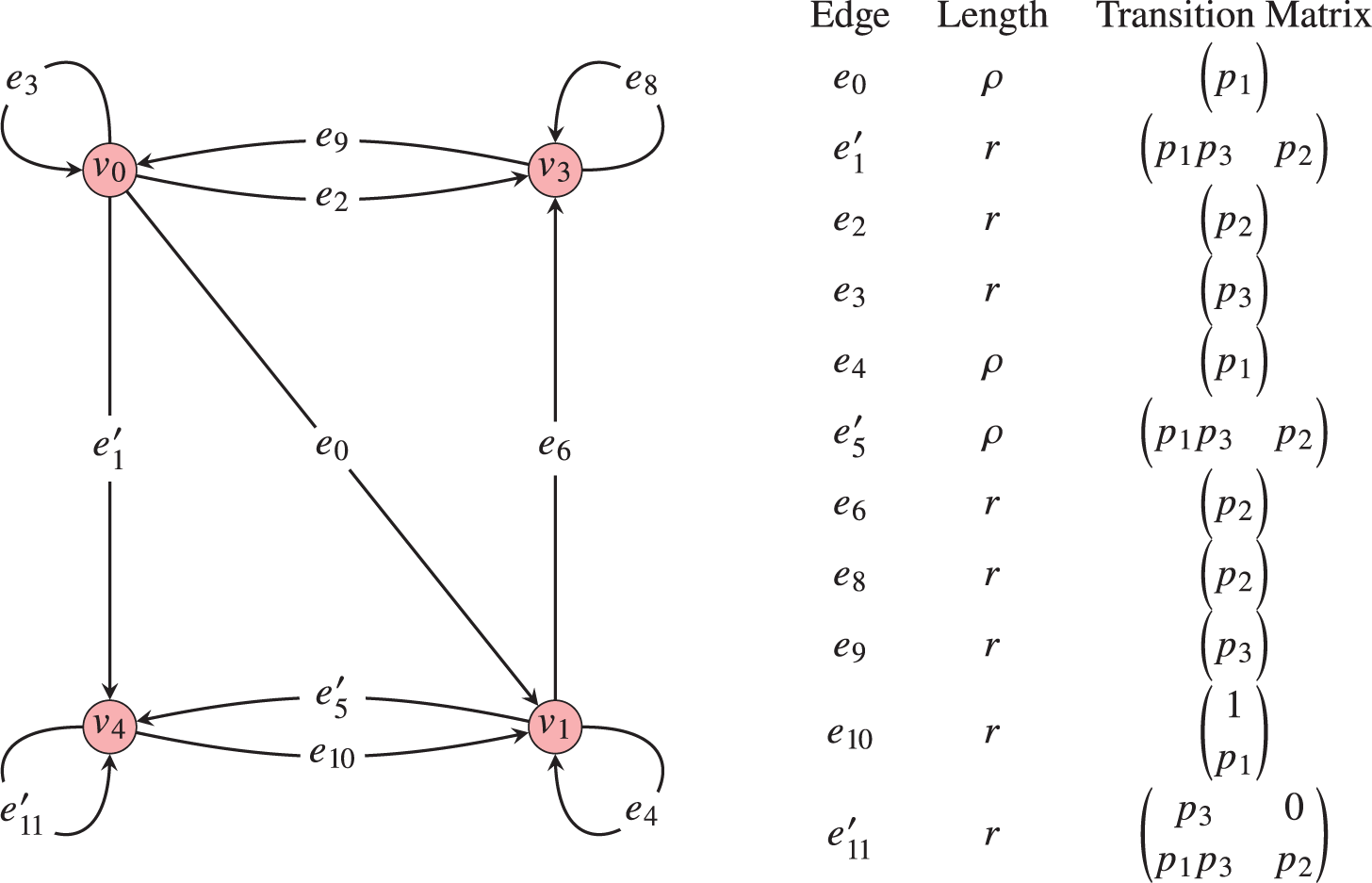
Figure 1 Modified transition graph with edge lengths and transition matrices.
5.3.2 The attainable local dimensions
We see that the conditions for Corollary 4.13 are satisfied, so that the measure ${\mu _{\boldsymbol {p}}}$
satisfies the complete multifractal formalism, and that the local dimensions at periodic points are dense in the set of upper and lower local dimensions.
${\mu _{\boldsymbol {p}}}$
satisfies the complete multifractal formalism, and that the local dimensions at periodic points are dense in the set of upper and lower local dimensions.
We now compute the range of local dimensions at periodic points. We first make note of the following obvious inequality: if $0<a,b,c,d$
and
$0<a,b,c,d$
and $\log a/\log b\leq \log c/\log d$
, then
$\log a/\log b\leq \log c/\log d$
, then
 $$ \begin{align} \frac{\log a}{\log b}\leq\frac{\log ac}{\log bd}\leq\frac{\log c}{\log d}. \end{align} $$
Now let $\eta $
be any cycle contained in
$\eta $
be any cycle contained in $\mathcal {G}$
. If
$\mathcal {G}$
. If $\eta $
only passes through
$\eta $
only passes through $v_{4}$
, since
$v_{4}$
, since $\operatorname {\mathrm {sp}}{T^{*}(e_{11}^{\prime })}=\max \{p_{2},p_{3}\}$
, the local dimension corresponding to the cycle
$\operatorname {\mathrm {sp}}{T^{*}(e_{11}^{\prime })}=\max \{p_{2},p_{3}\}$
, the local dimension corresponding to the cycle $(e_{11}^{\prime })$
is
$(e_{11}^{\prime })$
is ${\log \max \{p_{2},p_{3}\}}/{\log r}$
. Otherwise,
${\log \max \{p_{2},p_{3}\}}/{\log r}$
. Otherwise, $\eta $
passes through some vertex other than
$\eta $
passes through some vertex other than $v_{4}$
. Thus, without loss of generality,
$v_{4}$
. Thus, without loss of generality, $\eta $
begins and ends and some vertex
$\eta $
begins and ends and some vertex $v\neq v_{4}$
. Suppose
$v\neq v_{4}$
. Suppose $\eta $
visits some vertex
$\eta $
visits some vertex $w\neq v_{4}$
twice, that is,
$w\neq v_{4}$
twice, that is, $\eta =\eta _{1}\eta _{2}\eta _{3}$
, where
$\eta =\eta _{1}\eta _{2}\eta _{3}$
, where $\eta _{1}$
is a path from v to w,
$\eta _{1}$
is a path from v to w, $\eta _{2}$
is a cycle from w to w and
$\eta _{2}$
is a cycle from w to w and $\eta _{3}$
is a path from w to v. Then
$\eta _{3}$
is a path from w to v. Then $\eta $
can be written as a concatenation of cycles
$\eta $
can be written as a concatenation of cycles $\eta _{2}$
and
$\eta _{2}$
and $\eta _{3}\eta _{1}$
, where
$\eta _{3}\eta _{1}$
, where $T(\eta _{2})$
and
$T(\eta _{2})$
and $T(\eta _{3}\eta _{1})$
are singletons, and by equation (5.1), we have that
$T(\eta _{3}\eta _{1})$
are singletons, and by equation (5.1), we have that
 $$ \begin{align*} \min\bigg\{\frac{\log\operatorname{\mathrm{sp}} T(\eta_{2})}{\log L(\eta_{2})},\frac{\log\operatorname{\mathrm{sp}} T(\eta_{3}\eta_{1})}{\log L(\eta_{3}\eta_{1})}\bigg\}&\leq \frac{\log\operatorname{\mathrm{sp}} T(\eta)}{\log L(\eta)}\\[3pt] &\leq\max\bigg\{\frac{\log\operatorname{\mathrm{sp}} T(\eta_{2})}{\log L(\eta_{2})},\frac{\log\operatorname{\mathrm{sp}} T(\eta_{3}\eta_{1})}{\log L(\eta_{3}\eta_{1})}\bigg\}. \end{align*} $$
In other words, the minimum and maximum local dimensions on cycles are attained at cycles which do not repeat any vertex other than $v_{4}$
. Thus it suffices to consider all such families of cycles.
$v_{4}$
. Thus it suffices to consider all such families of cycles.
If $\eta $
does not pass through
$\eta $
does not pass through $v_{4}$
, the only non-repeating cycles are
$v_{4}$
, the only non-repeating cycles are $(e_{3})$
,
$(e_{3})$
, $(e_{4})$
,
$(e_{4})$
, $(e_{8})$
and
$(e_{8})$
and $(e_{2},e_{9})$
. We thus see that the maximum and minimum possible local dimensions are attained at the points in
$(e_{2},e_{9})$
. We thus see that the maximum and minimum possible local dimensions are attained at the points in
 $$ \begin{align*} S = \bigg\{\frac{\log p_{1}}{\log \rho},\frac{\log p_{2}}{\log r},\frac{\log p_{3}}{\log r}\bigg\}. \end{align*} $$
Otherwise, $\eta $
passes through
$\eta $
passes through $v_{4}$
. A straightforward induction argument shows that
$v_{4}$
. A straightforward induction argument shows that
 $$ \begin{align*} T^{*}(e_{11}^{\prime})^{n} = \begin{cases} \begin{pmatrix}p_{3}^{n} & 0\\[6pt] \dfrac{p_{1}p_{3}(p_{2}^{n}-p_{3}^{n})}{p_{2}-p_{3}}&p_{2}^{n}\end{pmatrix}, & p_{2}\neq p_{3},\\[22pt] \begin{pmatrix}p^{n}&0\\np^{n}p_{1} & p^{n}\end{pmatrix}, & p_{2}=p_{3}=:p. \end{cases} \end{align*} $$
Now, let
 $$ \begin{align*} \eta_{1,n}&=(e_{6},e_{9},e_{1}^{\prime},\underbrace{e_{11}^{\prime},\ldots,e_{11}^{\prime}}_{n},e_{10}) \quad \eta_{2,n}=(e_{5}^{\prime},\underbrace{e_{11}^{\prime},\ldots,e_{11}^{\prime}}_{n},e_{10}) \end{align*} $$
denote the two possible families of cycles which go through $v_{4}$
and do not repeat a vertex not in
$v_{4}$
and do not repeat a vertex not in $v_{4}$
. We then have that
$v_{4}$
. We then have that
 $$ \begin{align*} a_{n}:= \operatorname{\mathrm{sp}} T^{*}(\eta_{1,n})&= \begin{cases} \dfrac{p_{1}p_{2}p_{3}(p_{2}^{n+2}-p_{3}^{n+2})}{p_{2}-p_{3}}, & p_{2}\neq p_{3},\\[6pt] (2+n)p^{n+2}(1-2p)^{2}, & p_{2}=p_{3}=:p; \end{cases} \\[6pt] b_{n}:= \operatorname{\mathrm{sp}} T^{*}(\eta_{2,n})&= \begin{cases} \dfrac{p_{1}(p_{2}^{n+2}-p_{3}^{n+2})}{p_{2}-p_{3}}, & p_{2}\neq p_{3},\\[6pt] (2+n)p^{n+1}(1-2p)^{2}, & p_{2}=p_{3}=:p; \end{cases} \\[3pt] L(\eta_{1,n})&=r^{n+4};\\ L(\eta_{2,n})&= \rho r^{n+1}. \end{align*} $$
Let
 $$ \begin{align*}\begin{array}{ll} a_{\min} = \inf_{n}\dfrac{\log a_{n}}{(n+4)\log r}, & a_{\max} = \sup_{n}\dfrac{\log a_{n}}{(n+4)\log r},\\[12pt] b_{\min} = \inf_{n}\dfrac{\log b_{n}}{(n+1)\log r+\log\rho}, & b_{\max} = \sup_{n}\dfrac{\log b_{n}}{(n+1)\log r+\log\rho}. \end{array}\end{align*} $$
Then the minimal local dimension is equal to
 $$ \begin{align*} \alpha_{\min}:= \min\bigg\{\frac{\log p_{1}}{\log \rho},\frac{\log p_{2}}{\log r},\frac{\log p_{3}}{\log r},a_{\min},b_{\min}\bigg\} \end{align*} $$
and the maximal local dimension is equal to
 $$ \begin{align*} \alpha_{\max}:= \max\bigg\{\frac{\log p_{1}}{\log \rho},\frac{\log p_{2}}{\log r},\frac{\log p_{3}}{\log r},a_{\max},b_{\max}\bigg\}. \end{align*} $$
The parameters $\alpha _{\min }$
and
$\alpha _{\min }$
and $\alpha _{\max }$
can be determined exactly in many situations, but generic solutions are tedious. Additional details are left to the reader.
$\alpha _{\max }$
can be determined exactly in many situations, but generic solutions are tedious. Additional details are left to the reader.
5.3.3 The maximal open sets of the weak separation condition
Here we show, under the same assumption $\rho>r>\rho ^{2}$
that the essential net interval
$\rho>r>\rho ^{2}$
that the essential net interval $[0,1]\cap K$
is not contained in a union of open balls
$[0,1]\cap K$
is not contained in a union of open balls $U_{0}$
satisfying the maximal value in equation (3.1). In fact, we show that for any
$U_{0}$
satisfying the maximal value in equation (3.1). In fact, we show that for any $\epsilon>0$
, the open set
$\epsilon>0$
, the open set $(1-\epsilon ,1)\cap K$
is not contained a finite union of such open balls. In addition, this shows that for any
$(1-\epsilon ,1)\cap K$
is not contained a finite union of such open balls. In addition, this shows that for any $U(x,t)$
with
$U(x,t)$
with $\#\mathcal {S}_{t}(U(x,t))$
maximal, we must have
$\#\mathcal {S}_{t}(U(x,t))$
maximal, we must have $1\notin U(x,t)$
, whereas
$1\notin U(x,t)$
, whereas $1\in K=K_{\operatorname {\mathrm {ess}}}$
. A similar argument gives this result for general parameters
$1\in K=K_{\operatorname {\mathrm {ess}}}$
. A similar argument gives this result for general parameters $\rho $
and r, but the details are tedious and we omit the proof.
$\rho $
and r, but the details are tedious and we omit the proof.
We first note that $\sup _{x\in {\mathbb {R}},t>0}\#\mathcal {S}_{t}(U(x,t))\geq 5$
. To see this, take
$\sup _{x\in {\mathbb {R}},t>0}\#\mathcal {S}_{t}(U(x,t))\geq 5$
. To see this, take $t=1/4$
and
$t=1/4$
and $U_{0}:= U(1/4,1/4)$
. Then for each
$U_{0}:= U(1/4,1/4)$
. Then for each $\sigma \in \{11,12,13,22,23\}$
, we have
$\sigma \in \{11,12,13,22,23\}$
, we have $S_{\sigma }(K)\cap U_{0}\neq \emptyset $
(since
$S_{\sigma }(K)\cap U_{0}\neq \emptyset $
(since $S_{13}=S_{21}$
, we exclude the word
$S_{13}=S_{21}$
, we exclude the word $21$
).
$21$
).
To show that $(1-\epsilon ,1)\cap K$
is not contained in a finite union of maximal open balls for each
$(1-\epsilon ,1)\cap K$
is not contained in a finite union of maximal open balls for each $\epsilon>0$
, since
$\epsilon>0$
, since $1$
is an accumulation point for K it suffices to show that if
$1$
is an accumulation point for K it suffices to show that if $t>0$
and
$t>0$
and $U(x,t)$
is any open ball such that
$U(x,t)$
is any open ball such that $x+t=1$
,
$x+t=1$
, $\#\mathcal {S}_{t}(U(x,t))<5$
. A direct check shows that for
$\#\mathcal {S}_{t}(U(x,t))<5$
. A direct check shows that for $t>1/4$
,
$t>1/4$
, $\#\mathcal {S}_{t}(U(x,t))<5$
. Otherwise, let
$\#\mathcal {S}_{t}(U(x,t))<5$
. Otherwise, let $m\geq 1$
be such that
$m\geq 1$
be such that $1/4^{m+1}<t\leq 1/4^{m}$
. Since the rightmost child of
$1/4^{m+1}<t\leq 1/4^{m}$
. Since the rightmost child of $[0,1]$
is the net interval
$[0,1]$
is the net interval $[3/4,1]\in \Lambda _{1/4}$
with
$[3/4,1]\in \Lambda _{1/4}$
with ${\mathcal {V}}([3/4,1])={\mathcal {V}}([0,1])$
, the net interval in generation t containing
${\mathcal {V}}([3/4,1])={\mathcal {V}}([0,1])$
, the net interval in generation t containing $1$
is the interval
$1$
is the interval $\Delta =[1-1/4^{m},1]$
which has
$\Delta =[1-1/4^{m},1]$
which has ${\mathcal {V}}(\Delta )={\mathcal {V}}([0,1])$
, and thus
${\mathcal {V}}(\Delta )={\mathcal {V}}([0,1])$
, and thus $U(x,t)\subseteq \Delta ^{\prime }=[1-1/4^{m-1}]$
, where
$U(x,t)\subseteq \Delta ^{\prime }=[1-1/4^{m-1}]$
, where ${\mathcal {V}}(\Delta ^{\prime })={\mathcal {V}}([0,1])$
. However, then up to normalization, we know that the net intervals contained in
${\mathcal {V}}(\Delta ^{\prime })={\mathcal {V}}([0,1])$
. However, then up to normalization, we know that the net intervals contained in $\Delta ^{\prime }$
are the same as the net intervals contained in
$\Delta ^{\prime }$
are the same as the net intervals contained in $[0,1]$
so the case for general t reduces to the case
$[0,1]$
so the case for general t reduces to the case $t>1/4$
.
$t>1/4$
.
5.3.4 On the multifractal formalism
We now dispense with the assumptions on the parameters $\rho ,r$
and establish the following result.
$\rho ,r$
and establish the following result.
Theorem 5.7. Any invariant measure ${\mu _{\boldsymbol {p}}}$
associated with the IFS
${\mu _{\boldsymbol {p}}}$
associated with the IFS
 $$ \begin{align*} S_{1}(x) &=\rho\cdot x, \quad S_{2}(x) = r\cdot x+\rho(1-r), \quad S_{3}(x) =r\cdot x+1-r, \end{align*} $$
where $0<\rho ,r<1$
satisfy
$0<\rho ,r<1$
satisfy $\rho +2r-\rho r \leq 1$
, satisfies the complete multifractal formalism.
$\rho +2r-\rho r \leq 1$
, satisfies the complete multifractal formalism.
Proof. By Corollary 4.13 and the following remark, since the IFS satisfies the weak separation condition, it suffices to show that the vertex $v_{0}:= \{x\mapsto x\}$
is contained in the essential class. As argued in §5.3.1, the net interval
$v_{0}:= \{x\mapsto x\}$
is contained in the essential class. As argued in §5.3.1, the net interval $[0,1]$
has children
$[0,1]$
has children
 $$ \begin{align*} (\Delta_{1}=[0,\rho(1-r)],\Delta_{2}=[\rho(1-r),\rho],\Delta_{3}=[\rho,\rho+r-\rho r],\Delta_{4}=[1-r,r]) \end{align*} $$
in $\mathcal {F}_{1}$
with neighbour sets
$\mathcal {F}_{1}$
with neighbour sets
 $$ \begin{align*}\begin{array}{ll} {\mathcal{V}}(\Delta_{1}) = \{x\mapsto x/(1-r)\}, & {\mathcal{V}}(\Delta_{2}) = \bigg\{x\mapsto x/\rho,x\mapsto x/r+\dfrac{1}{r}-1\bigg\},\\[12pt] {\mathcal{V}}(\Delta_{3}) = \bigg\{x\mapsto\dfrac{x}{1-\rho}+\dfrac{\rho}{1-\rho}\bigg\}, & {\mathcal{V}}(\Delta_{4}) = \{x\mapsto x\}. \end{array}\end{align*} $$
In particular, there is an edge from $v_{0}$
to
$v_{0}$
to $v_{0}$
. Moreover, since the word
$v_{0}$
. Moreover, since the word $23$
is in
$23$
is in $\Lambda _{r}$
, where
$\Lambda _{r}$
, where $S_{23}([0,1])$
is disjoint from
$S_{23}([0,1])$
is disjoint from $S_{3}([0,1])$
,
$S_{3}([0,1])$
, $S_{22}([0,1])$
and
$S_{22}([0,1])$
and $S_{1}([0,1])$
by the assumptions on
$S_{1}([0,1])$
by the assumptions on $\rho $
and r, it follows that
$\rho $
and r, it follows that $S_{23}([0,1])$
is a net interval with neighbour set
$S_{23}([0,1])$
is a net interval with neighbour set $v_{0}$
. Thus there is an edge from
$v_{0}$
. Thus there is an edge from ${\mathcal {V}}(\Delta _{3})$
to
${\mathcal {V}}(\Delta _{3})$
to $v_{0}$
. Similarly, the words
$v_{0}$
. Similarly, the words $11$
and
$11$
and $12$
are in
$12$
are in $\Lambda _{\rho }$
, where
$\Lambda _{\rho }$
, where $S_{12}([0,1])$
is disjoint from
$S_{12}([0,1])$
is disjoint from $S_{2}([0,1])$
, so as computed in §5.3.1, the children of
$S_{2}([0,1])$
, so as computed in §5.3.1, the children of $\Delta _{1}$
have neighbour sets
$\Delta _{1}$
have neighbour sets ${\mathcal {V}}(\Delta _{1})$
,
${\mathcal {V}}(\Delta _{1})$
, ${\mathcal {V}}(\Delta _{2})$
and
${\mathcal {V}}(\Delta _{2})$
and ${\mathcal {V}}(\Delta _{3})$
. Since there is an edge from
${\mathcal {V}}(\Delta _{3})$
. Since there is an edge from ${\mathcal {V}}(\Delta _{3})$
to
${\mathcal {V}}(\Delta _{3})$
to $v_{0}$
, there is a path from
$v_{0}$
, there is a path from ${\mathcal {V}}(\Delta _{1})$
to
${\mathcal {V}}(\Delta _{1})$
to $v_{0}$
.
$v_{0}$
.
It remains to consider the offspring of $v_{2}:= {\mathcal {V}}(\Delta _{2})$
. We will treat the case where
$v_{2}:= {\mathcal {V}}(\Delta _{2})$
. We will treat the case where $r>\rho $
; the case where
$r>\rho $
; the case where $r\leq \rho $
follows by an analogous argument. Let m be maximal such that
$r\leq \rho $
follows by an analogous argument. Let m be maximal such that $r^{m}>\rho $
. We will compute the net intervals in generation
$r^{m}>\rho $
. We will compute the net intervals in generation $\Lambda _{r^{m}}$
.
$\Lambda _{r^{m}}$
.
For $0\leq k\leq m$
, write
$0\leq k\leq m$
, write
 $$ \begin{align*} \sigma_{k} &= \underbrace{2\ldots 2}_{k\text{ times}}1, \quad\tau_{k} = \underbrace{2\ldots 2}_{k\text{ times}}. \end{align*} $$
For simplicity, given $t>0$
, write
$t>0$
, write $\Gamma _{t}=\{S_{\omega }:\omega \in \Lambda _{t},S_{\omega }((0,1))\cap \Delta _{2}\neq \emptyset \}$
. Note that
$\Gamma _{t}=\{S_{\omega }:\omega \in \Lambda _{t},S_{\omega }((0,1))\cap \Delta _{2}\neq \emptyset \}$
. Note that $S_{2}(S_{1}(1))=S_{1}(1)$
, where
$S_{2}(S_{1}(1))=S_{1}(1)$
, where $S_{1}(1)$
is the right endpoint of
$S_{1}(1)$
is the right endpoint of $\Delta _{2}$
, so that
$\Delta _{2}$
, so that $S_{\sigma _{k}}(S_{1}(1))=S_{1}(1)$
. Thus by choice of m, we have for
$S_{\sigma _{k}}(S_{1}(1))=S_{1}(1)$
. Thus by choice of m, we have for $k\leq m$
,
$k\leq m$
,
 $$ \begin{align*} \Gamma_{r^{k}}=\{S_{\tau_{k+1}},S_{\sigma_{0}},S_{\sigma_{1}},\ldots,S_{\sigma_{k}}\}. \end{align*} $$
First assume $r^{m+1}<\rho $
. Since
$r^{m+1}<\rho $
. Since $r^{m+1}<\rho $
and
$r^{m+1}<\rho $
and $S_{1}([0,1])\supseteq \Delta _{2}\supseteq \Delta ^{i}$
,
$S_{1}([0,1])\supseteq \Delta _{2}\supseteq \Delta ^{i}$
, $\operatorname {\mathrm {tg}}(\Delta ^{i})=\rho $
. Thus since
$\operatorname {\mathrm {tg}}(\Delta ^{i})=\rho $
. Thus since $S_{12}(1)\leq S_{2}(0)$
and
$S_{12}(1)\leq S_{2}(0)$
and $S_{\sigma _{0} 2}=S_{\sigma _{1}}$
, we have
$S_{\sigma _{0} 2}=S_{\sigma _{1}}$
, we have
 $$ \begin{align*} \Gamma_{\rho}=\{\tau_{m+1},S_{\sigma_{1}},\ldots,S_{\sigma_{m}}\}. \end{align*} $$
Since $S_{\tau }(0)>S_{\sigma _{m}}(1)$
, the net intervals in
$S_{\tau }(0)>S_{\sigma _{m}}(1)$
, the net intervals in $\mathcal {F}_{\rho }$
contained in
$\mathcal {F}_{\rho }$
contained in $\Delta _{2}$
are given, ordered from left to right,
$\Delta _{2}$
are given, ordered from left to right,
 $$ \begin{align*} \Delta^{i} &=[S_{\sigma_{i}}(0),S_{\sigma_{i+1}}(0)], \quad \Delta^{m} = [S_{\sigma_{m}}(0),S_{\tau}(0)], \quad \Delta^{m+1} = [S_{\tau}(0),S_{\sigma_{m}}(1)] \end{align*} $$
for $1\leq i<m$
. Since
$1\leq i<m$
. Since $\Gamma _{r^{m-1}}=\{S_{2}^{-1}\circ g:g\in \Gamma _{\rho }\}$
, for each
$\Gamma _{r^{m-1}}=\{S_{2}^{-1}\circ g:g\in \Gamma _{\rho }\}$
, for each $1\leq i\leq m+1$
,
$1\leq i\leq m+1$
, $S_{2}^{-1}(\Delta ^{i})\in \mathcal {F}_{r^{m-1}}$
with
$S_{2}^{-1}(\Delta ^{i})\in \mathcal {F}_{r^{m-1}}$
with ${\mathcal {V}}(S_{2}^{-1}(\Delta ^{i}))={\mathcal {V}}(\Delta ^{i})$
. However, again
${\mathcal {V}}(S_{2}^{-1}(\Delta ^{i}))={\mathcal {V}}(\Delta ^{i})$
. However, again $S_{2}$
fixes the right endpoint of
$S_{2}$
fixes the right endpoint of $\Delta _{2}$
, so that
$\Delta _{2}$
, so that
 $$ \begin{align*} \Delta_{2}\supseteq S_{2}^{-1}(\Delta^{i})\supseteq\Delta^{j} \end{align*} $$
for each $2\leq i\leq m+1$
. In particular, every child of
$2\leq i\leq m+1$
. In particular, every child of ${\mathcal {V}}(\Delta ^{i})$
is of the form
${\mathcal {V}}(\Delta ^{i})$
is of the form ${\mathcal {V}}(\Delta ^{j})$
, and there is a path from
${\mathcal {V}}(\Delta ^{j})$
, and there is a path from ${\mathcal {V}}(\Delta ^{i})$
to
${\mathcal {V}}(\Delta ^{i})$
to ${\mathcal {V}}(\Delta ^{1})$
for each
${\mathcal {V}}(\Delta ^{1})$
for each $i\geq 2$
. Moreover, a direct computation shows that
$i\geq 2$
. Moreover, a direct computation shows that ${\mathcal {V}}(\Delta ^{1})={\mathcal {V}}(\Delta _{1})$
, so there is a path from
${\mathcal {V}}(\Delta ^{1})={\mathcal {V}}(\Delta _{1})$
, so there is a path from ${\mathcal {V}}(\Delta ^{1})$
to
${\mathcal {V}}(\Delta ^{1})$
to $v_{0}$
. Thus there are no new net intervals, and there is a path to
$v_{0}$
. Thus there are no new net intervals, and there is a path to $v_{0}=\{x\mapsto x\}$
from any vertex in the transition graph, as required.
$v_{0}=\{x\mapsto x\}$
from any vertex in the transition graph, as required.
In the case $r^{m+1}=\rho $
, we get
$r^{m+1}=\rho $
, we get
 $$ \begin{align*} \Gamma_{\rho}=\{\tau_{m+2},S_{\sigma_{1}},\ldots,S_{\sigma_{m+1}}\}, \end{align*} $$
so that $\Gamma _{\rho }$
is a rescaled version of
$\Gamma _{\rho }$
is a rescaled version of $\Gamma _{r^{m}}$
, and the argument follows similarly.
$\Gamma _{r^{m}}$
, and the argument follows similarly.
5.4 On an example of Deng and Ngai
In [Reference Deng and Ngai4, Example 8.5], Deng and Ngai introduced the following IFS similar in structure to §5.3 but with an additional overlap. Consider IFS defined by following four maps
 $$ \begin{align*}\begin{array}{ll} S_{1}(x) = \rho x, & S_{2}(x) = rx+\rho(1-r),\\[4pt] S_{3}(x) = \rho^{-1}r^{2} x+(1-r)(\rho+r), & S_{4}(x) = rx+(1-r), \end{array}\end{align*} $$
where $0<\rho ,r\in <1$
satisfy
$0<\rho ,r\in <1$
satisfy $r^{2}<\rho $
and
$r^{2}<\rho $
and $\rho (r-1)(\rho +r-1)>r^{2}$
. The constraints on
$\rho (r-1)(\rho +r-1)>r^{2}$
. The constraints on $\rho $
and r ensure that
$\rho $
and r ensure that $S_{3}((0,1))\cap S_{4}((0,1))=\emptyset $
.
$S_{3}((0,1))\cap S_{4}((0,1))=\emptyset $
.
The parameters of this IFS are chosen so that $S_{14}=S_{21}$
and
$S_{14}=S_{21}$
and $S_{24}=S_{31}$
. One can verify, arguing similarly to Theorem 5.7, that
$S_{24}=S_{31}$
. One can verify, arguing similarly to Theorem 5.7, that $\mathcal {G}=\mathcal {G}_{\operatorname {\mathrm {ess}}}$
and hence any associated self-similar measure satisfies the complete multifractal formalism.
$\mathcal {G}=\mathcal {G}_{\operatorname {\mathrm {ess}}}$
and hence any associated self-similar measure satisfies the complete multifractal formalism.
5.5 A modified multifractal formalism for Cantor-like measures
Consider the family of IFS given by maps
 $$ \begin{align*} \bigg\{S_{j}(x)=\frac{x}{r}+\frac{j}{mr}(r-1):0\leq j\leq m\bigg\}, \end{align*} $$
where $m\geq r\geq 2$
and
$m\geq r\geq 2$
and $m,r$
are integers. This family of IFS, with appropriate probabilities, contains rescaled versions of measures such as convolutions of the usual Cantor measure. In particular, certain self-similar measures in this family were among the first recognized for which the multifractal formalism can fail [Reference Hu and Lau24]. The set of local dimensions is known to consist of a closed interval and, with appropriate probabilities, an isolated point. The
$m,r$
are integers. This family of IFS, with appropriate probabilities, contains rescaled versions of measures such as convolutions of the usual Cantor measure. In particular, certain self-similar measures in this family were among the first recognized for which the multifractal formalism can fail [Reference Hu and Lau24]. The set of local dimensions is known to consist of a closed interval and, with appropriate probabilities, an isolated point. The $L^{q}$
-spectra have also been computed, as well as a modified multifractal formalism [Reference Feng and Lau13, Reference Feng, Lau and Wang14, Reference Lau and Wang31, Reference Shmerkin38]; our results here are minor improvements of existing results and are primarily useful as illustrations of the theorems.
$L^{q}$
-spectra have also been computed, as well as a modified multifractal formalism [Reference Feng and Lau13, Reference Feng, Lau and Wang14, Reference Lau and Wang31, Reference Shmerkin38]; our results here are minor improvements of existing results and are primarily useful as illustrations of the theorems.
Fix any IFS $\{S_{i}\}_{i\in \mathcal {I}}$
in this family with attractor K and associated self-similar measure
$\{S_{i}\}_{i\in \mathcal {I}}$
in this family with attractor K and associated self-similar measure $\mu $
. Arguing similarly to [Reference Hare, Hare and Matthews18, Proposition 7.1], one may verify that
$\mu $
. Arguing similarly to [Reference Hare, Hare and Matthews18, Proposition 7.1], one may verify that $K=[0,1]$
,
$K=[0,1]$
, $K_{\operatorname {\mathrm {ess}}}=(0,1)$
and
$K_{\operatorname {\mathrm {ess}}}=(0,1)$
and
 $$ \begin{align*} K_{m}:= \bigcup_{\substack{\Delta\in\mathcal{F}_{r^{m-1}}\\ {\mathcal{V}}(\Delta)\in V(\mathcal{G}_{\operatorname{\mathrm{ess}}})}}=\bigg[\frac{r-1}{kr^{m}},1-\frac{(r-1)}{kr^{m}}\bigg]. \end{align*} $$
Then Theorem 4.11 (weak regularity is always satisfied since $K=[0,1])$
gives that each
$K=[0,1])$
gives that each $\mu _{m}:= {\mu _{\boldsymbol {p}}}|_{K_{m}}$
satisfies the complete multifractal formalism and
$\mu _{m}:= {\mu _{\boldsymbol {p}}}|_{K_{m}}$
satisfies the complete multifractal formalism and
 $$ \begin{align*} D(\mu_{m})=\{{\dim_{\operatorname{\mathrm{loc}}}}{\mu_{\boldsymbol{p}}}(x):x\in(0,1)\}. \end{align*} $$
This provides an alternative proof of some of the results contained in [Reference Feng, Lau and Wang14, Reference Shmerkin38] (without the assumption $k<2r-2$
) and a variation of [Reference Feng and Lau13, Example 6.2].
$k<2r-2$
) and a variation of [Reference Feng and Lau13, Example 6.2].
From the perspective of Corollary 4.13, the obstruction to the multifractal formalism is combinatorial: there is a cycle outside the essential class which contributes a point with local dimension not contained in the closed interval $\{{\dim _{\operatorname {\mathrm {loc}}}}\mu (x):x\in K_{\operatorname {\mathrm {ess}}}\}$
.
$\{{\dim _{\operatorname {\mathrm {loc}}}}\mu (x):x\in K_{\operatorname {\mathrm {ess}}}\}$
.
Acknowledgements
A.R. would like to thank Kathryn Hare and Kevin Hare for their support and frequent discussions concerning many of the topics in this paper. The author also thanks an anonymous referee for pointing out an error in a prior version of Theorem 1.2, and for comments which suggested the current version. This project was supported by NSERC Grants RGPIN-2016-03719 (K.E. Hare) and RGPIN-2019- 03930 (K.G. Hare).


 Open access