


1. Introduction
The search for a global minimiser $v^*$
of a potentially non-convex and non-smooth cost function
$v^*$
of a potentially non-convex and non-smooth cost function
 \begin{equation*}{f}\,:\,\mathbb {R}^d\to \mathbb {R}\end{equation*}
holds significant importance in a variety of applications throughout applied mathematics, science and technology, engineering, and machine learning. Historically, a class of methods known as metaheuristics [Reference Bäck, Fogel and Michalewicz1, Reference Blum and Roli2] has been developed to address this inherently challenging and, in general, NP-hard problem. Examples of such include evolutionary programming [Reference Fogel3], genetic algorithms [Reference Holland4], particle swarm optimisation (PSO) [Reference Kennedy and Eberhart5], simulated annealing [Reference Aarts and Korst6] and many others. These methods work by combining local improvement procedures and global strategies by orchestrating deterministic and stochastic advances, with the aim of creating a method capable of robustly and efficiently finding the globally minimising argument $v^*$
of
$v^*$
of $f$
. However, despite their empirical success and widespread adoption in practice, most metaheuristics lack a solid mathematical foundation that could guarantee their robust convergence to global minimisers under reasonable assumptions.
$f$
. However, despite their empirical success and widespread adoption in practice, most metaheuristics lack a solid mathematical foundation that could guarantee their robust convergence to global minimisers under reasonable assumptions.
Motivated by the urge to devise algorithms which converge provably, a novel class of metaheuristics, so-called consensus-based optimisation (CBO), originally proposed by the authors of [Reference Pinnau, Totzeck, Tse and Martin7], has recently emerged in the literature. Due to the inherent simplicity in the design of CBO, this class of optimisation algorithms lends itself to a rigorous theoretical analysis, as demonstrated in particular in the works [Reference Carrillo, Choi, Totzeck and Tse8–Reference Ko, Ha, Jin and Kim14]. However, this recent line of research does not just offer a promising avenue for establishing a thorough mathematical framework for understanding the numerically observed successes of CBO methods [Reference Carrillo, Jin, Li and Zhu9, Reference Fornasier, Klock, Riedl, Laredo, Hidalgo and Babaagba11, Reference Carrillo, Trillos, Li and Zhu15–Reference Riedl17], but beyond that allows to explain the effective use of conceptually similar and widespread methods such as PSO as well as at first glance completely different optimisation algorithms such as stochastic gradient descent (SGD). While the first connection is to be expected and by now made fairly rigorous [Reference Cipriani, Huang and Qiu18–Reference Huang, Qiu and Riedl20] due to CBO indisputably taking PSO as inspiration, the second observation is somewhat surprising, as it builds a bridge between derivative-free metaheuristics and gradient-based learning algorithms. Despite CBO solely relying on evaluations of the objective function, recent work [Reference Riedl, Klock, Geldhauser and Fornasier21] reveals an intrinsic SGD-like behaviour of CBO itself by interpreting it as a certain stochastic relaxation of gradient descent, which provably overcomes energy barriers of non-convex function. These perspectives, and, in particular, the already well-investigated convergence behaviour of standard CBO, encourage the exploration of improvements to the method in order to allow overcoming the limitations of traditional metaheuristics mentioned at the start. For recent surveys on CBO, we refer to [Reference Grassi, Huang, Pareschi and Qiu22, Reference Totzeck23].
While the original CBO model [Reference Pinnau, Totzeck, Tse and Martin7] has been adapted to solve constrained optimisations [Reference Bae, Ha, Kang, Lim, Min and Yoo24–Reference Carrillo, Totzeck and Vaes26], optimisations on manifolds [Reference Fornasier, Huang, Pareschi and Sünnen16, Reference Fornasier, Huang, Pareschi and Sünnen27–Reference Kim, Kang, Kim, Ha and Yang30], multi-objective optimisation problems [Reference Borghi, Herty and Pareschi31–Reference Klamroth, Stiglmayr and Totzeck33], saddle point problems [Reference Huang, Qiu and Riedl34] or the task of sampling [Reference Carrillo, Hoffmann, Stuart and Vaes35], as well as has been extended to make use of memory mechanisms [Reference Riedl17, Reference Borghi, Grassi and Pareschi36, Reference Totzeck and Wolfram37], gradient information [Reference Riedl17, Reference Schillings, Totzeck and Wacker38], momentum [Reference Chen, Jin and Lyu39], jump-diffusion processes [Reference Kalise, Sharma and Tretyakov40] or localisation kernels for polarisation [Reference Bungert, Wacker and Roith41], we focus in this work on a variation of the original model, which incorporates a truncation in the noise term of the dynamics. More formally, given a time horizon $T\gt 0$
, a time discretisation
$T\gt 0$
, a time discretisation $t_0 = 0 \lt \Delta t \lt \cdots \lt K \Delta t = t_K = T$
of
$t_0 = 0 \lt \Delta t \lt \cdots \lt K \Delta t = t_K = T$
of $[0,T]$
, and user-specified parameters
$[0,T]$
, and user-specified parameters $\alpha,\lambda,\sigma \gt 0$
as well as
$\alpha,\lambda,\sigma \gt 0$
as well as $v_b,R\gt 0$
, we consider the interacting particle system
$v_b,R\gt 0$
, we consider the interacting particle system
 \begin{align} {V^i_{{k+1,\Delta t}} - V^i_{{k,\Delta t}}} = - \Delta t\lambda \!\left ( V^i_{{k,\Delta t}} - \mathcal{P}_{v_b,R}\!\left (v_{\alpha }\!\left({\widehat \rho ^{\,N}_{{k,\Delta t}}}\right)\right )\right ) + \sigma \!\left (\left \|{ V^i_{{k,\Delta t}}-v_{\alpha }\!\left({\widehat \rho ^{\,N}_{{k,\Delta t}}}\right)}\right \|_2 \wedge M\right ) B^i_{{k,\Delta t}}, \end{align}
 \begin{align}{V_0^i} &\sim \rho _0 \quad \text{for all } i =1,\ldots,N, \end{align}
where $(( B^i_{{k,\Delta t}})_{k=0,\ldots,K-1})_{i=1,\ldots,N}$
are independent, identically distributed Gaussian random vectors in
$(( B^i_{{k,\Delta t}})_{k=0,\ldots,K-1})_{i=1,\ldots,N}$
are independent, identically distributed Gaussian random vectors in $\mathbb{R}^d$
with zero mean and covariance matrix
$\mathbb{R}^d$
with zero mean and covariance matrix $\Delta t \mathsf{Id}_d$
. Equation (1) originates from a simple Euler–Maruyama time discretisation [Reference Higham42, Reference Platen43] of the system of stochastic differential equations (SDEs), expressed in Itô’s form as
$\Delta t \mathsf{Id}_d$
. Equation (1) originates from a simple Euler–Maruyama time discretisation [Reference Higham42, Reference Platen43] of the system of stochastic differential equations (SDEs), expressed in Itô’s form as
 \begin{align} d V^i_t = -\lambda \!\left (V^i_t-\mathcal{P}_{v_b,R}\!\left (v_{\alpha }\!\left(\widehat{\rho }_t^N\right)\right )\right )dt+\sigma \!\left (\left \| V^i_t-v_{\alpha }\!\left(\widehat \rho ^{\,N}_{t}\right) \right \|_2\wedge M\right )dB^i_t \end{align}
 \begin{align}{V_0^i} &\sim \rho _0 \quad \text{for all } i =1,\ldots,N, \end{align}
where $((B_t^i)_{t\geq 0})_{i = 1,\ldots,N}$
are now independent standard Brownian motions in
$((B_t^i)_{t\geq 0})_{i = 1,\ldots,N}$
are now independent standard Brownian motions in $\mathbb{R}^d$
. The empirical measure of the particles at time
$\mathbb{R}^d$
. The empirical measure of the particles at time $t$
is denoted by
$t$
is denoted by $\widehat \rho ^{\,N}_{t} \,:\!=\, \frac{1}{N} \sum _{i=1}^{N} \delta _{V_t^i}$
. Moreover,
$\widehat \rho ^{\,N}_{t} \,:\!=\, \frac{1}{N} \sum _{i=1}^{N} \delta _{V_t^i}$
. Moreover, $\mathcal{P}_{v_b,R}$
is the projection onto
$\mathcal{P}_{v_b,R}$
is the projection onto $B_R(v_b)$
defined as
$B_R(v_b)$
defined as
 \begin{equation} \mathcal{P}_{v_b,R}\!\left (v\right )\,:\!=\, \begin{cases} v, & \text{if $\left \|{v-v_b}\right \|_2\leq R$},\\[6pt] v_b+R\dfrac{v-v_b}{\left \|{v-v_b}\right \|_2}, & \text{if $\left \|{v-v_b}\right \|_2\gt R$}. \end{cases} \end{equation}
As a crucial assumption in this paper, the map $\mathcal{P}_{v_b,R}$
depends on
$\mathcal{P}_{v_b,R}$
depends on $R$
and
$R$
and $v_b$
in such way that
$v_b$
in such way that $v^*\in B_R(v_b)$
. Setting the parameters can be feasible under specific circumstances, as exemplified by the regularised optimisation problem
$v^*\in B_R(v_b)$
. Setting the parameters can be feasible under specific circumstances, as exemplified by the regularised optimisation problem $f(v)\,:\!=\,\operatorname{Loss}(v)+ \Lambda \!\left \| v \right \|_2$
, wherein
$f(v)\,:\!=\,\operatorname{Loss}(v)+ \Lambda \!\left \| v \right \|_2$
, wherein $v^*\in B_{\operatorname{Loss}(0)/ \Lambda }(0)$
. In the absence of prior knowledge regarding
$v^*\in B_{\operatorname{Loss}(0)/ \Lambda }(0)$
. In the absence of prior knowledge regarding $v_b$
and
$v_b$
and $R$
, a practical approach is to choose
$R$
, a practical approach is to choose $v_b=0$
and assign a sufficiently large value to
$v_b=0$
and assign a sufficiently large value to $R$
. The first terms in (1) and (3), respectively, impose a deterministic drift of each particle towards the possibly projected momentaneous consensus point
$R$
. The first terms in (1) and (3), respectively, impose a deterministic drift of each particle towards the possibly projected momentaneous consensus point $v_{\alpha }\big({\widehat \rho ^{\,N}_{t}}\big)$
, which is a weighted average of the particles’ positions and computed according to
$v_{\alpha }\big({\widehat \rho ^{\,N}_{t}}\big)$
, which is a weighted average of the particles’ positions and computed according to
 \begin{align} v_{\alpha }\big({\widehat \rho ^{\,N}_{t}}\big) \,:\!=\, \int v \frac{\omega _{\alpha }(v)}{\left \|{\omega _{\alpha }}\right \|_{L_1\!\left(\widehat \rho ^{\,N}_{t}\right)}}\,d\widehat \rho ^{\,N}_{t}(v). \end{align}
The weights $ \omega _{\alpha }(v)\,:\!=\,\exp \!({-}\alpha{f}(v))$
are motivated by the well-known Laplace principle [Reference Dembo and Zeitouni44], which states for any absolutely continuous probability distribution
$ \omega _{\alpha }(v)\,:\!=\,\exp \!({-}\alpha{f}(v))$
are motivated by the well-known Laplace principle [Reference Dembo and Zeitouni44], which states for any absolutely continuous probability distribution $\varrho$
on
$\varrho$
on $\mathbb{R}^d$
that
$\mathbb{R}^d$
that
 \begin{align} \lim \limits _{\alpha \rightarrow \infty }\left ({-}\frac{1}{\alpha }\log \!\left (\int \omega _{\alpha }(v)\,d\varrho (v)\right )\right ) = \inf \limits _{v \in \operatorname{supp}(\varrho )}{f}(v) \end{align}
and thus justifies that $v_{\alpha }\big({\widehat \rho ^{\,N}_{t}}\big)$
serves as a suitable proxy for the global minimiser
$v_{\alpha }\big({\widehat \rho ^{\,N}_{t}}\big)$
serves as a suitable proxy for the global minimiser $v^*$
given the currently available information of the particles
$v^*$
given the currently available information of the particles $(V^i_t)_{i=1,\dots,N}$
. The second terms in (1) and (3), respectively, encode the diffusion or exploration mechanism of the algorithm, where, in contrast to standard CBO, we truncate the noise by some fixed constant
$(V^i_t)_{i=1,\dots,N}$
. The second terms in (1) and (3), respectively, encode the diffusion or exploration mechanism of the algorithm, where, in contrast to standard CBO, we truncate the noise by some fixed constant $M\gt 0$
.
$M\gt 0$
.
We conclude and re-iterate that both the introduction of the projection $\mathcal{P}_{v_b,R}\!\left (v_{\alpha }\!\left(\widehat{\rho }_t^N\right)\right )$
of the consensus point and the employment of truncation of the noise variance
$\mathcal{P}_{v_b,R}\!\left (v_{\alpha }\!\left(\widehat{\rho }_t^N\right)\right )$
of the consensus point and the employment of truncation of the noise variance $\left (\,\!\left \| V^i_t-v_{\alpha }\left(\widehat \rho ^{\,N}_{t}\right) \right \|_2\wedge M\right )$
are main innovations to the original CBO method. We shall explain and justify these modifications in the following paragraph.
$\left (\,\!\left \| V^i_t-v_{\alpha }\left(\widehat \rho ^{\,N}_{t}\right) \right \|_2\wedge M\right )$
are main innovations to the original CBO method. We shall explain and justify these modifications in the following paragraph.
Despite these technical improvements, the approach to analyse the convergence behaviour of the implementable scheme (1) follows a similar route already explored in [Reference Carrillo, Choi, Totzeck and Tse8–Reference Fornasier, Klock, Riedl, Laredo, Hidalgo and Babaagba11]. In particular, the convergence behaviour of the method to the global minimiser $v^*$
of the objective
$v^*$
of the objective $f$
is investigated on the level of the mean-field limit [Reference Fornasier, Klock and Riedl10, Reference Huang and Qiu45] of the system (3). More precisely, we study the macroscopic behaviour of the agent density
$f$
is investigated on the level of the mean-field limit [Reference Fornasier, Klock and Riedl10, Reference Huang and Qiu45] of the system (3). More precisely, we study the macroscopic behaviour of the agent density $\rho \in{\mathcal{C}}([0,T],{\mathcal{P}}(\mathbb{R}^d))$
, where
$\rho \in{\mathcal{C}}([0,T],{\mathcal{P}}(\mathbb{R}^d))$
, where $\rho _t=\textrm{Law}(\overline{V}_t)$
with
$\rho _t=\textrm{Law}(\overline{V}_t)$
with
 \begin{equation} d\overline{V}_t=-\lambda \!\left (\overline{V}_t-\mathcal{P}_{v_b,R}\!\left (v_{\alpha }(\rho _t)\right )\right )dt+\sigma \!\left (\left \|{\overline{V}_t-v_{\alpha }(\rho _t)}\right \|_2\wedge M\right )d B_t \end{equation}
and initial data $\overline{V}_0\sim \rho _0$
. Afterwards, by establishing a quantitative estimate on the mean-field approximation, that is, the proximity of the mean-field system (8) to the interacting particle system (3) and combining the two results, we obtain a convergence result for the CBO algorithm (1) with truncated noise.
$\overline{V}_0\sim \rho _0$
. Afterwards, by establishing a quantitative estimate on the mean-field approximation, that is, the proximity of the mean-field system (8) to the interacting particle system (3) and combining the two results, we obtain a convergence result for the CBO algorithm (1) with truncated noise.
1.1. Motivation for using truncated noise
In what follows, we provide a heuristic explanation of the theoretical benefits of employing a truncation in the noise of CBO as in (1), (3) and (8). Let us therefore first recall that the standard variant of CBO [Reference Pinnau, Totzeck, Tse and Martin7] can be retrieved from the model considered in this paper by setting $v_b=0$
,
$v_b=0$
, $ R=\infty$
and
$ R=\infty$
and $M=\infty$
. For instance, in place of the mean-field dynamics (8), we would have
$M=\infty$
. For instance, in place of the mean-field dynamics (8), we would have
 \begin{equation*} d \overline {V}^{\text {CBO}}_t =-\lambda \!\left (\overline {V}^{\text {CBO}}_t-v_{\alpha }\big({\rho ^{\text {CBO}}_t}\big)\right )dt+\sigma \!\left \|{\overline {V}^{\text {CBO}}_t-v_{\alpha }\big({\rho ^{\text {CBO}}_t}\big)}\right \|_2 d B_t. \end{equation*}
Attributed to the Laplace principle (7), it holds $v_{\alpha }({\rho ^{\text{CBO}}_t})\approx v^*$
for
$v_{\alpha }({\rho ^{\text{CBO}}_t})\approx v^*$
for $\alpha$
sufficiently large, that is, as
$\alpha$
sufficiently large, that is, as $\alpha \rightarrow \infty$
, the former dynamics converges to
$\alpha \rightarrow \infty$
, the former dynamics converges to
 \begin{equation} d \overline{Y}^{\text{CBO}}_t=-\lambda \!\left (\overline{Y}^{\text{CBO}}_t-v^*\right )dt+\sigma \!\left \|{\overline{Y}^{\text{CBO}}_t-v^*}\right \|_2d B_t. \end{equation}
First, observe that here the first term imposes a direct drift to the global minimiser $v^*$
and thereby induces a contracting behaviour, which is on the other hand counteracted by the diffusion term, which contributes a stochastic exploration around this point. In particular, with
$v^*$
and thereby induces a contracting behaviour, which is on the other hand counteracted by the diffusion term, which contributes a stochastic exploration around this point. In particular, with $\overline{Y}^{\text{CBO}}_t$
approaching
$\overline{Y}^{\text{CBO}}_t$
approaching $v^*$
, the exploration vanishes so that
$v^*$
, the exploration vanishes so that $\overline{Y}^{\text{CBO}}_t$
converges eventually deterministically to
$\overline{Y}^{\text{CBO}}_t$
converges eventually deterministically to $v^*$
. Conversely, as long as
$v^*$
. Conversely, as long as $\overline{Y}^{\text{CBO}}_t$
is far away from
$\overline{Y}^{\text{CBO}}_t$
is far away from $v^*$
, the order of the random exploration is strong. By Itô’s formula, we have
$v^*$
, the order of the random exploration is strong. By Itô’s formula, we have
 \begin{equation*} \frac {d}{dt}\mathbb {E}\!\left [\left \|{\overline {Y}^{\text {CBO}}_t-v^*}\right \|_2^p\right ] =p\!\left ({-}\lambda +\frac {\sigma ^2}{2}\left (p+d-2\right )\right )\mathbb {E}\!\left [\left \|{\overline {Y}^{\text {CBO}}_t-v^*}\right \|_2^p\right ] \end{equation*}
and thus
 \begin{equation} \mathbb{E}\!\left [\left \|{\overline{Y}^{\text{CBO}}_t-v^*}\right \|_2^p\right ] = \exp \!\left (p\!\left ({-}\lambda +\frac{\sigma ^2}{2}\left (p+d-2\right )\right )t\right ) \mathbb{E}\!\left [\left \|{\overline{Y}^{\text{CBO}}_0-v^*}\right \|_2^p\right ] \end{equation}
for any $p\geq 1$
. Denoting with
$p\geq 1$
. Denoting with $\mu ^{\text{CBO}}_t$
the law of
$\mu ^{\text{CBO}}_t$
the law of $\overline{Y}^{\text{CBO}}_t$
, this means that, given any
$\overline{Y}^{\text{CBO}}_t$
, this means that, given any $\lambda,\sigma \gt 0$
, there is some threshold exponent
$\lambda,\sigma \gt 0$
, there is some threshold exponent $p^*=p^*(\lambda,\sigma,d)$
, such that
$p^*=p^*(\lambda,\sigma,d)$
, such that
 \begin{align*} \begin{split} \lim _{t\to \infty } W_p\!\left (\mu ^{\text{CBO}}_t,\delta _{v^*}\right ) &=\lim _{t\to \infty }{\left (\mathbb{E}\!\left [\left \|{\overline{Y}^{\text{CBO}}_t-v^*}\right \|_2^p\right ]\right )}^{1/p} \\ &=\lim _{t\to \infty }\exp \!\left (\left ({-}\lambda +\frac{\sigma ^2}{2}\left (p+d-2\right )\right )t\right ){\left (\mathbb{E}\!\left [\left \|{\overline{Y}^{\text{CBO}}_0-v^*}\right \|_2^p\right ]\right )}^{1/p}\\ &=0 \end{split} \end{align*}
for $p\lt p^*$
, while for
$p\lt p^*$
, while for $p\gt p^*$
it holds
$p\gt p^*$
it holds
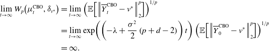 \begin{align*} \begin{split} \lim _{t\to \infty } W_p\!\left (\mu ^{\text{CBO}}_t,\delta _{v^*}\right ) &=\lim _{t\to \infty }{\left (\mathbb{E}\!\left [\left \|{\overline{Y}^{\text{CBO}}_t-v^*}\right \|_2^p\right ]\right )}^{1/p}\\ &=\lim _{t\to \infty }\exp \!\left (\left ({-}\lambda +\frac{\sigma ^2}{2}\left (p+d-2\right )\right )t\right ){\left (\mathbb{E}\!\left [\left \|{\overline{Y}^{\text{CBO}}_0-v^*}\right \|_2^p\right ]\right )}^{1/p}\\ &=\infty. \end{split} \end{align*}
Recalling that the distribution of a random variable $Y$
has heavy tails if and only if the moment generating function
$Y$
has heavy tails if and only if the moment generating function $M_Y(s)\,:\!=\,\mathbb{E}\!\left [\exp \!(sY)\right ] =\mathbb{E}\!\left [\sum _{p=0}^\infty (sY)^p/p!\right ]$
is infinite for all
$M_Y(s)\,:\!=\,\mathbb{E}\!\left [\exp \!(sY)\right ] =\mathbb{E}\!\left [\sum _{p=0}^\infty (sY)^p/p!\right ]$
is infinite for all $s\gt 0$
, these computations suggest that the distribution of
$s\gt 0$
, these computations suggest that the distribution of $\mu ^{\text{CBO}}_t$
exhibits characteristics of heavy tails as
$\mu ^{\text{CBO}}_t$
exhibits characteristics of heavy tails as $t\to \infty$
, thereby increasing the likelihood of encountering outliers in a sample drawn from
$t\to \infty$
, thereby increasing the likelihood of encountering outliers in a sample drawn from $\mu ^{\text{CBO}}_t$
for large
$\mu ^{\text{CBO}}_t$
for large $t$
.
$t$
.
On the contrary, for CBO with truncated noise (8), we get, thanks once again to the Laplace principle as $\alpha \rightarrow \infty$
, that (8) converges to
$\alpha \rightarrow \infty$
, that (8) converges to
 \begin{equation} d\overline{Y}_t =-\lambda \!\left (\overline{Y}_t-v^*\right )dt+\sigma \!\left (\left \|{\overline{Y}_t-v^*}\right \|_2\wedge M\right )dB_t, \end{equation}
for which we can compute
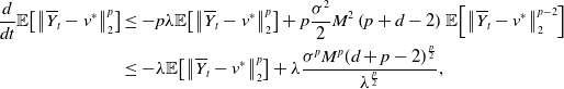 \begin{equation*} \begin{aligned} \frac{d}{dt}\mathbb{E}\!\left [\left \|{\overline{Y}_t-v^*}\right \|_2^p\right ] &\leq -p\lambda \mathbb{E}\!\left [\left \|{\overline{Y}_t-v^*}\right \|_2^p\right ]+p\frac{\sigma ^2}{2}M^2\left (p+d-2\right )\mathbb{E}\!\left [\left \|{\overline{Y}_t-v^*}\right \|_2^{p-2}\right ]\\ &\leq -\lambda \mathbb{E}\!\left [\left \|{\overline{Y}_t-v^*}\right \|_2^p\right ]+\lambda \frac{\sigma ^pM^p(d+p-2)^{\frac{p}{2}}}{\lambda ^{\frac{p}{2}}}, \end{aligned} \end{equation*}
for any $p\geq 2$
. Notice, that to obtain the second inequality we used Young’s inequalityFootnote 1 as well as Jensen’s inequality. By means of Grönwall’s inequality, we then have
$p\geq 2$
. Notice, that to obtain the second inequality we used Young’s inequalityFootnote 1 as well as Jensen’s inequality. By means of Grönwall’s inequality, we then have
 \begin{equation} \mathbb{E}\!\left [\left \|{\overline{Y}_t-v^*}\right \|_2^p\right ] \leq \exp \!\left ({-}\lambda t\right ) \mathbb{E}\!\left [\left \|{\overline{Y}_0-v^*}\right \|_2^p\right ] + \frac{\sigma ^p M^p(d+p-2)^{\frac{p}{2}}}{\lambda ^{\frac{p}{2}}} \end{equation}
and therefore, denoting with $\mu _t$
the law of
$\mu _t$
the law of $\overline{Y}_t$
,
$\overline{Y}_t$
,
 \begin{equation*} \lim _{t\to \infty }W_p\!\left (\mu _t,\delta _{v^*}\right )\leq \frac {\sigma M\sqrt {d+p-2}}{\lambda ^{\frac {1}{2}}}\lt \infty \end{equation*}
for any $p\geq 2$
.
$p\geq 2$
.
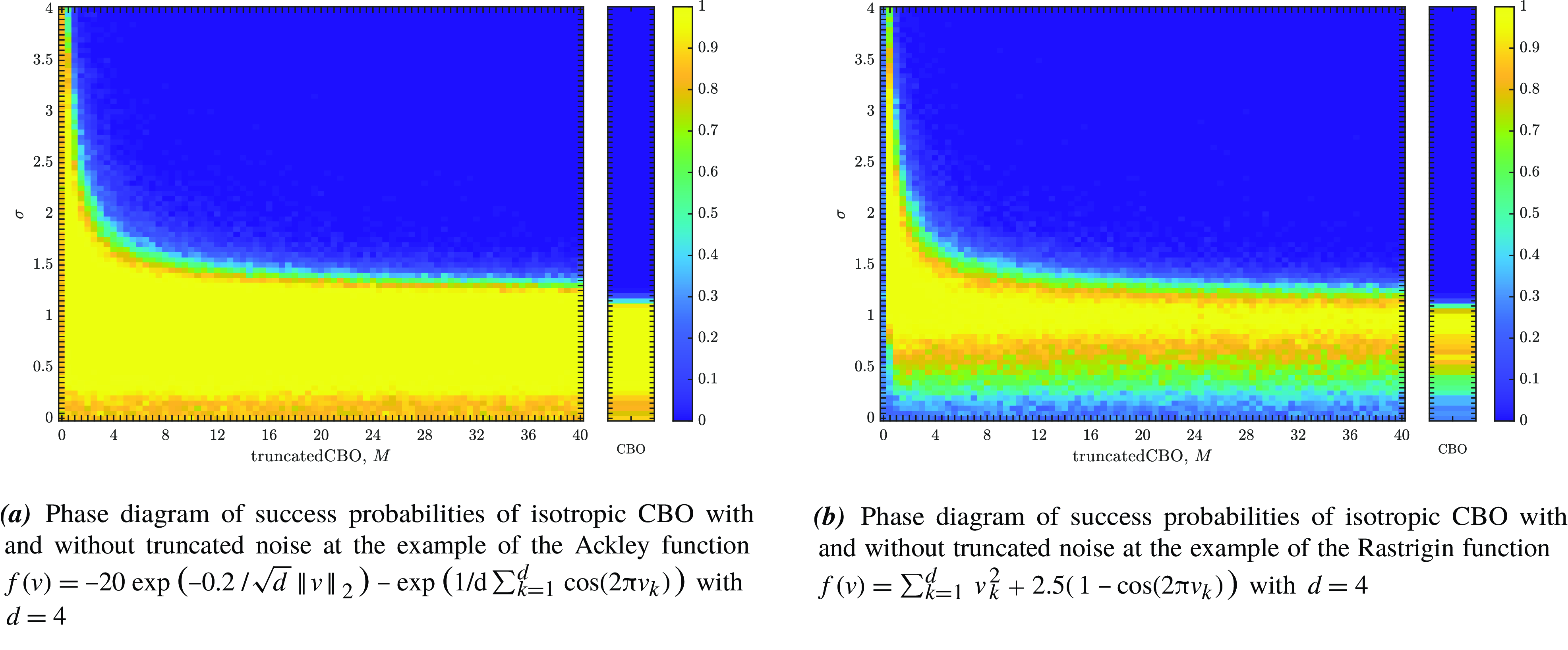
Figure 1. A comparison of the success probabilities of isotropic CBO with (left phase diagrams) and without (right separate columns) truncated noise for different values of the truncation parameter $M$
and the noise level
$M$
and the noise level $\sigma$
. (Note that standard CBO as investigated in [Reference Pinnau, Totzeck, Tse and Martin7, Reference Carrillo, Choi, Totzeck and Tse8, Reference Fornasier, Klock and Riedl10] is retrieved when choosing
$\sigma$
. (Note that standard CBO as investigated in [Reference Pinnau, Totzeck, Tse and Martin7, Reference Carrillo, Choi, Totzeck and Tse8, Reference Fornasier, Klock and Riedl10] is retrieved when choosing $M=\infty$
,
$M=\infty$
, $R=\infty$
and
$R=\infty$
and $v_b=0$
in (1)). In both settings (
a
) and (
b
), the depicted success probabilities are averaged over
$v_b=0$
in (1)). In both settings (
a
) and (
b
), the depicted success probabilities are averaged over $100$
runs and the implemented scheme is given by an Euler–Maruyama discretisation of equation (3) with time horizon
$100$
runs and the implemented scheme is given by an Euler–Maruyama discretisation of equation (3) with time horizon $T=50$
, discrete time step size
$T=50$
, discrete time step size $\Delta t=0.01$
,
$\Delta t=0.01$
, $R=\infty$
,
$R=\infty$
, $v_b=0$
,
$v_b=0$
, $\alpha =10^5$
and
$\alpha =10^5$
and $\lambda =1$
. We use
$\lambda =1$
. We use $N=100$
particles, which are initialised according to
$N=100$
particles, which are initialised according to $\rho _0={\mathcal{N}}((1,\dots,1),2000)$
. In both figures, we plot the success probability of standard CBO (right separate column) and the CBO variant with truncated noise (left phase transition diagram) for different values of the truncation parameter
$\rho _0={\mathcal{N}}((1,\dots,1),2000)$
. In both figures, we plot the success probability of standard CBO (right separate column) and the CBO variant with truncated noise (left phase transition diagram) for different values of the truncation parameter $M$
and the noise level
$M$
and the noise level $\sigma$
, when optimising the Ackley ((
a
)) and Rastrigin ((
b
)) function, respectively. We observe that truncating the noise term (by decreasing
$\sigma$
, when optimising the Ackley ((
a
)) and Rastrigin ((
b
)) function, respectively. We observe that truncating the noise term (by decreasing $M$
) consistently allows for a wider flexibility when choosing the noise level
$M$
) consistently allows for a wider flexibility when choosing the noise level $\sigma$
and thus increasing the likelihood of successfully locating the global minimiser.
$\sigma$
and thus increasing the likelihood of successfully locating the global minimiser.
In conclusion, we observe from Equation (10) that the standard CBO dynamics as described in Equation (9) diverges in the setting $\sigma ^2d\gt 2\lambda$
when considering the Wasserstein-
$\sigma ^2d\gt 2\lambda$
when considering the Wasserstein- $2$
distance
$2$
distance $W_2$
. Contrarily, according to Equation (12), the CBO dynamics with truncated noise as presented in Equation (11) converges with exponential rate towards a neighbourhood of
$W_2$
. Contrarily, according to Equation (12), the CBO dynamics with truncated noise as presented in Equation (11) converges with exponential rate towards a neighbourhood of $v^*$
, with radius
$v^*$
, with radius $\sigma M\sqrt{d}/\sqrt{\lambda }$
. This implies that for a relatively small value of
$\sigma M\sqrt{d}/\sqrt{\lambda }$
. This implies that for a relatively small value of $M$
, the CBO dynamics with truncated noise exhibits greater robustness in relation to the parameter
$M$
, the CBO dynamics with truncated noise exhibits greater robustness in relation to the parameter $\sigma ^2d/\lambda$
. This effect is confirmed numerically in Figure 1.
$\sigma ^2d/\lambda$
. This effect is confirmed numerically in Figure 1.
Remark 1 (Sub-Gaussianity of truncated CBO). An application of Itô’s formula allows to show that, for some $\kappa \gt 0$
,
$\kappa \gt 0$
, $\mathbb{E}\!\left [\exp \!\left (\!\left \| \mkern 1.5mu\overline{\mkern -1.5muY\mkern -1.5mu}\mkern 0mu_t-v^* \right \|_2^2/ \kappa ^2\right )\right ]\lt \infty$
, provided
$\mathbb{E}\!\left [\exp \!\left (\!\left \| \mkern 1.5mu\overline{\mkern -1.5muY\mkern -1.5mu}\mkern 0mu_t-v^* \right \|_2^2/ \kappa ^2\right )\right ]\lt \infty$
, provided $\mathbb{E}\!\left [\exp \!\left (\!\left \| \mkern 1.5mu\overline{\mkern -1.5muY\mkern -1.5mu}\mkern 0mu_0-v^* \right \|_2^2/ \kappa ^2\right )\right ]\lt \infty$
. Thus, by incorporating a truncation in the noise term of the CBO dynamics, we ensure that the resulting distribution
$\mathbb{E}\!\left [\exp \!\left (\!\left \| \mkern 1.5mu\overline{\mkern -1.5muY\mkern -1.5mu}\mkern 0mu_0-v^* \right \|_2^2/ \kappa ^2\right )\right ]\lt \infty$
. Thus, by incorporating a truncation in the noise term of the CBO dynamics, we ensure that the resulting distribution $\mu _t$
exhibits sub-Gaussian behaviour and therefore we enhance the regularity and well-behavedness of the statistics of
$\mu _t$
exhibits sub-Gaussian behaviour and therefore we enhance the regularity and well-behavedness of the statistics of $\mu _t$
. As a consequence, more reliable and stable results when analysing the properties and characteristics of the dynamics are to be expected.
$\mu _t$
. As a consequence, more reliable and stable results when analysing the properties and characteristics of the dynamics are to be expected.
1.2. Contributions
In view of the aforementioned enhanced regularity and well-behavedness of the statistics of CBO with truncated noise compared to standard CBO [Reference Pinnau, Totzeck, Tse and Martin7] together with the numerically observed improved performance as depicted in Figure 1, a rigorous convergence analysis of the implementable CBO algorithm with truncated noise as given in (1) is of theoretical interest. In this work, we provide theoretical guarantees of global convergence of (1) to the global minimiser $v^*$
for possibly non-convex and non-smooth objective functions
$v^*$
for possibly non-convex and non-smooth objective functions $f$
. The approach to analyse the convergence behaviour of the implementable scheme (1) follows a similar route as initiated and explored by the authors of [Reference Carrillo, Choi, Totzeck and Tse8–Reference Fornasier, Klock, Riedl, Laredo, Hidalgo and Babaagba11]. In particular, we first investigate the mean-field behaviour (8) of the system (3). Then, by establishing a quantitative estimate on the mean-field approximation, that is, the proximity of the mean-field system (8) to the interacting particle system (3), we obtain a convergence result for the CBO algorithm (1) with truncated noise. Our proving technique nevertheless differs in crucial parts from the one in [Reference Fornasier, Klock and Riedl10, Reference Fornasier, Klock, Riedl, Laredo, Hidalgo and Babaagba11] as, on the one side, we do take advantage of the truncations, and, on the other side, we require additional technical effort to exploit and deal with the enhanced flexibility of the truncated model. Specifically, the central novelty can be identified in the proof of sub-Gaussianity of the process, see Lemma 8.
$f$
. The approach to analyse the convergence behaviour of the implementable scheme (1) follows a similar route as initiated and explored by the authors of [Reference Carrillo, Choi, Totzeck and Tse8–Reference Fornasier, Klock, Riedl, Laredo, Hidalgo and Babaagba11]. In particular, we first investigate the mean-field behaviour (8) of the system (3). Then, by establishing a quantitative estimate on the mean-field approximation, that is, the proximity of the mean-field system (8) to the interacting particle system (3), we obtain a convergence result for the CBO algorithm (1) with truncated noise. Our proving technique nevertheless differs in crucial parts from the one in [Reference Fornasier, Klock and Riedl10, Reference Fornasier, Klock, Riedl, Laredo, Hidalgo and Babaagba11] as, on the one side, we do take advantage of the truncations, and, on the other side, we require additional technical effort to exploit and deal with the enhanced flexibility of the truncated model. Specifically, the central novelty can be identified in the proof of sub-Gaussianity of the process, see Lemma 8.
1.3. Organisation
In Section 2, we present and discuss our main theoretical contribution about the global convergence of CBO with truncated noise in probability and expectation. Section 3 collects the necessary proof details for this result. In Section 4, we numerically demonstrate the benefits of using truncated noise, before we provide a conclusion of the paper in Section 5. For the sake of reproducible research, in the GitHub repository https://github.com/KonstantinRiedl/CBOGlobalConvergenceAnalysis, we provide the Matlab code implementing CBO with truncated noise.
1.4. Notation
We use $\left \|{\,\cdot \,}\right \|_2$
to denote the Euclidean norm on
$\left \|{\,\cdot \,}\right \|_2$
to denote the Euclidean norm on $\mathbb{R}^d$
. Euclidean balls are denoted as
$\mathbb{R}^d$
. Euclidean balls are denoted as $B_{r}(u) \,:\!=\, \{v \in \mathbb{R}^d\,:\, \|{v-u}\|_2 \leq r\}$
. For the space of continuous functions
$B_{r}(u) \,:\!=\, \{v \in \mathbb{R}^d\,:\, \|{v-u}\|_2 \leq r\}$
. For the space of continuous functions $f\,:\,X\rightarrow Y$
, we write
$f\,:\,X\rightarrow Y$
, we write ${\mathcal{C}}(X,Y)$
, with
${\mathcal{C}}(X,Y)$
, with $X\subset \mathbb{R}^n$
and a suitable topological space
$X\subset \mathbb{R}^n$
and a suitable topological space $Y$
. For an open set
$Y$
. For an open set $X\subset \mathbb{R}^n$
and for
$X\subset \mathbb{R}^n$
and for $Y=\mathbb{R}^m$
, the spaces
$Y=\mathbb{R}^m$
, the spaces ${\mathcal{C}}^k_{c}(X,Y)$
and
${\mathcal{C}}^k_{c}(X,Y)$
and ${\mathcal{C}}^k_{b}(X,Y)$
contain functions
${\mathcal{C}}^k_{b}(X,Y)$
contain functions $f\in{\mathcal{C}}(X,Y)$
that are
$f\in{\mathcal{C}}(X,Y)$
that are $k$
-times continuously differentiable and have compact support or are bounded, respectively. We omit
$k$
-times continuously differentiable and have compact support or are bounded, respectively. We omit $Y$
in the real-valued case. All stochastic processes are considered on the probability space
$Y$
in the real-valued case. All stochastic processes are considered on the probability space $\left (\Omega,\mathscr{F},\mathbb{P}\right )$
. The main objects of study are laws of such processes,
$\left (\Omega,\mathscr{F},\mathbb{P}\right )$
. The main objects of study are laws of such processes, $\rho \in{\mathcal{C}}([0,T],{\mathcal{P}}(\mathbb{R}^d))$
, where the set
$\rho \in{\mathcal{C}}([0,T],{\mathcal{P}}(\mathbb{R}^d))$
, where the set ${\mathcal{P}}(\mathbb{R}^d)$
contains all Borel probability measures over
${\mathcal{P}}(\mathbb{R}^d)$
contains all Borel probability measures over $\mathbb{R}^d$
. With
$\mathbb{R}^d$
. With $\rho _t\in{\mathcal{P}}(\mathbb{R}^d)$
, we refer to a snapshot of such law at time
$\rho _t\in{\mathcal{P}}(\mathbb{R}^d)$
, we refer to a snapshot of such law at time $t$
. Measures
$t$
. Measures $\varrho \in{\mathcal{P}}(\mathbb{R}^d)$
with finite
$\varrho \in{\mathcal{P}}(\mathbb{R}^d)$
with finite $p$
-th moment
$p$
-th moment $\int \|{v}\|_2^p\,d\varrho (v)$
are collected in
$\int \|{v}\|_2^p\,d\varrho (v)$
are collected in ${\mathcal{P}}_p(\mathbb{R}^d)$
. For any
${\mathcal{P}}_p(\mathbb{R}^d)$
. For any $1\leq p\lt \infty$
,
$1\leq p\lt \infty$
, $W_p$
denotes the Wasserstein-
$W_p$
denotes the Wasserstein- $p$
distance between two Borel probability measures
$p$
distance between two Borel probability measures $\varrho _1,\varrho _2\in{\mathcal{P}}_p(\mathbb{R}^d)$
, see, for example, [Reference Ambrosio, Gigli and Savaré46].
$\varrho _1,\varrho _2\in{\mathcal{P}}_p(\mathbb{R}^d)$
, see, for example, [Reference Ambrosio, Gigli and Savaré46]. $\mathbb{E}\!\left [\cdot \right ]$
denotes the expectation.
$\mathbb{E}\!\left [\cdot \right ]$
denotes the expectation.
2. Global convergence of CBO with truncated noise
We now present the main theoretical result of this work about the global convergence of CBO with truncated noise for objective functions that satisfy the following conditions.
Definition 2 (Assumptions). Throughout we are interested in functions ${f} \in{\mathcal{C}}(\mathbb{R}^d)$
, for which
${f} \in{\mathcal{C}}(\mathbb{R}^d)$
, for which
-
A1 there exist $v^*\in \mathbb{R}^d$
such that
${f}(v^*)=\inf _{v\in \mathbb{R}^d}{f}(v)\,=\!:\,\underline{f}$
and
$\underline{\alpha },L_u\gt 0$
such that(13)for any
\begin{align} \sup _{v\in \mathbb{R}^d}\left \| ve^{-\alpha (f(v)-\underline{f})} \right \|_2\,=\!:\,L_u\lt \infty \end{align}
$\alpha \geq \underline{\alpha }$
and any
$v\in \mathbb{R}^d$
,
$v^*\in \mathbb{R}^d$
such that
${f}(v^*)=\inf _{v\in \mathbb{R}^d}{f}(v)\,=\!:\,\underline{f}$
and
$\underline{\alpha },L_u\gt 0$
such that(13)for any
\begin{align} \sup _{v\in \mathbb{R}^d}\left \| ve^{-\alpha (f(v)-\underline{f})} \right \|_2\,=\!:\,L_u\lt \infty \end{align}
$\alpha \geq \underline{\alpha }$
and any
$v\in \mathbb{R}^d$
,
-
A2 there exist
${f}_{\infty },R_0,\nu,L_\nu \gt 0$
such that(14)
\begin{align} \left \|{v-v^*}\right \|_2 &\leq \frac{1}{L_\nu }\big({f}(v)-\underline{f}\big)^{\nu } \quad \text{ for all } v \in B_{R_0}(v^*), \end{align}
(15)
\begin{align}\qquad {f}_{\infty } &\lt{f}(v)-\underline{f}\quad \text{ for all } v \in \big (B_{R_0}(v^*)\big )^c, \end{align}
-
A3 there exist
$L_{\gamma }\gt 0,\gamma \in [0,1]$
such that(16)
\begin{align} \left |{f(v)-f(w)}\right | &\leq L_{\gamma }\!\left(\,\!\left \| v-v^* \right \|_2^{\gamma }+\left \| w-v^* \right \|_2^{\gamma }\right)\left \| v-w \right \|_2 \quad \text{ for all } v, w \in \mathbb{R}^d, \end{align}
(17)
\begin{align} f(v)-\underline{f} &\leq L_{\gamma }\!\left (1+\left \| v-v^* \right \|_2^{1+\gamma }\right ) \quad \text{ for all } v \in \mathbb{R}^d.\qquad \end{align}


A few comments are in order: Condition A1 establishes the existence of a minimiser $v^*$
and requires a certain growth of the function
$v^*$
and requires a certain growth of the function $f$
. Condition A2 ensures that the value of the function
$f$
. Condition A2 ensures that the value of the function $f$
at a point
$f$
at a point $v$
can locally be an indicator of the distance between
$v$
can locally be an indicator of the distance between $v$
and the minimiser
$v$
and the minimiser $v^*$
. This error-bound condition was first introduced in [Reference Fornasier, Klock and Riedl10] under the name inverse continuity condition. It in particular guarantees the uniqueness of the global minimiser
$v^*$
. This error-bound condition was first introduced in [Reference Fornasier, Klock and Riedl10] under the name inverse continuity condition. It in particular guarantees the uniqueness of the global minimiser $v^*$
. Condition A3 sets controllable bounds on the local Lipschitz constant of
$v^*$
. Condition A3 sets controllable bounds on the local Lipschitz constant of $f$
and on the growth of
$f$
and on the growth of $f$
, which is required to be at most quadratic. A similar requirement appears also in [Reference Carrillo, Choi, Totzeck and Tse8, Reference Fornasier, Klock and Riedl10], but there also a quadratic lower bound was imposed.
$f$
, which is required to be at most quadratic. A similar requirement appears also in [Reference Carrillo, Choi, Totzeck and Tse8, Reference Fornasier, Klock and Riedl10], but there also a quadratic lower bound was imposed.
2.1. Main result
We can now state the main result of the paper. Its proof is deferred to Section 3.
Theorem 3. Let ${f} \in{\mathcal{C}}(\mathbb{R}^d)$
satisfy A1, A2 and A3. Moreover, let
${f} \in{\mathcal{C}}(\mathbb{R}^d)$
satisfy A1, A2 and A3. Moreover, let $\rho _0\in{\mathcal{P}}_4(\mathbb{R}^d)$
with
$\rho _0\in{\mathcal{P}}_4(\mathbb{R}^d)$
with $v^*\in \operatorname{supp}(\rho _0)$
. Let
$v^*\in \operatorname{supp}(\rho _0)$
. Let $V^i_{ 0,\Delta t}$
be sampled i.i.d. from
$V^i_{ 0,\Delta t}$
be sampled i.i.d. from $\rho _0$
and denote by
$\rho _0$
and denote by $((V^i_{{k,\Delta t}})_{k=1,\dots,K})_{i=1,\dots,N}$
the iterations generated by the numerical scheme (1). Fix any
$((V^i_{{k,\Delta t}})_{k=1,\dots,K})_{i=1,\dots,N}$
the iterations generated by the numerical scheme (1). Fix any $\epsilon \in \left(0,W_2^2\left (\rho _0,\delta _{v^*}\right )\right )$
, define the time horizon
$\epsilon \in \left(0,W_2^2\left (\rho _0,\delta _{v^*}\right )\right )$
, define the time horizon
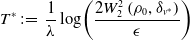 \begin{align*} T^*\,:\!=\,\frac{1}{\lambda }\log \!\left (\frac{2W_2^2\left (\rho _0,\delta _{v^*}\right )}{\epsilon }\right ) \end{align*}
and let $K \in \mathbb{N}$
and
$K \in \mathbb{N}$
and $\Delta t$
satisfy
$\Delta t$
satisfy ${{K\Delta t}}=T^*$
. Moreover, let
${{K\Delta t}}=T^*$
. Moreover, let $R\in \big (\!\left \| v_b-v^* \right \|_2+\sqrt{\epsilon/2},\infty \big )$
,
$R\in \big (\!\left \| v_b-v^* \right \|_2+\sqrt{\epsilon/2},\infty \big )$
, $M\in (0,\infty )$
and
$M\in (0,\infty )$
and $\lambda,\sigma \gt 0$
be such that
$\lambda,\sigma \gt 0$
be such that $\lambda \geq 2\sigma ^2d$
or
$\lambda \geq 2\sigma ^2d$
or $\sigma ^2M^2d=\mathcal{O}(\epsilon )$
. Then, by choosing
$\sigma ^2M^2d=\mathcal{O}(\epsilon )$
. Then, by choosing $\alpha$
sufficiently large and
$\alpha$
sufficiently large and $N\geq \left(16\alpha L_{\gamma }\sigma ^2M^2\right)/\lambda$
, it holds
$N\geq \left(16\alpha L_{\gamma }\sigma ^2M^2\right)/\lambda$
, it holds
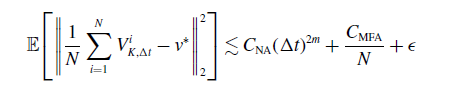 \begin{equation} \mathbb{E}\!\left [\left \| \frac{1}{N} \sum _{i=1}^N V^i_{ K, \Delta t}-v^* \right \|_2^2\right ] \lesssim C_{\textrm{NA}}(\Delta t)^{2m}+\frac{C_{\textrm{MFA}}}{N}+\epsilon \end{equation}
up to a generic constant. Here, $C_{\textrm{NA}}$
depends linearly on the dimension
$C_{\textrm{NA}}$
depends linearly on the dimension $d$
and the number of particles
$d$
and the number of particles $N$
and exponentially on the time horizon
$N$
and exponentially on the time horizon $T^*$
,
$T^*$
, $m$
is the order of accuracy of the numerical scheme (for the Euler–Maruyama scheme
$m$
is the order of accuracy of the numerical scheme (for the Euler–Maruyama scheme $m = 1/2$
), and
$m = 1/2$
), and $C_{\textrm{MFA}} = C_{\textrm{MFA}}(\lambda,\sigma,d,\alpha,L_{\nu },\nu,L_{\gamma },L_u,T^*,R,v_b,v^*,M)$
.
$C_{\textrm{MFA}} = C_{\textrm{MFA}}(\lambda,\sigma,d,\alpha,L_{\nu },\nu,L_{\gamma },L_u,T^*,R,v_b,v^*,M)$
.
Remark 4. In the statement of Theorem 3, the parameters $R$
and
$R$
and $v_b$
play a crucial role. We already mentioned how they can be chosen in an example after Equation (5). The role of these parameters is bolstered in particular in the proof of Theorem 3, where it is demonstrated that, by selecting a sufficiently large
$v_b$
play a crucial role. We already mentioned how they can be chosen in an example after Equation (5). The role of these parameters is bolstered in particular in the proof of Theorem 3, where it is demonstrated that, by selecting a sufficiently large $\alpha$
depending on
$\alpha$
depending on $R$
and
$R$
and $v_b$
, the dynamics (8) can be set equal to
$v_b$
, the dynamics (8) can be set equal to
 \begin{equation*} d \overline {V}_t=-\lambda \!\left (\overline {V}_t-\mathcal {P}_{v^*,\delta }(v_\alpha (\rho _t))\right )dt+\sigma \!\left (\left \|\overline {V}_t-v_{\alpha }(\rho _t)\right \|_2\wedge M\right )d B_t, \end{equation*}
where $\delta$
represents a small value. For the dynamics (3), we can analogously establish its equivalence to
$\delta$
represents a small value. For the dynamics (3), we can analogously establish its equivalence to
 \begin{equation*} d V^i_t=-\lambda \!\left (V^i_t-\mathcal {P}_{v^*,\delta }\left(v_\alpha \!\left(\widehat {\rho }_t^N\right)\right)\right )dt+\sigma \!\left (\left \| V^i_t-v_{\alpha }\left(\widehat {\rho }^N_t\right) \right \|_2\wedge M\right )dB^i_t,\quad \text {$i=1,\dots,N$}, \end{equation*}
with high probability, contingent upon the selection of sufficiently large values for both $\alpha$
and
$\alpha$
and $N$
.
$N$
.
Remark 5. The convergence result in the form of Theorem 3 obtained in this work differs from the one presented in [Reference Fornasier, Klock and Riedl10, Theorem 14] in the sense that we obtain convergence is in expectation, while in [Reference Fornasier, Klock and Riedl10] convergence with high probability is established. This distinction arises from the truncation of the noise term employed in our algorithm.
3. Proof details for section 2
3.1. Well-posedness of equations (1) and (3)
With the projection map ${\mathcal{P}}_{v_b,R}$
being
${\mathcal{P}}_{v_b,R}$
being $1$
-Lipschitz, existence and uniqueness of strong solutions to the SDEs (1) and (3) are assured by essentially analogous proofs as in [Reference Carrillo, Choi, Totzeck and Tse8, Theorems 2.1, 3.1 and 3.2]. The details shall be omitted. Let us remark, however, that due to the presence of the truncation and the projection map, we do not require the function
$1$
-Lipschitz, existence and uniqueness of strong solutions to the SDEs (1) and (3) are assured by essentially analogous proofs as in [Reference Carrillo, Choi, Totzeck and Tse8, Theorems 2.1, 3.1 and 3.2]. The details shall be omitted. Let us remark, however, that due to the presence of the truncation and the projection map, we do not require the function $f$
to be bounded from above or exhibit quadratic growth outside a ball, as required in [Reference Carrillo, Choi, Totzeck and Tse8, Theorems 2.1, 3.1 and 3.2].
$f$
to be bounded from above or exhibit quadratic growth outside a ball, as required in [Reference Carrillo, Choi, Totzeck and Tse8, Theorems 2.1, 3.1 and 3.2].
3.2. Proof details for theorem 3
Remark 6. Since adding some constant offset to $f$
does not affect the dynamics of Equations (3) and (8), we will assume
$f$
does not affect the dynamics of Equations (3) and (8), we will assume $\underline{f}=0$
in the proofs for simplicity but without loss of generality.
$\underline{f}=0$
in the proofs for simplicity but without loss of generality.
Let us first provide a sketch of the proof of Theorem 3. For the approximation error (18), we have the error decomposition
 \begin{equation} \begin{aligned} \mathbb{E}\!\left [\left \| \frac{1}{N} \sum _{i=1}^N V^i_{ K, \Delta t}-v^* \right \|_2^2\right ] &\lesssim \underbrace{\mathbb{E}\!\left [\left \| \frac{1}{N} \sum _{i=1}^N \left (V^i_{ K, \Delta t}-V_{T^*}^i\right ) \right \|_2^2\right ]}_{I}+\underbrace{\mathbb{E}\!\left [\left \| \frac{1}{N} \sum _{i=1}^N \left (V_{T^*}^i-\overline{V}_{T^*}^i\right ) \right \|_2^2\right ]}_{II}\\ &\qquad \qquad \quad +\underbrace{\mathbb{E}\!\left [\left \| \frac{1}{N} \sum _{i=1}^N \overline{V}_{T^*}^i-v^* \right \|_2^2\right ]}_{III}, \end{aligned} \end{equation}
where $\big(\big(\overline{V}_t^i\big)_{t\geq 0}\big)_{i=1,\dots,N}$
denote
$\big(\big(\overline{V}_t^i\big)_{t\geq 0}\big)_{i=1,\dots,N}$
denote $N$
independent copies of the mean-field process
$N$
independent copies of the mean-field process $\big(\overline{V}_t\big)_{t\geq 0}$
satisfying Equation (8).
$\big(\overline{V}_t\big)_{t\geq 0}$
satisfying Equation (8).
In what follows, we investigate each of the three term separately. Term $I$
can be bounded by
$I$
can be bounded by $C_{\textrm{NA}}\!\left (\Delta t\right )^{2m}$
using classical results on the convergence of numerical schemes for SDEs, as mentioned for instance in [Reference Platen43]. The second and third terms, respectively, are analysed in separate subsections, providing detailed explanations and bounds for each of the two terms
$C_{\textrm{NA}}\!\left (\Delta t\right )^{2m}$
using classical results on the convergence of numerical schemes for SDEs, as mentioned for instance in [Reference Platen43]. The second and third terms, respectively, are analysed in separate subsections, providing detailed explanations and bounds for each of the two terms $II$
and
$II$
and $III$
.
$III$
.
Before doing so, let us provide a concise guide for reading the proofs. As the proofs are quite technical, we start for reader’s convenience by presenting the main building blocks of the result first and collect the more technical steps in subsequent lemmas. This arrangement should hopefully allow to grasp the structure of the proof more easily and to dig deeper into the details along with the reading.
3.2.1. Upper bound for the second term in (19)
For Term $II$
of the error decomposition (19), we have the following upper bound.
$II$
of the error decomposition (19), we have the following upper bound.
Proposition 7. Let ${f} \in{\mathcal{C}}(\mathbb{R}^d)$
satisfy A1, A2 and A3. Moreover, let
${f} \in{\mathcal{C}}(\mathbb{R}^d)$
satisfy A1, A2 and A3. Moreover, let $R$
and
$R$
and $M$
be finite such that
$M$
be finite such that $R\geq \left \| v_b-v^* \right \|_2$
and let
$R\geq \left \| v_b-v^* \right \|_2$
and let $N\geq (16\alpha L_{\gamma }\sigma ^2M^2)/\lambda$
. Then, we have
$N\geq (16\alpha L_{\gamma }\sigma ^2M^2)/\lambda$
. Then, we have
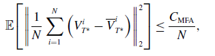 \begin{equation} \mathbb{E}\!\left [\left \| \frac{1}{N} \sum _{i=1}^N \left (V_{T^*}^i-\overline{V}_{T^*}^i\right ) \right \|_2^2\right ]\leq \frac{C_{\textrm{MFA}}}{N}, \end{equation}
where $C_{\textrm{MFA}} = C_{\textrm{MFA}}(\lambda,\sigma,d,\alpha,L_{\nu },\nu,L_{\gamma },L_u,T^*,R,v_b,v^*,M)$
.
$C_{\textrm{MFA}} = C_{\textrm{MFA}}(\lambda,\sigma,d,\alpha,L_{\nu },\nu,L_{\gamma },L_u,T^*,R,v_b,v^*,M)$
.
Proof. By a synchronous coupling, we have
 \begin{align*} d \overline{V}^i_t &=-\lambda \!\left (\overline{V}^i_t-\mathcal{P}_{v_b,R}\!\left (v_{\alpha }(\rho _t)\right )\right )dt+\sigma \!\left (\left \| \overline{V}^i_t-v_{\alpha }(\rho _t) \right \|_2\wedge M\right )d B^i_t,\\ d{V}^i_t &=-\lambda \!\left ({V}^i_t-\mathcal{P}_{v_b,R}\!\left (v_{\alpha }\!\left(\widehat{\rho }_t^N\right)\right )\right )dt+\sigma \!\left (\left \| \overline{V}^i_t-v_{\alpha }\!\left(\widehat \rho ^{\,N}_{t}\right) \right \|_2\wedge M\right )d B^i_t, \end{align*}
with coinciding Brownian motions. Moreover, recall that $\textrm{Law}\big(\overline{V}_t^i\big)=\rho _t$
and
$\textrm{Law}\big(\overline{V}_t^i\big)=\rho _t$
and $\widehat \rho ^{\,N}_{t}={1}/{N}\sum _{i=1}^N\delta _{V_t^i}$
. By Itô’s formula, we then have
$\widehat \rho ^{\,N}_{t}={1}/{N}\sum _{i=1}^N\delta _{V_t^i}$
. By Itô’s formula, we then have
 \begin{equation} \begin{aligned} d\!\left \| \overline{V}^i_t-V_t^i \right \|_2^2& =\Big ({-}2\lambda \!\left \lt \overline{V}^i_t-V_t^i, \left (\overline{V}^i_t-V_t^i\right )-\left (\mathcal{P}_{v_b,R}\!\left (v_{\alpha }(\rho _t)\right )-\mathcal{P}_{v_b,R}\!\left (v_{\alpha }\!\left(\widehat{\rho }_t^N\right)\right )\right ) \right \gt \\ &\quad \,+\sigma ^2d\!\left (\left \| \overline{V}^i_t-v_{\alpha }(\rho _t) \right \|_2\wedge M-\left \| V_t^i-{v}_{\alpha }\!\left(\widehat \rho ^{\,N}_{t}\right) \right \|_2\wedge M\right )^2\Big )\,dt\\ &\quad \,+2\sigma \!\left (\left \| \overline{V}^i_t-v_{\alpha }(\rho _t) \right \|_2\wedge M-\left \| V_t^i-{v}_{\alpha }\!\left(\widehat \rho ^{\,N}_{t}\right) \right \|_2\wedge M\right )\left (\overline{V}^i_t-V_t^i\right )^{\top }dB^i_t, \end{aligned} \end{equation}
and after taking the expectation on both sides
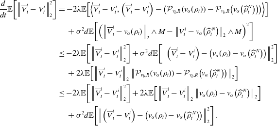 \begin{equation} \begin{aligned} \frac{d}{dt}\mathbb{E}\!\left [\left \| \overline{V}^i_t-V_t^i \right \|_2^2\right ]&=-2\lambda \mathbb{E}\!\left [\left \lt \overline{V}^i_t-V_t^i, \left (\overline{V}^i_t-V_t^i\right )-\left (\mathcal{P}_{v_b,R}\!\left (v_{\alpha }(\rho _t)\right )-\mathcal{P}_{v_b,R}\!\left (v_{\alpha }\!\left(\widehat{\rho }_t^N\right)\right )\right ) \right \gt \right ]\\ &\quad \,+\sigma ^2d\mathbb{E}\!\left [\left (\left \| \overline{V}^i_t-v_{\alpha }(\rho _t) \right \|_2\wedge M-\left \| V_t^i-{v}_{\alpha }\!\left(\widehat \rho ^{\,N}_{t}\right) \right \|_2\wedge M\right )^2\right ]\\ &\leq -2\lambda \mathbb{E}\!\left [\left \| \overline{V}^i_t-V_t^i \right \|_2^2\right ]+\sigma ^2d\mathbb{E}\!\left [\left \| \left (\overline{V}^i_t-V_t^i\right )-\left (v_{\alpha }(\rho _t)-{v}_{\alpha }\!\left(\widehat \rho ^{\,N}_{t}\right)\right ) \right \|_2^2\right ]\\ &\quad \,+2\lambda \mathbb{E}\!\left [\left \| \overline{V}^i_t-V_t^i \right \|_2\left \| \mathcal{P}_{v_b,R}\!\left (v_{\alpha }(\rho _t)\right )-\mathcal{P}_{v_b,R}\!\left (v_{\alpha }\!\left(\widehat{\rho }_t^N\right)\right ) \right \|_2\right ]\\ &\leq -2\lambda \mathbb{E}\!\left [\left \| \overline{V}^i_t-V_t^i \right \|_2^2\right ]+2\lambda \mathbb{E}\!\left [\left \| \overline{V}^i_t-V_t^i \right \|_2\left \| v_{\alpha }(\rho _t)-{v}_{\alpha }\!\left(\widehat \rho ^{\,N}_{t}\right) \right \|_2\right ]\\ &\quad \,+\sigma ^2d\mathbb{E}\!\left [\left \| \left (\overline{V}^i_t-V_t^i\right )-\left (v_{\alpha }(\rho _t)-{v}_{\alpha }\!\left(\widehat \rho ^{\,N}_{t}\right)\right ) \right \|_2^2\right ]. \end{aligned} \end{equation}
Here, let us remark that the last (stochastic) term in (21) disappears after taking the expectation. This is due to $\mathbb{E}\!\left [\left \| \overline{V}_t^i-V_t^i \right \|_2^2\right ]\lt \infty$
, which can be derived from Lemma 8 after noticing that Lemma 8 also holds for processes
$\mathbb{E}\!\left [\left \| \overline{V}_t^i-V_t^i \right \|_2^2\right ]\lt \infty$
, which can be derived from Lemma 8 after noticing that Lemma 8 also holds for processes $V_t^i$
. Since by Young’s inequality, it holds
$V_t^i$
. Since by Young’s inequality, it holds
 \begin{equation*} 2\lambda \mathbb {E}\!\left [\left \| \overline {V}^i_t-V_t^i \right \|_2\left \| v_{\alpha }(\rho _t)-{v}_{\alpha }\!\left(\widehat \rho ^{\,N}_{t}\right) \right \|_2\right ]\leq \lambda \!\left (\frac {\mathbb {E}\!\left [\left \| \overline {V}^i_t-V_t^i \right \|_2^2\right ]}{2}+2\mathbb {E}\!\left [\left \| v_{\alpha }(\rho _t)-{v}_{\alpha }\!\left(\widehat \rho ^{\,N}_{t}\right) \right \|_2^2\right ]\right ), \end{equation*}
and
 \begin{equation*} \mathbb {E}\!\left [\left \| \left (\overline {V}^i_t-V_t^i\right )-\left (v_{\alpha }(\rho _t)-{v}_{\alpha }\!\left(\widehat \rho ^{\,N}_{t}\right)\right ) \right \|_2^2\right ]\leq 2 \mathbb {E}\!\left [\left \| \overline {V}^i_t-V_t^i \right \|_2^2+\left \| v_{\alpha }(\rho _t)-{v}_{\alpha }\!\left(\widehat \rho ^{\,N}_{t}\right) \right \|_2^2\right ], \end{equation*}
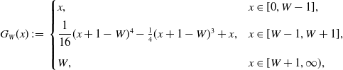
we obtain
 \begin{equation} \frac{d}{dt}\mathbb{E}\!\left [\Big \| \overline{V}^i_t-V_t^i \Big\|_2^2\right ] \leq \left ({-}\frac{3\lambda }{2}+2\sigma ^2d\right )\mathbb{E}\!\left [\left \| \overline{V}^i_t-V_t^i \right \|_2^2\right ] +2\!\left (\lambda +\sigma ^2d\right )\mathbb{E}\!\left [\left \| v_{\alpha }(\rho _t)-{v}_{\alpha }\!\left(\widehat \rho ^{\,N}_{t}\right) \right \|_2^2\right ] \end{equation}
after inserting the former two inequalities into Equation (22). For the term $\mathbb{E}\!\left [\left \| v_{\alpha }(\rho _t)-{v}_{\alpha }\!\left(\widehat \rho ^{\,N}_{t}\right) \right \|_2^2\right ]$
, we can decompose
$\mathbb{E}\!\left [\left \| v_{\alpha }(\rho _t)-{v}_{\alpha }\!\left(\widehat \rho ^{\,N}_{t}\right) \right \|_2^2\right ]$
, we can decompose
 \begin{equation} \begin{aligned} \mathbb{E}\!\left [\left \| v_{\alpha }(\rho _t)-{v}_{\alpha }\!\left(\widehat \rho ^{\,N}_{t}\right) \right \|_2^2\right ]\leq 2\mathbb{E}\!\left [\left \| v_{\alpha }(\rho _t)-{v}_{\alpha }\!\left(\bar{\rho }^N_t\right) \right \|_2^2\right ]+2\mathbb{E}\!\left [\left \|{v}_{\alpha }\!\left(\bar{\rho }^N_t\right)-{v}_{\alpha }\!\left(\widehat \rho ^{\,N}_{t}\right) \right \|_2^2\right ], \end{aligned} \end{equation}
where we denote
 \begin{equation*} \bar {\rho }^N_t=\frac {1}{N}\sum _{i=1}^N\delta _{\mkern 1.5mu\overline {\mkern -1.5muV\mkern -1.5mu}\mkern 0mu_t^i}. \end{equation*}
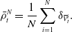
For the first term in Equation (24), by Lemma 11, we have
 \begin{equation*} \mathbb {E}\!\left [\left \| v_{\alpha }(\rho _t)-{v}_{\alpha }\!\left(\bar {\rho }^N_t\right) \right \|_2^2\right ]\leq {C_0}\frac {1}{N} \end{equation*}
for some constant $C_0$
depending on
$C_0$
depending on $\lambda,\sigma,d,\alpha,L_{\gamma },L_u,T^*,R,v_b,v^*$
and
$\lambda,\sigma,d,\alpha,L_{\gamma },L_u,T^*,R,v_b,v^*$
and $M$
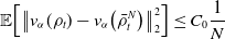
. For the second term in Equation (24), by combining [Reference Carrillo, Choi, Totzeck and Tse8, Lemma 3.2] and Lemma 8, we obtain
$M$
. For the second term in Equation (24), by combining [Reference Carrillo, Choi, Totzeck and Tse8, Lemma 3.2] and Lemma 8, we obtain
 \begin{equation*} \mathbb {E}\!\left [\left \| {v}_{\alpha }\!\left(\bar {\rho }^N_t\right)-{v}_{\alpha }\!\left(\widehat \rho ^{\,N}_{t}\right) \right \|_2^2\right ]\leq C_1\frac {1}{N}\sum _{i=1}^N\mathbb {E}\!\left [\left \| \overline {V}^i_t-V_t^i \right \|_2^2\right ], \end{equation*}
for some constant $C_1$
depending on
$C_1$
depending on $\lambda,\sigma,d,\alpha,L_u,R$
and
$\lambda,\sigma,d,\alpha,L_u,R$
and $M$
. Combining these estimates, we conclude
$M$
. Combining these estimates, we conclude
 \begin{equation*} \begin{aligned} \frac{d}{dt}\frac{1}{N}\sum _{i=1}^N\mathbb{E}\!\left [\left \| \overline{V}^i_t-V_t^i \right \|_2^2\right ]&\leq \left ({-}\frac{3\lambda }{2}+2\sigma ^2d+4C_1\left (\lambda +\sigma ^2 d\right )\right )\frac{1}{N}\sum _{i=1}^N\mathbb{E}\!\left [\left \| \overline{V}^i_t-V_t^i \right \|_2^2\right ]\\ &\quad \,+ 4\!\left (\lambda +\sigma ^2 d\right )C_0\frac{1}{N}. \end{aligned} \end{equation*}
After an application of Grönwall’s inequality and noting that $\overline{V}^i_0=V^i_0$
for all
$\overline{V}^i_0=V^i_0$
for all $i=1,\dots,N$
, we have
$i=1,\dots,N$
, we have
 \begin{equation} \begin{aligned} \frac{1}{N}\sum _{i=1}^N\mathbb{E}\!\left [\left \| \overline{V}^i_t-V_t^i \right \|_2^2\right ]&\leq 4\!\left (\lambda +\sigma ^2 d\right )\frac{C_0}{N}te^{\left ({-}\frac{3\lambda }{2}+2\sigma ^2d+4C_1\left(\lambda +\sigma ^2 d\right)\right )t}. \end{aligned} \end{equation}
for any $t\in [0,T^*]$
. Finally, by Jensen’s inequality and letting
$t\in [0,T^*]$
. Finally, by Jensen’s inequality and letting $t=T^*$
, we have
$t=T^*$
, we have
 \begin{equation} \mathbb{E}\!\left [\left \| \frac{1}{N} \sum _{i=1}^N \left (V_{T^*}^i-\overline{V}_{T^*}^i\right ) \right \|_2^2\right ]\leq \frac{C_{\textrm{MFA}}}{N}, \end{equation}
where the constant $C_{\textrm{MFA}}$
depends on
$C_{\textrm{MFA}}$
depends on $\lambda,\sigma,d,\alpha,L_u,L_{\gamma },T^*,R,v_b,v^*$
and
$\lambda,\sigma,d,\alpha,L_u,L_{\gamma },T^*,R,v_b,v^*$
and $M$
.
$M$
.
In the next lemma, we show that the distribution of $\overline{V}_t$
is sub-Gaussian.
$\overline{V}_t$
is sub-Gaussian.
Lemma 8. Let $R$
and
$R$
and $M$
be finite with
$M$
be finite with $R\geq \left \| v_b-v^* \right \|_2$
. For any
$R\geq \left \| v_b-v^* \right \|_2$
. For any $ \kappa \gt 0$
, let
$ \kappa \gt 0$
, let $N$
satisfy
$N$
satisfy $N\geq{\left(4 \sigma ^2 M^2\right)}/{\left(\lambda \kappa ^2\right)}$
. Then, provided that
$N\geq{\left(4 \sigma ^2 M^2\right)}/{\left(\lambda \kappa ^2\right)}$
. Then, provided that $\mathbb{E}\!\left [\exp \!\left({\sum _{i=1}^N\big\| \overline{V}^i_0-v^* \big\|_2^2}/{\left(N \kappa ^2\right)}\right)\right ]\lt \infty$
, it holds
$\mathbb{E}\!\left [\exp \!\left({\sum _{i=1}^N\big\| \overline{V}^i_0-v^* \big\|_2^2}/{\left(N \kappa ^2\right)}\right)\right ]\lt \infty$
, it holds
 \begin{equation} C_{ \kappa }\,:\!=\, \sup _{t\in [0,T^*]}\mathbb{E}\!\left [\exp \!\left (\frac{\sum _{i=1}^N\left \| \mkern 1.5mu\overline{\mkern -1.5muV\mkern -1.5mu}\mkern 0mu^i_t-v^* \right \|_2^2}{N \kappa ^2}\right )\right ] \lt \infty, \end{equation}
where $C_{ \kappa }$
depends on
$C_{ \kappa }$
depends on $ \kappa,\lambda,\sigma,d,R,M$
and
$ \kappa,\lambda,\sigma,d,R,M$
and $T^*$
, and where
$T^*$
, and where
 \begin{equation*} d \overline {V}^i_t =-\lambda \!\left (\overline {V}^i_t-\mathcal {P}_{v_b,R}\left (v_{\alpha }(\rho _t)\right )\right )dt+\sigma \!\left (\left \| \overline {V}^i_t-v_{\alpha }(\rho _t) \right \|_2\wedge M\right )d B^i_t \end{equation*}
for $i=1,\dots,N$
with
$i=1,\dots,N$
with $B^i_t$
being independent to each other and
$B^i_t$
being independent to each other and $\textrm{Law}\big(\overline{V}_t^i\big)=\rho _t$
.
$\textrm{Law}\big(\overline{V}_t^i\big)=\rho _t$
.
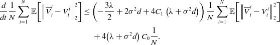
Proof. To apply Itô’s formula, we need to truncate the function $\exp \!\left({\left \| v \right \|_2^2}/{ \kappa ^2}\right)$
from above. For this, define for
$\exp \!\left({\left \| v \right \|_2^2}/{ \kappa ^2}\right)$
from above. For this, define for $W\gt 0$
the function
$W\gt 0$
the function
 \begin{equation*} G_W(x)\,:\!=\,\begin {cases} x,& x\in [0,W-1],\\[5pt] \dfrac {1}{16}(x+1-W)^4-\frac {1}{4}(x+1-W)^3+x,&x\in [W-1,W+1],\\[10pt] W,&x\in [W+1,\infty), \end {cases} \end{equation*}
It is easy to verify that $G_W$
is a
$G_W$
is a $\mathcal{C}^2$
approximation of the function
$\mathcal{C}^2$
approximation of the function $x\wedge W$
satisfying
$x\wedge W$
satisfying $ G_W\in \mathcal{C}^2(\mathbb{R}^+)$
,
$ G_W\in \mathcal{C}^2(\mathbb{R}^+)$
, $G_W(x)\leq x\wedge W$
,
$G_W(x)\leq x\wedge W$
, $ G_W^{\prime }\in [0,1]$
and
$ G_W^{\prime }\in [0,1]$
and $G_W^{\prime \prime }\leq 0$
.
$G_W^{\prime \prime }\leq 0$
.
Since $G_{W,N, \kappa }(t)\,:\!=\,\exp \!\left(G_W\!\left(\sum _{i=1}^N\big\| \overline{V}^i_t-v^* \big\|_2^2/N\right)/{ \kappa ^2}\right)$
is upper-bounded, we can apply Itô’s formula to it. We abbreviate
$G_{W,N, \kappa }(t)\,:\!=\,\exp \!\left(G_W\!\left(\sum _{i=1}^N\big\| \overline{V}^i_t-v^* \big\|_2^2/N\right)/{ \kappa ^2}\right)$
is upper-bounded, we can apply Itô’s formula to it. We abbreviate $G_W^{\prime }\,:\!=\,G_W^{\prime }\left(\!\sum _{i=1}^N\big\| \overline{V}_t^i -v^* \big\|_2^2/N\right)$
and
$G_W^{\prime }\,:\!=\,G_W^{\prime }\left(\!\sum _{i=1}^N\big\| \overline{V}_t^i -v^* \big\|_2^2/N\right)$
and $G_W^{\prime \prime }\,:\!=\,G_W^{\prime \prime }\left(\!\sum _{i=1}^N\big\| \overline{V}_t^i \big\|_2^2/N\right)$
in what follows. With the notation
$G_W^{\prime \prime }\,:\!=\,G_W^{\prime \prime }\left(\!\sum _{i=1}^N\big\| \overline{V}_t^i \big\|_2^2/N\right)$
in what follows. With the notation $Y_t\,:\!=\,\left (\big(\overline{V}_t^1\big)^{\top },\cdots,\big(\overline{V}_t^N\big)^{\top }\right )^{\top }$
, the
$Y_t\,:\!=\,\left (\big(\overline{V}_t^1\big)^{\top },\cdots,\big(\overline{V}_t^N\big)^{\top }\right )^{\top }$
, the $Nd$
-dimensional process
$Nd$
-dimensional process $Y_t$
satisfies
$Y_t$
satisfies $ dY_t=-\lambda \big (Y_t-\overline{\mathcal{P}_{v_b,R}(\rho _t)}\big )\,dt+\mathcal{M}dB_t$
, where
$ dY_t=-\lambda \big (Y_t-\overline{\mathcal{P}_{v_b,R}(\rho _t)}\big )\,dt+\mathcal{M}dB_t$
, where $\overline{\mathcal{P}_{v_b,R}(\rho _t)}=\left ({\mathcal{P}_{v_b,R}(\rho _t)}^{\top },\ldots,{\mathcal{P}_{v_b,R}(\rho _t)}^{\top }\right )^{\top }$
,
$\overline{\mathcal{P}_{v_b,R}(\rho _t)}=\left ({\mathcal{P}_{v_b,R}(\rho _t)}^{\top },\ldots,{\mathcal{P}_{v_b,R}(\rho _t)}^{\top }\right )^{\top }$
, $\mathcal{M}=\operatorname{diag}\!\left (\mathcal{M}_1,\ldots,\mathcal{M}_N\right )$
with
$\mathcal{M}=\operatorname{diag}\!\left (\mathcal{M}_1,\ldots,\mathcal{M}_N\right )$
with $\mathcal{M}_i=\sigma \big\| \overline{V}^i_t-v_\alpha \!\left (\rho _t\right ) \big\|_2\wedge M \textrm{I}_{d}$
and
$\mathcal{M}_i=\sigma \big\| \overline{V}^i_t-v_\alpha \!\left (\rho _t\right ) \big\|_2\wedge M \textrm{I}_{d}$
and $B_t$
the
$B_t$
the $Nd$
-dimensional Brownian motion. We then have
$Nd$
-dimensional Brownian motion. We then have $G_{W,N, \kappa }(t)=\exp \!\left (G_W\big (\!\left \| Y_t \right \|_2^2/N\big )/ \kappa ^2\right )$
and
$G_{W,N, \kappa }(t)=\exp \!\left (G_W\big (\!\left \| Y_t \right \|_2^2/N\big )/ \kappa ^2\right )$
and
 \begin{equation} \begin{aligned} d G_{W,N, \kappa }(t)&= \sum _{i=1}^N\nabla _{Y_t}G_{W,N, \kappa }(t) dY_t+\frac{1}{2}\operatorname{tr}\!\left (\mathcal{M}\nabla _{Y_t,Y_t}^2 G_{W,N, \kappa }(t) \mathcal{M}\right )dt\\ &=G_{W,N, \kappa }(t)\frac{G_W^{\prime }}{ \kappa ^2}\sum _{i=1}^N\left (2\frac{\overline{V}^i_t-v^*}{N}\right )^{\top }d\overline{V}^i_t\\ &\quad \,+\frac{1}{2}G_{W,N, \kappa }(t)\sum _{i=1}^N\left (G_W^{\prime }\frac{2d}{N \kappa ^2}+G_W^{\prime \prime }\frac{4\big\| \overline{V}^i_t-v^* \big\|_2^2}{N^2 \kappa ^2}\right .\\ &\quad \,\left .+\left (G_W^{\prime }\right )^2\frac{4\big\| \overline{V}^i_t-v^* \big\|_2^2}{N^2 \kappa ^4}\right )\left (\sigma \!\left \| \overline{V}^i_t-v_\alpha \left (\rho _t\right ) \right \|_2\wedge M\right )^2dt.\\ \end{aligned} \end{equation}
The first term on the right-hand side of (28) can be expanded as
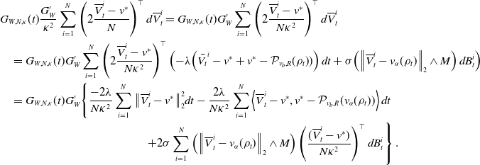 \begin{equation} \begin{aligned} &G_{W,N, \kappa }(t)\frac{G_W^{\prime }}{ \kappa ^2}\sum _{i=1}^N\left (2\frac{\overline{V}^i_t-v^*}{N}\right )^{\top }d\overline{V}^i_t =G_{W,N, \kappa }(t)G_W^{\prime }\sum _{i=1}^N\left (2\frac{\overline{V}^i_t-v^*}{N \kappa ^2}\right )^{\top }d\overline{V}^i_t\\ &\quad =G_{W,N, \kappa }(t)G_W^{\prime }\sum _{i=1}^N\left (2\frac{\overline{V}^i_t-v^*}{N \kappa ^2}\right )^{\top }\left ({-}\lambda \!\left (\bar{V_t}^i-v^*+{v^*-\mathcal{P}_{v_b,R}(\rho _t)})\right )dt+\sigma \!\left (\left \| \overline{V}^i_t-v_{\alpha }(\rho _t) \right \|_2\wedge M\right )d B^i_t\right )\\ &\quad = G_{W,N, \kappa }(t)G_W^{\prime }\!\left \{\frac{-2\lambda }{N \kappa ^2}\sum _{i=1}^N\big\| \overline{V}_t^i-v^* \big\|_2^2dt-\frac{2\lambda }{N \kappa ^2}\sum _{i=1}^N\left \lt \overline{V}_t^i-v^*, v^*-\mathcal{P}_{v_b,R}(v_\alpha (\rho _t)) \right \gt dt \right. \\ & \phantom{XXXXXXXXXXXXXXXXXXX}\;\;\,\left. +2\sigma \sum _{i=1}^N \left (\left \| \overline{V}^i_t-v_{\alpha }(\rho _t) \right \|_2\wedge M\right )\left (\frac{(\overline{V}^i_t-v^*)}{N \kappa ^2}\right )^{\top }d B^i_t \right \}. \end{aligned} \end{equation}
Notice additionally that
 \begin{equation} \left \lt \overline{V}_t^i-v^*, v^*-\mathcal{P}_{v_b,R}(v_\alpha (\rho _t)) \right \gt \leq \big\| \overline{V}_t^i-v^* \big\|_2\left \| v^*-\mathcal{P}_{v_b,R}(v_\alpha (\rho _t)) \right \|_2 \leq 2 R \big\| \overline{V}_t^i-v^* \big\|_2 \end{equation}
as $v^*$
and
$v^*$
and $\mathcal{P}_{v_b,R}(v_\alpha (\rho _t))$
belong to the same ball
$\mathcal{P}_{v_b,R}(v_\alpha (\rho _t))$
belong to the same ball $B_R(v_b)$
around
$B_R(v_b)$
around $v_b$
of radius
$v_b$
of radius $R$
. Similarly, we can expand the coefficient of the second term. According to the properties
$R$
. Similarly, we can expand the coefficient of the second term. According to the properties $G_W^{\prime }\in [0,1]$
and
$G_W^{\prime }\in [0,1]$
and $G_W^{\prime \prime }\leq 0$
, we can bound it from above yielding
$G_W^{\prime \prime }\leq 0$
, we can bound it from above yielding
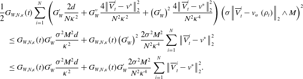 \begin{equation} \begin{aligned} &\frac{1}{2}G_{W,N, \kappa }(t)\sum _{i=1}^N\left (G_W^{\prime }\frac{2d}{N \kappa ^2}+G_W^{\prime \prime }\frac{4\big\| \overline{V}^i_t-v^* \big\|_2^2}{N^2 \kappa ^2}+\left (G_W^{\prime }\right )^2\frac{4\big\| \overline{V}^i_t-v^* \big\|_2^2}{N^2 \kappa ^4}\right )\left (\sigma \!\left \| \overline{V}^i_t-v_\alpha \left (\rho _t\right ) \right \|_2\wedge M\right )^2\\ &\quad \leq G_{W,N, \kappa }(t)G_W^{\prime }\frac{\sigma ^2M^2d}{ \kappa ^2}+G_{W,N, \kappa }(t) \left (G_W^{\prime }\right )^2\frac{2\sigma ^2M^2}{N^2 \kappa ^4}\sum _{i=1}^N\big\| \overline{V}_t^i-v^* \big\|_2^2\\ &\quad \leq G_{W,N, \kappa }(t)G_W^{\prime }\frac{\sigma ^2M^2d}{ \kappa ^2}+G_{W,N, \kappa }(t) G_W^{\prime }\frac{2\sigma ^2M^2}{N^2 \kappa ^4}\sum _{i=1}^N\big\| \overline{V}_t^i-v^* \big\|_2^2. \end{aligned} \end{equation}
By taking expectations in (28) and combining it with (29), (30) and (31), we obtain
 \begin{equation*} \begin{aligned} \frac{d}{dt}\mathbb{E}\!\left [G_{W,N, \kappa }(t)\right ] &\leq \mathbb{E} \!\left [ G_{W,N, \kappa }(t)G_W^{\prime }\left (\frac{-2\lambda }{N \kappa ^2}\sum _{i=1}^N\big\| \overline{V}_t^i-v^* \big\|_2^2+\frac{4 R \lambda }{N \kappa ^2}\sum _{i=1}^N\big\| \overline{V}_t^i-v^* \big\|_2\right. \right .\\ &\quad \,+ \left .\left. G_{W,N, \kappa }(t)G_W^{\prime }\frac{\sigma ^2M^2d}{ \kappa ^2}+G_{W,N, \kappa }(t) G_W^{\prime }\frac{2\sigma ^2M^2}{N^2 \kappa ^4}\sum _{i=1}^N\big\| \overline{V}_t^i-v^* \big\|_2^2 \right )\right ]. \end{aligned} \end{equation*}
Rearranging the former yields
 \begin{equation} \begin{aligned} \frac{d}{dt}\mathbb{E}\!\left [G_{W,N, \kappa }(t)\right ] &\leq \mathbb{E}\!\left [G_{W,N, \kappa }(t)G_W^{\prime }\left (\left (\left (\frac{4\lambda R}{N \kappa ^2}\sum _{i=1}^N \big\| \overline{V}^i_t-v^* \big\|_2\right )+\frac{\sigma ^2M^2d}{ \kappa ^2}\right )\right .\right .\\ &\quad \,\left .\left .-\left (\frac{2\lambda }{N \kappa ^2}-\frac{2\sigma ^2M^2}{N^2 \kappa ^4}\right )\sum _{i=1}^N\big\| \overline{V}^i_t-v^* \big\|_2^2\right )\right ]. \end{aligned} \end{equation}
Since by Young’s inequality, it holds $4R\big\| \overline{V}^i_t-v^* \big\|_2\leq 4R^2+\big\| \overline{V}^i_t-v^* \big\|_2^2$
, we can continue Estimate (32) by
$4R\big\| \overline{V}^i_t-v^* \big\|_2\leq 4R^2+\big\| \overline{V}^i_t-v^* \big\|_2^2$
, we can continue Estimate (32) by
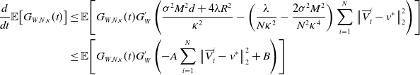 \begin{equation} \begin{aligned} \frac{d}{dt}\mathbb{E}\!\left [G_{W,N, \kappa }(t)\right ] &\leq \mathbb{E}\!\left [G_{W,N, \kappa }(t)G_W^{\prime }\left (\frac{\sigma ^2M^2d+ 4 \lambda R^2}{ \kappa ^2}-\left (\frac{ \lambda }{N\kappa ^2}-\frac{2\sigma ^2M^2}{N^2\kappa ^4}\right )\sum _{i=1}^N\big\| \overline{V}^i_t-v^* \big\|_2^2\right )\right ]\\ &\leq \mathbb{E}\!\left [G_{W,N, \kappa }(t)G_W^{\prime }\left ({-}{A}\sum _{i=1}^N\big\| \overline{V}^i_t-v^* \big\|_2^2+{B}\right )\right ] \end{aligned} \end{equation}
with $A\,:\!=\,\frac{\lambda }{N \kappa ^2}-\frac{2\sigma ^2M^2}{N^2 \kappa ^4}$
and
$A\,:\!=\,\frac{\lambda }{N \kappa ^2}-\frac{2\sigma ^2M^2}{N^2 \kappa ^4}$
and $B\,:\!=\,\frac{\sigma ^2M^2d+4\lambda R^2}{ \kappa ^2}$
. Now, if
$B\,:\!=\,\frac{\sigma ^2M^2d+4\lambda R^2}{ \kappa ^2}$
. Now, if $\sum _{i=1}^N\big\| \overline{V}^i_t-v^* \big\|_2^2\geq ({B-1})/{A}$
, we have
$\sum _{i=1}^N\big\| \overline{V}^i_t-v^* \big\|_2^2\geq ({B-1})/{A}$
, we have
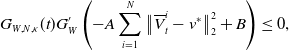 \begin{align*} G_{W,N, \kappa }(t)G_W^{\prime }\left ({-}{A}\sum _{i=1}^N\big\| \overline{V}^i_t-v^* \big\|_2^2+{B}\right )\leq 0, \end{align*}
while, if $\sum _{i=1}^N\big\| \overline{V}^i_t-v^* \big\|_2^2\leq ({B-1})/{A}$
, we have
$\sum _{i=1}^N\big\| \overline{V}^i_t-v^* \big\|_2^2\leq ({B-1})/{A}$
, we have
 \begin{align*} G_{W,N, \kappa }(t)G_W^{\prime }\left ({-}{A}\sum _{i=1}^N\big\| \overline{V}^i_t-v^* \big\|_2^2+{B}\right )\leq Be^{\frac{B-1}{N \kappa ^2A}}. \end{align*}
Thus, the latter inequality always holds true and consequently we have with (33)
 \begin{equation*} \begin{aligned} \frac{d}{dt}\mathbb{E}\!\left [G_{W,N, \kappa }(t)\right ]\leq Be^{\frac{B-1}{N \kappa ^2A}}, \end{aligned} \end{equation*}
which gives after integration
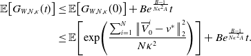 \begin{equation*} \begin{aligned} \mathbb{E}\!\left [G_{W,N, \kappa }(t)\right ] &\leq \mathbb{E}\!\left [G_{W,N, \kappa }(0)\right ]+Be^{\frac{B-1}{N \kappa ^2A}}t\\ &\leq \mathbb{E}\!\left [\exp \!\left (\frac{\sum _{i=1}^N\big\| \overline{V}^i_0-v^* \big\|_2^2}{N \kappa ^2}\right )\right ]+Be^{\frac{B-1}{N \kappa ^2A}}t. \end{aligned} \end{equation*}
Letting $W\to \infty$
, we eventually obtain
$W\to \infty$
, we eventually obtain
 \begin{equation} \mathbb{E}\!\left [\exp \!\left (\frac{\sum _{i=1}^N\big\| \overline{V}^i_t-v^* \big\|_2^2}{N \kappa ^2}\right )\right ] \leq \mathbb{E}\!\left [\exp \!\left (\frac{\sum _{i=1}^N\big\| \overline{V}^i_0-v^* \big\|_2^2}{N \kappa ^2}\right )\right ]+Be^{\frac{B-1}{N \kappa ^2A}}t\lt \infty, \end{equation}
provided that $\mathbb{E}\!\left [\exp \!\left({\sum _{i=1}^N\big\| \overline{V}^i_0-v^* \big\|_2^2}/{N \kappa ^2}\right)\right ]\lt \infty$
.
$\mathbb{E}\!\left [\exp \!\left({\sum _{i=1}^N\big\| \overline{V}^i_0-v^* \big\|_2^2}/{N \kappa ^2}\right)\right ]\lt \infty$
.
If $N\geq{(4 \sigma ^2 M^2)}/{(\lambda \kappa ^2)}$
, we have
$N\geq{(4 \sigma ^2 M^2)}/{(\lambda \kappa ^2)}$
, we have
 \begin{equation*} \frac {B-1}{N \kappa ^2A}\leq \frac {B}{N \kappa ^2A}=\frac {N\big(\sigma ^2M^2d+4\lambda R^2\big)}{\lambda N \kappa ^2-2\sigma ^2M^2}\leq C( \kappa,\lambda,\sigma,M,R,d). \end{equation*}
Thus, $C_{ \kappa }$
is upper-bounded and independent of
$C_{ \kappa }$
is upper-bounded and independent of $N$
.
$N$
.
Remark 9. The sub-Gaussianity of $\overline{V}_t$
follows from Lemma 8 by noticing that the statement can be applied in the setting
$\overline{V}_t$
follows from Lemma 8 by noticing that the statement can be applied in the setting $N=1$
when choosing
$N=1$
when choosing $\kappa$
sufficiently large.
$\kappa$
sufficiently large.
Remark 10. In Lemma 8, as the number of particles $N$
increases, the condition for
$N$
increases, the condition for $ \kappa$
to ensure
$ \kappa$
to ensure $C_{ \kappa }\lt \infty$
becomes more relaxed. Specifically, the value of
$C_{ \kappa }\lt \infty$
becomes more relaxed. Specifically, the value of $ \kappa$
can be as small as one needs as
$ \kappa$
can be as small as one needs as $N$
increases. This phenomenon can be easily understood by considering the limit as
$N$
increases. This phenomenon can be easily understood by considering the limit as $N$
approaches infinity. In this case,
$N$
approaches infinity. In this case, $C_{ \kappa }$
tends to
$C_{ \kappa }$
tends to $\sup _{t\in [0,T^*]}\exp \!\left(\mathbb{E}\!\left [\big\| \overline{V}_t-v^* \big\|_2^2\right ]/ \kappa ^2\right)$
. Therefore, as one shows an upper bound on the second moment of
$\sup _{t\in [0,T^*]}\exp \!\left(\mathbb{E}\!\left [\big\| \overline{V}_t-v^* \big\|_2^2\right ]/ \kappa ^2\right)$
. Therefore, as one shows an upper bound on the second moment of $\overline{V}_t$
, it becomes evident that
$\overline{V}_t$
, it becomes evident that $C_{ \kappa }$
remains finite as
$C_{ \kappa }$
remains finite as $N$
tends to infinity.
$N$
tends to infinity.
With the help of Lemma 8, we can now prove the following lemma.
Lemma 11. Let ${f} \in{\mathcal{C}}(\mathbb{R}^d)$
satisfy A1 and A3. Then, for any
${f} \in{\mathcal{C}}(\mathbb{R}^d)$
satisfy A1 and A3. Then, for any $t\in [0,T^*]$
,
$t\in [0,T^*]$
, $M$
and
$M$
and $R$
with
$R$
with $R\geq \left \| v_b-v^* \right \|_2$
finite, and
$R\geq \left \| v_b-v^* \right \|_2$
finite, and $N$
satisfying
$N$
satisfying $N\geq (16\alpha L_{\gamma }\sigma ^2M^2)/\lambda$
, we have
$N\geq (16\alpha L_{\gamma }\sigma ^2M^2)/\lambda$
, we have
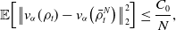 \begin{equation} \mathbb{E}\!\left [\left \| v_{\alpha }(\rho _t)-{v}_{\alpha }\!\left(\bar{\rho }_t^{ N}\right) \right \|_2^2\right ]\leq \frac{C_0}{N}, \end{equation}
where $C_0\,:\!=\,C_0(\lambda,\sigma,d,\alpha,L_{\gamma },L_u,T^*,R,v_b,v^*,M)$
.
$C_0\,:\!=\,C_0(\lambda,\sigma,d,\alpha,L_{\gamma },L_u,T^*,R,v_b,v^*,M)$
.
Proof. Without the loss of generality, we assume $v^*=0$
and recall that we assumed
$v^*=0$
and recall that we assumed $\underline{f}=0$
in the proofs as of Remark 6. We have
$\underline{f}=0$
in the proofs as of Remark 6. We have
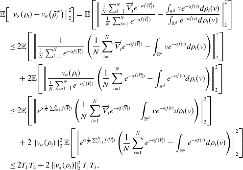 \begin{equation} \begin{aligned} &\mathbb{E}\!\left [\left \| v_{\alpha }(\rho _t)-{v}_{\alpha }\!\left(\bar{\rho }_t^{ N}\right) \right \|_2^2\right ]=\mathbb{E}\!\left [\left \| \frac{\frac{1}{N}\sum _{i=1}^N\overline{V}_t^ie^{-\alpha f(\mkern 1.5mu\overline{\mkern -1.5muV\mkern -1.5mu}\mkern 0mu_t^i)}}{\frac{1}{N}\sum _{i=1}^Ne^{-\alpha f(\mkern 1.5mu\overline{\mkern -1.5muV\mkern -1.5mu}\mkern 0mu_t^i)}}-\frac{\int _{\mathbb{R}^d}v e^{-\alpha f(v)}d\rho _t(v)}{\int _{\mathbb{R}^d}e^{-\alpha f(v)}d\rho _t(v)} \right \|_2^2\right ]\\ &\quad \leq 2\mathbb{E}\!\left [\left \| \frac{1}{\frac{1}{N}\sum _{i=1}^Ne^{-\alpha f(\mkern 1.5mu\overline{\mkern -1.5muV\mkern -1.5mu}\mkern 0mu_t^i)}}\left ({\frac{1}{N}\sum _{i=1}^N\overline{V}_t^ie^{-\alpha f(\mkern 1.5mu\overline{\mkern -1.5muV\mkern -1.5mu}\mkern 0mu_t^i)}}-{\int _{\mathbb{R}^d}v e^{-\alpha f(v)}d\rho _t(v)}\right ) \right \|_2^2\right ]\\ & \quad \quad \,+2\mathbb{E}\!\left [\left \| \frac{v_{\alpha }(\rho _t)}{\frac{1}{N}\sum _{i=1}^Ne^{-\alpha f(\mkern 1.5mu\overline{\mkern -1.5muV\mkern -1.5mu}\mkern 0mu_t^i)}}\left (\frac{1}{N}\sum _{i=1}^Ne^{-\alpha f(\mkern 1.5mu\overline{\mkern -1.5muV\mkern -1.5mu}\mkern 0mu_t^i)}-\int _{\mathbb{R}^d}e^{-\alpha f(v)}d\rho _t(v)\right ) \right \|_2^{2}\right ]\\ &\quad \leq 2\mathbb{E}\!\left [\left \| e^{\alpha \frac{1}{N}\sum _{i=1}^Nf(\mkern 1.5mu\overline{\mkern -1.5muV\mkern -1.5mu}\mkern 0mu_t^i)}\left ({\frac{1}{N}\sum _{i=1}^N\overline{V}_t^ie^{-\alpha f(\mkern 1.5mu\overline{\mkern -1.5muV\mkern -1.5mu}\mkern 0mu_t^i)}}-{\int _{\mathbb{R}^d}v e^{-\alpha f(v)}d\rho _t(v)}\right ) \right \|_2^2\right ]\\ &\quad \quad \,+2\left \| v_{\alpha }(\rho _t) \right \|_2^2\mathbb{E}\!\left [\left \| e^{\alpha \frac{1}{N}\sum _{i=1}^Nf(\mkern 1.5mu\overline{\mkern -1.5muV\mkern -1.5mu}\mkern 0mu_t^i)}\left (\frac{1}{N}\sum _{i=1}^Ne^{-\alpha f(\mkern 1.5mu\overline{\mkern -1.5muV\mkern -1.5mu}\mkern 0mu_t^i)}-\int _{\mathbb{R}^d}e^{-\alpha f(v)}d\rho _t(v)\right ) \right \|_2^{2}\right ]\\ &\quad \leq 2T_1 T_2+2\left \| v_{\alpha }(\rho _t) \right \|_2^2T_1 T_3, \end{aligned} \end{equation}
where we defined
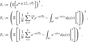 \begin{align*} T_1&\,:\!=\,\left (\mathbb{E}\!\left [{e^{4\alpha \frac{1}{N}\sum _{i=1}^Nf(\mkern 1.5mu\overline{\mkern -1.5muV\mkern -1.5mu}\mkern 0mu_t^i)}}\right ]\right )^{\frac{1}{2}},\\ T_2&\,:\!=\,\left (\mathbb{E}\!\left [\left \|{\frac{1}{N}\sum _{i=1}^N\overline{V}_t^ie^{-\alpha f(\mkern 1.5mu\overline{\mkern -1.5muV\mkern -1.5mu}\mkern 0mu_t^i)}}-{\int _{\mathbb{R}^d}v e^{-\alpha f(v)}d\rho _t(v)} \right \|_2^4\right ]\right )^{\frac{1}{2}},\\ T_3&\,:\!=\,\left (\mathbb{E}\!\left [\left \|{\frac{1}{N}\sum _{i=1}^Ne^{-\alpha f(\mkern 1.5mu\overline{\mkern -1.5muV\mkern -1.5mu}\mkern 0mu_t^i)}}-{\int _{\mathbb{R}^d}e^{-\alpha f(v)}d\rho _t(v)} \right \|_2^4\right ]\right )^{\frac{1}{2}}. \end{align*}
In the following, we upper-bound the terms $T_1, T_2$
and
$T_1, T_2$
and $ T_3$
separately. First, recall that by Lemma 8 we have for
$ T_3$
separately. First, recall that by Lemma 8 we have for $t\in [0,T^*]$
that
$t\in [0,T^*]$
that
 \begin{equation} \mathbb{E}\!\left [\exp \!\left (\frac{\sum _{i=1}^N\big\| \overline{V}_t^i \big\|_2^2}{N \kappa ^2}\right )\right ]\leq C_{ \kappa }\lt \infty, \end{equation}
where $C_{ \kappa }$
only depends on
$C_{ \kappa }$
only depends on $ \kappa,\lambda,\sigma,d,R,M$
and
$ \kappa,\lambda,\sigma,d,R,M$
and $T^*$
. With this,
$T^*$
. With this,
 \begin{equation*} \begin{aligned} T_1^2 = \mathbb{E}\!\left [{\exp \!\left ({4\alpha \frac{1}{N}\sum _{i=1}^Nf\big(\overline{V}_t^i\big)}\right )}\right ]&\leq \mathbb{E}\!\left [\exp \!\left (4\alpha \frac{1}{N}\sum _{i=1}^NL_{\gamma }\!\left (1+\big\| \overline{V}_t^i \big\|_2^{1+\gamma }\right )\right )\right ]\\ &\leq e^{4\alpha L_{\gamma }}\mathbb{E}\!\left [\exp \!\left (4\alpha L_{\gamma }\frac{1}{N}\sum _{i=1}^N\big\| \overline{V}_t^i \big\|_2^{1+\gamma }\right )\right ]\\ &\leq e^{8\alpha L_{\gamma }}\mathbb{E}\!\left [\exp\! \left (4\alpha L_{\gamma }\frac{1}{N}\sum _{i=1}^N\big\| \overline{V}_t^i \big\|_2^{2}\right )\right ]\\ &=e^{8\alpha L_{\gamma }}\mathbb{E}\!\left [\exp\! \left (\frac{1}{ \kappa ^2}\frac{1}{N}\sum _{i=1}^N\big\| \overline{V}_t^i \big\|_2^{2}\right )\right ] \\ &\leq e^{8\alpha L_{\gamma }}C_{ \kappa }\!\!\mid _{ \kappa =\frac{1}{2\sqrt{\alpha L_{\gamma }}}}, \end{aligned} \end{equation*}
where we set $ \kappa ^2={1}/{(4\alpha L_{\gamma })}$
in the next-to-last step and where
$ \kappa ^2={1}/{(4\alpha L_{\gamma })}$
in the next-to-last step and where $N$
should satisfy
$N$
should satisfy $N\geq (16\alpha L_{\gamma }\sigma ^2M^2)/\lambda$
.
$N\geq (16\alpha L_{\gamma }\sigma ^2M^2)/\lambda$
.
Second, we have
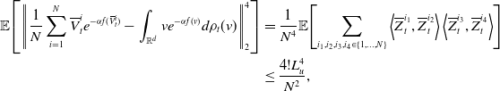 \begin{equation*} \begin{aligned} \mathbb{E}\!\left [\left \|{\frac{1}{N}\sum _{i=1}^N\overline{V}_t^ie^{-\alpha f(\mkern 1.5mu\overline{\mkern -1.5muV\mkern -1.5mu}\mkern 0mu_t^i)}}-{\int _{\mathbb{R}^d}v e^{-\alpha f(v)}d\rho _t(v)} \right \|_2^4\right ]&=\frac{1}{N^4}\mathbb{E}\!\left [\sum _{i_1,i_2,i_3,i_4\in \{1,\dots,N\}}\left \lt \overline{Z}_t^{i_1}, \overline{Z}_t^{i_2} \right \gt \left \lt \overline{Z}_t^{i_3}, \overline{Z}_t^{i_4} \right \gt \right ]\\ &\leq \frac{4!L_u^4}{N^2}, \end{aligned} \end{equation*}
where $\left (\overline{Z}_t^i\,:\!=\,\overline{V}_t^ie^{-\alpha f(\mkern 1.5mu\overline{\mkern -1.5muV\mkern -1.5mu}\mkern 0mu_t^i)}-{\int _{\mathbb{R}^d}v e^{-\alpha f(v)}d\rho _t(v)}\right )_{i=1,\dots,N}$
are i.i.d. and have zero mean. Thus,
$\left (\overline{Z}_t^i\,:\!=\,\overline{V}_t^ie^{-\alpha f(\mkern 1.5mu\overline{\mkern -1.5muV\mkern -1.5mu}\mkern 0mu_t^i)}-{\int _{\mathbb{R}^d}v e^{-\alpha f(v)}d\rho _t(v)}\right )_{i=1,\dots,N}$
are i.i.d. and have zero mean. Thus,
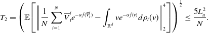 \begin{equation*} T_2 = \left (\mathbb {E}\!\left [\left \| {\frac {1}{N}\sum _{i=1}^N\overline {V}_t^ie^{-\alpha f(\mkern 1.5mu\overline {\mkern -1.5muV\mkern -1.5mu}\mkern 0mu_t^i)}}-{\int _{\mathbb {R}^d}v e^{-\alpha f(v)}d\rho _t(v)} \right \|_2^4\right ]\right )^{\frac {1}{2}}\leq \frac {5L_u^2}{N}. \end{equation*}
Similarly, we can derive
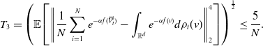 \begin{equation*} T_3 = \left (\mathbb {E}\!\left [\left \| {\frac {1}{N}\sum _{i=1}^Ne^{-\alpha f(\mkern 1.5mu\overline {\mkern -1.5muV\mkern -1.5mu}\mkern 0mu_t^i)}}-{\int _{\mathbb {R}^d}e^{-\alpha f(v)}d\rho _t(v)} \right \|_2^4\right ]\right )^{\frac {1}{2}}\leq \frac {5}{N}. \end{equation*}
Collecting the bounds for the terms $T_1$
,
$T_1$
, $T_2$
and
$T_2$
and $T_3$
and inserting them in (36), we obtain
$T_3$
and inserting them in (36), we obtain
 \begin{equation} \begin{aligned} \mathbb{E}\!\left [\left \| v_{\alpha }(\rho _t)-{v}_{\alpha }(\bar{\rho }_t) \right \|_2^2\right ]&\leq 10e^{6\alpha L_{\gamma }}C_{ \kappa }^{\frac{1}{2}}\!\!\mid _{ \kappa =\frac{1}{2\sqrt{\alpha L_{\gamma }}}}\left (L_u^2+\sup _{t\in [0,T^*]}\left \| v_{\alpha }(\rho _t) \right \|_2^2\right )\frac{1}{N}. \end{aligned} \end{equation}
Since by Lemmas 14, 16 and 17, we know that $\left \| v_{\alpha }(\rho _t) \right \|_2$
can be uniformly bounded by a constant depending on
$\left \| v_{\alpha }(\rho _t) \right \|_2$
can be uniformly bounded by a constant depending on $\alpha,\lambda,\sigma,d,R,v_b,v^*,M,L_{\nu }$
and
$\alpha,\lambda,\sigma,d,R,v_b,v^*,M,L_{\nu }$
and $\nu$
(see in particular Equation (48) that combines the aforementioned lemmas), we can conclude (38) with
$\nu$
(see in particular Equation (48) that combines the aforementioned lemmas), we can conclude (38) with
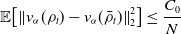 \begin{equation} \mathbb{E}\!\left [\left \| v_{\alpha }(\rho _t)-{v}_{\alpha }(\bar{\rho }_t) \right \|_2^2\right ]\leq \frac{C_0}{N} \end{equation}
for some constant $C_0$
depends on
$C_0$
depends on $\lambda,\sigma,d,\alpha,L_{\nu },\nu,L_{\gamma },L_u,T^*,R,v_b,v^*$
and
$\lambda,\sigma,d,\alpha,L_{\nu },\nu,L_{\gamma },L_u,T^*,R,v_b,v^*$
and $M$
.
$M$
.
3.2.2. Upper bound for the third term in (19)
In this section, we bound Term $III$
of the error decomposition (19). Before stating the main result of this section, Proposition 15, we first need to provide two auxiliary lemmas, Lemma 12 and Lemma 14.
$III$
of the error decomposition (19). Before stating the main result of this section, Proposition 15, we first need to provide two auxiliary lemmas, Lemma 12 and Lemma 14.
Lemma 12. Let $R,M\in (0,\infty )$
. Then, it holds
$R,M\in (0,\infty )$
. Then, it holds
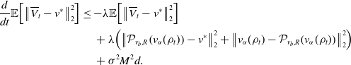 \begin{equation} \begin{aligned} \frac{d}{dt}\mathbb{E}\!\left [ \big\| \overline{V}_t-v^* \big\|_2^2\right ] &\leq -\lambda \mathbb{E}\!\left [ \big\| \overline{V}_t-v^* \big\|_2^2\right ]\\ &\quad \,+\lambda \!\left (\left \| \mathcal{P}_{v_b,R}\!\left (v_{\alpha }(\rho _t)\right )-v^* \right \|_2^2+\left \| v_{\alpha }(\rho _t)-\mathcal{P}_{v_b,R}\!\left (v_{\alpha }(\rho _t)\right ) \right \|_2^2\right )\\ &\quad \,+\sigma ^2M^2d. \end{aligned} \end{equation}
If further $\lambda \geq 2\sigma ^2d$
, we have
$\lambda \geq 2\sigma ^2d$
, we have
 \begin{equation} \begin{aligned} \frac{d}{dt}\mathbb{E}\!\left [ \big\| \overline{V}_t-v^* \big\|_2^2\right ] &\leq -\lambda \mathbb{E}\!\left [ \big\| \overline{V}_t-v^* \big\|_2^2\right ]\\ &\quad \,+\lambda \!\left (\left \| \mathcal{P}_{v_b,R}\!\left (v_{\alpha }(\rho _t)\right )-v^* \right \|_2^2+\left \| v_{\alpha }(\rho _t)-\mathcal{P}_{v_b,R}\!\left (v_{\alpha }(\rho _t)\right ) \right \|_2^2\right ). \end{aligned} \end{equation}
Proof. By Itô’s formula, we have
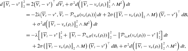 \begin{equation*} \begin{aligned} d \big\| \overline{V}_t-v^* \big\|_2^2&=2\!\left (\overline{V}_t-v^*\right )^{\top }d \overline{V}_t+\sigma ^2 d\!\left (\left \| \overline{V}_t-v_{\alpha }(\rho _t) \right \|_2^2\wedge M^2\right )dt\\ &=-2\lambda \!\left \lt \overline{V}_t-v^*, \overline{V}_t-\mathcal{P}_{v_b,R}\!\left (v_{\alpha }(\rho _t)\right ) \right \gt dt+2\sigma \!\left (\left \| \overline{V}_t-v_{\alpha }(\rho _t) \right \|_2\wedge M\right )\left (\overline{V}_t-v^*\right )^{\top }dB_t\\ &\quad \,+\sigma ^2 d\!\left (\left \| \overline{V}_t-v_{\alpha }(\rho _t) \right \|_2^2\wedge M^2\right )dt\\ &=-\lambda \!\left [\big\| \overline{V}_t-v^* \big\|_2^2+\left \| \overline{V}_t-\mathcal{P}_{v_b,R}\!\left (v_{\alpha }(\rho _t)\right ) \right \|_2^2-\left \| \mathcal{P}_{v_b,R}\!\left (v_{\alpha }(\rho _t)\right )-v^* \right \|_2^2\right ]dt\\ &\quad \,+2\sigma \!\left (\left \| \overline{V}_t-v_{\alpha }(\rho _t) \right \|_2\wedge M\right )\left (\overline{V}_t-v^*\right )^{\top }dB_t+\sigma ^2 d\!\left (\left \| \overline{V}_t-v_{\alpha }(\rho _t) \right \|_2^2\wedge M^2\right )dt, \end{aligned} \end{equation*}
which, after taking the expectation on both sides, yields
 \begin{equation} \begin{aligned} \frac{d}{dt}\mathbb{E}\!\left [ \big\| \overline{V}_t-v^* \big\|_2^2\right ]&= -\lambda \mathbb{E}\!\left [ \big\| \overline{V}_t-v^* \big\|_2^2\right ]\\&\quad \,+\lambda \!\left \| \mathcal{P}_{v_b,R}\!\left (v_{\alpha }(\rho _t)\right )-v^* \right \|_2^2-\lambda \mathbb{E}\!\left [\left \| \overline{V}_t-\mathcal{P}_{v_b,R}\!\left (v_{\alpha }(\rho _t)\right ) \right \|_2^2\right ]\\ &\quad \,+\sigma ^2 d\mathbb{E}\!\left [\left \| \overline{V}_t-v_{\alpha }(\rho _t) \right \|_2^2\wedge M^2\right ]. \end{aligned} \end{equation}
For the term $\mathbb{E}\!\left [\left \| \overline{V}_t-\mathcal{P}_{v_b,R}\!\left (v_{\alpha }(\rho _t)\right ) \right \|_2^2\right ]$
, we notice that
$\mathbb{E}\!\left [\left \| \overline{V}_t-\mathcal{P}_{v_b,R}\!\left (v_{\alpha }(\rho _t)\right ) \right \|_2^2\right ]$
, we notice that
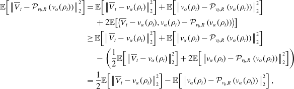 \begin{equation*} \begin {aligned} \mathbb {E}\!\left [\left \| \overline {V}_t-\mathcal {P}_{v_b,R}\left (v_{\alpha }(\rho _t)\right ) \right \|_2^2\right ]&=\mathbb {E}\!\left [ \left \| \overline {V}_t-v_{\alpha }(\rho _t) \right \|_2^2\right ]+\mathbb {E}\!\left [\left \| v_{\alpha }(\rho _t)-\mathcal {P}_{v_b,R}\left (v_{\alpha }(\rho _t)\right ) \right \|_2^2\right ]\\ &\quad \,+2\mathbb {E}\!\left [\left \lt \overline {V}_t-v_{\alpha }(\rho _t), v_{\alpha }(\rho _t)-\mathcal {P}_{v_b,R}\left (v_{\alpha }(\rho _t)\right ) \right \gt \right ]\\ &\geq \mathbb {E}\!\left [ \left \| \overline {V}_t-v_{\alpha }(\rho _t) \right \|_2^2\right ]+\mathbb {E}\!\left [\left \| v_{\alpha }(\rho _t)-\mathcal {P}_{v_b,R}\left (v_{\alpha }(\rho _t)\right ) \right \|_2^2\right ]\\ &\quad \,-\left (\frac {1}{2}\mathbb {E}\!\left [\left \| \overline {V}_t-v_{\alpha }(\rho _t) \right \|_2^2\right ]+2\mathbb {E}\!\left [\left \| v_{\alpha }(\rho _t)-\mathcal {P}_{v_b,R}\left (v_{\alpha }(\rho _t)\right ) \right \|_2^2\right ]\right )\\ &=\frac {1}{2}\mathbb {E}\!\left [\left \| \overline {V}_t-v_{\alpha }(\rho _t) \right \|_2^2\right ]-\mathbb {E}\!\left [\left \| v_{\alpha }(\rho _t)-\mathcal {P}_{v_b,R}\left (v_{\alpha }(\rho _t)\right ) \right \|_2^2\right ], \end {aligned} \end{equation*}
which, inserted into Equation (42), allows to derive
 \begin{equation*} \begin {aligned} \frac {d}{dt}\mathbb {E}\!\left [ \left \| \overline {V}_t-v^* \right \|_2^2\right ]&\leq -\lambda \mathbb {E}\!\left [ \left \| \overline {V}_t-v^* \right \|_2^2\right ]\\&\quad \,+\lambda \left (\left \| \mathcal {P}_{v_b,R}\left (v_{\alpha }(\rho _t)\right )-v^* \right \|_2^2+\left \| v_{\alpha }(\rho _t)-\mathcal {P}_{v_b,R}\left (v_{\alpha }(\rho _t)\right ) \right \|_2^2\right )\\ &\quad \,-\frac {1}{2}\lambda \mathbb {E}\!\left [\left \| \overline {V}_t-v_{\alpha }(\rho _t) \right \|_2^2\right ]+\sigma ^2 d\left (\left \| \overline {V}_t-v_{\alpha }(\rho _t) \right \|_2^2\wedge M^2\right ). \end {aligned} \end{equation*}
From this, we get for any $\lambda$
and
$\lambda$
and $\sigma$
that
$\sigma$
that
 \begin{equation} \begin{aligned} \frac{d}{dt}\mathbb{E}\!\left [ \big\| \overline{V}_t-v^* \big\|_2^2\right ]&\leq -\lambda \mathbb{E}\!\left [ \big\| \overline{V}_t-v^* \big\|_2^2\right ]\\&\quad \,+\lambda \left (\left \| \mathcal{P}_{v_b,R}\!\left (v_{\alpha }(\rho _t)\right )-v^* \right \|_2^2+\left \| v_{\alpha }(\rho _t)-\mathcal{P}_{v_b,R}\!\left (v_{\alpha }(\rho _t)\right ) \right \|_2^2\right )\\ &\quad \,+\sigma ^2M^2d \end{aligned} \end{equation}
as well as
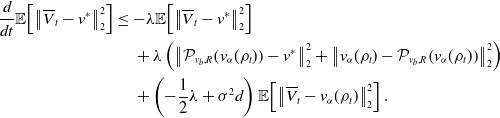 \begin{equation} \begin{aligned} \frac{d}{dt}\mathbb{E}\!\left [ \big\| \overline{V}_t-v^* \big\|_2^2\right ] &\leq -\lambda \mathbb{E}\!\left [ \big\| \overline{V}_t-v^* \big\|_2^2\right ]\\&\quad \,+\lambda \left (\left \| \mathcal{P}_{v_b,R}\!\left (v_{\alpha }(\rho _t)\right )-v^* \right \|_2^2+\left \| v_{\alpha }(\rho _t)-\mathcal{P}_{v_b,R}\!\left (v_{\alpha }(\rho _t)\right ) \right \|_2^2\right )\\ &\quad \,+\left ({-}\frac{1}{2}\lambda +\sigma ^2d\right )\mathbb{E}\!\left [\left \| \overline{V}_t-v_{\alpha }(\rho _t) \right \|_2^2\right ]. \end{aligned} \end{equation}
If $\lambda \geq 2\sigma ^2d$
, by Equation (44), we get
$\lambda \geq 2\sigma ^2d$
, by Equation (44), we get
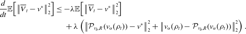 \begin{equation} \begin{aligned} \frac{d}{dt}\mathbb{E}\!\left [ \big\| \overline{V}_t-v^* \big\|_2^2\right ]&\leq -\lambda \mathbb{E}\!\left [ \big\| \overline{V}_t-v^* \big\|_2^2\right ]\\&\quad \,+\lambda \left (\left \| \mathcal{P}_{v_b,R}\!\left (v_{\alpha }(\rho _t)\right )-v^* \right \|_2^2+\left \| v_{\alpha }(\rho _t)-\mathcal{P}_{v_b,R}\!\left (v_{\alpha }(\rho _t)\right ) \right \|_2^2\right ). \end{aligned} \end{equation}
Remark 13. When $R=M=\infty$
, we can show
$R=M=\infty$
, we can show
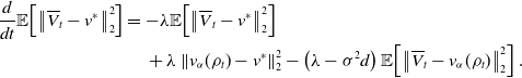 \begin{equation*} \begin {aligned}\frac {d}{dt}\mathbb {E}\!\left [\left \| {\overline {V}}_t-v^* \right \|_2^2\right ]&= -\lambda \mathbb {E}\!\left [\left \| {\overline {V}}_t-v^* \right \|_2^2\right ]\\&\quad \,+\lambda \left \| v_{\alpha }(\rho _t)-v^* \right \|_2^2-\left (\lambda -\sigma ^2d\right )\mathbb {E}\!\left [\left \| \overline {V}_t-v_{\alpha }(\rho _t) \right \|_2^2\right ]. \end {aligned} \end{equation*}
If further $\lambda \geq \sigma ^2d$
, we have
$\lambda \geq \sigma ^2d$
, we have
 \begin{equation*}\frac {d}{dt}\mathbb {E}\!\left [\left \| {\overline {V}}_t-v^* \right \|_2^2\right ]\leq -\lambda \mathbb {E}\!\left [\left \| {\overline {V}}_t-v^* \right \|_2^2\right ]+\lambda \left \| v_{\alpha }(\rho _t)-v^* \right \|_2^2. \end{equation*}
This differs from [Reference Fornasier, Klock and Riedl10, Lemma 18].
The next result is a quantitative version of the Laplace principle as established in [Reference Fornasier, Klock and Riedl10, Proposition 21].
Lemma 14. For any $r\gt 0$
, define
$r\gt 0$
, define $f_r\,:\!=\, \sup _{v \in B_r\left (v^*\right )} f(v)$
. Then, under the inverse continuity condition A2, for any
$f_r\,:\!=\, \sup _{v \in B_r\left (v^*\right )} f(v)$
. Then, under the inverse continuity condition A2, for any $r \in \left (0, R_0\right ]$
and
$r \in \left (0, R_0\right ]$
and $q\gt 0$
such that
$q\gt 0$
such that $q+f_r \leq f_{\infty }$
, it holds
$q+f_r \leq f_{\infty }$
, it holds
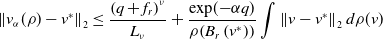 \begin{equation} \left \|v_\alpha (\rho )-v^*\right \|_2 \leq \frac{\left (q+f_r\right )^\nu }{L_{\nu }}+\frac{\exp \!({-}\alpha q)}{\rho\! \left (B_r\left (v^*\right )\right )} \int \left \| v-v^* \right \|_2 d \rho (v) \end{equation}
With the above preparation, we can now upper bound Term $III$
. We have by Jensen’s inequality
$III$
. We have by Jensen’s inequality
 \begin{equation} III=\mathbb{E}\!\left [\left \| \frac{1}{N} \sum _{i=1}^N \overline{V}_{T^*}^i-v^* \right \|_2^2\right ]\leq \frac{1}{N}\sum _{i=1}^N\mathbb{E}\!\left [\left \| \overline{V}_{T^*}^i-v^* \right \|_2^2\right ], \end{equation}
that is, it is enough to upper-bound $\mathbb{E}\!\left [\left \| \overline{V}_{T^*}-v^* \right \|_2^2\right ]$
, which is the content of the next statement.
$\mathbb{E}\!\left [\left \| \overline{V}_{T^*}-v^* \right \|_2^2\right ]$
, which is the content of the next statement.
Proposition 15. Let ${f} \in{\mathcal{C}}(\mathbb{R}^d)$
satisfy A1, A2 and A3. Moreover, let
${f} \in{\mathcal{C}}(\mathbb{R}^d)$
satisfy A1, A2 and A3. Moreover, let $\rho _0\in{\mathcal{P}}_4(\mathbb{R}^d)$
with
$\rho _0\in{\mathcal{P}}_4(\mathbb{R}^d)$
with $v^*\in \operatorname{supp}(\rho _0)$
. Fix any
$v^*\in \operatorname{supp}(\rho _0)$
. Fix any $\epsilon \in (0,W_2^2(\rho _0,\delta _{v^*}))$
and define the time horizon
$\epsilon \in (0,W_2^2(\rho _0,\delta _{v^*}))$
and define the time horizon
 \begin{equation*}T^*\,:\!=\,\frac {1}{\lambda }\log \left (\frac {2W_2^2(\rho _0,\delta _{v^*})}{\epsilon }\right ).\end{equation*}
Moreover, let $R\in (\!\left \| v_b-v^* \right \|_2+\sqrt{\epsilon/2},\infty )$
,
$R\in (\!\left \| v_b-v^* \right \|_2+\sqrt{\epsilon/2},\infty )$
, $M\in (0,\infty )$
and
$M\in (0,\infty )$
and $\lambda,\sigma \gt 0$
be such that
$\lambda,\sigma \gt 0$
be such that $\lambda \geq 2\sigma ^2d$
or
$\lambda \geq 2\sigma ^2d$
or $\sigma ^2M^2d=\mathcal{O}(\epsilon )$
. Then, we can choose
$\sigma ^2M^2d=\mathcal{O}(\epsilon )$
. Then, we can choose $\alpha$
sufficiently large, depending on
$\alpha$
sufficiently large, depending on $\lambda,\sigma,d,T^*,R,v_b,M,\epsilon$
and properties of
$\lambda,\sigma,d,T^*,R,v_b,M,\epsilon$
and properties of $f$
, such that
$f$
, such that $ \mathbb{E}\!\left [\left \| \overline{V}_{T^*}-v^* \right \|_2^2\right ] =\mathcal{O}(\epsilon )$
.
$ \mathbb{E}\!\left [\left \| \overline{V}_{T^*}-v^* \right \|_2^2\right ] =\mathcal{O}(\epsilon )$
.
Proof. We only prove the case $\lambda \geq 2\sigma ^2d$
in detail. The case
$\lambda \geq 2\sigma ^2d$
in detail. The case $\sigma ^2M^2d=\mathcal{O}(\epsilon )$
follows similarly.
$\sigma ^2M^2d=\mathcal{O}(\epsilon )$
follows similarly.
According to Lemmas 14 and 17, we have
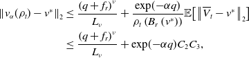 \begin{equation} \begin{aligned} \left \|v_{\alpha }(\rho _t)-v^*\right \|_2 &\leq \frac{\left (q+f_r\right )^\nu }{L_{\nu }}+\frac{\exp \!({-}\alpha q)}{\rho _t\left (B_r\left (v^*\right )\right )} \mathbb{E}\!\left [\big\| \overline{V}_t-v^* \big\|_2\right ] \\ &\leq \frac{\left (q+f_r\right )^\nu }{L_{\nu }}+{\exp \!({-}\alpha q)}C_{2}C_{3}, \end{aligned} \end{equation}
where $C_{2}\,:\!=\,(\!\exp{q^{\prime}T^*})/{C_{4}}\lt \infty$
,
$C_{2}\,:\!=\,(\!\exp{q^{\prime}T^*})/{C_{4}}\lt \infty$
, $q^{\prime}$
and
$q^{\prime}$
and $C_4$
are from Lemma 17, and where, as of Lemma 16,
$C_4$
are from Lemma 17, and where, as of Lemma 16, $C_{3}\,:\!=\,\sup _{[0,T^*]}\mathbb{E}\!\left [\big\| \overline{V}_t-v^* \big\|_2\right ]\lt \infty$
. In what follows, let us deal with the two terms on the right-hand side of (48). For the term
$C_{3}\,:\!=\,\sup _{[0,T^*]}\mathbb{E}\!\left [\big\| \overline{V}_t-v^* \big\|_2\right ]\lt \infty$
. In what follows, let us deal with the two terms on the right-hand side of (48). For the term ${\left (q+f_r\right )^\nu }/{L_{\nu }}$
, let
${\left (q+f_r\right )^\nu }/{L_{\nu }}$
, let $q=f_r$
. Then by A2 and A3, we can choose proper
$q=f_r$
. Then by A2 and A3, we can choose proper $r$
, such that
$r$
, such that $2(L_{\nu } r)^{{1}/{\nu }}\leq 2f_r\leq f_{\infty }$
. Further by A3, we have
$2(L_{\nu } r)^{{1}/{\nu }}\leq 2f_r\leq f_{\infty }$
. Further by A3, we have
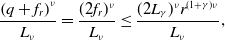 \begin{equation*} \frac {\left (q+f_r\right )^\nu }{L_{\nu }}=\frac {(2f_r)^{\nu }}{L_{\nu }}\leq \frac {(2L_{\gamma })^{\nu }r^{(1+\gamma )\nu }}{L_{\nu }}, \end{equation*}
so if
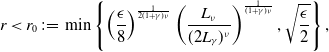 \begin{equation*} r\lt r_0\,:\!=\,\min \left \{\left (\frac {\epsilon }{8}\right )^{\frac {1}{2(1+\gamma )\nu }}\left (\frac {L_{\nu }}{(2L_{\gamma })^{\nu }}\right )^{\frac {1}{(1+\gamma )\nu }},\sqrt {\frac {\epsilon }{2}}\right \}, \end{equation*}
we can bound
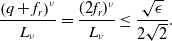 \begin{equation*} \frac {\left (q+f_r\right )^\nu }{L_{\nu }}=\frac {(2f_r)^{\nu }}{L_{\nu }}\leq \frac {\sqrt {\epsilon }}{2\sqrt {2}}. \end{equation*}
For term ${\exp \!({-}\alpha q)}C_{2}C_{3}$
, we can choose
${\exp \!({-}\alpha q)}C_{2}C_{3}$
, we can choose $\alpha$
large enough such that
$\alpha$
large enough such that
 \begin{equation*} {\exp \!({-}\alpha q)}C_{2}C_{3}\leq \frac {\sqrt {\epsilon }}{2\sqrt {2}}. \end{equation*}
With these choices of $r$
and
$r$
and $\alpha$
and by integrating them into Equation (48), we obtain
$\alpha$
and by integrating them into Equation (48), we obtain
 \begin{equation*}\left \| v_{\alpha }(\rho _t)-v^* \right \|_2^2\lt \frac {\epsilon }{2}, \end{equation*}
for all $t\in [0,T^*]$
, and thus
$t\in [0,T^*]$
, and thus
 \begin{equation*} \left \| v_{\alpha }(\rho _t)-v_b \right \|_2\leq \left \| v_{\alpha }(\rho _t)-v^* \right \|_2+\left \| v^*-v_b \right \|_2\leq \sqrt {\frac {\epsilon }{2}}+\left \| v^*-v_b \right \|_2\leq R. \end{equation*}
Consequently, by Lemma 12, we have
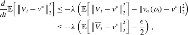 \begin{equation*}\begin {aligned} \frac {d}{dt}\mathbb {E}\!\left [ \left \| \overline {V}_t-v^* \right \|_2^2\right ]&\leq -\lambda \left (\mathbb {E}\!\left [\left \| \overline {V}_t-v^* \right \|_2^2\right ]-\left \| v_{\alpha }(\rho _t)-v^* \right \|_2^2\right )\\&\leq -\lambda \left (\mathbb {E}\!\left [\left \| \overline {V}_t-v^* \right \|_2^2\right ]-\frac {\epsilon }{2}\right ), \end {aligned} \end{equation*}
since now $\mathcal{P}_{v_b,R}(v_{\alpha }(\rho _t))=v_{\alpha }(\rho _t)$
. Finally by Grönwall’s inequality,
$\mathcal{P}_{v_b,R}(v_{\alpha }(\rho _t))=v_{\alpha }(\rho _t)$
. Finally by Grönwall’s inequality, $\mathbb{E}\!\left [\left \| \overline{V}_{T^*}-v^* \right \|_2^2\right ]\leq \epsilon$
.
$\mathbb{E}\!\left [\left \| \overline{V}_{T^*}-v^* \right \|_2^2\right ]\leq \epsilon$
.
Lemma 16. Let $\left \| v_b-v^* \right \|_2\lt R\lt \infty$
and
$\left \| v_b-v^* \right \|_2\lt R\lt \infty$
and $0\lt M\lt \infty$
. Then, it holds
$0\lt M\lt \infty$
. Then, it holds
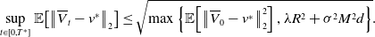 \begin{equation} \sup _{t\in [0,T^*]}\mathbb{E}\!\left [\big\| \overline{V}_t-v^* \big\|_2\right ]\leq \sqrt{\max \left \{\mathbb{E}\!\left [ \left \| \overline{V}_0-v^* \right \|_2^2\right ],\lambda R^2+\sigma ^2M^2d\right \}}. \end{equation}
Proof. By Equation (42), we have
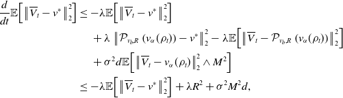 \begin{equation*} \begin {aligned} \frac {d}{dt}\mathbb {E}\!\left [ \left \| \overline {V}_t-v^* \right \|_2^2\right ]&\leq -\lambda \mathbb {E}\!\left [ \left \| \overline {V}_t-v^* \right \|_2^2\right ]\\&\quad \,+\lambda \left \| \mathcal {P}_{v_b,R}\left (v_{\alpha }(\rho _t)\right )-v^* \right \|_2^2-\lambda \mathbb {E}\!\left [\left \| \overline {V}_t-\mathcal {P}_{v_b,R}\left (v_{\alpha }(\rho _t)\right ) \right \|_2^2\right ]\\ &\quad \,+\sigma ^2 d\mathbb {E}\!\left [\left \| \overline {V}_t-v_{\alpha }(\rho _t) \right \|_2^2\wedge M^2\right ]\\ &\leq -\lambda \mathbb {E}\!\left [ \left \| \overline {V}_t-v^* \right \|_2^2\right ]+\lambda R^2+\sigma ^2M^2d, \end {aligned} \end{equation*}
yielding
 \begin{equation*} \mathbb {E}\!\left [ \left \| \overline {V}_t-v^* \right \|_2^2\right ]\leq \max \left \{\mathbb {E}\!\left [ \left \| \overline {V}_0-v^* \right \|_2^2\right ],\lambda R^2+\sigma ^2M^2d\right \}, \end{equation*}
after an application of Grönwall’s inequality for any $t\geq 0$
.
$t\geq 0$
.
Lemma 17. For any $M\in (0,\infty )$
,
$M\in (0,\infty )$
, $\tau \geq 1$
,
$\tau \geq 1$
, $r\gt 0$
and
$r\gt 0$
and $R\in (\!\left \| v_b-v^* \right \|_2+r,\infty )$
, it holds
$R\in (\!\left \| v_b-v^* \right \|_2+r,\infty )$
, it holds
 \begin{equation*} \begin {aligned} \rho _t\left (B_r\left (v^*\right )\right ) & \geq C_4\exp \!({-}q^{\prime} t)\gt 0, \end {aligned} \end{equation*}
where
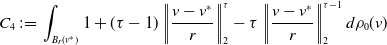 \begin{align*} C_4\,:\!=\,\int _{B_r(v^*)}1+(\tau -1)\left \| \frac{v-v^*}{r} \right \|_2^{\tau }-\tau \left \| \frac{v-v^*}{r} \right \|_2^{\tau -1} d \rho _0(v) \end{align*}
and where $q^{\prime}$
depends on
$q^{\prime}$
depends on $\tau,\lambda,\sigma,d,r,R,v_b$
and
$\tau,\lambda,\sigma,d,r,R,v_b$
and $M$
.
$M$
.
Proof. Recall that the law $\rho _t$
of
$\rho _t$
of $\overline{V}_t$
satisfies the Fokker–Planck equation
$\overline{V}_t$
satisfies the Fokker–Planck equation
 \begin{equation*} \partial _t \rho _t=\lambda \operatorname {div}\left (\left (v-\mathcal {P}_{v_b,R}\left (v_{\alpha }(\rho _t)\right )\right )\rho _t\right )+\frac {\sigma ^2}{2} \Delta \left (\left (\left \|v-v_\alpha \left (\rho _t\right )\right \|^2\wedge M^2\right ) \rho _t\right ). \end{equation*}
Let us first define for $\tau \geq 1$
the test function
$\tau \geq 1$
the test function
 \begin{equation} \phi _r^{\tau }(v)\,:\!=\,\begin{cases} 1+(\tau -1)\left \| \frac{v}{r} \right \|_2^{\tau }-\tau \left \| \frac{v}{r} \right \|_2^{\tau -1},& \left \| v \right \|_2\leq r,\\ 0,& \text{else}, \end{cases} \end{equation}
for which it is easy to verify that $\phi _r^{\tau }\in \mathcal{C}_c^1(\mathbb{R}^d,[0,1])$
. Since
$\phi _r^{\tau }\in \mathcal{C}_c^1(\mathbb{R}^d,[0,1])$
. Since $\textrm{Im}\,\phi _r^{\tau }\subset [0,1]$
, we have
$\textrm{Im}\,\phi _r^{\tau }\subset [0,1]$
, we have $\rho _t(B_r(v^*))\geq \int _{B_r(v^*)}\phi _r^{\tau }(v-v^*)\,d\rho _t(v)$
. To lower bound
$\rho _t(B_r(v^*))\geq \int _{B_r(v^*)}\phi _r^{\tau }(v-v^*)\,d\rho _t(v)$
. To lower bound $\rho _t(B_r(v^*))$
, it is thus sufficient to establish a lower bound on
$\rho _t(B_r(v^*))$
, it is thus sufficient to establish a lower bound on $\int _{B_r(v^*)}\phi _r^{\tau }(v-v^*)\,d\rho _t(v)$
. By Green’s formula,
$\int _{B_r(v^*)}\phi _r^{\tau }(v-v^*)\,d\rho _t(v)$
. By Green’s formula,
 \begin{equation*} \begin {aligned} &\frac {d}{dt}\int _{B_r(v^*)}\phi _r^{\tau }(v-v^*)\,d\rho _t(v)=-\lambda \int _{B_r(v^*)}\left \lt v-\mathcal {P}_{v_b,R}\left (v_{\alpha }(\rho _t)\right ), \nabla \phi _r^{\tau }(v-v^*) \right \gt d\rho _t(v)\\ &\quad \,\quad +\frac {\sigma ^2}{2}\int _{B_r(v^*)}\left (\left \| v-v_{\alpha }(\rho _t) \right \|_2^2\wedge M^2\right )\Delta \phi _r^{\tau }(v-v^*)d\rho _t(v)\\ &\quad \,=\tau (\tau -1)\int _{B_r(v^*)}\frac {\left \| v-v^* \right \|_2^{\tau -3}}{r^{\tau -3}}\Bigg (\!\left (1-\frac {\left \| v-v^* \right \|_2}{r}\right )\bigg (\lambda \left \lt \frac {v-\mathcal {P}_{v_b,R}\left (v_{\alpha }(\rho _t)\right )}{r}, \frac {v-v^*}{r} \right \gt \\ &\quad \,\quad -\frac {\sigma ^2}{2}\left (d+\tau -2\right )\frac {\left \| v-v_{\alpha }(\rho _t) \right \|_2^2\wedge M^2}{r^2}\bigg )+\frac {\sigma ^2}{2}\frac {\left \| v-v_{\alpha }(\rho _t) \right \|_2^2\wedge M^2}{r^2}\Bigg )d\rho _t(v). \end {aligned} \end{equation*}
For simplicity, let us abbreviate
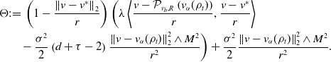 \begin{equation*} \begin {aligned} \Theta &:\!=\,\left (1-\frac {\left \| v-v^* \right \|_2}{r}\right )\bigg (\lambda \left \lt \frac {v-\mathcal {P}_{v_b,R}\left (v_{\alpha }(\rho _t)\right )}{r}, \frac {v-v^*}{r} \right \gt \\ &\quad -\frac {\sigma ^2}{2}\left (d+\tau -2\right )\frac {\left \| v-v_{\alpha }(\rho _t) \right \|_2^2\wedge M^2}{r^2}\bigg ) +\frac {\sigma ^2}{2}\frac {\left \| v-v_{\alpha }(\rho _t) \right \|_2^2\wedge M^2}{r^2}. \end {aligned} \end{equation*}
We can choose $\epsilon _1$
small enough, depending on
$\epsilon _1$
small enough, depending on $\tau$
and
$\tau$
and $d$
, such that when
$d$
, such that when ${\left \| v-v^* \right \|_2}/{r}\gt 1-\epsilon _1$
, we have
${\left \| v-v^* \right \|_2}/{r}\gt 1-\epsilon _1$
, we have
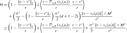 \begin{equation*} \begin {aligned} \Theta & =\left (1-\frac {\left \| v-v^* \right \|_2}{r}\right )\lambda \left \lt \frac {v-\mathcal {P}_{v_b,R}\left (v_{\alpha }(\rho _t)\right )}{r}, \frac {v-v^*}{r} \right \gt \\ & \quad \,+\bigg (\frac {\sigma ^2}{2}-\left (1-\frac {\left \| v-v^* \right \|_2}{r}\right )\frac {\sigma ^2}{2}(d+\tau -2)\bigg )\frac {\left \| v-v_{\alpha }(\rho _t) \right \|_2^2\wedge M^2}{r^2}\\ &\geq \left (1-\frac {\left \| v-v^* \right \|_2}{r}\right )\lambda \left \lt \frac {v-\mathcal {P}_{v_b,R}\left (v_{\alpha }(\rho _t)\right )}{r}, \frac {v-v^*}{r} \right \gt +\frac {\sigma ^2}{3}\frac {\left \| v-v_{\alpha }(\rho _t) \right \|_2^2\wedge M^2}{r^2}, \end {aligned} \end{equation*}
where the last inequality works if ${\left \| v-v^* \right \|_2}/{r}\geq 1-1/(6(d+\tau -2))$
.
${\left \| v-v^* \right \|_2}/{r}\geq 1-1/(6(d+\tau -2))$
.
If $v_{\alpha }(\rho _t)\not \in B_{R}(v_b)$
, we have
$v_{\alpha }(\rho _t)\not \in B_{R}(v_b)$
, we have $\left |{\left \lt v-\mathcal{P}_{v_b,R}\!\left (v_{\alpha }(\rho _t)\right ), v-v^* \right \gt }\right |/r^2\leq C(r,R,v_b)$
and, since
$\left |{\left \lt v-\mathcal{P}_{v_b,R}\!\left (v_{\alpha }(\rho _t)\right ), v-v^* \right \gt }\right |/r^2\leq C(r,R,v_b)$
and, since $R\gt \left \| v_b-v^* \right \|_2+r$
,
$R\gt \left \| v_b-v^* \right \|_2+r$
, $({\left \| v-v_{\alpha }(\rho _t) \right \|_2^2\wedge M^2})/{r^2}\geq C(r,M,R,v_b)$
, which allows to choose
$({\left \| v-v_{\alpha }(\rho _t) \right \|_2^2\wedge M^2})/{r^2}\geq C(r,M,R,v_b)$
, which allows to choose $\epsilon _2$
small enough, depending on
$\epsilon _2$
small enough, depending on $\lambda,r,\sigma,R,v_b$
and
$\lambda,r,\sigma,R,v_b$
and $M$
, such that
$M$
, such that $\Theta \gt 0$
when
$\Theta \gt 0$
when ${\left \| v-v^* \right \|_2}/{r}\gt 1-\min \{\epsilon _1,\epsilon _2\}$
.
${\left \| v-v^* \right \|_2}/{r}\gt 1-\min \{\epsilon _1,\epsilon _2\}$
.
If $v_{\alpha }(\rho _t)\in B_{R}(v_b)$
and
$v_{\alpha }(\rho _t)\in B_{R}(v_b)$
and $\left \| v-v_{\alpha }(\rho _t) \right \|_2\leq M$
, we have by Lemma 18
$\left \| v-v_{\alpha }(\rho _t) \right \|_2\leq M$
, we have by Lemma 18
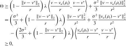 \begin{equation*} \begin {aligned} \Theta &\geq \left (1-\frac {\left \| v-v^* \right \|_2}{r}\right )\lambda \left \lt \frac {v-v_{\alpha }(\rho _t)}{r}, \frac {v-v^*}{r} \right \gt +\frac {\sigma ^2}{3}\frac {\left \| v-v_{\alpha }(\rho _t) \right \|_2^2}{r^2}\\ &=\left (\frac {\sigma ^2}{3}+\left (1-\frac {\left \| v-v^* \right \|_2}{r}\right )\lambda \right )\frac {\left \| v-v^* \right \|_2^2}{r^2}+\frac {\sigma ^2}{3}\frac {\left \| v_{\alpha }(\rho _t)-v^* \right \|_2^2}{r^2}\\ &\quad \,-\left (\frac {2\sigma ^2}{3}+\left (1-\frac {\left \| v-v^* \right \|_2}{r}\right )\lambda \right )\left \lt \frac {v_{\alpha }(\rho _t)-v^*}{r}, \frac {v-v^*}{r} \right \gt \\ &\geq 0, \end {aligned} \end{equation*}
when $\left \| v-v^* \right \|_2/r\in \left [1-2\sigma ^2/(3\lambda ),1\right ]$
.
$\left \| v-v^* \right \|_2/r\in \left [1-2\sigma ^2/(3\lambda ),1\right ]$
.
If $v_{\alpha }(\rho _t)\in B_{R}(v_b)$
and
$v_{\alpha }(\rho _t)\in B_{R}(v_b)$
and $\left \| v-v_{\alpha }(\rho _t) \right \|_2\gt M$
, we have
$\left \| v-v_{\alpha }(\rho _t) \right \|_2\gt M$
, we have
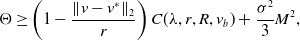 \begin{equation*} \Theta \geq \left (1-\frac {\left \| v-v^* \right \|_2}{r}\right )C(\lambda,r,R,v_b)+\frac {\sigma ^2}{3}M^2, \end{equation*}
that is, we can choose $\epsilon _3$
small enough, depending on
$\epsilon _3$
small enough, depending on $\lambda,r,\sigma,R,v_b$
and
$\lambda,r,\sigma,R,v_b$
and $M$
, such that
$M$
, such that $\Theta \geq 0$
when
$\Theta \geq 0$
when ${\left \| v-v^* \right \|_2}/{r}\gt 1-\min \{\epsilon _1,\epsilon _2,\epsilon _3,{2\sigma ^2}/{3\lambda }\}$
.
${\left \| v-v^* \right \|_2}/{r}\gt 1-\min \{\epsilon _1,\epsilon _2,\epsilon _3,{2\sigma ^2}/{3\lambda }\}$
.
Combining the cases from above, we conclude that $\Theta \geq 0$
when
$\Theta \geq 0$
when ${\left \| v-v^* \right \|_2}/{r}\geq 1-\min \{\epsilon _1,\epsilon _2,\epsilon _3,{2\sigma ^2}/{3\lambda }\}$
. On the other hand, when
${\left \| v-v^* \right \|_2}/{r}\geq 1-\min \{\epsilon _1,\epsilon _2,\epsilon _3,{2\sigma ^2}/{3\lambda }\}$
. On the other hand, when ${\left \| v-v^* \right \|_2}/{r}\leq 1-\min \{\epsilon _1,\epsilon _2,\epsilon _3,{2\sigma ^2}/{3\lambda }\}$
, we have
${\left \| v-v^* \right \|_2}/{r}\leq 1-\min \{\epsilon _1,\epsilon _2,\epsilon _3,{2\sigma ^2}/{3\lambda }\}$
, we have
 \begin{equation*} \begin {aligned} \tau (\tau -1)\frac {\left \| v-v^* \right \|_2^{\tau -3}}{r^{\tau -3}}\Theta &=\tau (\tau -1)\frac {\left \| v-v^* \right \|_2^{\tau -3}}{r^{\tau -3}}\frac {\Theta }{\phi _r^{\tau }(v)}\phi _r^{\tau }(v-v^*)\geq -C_5\phi _r^{\tau }(v-v^*) \end {aligned} \end{equation*}
for some constant $C_5$
depending on
$C_5$
depending on $r,R,M,v_b,\lambda,\sigma,d$
and
$r,R,M,v_b,\lambda,\sigma,d$
and $\tau$
, since
$\tau$
, since $\left |{\Theta }\right |$
is upper-bounded and
$\left |{\Theta }\right |$
is upper-bounded and $\phi _r^{\tau }(v-v^*)\geq \phi _r^{\tau }((1-\min \{\epsilon _1,\epsilon _2,\epsilon _3,{2\sigma ^2}/{3\lambda }\})r)\gt 0$
for any
$\phi _r^{\tau }(v-v^*)\geq \phi _r^{\tau }((1-\min \{\epsilon _1,\epsilon _2,\epsilon _3,{2\sigma ^2}/{3\lambda }\})r)\gt 0$
for any $v$
satisfies
$v$
satisfies ${\left \| v-v^* \right \|_2}/{r}\leq 1-\min \{\epsilon _1,\epsilon _2,\epsilon _3,{2\sigma ^2}/{3\lambda }\}$
.
${\left \| v-v^* \right \|_2}/{r}\leq 1-\min \{\epsilon _1,\epsilon _2,\epsilon _3,{2\sigma ^2}/{3\lambda }\}$
.
All in all we have
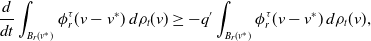 \begin{equation*} \begin {aligned} \frac {d}{dt}\int _{B_r(v^*)}\phi _r^{\tau }(v-v^*)\,d\rho _t(v)\geq -q^{\prime}\int _{B_r(v^*)} \phi _r^{\tau }(v-v^*)\,d\rho _t(v), \end {aligned} \end{equation*}
where $q^{\prime}\,:\!=\,\max \{C_5,0\}$
. By Grönwall’s inequality, we thus have
$q^{\prime}\,:\!=\,\max \{C_5,0\}$
. By Grönwall’s inequality, we thus have
 \begin{equation*} \rho _t(B_r(v^*))\geq \int _{B_r(v^*)}\phi _r^{\tau }(v-v^*)\,d\rho _t(v)\geq e^{-q^{\prime}t}\int _{B_r(v^*)}\phi _r^{\tau }(v-v^*)\,d\rho _0(v), \end{equation*}
which concludes the proof.
Lemma 18. Let $a,b\gt 0$
. Then, we have
$a,b\gt 0$
. Then, we have
 \begin{equation*} (a+b(1-x))x^2+ay^2-(2a+b(1-x))xy\geq 0, \end{equation*}
for any $x\in [1-{2a}/{b},1]\cap (0,\infty )$
and
$x\in [1-{2a}/{b},1]\cap (0,\infty )$
and $y\geq 0$
.
$y\geq 0$
.
Proof. For $y=0$
, this is true. For
$y=0$
, this is true. For $y\gt 0$
, divide both side by
$y\gt 0$
, divide both side by $ay^2$
and denote
$ay^2$
and denote $c={b}/{a}$
. Then the lemma is equivalent to showing
$c={b}/{a}$
. Then the lemma is equivalent to showing $(1+c(1-x))\left (x/y\right )^2-(2+c(1-x))x/y+1\geq 0$
, that is, it is enough to show
$(1+c(1-x))\left (x/y\right )^2-(2+c(1-x))x/y+1\geq 0$
, that is, it is enough to show $\min _{r\geq 0}\!(1+c(1-x))r^2-(2+c(1-x))r+1\geq 0$
, when
$\min _{r\geq 0}\!(1+c(1-x))r^2-(2+c(1-x))r+1\geq 0$
, when $x\in [1-{2}/{c},1]$
. We have
$x\in [1-{2}/{c},1]$
. We have
 \begin{equation*} \arg \min _{r}\!(1+c(1-x))r^2-(2+c(1-x))r+1 = \frac {2+c(1-x)}{2+2c(1-x)}, \end{equation*}
and thus
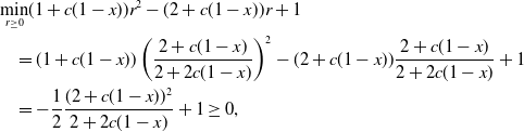 \begin{equation*} \begin {aligned} &\min _{r\geq 0}\!(1+c(1-x))r^2-(2+c(1-x))r+1\\ &\quad =(1+c(1-x))\left (\frac {2+c(1-x)}{2+2c(1-x)}\right )^2-(2+c(1-x))\frac {2+c(1-x)}{2+2c(1-x)}+1\\ &\quad =-\frac {1}{2}\frac {(2+c(1-x))^2}{2+2c(1-x)}+1\geq 0, \end {aligned} \end{equation*}
when $x\in [1-{2}/{c},1]$
. This finishes the proof.
$x\in [1-{2}/{c},1]$
. This finishes the proof.
4. Numerical experiments
In this section, we numerically demonstrate the benefit of using CBO with truncated noise. For isotropic [Reference Pinnau, Totzeck, Tse and Martin7, Reference Carrillo, Choi, Totzeck and Tse8, Reference Fornasier, Klock and Riedl10] and anisotropic noise [Reference Carrillo, Jin, Li and Zhu9, Reference Fornasier, Klock, Riedl, Laredo, Hidalgo and Babaagba11], we compare the CBO method with truncation $M=1$
to standard CBO for several benchmark problems in optimisation, which are summarised in Table 1.
$M=1$
to standard CBO for several benchmark problems in optimisation, which are summarised in Table 1.
Table 1. Benchmark test functions
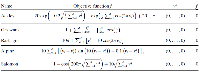
In the subsequent tables, we report comparison results for the two methods for the different benchmark functions as well as different numbers of particles $N$
and, potentially, different numbers of steps
$N$
and, potentially, different numbers of steps $K$
. Throughout, we set
$K$
. Throughout, we set $v_b=0$
and
$v_b=0$
and $R=\infty$
, which is out of convenience. Any sufficiently large but finite choice for
$R=\infty$
, which is out of convenience. Any sufficiently large but finite choice for $R$
yields identical results.
$R$
yields identical results.
The success criterion is defined by achieving the condition $\left \| \frac{1}{N}\sum _{i=1}^N V^i_{{K,\Delta t}}-v^* \right \|_2\leq 0.1$
, which ensures that the algorithm has reached the basin of attraction of the global minimiser. The success rate is averaged over
$\left \| \frac{1}{N}\sum _{i=1}^N V^i_{{K,\Delta t}}-v^* \right \|_2\leq 0.1$
, which ensures that the algorithm has reached the basin of attraction of the global minimiser. The success rate is averaged over $1000$
runs.
$1000$
runs.
4.1. Isotropic case
Let $d=15$
. In the case of isotropic noise, we always set
$d=15$
. In the case of isotropic noise, we always set $\lambda =1$
,
$\lambda =1$
, $\sigma =0.3$
,
$\sigma =0.3$
, $\alpha =10^5$
and step size
$\alpha =10^5$
and step size $\Delta t=0.02$
. The initial positions
$\Delta t=0.02$
. The initial positions $(V_0^i)_{i=1,\dots,N}$
are sampled i.i.d. from
$(V_0^i)_{i=1,\dots,N}$
are sampled i.i.d. from $\rho _0=\mathcal{N}(0,I_d)$
. In Table 2, we report results comparing the isotropic CBO method with truncation
$\rho _0=\mathcal{N}(0,I_d)$
. In Table 2, we report results comparing the isotropic CBO method with truncation $M=1$
and the original isotropic CBO method [Reference Pinnau, Totzeck, Tse and Martin7, Reference Carrillo, Choi, Totzeck and Tse8, Reference Fornasier, Klock and Riedl10] (
$M=1$
and the original isotropic CBO method [Reference Pinnau, Totzeck, Tse and Martin7, Reference Carrillo, Choi, Totzeck and Tse8, Reference Fornasier, Klock and Riedl10] ( $M=+\infty$
) for the Ackley, Griewank and Salomon function. Each algorithm is run for
$M=+\infty$
) for the Ackley, Griewank and Salomon function. Each algorithm is run for $K=200$
steps.
$K=200$
steps.
Table 2. For the $15$
-dimensional Ackley and Salomon function, the CBO method with truncation (
$15$
-dimensional Ackley and Salomon function, the CBO method with truncation ( $M=1$
) is able to locate the global minimum using only
$M=1$
) is able to locate the global minimum using only $N=300$
particles. In comparison, even with an larger number of particles (up to
$N=300$
particles. In comparison, even with an larger number of particles (up to $N=1200$
), the original CBO method (
$N=1200$
), the original CBO method ( $M=+\infty$
) cannot achieve a flawless success rate. In the case of the Griewank function, the original CBO method (
$M=+\infty$
) cannot achieve a flawless success rate. In the case of the Griewank function, the original CBO method ( $M=+\infty$
) exhibits a quite low success rate, even when utilising
$M=+\infty$
) exhibits a quite low success rate, even when utilising $N=1200$
particles. Contrarily, in the same setting, the CBO method with truncation (
$N=1200$
particles. Contrarily, in the same setting, the CBO method with truncation ( $M=1$
) achieves a success rate of
$M=1$
) achieves a success rate of $0.791.$
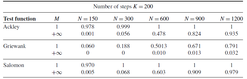
Since the benchmark functions Rastrigin and Alpine are more challenging, we use more particles $N$
and a larger number of steps
$N$
and a larger number of steps $K$
, namely
$K$
, namely $K=200$
and
$K=200$
and $K=500$
. We report the results in Table 3.
$K=500$
. We report the results in Table 3.
Table 3. For the $15$
-dimensional Rastrigin and Alpine function, both algorithms have difficulties in finding the global minimiser. However, the success rates for the CBO method with truncation (
$15$
-dimensional Rastrigin and Alpine function, both algorithms have difficulties in finding the global minimiser. However, the success rates for the CBO method with truncation ( $M=1$
) are significantly higher compared to those of the original CBO method (
$M=1$
) are significantly higher compared to those of the original CBO method ( $M=+\infty.$
)
$M=+\infty.$
)
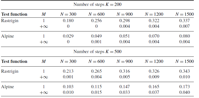
4.2. Anisotropic case
Let $d=20$
. In the case of anisotropic noise, we set
$d=20$
. In the case of anisotropic noise, we set $\lambda =1,\sigma =5,\alpha =10^5$
and step size
$\lambda =1,\sigma =5,\alpha =10^5$
and step size $\Delta t=0.02$
. The initial positions of the particles are initialised with
$\Delta t=0.02$
. The initial positions of the particles are initialised with $\rho _0=\mathcal{N}(0,100I_d)$
. In Table 4, we report results comparing the anisotropic CBO method with truncation
$\rho _0=\mathcal{N}(0,100I_d)$
. In Table 4, we report results comparing the anisotropic CBO method with truncation $M=1$
and the original anisotropic CBO method [Reference Carrillo, Jin, Li and Zhu9, Reference Fornasier, Klock, Riedl, Laredo, Hidalgo and Babaagba11] (
$M=1$
and the original anisotropic CBO method [Reference Carrillo, Jin, Li and Zhu9, Reference Fornasier, Klock, Riedl, Laredo, Hidalgo and Babaagba11] ( $M=+\infty$
) for the Rastrigin, Ackley, Griewank and Salomon function. Each algorithm is run for
$M=+\infty$
) for the Rastrigin, Ackley, Griewank and Salomon function. Each algorithm is run for $K=200$
steps.
$K=200$
steps.
Table 4. For the $20$
-dimensional Rastrigin, Ackley and Salomon function, the original anisotropic CBO method (
$20$
-dimensional Rastrigin, Ackley and Salomon function, the original anisotropic CBO method ( $M=+\infty$
) works better than the anisotropic CBO method with truncation (
$M=+\infty$
) works better than the anisotropic CBO method with truncation ( $M=1$
), in particular when the particle number
$M=1$
), in particular when the particle number $N$
is small. In the case of the Salomon function, when increasing the number of particle to
$N$
is small. In the case of the Salomon function, when increasing the number of particle to $N=900$
, the success rates of the original anisotropic CBO method (
$N=900$
, the success rates of the original anisotropic CBO method ( $M=+\infty$
) decreases. In the case of the Griewank function, however, we find that the anisotropic CBO method with truncation (
$M=+\infty$
) decreases. In the case of the Griewank function, however, we find that the anisotropic CBO method with truncation ( $M=+\infty$
) works considerably better than the original anisotropic CBO method (
$M=+\infty$
) works considerably better than the original anisotropic CBO method ( $M=1.$
)
$M=1.$
)
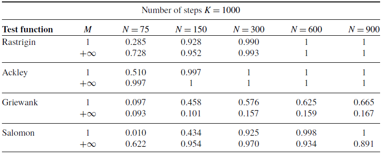
Since the benchmark function Alpine is more challenging and none of the algorithms work in the previous setting, we reduce the dimensionality to $d=15$
, choose
$d=15$
, choose $\sigma =1$
, use
$\sigma =1$
, use $\rho _0=\mathcal{N}(0,I_d)$
to initialise, employ more particles and use a larger number of steps
$\rho _0=\mathcal{N}(0,I_d)$
to initialise, employ more particles and use a larger number of steps $K$
, namely
$K$
, namely $K=200$
,
$K=200$
, $K=500$
and
$K=500$
and $K=1000$
. We report the results in Table 5.
$K=1000$
. We report the results in Table 5.
Table 5.
For the $15$
-dimensional Alpine function, the anisotropic CBO method with truncated noise (
$15$
-dimensional Alpine function, the anisotropic CBO method with truncated noise ( $M=1$
) works better than the original anisotropic CBO method (
$M=1$
) works better than the original anisotropic CBO method ( $M=+\infty.$
)
$M=+\infty.$
)
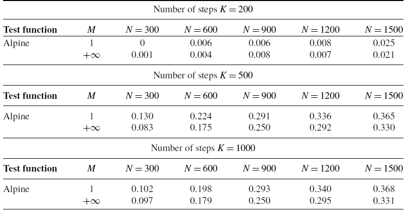
5. Conclusions
In this paper, we establish the convergence to a global minimiser of a potentially non-convex and non-smooth objective function for a variant of CBO which incorporates truncated noise. We observe that truncating the noise in CBO enhances the well-behavedness of the statistics of the law of the dynamics, which enables enhanced convergence performance and allows in particular for a wider flexibility in choosing the noise parameter of the method, as we observe numerically. For rigorously proving the convergence of the implementable algorithm to the global minimiser of the objective, we follow the route devised in [Reference Fornasier, Klock and Riedl10].
Acknowledgements
MF acknowledges the support of the Munich Center for Machine Learning. PR acknowledges the support of the Extreme Computing Research Center at KAUST. KR acknowledges the support of the Munich Center for Machine Learning and the financial support from the Technical University of Munich – Institute for Ethics in Artificial Intelligence (IEAI). LS acknowledges the support of KAUST Optimization and Machine Learning Lab. LS also thanks the hospitality of the Chair of Applied Numerical Analysis of the Technical University of Munich for discussions that contributed to the finalisation of this work.
Funding statement
This work has been funded by the KAUST Baseline Research Scheme and the German Federal Ministry of Education and Research, and the Bavarian State Ministry for Science and the Arts.
Competing interests
None.


 Open access