


I
In this article, we examine how pre-industrial markets functioned under multi-currency conditions and how market networks facilitated the spread of different currencies by looking at the nineteenth-century currency system in Finland. The evidence we present adds to the existing literature on multi-currency regimes by providing a greater level of detail about the function and economic importance of these systems.
By historical standards, single national currencies are novelties. Virtually every pre-industrial country had a monetary system characterised by multiple mediums of exchange, and often multiple units of account. For example, there were thousands of different bank notes circulating in the antebellum United States; in the 1760s some 2,000 shopkeepers in Mexico City were issuing their own tokens made of base metal (Jaremski Reference Jaremski2011; Helleiner Reference Helleiner2003, pp. 23-4); while in the Holy Roman Empire of the fifteenth century about 500 active mints produced at least 70 different currencies (Boerner and Volckart Reference Boerner and Volckart2011).
Currency conditions were complex to the point where it was commonplace to have foreign currencies circulating within a domestic market. According to Fernand Braudel (Reference Braudel1990, p. 601), a combination of foreign and domestic currencies was the norm before the nineteenth century – foreign coins, for example, were an important part of both Canadian and Latin American monetary systems (Greenfield & Rockoff Reference Greenfield and Rockoff1995; Helleiner Reference Helleiner2003, p. 21). As late as 1857, Mexican pesos and a number of other foreign coins were legal tender in the United States (Briones and Rockoff Reference Briones and Rockoff2005, p. 281). In this respect, it is not surprising that the American monetary union in the nineteenth century was designed to deliver a common unit of account and a standard of deferred payment, rather than a uniform medium of exchange (Michener and Wright Reference Michener and Wright2006, p. 20).
Driven by – among other things – a lack of strict state control, an absence of central bank monopolies in issuing legal tender, insufficient supply of reliable domestic currency, and the slow diffusion of information, multi-currency systems prevailed for a long time – and they continue to do so in the modern developing world (e.g. Burdett et al. Reference Burdett, Trejos and Wright2001, p. 120; Li Reference Li2002, p. 436; Craig and Waller Reference Craig and Waller2000, p. 2; Reference Craig and Waller2004; Helleiner Reference Helleiner2003; Engdahl and Ögren Reference Engdahl and Ögren2008, p. 89; Volckart Reference Volckart2017, pp. 9-12). Simultaneously, these systems pose fundamental questions for the economic actors involved: how will businesses, workers and organisations pick the currency in which to post their prices, ask for their wages, or hold their transaction balances (Greenfield and Rockoff Reference Greenfield and Rockoff1996, p. 903; Goldberg and Tille Reference Goldberg and Tille2008)? Multi-currency conditions also give rise to macro-economic effects such as loss of seigniorage (due to foreign currencies being in circulation), and restrictions on monetary policy freedom. A multi-currency system not only limits a central bank's capacity to print money the public is willing to hold, but also its ability to act as the guarantor and lender of last resort (Capannelli and Menon Reference Capannelli and Menon2010).
The more complex the currency conditions are, the more pressing the various negative externalities ought to become. However, the harmfulness of a multi-currency system depends heavily on an important, yet generally unconfirmed assumption that economic actors were using all (or a sufficient share) of the currencies in circulation. Unfortunately, however, relatively little is known about how widely various currencies were used, and who was using them. Where appropriate statistics are available, the previous literature has revealed that money supplies consisted of coins and notes in various currencies (e.g. Friedman and Schwartz Reference Friedman and Schwartz1963, pp. 322-3; Briones and Rockoff Reference Briones and Rockoff2005, pp. 285, 293; Engdahl and Ögren Reference Engdahl and Ögren2008; Edvinsson Reference Edvinsson2012; Svensson Reference Svensson2017, pp. 189-92). This corresponds to the observed plurality of exchange rate notations (e.g. Boerner and Volckart Reference Boerner and Volckart2011; Jaremski Reference Jaremski2011; Flandreau et al. Reference Flandreau, Galimard, Jobst and Nogués-Marco2009). Unfortunately, both of these findings provide only circumstantial evidence concerning the actual use of different currencies.
Due to this lack of concrete quantitative evidence, the assertion that multi-currency environments were complicated often rests on narrative sources. Kuroda (Reference Kuroda2008), for instance, draws attention to nineteenth-century concerns over the ‘chaotic’ currency conditions that supposedly existed in China. Rather than taking these at face value, he argues that the monetary system of the Far East might well have worked more effectively than would have been immediately apparent to an outsider. Similarly, Briones and Rockoff (Reference Briones and Rockoff2005) argue that modern observers tend to dismiss multi-currency systems as confusing or poorly functioning due to a lack of contextual knowledge – many commentators have little, if any, first-hand experience of currency plurality.
To gain a better understanding of multi-currency systems and their economic implications, this article focuses on Finnish currency conditions during the first half of the nineteenth century. In 1809, having been part of the Swedish Realm for some 700 years, Finland was annexed to Russia. As an autonomous part of the Russian Empire Finland kept its Swedish legislation and institutions, and this lingering Swedish influence also took a monetary form: until the 1840s there was a mixture of half a dozen forms of exchange in circulation, of both Swedish and Russian origin.
Using novel parish-level data, we contribute to existing literature by showing that currencies were positively spatially autocorrelated – in other words, clusters of neighbouring regions used the same currency. This implies that the multi-currency system mainly existed as an aggregate. We ran straightforward regression models to show that a substantial amount of the spatial variation in the rural distribution of currencies can be explained by the trade connections between rural regions and towns as well as between rural parishes themselves.
This article has six sections: the following section reviews existing literature on the various strategies that have been taken to adapt to a multi-currency regime; the third section presents the data used for our purposes here; the fourth and fifth sections present an analysis of the Finnish currency system and link its spatial features to market networks; while the sixth section offers some conclusions.
II
Following the influential work of Mundell (Reference Mundell1961), it has been assumed that adopting a single currency between trading partners reduces the transaction costs in the exchange of goods and services (Frankel and Rose Reference Frankel and Rose1998, p. 1009; Alesina and Barro Reference Alesina and Barro2001). Concurringly, Helleiner (Reference Helleiner2003) has suggested that the emergence of integrated within-country markets was a result of regional currencies being eradicated, and Boerner and Volckart (Reference Boerner and Volckart2011) argue that the monetary fragmentation of Germany from the fourteenth to mid sixteenth century was a result of weak market integration and that sheer political will was not enough to integrate markets under fragmented monetary conditions.
Given the prevalence and scope of multi-currency systems, it seems only reasonable to ask how transactions were made in such a complicated monetary environment. The classic argument, often associated with Friedrich A. Hayek, stresses the importance of free markets (Hayek Reference Hayek1976; Greenfield and Rockoff Reference Greenfield and Rockoff1996; Briones and Rockoff Reference Briones and Rockoff2005, pp. 280-1). Hayek envisioned a ‘denationalized’ monetary system, where private actors would issue competing currencies. Private competition would solve the problem of over-supply and a currency that was depreciating would be abandoned in favour of another that was not. Craig and Waller (Reference Craig and Waller2004) have theorised in Hayekian fashion that if economic actors use two different currencies – one risky and one safe – and the riskiness of the other currency increases, the safe currency progressively replaces it as a medium of exchange. In this way, the economy should eventually tip towards a single-currency equilibrium.
Free market theories such as these are not totally divorced from reality. According to Matt Jaremski's analysis of free banking in the US, the discount on different bank notes was determined by markets in which note holders monitored risky behaviour. They were able to do so in spite of significant travel costs, informational asymmetries and minimal government involvement. In their analysis of private banking era notes in Michigan, Christopher Bailey et al. (Reference Bailey, Hossain and Pecquet2018) concur with Jaremski's analysis, but say that when many currencies or currency substitutes were simultaneously in use for an extended period, the role of exchange brokers in everyday business increased. As an interesting take on the evolution of transaction costs, they consider the emergence of such brokers as costs for a financial system that used both heterogeneous currencies and money substitutes.
The easiest ‘bank-free’ route towards a single-currency equilibrium is to minimise the risk related to exchange rates by keeping transactions requiring price negotiation to a minimum. The most likely way to achieve this is if sellers post prices in the most prominent currency (Greenfield & Rockoff Reference Greenfield and Rockoff1995, p. 1092; Selgin Reference Selgin1996, pp. 638-40).
Engdahl and Ögren (Reference Engdahl and Ögren2008) point out an important contextual reason why nationwide single currency systems did not emerge in the pre-modern era: the money supply of any single currency might have been too small to allow for homogenisation of the national currency environment. This is only true, however, if all the currencies were used widely enough (i.e. on a national scale), and there is compelling evidence to prove that they were not. Currencies have been shown to follow stratified circulation patterns determined by, for instance, various social or regional factors. For example, the dual monetary system of the Bengal Sultanate (1205–1576) was distinctly layered: silver coins were used to meet the needs of government and trade, while cyprai moneta shells were used for the low-value transactions made by most of the rest of the population (Deyell Reference Deyell2010). Particularly revealing is Kuroda's (Reference Kuroda2008) account of imperial and early republican China, where different money was used for different commodities even within the same city. In the 1910s, in Jiujiang – a treaty port in Jiangxi province – there were several silver dollars simultaneously in circulation, but each with its own circuit. The Mexican dollar, for instance, was used exclusively for tea and porcelain, since these goods were exported via Shanghai, where the currency was prominent.
Meanwhile, Boerner and Volckart (Reference Boerner and Volckart2011, p. 54) have shown the geographically distinct use of silver and gold currencies in medieval Europe; Sweden had, until the mid thirteenth century, three different areas with their own coinage (Svensson Reference Svensson2017); and thousands of unauthorised coins were issued by London businesses that often circulated no further afield than several city blocks (Helleiner Reference Helleiner2003, pp. 23-4). Regional currencies were also widely used in nineteenth-century Italy and Japan (Helleiner Reference Helleiner2003, pp. 64-5, Greenfield and Rockoff Reference Greenfield and Rockoff1995).
One particularly well-documented case of regional circulation is that of the Californian gold standard after the 1860s. At this point, the US had a monetary system which in theory used both gold and paper money, but the national legal tender (the greenback dollar) never gained a foothold in California. A similar situation occurred when the gold standard was retained in Northern Ireland after the Bank Restriction Act of 1797 (Greenfield & Rockoff Reference Greenfield and Rockoff1995, pp. 1095, 1097; Selgin Reference Selgin1996, p. 640).
We think that the analysis of this kind of stratified circulation deserves more attention. Whilst we are aware that it will by no means provide a panacea, an understanding of the geographical patterns of currency distribution will greatly enhance our knowledge about the real economic impact of these systems. The following sections thus analyse the evidence from nineteenth-century Finland as a good example of regionally stratified circulation.
III
Not only does previous research on multi-currency systems play an important part in understanding Finnish monetary history in the early 1800s, but the Finnish experience also offers insights into this previous research.
We focus on the period from 1809 up until the 1840s. We pick 1809 as the start date, as this was when, after some 700 years under the Swedish rule, Finland was annexed to Russia, and the silver rouble became the official currency and legal tender of the country.
The silver rouble had been the legal tender of the Russian Empire since 1704, but paper money (the so-called assignation rouble) that started being issued in 1769 was already replacing the silver rouble in the late eighteenth century. In 1812, Tsar Alexander I declared assignation roubles the national currency of the Empire, while the silver rouble retained its position as a unit of account (Denzel Reference Denzel2010, pp. 359-60; Kuusterä and Tarkka Reference Kuusterä and Tarkka2011, pp. 73, 79-82).
In spite of its official position, it took some 30 years for the rouble to replace the Swedish currency in daily transactions. This happened in the 1840s when a uniform silver-pegged rouble was introduced across the whole Russian Empire. For the first three decades of Russian rule, Finland's money supply thus consisted not only of roubles but also of two Swedish paper currencies – the riksdaler banco and the riksgäldssedlar. The Swedish Central Bank (Riksbank) issued the former from 1777, and the Swedish National Debt Office started issuing the latter to supplement it in 1789. There was also the silver riskdaler, specie, but it is generally held that it disappeared from circulation by the late eighteenth century, after which it was used as a unit of account in the same way as the silver rouble (Edvinsson Reference Edvinsson, Edvinsson, Jacobson and Waldenström2010, pp. 59-60; Engdahl and Ögren Reference Engdahl and Ögren2008). None of the official paper currencies were silver pegged during the early years under Russian rule; the Swedish riksdaler was silver pegged in 1830, the rouble in 1840.
Upon annexation, when the rouble became the legal tender of Finland, taxes were meant be collected in roubles (Kauko Reference Kauko2018), but there was not enough of this currency in the country, so the state authorities permitted the use of riksdalers for tax payments (Pipping Reference Pipping1961a, pp. 27-8; Kuusterä & Tarkka Reference Kuusterä and Tarkka2011, pp. 65, 77, 164-5). The tax collection difficulties reflected wider problems that the public authorities had with the fragmented monetary conditions. The silver rouble remained the currency used in the state's administrative accounts, even if it received payments in other currencies. State and municipal authorities also sometimes used Swedish currencies; for example, in the 1810s, state civil servants were occasionally paid in riksdalers (Kuusterä ja Tarkka Reference Kuusterä and Tarkka2011, p. 171). Furthermore, official price denominations were made in both Swedish and Russian currencies depending on the geographical area. In more private transactions and economic contracts (e.g. probate inventories) the variation of currency was similar (Ojala Reference Ojala1999, p. 368).
The Bank of Finland (founded in 1812), on the other hand, operated in assignation roubles. This was not only because of the lack of silver roubles in circulation, but also because the bank was founded after the assignation rouble had officially been declared as the national currency (Kuusterä & Tarkka Reference Kuusterä and Tarkka2011, pp. 123-8). The Bank of Finland was in part founded in order to resolve the messy monetary conditions, but the bank's role was restricted during the first decades of its existence: not only did it have limited resources, but it also had limited powers to enforce monetary policy (Pipping Reference Pipping1961b, p. 81; Kuusterä ja Tarkka Reference Kuusterä and Tarkka2011, pp. 114, 123, 165, 169). In 1812 the Bank of Finland was granted the right to issue small denomination rouble notes (hereafter dubbed ‘Bank of Finland notes’) for circulation exclusively within Finland. The notes were issued both to hasten the currency transition from riksdaler to roubles and to alleviate the lack of small denomination change in the country (Kuusterä & Tarkka Reference Kuusterä and Tarkka2011, pp. 10-12, 105). At the end of the Swedish period, there had been both small denomination paper riksdalers and copper coins in circulation (Talvio Reference Talvio2003, p. 15), but the Napoleonic Wars caused a shortage in the small-denomination copper kopeks (Talvio Reference Talvio2003, p. 18; a kopek is one-hundredth of a rouble), so that by 1809 the smallest banknote available was for a 5 roubles (Talvio Reference Talvio2003, p. 21). This was a fairly large denomination. For example, in 1812, a day's wages for an agricultural labourer was 68 kopeks. Five roubles was therefore equivalent to seven and a half days of labour (Vattula Reference Vattula1983). Bank of Finland notes were duly issued in much smaller denominations of 25, 50 and 75 kopeks; and after 1819, the Bank of Finland issued notes worth 1, 2 and 4 roubles (Kuusterä & Tarkka Reference Kuusterä and Tarkka2011, p. 13). The total number of Bank of Finland notes in circulation remained low though; at no point did their total value exceed 2 million roubles. Indeed, in 1840, Bank of Finland notes made up less than 10 per cent of the total value of all currencies in circulation (M0) (Kuusterä & Tarkka Reference Kuusterä and Tarkka2011, pp. 152, 202).
IV
Focusing on the case of nineteenth-century Finland allows us to obtain detailed information on currencies from a previously unexploited source. In the early 1830s, the Finnish Economic Society's secretary, Carl Christian Böcker, set out to collect parish-level information on economic conditions in the country (Marjanen Reference Marjanen2013, p. 208; Luther Reference Luther1993, pp. 40-1). In order to do this, Böcker sent out a questionnaire of approximately 100 questions to each rural parish. Most questions dealt with agricultural conditions, but there were also questions concerning the different currencies in use. Böcker wanted to know the percentage share of the currencies used, categorised as: Swedish riksdaler notes (no distinction made between riksgäldssedlar and riksdaler banco), Bank of Finland notes, assignation roubles (including copper coins) and silver roubles. An additional open category was provided for currencies not specifically listed.
The information in Böcker's collection describes rural Finland around the years 1833/34, and was carefully collectedFootnote 1 by the local clergy, nobility and government officials assigned the task. In order to avoid errors, Böcker enclosed detailed instructions on how the information was to be gathered. Notable among these was the instruction to give no answer to a question if none could be reliably given. With this in mind, information on currency conditions was provided by roughly 70 per cent of Finnish rural parishes. The parishes with currency data are plotted in Figure 1. While the parishes without currency data are scattered around the country, there are some concentrations in the country's interior. The most populous parishes are well represented in the data, though.
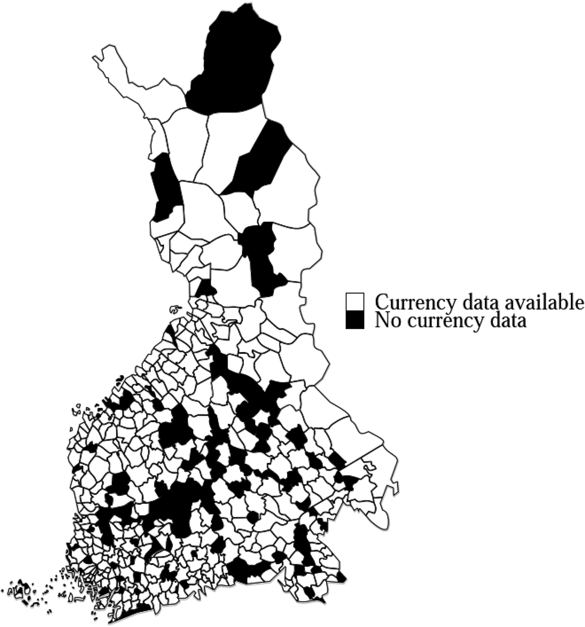
Figure 1. Parishes with currency data available
We begin the analysis by mapping the currencies and analysing their spatial distribution. Figure 2 plots the currency information provided in Böcker's collection. We map the currency shares using local polynomial smoothing to emphasise the relevant spatial patterns.Footnote 2 The Swedish riksdaler (left) was clearly the currency of choice in western and northern Finland, with a sharp dividing line running from the northeastern region of Kainuu, through central Finland to eastern Uusimaa in the south. West of this line, with only a few exceptions, 50 per cent or more of the money used was in riksdalers, while to the east it was roubles.
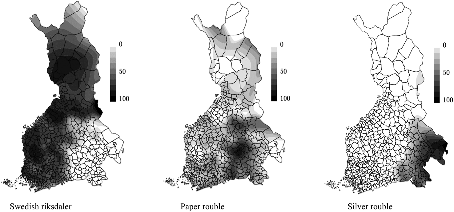
Figure 2. Spatial distribution of currencies in rural Finnish parishes 1833/4, percentage of local money supply
The assignation rouble and Bank of Finland notes can be considered as two forms of the same currency, with Bank of Finland notes denoting the smaller denominations and assignation roubles the larger. In the following, we therefore categorised them as both being forms of ‘paper rouble’.Footnote 3 The paper roubles (middle) were generally confined to the southern coast and the non-coastal regions of Savo and Karelia; but there are also concentrations of assignation roubles in eastern Lapland (to the northeast), and Bank of Finland notes in the southwest area (also known as ‘Finland Proper’). Meanwhile, further up the west coast, in the region of central Ostrobothnia, there were many parishes where paper roubles made up to 50 per cent of the money in circulation – most of this in Bank of Finland notes.
Although generally considered obsolete by this time, according to Böcker's collection the silver rouble was also in circulation; indeed, it made up well over 80 per cent of the local M0 for many parishes in the northeastern part of Viipuri province, and was particularly prevalent in those areas of the southeast that were incorporated into Russia after the wars of 1700–21 and 1741–3. This ‘Old Finland’, as it was known, became reintegrated with the rest of the autonomous Grand Duchy of Finland in 1812.
In addition to the principal currencies, a few anomalies were also reported in Böcker's collection. There was a substantial amount of Norwegian currency (‘Norsk mynt’) in the parishes of Muonio and Enontekiö in western Lapland in the north (up to half of local currency supply). Furthermore, some 0.5–1 per cent of money supply in some Ostrobothnian parishes was in silver riksdaler specie, and in southeastern Finland there were a couple of parishes with up to 15 per cent of M0 in (Russian) gold and platinum coins. We return to these later on.
The regional concentrations of currencies is fairly visible in the maps, but to avoid making sweeping claims based on eyeballing alone, we formally accounted for the clustering. In order to test for the spatial autocorrelation in the data, we calculated the Moran's I values for each currency.Footnote 4 These confirmed what could be seen in the maps; all the currencies – silver rouble (I = 0.519, p < 0.001), paper rouble (I = 0.214, p < 0.001) and Swedish riksdaler (I = 0.464, p < 0.001) – were positively spatially autocorrelated:Footnote 5 they clustered to form areas of (non-)prevalence.
In order to account more specifically for the circulation of currencies, we calculated the Simpson index of diversity. This is a sum of the squared sharesFootnote 6 and describes the likelihood of randomly taking two different currencies (i.e. a note or a coin) from the parish of interest and finding them both to be in the same currency. In the event of unified distribution and three currencies to choose from, the minimum probability is one in three. Because of this, we have rescaledFootnote 7 the index so that the variation is from 0 to 1. As another way of looking at currency concentration, we have plotted the share of the most abundant currency in a parish. The two obviously correlate, but the rescaled Simpson index has lower values. These two are plotted in Figure 3.

Figure 3. Measures of currency clustering: re-scaled Simpson index (left) and share of the most abundant currency (right)
According to these maps, each of the three currencies had areas of particularly high concentration. There are three distinct pockets of riksdaler in western Finland, northern Ostrobothnia and Kainuu, and a fourth area in Lapland; a paper rouble cluster in the central region of southern Savo; and a silver rouble cluster in the northern corner of Viipuri Province. These clusters are rimmed by boundary zones, where currencies are more equally distributed. We detail causes of these patterns in the next section.
V
On a macro-scale, the east–west currency pattern in riksdaler-rouble distribution in Figure 2 is most easily explained by the continuing foreign trade connections with Sweden, and the deficit which characterised this. On the other hand, the annexation of the southeast to Russia in 1721 and 1743 and the subsequent banning of Swedish currency in those areas in 1758 would explain the lack of riksdaler in that region. Further explanations as to why riksdaler continued to circulate after Finland's annexation to Russia include complicated monetary conditions in both Sweden and Russia; an absence of the silver standard; unfavourable exchange rates in the state-led conversion attempts; too few roubles in circulation; thin financial markets; crop failures that drove the rouble out due to grain imports from Russia; and a general lack of trust in the Russian currency. Some authors have argued in favour of Gresham's law, but in an environment of floating currencies it would have required a higher inflation risk of the other currency (in this case, the rouble) which it did not displayFootnote 8 (e.g. Pipping Reference Pipping1961a, Reference Pipping1961b; Kuusterä and Tarkka Reference Kuusterä and Tarkka2011; Kauko Reference Kauko2018; Neovius Reference Neovius1898; Hemminki Reference Hemminki2014).
Except for the explanations involving foreign trade and changes in the national borders, there are no explanations in the literature that might shed light on the within-country distribution of currencies. Even more importantly, there are no explanations as to why the currencies would not spread further afield. One can see from just a cursory glance at Figures 2 and 3, that there are not only spatial clusters of each currency, but also clear boundaries between them in many places. This is most obvious in the riksdaler–rouble boundary of northern Karelia and between the two rouble currencies in eastern Finland. Whatever the explanation for the spatial distribution, it has to account not only for the east–west divides, but also for anomalies such as why two neighbouring parishes might have such starkly different currency conditions and why there are roubles in circulation at places on the west coast, far away from their main area of circulation.
There are not a whole lot of options to choose from as being the likely culprit behind the spatial distribution. There were only limited means for movement of currency in early nineteenth-century Finland. To begin with, until the latter half of the nineteenth century, there were restrictions that hampered the free movement of labour (e.g. Heikkinen Reference Heikkinen1997), although they did not completely prevent all movement (especially when it came to seasonal employment). According to Böcker's collection, there were only a few parishes where over 10 per cent of the local currency was obtained through working outside the parish; these were mainly found by the Russian border in the southeast (most likely due to seasonal work in St Petersburg). Tourism and other movement associated with leisure were too negligible to have had any effect on currency patterns. As discussed earlier, the government was unable to make the rouble the sole currency used in tax collection, and so allowed the continued use of riksdaler in fiscal transactions. This means that fiscal responsibilities did not affect the local choice of currency (Kauko Reference Kauko2018).
These considerations leave trade (both between and within rural parishes and between rural and urban regions) as the most likely vector in currency movement and the most probable factor behind currency agglomeration; neighbouring parishes tended to trade with the same urban centres. Following a mercantile policy, the Swedish administration actively tried to concentrate trade in certain towns and, from the 1400s until their formal dissolution in 1779, rural parishes were each designated a town that they could trade with. These towns also often had the right to engage in foreign trade. In practice, the market regions for each town were determined by transportation opportunities and costs, the demand town merchants had for rural products, and their ability to provide credit to the peasants. In this way, the towns supplied (uniform) currency to rural parishes in exchange for goods and services. Except for fairs – that were organised only a few times a year – trading (in the form of licensed retailing) was forbidden in rural Finland. Households were allowed to purchase goods for their own use outside fairs and towns and it is very probable that these purchases were made locally, keeping the currency circuits regional (Möller Reference Möller1954, pp. 165-9; Alanen Reference Alanen1957, pp. 27-31, 49; Mauranen Reference Mauranen, Jutikkala, Kaukiainen and Åström1980, pp. 436-45; Aunola Reference Aunola1967).
It is fair to assume that the old market regions outlived their ‘official’ lifespan (i.e. beyond 1779), and that they were still having an effect on market patterns in the nineteenth century. There are two reasons to believe this. First of all – whether you call it path dependence, inertia or trust – centuries worth of trade connections would have had a certain inherent stability. As transaction costs were substantial, trade routes were not (and could not) be simply redrawn at will. The second reason, tied to the previous, was that these trade routes were not forced to begin with – they were formed through chains of supply and demand and routed so that transportation costs were, if not minimised, then at least sufficiently low to ensure profitability. As a result, there were known deviations from the state-sanctioned trade connections between a town and its designated rural area. For example, the official market town for parishes in northern Karelia was Loviisa on the southern coast, some 500 kilometres (and weeks’ travel) away. As a consequence, the official urban–rural connections were breached by wandering merchants and the illegal sale of products (Wassholm and Sundelin Reference Wassholm and Sundelin2018; Nevalainen Reference Nevalainen2016, pp. 14-15).
The main analytical difficulty, however, is with determining the geographical scope of these market regions. Tracing individual contacts between farmers and urban buyers of their produce, or between rural suppliers and consumers, is an enormous task even in a more restricted geographical area, let alone across a whole country (e.g. Aunola Reference Aunola1967; Hemminki Reference Hemminki2014). In order to study the trade connections, we have compiled a new dataset of local market prices and use these to estimate the extent and spatial reach of market networks in the nineteenth century. These price data are available at the levels of town and administrative district (kihlakunta) (n = 81), and were originally collected by local officials, who then reported them to the upper echelons of government. The government then used these local prices to create the so-called ‘market price scales’ (markegångpriser), which provided the monetary values for tax payments made in kind. The market price scales are generally considered to be accurate and have closely followed other market indicators (e.g. Jörberg Reference Jörberg1972).Footnote 9 We focused on rye prices (converted into grams of silver) following a wider tradition of analysing grain market integration (e.g. Chilosi et al. Reference Chilosi, Murphy, Studer and Tunçer2013; Federico Reference Federico2007), and we chose rye as it was the most abundantly consumed and traded grain in pre-industrial Finland (e.g. Soininen Reference Soininen1974).
The data used in the present analysis are annual, and cover the years 1812 to 1865. Data availability dictated the beginning of the timespan, while the end date was chosen because it was the last year before the disrupting famine of the 1860s.Footnote 10 We also wanted to focus on the pre-industrial era to better highlight the traditional trade system; after the 1860s the connections between rural parishes and their respective urban trading centres became less of a necessity. This was due to the introduction of railways, investments in interior waterways, increasing industrialisation and economic modernisation, an important part of which was the liberalisation of rural trade in 1859.
In order to estimate the trade networks, we used principal component analysis. Principal component analysis is a dimension reduction technique that is widely used to uncover latent components driving variance patterns in observable variables – in this case, the rye prices in administrational districts and towns.
We used a data-oriented strategy to extract four principal components that together accounted for 78.8 per cent of the price variation. We then rotated the end-result using the varimax method to emphasise the loadings per component, which helped us to interpret the results. The variable loadings (i.e. of locality k to component l) are plotted in Figure 4. The component loading measures the strength of connection between a parish and the estimated principal component, which we interpret as a market region; the larger the loading, the closer the connection between the locality and the market.
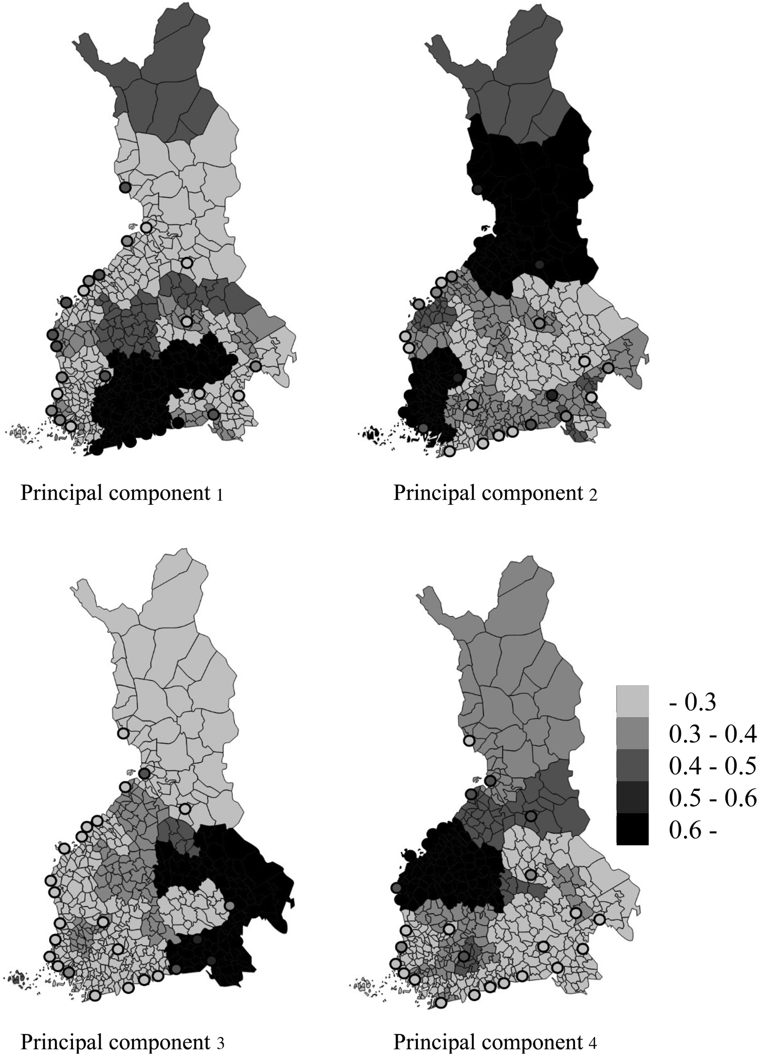
Figure 4. Market regions based on principal component loadings for rye prices, 1812–65
The first component loadings were found mainly in parts of Uusimaa, Häme and southern Savo but they also reached into central Finland and northern Savo. These roughly correspond to the old eighteenth-century Helsinki market region (Ranta Reference Ranta, Jutikkala, Kaukiainen and Åström1980). The loadings of the second component clustered around Finland Proper in the southwest, and the province of Oulu in the north. Substantial loadings are also evident all along the coast, meaning that the second component is the most convenient to interpret, not only as a remnant of the old trading region of Ostrobothnian towns, but also in terms of coastal trade routes.Footnote 11 The third component neatly picks out the old Viipuri market region with localities further inland; these are in accordance with the shift in trade routes that took place in eastern Finland during the early decades of the nineteenth century. Finally, the fourth component depicts the Ostrobothnian market region with a specific emphasis on central and southern Ostrobothnia.
What concerns us here now is the connection between Figures 2 and 4; to what extent was the currency environment determined by these market networks? To assess this, we conducted an econometric exercise to account for the spatial differences in the distribution of currencies. First, we analysed the connection between trade regions and currencies. We did this by employing simple OLS models that used principal component loadings as explanatory variables. In order to account for the spatial autocorrelation in the data, we introduced spatial dependency to the error term (uit=ρWuit+ εit).Footnote 12 This provided a flexible solution to the spatial autocorrelation, doing away with the need to introduce a spatially lagged dependent/independent variable, relaxing the need to explicitly pinpoint the source variable of spatial spillovers (Ward and Gleditsch Reference Ward and Gleditsch2008).
We then introduced a set of control variables. The first of these are distances to certain coastal trade towns.Footnote 13 These gravitational variables accounted for the possibility that rural currency conditions were principally determined by the respective market towns. Secondly, we introduced variables to account for the share of local currency obtained through sales of grain, wood and livestock products (this information was available in Böcker's collection), all of which were tightly clustered in certain parts of the country. This could possibly explain the spatial patterns of certain currencies. Thirdly, we introduced two variables to account for Russian contacts; the share of Russian speakers and Russian tobacco consumed in the rural parishes (also obtained from Böcker's collection). These proxy for the unofficial economic and social connections over the Finno-Russian border, with Russian language facilitating contact, and tobacco being one of the most smuggled good during this period (Nevalainen Reference Nevalainen2016, p. 15).
As our interest lay in the effect of the principal components, we simply forced the set of control variables onto the regression models. Using these variables, we then ran regression models to explain the share of currency i in parish j. These results are reported in Table 1, and we discuss the findings one currency at a time.
Table 1. Explaining the share of different currencies
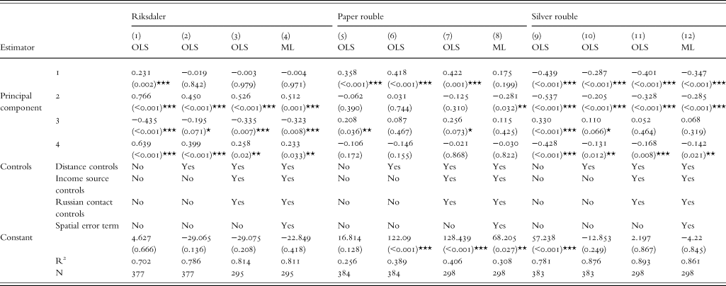
Notes 1. *** denotes statistical significance at 1%, ** at 5%, * at 10% level.
2. The control variables are the following. Urban distance: Euclidian distance to Viipuri, Helsinki, Turku, Kristiinankaupunki, Kaskinen, Vaasa, Pietarsaari, Uusikaarlepyy, Kokkola, Raahe, Oulu and Tornio. Income sources (from Böcker's collection): share of currency obtained through sale of wood products (including tar, firewood, timber), animal products (meat, dairy products) and grain. Russian contacts (from Böcker's collection): share of Russian-speaking population, the extent of use of Russian tobacco (percentage of all tobacco consumed).
3. The maximum likelihood estimated models (4), (8) and (12) include spatial error term (uit=ρWuit+ εit). The R2 values for the spatial models are calculated with standard 1-SSres/SStot formula, using a reduced-form mean. This is a predicted mean of the dependent variable conditional on the independent variables and any spatial lags of the independent variables.
Riksdaler
After controlling for spatial dependency in the errors, and introducing the set of control variables, the second and the fourth principal component had a statistically significant positive effect on riksdaler's circulation, with the statistically significant negative effect from the third component. The strong effect of component two and four on the abundance of riksdaler in model (4) suggests that the trade connections with Sweden via Turku and Ostrobothnian coastal towns supplied Swedish currency to southwestern and western Finland, and that the trade routes not only on the coast but also in the hinterland parishes kept the riksdaler circulating. These principal components also covered the three distinct clusters of riksdaler in western Finland (see Figure 2). The positive effect persisted when controlling for distance to the coastal towns. It also persisted when controlling for the importance of wood-based products in providing currency. The latter is important, as wood products (especially tar and timber) were of substantial economic importance in many of the parishes in the riksdaler part of the country.
The role of the market regions was most visible in the northeastern region of Kainuu. At the sharp boundary between the second and third principal components, the riksdaler–rouble boundary was equally sharp.
Using the designated variables, we were able to account for over 81 per cent of the spatial variation in the distribution of riksdalers. This is an extremely high figure, as in a cross-sectional data we cannot use fixed effects to account for parish heterogeneities.
In total, findings imply that the west of Finland had an integrated economic system based on the Swedish riksdaler.
Before moving on, it is worth noting that the last places where the riksdaler was being used before its final disappearance in the 1850s were the remote corners of northern Finland (Myllyntaus Reference Myllyntaus, Jutikkala, Kaukiainen and Åström1980, p. 341). It is therefore plausible that, to some extent, riksdalers were relics already in the early nineteenth century, especially in the economic hinterlands. The sporadic presence (albeit with a low share) of silver riksdaler specie in some parishes in western Finland could be interpreted in similar fashion; widely considered obsolete at the time, these coins were probably relics from the eighteenth century, retained most likely for their silver content (Talvio Reference Talvio2003, pp. 24-5; see also Schauman Reference Schauman1967, pp. 182–3 for an anecdotal account on the relic interpretation).
Paper roubles
The distribution of the paper roubles is the trickiest one to reduce to the independent variables used in this study. Indeed, models 5-8 were only able to account for roughly 30-40 per cent of the spatial variation in this currency's distribution. The Helsinki market region, spanned by the first principal component, was in strong positive association with the spatial prevalence of the paper rouble in models 5-7. This is logical as the Bank of Finland, which supplied small denomination roubles, had its only office in Helsinki. Furthermore, after Helsinki was made the capital of Finland (in 1812), the overall economic geography of the country shifted to become more Helsinki-oriented (Nummela Reference Nummela and Haapala2018). This naturally connected Helsinki-bound trade with the official currency – the paper rouble. Another route for the paper rouble spread was provided by the connections to southeastern Finland, especially to town of Viipuri. After the province of Viipuri (in the southeast) was restored to Finland in 1812, many parishes in eastern Finland began trading again with the town of Viipuri and other towns in the area (Alanen Reference Alanen1957, pp. 148-53; Mauranen Reference Mauranen, Jutikkala, Kaukiainen and Åström1980, pp. 441, 436; Ranta Reference Ranta, Jutikkala, Kaukiainen and Åström1980) and, as we might expect, we observe a more complete shift from riksdaler to rouble in parishes closer to Viipuri than in parishes further away.
The first principal component does not have a statistically significant effect on the distribution of the paper rouble when the spatial clustering in the error term is accounted for. This apparently stems from the correlation between the distance to Viipuri and the first principal component. After dropping the one, the other retains its statistical significance with the expected sign (positive for the principal component, negative for the distance).Footnote 14
The way the paper rouble extends into the western Finland, as clearly seen in Figure 2, coincides with similar, albeit weak east–west patterns in most of the principal components (especially in component 3). The heterogeneity and the relative weakness of these contacts provide a plausible reason why the riksdaler and roubles had such a distinct east–west division. The east–west component loadings were often between 0.3 and 0.4 (especially in principal components 2 and 3), so the low proportion of paper roubles in these western areas (mainly between 10 and 20 per cent) is in line with the strength of respective east–west economic connections. The negative effect the second principal component has is in line with these; the paper rouble was unable to penetrate western Finland.
Interestingly, there are coastal parishes in the west where the share of paper roubles was very high. These are restricted particularly to the immediate surroundings of Kokkola, Pietarsaari and Uusikaarlepyy, where the paper rouble (mostly Bank of Finland notes) reached 40 to 50 per cent of the local M0. This pattern corresponds to the coastal towns’ high loadings to the first principal component. In comparison, the parishes only slightly further away had a much smaller share of paper roubles in their money supply. Accordingly, the fourth principal component, which spans these regions, does not have any significant effect on the distribution of the paper rouble; the west coast pockets of Bank of Finland notes plausibly originated from trade which targeted Helsinki and had little connection to trade within the Ostrobothnian area.
Silver roubles
Due to its limited spatial reach, the distribution of the silver rouble is fairly easily explained with the variables of choice; R2 values are close to 90 per cent. We surmise from the regression results that the silver rouble was a relic and used in poorer secondary markets and/or in the economic hinterland of not only Finland but also elsewhere in Imperial Russia (see also Talvio Reference Talvio2003, p. 24). Like silver riksdaler specie coins in the Ostrobothnia, reported gold and platinum currencies in a few parishes in these same regions also tally with the relic explanation (see, e.g., Talvio Reference Talvio2003, p. 30).
The regions around Lake Ladoga (on both the Finnish and Russian sides of the border) are known to have been poor (Nummela Reference Nummela and Haapala2018; Nevalainen Reference Nevalainen2016, pp. 28, 30). Furthermore, in the parishes with the majority of their M0 in silver roubles, trade within Finland was not a significant source of income (Soininen Reference Soininen1974, p. 362). While this possibly hampered the economic development of the region, it importantly prevented the flow of other currencies from displacing the silver rouble. This would also explain why none of the principal components load positively to models (11) or (12).
This does not mean, however, that trade did not play its part in shaping the currency conditions in these parts of the country: the silver rouble in Finland could simply have been a spillover from cross-border trade with the Russian regions around Lakes Ladoga and Onega. There were deep historical and cultural connections to these regions (Vuorela Reference Vuorela1976; Sarmela Reference Sarmela1994; Kokkonen Reference Kokkonen2002, pp. 35, 192–201, 345),Footnote 15 and because the border had changed so much over previous centuries, it is likely that people living in this area accommodated the risks involved by establishing stable economic connections across the region whether or not there was a border between them (Ranta Reference Ranta1986). The existence of Norwegian currency in the western Lapland can probably be explained with a similar logic: the national borders did not hamper economic connections, especially in the economic peripheries.
Our discussion provides a tangible explanation for the spatial agglomeration of the currencies by establishing that parishes in the same market region used a roughly uniform medium of exchange. We are, however, compelled to make a few disclaimers before concluding.
First of all, when assessing these patterns, it is important to keep in mind the fact that the principal components were estimated from time-series data, while currencies were only known from a single cross-section. To check the sensitivity of our results with regard to the precise time period for which these components are estimated, we also conducted the principal component analysis with data from the period 1812–33 (in other words, the years directly preceding our cross-sectional currency data). The principal components were found to be qualitatively identical, but their extraction was less conclusive; several locations loaded strongly to several components and the first and second components in Figure 4 were found to be essentially joined together, though still maintaining the east–west pattern of price integration. This kind of result is to be expected, as low sample sizes are known to hamper the extraction of principal components.
This finding reduces our concerns about endogeneity issues; beforehand, we cannot be sure whether uniform currency facilitated trade or if it was the other way around. Because we lack longitudinal currency data we cannot assess Helleiner's (Reference Helleiner2003) hypothesis, which connects market integration with currency unification, so we cannot quantitatively assess whether a unified currency environment was essential for markets to become integrated. Nevertheless, we consider that the evidence presented here means the answer is ‘most likely not’, and that the causality probably runs in the other direction. We base this on the fact that we found the same market regions already in place before the date of our currency cross-section (1833/34) and these furthermore aligned with the trade networks in the centuries before (Ranta Reference Ranta1980). The fact that even under the eighteenth-century Swedish currency system (which was considerably more homogenized than the 1809-40 Finnish system) Finland was characterised by regionally separated market regions implies that trade networks transported currencies, not the other way round. The direction of causality is furthermore showcased in the spread of roubles to eastern Finland after the southeastern corner was re-annexed to Finland in 1812 – the currency environment changed in line with the changing trade possibilities.
A cautionary note should be sounded in that the market regions are imperfectly measured. We used prices of rye to map the regions, but this might well not account for trade patterns of other goods. It might apply especially to goods that were sold mainly to towns, as opposed to others that were purchased for personal consumption more locally. Furthermore, there might be regional and currency-specific differences as to whether trade was conducted using currency or by barter or by account debt.
Finally, we emphasise that the research setting is suggestive in the face of a lack of individual-level micro-data. Parishes are not the best statistical units for causative analysis, and to move beyond the simple association analysis put forward here, we would need more detailed individual-level trader data to verify the conclusions drawn.
VI
This study has focused on the spatial differentiation of currencies within rural Finland during the first half of the nineteenth century. We have shown that different currencies were clustered in specific areas of the country. Based on regression analysis, we showed that currencies clustered within certain ‘market regions’, that were rural areas in which people traditionally travelled to market towns to sell their products, and where people locally purchased goods for their own consumption. Our findings suggest that these kinds of connections were vital in determining the spread and circulation of currencies.
How does our article contribute to a more general historical understanding of multi-currency regimes? Firstly, using Finnish data we have shown that only a few places had a uniform distribution of different notes and coins. The places where different currencies were distributed more or less uniformly were rural hinterlands and those lying in the transition zones between the main clusters of currencies. We do not overtly want to push the generality of these results, but we are intrigued by what they suggest: genuine multi-currency systems – where economic agents simultaneously used a number of currencies – might have actually been quite rare. The Finnish experience appears to highlight the fact that even if, on aggregate, the country had an economic system characterised by several different currencies, currency conditions might nevertheless have been fairly homogenised at the local level.
Secondly, the spatial extent of currencies was largely determined by the market connections between towns and rural parishes on the one hand, and between and within rural parishes on the other. As is to be expected from theoretical considerations emphasising the homogenisation of currency to minimise transaction costs, we observed a striking uniformity of currency within these market regions.
Our article suggests two principal reasons why ‘natural’ market diffusion could not produce a homogeneous currency environment in nineteenth-century Finland. Firstly, historically separated markets had substantial inertia: Finland did not constitute a uniform market region during the period of our study. This prevented free flow of currencies from one place to another, and therefore helped maintain the regional nature of the currency systems.
Secondly, the situation was aggravated by an insufficient supply of the paper roubles. The paper rouble replaced the riksdaler to a substantial extent in those places it reached through market channels. Over time, the east–west connections, although weak, allowed the paper rouble to leak westwards, though the main route for roubles to reach the west coast seems to have been via maritime connections with Helsinki.
Homogenisation of the national currency environment did not happen without a strong national intervention that was able to overrule the inertia caused by historical market networks and an insufficient rouble supply. This did not happen until the early 1840s when the Russian state instigated widespread currency reform.


 Open access