


Impact Statement
Clustering offshore wind farms leads to large-scale aerodynamic interactions, negatively impacting their power production. However, wind farm design and siting tools cannot accurately capture these interactions. We use large-eddy simulations to study the physical processes that impact the performance of neighbouring wind farms. We find that a wind farm wake can reduce the power production of turbines throughout the downstream wind farm, and not just of turbines in the first row. Furthermore, we demonstrate that the flow inside and around the downstream farm is strongly affected, revealing that wind farms affect flow features beyond the wind farm scale. In particular, we find that the vertical entrainment fluxes above the downstream wind farm are increased, which leads to increased wake recovery inside and behind the downstream wind farm.
1. Introduction
The number of wind farms is increasing due to the growing demand for renewable energy. In 2020 the total installed capacity in Europe was  $220 \ \mathrm {GW}$, and an additional $105 \ \mathrm {GW}$ is expected in the coming five years (Reference Komusanac, Brindley, Fraile and RamirezKomusanac, Brindley, Fraile, & Ramirez, 2021). Especially in offshore regions, wind farms are often clustered, as the space in shallow water depths is limited (Reference NygaardNygaard, 2014; Reference Platis, Hundhausen, Mauz, Siedersleben, Lampert, Bärfuss and BangePlatis et al., 2020). Furthermore, the transport of the generated electricity is facilitated by clustering wind turbines. However, closely spaced wind farms negatively affect each other's performance as wind farm wakes, i.e. regions of velocity deficit and increased turbulence intensity, have been observed to persist far downstream of wind farms (Reference Cañadillas, Foreman, Barth, Siedersleben, Lampert, Platis and NeumannCañadillas et al., 2020; Reference Schneemann, Rott, Dörenkämper, Steinfeld and KühnSchneemann, Rott, Dörenkämper, Steinfeld, & Kühn, 2020). The wind farm wake development depends on the prevailing atmospheric conditions, as well as the size and layout of the wind farm (Reference Cañadillas, Beckenbauer, Trujillo, Dörenkämper, Foreman, Neumann and LampertCañadillas et al., 2022; Reference Maas and RaaschMaas & Raasch, 2022; Reference NygaardNygaard, 2014; Reference Platis, Hundhausen, Mauz, Siedersleben, Lampert, Bärfuss and BangePlatis et al., 2020; Reference Schneemann, Rott, Dörenkämper, Steinfeld and KühnSchneemann et al., 2020), such that our fundamental understanding of wind farm wakes is still limited and is not well captured in wind farm design and siting tools (Reference Porté-Agel, Bastankhah and ShamsoddinPorté-Agel, Bastankhah, & Shamsoddin, 2020; Reference Stieren and StevensStieren & Stevens, 2021). This emphasizes the importance of studying the impact of wind farm wakes on downstream wind farms.
To study long-distance wakes behind wind farms, measurements or numerical simulations need to cover a large spatial area. As an example, wind farm wakes have been observed with satellite synthetic aperture radar (SAR) measurements (Reference Ahsbahs, Nygaard, Newcombe and BadgerAhsbahs, Nygaard, Newcombe, & Badger, 2020; Reference Christiansen and HasagerChristiansen & Hasager, 2005; Reference Djath and Schulz-StellenflethDjath & Schulz-Stellenfleth, 2019; Reference Hasager, Vincent, Badger, Badger, Bella, Peña and VolkerHasager et al., 2015). Recently, Reference Schneemann, Rott, Dörenkämper, Steinfeld and KühnSchneemann et al. (2020) used SAR measurements to detect wind farm wakes up to  $55 \ \mathrm {km}$ downstream of a wind farm cluster with more than $250$ turbines in a stably stratified atmosphere. The average velocity deficit $55 \ \mathrm {km}$ downstream of the cluster was observed to be $21\,\%$, with clear transition regions separating wake and free flow. Wind farm wakes are longer in stable atmospheric conditions for which the turbulence intensity is low. In neutral and especially unstable conditions, the turbulence intensity is higher, such that the wake recovery is faster (Reference Cañadillas, Foreman, Barth, Siedersleben, Lampert, Platis and NeumannCañadillas et al., 2020; Reference Schneemann, Rott, Dörenkämper, Steinfeld and KühnSchneemann et al., 2020). The SAR observations by Reference Christiansen and HasagerChristiansen and Hasager (2005) of wind farms with up to 80 wind turbines report an average velocity deficit of $2\,\%$ at a downstream distance of $5 \ \mathrm {km}$ for unstable and of $20 \ \mathrm {km}$ for near-neutral conditions. The differences compared with the study of Reference Schneemann, Rott, Dörenkämper, Steinfeld and KühnSchneemann et al. (2020) suggest that the atmospheric conditions and the wind farm layout influence the recovery rate of wind farm wakes. This hypothesis was confirmed by Reference Platis, Hundhausen, Mauz, Siedersleben, Lampert, Bärfuss and BangePlatis et al. (2020) who used airborne data to study long-distance wakes (Reference Platis, Siedersleben, Bange, Lampert, Bärfuss, Hankers and EmeisPlatis et al., 2018, Reference Platis, Hundhausen, Mauz, Siedersleben, Lampert, Bärfuss and Bange2020). For wind farms with different layouts and sizes in the North sea, they reveal that a smaller interturbine spacing results in a lower velocity directly behind the wind farm and an increased wake length.
In contrast to field measurements, numerical simulations make it possible to study the flow under well-controlled and reproducible conditions. Simulations allow for a better physical understanding of the development of wind farm wakes and how atmospheric flow conditions affect this process. The study of wind farm wakes and their influence on downstream positioned wind farms requires large numerical domains. Consequently, simulations of the interaction between large-scale wind farms have primarily been performed in mesoscale models using wind farm parameterizations (Reference Fitch, Olson, Lundquist, Dudhia, Gupta, Michalakes and BarstadFitch et al., 2012; Reference Mayol, Saulo and OteroMayol, Saulo, & Otero, 2021). Reference Lundquist, DuVivier, Kaffine and TomaszewskiLundquist, DuVivier, Kaffine, and Tomaszewski (2019) used mesoscale simulations to show that wind farm wakes can have a significant impact on the performance of downstream farms. Additionally, Reference Lundquist, DuVivier, Kaffine and TomaszewskiLundquist et al. (2019) compared predicted and actual capacity factors of situations with and without wind farm wake effects to show the economic consequences of wake effects. Recently, Reference Akhtar, Geyer, Rockel, Sommer and SchrumAkhtar, Geyer, Rockel, Sommer, and Schrum (2021) applied mesoscale simulations to analyse the annual wind speed variations in the North Sea over 10 years. They conclude that wind farm wake effects can reduce the capacity factor by approximately  $20\,\%$ when wind farms are placed within $7 \ \mathrm {km}$ of each other.
Mesoscale simulations and Reynolds-averaged Navier–Stokes (RANS) are often used to validate and optimize engineering models (Reference Platis, Hundhausen, Mauz, Siedersleben, Lampert, Bärfuss and BangePlatis et al., 2020). Examples of engineering models used to model wind farm wakes can be found in Reference EmeisEmeis (2018), Reference Nygaard, Steen, Poulsen and PedersenNygaard, Steen, Poulsen, and Pedersen (2020), Reference Stieren and StevensStieren and Stevens (2021) and Reference Cañadillas, Foreman, Barth, Siedersleben, Lampert, Platis and NeumannCañadillas et al. (2020). However, the horizontal resolution in mesoscale simulations is often larger than the wind turbine diameter (Reference Baidya-RoyBaidya-Roy, 2011; Reference Carvalho, Rocha, Gómez-Gesteira and SantosCarvalho, Rocha, Gómez-Gesteira, & Santos, 2012; Reference DraxlDraxl, 2012; Reference Siedersleben, Platis, Lundquist, Djath, Lampert, Bärfuss and NeumannSiedersleben et al., 2020), and smaller domain sizes are required to obtain finer resolution. Furthermore, RANS simulations have been used to study the wake behind wind farms and the interaction between wind farms, revealing the importance of the Coriolis force on the relevant scales for wind farm interaction (Reference Hansen, Réthoré, Palma, Hevia, Prospathopoulos, Peña and VolkerHansen et al., 2015; Reference van der Laan, Hansen, Sørensen and Réthorévan der Laan, Hansen, Sørensen, & Réthoré, 2015; Reference van der Laan and Sørensenvan der Laan & Sørensen, 2017). In contrast to RANS and mesoscale simulations, more detailed large-eddy simulations (LES) capture temporal fluctuations and resolve large-scale flow features in an atmospheric boundary layer (ABL), while the small-scale turbulence is parameterized using a subgrid scale model. Also, LES have been shown to accurately capture wind turbine wake interaction in an unsteady anisotropic turbulent atmosphere. However, due to high computational cost, most LES have focused on individual wind turbines or wind farms, not the interaction between wind farms (Reference Porté-Agel, Bastankhah and ShamsoddinPorté-Agel et al., 2020; Reference Stevens and MeneveauStevens & Meneveau, 2017). Recently, Reference Maas and RaaschMaas and Raasch (2022) performed LES to study wind farm wakes in the German Bight. They observe that wind farm wakes are longer when the ABL is lower or when the interturbine spacing in the farm is smaller. They find that, depending on the atmospheric conditions, the velocity deficit of the wind farm wake can be observed up to  $100 \ \mathrm {km}$ behind the wind farm, while the enhanced turbulence intensity can be observed up to $20 \ \mathrm {km}$ downstream.
In this study we use LES to study the impact of a wind farm wake on a downstream wind farm. For this purpose, we perform LES and systematically increase the distance between two identical wind farms, each consisting of 72 wind turbines. Representative for existing and planned wind farm clusters in the North Sea, the distance between the wind farms is varied between  $5$ and $15 \ \mathrm {km}$ (Reference Cañadillas, Foreman, Barth, Siedersleben, Lampert, Platis and NeumannCañadillas et al., 2020; Reference Maas and RaaschMaas & Raasch, 2022). We note that these distances also correspond to the optimal wind farm spacing of 4 to 14 km suggested by Reference Frandsen, Barthelmie, Pryor, Rathmann, Larsen, Højstrup, Nielsen and ThoegersenFrandsen et al. (2005). Considering two identical wind farms allows us to directly compare the power production of turbines in the first and the downstream wind farm. Only in this way we can study the impact of the wind farm wake on the power production of turbines in the downstream wind farm. Furthermore, we study the impact of the wind farm layout on the interaction between wind farms by considering aligned and staggered wind farms. This allows us to show, in agreement with previous studies (Reference Platis, Hundhausen, Mauz, Siedersleben, Lampert, Bärfuss and BangePlatis et al., 2020), that the observed interaction between wind farms depends on the wind farm layout. The simulations are performed for neutral ABL conditions driven by a geostrophic wind. Such an ABL configuration is representative for cloudy days, near sunset or sunrise, and for ABLs formed offshore (Reference Högström, Hunt and SmedmanHögström, Hunt, & Smedman, 2002). The remainder of the manuscript is structured as follows. In § 2 we introduce the LES modelling framework and the considered wind farm layout. In § 3 we present the results, and the conclusions are discussed in § 4.
2. Large-eddy simulations
The simulations are performed using the LES code initially developed by Reference Albertson and ParlangeAlbertson and Parlange (1999), which is continuously updated and tested (Reference Gadde, Stieren and StevensGadde, Stieren, & Stevens, 2021; Reference Stieren, Gadde and StevensStieren, Gadde, & Stevens, 2021). The governing equations are the filtered continuity equation and momentum-conservation equation,
 $$\begin{gather} \partial_i \tilde{u}_i = 0, \end{gather}$$
 $$\begin{gather}\partial_t \tilde{u}_i + \partial_j ( \tilde{u}_i \tilde{u}_j ) = {-}\partial_i \tilde{p}^{{\ast}} - \partial_j \tau_{ij} - \epsilon_{ijk}\, f_{c,j} (\tilde{u}_k -G_k) + \tilde{f}_i , \end{gather}$$
where  $u$ is the velocity and $i=1,2,3$ correspond to the streamwise ( $x$,
$x$, $u$), spanwise ( $y$,
$y$, $v$) and vertical ( $z$,
$z$, $w$) direction and component, respectively. The tilde indicates that a filtered velocity field is considered, and $\delta _{ij}$ is the Kronecker delta. The viscous stresses are neglected as we consider very high Reynolds number atmospheric flow, and the subgrid stresses (SGS) are modelled through $\tau _{ij} = \widetilde {u_i u_j}-\tilde {u}_i\tilde {u}_j$. The trace of the SGS stress tensor is absorbed into the filtered modified pressure $\tilde {p}^{{\ast }}= \tilde {p}/\rho _0-p_{\infty }/\rho _0+\tau _{kk}/3$, where $\tilde {p}$ is the pressure and $\rho _0$ is the air density. The SGS deviatoric stress is modelled using the anisotropic minimum dissipation model (Reference Abkar, Bae and MoinAbkar, Bae, & Moin, 2016) with a Poincaré constant of $C_i=1/\sqrt {12}$ in horizontal and $C_i=1/\sqrt {3}$ in vertical direction, respectively. A mean pressure gradient $\partial _i p_{\infty }$, which is related to the geostrophic wind velocity as $G_i=-\epsilon _{ij3}\partial _j p_{\infty }/(\rho _0 f_c)$, drives the flow in the ABL ( $\epsilon _{ijk}$ denotes the alternating unit tensor). The Coriolis parameter is given by $f_c=(0,2 \varOmega \cos (\varPhi ),2 \varOmega \sin (\varPhi ))$ with the rotation angular speed $\varOmega$ and latitude $\varPhi$.
The wind turbines are modelled as actuator disks (Reference Calaf, Meneveau and MeyersCalaf, Meneveau, & Meyers, 2010). The thrust force exerted by a wind turbine on the flow is approximated as  $F_t = - \frac {1}{8} \rho _0 C_T' \langle \bar {u}^T\rangle _{{disk}}^2 {\rm \pi}D^2$, where $\langle \bar {u}^T\rangle _{{disk}}$ is the disk-averaged velocity and $C_T'=C_T/(1-a)^2$ includes the thrust coefficient $C_T = 0.75$ and the induction factor $a=0.25$. The streamwise and spanwise components of the turbine force are included in (2.2) as $\tilde {f}_1=F_t \cos \phi$ and $\tilde {f}_2=F_t \sin \phi$ with the angle $\phi$ between the actuator disk and the $x$-axis. Reference Wu and Porté-AgelWu and Porté-Agel (2011) demonstrated that the actuator disk model provides an adequate representation of the overall wake structure behind the wind turbines starting from three diameters downstream of the turbine. This agreement was confirmed by Reference Stevens, Martínez-Tossas and MeneveauStevens, Martínez-Tossas, and Meneveau (2018), who validated the actuator disk model and actuator line model against experimental data. Here, we also use the actuator disk model correction factor introduced by Reference Shapiro, Gayme and MeneveauShapiro, Gayme, and Meneveau (2019). Therefore, the actuator disk model is considered to be sufficiently accurate to capture the large-scale flow phenomena studied here.
Time integration is performed using a second-order accurate Adams–Bashforth scheme. Derivatives in the vertical direction are calculated using a second-order central finite difference scheme, and in the horizontal directions a pseudospectral method is applied. The computational domain is discretized with  $n_x$, $n_y$ and $n_z$ points in streamwise, spanwise and vertical directions. The grid sizes in horizontal direction are $\varDelta _x = L_x/n_x$, $\varDelta _y = L_y/n_y$, where $L_x$ and $L_y$ are the dimensions of the computational domain. The computational grid is vertically staggered such that the first vertical velocity plane is located at the ground and the first grid point for $u$,
$u$,  $v$ and $\theta$ is located at $z/2$. No-slip and free-slip boundary conditions with zero vertical velocity are used at the top and bottom boundaries, respectively. The wall shear stress $\tau _{i3|w}$ at the ground is modelled using the Monin–Obukhov similarity theory (Reference MoengMoeng, 1984) such that $\tau _{i3|w} = - [{\tilde {u}_r \kappa }/{\ln (z/z_{0})} ] ({\tilde {u}_i}/{\tilde {u}_r})$, where $z_0$ is the roughness length, $\kappa$ is the von Kármán constant and $\tilde {u}_r=\sqrt {\tilde {u}^2+\tilde {v}^2}$ is the filtered velocity magnitude at the first grid level (Reference Bou-Zeid, Meneveau and ParlangeBou-Zeid, Meneveau, & Parlange, 2005). We use a surface roughness of $z_0=0.002$ m, which is a typical value for offshore conditions (Reference Golbazi and ArcherGolbazi & Archer, 2019).
A schematic of the considered wind farm configuration is shown in figure 1. The main simulation domain includes two wind farms consisting of  $12\, {\times}\, 6$ wind turbines. The upstream wind farm is positioned $7$ km downstream of the inflow region, and the distance between the wind farms is varied from $5$ to $15 \ \mathrm {km}$, see table 1. The wind turbines have a diameter of $D=120\ \mathrm {m}$ and the hub height is $z_h=100\ \mathrm {m}$. The distance between the wind turbines is $s_x=7D$ and $s_y=5D$ in the streamwise and spanwise directions, respectively. The wind turbines are either fully aligned with the incoming wind or in a staggered layout. This results in a wind farm length $L_{{Wf}}=9.24 \ \mathrm {km}$ and a wind farm width $W_{{Wf}}=3.12 \ \mathrm {km}$ for the aligned layout and $W_{{Wf}}=3.42\ \mathrm {km}$ for the staggered layout. In this work we use ${Wf}$ as an abbreviation for a wind farm. Here, $Wf1$ and $Wf2$ denote the upstream and downstream wind farm, respectively. Both the wind farm and the precursor domain have a size of $L_x=54\ \mathrm {km}$, $L_y=7.2\ \mathrm {km}$ and $L_z=4.0$ km, which is discretized on a $1800 \times 480 \times 480$ grid. The vertical resolution is $5\ \mathrm {m}$ up to a height of $1.5\ \mathrm {km}$ and grid stretching is applied above. The actuator disks are resolved with 24 grid points in vertical and 8 grid points in spanwise directions. This resolution has been shown to be sufficient by Reference Wu and Porté-AgelWu and Porté-Agel (2013) and Reference Stevens, Martínez-Tossas and MeneveauStevens et al. (2018).

Figure 1. Schematic of the computational domain, showing the wind farm layout and the fringe layer configuration. The distance between the farms  ${\rm \Delta} x_{{Wf}}$ is varied from $\textit{5}$ to $\textit{15} \ \mathrm {km}$.
Table 1. The case names are constructed as follows: the first part denotes the layout and the second part denotes the distance between the wind farms.

Realistic atmospheric inflow conditions are generated by the concurrent precursor method (Reference Stevens, Graham and MeneveauStevens, Graham, & Meneveau, 2014). This approach samples flow data from a periodic turbulent ABL simulation performed in a precursor domain. The sampled data is introduced as an inflow condition into a fringe region of the wind farm simulation domain, see figure 1, and we apply shifted periodic boundary conditions to reduce the effect of persistent large-scale structures in the atmospheric inflow (Reference Munters, Meneveau and MeyersMunters, Meneveau, & Meyers, 2016). Nevertheless, some remnants of these large-scale structures are still visible in the results.
Furthermore, we apply a proportional-integral controller (Reference Allaerts and MeyersAllaerts & Meyers, 2015; Reference Sescu and MeneveauSescu & Meneveau, 2014) to guarantee that the planar-averaged wind angle at hub height is  $0^{\circ }$ and aligned with the wind farm geometry. In addition, as the wind direction changes with height, we use a symmetric fringe function (Reference Stieren, Gadde and StevensStieren et al., 2021). The simulations are performed with the Earth's rotation angular speed $\varOmega =7.3 \times 10^{-5}$ rad s $^{-1}$ and for a latitude $\varPhi =52^{\circ }$, which is representative for the Dutch North Sea area. The geostrophic-wind velocity $G$ is assumed to be constant, thus representing barotropic conditions, with a value of $11$ m s $^{-1}$. The direction of the geostrophic-wind velocity is from west to east (Reference Howland, Ghate and LeleHowland, Ghate, & Lele, 2020b). The simulations are started from an initial wind profile that is set equal to the geostrophic wind, and uniformly distributed random perturbations are added below $50 \ \mathrm {m}$ to spin up turbulence. The perturbations have an amplitude of $3\,\%$ of the geostrophic wind. These spin-up simulations are performed in a domain size of $L_x=27\ \mathrm {km}$, $L_y=3.6\ \mathrm {km}$ and $L_z=4.0$ km. After $8.7$ hours a quasi-steady state is reached and then the domain size is increased to $L_x=54\ \mathrm {km}$, $L_y=7.2\ \mathrm {km}$ and $L_z=4.0\ \mathrm {km}$, which is possible due to the periodic boundary conditions. Subsequently, the precursor and wind farm simulations are continued concurrently for two additional hours. The statistical data is collected over five hours, corresponding to approximately three flow-through times.
Validations of the employed domain length and width, as well as the considered averaging time, are provided in the supplementary material (available at https://doi.org/10.1017/flo.2022.15). For example, we performed an additional simulation in a wider domain to verify that the presented findings are not affected by the domain size. We find that the wind farm power production of the upstream and downstream farms is reduced by 1.5 % when the domain size is doubled due to the decreased flow blockage. It is important to emphasize that this affects the upstream and downstream farms in a similar way and does not affect the main physics much. The supplementary material further includes a colour-blind friendly version of the colour plots shown in this manuscript.
2.1 Boundary layer characteristics
Figure 2 presents the time and planar-averaged atmospheric inflow conditions obtained from the precursor simulation. The horizontal velocity magnitude  $\langle \bar {v}_h\rangle =\langle \sqrt { \bar {u}^2+\bar {v}^2}\rangle$, where $\langle$ $\rangle$ is the planar average and the overbar represents the temporal average, is shown in figure 2(a). The tilde representing filtering is dropped in the remainder of the paper for simplicity. The velocity at hub height is $9.5 \ \mathrm {m}\ \mathrm {s}^{-1}$ and the highest velocity, due to the formation of a weak low-level jet, is $11.4 \ \mathrm {m}\ \mathrm {s}^{-1}$ at $0.93\ \mathrm {km}$. The horizontal turbulence intensity is defined as $\langle {\overline {TI}} \rangle =\langle \sqrt {\overline {u'^2}+\overline {v'^2}}\rangle /\langle \bar {v}_h \rangle$ and is $9\,\%$ at hub height. The vertical profile of the turbulence intensity is presented in figure 2(b). Figure 2(c) shows the planar-averaged vertical momentum flux, which is defined as $\langle \bar {\tau } \rangle =\langle \sqrt {(\overline {u'w'})^2 + (\overline {v'w'})^2} \rangle$ with $\overline {u'w'}=\overline {uw}+\overline {\tau _{xz}}-\bar {u} \bar {w}$ and $\overline {v'w'}=\overline {vw}+\overline {\tau _{yz}}-\bar {v} \bar {w}$. The boundary layer height is $z_i=1.73 \ \mathrm {km}$, which is defined as the height where the mean stress is 5 % of its surface value ( $z_{0.05}$) followed by a linear extrapolation, i.e. $z_i = z_{0.05}/0.95$ (Reference Kosović and CurryKosović & Curry, 2000). The wind angle $\langle \bar {\alpha } \rangle =\ \tan ^{-1}(\langle \bar {v} \rangle /\langle \bar {u} \rangle )$ as a function of height is shown in figure 2(d), which shows that $\langle \bar {\alpha } \rangle$ changes from $1.02^{\circ }$ at $z_h - D/2$ to $\langle \bar{\alpha} \rangle = -0.91^{\circ }$ at $z_h + D/2$, resulting in a wind veer over the vertical extent of the rotor of $2^{\circ }$.

Figure 2. Temporally and horizontally averaged inflow conditions. (a) Horizontal velocity magnitude, (b) turbulence intensity, (c) vertical momentum flux and (d) wind angle as a function of height. The shaded area indicates the vertical extent of the wind turbines.
3. Results
3.1 Flow adjustment in and around the wind farms
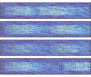
Figure 3(a) shows the instantaneous horizontal velocity magnitude at hub height for case stag-10 km. The figure shows that the wakes meander downstream and form a wind farm wake, creating the inflow condition for the downstream wind farm. We also refer to the corresponding movie in the supplementary material. Figure 3(b) displays the velocity  $1D$ downstream of the last row of the upstream wind farm. The strongest wake deficits are in the centre, suggesting that energy is entrained from the sides as the wake deficit is less pronounced at the edges. Above the wind turbines, it can be observed that the flow is rotated in the clockwise direction, see also figure 2(d). This effect is even more visible in figure 3(c), which shows the flow $1D$ behind the last row of the downstream wind farm. A comparison between figures 3(b) and 3(c) shows that the velocity $1D$ behind the downstream wind farm is lower than $1D$ behind the upstream farm. This indicates that the velocity deficit is stronger behind the downstream farm. This effect is further analysed below, see in particular figure 6(a), which analyses the wind strength throughout the wind farm.

Figure 3. Instantaneous horizontal velocity magnitude  $v_h=\sqrt {u^2+v^2}$ (a) at hub height, (b) $1D$ behind the last row of the upstream wind farm and (c) $1D$ behind the last row of the downstream farm. The positions of the wind turbines are marked by (a) black lines and (b,c) circles. Circles indicate the spanwise-vertical location of the turbines for uneven (grey) and even (black) turbine rows.
Figure 4(a–c) show the time-averaged horizontal velocity magnitude at hub height for the staggered wind farms that are separated by  $5 \ \mathrm {km}$, $10 \ \mathrm {km}$ and $15 \ \mathrm {km}$, respectively. Obviously, the flow inside the upstream wind farm is nearly identical for all cases, while the figure clearly shows that the velocities in the downstream wind farm are higher when the distance between both farms is increased from $5$ to $15 \ \mathrm {km}$. The wind farm wake is most intense directly behind the farm where it spans the total width of the wind farm. Farther downstream, the wind farm wake recovers from the sides and spans a narrower region. This effect was also observed by Reference Schneemann, Rott, Dörenkämper, Steinfeld and KühnSchneemann et al. (2020), and in § 3.4 we will see that this wind farm wake characteristic is visible in the power production of the downstream farm.

Figure 4. Time-averaged horizontal velocity magnitude at hub height.
Figure 4(d) shows that in an aligned wind farm high-velocity wind speed regions are formed in-between the turbine columns, which are not observed in the staggered wind farm. A comparison between figures 4(b) and 4(d) reveals that this affects the wind farm wake recovery as the individual wakes are visible behind the aligned wind farm while the wind farm wake behind the staggered farm is more homogeneous. Consequently, the spanwise averaged velocity deficit behind the upstream wind farm is smaller behind the aligned wind farm than behind the staggered wind farm, see figure 5. This is related to the observation that the staggered wind farm produces more energy than the aligned wind farm, i.e. the larger energy extraction creates a stronger wind farm wake.

Figure 5. Horizontal velocity magnitude at hub height normalized by its inflow value averaged over the spanwise extent of the wind farm. The shaded regions indicate the streamwise location of each farm.
When only the downstream farm is aligned, while the upstream farm is staggered (see figure 4e), the velocity in-between the columns of the downstream farm is lower compared with the case where both farms are aligned. Towards the end of the downstream farm, the differences between case stag-align-10 km and align-10 km decrease. The wind farm wake behind the downstream wind farm in case stag-align-10 m seems to be slightly more homogeneous than in case align-10 km. In all cases, the wind farm wakes are slightly deflected in the negative spanwise direction, which could result from the wind veer resulting from the Coriolis forces (Reference Gadde and StevensGadde & Stevens, 2019; Reference Howland, Ghate and LeleHowland, Ghate, & Lele, 2020a; Reference van der Laan and Sørensenvan der Laan & Sørensen, 2017). However, the effect is quite small, since the veer in the atmosphere is small (see figure 2d). Figure 5 reveals that the wake deficit of the wind farm wake decreases with increasing distance from the upstream farm until the induction zone of the downstream wind farm is reached. Consequently, the velocity in front of the downstream wind farm is lowest for case stag-5 km and highest for case stag-15 km. Note, that we did not include case stag-align-10 km in this figure and in some of the following figures. The reason is that the wind farm width is different for the aligned and staggered wind farms, such that case stag-align-10 km cannot be analysed and compared directly with the other cases.
Therefore, to study the velocities around the wind farms in more detail, we compare the flow statistics inside and behind the wind farms by introducing a virtual origin, such that  $x=0$ indicates the location of the first row of each farm, in figure 6. Figure 6(a) shows that the inflow velocity measured $1 \ \mathrm {km}$ ( $0.1/L_{{Wf}}$) in front of the downstream wind farm is $83\,\%$ of the undisturbed inflow velocity for case stag-5 km, $90\,\%$ for case stag-10 km and $94\,\%$ for case stag-15 km. For the aligned wind farm (figure 6d) the velocity value 1 km ( $0.1/L_{{Wf}}$) in front of the downstream wind farm is 93 % of the inflow for case align-10 km and $90\,\%$ in case stag-align-10 km. Overall, this indicates that the wind farm wake behind a staggered wind farm is stronger. This means that the effect of the wind farm wake on the downstream wind farm is most pronounced in the entrance region of the downstream wind farm and becomes less noticeable farther downstream in the wind farm. Furthermore, we note that the wind farm wake recovery behind the upstream wind farm is slightly faster for case stag-15 km and case stag-align-10 km (see figure 6d) when compared with the cases stag-5 km and stag-10 km. This effect could be caused by a reduced blockage effect when the downstream farm is narrower and produces less power (case stag-align-10 km) or when the downstream farm is positioned farther away (case stag-15 km). However, the statistical variation between simulations may also play a role as there is no appreciable difference between the wind farm wake recovery for cases stag-5 km and stag-10 km even though the spacing between the farms is increased. Finally, figure 6 reveals that at the end of the wind farm, the wind velocities in the downstream farm are only approximately $3\,\%$ lower than in the upstream farm. Wind farm wakes are characterized by the velocity deficit and increased turbulence intensity. The turbulence intensity at hub height averaged over the wind farm width is displayed in figures 6(b) and 6(e). In the case stag-5 km, the turbulence intensity in front of the downstream wind farm is approximately 60 % higher than in the upstream wind farm. Higher turbulence intensity is known to allow for faster wake recovery but also affects the loads on wind turbines (Reference Porté-Agel, Bastankhah and ShamsoddinPorté-Agel et al., 2020; Reference Stevens and MeneveauStevens & Meneveau, 2017). While the inflow for the downstream farm has much higher turbulence levels, the differences in turbulence intensity observed inside the upstream and downstream farms are limited. However, interestingly, the turbulence intensity behind the downstream wind farm is always a bit higher than behind the upstream wind farm. This suggests that, although the wakes of the closest turbines dominate the turbulence intensity inside the wind farm, the wake behind the downstream wind farm seems to be slightly amplified by the remnants of the wind farm wake that originates from the upstream farm. The turbulence intensity behind the wind farm with an aligned layout dissipates faster than behind a staggered wind farm.

Figure 6. (a,d) Horizontal velocity magnitude normalized by the inflow velocity, (b,e) turbulence intensity and (c,f) vertical velocity at hub height, averaged over time and the spanwise extent of the wind farm for the different wind farms, see the legend. Cases (d–f) are averaged over the spanwise extent of the aligned wind farms. The wind farm length normalizes the  $x$-axis, and the origin indicates the location of the first row of each farm. The shaded area indicates the wind farm position.
In contrast to the turbulence intensity behind the wind farms, the turbulence intensity inside the wind farms is higher in the aligned than in the staggered layout. In the aligned layout, the distance between consecutive downstream turbines is smaller than in the staggered layout. The smaller interturbine spacing allows less room for the turbulent kinetic energy from the wakes to dissipate. Consequently, the turbulence intensity is higher in aligned wind farms than in staggered wind farms (Reference Wu, Lin and ChangWu, Lin, & Chang, 2020; Reference Wu and Porté-AgelWu & Porté-Agel, 2013, Reference Wu and Porté-Agel2017). Figures 6(c) and 6(f) show that the vertical velocity averaged over the wind farm width at hub height is zero in front of the induction zone of the upstream wind farm, which starts at  $x/x_{Lf}= - 0.2$, before the flow is deflected over the wind farm (Reference Wu and Porté-AgelWu & Porté-Agel, 2017). The reason for the positive velocity above the turbines is that the wind turbines deflect the flow over the wind farm. The negative vertical velocity behind the wind farm results from the flow deflection around the farm and the negative vertical kinetic energy flux that is created by the wind turbine wakes.
Figures 7(a) and 7(c) show the time-averaged vertical velocity at the entrance of the upstream and downstream farm, respectively. A comparison between figures 7(a) and 7(c) reveals that the wind farm wake of the upstream farm creates negative vertical velocity patches on the sides of the downstream farm. Furthermore, figure 7(a,c) show that the flow deflection over the farm is most pronounced directly above the turbines and smaller for the downstream farm than for the upstream farm. Figure 8 further confirms that the weaker inflow for the downstream farm results in a reduced flow deflection over that farm. The reduced flow deflection is caused by the negative vertical velocity in the wake of the upstream farm. Figures 7(b) and 7(d) show that in the last turbine row, the vertical velocity is only positive directly above each turbine. In-between the turbines the vertical velocity is negative, due to the downward vertical kinetic energy flux, which brings the high-velocity wind from above the wind farm downwards. This effect becomes stronger farther downstream in the wind farm, leading to the observation of negative velocities between the turbine columns. We note that the negative vertical velocity created by the downwards flux farther downstream in the wind farm is observed in figures 6(c) and 6(f) and figure 8. The local patches of positive vertical velocity are due to the local flow deflection over each turbine. In the following, we examine how the flow structure in and above the downstream wind farm compares with the upstream farm to study how the wind farm wake affects the flow in the downstream farm. The difference in vertical velocities averaged over the width of the upstream and downstream wind farms is shown in figure 9 for cases stag-5 km (figure 9a) and stag-15 km (figure 9b). As expected, the difference in the vertical velocities between the upstream and downstream wind farms is higher when the distance between the farms is smaller. The differences are largest above the first turbine row and reflect the decreased flow deflection over the downstream farm discussed above. The corresponding ratio of the horizontal velocity magnitudes is shown in figures 10(a) and 10(b), which reveals that the difference between the flow strength in the upstream and the downstream wind farm decreases with increasing distance in the farm. At the end of the farm the largest differences are observed above the farm, instead of inside the farm. A more quantitative representation of the spanwise averaged velocity at various locations in and around the upstream and downstream wind farm can be found in figure 1 of the supplementary material. The fact that the differences are largest above the wind farm emphasizes the need to investigate the flow above the wind farm in more detail, which we do in the next section.

Figure 7. Time-averaged vertical velocity at the (a) first and (b) last row of the upstream wind farm, and the (c) first and (d) last row of the downstream wind farm for case align-10 km. Grey circles denote the wind turbine positions.

Figure 8. The vertical velocity, averaged over time and the spanwise wind farm extent for cases (a) stag-5 km, (b) stag-10 km, (c) stag-15 km and (d) align-10 km. The vertical extent is magnified by a factor of two to increase the visibility.

Figure 9. The differences between the time-averaged vertical velocity in the downstream and upstream farm averaged over the wind farm width  $W_{Wf}$ for case (a) stag-5 km and (b) stag-15 km.

Figure 10. The ratio of time-averaged horizontal wind speed in the downstream farm compared with the corresponding upstream farm averaged over the wind farm width  $W_{Wf}$ for case (a) stag-5 km and (b) stag-15 km.
3.2 Wind farm boundary layer
To quantify the effect of the upstream wind farm on the flow above the downstream wind farm we study the internal boundary layer (IBL) development above both farms. As we showed in figure 5 the flow is decelerated due to the momentum extraction by the wind turbines at the entrance of a wind farm. The flow deflection over the farm causes an upward momentum flux leading to the growth of an IBL (Reference Frandsen, Barthelmie, Pryor, Rathmann, Larsen, Højstrup and ThøgersenFrandsen et al., 2006). Here we define the IBL as the height where the time-averaged horizontal velocity magnitude is  $97\,\%$ of the planar-averaged inflow velocity at the same height (Reference Gadde and StevensGadde & Stevens, 2021). The minimum height of the IBL is set to the height of the wind turbine top ( $z_h + D/2$). Note, that the threshold of 97 % is arbitrary. As an example, Reference Wu and Porté-AgelWu and Porté-Agel (2013) used a threshold of $99\,\%$ instead of $97\,\%$ and Reference StevensStevens (2016) define the IBL height based on the height where the vertical energy flux reaches the value in the inflow. Figure 11 shows that the IBL height above the upstream wind farm is comparable for all cases under consideration. Behind the downstream wind farm the IBL growth is almost identical for all cases under consideration (see figure 11b), but significantly less than behind the upstream wind farm. The slower increase of the IBL height at the start of the downstream wind farm in case stag-5 km and the decrease of the IBL height in case stag-15 km can be explained by the formation of a second IBL that is formed at the start of the downstream wind farm, see figures 12(a) and 12(b). The figure shows the IBL development, which is formed as the velocity deficit of the wake diffuses upwards with downstream direction. The corresponding vertical kinetic energy flux $\langle \bar {u} \cdot \overline {u'w'} \rangle$ is displayed in figures 12(c) and 12(d). It is clearly visible that the energy entrainment above the downstream wind farm is increased by the presence of the upstream wind farm, especially for case stag-5 km when the downstream distance between the wind farms is relatively small.

Figure 11. (a) Internal boundary layer height with the shaded areas representing the position of each wind farm. (b) The IBL behind each wind farm, normalized by the IBL above the last row.

Figure 12. The horizontal velocity magnitude (a,b) and vertical energy flux (c,d) averaged over the spanwise wind farm extent for cases stag-5 km (a,c) and stag-15 km (b,d).
Figure 13 shows that just above the farm the energy entrainment in the entrance region is higher in the downstream farm. However, in the nearly fully developed regime the flux is similar in both farms. At a height of  $400\ \mathrm {m}$ the absolute value of the vertical kinetic energy flux starts to increase at roughly $0.4\,L_{{Wf}}$ behind the first turbine row due to the IBL that is formed at the start of the wind farm. The absolute value of the kinetic energy flux is generally higher above the downstream farm than above the upstream farm. This can be explained by the flux created by the wake of the upstream farm, which is superimposed with the new flux created by the downstream farm itself, see figure 12. These results confirm that the impact of the wake of the upstream farm is most pronounced at higher elevations.

Figure 13. The vertical kinetic energy flux, averaged over time and the spanwise wind farm extent at (a)  $h= 160 \ \mathrm {m}$ and (b) $h= 400 \ \mathrm {m}$. The shaded area indicates the wind farm position.
3.3 Wind farm wake characteristics
To study the wind farm wake layout in more detail, figure 14(a) shows the horizontal inflow velocity at hub height, averaged from  $x= 10 D$ to $2 D$ in front of each wind farm. While the variations of the inflow velocity in front of the upstream wind farm are uniformly distributed, the signature of the wind farm width is visible in front of the downstream wind farm. The strongest velocity deficit is positioned around $y\approx 0.5\, W_{{Wf}}$ and decreases towards the edge of the wind farm wake. The recovery is not symmetric because of the wind veer caused by the Coriolis force. This effect is less pronounced for the staggered wind farm layout than for the aligned layout due to the difference in the wind farm layout and width. The last row of the wind farm has turbines positioned from $y= 0.09\,W_{{Wf}}$ to $1\,W_{{Wf}}$ while the previous row has turbines positioned from $y= 0$ to $0.91\,W_{{Wf}}$. As a consequence of this layout, the wake and also turbulence intensity is stronger at $y = 1 /W_{{Wf}}$ than at $0/W_{{Wf}}$. As a result, the wake of the staggering wind farms is shifted towards the positive $y$-direction, which gives a false impression of a clockwise wake deflection.

Figure 14. (a) Horizontal inflow velocity and (b) turbulence intensity at hub height. The average is taken from  $x= 10 D$ to $2 D$ in front of each wind farm. The shaded area represent the wind farm position.
While the extent of the wind farm width can be determined from the velocity deficit in figure 14, the positions of the individual wind turbines are not visible. Reference Nygaard and NewcombeNygaard and Newcombe (2018) and Reference Schneemann, Rott, Dörenkämper, Steinfeld and KühnSchneemann et al. (2020) reported that a wind farm wake does not include the characteristics of individual wind turbine wakes. In Reference Nygaard and NewcombeNygaard and Newcombe (2018) this status was reached  $6 \ \mathrm {km}$ downstream of the wind farm. Figure 15 shows that for the aligned wind farm (case align-10 km) the characteristics of individual wind turbine wakes are not visible anymore starting from $x \approx 1.5 L_{{Wf}} \approx 14.13 \ \mathrm {km}$ downstream of the wind farm. The signature of the individual wind turbines disappears faster in the profile of the turbulence intensity (figure 15b). However, even though the signature of the wind turbines disappears quickly, the turbulence intensity is still elevated at the entrance of the downstream wind farm (figure 14b). Thus the increased turbulence intensity in wind farm wakes may increase the unsteady turbulence loading of turbines in the downstream farm (Reference Porté-Agel, Bastankhah and ShamsoddinPorté-Agel et al., 2020; Reference Stevens and MeneveauStevens & Meneveau, 2017). As previously discussed, the signature of the individual wind turbines disappears faster for the staggered layout than for the aligned layout (see figure 3). Figure 16 confirms that wind farm wakes recover faster behind the downstream wind farm than behind the upstream wind farm. The figure displays the velocity averaged over the wind farm width, normalized by the velocity measured $1.5 D$ behind the last turbine row. The fastest wake recovery is observed behind the downstream wind farm in case stag-5 km. The slowest wake recovery is observed for the aligned case for which the turbulence intensity in the wind farm wake is lowest. The wake recovers faster behind the downstream farm than behind the upstream farm, as it benefits from the vertical kinetic energy flux created by both wind farms. The wake behind the aligned wind farm recovers similarly, but slightly faster when the upstream wind farm is staggered (case stag-align-10 km) than when the upstream wind farm is aligned (case align-10 km), see figure 16(b).

Figure 15. (a) Horizontal velocity and (b) turbulence intensity at hub height behind each wind farm for case align-10 km. The shaded area represents the wind farm position.

Figure 16. Horizontal velocity magnitude at hub height normalized with the velocity at  $1.5D$ behind the last turbine row ( $x_{{lr}}$) and averaged over the spanwise extent of either (a) each wind farm or (b) the aligned wind farm.
3.4 Wind farm power production
The previous sections showed that an upstream positioned wind farm influences the velocities and energy entrainment in and around the downstream farm. Here, we investigate the wind farm wake effect on power production of a downstream farm. Figures 17(a) and 17(c) show the power production per row, normalized by the power produced by the first row of the upstream farm for each case. In the staggered cases, the first two wind turbine rows produce almost the same power since the wind turbines are not positioned in the wake of upstream turbines. Behind the second row, the power production decreases drastically to  $66\,\%$ of the first row, and subsequently decreases gradually towards $53\,\%$ at the end of the wind farm. In the aligned case, the strongest drop in power production occurs behind the first row, as expected. Behind the second row, the power production increases slightly up to 47 % of the first-row production due to energy entrainment from above. Due to the wake effect of the upstream farm, the first row of the downstream wind farm produces only $67\,\%$ (stag-5 km), $78\,\%$ (stag-10 km), $87\,\%$ (stag-15 km), $86\,\%$ (align-10 km) and 81 % (stag-align-10 km) of the first row of the upstream wind farm. For the staggered cases, the second row of the downstream wind farm has a slightly higher power production than the first row due to the additional downstream distance ( $840 \ \mathrm {m}$) behind the upstream farm, which allows the wind farm wake to recover more. The relative production of the first row of the downstream aligned farm is comparable to the performance of the first row of the staggered wind farm when the distance between the farms is $15 \ \mathrm {km}$ instead of $10 \ \mathrm {km}$. The reason for this difference is that staggered wind farms form a stronger wake. For case stag-align-10 km the power production of the first row is slightly higher than for the case stag-10 km. This may be caused by the smaller wind farm blockage effect of the downstream aligned wind farm, or due to statistical variations between simulations.

Figure 17. (a,c) Power production per row normalized by the performance of the first row of the upstream farm. (b,d) Power production per row normalized by the first row of the farm itself.
All wind turbines in the entrance region of the downstream staggered wind farms have a lower power production than the corresponding rows of the upstream farm due to the incoming wake. The power production of the wind turbines farther downstream approaches the values of the corresponding rows of the upstream farm. For case stag-15 km, the production of the third and subsequent rows is similar to the corresponding rows of the upstream farm. For case stag-5 km, only the power production of the last row is similar in the upstream and downstream farm. In contrast, we find that for aligned wind farms the power production of turbines in the second row and beyond is not affected by the wind farm wake. This shows, that the power production of the turbines in aligned wind farms is mainly determined by the wake and entrainment effects caused by the turbines placed directly upstream.
Figures 17(b) and 17(d) show the power production of each wind farm normalized by the power of the first row of the farm itself. In the entrance region, the normalized power production is higher in the downstream farm than in the upstream one. This further illustrates the effect of the upstream wind farm wake on the power production of the downstream farm. Analytical models, that are widely used in the planning process of wind farms, do not model the effect of the upstream farm on the downstream farm accurately (Reference Porté-Agel, Bastankhah and ShamsoddinPorté-Agel et al., 2020; Reference Stieren and StevensStieren & Stevens, 2021). Figures 17(b) and 17(d) show that it is crucial to take the wind farm wake effects into account, as the wind farm wake can strongly affect the performance of turbines throughout the wind farm, and not just of turbines on the first row. The reason for this effect is the large-scale interaction between the two wind farms discussed above. Figures 18(a) and 18(b) show maps of the power production of each wind turbine normalized by the production of the first turbine of the corresponding column. The power map visualizes that the lowest power production is in the inner wind turbine columns (i.e. columns 3–10) of the wind farm, while the outer columns (i.e. columns 1–2, and 11–12) profit from the wake recovery from the sides. Furthermore, the figure shows that column  $12$ of the downstream wind farm produces more than column $1$. This effect is caused by the wind veer due to which turbines in column $12$ benefit from the energy entrainment of less disturbed flow from above compared with the turbines in column $1$.
$1$.

Figure 18. Map of turbine power production  $\langle\overline{P_n}\rangle$ for case (a) stag-5 km and (b) stag-15 km. All the entries have been normalized by the power of the turbines in the first or second row of the respective column.
4. Conclusion
We use LES to study the interaction between two identical wind farms in a neutral ABL driven by a geostrophic wind. We demonstrate that the wake generated by the upstream farm has a pronounced influence on the flow development inside and around the downstream farm and find that the interaction between the wind farms affects flow structures beyond the wind farm scale. The vertical kinetic energy flux created by the wake of the upstream wind farm increases the wind turbine wake recovery in the entrance region of the downstream farm. Furthermore, we find that the remnants of the upstream wind farm wake increase the wind farm wake recovery behind the downstream farm. This effect is stronger when the distance between the wind farms is smaller.
The distance over which interaction between wind farms can be observed depends on the length of the wind farm wake. We note that different methods have been used to define the length of a wind farm wake. Reference Cañadillas, Foreman, Barth, Siedersleben, Lampert, Platis and NeumannCañadillas et al. (2020) determine the wake length as the distance behind the last turbine row at which the velocity has recovered to  $95\,\%$ of the inflow velocity, while Reference Maas and RaaschMaas and Raasch (2022) select a value of $90\,\%$. The variety of definitions stems from uncertainties in inflow velocities in field measurement observations and the limited area for which the wind farm wake is measured or simulated. However, we emphasize that such thresholds are arbitrary and note that a wake deficit of $5\,\%$ or $10\,\%$ has a significant effect on the power production of turbines in the downstream wind farm. Hence, the wind farm wake length reported in the literature should be considered with caution as interactions between wind farms are likely to occur on larger length scales. Furthermore, we emphasize that wind farm wake lengths depend on the specific case under consideration. In this study, we focused on a set-up where two wind farms are positioned behind each other in alignment with the wind direction. However, the impact of the upwind farm on the downwind farm's energy production will depend on atmospheric conditions such as the wind direction, the wind speed and stability.
We find that the velocity deficit of the wind farm wake is mainly observed directly behind the wind farm, i.e. the wake expansion to the side is limited (Reference Cañadillas, Foreman, Barth, Siedersleben, Lampert, Platis and NeumannCañadillas et al., 2020; Reference Schneemann, Rott, Dörenkämper, Steinfeld and KühnSchneemann et al., 2020). Furthermore, the velocity deficit and increased turbulence intensity of individual turbines are visible directly behind the wind farm. However, the signature of individual wakes disappears farther downstream when the wind farm wake becomes approximately uniform (Reference Nygaard and NewcombeNygaard & Newcombe, 2018). We observe a slight asymmetry in the wake strength due to the wind veer. The turbulence intensity in the wind farm wake becomes uniform faster than the velocity deficit. This process occurs faster behind a staggered wind farm than behind an aligned array. The wind farm layout (and consequently the wind direction) also affect the wind farm wake recovery. We find that a staggered wind farm's higher energy extraction from the boundary layer leads to a stronger wind farm wake than behind an aligned farm. However, the wind farm wake behind a staggered wind farm recovers faster than behind an aligned wind farm due to the higher turbulence intensity in the wind farm wake.
We demonstrate that wind farm wakes can impact the power production of all turbines in the downstream wind farm. For the staggered wind farms under consideration, the power production of the first row of the downstream wind farm is reduced by 33 % when the distance is 5 km and by 13 % when the distance is 15 km. As the wind farm wake increases the vertical kinetic energy flux in the downstream farm, the production of turbines farther downstream converges towards the power production of the corresponding turbines in the upstream farm. This means that the development of the power production with downstream direction in the wind farm is very different in the upstream and downstream farm. Interestingly, in aligned wind farms, the wind farm wake primarily affects the power production of the first row of the downstream farm. In aligned wind farms the power production of turbines seems to depend mainly on the wake and entrainment effects caused by the directly upstream turbines. These observations agree with previous studies that analysed the production data of neighbouring wind farms and compared them with engineering models (Reference Nygaard and HansenNygaard & Hansen, 2016). Further comparison with engineering wind farm models reveals that the models do not sufficiently capture the interactions between wind farms (Reference Stieren and StevensStieren & Stevens, 2021). We believe that the difficulty in modelling these effects stems from the observed large-scale interactions between the wind farms. Our work further underlines the importance of detailed LES to study the interaction between wind farms.
Supplementary material
Supplementary material is available at https://doi.org/10.1017/flo.2022.15.
Acknowledgements
This work was partly carried out on the Dutch national e-infrastructure with the support of SURF Cooperative. We acknowledge PRACE for awarding us access to MareNostrum at Barcelona Supercomputing Center (BSC), Spain (project 2020225335 and 2020235589).
Declaration of interests
The authors declare no conflict of interest.
Funding statement
This work is part of the Shell-NWO/FOM-initiative Computational sciences for energy research of Shell and Chemical Sciences, Earth and Live Sciences, Physical Sciences, FOM and STW. R.J.A.M.S. gratefully acknowledges funding by an STW VIDI grant (no. 14868).
Author contributions
A.S. – conceptualization; data curation; formal analysis; investigation; methodology; software; validation; visualization; writing (original draft, review and editing). R.J.A.M.S. – conceptualization; funding acquisition; investigation; methodology; software; supervision; writing (review and editing).
Ethical standards
The research meets all ethical guidelines, including adherence to the legal requirements of the study country.


 Open access