


Impact Statement
Gravity current, interfacial and unsaturated flows find applications in many geophysical, environmental and industrial contexts, including geological CO $_2$
sequestration, groundwater migration, drainage and irrigation, pollutant transport, and enhanced recovery of crude oil. Many previous studies deal with different flow behaviours in homogeneous porous layers. In the present work, we focus on the influence of vertical heterogeneity, a common feature of sedimentary porous rocks, and arrive at a unified description for the propagation of gravity current, interfacial and unsaturated flows within a porous layer subject to fluid injections. The model leads to asymptotic and numerical solutions for the time evolution of the interface shape, frontal location, and the saturation distribution of both the invading and the ambient fluids, which could be valuable information in practical applications.
$_2$
sequestration, groundwater migration, drainage and irrigation, pollutant transport, and enhanced recovery of crude oil. Many previous studies deal with different flow behaviours in homogeneous porous layers. In the present work, we focus on the influence of vertical heterogeneity, a common feature of sedimentary porous rocks, and arrive at a unified description for the propagation of gravity current, interfacial and unsaturated flows within a porous layer subject to fluid injections. The model leads to asymptotic and numerical solutions for the time evolution of the interface shape, frontal location, and the saturation distribution of both the invading and the ambient fluids, which could be valuable information in practical applications.
1. Introduction
Gravity current, interfacial and unsaturated flows find applications in many geophysical, environmental and industrial contexts. For example, such flows are closely related to the displacement processes during oil and gas recovery from porous reservoirs (Saffman & Taylor Reference Saffman and Taylor1958; Cardoso & Woods Reference Cardoso and Woods1995; Paterson Reference Paterson1981; Al-Housseiny et al. Reference Al-Housseiny, Tsai and Stone2012), the propagation, trapping and leakage of CO $_2$
at geological sequestration sites (Neufeld et al. Reference Neufeld, Vella and Huppert2009; Gunn & Woods Reference Gunn and Woods2011; Pegler et al. Reference Pegler, Huppert and Neufeld2014; Zheng et al. Reference Zheng, Guo, Christov, Celia and Stone2015
a; Hinton & Woods Reference Hinton and Woods2018), the drainage, irrigation and migration of groundwater in aquifers (Brooks & Corey Reference Brooks and Corey1964; Nordbotten & Celia Reference Nordbotten and Celia2006; Hesse et al. Reference Hesse, Tchelepi, Cantwell and Orr2007; MacMinn et al. Reference MacMinn, Szulczewski and Juanes2010; Guo et al. Reference Guo, Zheng, Celia and Stone2016
b), the spreading of pollutants, nutrients and chemicals in soils and sands (Huppert & Woods Reference Huppert and Woods1995; Brusseau Reference Brusseau1995; Pritchard et al. Reference Pritchard, Woods and Hogg2001; Golding et al. Reference Golding, Neufeld, Hesse and Huppert2011; Hinton & Woods Reference Hinton and Woods2019), and the evolution of marine ice sheets, ice shelves and the grounding line (Pegler et al. Reference Pegler, Kowal, Hasenclever and Worster2013; Kowal & Worster Reference Kowal and Worster2015, Reference Kowal and Worster2020; Pegler & Worster Reference Pegler and Worster2013). Partly inspired by these applications, many fundamental studies have been pursued, for example, to describe the time evolution of the profile shape of the fluid–fluid interface, location of propagating fronts, evolution of fluid saturations and the distribution of pollutant particles. This work also studies the dynamics of gravity current, interfacial and unsaturated flows. Nevertheless, we focus on the influence of wetting and capillary forces, and their interaction with the vertical heterogeneity of a porous layer, which has been overlooked.
$_2$
at geological sequestration sites (Neufeld et al. Reference Neufeld, Vella and Huppert2009; Gunn & Woods Reference Gunn and Woods2011; Pegler et al. Reference Pegler, Huppert and Neufeld2014; Zheng et al. Reference Zheng, Guo, Christov, Celia and Stone2015
a; Hinton & Woods Reference Hinton and Woods2018), the drainage, irrigation and migration of groundwater in aquifers (Brooks & Corey Reference Brooks and Corey1964; Nordbotten & Celia Reference Nordbotten and Celia2006; Hesse et al. Reference Hesse, Tchelepi, Cantwell and Orr2007; MacMinn et al. Reference MacMinn, Szulczewski and Juanes2010; Guo et al. Reference Guo, Zheng, Celia and Stone2016
b), the spreading of pollutants, nutrients and chemicals in soils and sands (Huppert & Woods Reference Huppert and Woods1995; Brusseau Reference Brusseau1995; Pritchard et al. Reference Pritchard, Woods and Hogg2001; Golding et al. Reference Golding, Neufeld, Hesse and Huppert2011; Hinton & Woods Reference Hinton and Woods2019), and the evolution of marine ice sheets, ice shelves and the grounding line (Pegler et al. Reference Pegler, Kowal, Hasenclever and Worster2013; Kowal & Worster Reference Kowal and Worster2015, Reference Kowal and Worster2020; Pegler & Worster Reference Pegler and Worster2013). Partly inspired by these applications, many fundamental studies have been pursued, for example, to describe the time evolution of the profile shape of the fluid–fluid interface, location of propagating fronts, evolution of fluid saturations and the distribution of pollutant particles. This work also studies the dynamics of gravity current, interfacial and unsaturated flows. Nevertheless, we focus on the influence of wetting and capillary forces, and their interaction with the vertical heterogeneity of a porous layer, which has been overlooked.
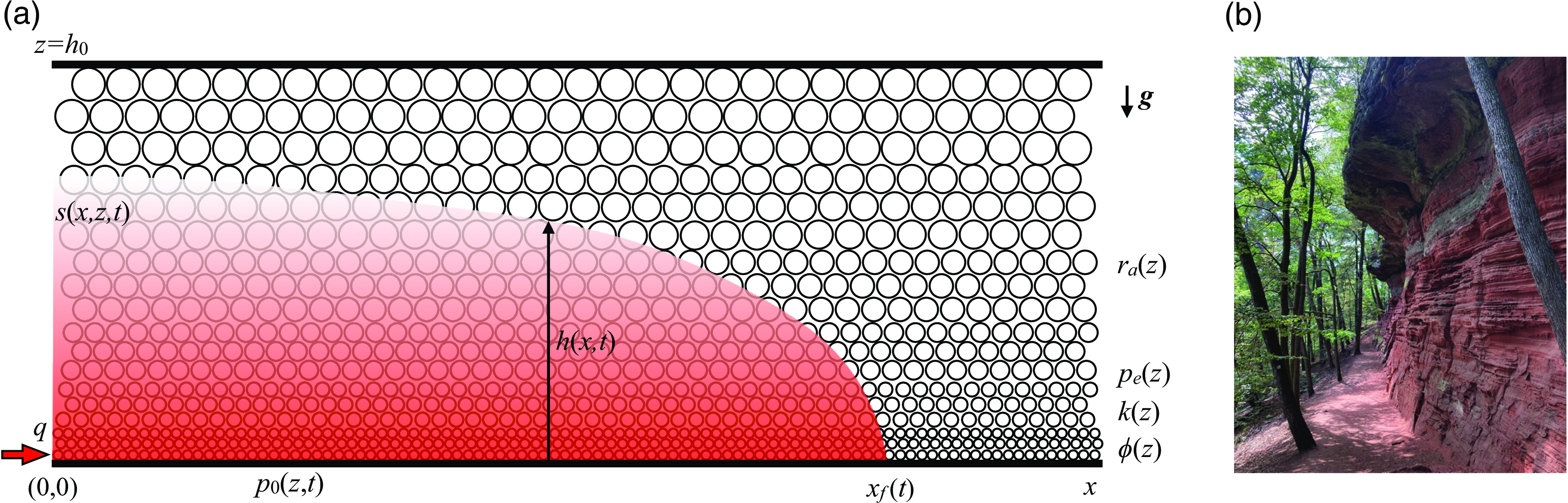
Figure 1. (a) Sketch of an unsaturated current invading into a porous layer with vertical heterogeneity and (b) a natural porous rock with vertical heterogeneity (Image Copyright: D. Geyer). $r_a(z)$
,
$r_a(z)$
, $\phi (z)$
and
$\phi (z)$
and $k(z)$
denote the pore radius, porosity and intrinsic permeability, respectively, and
$k(z)$
denote the pore radius, porosity and intrinsic permeability, respectively, and $p_e(z) \equiv \gamma \, \mbox{cos}\,\theta /r_a(z)$
denotes the capillary entry pressure. The injection rate, effective saturation and outer envelope of the invading fluid are denoted by
$p_e(z) \equiv \gamma \, \mbox{cos}\,\theta /r_a(z)$
denotes the capillary entry pressure. The injection rate, effective saturation and outer envelope of the invading fluid are denoted by $q$
,
$q$
, $s(x,z,t)$
, and
$s(x,z,t)$
, and $h(x,t)$
, respectively, and the location of the propagating front is denoted by
$h(x,t)$
, respectively, and the location of the propagating front is denoted by $x_f(t)$
. Also,
$x_f(t)$
. Also, $h_0$
represents the thickness of the porous layer.
$h_0$
represents the thickness of the porous layer.
Sedimentary porous rocks are often vertically heterogeneous: The porous rocks are typically layered with vertical variations of permeability by orders of magnitude between neighbouring layers, as shown in Figure 1. Within each layer, there exists also modest but (sometimes) non-negligible variations of permeability and porosity (Phillips Reference Phillips1991; Dullien Reference Dullien1992; Huppert & Woods Reference Huppert and Woods1995; Zheng et al. Reference Zheng, Soh, Huppert and Stone2013; Hinton & Woods Reference Hinton and Woods2018). For multi-phase flows, capillary pressure can also exhibit significant vertical variations in heterogeneous rocks, e.g. due to the variation of local curvature. Hence, the overall flow behaviours can be altered in both steady and unsteady situations, as can the overall performance in geophysical, environmental and industrial applications. For example, in petroleum and environmental engineering, it has long remained an important research topic to appropriately upscale single- and multi-phase flows in heterogeneous porous layers (Coats et al. Reference Coats, Dempsey and Henderson1971; Jackson et al. Reference Jackson, Agada, Reynolds and Krevor2018). The goal is typically to obtain appropriate relative permeability and capillary pressure curves, which can then be employed in transversely averaged flow and transport models at the reservoir scale (Zheng Reference Zheng2022).
In the context of unsteady flows, to our knowledge, the influence of heterogeneity has been investigated in detail for gravity currents (Huppert & Woods Reference Huppert and Woods1995; Zheng et al. Reference Zheng, Soh, Huppert and Stone2013; Hinton & Woods Reference Hinton and Woods2018), imbibition flows (Reyssat et al. Reference Reyssat, Courbin, Reyssat and Stone2008, Reference Reyssat, Sangne, Van Nierop and Stone2009), onset of hydrodynamic instabilities (Al-Housseiny et al. Reference Al-Housseiny, Tsai and Stone2012; Grenfell-Shaw et al. Reference Grenfell-Shaw, Hinton and Woods2021), and the transport of tracer and pollutant particles in porous rocks and filtering membranes (Dalwadi et al. Reference Dalwadi, Bruna and Griffiths2016; Hinton & Woods Reference Hinton and Woods2019). A common feature of these flows is that there exists typically a sharp fluid–fluid interface. The current work, nevertheless, looks further into the overlooked regime of unsteady unsaturated flows, as sketched in Figure 1. Key novel aspects of the current work include the following.
-
i. Compared with a previous study on a unified description of gravity current, interfacial and unsaturated flows in homogeneous porous layers (Zheng & Neufeld Reference Zheng and Neufeld2019), the current work further integrates the influence of vertical heterogeneity that could possibly appear in sedimentary porous rocks.
-
ii. Compared with a series of previous studies that investigated the time evolution of sharp fluid–fluid interfaces in vertically heterogeneous layers (Hinton & Woods Reference Hinton and Woods2018), we further resolve the saturation evolution of both the invading and the ambient fluids.
-
iii. Compared with a series of recent studies that model quasi-steady unsaturated flows in porous layers (Golding et al. Reference Golding, Neufeld, Hesse and Huppert2011; Zheng Reference Zheng2022), the current work keeps the unsteady term in the governing system and addresses the evolution dynamics of the saturation distribution and interface shape.
This paper is structured as follows. In §2, a theoretical model is first presented on the dynamics of gravity current, interfacial and unsaturated flows in vertically heterogeneous porous layers under the assumption of vertical gravitational-capillary equilibrium. This is followed by example calculations in the Cartesian configuration for some asymptotic and numerical insights. Then, in §3, potential implications of the model and solutions are discussed in the context of geological CO $_2$
sequestration, considering geophysical and operational parameters. This work is closed in §4 with a brief summary and final remarks on important model assumptions.
$_2$
sequestration, considering geophysical and operational parameters. This work is closed in §4 with a brief summary and final remarks on important model assumptions.
2. Theoretical model
We study one-dimensional predominantly horizontal flows in the Cartesian configuration, as illustrated in Figure 1. This set-up mimics some aspects of the displacement process generated from fluid injection through horizontal wells into a layer of sands, soil and rock formation. The injection rate $q$
is assumed to remain constant throughout the entire period of fluid injection. To highlight the influence of vertical heterogeneity, the variation of average pore size is assumed to follow the power-law form of
$q$
is assumed to remain constant throughout the entire period of fluid injection. To highlight the influence of vertical heterogeneity, the variation of average pore size is assumed to follow the power-law form of $r_a(z) \sim r_1 z^{\delta }$
, as is the intrinsic permeability
$r_a(z) \sim r_1 z^{\delta }$
, as is the intrinsic permeability $k(z) = k_0(r_1 z^\delta )^2$
and porosity
$k(z) = k_0(r_1 z^\delta )^2$
and porosity $\phi (z) = \phi _0 (r_1 z^\delta )^{2/n}$
. Such an assumption on heterogeneity in a model problem, including the correlation between porosity and intrinsic permeability, is consistent with a series of earlier reports (Huppert & Woods Reference Huppert and Woods1995; Reyssat et al. Reference Reyssat, Courbin, Reyssat and Stone2008; Zheng et al. Reference Zheng, Soh, Huppert and Stone2013; Ciriello et al. Reference Ciriello, Di Federico, Archetti and Longo2013; Zheng et al. Reference Zheng, Christov and Stone2014; Longo et al. Reference Longo, Ciriello, Chiapponi and Di Federico2015; Hinton & Woods Reference Hinton and Woods2018; Grenfell-Shaw et al. Reference Grenfell-Shaw, Hinton and Woods2021).
$\phi (z) = \phi _0 (r_1 z^\delta )^{2/n}$
. Such an assumption on heterogeneity in a model problem, including the correlation between porosity and intrinsic permeability, is consistent with a series of earlier reports (Huppert & Woods Reference Huppert and Woods1995; Reyssat et al. Reference Reyssat, Courbin, Reyssat and Stone2008; Zheng et al. Reference Zheng, Soh, Huppert and Stone2013; Ciriello et al. Reference Ciriello, Di Federico, Archetti and Longo2013; Zheng et al. Reference Zheng, Christov and Stone2014; Longo et al. Reference Longo, Ciriello, Chiapponi and Di Federico2015; Hinton & Woods Reference Hinton and Woods2018; Grenfell-Shaw et al. Reference Grenfell-Shaw, Hinton and Woods2021).
Meanwhile, we use the power-law form of relative permeability curves $k_{rn}(s) = k_{rn0}\,s^{\alpha }$
and
$k_{rn}(s) = k_{rn0}\,s^{\alpha }$
and $k_{rw}(s) = (1-s)^{\beta }$
(Brooks & Corey Reference Brooks and Corey1964), where we set
$k_{rw}(s) = (1-s)^{\beta }$
(Brooks & Corey Reference Brooks and Corey1964), where we set $\alpha =\beta =2$
. The capillary pressure curve is also assumed to follow the power-law form of
$\alpha =\beta =2$
. The capillary pressure curve is also assumed to follow the power-law form of $p_c(s) = \gamma \, \mbox{cos}\,\theta \,r_a^{-1} (1-s)^{-1/\Lambda }$
, with representative values of
$p_c(s) = \gamma \, \mbox{cos}\,\theta \,r_a^{-1} (1-s)^{-1/\Lambda }$
, with representative values of $\Lambda$
being
$\Lambda$
being $\Lambda = \{1/2,1,2,10\}$
. Note that
$\Lambda = \{1/2,1,2,10\}$
. Note that $\Lambda \to \infty$
suggests the existence of a sharp interface between the invading and the ambient fluids, which is also practically relevant. Note also that the capillary entry pressure follows
$\Lambda \to \infty$
suggests the existence of a sharp interface between the invading and the ambient fluids, which is also practically relevant. Note also that the capillary entry pressure follows $p_e(z) = \gamma \mbox{cos}\,\theta /(r_1 z^\delta )$
accordingly. The assumptions on the form of the
$p_e(z) = \gamma \mbox{cos}\,\theta /(r_1 z^\delta )$
accordingly. The assumptions on the form of the $k_{rn}(s)$
,
$k_{rn}(s)$
, $k_{rw}(s)$
and
$k_{rw}(s)$
and $p_c(s)$
curves are consistent with a series of earlier studies of unsaturated flows based on experimental observations of CO
$p_c(s)$
curves are consistent with a series of earlier studies of unsaturated flows based on experimental observations of CO $_2$
flooding in Ellerslie standstone (Golding et al. Reference Golding, Neufeld, Hesse and Huppert2011, Reference Golding, Huppert and Neufeld2013; Zheng & Neufeld Reference Zheng and Neufeld2019; Zheng Reference Zheng2022).
$_2$
flooding in Ellerslie standstone (Golding et al. Reference Golding, Neufeld, Hesse and Huppert2011, Reference Golding, Huppert and Neufeld2013; Zheng & Neufeld Reference Zheng and Neufeld2019; Zheng Reference Zheng2022).
A major advantage of using the power-law form of vertical heterogeneity is that it leads to an explicit expression for the saturation distribution $s(x,z,t)$
as a function of the profile shape
$s(x,z,t)$
as a function of the profile shape $h(x,t)$
. The remaining problem is then to solve for the interface shape evolution
$h(x,t)$
. The remaining problem is then to solve for the interface shape evolution $h(x,t)$
, which becomes somewhat standard in the context of gravity current flows (Huppert & Woods Reference Huppert and Woods1995; Pegler et al. Reference Pegler, Huppert and Neufeld2014; Zheng et al. Reference Zheng, Guo, Christov, Celia and Stone2015
a). Before we move on with detailed calculations, we note that the theory, in principle, applies to any form of vertical heterogeneity (though explicit solutions may not be available), providing that the assumption of vertical gravitational-capillary equilibrium continues to apply.
$h(x,t)$
, which becomes somewhat standard in the context of gravity current flows (Huppert & Woods Reference Huppert and Woods1995; Pegler et al. Reference Pegler, Huppert and Neufeld2014; Zheng et al. Reference Zheng, Guo, Christov, Celia and Stone2015
a). Before we move on with detailed calculations, we note that the theory, in principle, applies to any form of vertical heterogeneity (though explicit solutions may not be available), providing that the assumption of vertical gravitational-capillary equilibrium continues to apply.
2.1. Vertical gravitational-capillary equilibrium
When a current is long and thin, the incompressible flow condition ( $\nabla \cdot \mathbf{u} = 0$
) indicates that the vertical component of the Darcy velocity is negligible, compared with the horizontal component. This is a key feature of the propagation and displacement processes in this work, and is assumed to apply within the entire domain and throughout the entire time evolution. Effectively, the flow is predominantly one-dimensional, as the gravitational and capillary forces balance each other in the vertical direction (Golding et al. Reference Golding, Neufeld, Hesse and Huppert2011; Zheng & Neufeld Reference Zheng and Neufeld2019). Correspondingly, the pressure distribution within the invading and displaced fluids
$\nabla \cdot \mathbf{u} = 0$
) indicates that the vertical component of the Darcy velocity is negligible, compared with the horizontal component. This is a key feature of the propagation and displacement processes in this work, and is assumed to apply within the entire domain and throughout the entire time evolution. Effectively, the flow is predominantly one-dimensional, as the gravitational and capillary forces balance each other in the vertical direction (Golding et al. Reference Golding, Neufeld, Hesse and Huppert2011; Zheng & Neufeld Reference Zheng and Neufeld2019). Correspondingly, the pressure distribution within the invading and displaced fluids $p_n(x,z,t)$
and
$p_n(x,z,t)$
and $p_w(x,z,t)$
follows
$p_w(x,z,t)$
follows
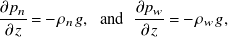 \begin{equation} \frac {\partial p_n}{\partial z} = -\rho _n g, \,\,\,\mbox{and}\,\,\, \frac {\partial p_w}{\partial z} = -\rho _w g, \end{equation}
which can be combined to provide a relationship between the capillary pressure $p_c(x,z,t) = p_n(x,z,t) - p_w(x,z,t)$
and buoyancy
$p_c(x,z,t) = p_n(x,z,t) - p_w(x,z,t)$
and buoyancy $\Delta \rho g$
as
$\Delta \rho g$
as
 \begin{equation} \frac {\partial p_c}{\partial z} = - \Delta \rho g. \end{equation}
This is an important result, which leads to an explicit expression between the saturation distribution $s(x,z,t)$
and the interface shape
$s(x,z,t)$
and the interface shape $h(x,t)$
as we show next.
$h(x,t)$
as we show next.
By integrating (2) along the $z$
direction, we next obtain
$z$
direction, we next obtain
 \begin{equation} p_c(s,z) - p_e(z) = -\Delta \rho g[z - h(x,t)]. \end{equation}
The boundary conditions employed upon integration are that $s[x,z=h(x,t),t]=0$
for the effective saturation and
$s[x,z=h(x,t),t]=0$
for the effective saturation and $p_c(s=0,z) \equiv p_e(z)$
for the capillary pressure along the outer envelope of the invading non-wetting fluid
$p_c(s=0,z) \equiv p_e(z)$
for the capillary pressure along the outer envelope of the invading non-wetting fluid $z=h(x,t)$
. Equation (3) can then be combined with
$z=h(x,t)$
. Equation (3) can then be combined with $p_c(s,z) = \frac {\gamma \mbox{cos}\,\theta }{r_a(z)} (1-s)^{-1/\Lambda }$
to provide an explicit expression for the effective saturation
$p_c(s,z) = \frac {\gamma \mbox{cos}\,\theta }{r_a(z)} (1-s)^{-1/\Lambda }$
to provide an explicit expression for the effective saturation $s(x,z,t)$
as
$s(x,z,t)$
as
 \begin{equation} s(x,z,t) = 1-\left (1-\frac {\Delta \rho g [z-h(x,t)]\, r_a(z)}{\gamma \mbox{cos}\,\theta }\right )^{-\Lambda }, \end{equation}
where we have assumed that the contact angle $\theta$
remains constant. Here,
$\theta$
remains constant. Here, $\Lambda$
is a fitting parameter, representing the pore-size distribution. Smaller
$\Lambda$
is a fitting parameter, representing the pore-size distribution. Smaller $\Lambda$
corresponds to a wider distribution of pore size, while
$\Lambda$
corresponds to a wider distribution of pore size, while $\Lambda \to +\infty$
indicates the limit of monodisperse pores with the same radius
$\Lambda \to +\infty$
indicates the limit of monodisperse pores with the same radius $r_a$
. Representative values for
$r_a$
. Representative values for $\Lambda$
that have been employed in previous studies are
$\Lambda$
that have been employed in previous studies are $\Lambda = \{1/2,1,2,10\}$
for the application of geological CO
$\Lambda = \{1/2,1,2,10\}$
for the application of geological CO $_2$
sequestration (Golding et al. Reference Golding, Neufeld, Hesse and Huppert2011, Reference Golding, Huppert and Neufeld2013; Zheng & Neufeld Reference Zheng and Neufeld2019; Zheng Reference Zheng2022). With (4), we know immediately that once
$_2$
sequestration (Golding et al. Reference Golding, Neufeld, Hesse and Huppert2011, Reference Golding, Huppert and Neufeld2013; Zheng & Neufeld Reference Zheng and Neufeld2019; Zheng Reference Zheng2022). With (4), we know immediately that once $h(x, t)$
is obtained, the saturation field
$h(x, t)$
is obtained, the saturation field $s(x,z,t)$
can be obtained conveniently.
$s(x,z,t)$
can be obtained conveniently.
In addition, under the assumption of vertical gravitational-capillary equilibrium, we can obtain the pressure distribution $p(x,z,t)$
by integrating (1) vertically:
$p(x,z,t)$
by integrating (1) vertically:
 \begin{align} p_n(x,z,t) = p_0(x,t) - \rho _n g z \quad \mbox{for}\,\,\, 0 \le z \le h(x,t),\quad \end{align}
 \begin{align} p_w(x,z,t) =p_0(x,t) - \rho _n g h - \rho _w g(z-h) - p_e(z) \quad \mbox{for}\ 0 \le z \le h_0,\quad \end{align}
where $p_0(x,t)$
is a reference pressure of the invading non-wetting fluid along the horizontal boundary (
$p_0(x,t)$
is a reference pressure of the invading non-wetting fluid along the horizontal boundary ( $z=0$
). The pressure gradient along the horizontal direction can then be calculated as
$z=0$
). The pressure gradient along the horizontal direction can then be calculated as
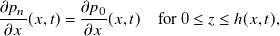 \begin{align} \frac {\partial p_n}{\partial x}(x,t) = \frac {\partial p_0}{\partial x}(x,t)\quad \mbox{for}\ 0 \le z \le h(x,t), \end{align}
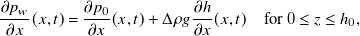 \begin{align} \frac {\partial p_w}{\partial x}(x,t) = \frac {\partial p_0}{\partial x}(x,t) + \Delta \rho g \frac {\partial h}{\partial x}(x,t) \quad \mbox{for}\ 0 \le z \le h_0, \end{align}
which can be substituted back into the generalised Darcy’s law to provide the horizontal velocities of each phase. It is of interest to note that neither $\partial p_n/\partial x$
nor
$\partial p_n/\partial x$
nor $\partial p_w/\partial x$
varies along the vertical direction
$\partial p_w/\partial x$
varies along the vertical direction $z$
, but in contrast, the pressure distribution
$z$
, but in contrast, the pressure distribution $p_n(x,z,t)$
and
$p_n(x,z,t)$
and $p_w(x,z,t)$
both exhibit vertical variations. This is a common feature of flow under vertical equilibrium.
$p_w(x,z,t)$
both exhibit vertical variations. This is a common feature of flow under vertical equilibrium.
2.2. Evolution equation
Following standard derivations (Zheng & Neufeld Reference Zheng and Neufeld2019), it is convenient to show that the time evolution of the interface shape $h(x,t)$
and saturation distribution
$h(x,t)$
and saturation distribution $s(x,z,t)$
is governed by the following set of differential and integral equations:
$s(x,z,t)$
is governed by the following set of differential and integral equations:
 \begin{align} (1-S_r) \frac {\partial I_s(h)}{\partial t} + q \frac {\partial }{\partial x} \left [\frac {M I_n(h)}{M I_n(h) + I_w(h)}\right ] - \frac {\Delta \rho g}{\mu _n} \frac {\partial }{\partial x} \left [\frac {I_n(h) I_w(h)}{M I_n(h) + I_w(h)} \frac {\partial h}{\partial x} \right ] = 0,\quad \quad \end{align}
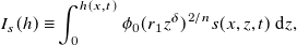 \begin{align} I_s(h) \equiv \int _0^{h(x,t)} \phi _0(r_1z^{\delta })^{2/n} s(x,z,t)\, \textrm {d}z, \quad \quad \end{align}
 \begin{align} I_n(h) \equiv \int _0^{h(x,t)}k_0(r_1z^{\delta })^2k_{rn}(s)\,\textrm {d}z,\quad I_w(h) \equiv \int _0^{h_0}k_0(r_1z^{\delta })^2k_{rw}(s)\,\textrm {d}z, \quad \quad \end{align}
and in particular, there is the explicit solution of $s(x,z,t)$
as a function of
$s(x,z,t)$
as a function of $h(x,t)$
:
$h(x,t)$
:
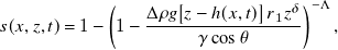 \begin{equation} s(x,z,t) = 1-\left (1-\frac {\Delta \rho g [z-h(x,t)]\, r_1 z^{\delta }}{\gamma \, \mbox{cos}\,\theta }\right )^{-\Lambda },\quad \quad \end{equation}
where we now substituted in the power-law form of $r_a(z) \sim r_1 z^{\delta }$
. As mentioned before, these results are based on the key assumption of vertical gravitational-capillary equilibrium for predominantly one-dimensional flows.
$r_a(z) \sim r_1 z^{\delta }$
. As mentioned before, these results are based on the key assumption of vertical gravitational-capillary equilibrium for predominantly one-dimensional flows.
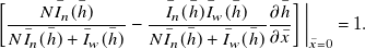
The initial-boundary value problem (7a) for $h(x,t)$
can be solved, providing appropriate initial and boundary conditions. When a fluid is injected at a constant rate
$h(x,t)$
can be solved, providing appropriate initial and boundary conditions. When a fluid is injected at a constant rate $q$
into a porous layer initially saturated with another immiscible fluid, the initial and boundary conditions are
$q$
into a porous layer initially saturated with another immiscible fluid, the initial and boundary conditions are
 \begin{align} h(x,0) = 0, \end{align}
 \begin{align} h(x_f(t),t) = 0, \end{align}
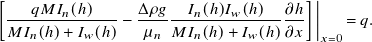 \begin{align} \left [\frac {q M I_n(h)}{M I_n(h) + I_w(h)} - \frac {\Delta \rho g}{\mu _n} \frac {I_n(h) I_w(h)}{M I_n(h) + I_w(h)} \frac {\partial h}{\partial x} \right ]\bigg |_{x=0} = q. \end{align}
Physically, (9a) represents an initial environment filled entirely with the ambient fluid within the entire domain. Equation (9b) is a frontal condition, with $x_f(t)$
denoting the location of a propagating front along the bottom boundary. Equation (9c) is a flux condition at the origin
$x_f(t)$
denoting the location of a propagating front along the bottom boundary. Equation (9c) is a flux condition at the origin $x=0$
and is obtained by integrating (7a) from
$x=0$
and is obtained by integrating (7a) from $x=0$
(location of fluid injection) towards
$x=0$
(location of fluid injection) towards $x=x_f(t)$
(location of the propagating front), applying the integral constraint of global mass conservation:
$x=x_f(t)$
(location of the propagating front), applying the integral constraint of global mass conservation:
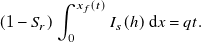 \begin{equation} (1-S_r)\int _0^{x_f(t)} I_s(h)\, \textrm {d}x = qt. \end{equation}
To obtain the flux boundary condition (9c), it is also assumed that there is no fluid entrainment at the location of the front at $x=x_f(t)$
, such that the local flux is zero at
$x=x_f(t)$
, such that the local flux is zero at $x=x_f(t)$
. Similar treatment has been employed previously in a series of fluid injection problems (Zheng et al. Reference Zheng, Guo, Christov, Celia and Stone2015
a). The problem formulation (7), (8) and (9), in principle, works for any functional form of
$x=x_f(t)$
. Similar treatment has been employed previously in a series of fluid injection problems (Zheng et al. Reference Zheng, Guo, Christov, Celia and Stone2015
a). The problem formulation (7), (8) and (9), in principle, works for any functional form of $k_{rn}(s)$
and
$k_{rn}(s)$
and $k_{rw}(s)$
, and here we impose
$k_{rw}(s)$
, and here we impose $k_{rn}(s) = k_{rn0}\,s^\alpha$
and
$k_{rn}(s) = k_{rn0}\,s^\alpha$
and $k_{rw}(s) = (1-s)^\beta$
for the example calculations, as summarised in Table 1.
$k_{rw}(s) = (1-s)^\beta$
for the example calculations, as summarised in Table 1.
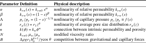
Table 1. Definition and physical meaning of the seven dimensionless parameters $\alpha$
,
$\alpha$
, $\beta$
,
$\beta$
, $\Lambda$
,
$\Lambda$
, $\delta$
,
$\delta$
, $n$
,
$n$
, $N$
and
$N$
and $B$
for predominantly one-dimensional flows in vertically heterogeneous porous layers
$B$
for predominantly one-dimensional flows in vertically heterogeneous porous layers
2.3. Non-dimensionalisation
We next non-dimensionalise (7), (8) and (9), and then discuss the asymptotic and numerical solutions and their physical interpretations. The dimensionless length, height, thickness and time are denoted by $\bar x \equiv x/x_c$
,
$\bar x \equiv x/x_c$
, $\bar z \equiv z/h_0$
,
$\bar z \equiv z/h_0$
, $\bar h \equiv h/h_0$
and
$\bar h \equiv h/h_0$
and $\bar t \equiv t/t_c$
, where the characteristic length and time scales are chosen as
$\bar t \equiv t/t_c$
, where the characteristic length and time scales are chosen as
 \begin{equation} x_c = \frac {\Delta \rho g k_0 k_{rn0} r_1^2 h_0^{2\delta +2}}{\mu _n q} \quad \mbox{and}\quad t_c = \frac {(1-S_r)\Delta \rho g k_0k_{rn0} \phi _0 r_1^{2/n+2} h_0^{2\delta /n+2\delta +3}}{\mu _n q^2}. \end{equation}
The scales $x_c$
and
$x_c$
and $t_c$
are chosen such that the unsteady, advective and diffusive terms balance each other in (7a) at
$t_c$
are chosen such that the unsteady, advective and diffusive terms balance each other in (7a) at $t \approx t_c$
for modest values of
$t \approx t_c$
for modest values of $M$
. The dimensionless frontal locations are
$M$
. The dimensionless frontal locations are $\bar x_f(\bar t) \equiv x_f(t)/x_c$
, and the dimensionless version of (7) and (8) becomes
$\bar x_f(\bar t) \equiv x_f(t)/x_c$
, and the dimensionless version of (7) and (8) becomes
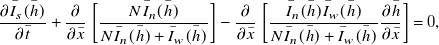 \begin{align} \frac {\partial \bar I_s(\bar h)}{\partial \bar t} + \frac {\partial }{\partial \bar x} \left [\frac {N \bar I_n(\bar h)}{N \bar I_n(\bar h) + \bar I_w(\bar h)}\right ] - \frac {\partial }{\partial \bar x} \left [\frac {\bar I_n(\bar h) \bar I_w(\bar h)}{N \bar I_n(\bar h) + \bar I_w(\bar h)} \frac {\partial \bar h}{\partial \bar x} \right ] = 0,\quad \end{align}
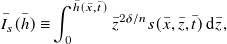 \begin{align} \bar I_s(\bar h) \equiv \int _0^{\bar h(\bar x, \bar t)} \bar z^{2\delta /n} s(\bar x,\bar z, \bar t)\, \textrm {d}\bar z, \quad \end{align}
 \begin{align} \bar I_n(\bar h) \equiv \int _0^{\bar h(\bar x, \bar t)}\bar z^{2\delta }s^{\alpha }\,\textrm {d}\bar z,\quad \bar I_w(\bar h) \equiv \int _0^{\bar h(\bar x, \bar t)}\bar z^{2\delta }(1-s)^\beta \,\textrm {d}\bar z+\frac {1-\bar h^{2\delta +1}}{2\delta +1} \quad \end{align}
and
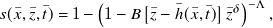 \begin{equation} s(\bar x, \bar z, \bar t) = 1-\left (1- B\, [\bar z - \bar h(\bar x, \bar t)]\, \bar z^{\delta }\right )^{-\Lambda }, \end{equation}
where the vertical integrals $\bar I_s(\bar h)$
,
$\bar I_s(\bar h)$
, $\bar I_n(\bar h)$
and
$\bar I_n(\bar h)$
and $\bar I_w (\bar h)$
are made dimensionless based on
$\bar I_w (\bar h)$
are made dimensionless based on
 \begin{equation} \bar I_s(\bar h) \equiv \frac {I_s(h)}{\phi _0 r_1^{2/n}h_0^{2\delta /n+1}},\quad \bar I_n(\bar h) \equiv \frac {I_n(h)}{k_0k_{rn0} r_1^2 h_0^{2\delta +1}} \quad\mbox{and}\quad \bar I_w (\bar h) \equiv \frac {I_w(h)}{k_0 r_1^2 h_0^{2\delta +1}}. \end{equation}
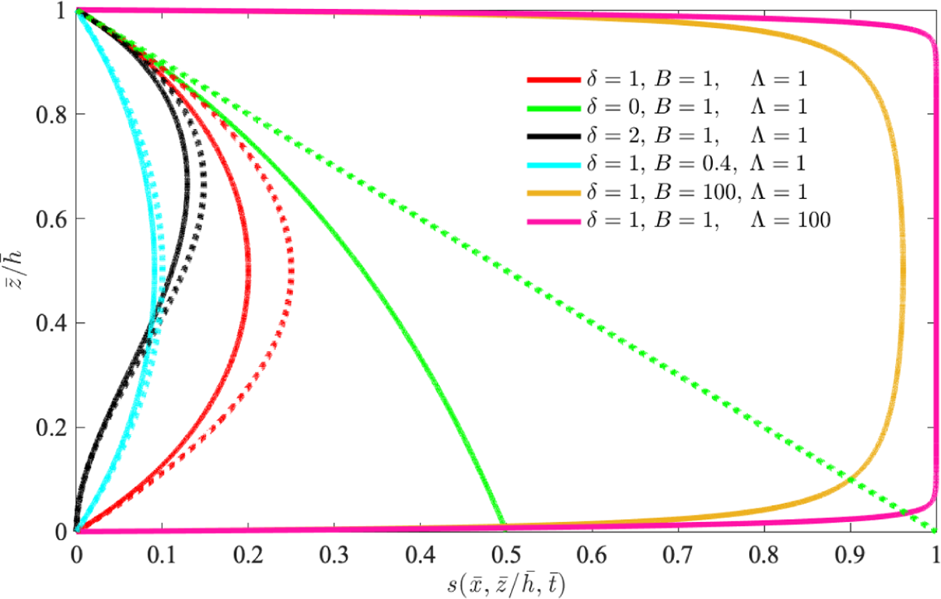
Figure 2. Representative solutions for the saturation field $s(\bar x, \bar z/\bar h, \bar t)$
along the vertical direction
$s(\bar x, \bar z/\bar h, \bar t)$
along the vertical direction $\bar z/\bar h(\bar x, \bar t)$
at any horizontal location
$\bar z/\bar h(\bar x, \bar t)$
at any horizontal location $\bar x$
at any time
$\bar x$
at any time $\bar t$
. The solid curves are based on (13), while the dashed curves are the asymptotes (17) that apply only when
$\bar t$
. The solid curves are based on (13), while the dashed curves are the asymptotes (17) that apply only when $B \ll 1$
for significantly unsaturated flows. The saturation field approaches the sharp-interface solution (35) when
$B \ll 1$
for significantly unsaturated flows. The saturation field approaches the sharp-interface solution (35) when $B \gg 1$
or when
$B \gg 1$
or when $\Lambda \gg 1$
.
$\Lambda \gg 1$
.
We have introduced two dimensionless parameters $N$
and
$N$
and $B$
in (12a) and (13), defined as
$B$
in (12a) and (13), defined as
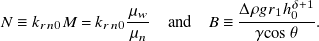 \begin{equation} N \equiv k_{rn0} M = k_{rn0} \frac {\mu _w}{\mu _n}\quad \mbox{and}\quad B \equiv \frac {\Delta \rho g r_1 h_0^{\delta +1}}{\gamma \mbox{cos}\,\theta }. \end{equation}
Physically, $N$
represents a ‘modified’ viscosity ratio, now including the influence of the end-point relative permeability
$N$
represents a ‘modified’ viscosity ratio, now including the influence of the end-point relative permeability $k_{rn0}$
of the invading fluid. This is also recognised by Zheng & Neufeld (Reference Zheng and Neufeld2019) for predominantly one-dimensional flows in an homogeneous porous layer. The Bond number
$k_{rn0}$
of the invading fluid. This is also recognised by Zheng & Neufeld (Reference Zheng and Neufeld2019) for predominantly one-dimensional flows in an homogeneous porous layer. The Bond number $B$
provides a measurement of the competition between the gravitational and capillary forces across the entire thickness of a vertically heterogeneous porous layer. Note also that
$B$
provides a measurement of the competition between the gravitational and capillary forces across the entire thickness of a vertically heterogeneous porous layer. Note also that $B$
reduces to
$B$
reduces to $1/H_e$
for Zheng & Neufeld (Reference Zheng and Neufeld2019) for flow in homogeneous layers, where
$1/H_e$
for Zheng & Neufeld (Reference Zheng and Neufeld2019) for flow in homogeneous layers, where $H_e$
is effectively a dimensionless capillary entry length. Similarly,
$H_e$
is effectively a dimensionless capillary entry length. Similarly, $1/B$
can also be understood as a dimensionless capillary entry length in a vertically heterogeneous layer. The solutions are under the influence of seven dimensionless parameters
$1/B$
can also be understood as a dimensionless capillary entry length in a vertically heterogeneous layer. The solutions are under the influence of seven dimensionless parameters $\alpha$
,
$\alpha$
, $\beta$
,
$\beta$
, $\Lambda$
,
$\Lambda$
, $\delta$
,
$\delta$
, $n$
,
$n$
, $N$
and
$N$
and $B$
, the definition and physical meaning of which are summarised in Table 1.
$B$
, the definition and physical meaning of which are summarised in Table 1.
Meanwhile, the initial and boundary conditions (9) can also be made dimensionless as
 \begin{align} \bar h(\bar x,0) = 0, \end{align}
 \begin{align} \bar h(\bar x_f(\bar t), \bar t) = 0, \end{align}
 \begin{align} \left [\frac {N \bar I_n(\bar h)}{N \bar I_n(\bar h) + \bar I_w(\bar h)} - \frac {\bar I_n(\bar h) \bar I_w(\bar h)}{N \bar I_n(\bar h) + \bar I_w(\bar h)} \frac {\partial \bar h}{\partial \bar x} \right ]\bigg |_{\bar x=0} = 1. \end{align}
We are now ready to explore solutions of the dimensionless system (12) subject to (16). In particular, (13) indicates that the saturation field $s(\bar x, \bar z, \bar t)$
is under the influence of three dimensionless control parameters:
$s(\bar x, \bar z, \bar t)$
is under the influence of three dimensionless control parameters: $\delta$
, a description of vertical heterogeneity;
$\delta$
, a description of vertical heterogeneity; $\Lambda$
, an indication of the pore size distribution; and
$\Lambda$
, an indication of the pore size distribution; and $B$
, a measurement of the competition between buoyancy and capillary forces. Typical solutions of
$B$
, a measurement of the competition between buoyancy and capillary forces. Typical solutions of $s(\bar x, \bar z, \bar t)$
are shown in Figure 2 for representative values of
$s(\bar x, \bar z, \bar t)$
are shown in Figure 2 for representative values of $\delta$
,
$\delta$
, $B$
and
$B$
and $\Lambda$
of practical relevance. We observe that
$\Lambda$
of practical relevance. We observe that $s(\bar x, \bar z, \bar t)$
is not monotonic along the
$s(\bar x, \bar z, \bar t)$
is not monotonic along the $z$
direction when
$z$
direction when $\delta \gt 0$
, which indicates there exists no flow of the invading fluid along
$\delta \gt 0$
, which indicates there exists no flow of the invading fluid along $z = 0$
and is consistent with the assumption that
$z = 0$
and is consistent with the assumption that $k = 0$
and
$k = 0$
and $\phi = 0$
along
$\phi = 0$
along $z=0$
.
$z=0$
.
2.4. Significantly unsaturated and sharp-interface flow regimes
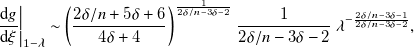
Analytical insights can be obtained in the significantly unsaturated and sharp-interface flow regimes, as we now discuss in §§ 2.4.1 and 2.4.2, respectively. Particular focus is placed on the unsaturated flow regime in the present work, since the key features in the sharp-interface flow regime have already been discussed (Huppert & Woods Reference Huppert and Woods1995; Hinton & Woods Reference Hinton and Woods2018). Due to the page limit for the maintext, we only show the early-time and late-time asymptotic behaviours in § 2.4.1, and in the supplementary material (SM) available at http://dx.doi.org/10.1017/flo.2025.13, we include also numerical solutions to demonstrate the time transition across time scales and how the flow approaches the early-time unconfined and late-time confined asymptotes in the corresponding asymptotic limits. The numerical scheme employed is also briefly described in the SM.
2.4.1. Significantly unsaturated flow regime
For modest values of $B$
, the fluid saturation
$B$
, the fluid saturation $s(\bar x, \bar z, \bar t)$
exhibits spatial variations due to the influence of the wetting and capillary forces. When
$s(\bar x, \bar z, \bar t)$
exhibits spatial variations due to the influence of the wetting and capillary forces. When $B \ll 1$
, named as the significantly unsaturated flow regime, (13) can be expanded as
$B \ll 1$
, named as the significantly unsaturated flow regime, (13) can be expanded as
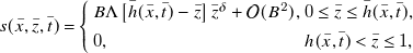 \begin{equation} s(\bar x, \bar z, \bar t) = \left \{\begin{array}{ll} B \Lambda \, [\bar h(\bar x, \bar t) - \bar z]\, \bar z^{\delta } + \mathcal{O}(B^2), & 0 \le \bar z \le \bar h(\bar x,\bar t), \\[4pt] 0, & h(\bar x,\bar t) \lt \bar z \le 1, \end{array} \right .\quad \quad \end{equation}
as a leading-order approximate for the saturation field. Equation (17) is plausible, since it allows analytical insights to understand the influence of vertical heterogeneity on unsaturated flows in porous layers. Based on (17), the rescaled solution $s(\bar x, \bar z, \bar t)/B\Lambda$
is only under the influence of
$s(\bar x, \bar z, \bar t)/B\Lambda$
is only under the influence of $\delta$
, the nonlinearity exponent for the pore size distribution
$\delta$
, the nonlinearity exponent for the pore size distribution $r_a(z) = r_1 z^\delta$
of the porous layer. Equation (17) is also included in Figure 2 as the dashed curves, which is to be compared with the original solution (13).
$r_a(z) = r_1 z^\delta$
of the porous layer. Equation (17) is also included in Figure 2 as the dashed curves, which is to be compared with the original solution (13).
To start, by substituting (17) back into (12b,c), we obtain approximate solutions for the vertical integrals $\bar I_s(\bar h)$
,
$\bar I_s(\bar h)$
, $\bar I_n(\bar h)$
and
$\bar I_n(\bar h)$
and $\bar I_w(\bar h)$
within the significantly unsaturated flow regime (
$\bar I_w(\bar h)$
within the significantly unsaturated flow regime ( $B \ll 1$
):
$B \ll 1$
):
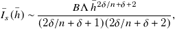 \begin{align} \bar I_s(\bar h) \sim \frac {B\Lambda \,\bar h^{2\delta /n+\delta +2}}{(2\delta /n+\delta +1)(2\delta /n+\delta + 2)}, \quad \end{align}
 \begin{align} \bar I_n(\bar h) \sim \frac {2B^2 \Lambda ^2 \,\bar h^{4\delta +3}}{(4\delta +1)(4\delta +2)(4\delta +3)},\quad \end{align}
 \begin{align} \bar I_w(\bar h) \sim \frac {1}{2\delta +1} - \frac {2B\Lambda \, \bar h^{3\delta +2}}{(3\delta +1)(3\delta +2)} + \frac {2B^2\Lambda ^2 \,\bar h^{4\delta +3}}{(4\delta +1)(4\delta +2)(4\delta +3)}, \quad \end{align}
where we have further imposed $\alpha =\beta =2$
for the relative permeability curves Golding et al. Reference Golding, Neufeld, Hesse and Huppert2011; Zheng & Neufeld Reference Zheng and Neufeld2019).
$\alpha =\beta =2$
for the relative permeability curves Golding et al. Reference Golding, Neufeld, Hesse and Huppert2011; Zheng & Neufeld Reference Zheng and Neufeld2019).
(i) Early-time asymptotic solutions $(\bar t \ll 1)$
At early times, defined by $\bar t \ll 1$
, the front of the invading fluid locates at
$\bar t \ll 1$
, the front of the invading fluid locates at $\bar x_f(\bar t) \ll 1$
and the thickness of the invading fluid is also small
$\bar x_f(\bar t) \ll 1$
and the thickness of the invading fluid is also small $\bar h(\bar x, \bar t) \ll 1$
such that
$\bar h(\bar x, \bar t) \ll 1$
such that $\bar I_n(\bar h) \ll \bar I_w(\bar h)$
. In this case, the nonlinear diffusive term is much greater than the advective term, and the governing system (12a) further reduces to
$\bar I_n(\bar h) \ll \bar I_w(\bar h)$
. In this case, the nonlinear diffusive term is much greater than the advective term, and the governing system (12a) further reduces to
 \begin{equation} \frac {\partial \bar I_s(\bar h)}{\partial \bar t} - \frac {\partial }{\partial \bar x} \left [\bar I_n(\bar h) \frac {\partial \bar h}{\partial \bar x} \right ] = 0.\quad \end{equation}
Then, by substituting (18) into (19), we arrive at a nonlinear diffusion equation for the time evolution of the interface shape $\bar h(\bar x, \bar t)$
that is very similar to those obtained by Boussinesq (Reference Boussinesq1904) and Huppert (Reference Huppert1982):
$\bar h(\bar x, \bar t)$
that is very similar to those obtained by Boussinesq (Reference Boussinesq1904) and Huppert (Reference Huppert1982):
 \begin{equation} \frac {\partial \bar h^{2\delta /n+\delta +2}}{\partial \bar t} - A_1\,\frac {\partial }{\partial \bar x} \left (\bar h^{4\delta +3} \frac {\partial \bar h}{\partial \bar x} \right ) = 0,\quad\mbox{where}\,\,\,A_1 \equiv \frac {2B\Lambda (2\delta /n+\delta +1)(2\delta /n+\delta +2)}{(4\delta +1)(4\delta +2)(4\delta +3)}. \end{equation}
The partial differential equation (PDE) (20) can be solved, providing a frontal condition $\bar h(\bar x_f(\bar t), \bar t) = 0$
and an integral condition for the fluid volume:
$\bar h(\bar x_f(\bar t), \bar t) = 0$
and an integral condition for the fluid volume:
 \begin{equation} \int _0^{\bar x_f(\bar t)}\, A_2\,\bar h^{2\delta /n+\delta +2}\,\textrm {d}\bar x = \bar t,\,\,\,\mbox{where}\,\,\, A_2 \equiv \frac {B\Lambda }{(2\delta /n+\delta +1)(2\delta /n+\delta +2)}. \end{equation}
Nevertheless, it is important to note that, physically, (20) and (21) describe the invasion of a capillary film into a porous layer, rather than the propagation of a viscous gravity current (Huppert Reference Huppert1982). This is more clearly seen in the dimensional form of (20), which depends explicitly on surface tension $\gamma$
rather than buoyancy
$\gamma$
rather than buoyancy $\Delta \rho g$
. The interface shape
$\Delta \rho g$
. The interface shape $\bar h(\bar x, \bar t)$
is now under the influence of three dimensionless parameters:
$\bar h(\bar x, \bar t)$
is now under the influence of three dimensionless parameters: $\delta$
and
$\delta$
and $n$
, which characterise the intrinsic properties of the porous layer, and
$n$
, which characterise the intrinsic properties of the porous layer, and $B\Lambda$
, an indication of the competition between buoyancy and capillary forces in an heterogeneous environment. Also, there is no role of the modified viscosity ratio
$B\Lambda$
, an indication of the competition between buoyancy and capillary forces in an heterogeneous environment. Also, there is no role of the modified viscosity ratio $N$
, since flow of the invading fluid is unconfined and flow of the displaced fluid is negligible. Once
$N$
, since flow of the invading fluid is unconfined and flow of the displaced fluid is negligible. Once $\bar h(\bar x, \bar t)$
is obtained from solving (20) and (21), the saturation field
$\bar h(\bar x, \bar t)$
is obtained from solving (20) and (21), the saturation field $s(\bar x, \bar z, \bar t)$
can then be obtained from (17).
$s(\bar x, \bar z, \bar t)$
can then be obtained from (17).
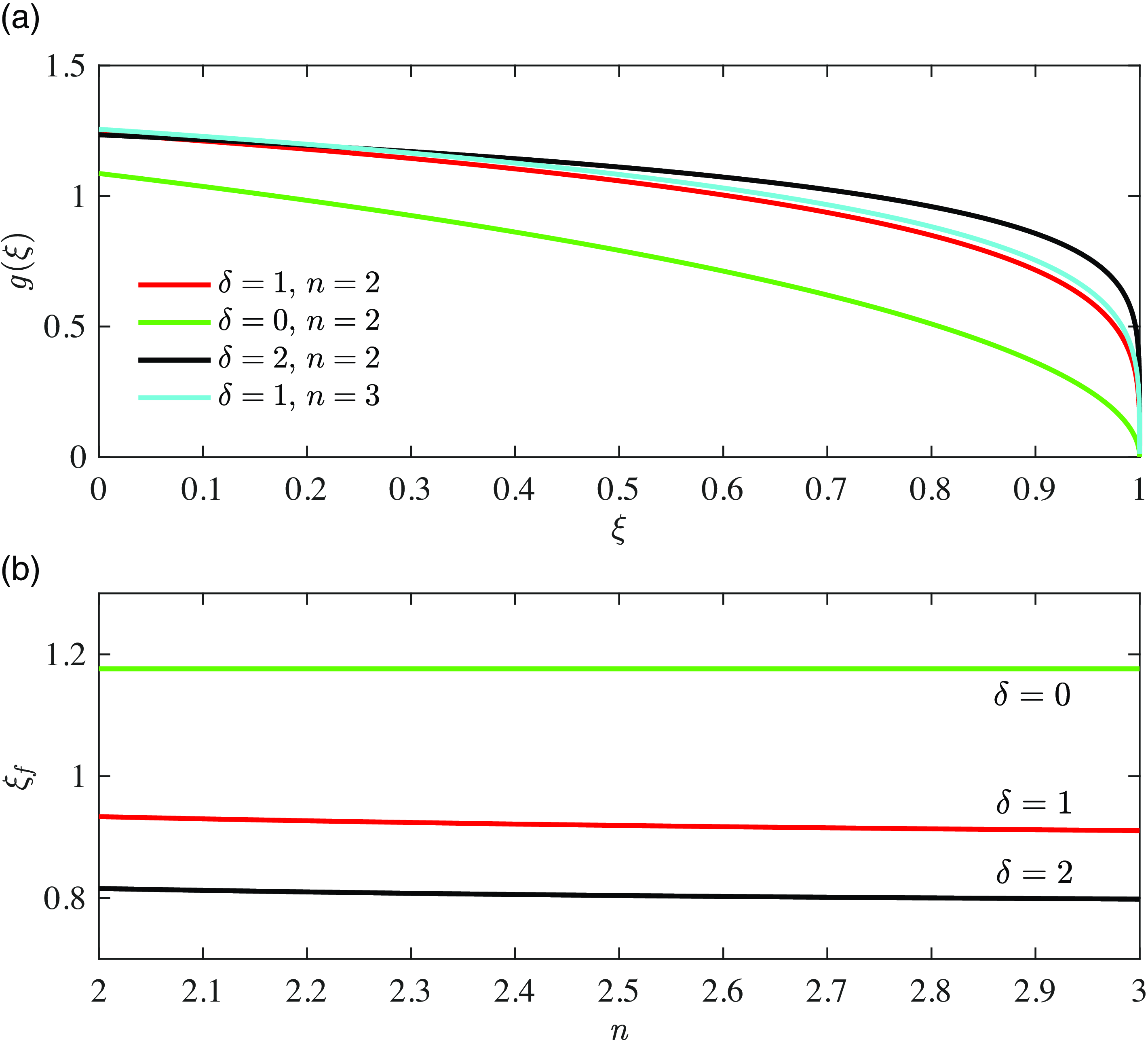
Figure 3. Influence of heterogeneity on (a) the early-time self-similar solution $g(\xi )$
and (b) the frontal location
$g(\xi )$
and (b) the frontal location $\xi _f$
for selected values of
$\xi _f$
for selected values of $\delta$
and
$\delta$
and $n$
from solving (23). The case of
$n$
from solving (23). The case of $\delta =0$
is also plotted as a comparison, which represents unconfined unsaturated flow in a homogeneous porous layer.
$\delta =0$
is also plotted as a comparison, which represents unconfined unsaturated flow in a homogeneous porous layer.
Self-similar solutions can also be explored for the time evolution of the interface shape $\bar h(\bar x, \bar t)$
, as is suggested by the form of (20) and (21). We can start by defining a similarity transform as
$\bar h(\bar x, \bar t)$
, as is suggested by the form of (20) and (21). We can start by defining a similarity transform as
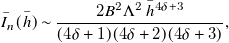
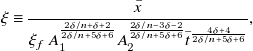 \begin{align} \xi \equiv \frac {\bar x}{\xi _f \,A_1^{\frac {2\delta /n+\delta +2}{2\delta /n+5\delta +6}}A_2^{\frac {2\delta /n-3\delta -2}{2\delta /n+5\delta +6}} \bar t^{\frac {4\delta + 4}{2\delta /n + 5\delta + 6}}}, \end{align}
 \begin{align} \bar h(\bar x, \bar t) = \xi _f^{-\frac {2}{2\delta /n-3\delta -2}}\,\left (A_1A_2^2\right )^{\frac {-1}{2\delta /n+5\delta +6}} \bar t^{\frac {1}{2\delta /n+5\delta +6}}\, g(\xi ), \end{align}
where $\xi \in [0,1]$
, with the propagating front locating at
$\xi \in [0,1]$
, with the propagating front locating at $\bar x_f(\bar t) = \xi _f A_1^{\frac {2\delta /n+\delta +2}{2\delta /n+5\delta +6}}A_2^{\frac {2\delta /n-3\delta -2}{2\delta /n+5\delta +6}}\bar t^{\frac {4\delta + 4}{2\delta /n + 5\delta + 6}}$
as time progresses. Under transform (22a,b), (20) and (21) are transformed into
$\bar x_f(\bar t) = \xi _f A_1^{\frac {2\delta /n+\delta +2}{2\delta /n+5\delta +6}}A_2^{\frac {2\delta /n-3\delta -2}{2\delta /n+5\delta +6}}\bar t^{\frac {4\delta + 4}{2\delta /n + 5\delta + 6}}$
as time progresses. Under transform (22a,b), (20) and (21) are transformed into
 \begin{align} \frac {2\delta /n+\delta +2}{2\delta /n+5\delta +6} g^{2\delta /n+\delta +2} - \frac {4\delta +4}{2\delta /n+5\delta +6}\xi \frac {\textrm {d}g^{2\delta /n+\delta +2}}{\textrm {d}\xi } - \frac {\textrm {d}}{\textrm {d}\xi }\left (g^{4\delta +3}\frac {\textrm {d} g}{\textrm {d}\xi }\right ) = 0,\quad \quad \end{align}
 \begin{align} \xi _f = \left (\int _0^1 g^{2\delta /n+\delta +2}\,\textrm {d}\xi \right )^{\frac {2\delta /n-3\delta -2}{2\delta /n+5\delta +6}},\quad \quad \end{align}
for the self-similar interface shape $g(\xi )$
and frontal location
$g(\xi )$
and frontal location $\xi _f$
. The above transform and descriptions from (20) to (23) are analogous exactly to those that describe the propagation of viscous gravity currents (Huppert Reference Huppert1982). We also note that, while the interface shape
$\xi _f$
. The above transform and descriptions from (20) to (23) are analogous exactly to those that describe the propagation of viscous gravity currents (Huppert Reference Huppert1982). We also note that, while the interface shape $\bar h(\bar x, \bar t)$
and frontal location
$\bar h(\bar x, \bar t)$
and frontal location $\bar x_f(\bar t)$
depend on
$\bar x_f(\bar t)$
depend on $B\Lambda$
, a measurement of the wetting and capillary effects, the self-similar shape
$B\Lambda$
, a measurement of the wetting and capillary effects, the self-similar shape $g(\xi )$
and prefactor
$g(\xi )$
and prefactor $\xi _f$
rely only on
$\xi _f$
rely only on $\delta$
and
$\delta$
and $n$
that describe the intrinsic properties of a vertical heterogeneity.
$n$
that describe the intrinsic properties of a vertical heterogeneity.
The ordinary differential equation (ODE) (23a
) can be solved numerically from $\xi =1-\lambda$
towards
$\xi =1-\lambda$
towards $\xi =0^+$
with
$\xi =0^+$
with $\lambda \ll 1$
. The boundary conditions at
$\lambda \ll 1$
. The boundary conditions at $\xi =1-\lambda$
are
$\xi =1-\lambda$
are
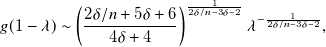 \begin{align} g(1-\lambda ) \sim \left (\frac {2\delta /n+5\delta +6}{4\delta +4}\right )^{\frac {1}{2\delta /n-3\delta -2}} \lambda ^{-\frac {1}{2\delta /n-3\delta -2}}, \end{align}
 \begin{align} \frac {\textrm {d}g}{\textrm {d}\xi }\bigg |_{1-\lambda } \sim \left (\frac {2\delta /n+5\delta +6}{4\delta +4}\right )^{\frac {1}{2\delta /n-3\delta -2}}\frac {1}{2\delta /n-3\delta -2}\, \lambda ^{-\frac {2\delta /n-3\delta -1}{2\delta /n-3\delta -2}}, \end{align}
as obtained from a local analysis of (23a
) that $g \sim [(2\delta /n+5\delta +6)/(4\delta +4)]^{1/(2\delta /n-3\delta -2)}(1-\xi )^{-1/(2\delta /n-3\delta -2)}$
as
$g \sim [(2\delta /n+5\delta +6)/(4\delta +4)]^{1/(2\delta /n-3\delta -2)}(1-\xi )^{-1/(2\delta /n-3\delta -2)}$
as $\xi \to 1^-$
. Once
$\xi \to 1^-$
. Once $g(\xi )$
is known, the prefactor
$g(\xi )$
is known, the prefactor $\xi _f$
can also be calculated from (23b
), and the dependence on
$\xi _f$
can also be calculated from (23b
), and the dependence on $\delta$
and
$\delta$
and $n$
can also be obtained. Typical results are shown in Figure 3a for the interface shape
$n$
can also be obtained. Typical results are shown in Figure 3a for the interface shape $g(\xi )$
, employing Matlab subroutine ODE45 (or ODE15s) setting
$g(\xi )$
, employing Matlab subroutine ODE45 (or ODE15s) setting $\lambda =10^{-8}$
. The prefactor
$\lambda =10^{-8}$
. The prefactor $\xi _f$
for the frontal location is also shown in Figure 3b for selected values of
$\xi _f$
for the frontal location is also shown in Figure 3b for selected values of $\delta$
and
$\delta$
and $n$
. It is found that the dependence of
$n$
. It is found that the dependence of $\xi _f$
on
$\xi _f$
on $n$
is rather weak. The saturation distribution
$n$
is rather weak. The saturation distribution $s(\bar \xi , \bar z, \bar t)$
, in addition, is shown in Figure 4, based on (17), where we imposed
$s(\bar \xi , \bar z, \bar t)$
, in addition, is shown in Figure 4, based on (17), where we imposed $\{\delta , n, B\Lambda \}= \{1, 2, 1/10\}$
as an example.
$\{\delta , n, B\Lambda \}= \{1, 2, 1/10\}$
as an example.
It is also of interest to provide a self-consistence check on the time scale for the condition of $\bar h \ll 1$
to apply. Based on (22b
), we obtain that
$\bar h \ll 1$
to apply. Based on (22b
), we obtain that $\bar h \approx (\bar t/A_1A_2^2)^{1/(2\delta /n+5\delta +6)}$
, which provides a time scale of
$\bar h \approx (\bar t/A_1A_2^2)^{1/(2\delta /n+5\delta +6)}$
, which provides a time scale of $\bar t_{c1} \approx A_1A_2^2$
for the interface to attach at both the top and bottom boundaries, i.e.
$\bar t_{c1} \approx A_1A_2^2$
for the interface to attach at both the top and bottom boundaries, i.e. $\bar h(0,\bar t_{c1}) \approx 1$
. In other words, it is required that
$\bar h(0,\bar t_{c1}) \approx 1$
. In other words, it is required that $\bar t \ll \bar t_{c1}$
for the early-time self-similar solution to apply. It is also suggested that the transition time scale
$\bar t \ll \bar t_{c1}$
for the early-time self-similar solution to apply. It is also suggested that the transition time scale $\bar t_{c1} \propto (B\Lambda )^3$
, which can be significantly impacted by the wetting and capillary effects. In addition,
$\bar t_{c1} \propto (B\Lambda )^3$
, which can be significantly impacted by the wetting and capillary effects. In addition, $\bar t_{c1} \propto 1/(4\delta +1)(4\delta +2)(4\delta +3)(2\delta /n+\delta +1)(2\delta /n+\delta +2)$
, so it is also under the influence of vertical heterogeneity.
$\bar t_{c1} \propto 1/(4\delta +1)(4\delta +2)(4\delta +3)(2\delta /n+\delta +1)(2\delta /n+\delta +2)$
, so it is also under the influence of vertical heterogeneity.
Figure 4. Time evolution of the profile shape $\bar h(\bar x, \bar t)$
based on the early- and late-time self-similar solutions (23) and (29) and the saturation distribution
$\bar h(\bar x, \bar t)$
based on the early- and late-time self-similar solutions (23) and (29) and the saturation distribution $s(\bar x, \bar z, \bar t)$
based on (17) in the significantly unsaturated flow regime (
$s(\bar x, \bar z, \bar t)$
based on (17) in the significantly unsaturated flow regime ( $B \ll 1$
).
$B \ll 1$
).
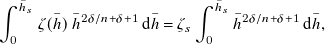
 $\bar h(\bar x, \bar t)$
evolves from a capillary film shape into either a compound-wave shape (
$\bar h(\bar x, \bar t)$
evolves from a capillary film shape into either a compound-wave shape ( $N \gt N_c$
) or a shock shape (
$N \gt N_c$
) or a shock shape ( $N \le N_c$
), depending on the modified viscosity ratio
$N \le N_c$
), depending on the modified viscosity ratio $N \equiv k_{rn0}\,\mu _d/\mu _i$
. We have imposed
$N \equiv k_{rn0}\,\mu _d/\mu _i$
. We have imposed $\delta =1$
,
$\delta =1$
, $n=2$
and
$n=2$
and $B\Lambda = 1/10$
in this example calculation.
$B\Lambda = 1/10$
in this example calculation.
(ii) Late-time asymptotic solutions $(\bar t \gg 1)$
At late times, defined by $\bar t \gg 1$
, we expect the length of the current
$\bar t \gg 1$
, we expect the length of the current $\bar x_f(\bar t) \gg 1$
, as it continues to elongate. Eventually, the contribution of the diffusive term (
$\bar x_f(\bar t) \gg 1$
, as it continues to elongate. Eventually, the contribution of the diffusive term ( $\propto \bar x_f^{-2}$
) becomes much smaller compared with the advective term (
$\propto \bar x_f^{-2}$
) becomes much smaller compared with the advective term ( $\propto \bar x_f^{-1}$
) in PDE (12a), except possibly in a narrow boundary layer near the propagating front
$\propto \bar x_f^{-1}$
) in PDE (12a), except possibly in a narrow boundary layer near the propagating front $\bar x_f(\bar t)$
, where singular perturbation effects become important. In the present work, we neglect such a frontal region and explore the late-time asymptotic behaviours of
$\bar x_f(\bar t)$
, where singular perturbation effects become important. In the present work, we neglect such a frontal region and explore the late-time asymptotic behaviours of $\bar h(\bar x, \bar t)$
simply by studying the advective equation
$\bar h(\bar x, \bar t)$
simply by studying the advective equation
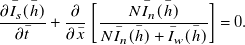 \begin{equation} \frac {\partial \bar I_s(\bar h)}{\partial \bar t} + \frac {\partial }{\partial \bar x} \left [\frac {N \bar I_n(\bar h)}{N \bar I_n(\bar h) + \bar I_w(\bar h)}\right ] = 0.\quad \end{equation}
Self-similar solutions can also be explored, now by defining a similarity variable as $\zeta \equiv \bar x/\bar t$
, and hence
$\zeta \equiv \bar x/\bar t$
, and hence $\bar h (\bar x, \bar t) = \bar h (\zeta )$
. The PDE (25) is then transformed into
$\bar h (\bar x, \bar t) = \bar h (\zeta )$
. The PDE (25) is then transformed into
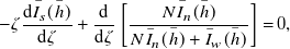 \begin{equation} -\zeta \frac {\textrm {d} \bar I_s(\bar h)}{\textrm {d} \zeta } + \frac {\textrm {d}}{\textrm {d}\zeta } \left [\frac {N \bar I_n(\bar h)}{N \bar I_n(\bar h) + \bar I_w(\bar h)}\right ] = 0, \end{equation}
the solution of which is under the influence of all seven dimensionless control parameters $\alpha$
,
$\alpha$
, $\beta$
,
$\beta$
, $\Lambda$
,
$\Lambda$
, $\delta$
,
$\delta$
, $n$
,
$n$
, $N$
and
$N$
and $B$
. Neglecting the solution branch of
$B$
. Neglecting the solution branch of $\textrm {d}\bar h/\textrm {d} \zeta = 0$
, ODE (26) can be further rearranged to provide an algebraic equation for the self-similar solution
$\textrm {d}\bar h/\textrm {d} \zeta = 0$
, ODE (26) can be further rearranged to provide an algebraic equation for the self-similar solution $\bar h(\zeta )$
as
$\bar h(\zeta )$
as
 \begin{equation} \zeta = \frac {\textrm {d}}{\textrm {d}\bar h} \left [\frac {N \bar I_n(\bar h)}{N \bar I_n(\bar h) + \bar I_w(\bar h)}\right ] \bigg / \frac {\textrm {d} \bar I_s(\bar h)}{\textrm {d} \bar h}. \end{equation}
Once $\bar h(\zeta )$
is known, the saturation field
$\bar h(\zeta )$
is known, the saturation field $s(\zeta , \bar z)$
can also be calculated based on (17).
$s(\zeta , \bar z)$
can also be calculated based on (17).
Again, we look into the significantly unsaturated flow regime ( $B\ll 1$
), when the integrals
$B\ll 1$
), when the integrals $\bar I_s(\bar h)$
,
$\bar I_s(\bar h)$
, $\bar I_n(\bar h)$
and
$\bar I_n(\bar h)$
and $\bar I_w(\bar h)$
can be approximated by (18). Then, by substituting (18) into (25), we obtain
$\bar I_w(\bar h)$
can be approximated by (18). Then, by substituting (18) into (25), we obtain
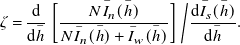
 \begin{align} \frac {\partial \bar h^{2\delta /n+\delta +2}}{\partial \bar t} + \frac {\partial }{\partial \bar x}\left [\frac {C_1\,N\bar h^{4\delta +3}}{1-C_2\,\bar h^{3\delta +2}+C_3\,(N+1)\bar h^{4\delta +3}}\right ] = 0, \end{align}
 \begin{align} \mbox{with}\,\,\,C_1 \equiv \frac {2B\Lambda (2\delta +1)(2\delta /n+\delta +1)(2\delta /n+\delta +2)}{(4\delta +1)(4\delta +2)(4\delta +3)}, \end{align}
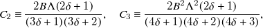 \begin{align} C_2 \equiv \frac {2B\Lambda (2\delta +1)}{(3\delta +1)(3\delta +2)},\quad C_3 \equiv \frac {2B^2\Lambda ^2(2\delta +1)}{(4\delta +1)(4\delta +2)(4\delta +3)}, \end{align}
for the time evolution of $\bar h(\bar x, \bar t)$
, or
$\bar h(\bar x, \bar t)$
, or
 \begin{align} \zeta &= \frac {1}{(2\delta /n+\delta +2)\,\bar h^{2\delta /n+\delta +1} }\frac {\textrm {d}}{\textrm {d} \bar h}\left [\frac {C_1\,N\bar h^{4\delta +3}}{1-C_2\,\bar h^{3\delta +2}+C_3\,(N+1)\bar h^{4\delta +3}}\right ] \end{align}
 \begin{align} &= \frac {(4\delta +3) C_1 N \bar h^{-2\delta /n+3\delta +1} -(\delta +1)C_1C_2 N \bar h^{-2\delta /n+6\delta +3}}{(2\delta /n+\delta +2)[1 - C_2\bar h^{3\delta +2} + C_3(N+1) \bar h^{4\delta +3}]^2}, \end{align}
for a self-similar solution $\bar h(\zeta )$
at late times. Solutions to (28) or (29) are under the influence of four dimensionless parameters:
$\bar h(\zeta )$
at late times. Solutions to (28) or (29) are under the influence of four dimensionless parameters: $\delta$
,
$\delta$
, $n$
,
$n$
, $ N$
and
$ N$
and $B\Lambda$
, and once again,
$B\Lambda$
, and once again, $B$
and
$B$
and $\Lambda$
function together as a group
$\Lambda$
function together as a group $B\Lambda$
.
$B\Lambda$
.
To explore the solution structure of the advective system, we first comment on the height of the current $\bar h_i$
at the inlet
$\bar h_i$
at the inlet $\bar x = 0$
. By substituting (18) into (16c) and neglecting the diffusive term that is
$\bar x = 0$
. By substituting (18) into (16c) and neglecting the diffusive term that is $\propto \partial \bar h/\partial \bar x$
in (16c), it is shown that the inlet height
$\propto \partial \bar h/\partial \bar x$
in (16c), it is shown that the inlet height $\bar h_i$
must satisfy
$\bar h_i$
must satisfy $\bar I_w(\bar h_i) = 0$
, i.e.
$\bar I_w(\bar h_i) = 0$
, i.e.
 \begin{equation} \frac {1}{2\delta +1}-\frac {2B\Lambda \bar h_i^{3\delta +2}}{(3\delta +1)(3\delta +2)}+\frac {2B^2\Lambda ^2 \bar h_i^{4\delta +3}}{(4\delta +1)(4\delta +2)(4\delta +3)} = 0, \end{equation}
in the significantly unsaturated regime ( $B\ll 1$
). However, when
$B\ll 1$
). However, when $\delta \gt 0$
and
$\delta \gt 0$
and $B\Lambda \gt 0$
, there is no solution for (30) for
$B\Lambda \gt 0$
, there is no solution for (30) for $\bar h_i \in (0,1)$
. Therefore, the inlet height must always be
$\bar h_i \in (0,1)$
. Therefore, the inlet height must always be $\bar h_i = 1$
at late times, with
$\bar h_i = 1$
at late times, with $|\partial \bar h/\partial \bar x| (0, t) \gt 0$
to satisfy boundary condition (16c). This conclusion is also consistent with the numerical observations when we solve PDE (12a).
$|\partial \bar h/\partial \bar x| (0, t) \gt 0$
to satisfy boundary condition (16c). This conclusion is also consistent with the numerical observations when we solve PDE (12a).
Figure 5. Regime diagram for significantly unsaturated flows in vertically heterogeneous porous layers when the modified viscosity ratio $N$
varies, imposing
$N$
varies, imposing $\{\delta , n, B\Lambda \} = \{1,2,1/10\}$
as an example. The height
$\{\delta , n, B\Lambda \} = \{1,2,1/10\}$
as an example. The height $\bar h_s$
and location
$\bar h_s$
and location $\zeta _s$
for the inserted shock front are also shown.
$\zeta _s$
for the inserted shock front are also shown.
Correspondingly, when $\delta \gt 0$
, (29) leads to two solution branches in the significantly unsaturated flow regime (
$\delta \gt 0$
, (29) leads to two solution branches in the significantly unsaturated flow regime ( $B\ll 1$
): (i) compound-wave solutions for sufficiently large viscosity contrast
$B\ll 1$
): (i) compound-wave solutions for sufficiently large viscosity contrast $N \gt N_c$
; and (ii) shock solutions for
$N \gt N_c$
; and (ii) shock solutions for $N \le N_c$
, where
$N \le N_c$
, where $N_c$
is a critical viscosity ratio that depends on the value of
$N_c$
is a critical viscosity ratio that depends on the value of $\delta$
,
$\delta$
, $n$
and
$n$
and $B\Lambda$
. To obtain the compound-wave solutions, a shock front of height
$B\Lambda$
. To obtain the compound-wave solutions, a shock front of height $\bar h_s \in (0,1)$
is inserted at an appropriate location
$\bar h_s \in (0,1)$
is inserted at an appropriate location $\zeta _s$
to ensure the conservation of total fluid volume. Based on (18a), the total volume of the invading fluid
$\zeta _s$
to ensure the conservation of total fluid volume. Based on (18a), the total volume of the invading fluid $\textrm {d}\bar I_s(\bar h)$
within a thin layer
$\textrm {d}\bar I_s(\bar h)$
within a thin layer $[\bar h, \bar h+\textrm {d}\bar h]$
is given by
$[\bar h, \bar h+\textrm {d}\bar h]$
is given by
 \begin{equation} \textrm {d}\bar I_s(\bar h) = \frac {B\Lambda \, \bar h^{2\delta /n+\delta +1}}{(2\delta /n+\delta +1)} \textrm {d}\bar h, \end{equation}
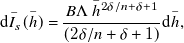
which leads to
 \begin{equation} \int _0^{\bar h_s} \zeta (\bar h)\, \bar h^{2\delta /n+\delta +1}\,\textrm {d}\bar h = \zeta _s \int _0^{\bar h_s} \bar h^{2\delta /n+\delta +1}\,\textrm {d}\bar h, \end{equation}
for the height $\bar h_s$
and location
$\bar h_s$
and location $\zeta _s$
of the inserted shock front. Combining (29) and (32), we can calculate
$\zeta _s$
of the inserted shock front. Combining (29) and (32), we can calculate $(\zeta _s, \bar h_s)$
for any set of
$(\zeta _s, \bar h_s)$
for any set of $\{\delta , n, N, B\Lambda \}$
, bounded by
$\{\delta , n, N, B\Lambda \}$
, bounded by $\bar h_s \in (0,1)$
. For shock solutions, we impose
$\bar h_s \in (0,1)$
. For shock solutions, we impose $\bar h_s = 1$
instead and calculate the frontal location
$\bar h_s = 1$
instead and calculate the frontal location $\zeta _s$
based on (32). For example, when we impose
$\zeta _s$
based on (32). For example, when we impose $\{\delta , n, N, B\Lambda \}=\{1,2,2,10^{-1}\}$
, we obtain a shock with
$\{\delta , n, N, B\Lambda \}=\{1,2,2,10^{-1}\}$
, we obtain a shock with $(\zeta _s,\bar h_s) \approx (0.0706,1)$
, and when we impose
$(\zeta _s,\bar h_s) \approx (0.0706,1)$
, and when we impose $\{\delta , n, N, B\Lambda \}=\{1,2,8\times 10^4,1/10\}$
, we obtain a compound-wave with
$\{\delta , n, N, B\Lambda \}=\{1,2,8\times 10^4,1/10\}$
, we obtain a compound-wave with $(\zeta _s,\bar h_s) \approx (363,0.614)$
. The self-similar solutions
$(\zeta _s,\bar h_s) \approx (363,0.614)$
. The self-similar solutions $\bar h(\zeta )$
in these two cases are also shown in Figure 4 as the red curves, together with the saturation distribution
$\bar h(\zeta )$
in these two cases are also shown in Figure 4 as the red curves, together with the saturation distribution $s(\bar \zeta , \bar z)$
, obtained based on (17). It could be of interest to note that compound-wave solutions often appear in the Buckley–Leverett equation for unsaturated flow in porous layers (Buckley & Leverett Reference Buckley and Leverett1942). They also appear in sharp-interface flows in inclined circular pipes (Seon et al. Reference Seon, Znaien, Salin, Hulin, Hinch and Perrin2007) and horizontal channels (Zheng et al. Reference Zheng, Ronge and Stone2015
b) upon fluid injection.
$s(\bar \zeta , \bar z)$
, obtained based on (17). It could be of interest to note that compound-wave solutions often appear in the Buckley–Leverett equation for unsaturated flow in porous layers (Buckley & Leverett Reference Buckley and Leverett1942). They also appear in sharp-interface flows in inclined circular pipes (Seon et al. Reference Seon, Znaien, Salin, Hulin, Hinch and Perrin2007) and horizontal channels (Zheng et al. Reference Zheng, Ronge and Stone2015
b) upon fluid injection.
Typical solutions of algebraic equations (29) and (32) are also included in Figure 5, which leads to a regime diagram that allocates the compound-wave and shock solutions for different values of the modified viscosity ratio $N$
. A critical viscosity contrast
$N$
. A critical viscosity contrast $N_c \approx 2862$
is observed and marked by the dashed lines in Figure 5a,b, when we impose
$N_c \approx 2862$
is observed and marked by the dashed lines in Figure 5a,b, when we impose $\{\delta =1, n=2, B\Lambda =10^{-1}\}$
in this example calculation. The height
$\{\delta =1, n=2, B\Lambda =10^{-1}\}$
in this example calculation. The height $\bar h_s$
and location
$\bar h_s$
and location $\zeta _s$
of the inserted shock fronts are also shown in Figures 5a and 5b, respectively. It is also observed that
$\zeta _s$
of the inserted shock fronts are also shown in Figures 5a and 5b, respectively. It is also observed that $\bar h_s \propto N^{-1/7}$
and
$\bar h_s \propto N^{-1/7}$
and $\zeta _s \propto N^{4/7}$
for the compound-wave solutions at sufficiently large
$\zeta _s \propto N^{4/7}$
for the compound-wave solutions at sufficiently large $N$
, while for the shock solutions (
$N$
, while for the shock solutions ( $\bar h_s=1$
), the calculations indicate that
$\bar h_s=1$
), the calculations indicate that $\zeta _s \propto N$
for smaller
$\zeta _s \propto N$
for smaller $N$
. The scaling behaviours can be explained based on the form of (29): for compound-wave solutions, when we set
$N$
. The scaling behaviours can be explained based on the form of (29): for compound-wave solutions, when we set $\bar h = \bar h_s \in (0,1)$
in (29b), for
$\bar h = \bar h_s \in (0,1)$
in (29b), for $N \gg 1$
, the leading-order balance in the denominator of (29b) then leads to
$N \gg 1$
, the leading-order balance in the denominator of (29b) then leads to $\bar h_s \propto N^{-1/7}$
, which then indicates that
$\bar h_s \propto N^{-1/7}$
, which then indicates that $\zeta _s \propto N \bar h_s^3 \propto N^{4/7}$
; for shock solutions, imposing
$\zeta _s \propto N \bar h_s^3 \propto N^{4/7}$
; for shock solutions, imposing $\bar h_s = 1$
in (29b), we immediately obtain
$\bar h_s = 1$
in (29b), we immediately obtain $\zeta _s \propto N$
for
$\zeta _s \propto N$
for $N \ll 1$
.
$N \ll 1$
.
(iii) Time transition between early-time and late-time self-similar solutions
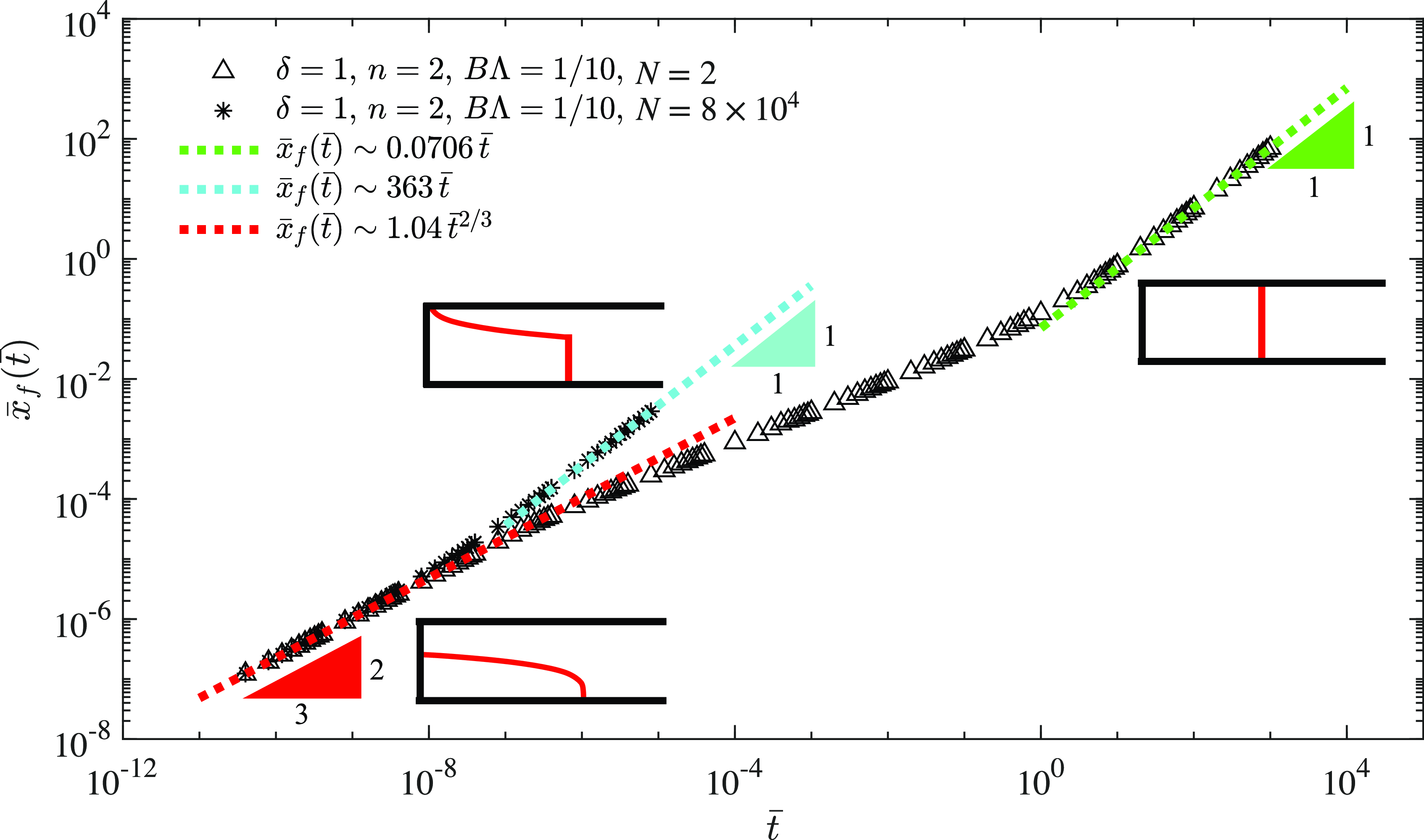
Figure 6. Time evolution of the frontal location $\bar x_f(\bar t)$
from numerically solving PDE (12) and (18), imposing
$\bar x_f(\bar t)$
from numerically solving PDE (12) and (18), imposing $\{\delta , n, B\Lambda , N\}=\{1, 2, 10^{-1}, 2\}$
and
$\{\delta , n, B\Lambda , N\}=\{1, 2, 10^{-1}, 2\}$
and $\{\delta , n, B\Lambda , N\}=\{1, 2, 10^{-1}, 8\times 10^4\}$
. The profile shape evolves from an early-time capillary film towards either a compound-wave (for
$\{\delta , n, B\Lambda , N\}=\{1, 2, 10^{-1}, 8\times 10^4\}$
. The profile shape evolves from an early-time capillary film towards either a compound-wave (for $N=8\times 10^4$
) or a shock (for
$N=8\times 10^4$
) or a shock (for $N=2$
) at late times. The asymptotic solutions for the frontal location (33) and (33) are also included as the dashed lines.
$N=2$
) at late times. The asymptotic solutions for the frontal location (33) and (33) are also included as the dashed lines.
To demonstrate the time transition from early-time to late-time self-similarities, the location of the propagating front $\bar x_f(\bar t)$
can be tracked based on the numerical solutions of PDE (12a), shown as the symbols in Figure 6. For example, for
$\bar x_f(\bar t)$
can be tracked based on the numerical solutions of PDE (12a), shown as the symbols in Figure 6. For example, for $\{\delta , n, N\, B\Lambda \}=\{1,2,8\times 10^4,10^{-1}\}$
, the time-dependent location of the propagating front
$\{\delta , n, N\, B\Lambda \}=\{1,2,8\times 10^4,10^{-1}\}$
, the time-dependent location of the propagating front $\bar x_f(\bar t)$
obeys the power-law form of
$\bar x_f(\bar t)$
obeys the power-law form of
 \begin{align} \bar x_f(\bar t) \sim 1.04\,\bar t^{2/3} \,\quad \, \mbox{for}\,\,\bar t \ll 1, \end{align}
 \begin{align} \bar x_f(\bar t) \sim 363\, \bar t \quad \mbox{for}\,\,\, \bar t \gg 1, \end{align}
and for $\{\delta , n, N, B\Lambda \}=\{1,2,2,1/10\}$
,
$\{\delta , n, N, B\Lambda \}=\{1,2,2,1/10\}$
, $\bar x_f(\bar t)$
follows
$\bar x_f(\bar t)$
follows
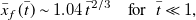 \begin{align} \bar x_f(\bar t) \sim 1.04\,\bar t^{2/3} \quad \mbox{for}\,\,\, \bar t \ll 1, \end{align}
 \begin{align} \bar x_f(\bar t) \sim 0.0706\, \bar t \quad \mbox{for}\,\,\, \bar t \gg 1. \end{align}
The PDE numerical solutions for $\bar x_f(\bar t)$
can also be compared with the early-time and late-time self-similar solutions, shown as the dashed lines in Figure 6, and good agreement appears at both the early and late times. In the SM, we also compared the appropriately rescaled profile shapes from solving the original PDE system (12a), which further verifies the existence of these early-time and late-time asymptotes. A brief description of a finite volume scheme is also included in the SM that has been used to numerically solve the nonlinear advective-diffusive system.
$\bar x_f(\bar t)$
can also be compared with the early-time and late-time self-similar solutions, shown as the dashed lines in Figure 6, and good agreement appears at both the early and late times. In the SM, we also compared the appropriately rescaled profile shapes from solving the original PDE system (12a), which further verifies the existence of these early-time and late-time asymptotes. A brief description of a finite volume scheme is also included in the SM that has been used to numerically solve the nonlinear advective-diffusive system.
2.4.2 Sharp-interface regime
When $B \gg 1$
or when
$B \gg 1$
or when $\Lambda \gg 1$
, in contrast, analytical solution (13) for saturation field reduces to
$\Lambda \gg 1$
, in contrast, analytical solution (13) for saturation field reduces to
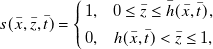 \begin{equation} s(\bar x, \bar z, \bar t) = \left \{\begin{array}{l@{\quad}l} 1, & 0 \le \bar z \le \bar h(\bar x,\bar t), \\[4pt] 0, & h(\bar x,\bar t) \lt \bar z \le 1, \end{array} \right .\quad \quad \end{equation}
for any $\alpha \ge 0$
and
$\alpha \ge 0$
and $\beta \ge 0$
, which represents an instantaneous change of fluid saturation
$\beta \ge 0$
, which represents an instantaneous change of fluid saturation $s(\bar x, \bar z, \bar t)$
across a sharp interface
$s(\bar x, \bar z, \bar t)$
across a sharp interface $\bar z=\bar h(\bar x, \bar t)$
, as shown in Figure 2. The integrals
$\bar z=\bar h(\bar x, \bar t)$
, as shown in Figure 2. The integrals $\bar I_s(\bar h)$
,
$\bar I_s(\bar h)$
, $\bar I_n(\bar h)$
and
$\bar I_n(\bar h)$
and $\bar I_w(\bar h)$
reduce to
$\bar I_w(\bar h)$
reduce to
 \begin{equation} \bar I_s(\bar h) \equiv \frac {\bar h^{2\delta /n+1}}{2\delta /n + 1}, \quad \bar I_n(\bar h) = \frac {\bar h^{2\delta +1}}{2\delta + 1}\quad \mbox{and}\quad \bar I_w(\bar h) = \frac {1-\bar h^{2\delta +1}}{2\delta + 1}. \end{equation}
We can then study the early-time and late-time asymptotic solutions for the interface shape evolution in this sharp-interface regime and the time transition. A key message is that the existence of a vertical heterogeneity ( $r_a(z) \sim r_1 z^{\delta }$
) leads to a modification of the late-time interface shape from shock or rarefaction solutions (for
$r_a(z) \sim r_1 z^{\delta }$
) leads to a modification of the late-time interface shape from shock or rarefaction solutions (for $\delta =0$
) to compound-wave solutions. The frontal location of the invading fluid
$\delta =0$
) to compound-wave solutions. The frontal location of the invading fluid $\bar x_f(\bar t)$
also adjusts accordingly. An interested reader can refer to the earlier reports of Zheng et al. (Reference Zheng, Ronge and Stone2015
b) (for
$\bar x_f(\bar t)$
also adjusts accordingly. An interested reader can refer to the earlier reports of Zheng et al. (Reference Zheng, Ronge and Stone2015
b) (for $\delta =0$
) and Hinton & Woods (Reference Hinton and Woods2018) (for
$\delta =0$
) and Hinton & Woods (Reference Hinton and Woods2018) (for $\delta =1/2$
), where two more asymptotes are identified as unconfined gravity current flows at early times and confined interfacial flows at late times. We do not repeat the detailed descriptions here.
$\delta =1/2$
), where two more asymptotes are identified as unconfined gravity current flows at early times and confined interfacial flows at late times. We do not repeat the detailed descriptions here.
3. Potential implications
It is also of interest to briefly remark on the potential implications of the model and solutions. For example, in the context of geological CO $_2$
sequestration, it is important to understand the location of the propagating front and distribution of the supercritical CO
$_2$
sequestration, it is important to understand the location of the propagating front and distribution of the supercritical CO $_2$
, when a CO
$_2$
, when a CO $_2$
plume is injected into a layer of saline aquifer. The correct result depends on the dominant physical mechanism that is related to the competition among the gravitational, pumping, and wetting and capillary forces, and the specific form of the heterogeneity of the porous layer. Quick insights can be obtained based on the value of the dimensionless parameters, and the characteristic time and length scales, imposing geophysical and operational parameters and fluids properties at reservoir conditions.
$_2$
plume is injected into a layer of saline aquifer. The correct result depends on the dominant physical mechanism that is related to the competition among the gravitational, pumping, and wetting and capillary forces, and the specific form of the heterogeneity of the porous layer. Quick insights can be obtained based on the value of the dimensionless parameters, and the characteristic time and length scales, imposing geophysical and operational parameters and fluids properties at reservoir conditions.
It has been shown in previous studies that for porous rocks with lower permeabilities, it is no longer appropriate to employ the sharp-interface flow models, as a CO $_2$
current can become significantly unsaturated due to the influence of the wetting and capillary effects (Golding et al. Reference Golding, Neufeld, Hesse and Huppert2011; Zheng & Neufeld Reference Zheng and Neufeld2019). This is also true for the spreading of CO
$_2$
current can become significantly unsaturated due to the influence of the wetting and capillary effects (Golding et al. Reference Golding, Neufeld, Hesse and Huppert2011; Zheng & Neufeld Reference Zheng and Neufeld2019). This is also true for the spreading of CO $_2$
currents in heterogeneous porous layers within regions of lower permeability, corresponding to pore sizes that are smaller than the capillary length scale. This is also demonstrated in cases (ii) and (iii) of the example calculations here with key features summarised in Table 2. It is assumed that a saline aquifer exhibits a linear variation in intrinsic permeability in the vertical direction in both cases (ii) and (iii), but the porous rock is more tight in case (iii) with much smaller pore sizes (and permeability). As a comparison, case (i) corresponds to the flow of CO
$_2$
currents in heterogeneous porous layers within regions of lower permeability, corresponding to pore sizes that are smaller than the capillary length scale. This is also demonstrated in cases (ii) and (iii) of the example calculations here with key features summarised in Table 2. It is assumed that a saline aquifer exhibits a linear variation in intrinsic permeability in the vertical direction in both cases (ii) and (iii), but the porous rock is more tight in case (iii) with much smaller pore sizes (and permeability). As a comparison, case (i) corresponds to the flow of CO $_2$
in an homogeneous layer with constant permeability, and the geophysical and operational parameters are consistent with those at the Sleipner sites. Details of the definition and physical meaning of the variables and dimensionless parameters can be found in the maintext.
$_2$
in an homogeneous layer with constant permeability, and the geophysical and operational parameters are consistent with those at the Sleipner sites. Details of the definition and physical meaning of the variables and dimensionless parameters can be found in the maintext.
Table 2. Influence of vertical heterogeneity ( $\delta$
) on the propagation of a CO
$\delta$
) on the propagation of a CO $_2$
current in a layer of saline aquifer. The geophysical and operational properties are imposed based on the CO
$_2$
current in a layer of saline aquifer. The geophysical and operational properties are imposed based on the CO $_2$
sequestration project at the Sleipner site (Golding et al. Reference Golding, Neufeld, Hesse and Huppert2011; Pegler et al. Reference Pegler, Huppert and Neufeld2014; Guo et al. Reference Guo, Zheng, Bandilla, Celia and Stone2016a; Zheng & Neufeld Reference Zheng and Neufeld2019). We have imposed
$_2$
sequestration project at the Sleipner site (Golding et al. Reference Golding, Neufeld, Hesse and Huppert2011; Pegler et al. Reference Pegler, Huppert and Neufeld2014; Guo et al. Reference Guo, Zheng, Bandilla, Celia and Stone2016a; Zheng & Neufeld Reference Zheng and Neufeld2019). We have imposed $\delta = 0$
in case (i) for an homogeneous porous layer and
$\delta = 0$
in case (i) for an homogeneous porous layer and $\delta = 1/2$
in cases (ii) and (iii) for heterogeneous porous layers with a linearly varing permeability distribution (
$\delta = 1/2$
in cases (ii) and (iii) for heterogeneous porous layers with a linearly varing permeability distribution ( $k \propto z$
), similar to previous investigations of sharp-interface flows (Huppert & Woods Reference Huppert and Woods1995; Hinton & Woods Reference Hinton and Woods2018). The geophysical parameters and fluid properties in case (i) are taken from those at the Sleipner site at reservoir conditions. By definition,
$k \propto z$
), similar to previous investigations of sharp-interface flows (Huppert & Woods Reference Huppert and Woods1995; Hinton & Woods Reference Hinton and Woods2018). The geophysical parameters and fluid properties in case (i) are taken from those at the Sleipner site at reservoir conditions. By definition, $q \equiv Q/d$
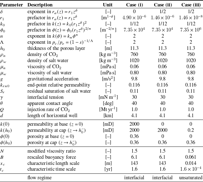
In these example calculations, it has been illustrated that the rescaled buoyancy parameter $B \equiv \Delta \rho g r_1 h_0^{\delta +1}/\gamma \, \mbox{cos}\,\theta$
can become relevant, based on the geophysical and operational parameters. Recall that
$B \equiv \Delta \rho g r_1 h_0^{\delta +1}/\gamma \, \mbox{cos}\,\theta$
can become relevant, based on the geophysical and operational parameters. Recall that $B$
measures the competition between the gravitational and capillary forces for flow in heterogeneous porous layers, and the flow of CO
$B$
measures the competition between the gravitational and capillary forces for flow in heterogeneous porous layers, and the flow of CO $_2$
becomes unsaturated for moderate and small
$_2$
becomes unsaturated for moderate and small $B$
. Since
$B$
. Since $1/B$
can also be understood as a rescaled length of the capillary fringe, physically, a small
$1/B$
can also be understood as a rescaled length of the capillary fringe, physically, a small $B$
indicates that the length of the capillary fringe now becomes comparable with the thickness of the porous layer
$B$
indicates that the length of the capillary fringe now becomes comparable with the thickness of the porous layer $h_0$
. In such a situation, the CO
$h_0$
. In such a situation, the CO $_2$
plume would distribute non-uniformly within the porous layer, and the saturation field would exhibit significant spatial variations. In this example,
$_2$
plume would distribute non-uniformly within the porous layer, and the saturation field would exhibit significant spatial variations. In this example, $B \approx 6.1$
in case (ii), while
$B \approx 6.1$
in case (ii), while $B \approx 0.061$
in case (iii), leading to completely different flow regimes with either negligible or non-negligible capillary effects. It is likely to be reasonable to employ sharp-interface flow models to make prediction on the spreading dynamics of CO
$B \approx 0.061$
in case (iii), leading to completely different flow regimes with either negligible or non-negligible capillary effects. It is likely to be reasonable to employ sharp-interface flow models to make prediction on the spreading dynamics of CO $_2$
for case (ii), while it is more appropriate to employ the unsaturated flow models for correct predictions for case (iii). We would stop the detailed discussions here by mentioning that the frontal location and saturation distribution of the CO
$_2$
for case (ii), while it is more appropriate to employ the unsaturated flow models for correct predictions for case (iii). We would stop the detailed discussions here by mentioning that the frontal location and saturation distribution of the CO $_2$
plume would adjust accordingly as injection proceeds. It is also important to remain aware that for the one-dimensional flow models to apply, the length of the current (with dimension) needs to be significantly greater than the height of the current, which must be checked eventually.
$_2$
plume would adjust accordingly as injection proceeds. It is also important to remain aware that for the one-dimensional flow models to apply, the length of the current (with dimension) needs to be significantly greater than the height of the current, which must be checked eventually.
4. Summary and final remarks
We have provided a unified theory in this work for the gravity current, interfacial and unsaturated flows in a vertically heterogeneous porous layer, a model context that could find applications in geological CO $_2$
sequestration, groundwater flow, pollutant transport, and oil and gas recovery. The theory presented in § 2 works for predominantly one-dimensional flows in porous systems with any form of vertical heterogeneity, in principle, providing that the assumption of vertical gravitational-capillary equilibrium continues to apply. We then impose power-law form of vertical heterogeneity to further demonstrate the concepts. Seven dimensionless parameters were identified, as summarised in Table 1:
$_2$
sequestration, groundwater flow, pollutant transport, and oil and gas recovery. The theory presented in § 2 works for predominantly one-dimensional flows in porous systems with any form of vertical heterogeneity, in principle, providing that the assumption of vertical gravitational-capillary equilibrium continues to apply. We then impose power-law form of vertical heterogeneity to further demonstrate the concepts. Seven dimensionless parameters were identified, as summarised in Table 1: $\delta$
and
$\delta$
and $n$
represent intrinsic features of vertical heterogeneity of the porous layer,
$n$
represent intrinsic features of vertical heterogeneity of the porous layer, $\alpha$
,
$\alpha$
, $\beta$
and
$\beta$
and $\Lambda$
characterises multi-phase Darcy flow in homogeneous porous layers,
$\Lambda$
characterises multi-phase Darcy flow in homogeneous porous layers, $N$
is the modified viscosity ratio, and
$N$
is the modified viscosity ratio, and $B$
represents the competition between the gravitational and capillary forces. The influence of these dimensionless parameters (with an emphasis on
$B$
represents the competition between the gravitational and capillary forces. The influence of these dimensionless parameters (with an emphasis on $\delta$
and
$\delta$
and $n$
) are then illustrated based on the asymptotic and numerical solutions of the saturation field, interface shape, and the frontal location.
$n$
) are then illustrated based on the asymptotic and numerical solutions of the saturation field, interface shape, and the frontal location.
In particular, when $B \ll 1$
, the model predicts a significantly unsaturated flow regime (§ 2.4.1). A capillary film solution is identified at early times by solving a nonlinear diffusive equation, which evolves towards an unsaturated current solution at late times, with the profile shape described by either a shock or a compound-wave solution. Time transition between the early-time unconfined and late-time confined self-similar solutions is then demonstrated by tracking the interface shape and frontal location. In contrast, when
$B \ll 1$
, the model predicts a significantly unsaturated flow regime (§ 2.4.1). A capillary film solution is identified at early times by solving a nonlinear diffusive equation, which evolves towards an unsaturated current solution at late times, with the profile shape described by either a shock or a compound-wave solution. Time transition between the early-time unconfined and late-time confined self-similar solutions is then demonstrated by tracking the interface shape and frontal location. In contrast, when $B \gg 1$
(or
$B \gg 1$
(or $\Lambda \gg 1$
), the model predicts a sharp-interface flow regime (§ 2.4.2), when fluid saturation changes instantaneously across a sharp fluid–fluid interface, and a gravity current solution is identified at early times, which evolves towards a shock or compound-wave solution at late times (without considering the influence of buoyancy on the frontal structure). Finally, potential implications of the model and solutions are also demonstrated, using geophysical and operational parameters in the context of geological CO
$\Lambda \gg 1$
), the model predicts a sharp-interface flow regime (§ 2.4.2), when fluid saturation changes instantaneously across a sharp fluid–fluid interface, and a gravity current solution is identified at early times, which evolves towards a shock or compound-wave solution at late times (without considering the influence of buoyancy on the frontal structure). Finally, potential implications of the model and solutions are also demonstrated, using geophysical and operational parameters in the context of geological CO $_2$
sequestration in vertically heterogeneous porous layers.
$_2$
sequestration in vertically heterogeneous porous layers.
Funding
We gratefully acknowledge funding by the Program for Professor of Special Appointment (Eastern Scholar, no. TP2020009) at Shanghai Institutions of Higher Learning.
Competing interests
The authors declare no conflict of interest.
Ethical statement
The research meets all ethical guidelines, including adherence to the legal requirements of the study country.
Data availability statement
Raw data are available from the corresponding author.
Supplementary material
The supplementary material for this article can be found at https://doi.org/10.1017/flo.2025.13.


 Open access