


1 Introduction
Let p be a prime with
 $p\geq 3$
and let
$p\geq 3$
and let
 $q=p^a$
. Let
$q=p^a$
. Let
 ${{X}}$
be a smooth proper curve of genus g defined over
${{X}}$
be a smooth proper curve of genus g defined over
 $\mathbb {F}_q$
with function field
$\mathbb {F}_q$
with function field
 $K(X)$
. We define
$K(X)$
. We define
 $G_X$
to be the absolute Galois group of
$G_X$
to be the absolute Galois group of
 $K(X)$
. Let
$K(X)$
. Let
 ${ {\rho }}:G_X \to \mathbb {C}^{\times }$
be a nontrivial continuous character. The L-function associated to
${ {\rho }}:G_X \to \mathbb {C}^{\times }$
be a nontrivial continuous character. The L-function associated to
 $\rho $
is defined by
$\rho $
is defined by
 $$ \begin{align} L(\rho,s) =\prod\frac{1}{1 - \rho(Frob_x) s^{\deg(x)}}, \\[-17pt]\nonumber\end{align} $$
with the product taken over all closed points
 $x \in X$
where
$x \in X$
where
 $\rho $
is unramified. By the Weil conjectures for curves [Reference Weil31], we know that
$\rho $
is unramified. By the Weil conjectures for curves [Reference Weil31], we know that
 $$ \begin{align*} L(\rho,s) = \prod_{i=1}^{d}(1-\alpha_i s) \in \overline{\mathbb{Z}}[s].\\[-17pt] \end{align*} $$
It is then natural to ask what we can say about the algebraic integers
 $\alpha _i$
. The Riemann hypothesis for curves tell us that
$\alpha _i$
. The Riemann hypothesis for curves tell us that
 $\lvert \alpha _i\rvert _\infty = \sqrt {q}$
for each Archimedean place. Furthermore, we know that the
$\lvert \alpha _i\rvert _\infty = \sqrt {q}$
for each Archimedean place. Furthermore, we know that the
 $\alpha _i$
are
$\alpha _i$
are
 $\ell $
-adic units for any prime
$\ell $
-adic units for any prime
 $\ell \neq p$
. This leaves us with the question: What are the p-adic valuations of the
$\ell \neq p$
. This leaves us with the question: What are the p-adic valuations of the
 $\alpha _i$
?
$\alpha _i$
?
The purpose of this article is to study the p-adic properties of
 $L(\rho ,s)$
. We prove a ‘Newton over Hodge’ result. This is in the vein of a celebrated theorem of Mazur [Reference Mazur20], which compares the Newton and Hodge polygons of an algebraic variety over
$L(\rho ,s)$
. We prove a ‘Newton over Hodge’ result. This is in the vein of a celebrated theorem of Mazur [Reference Mazur20], which compares the Newton and Hodge polygons of an algebraic variety over
 $\mathbb {F}_q$
. Our result differs from Mazur’s in that we study cohomology with coefficients in a local system. Our Hodge bound is defined using two monodromy invariants: the Swan conductor and the tame exponents. The representation
$\mathbb {F}_q$
. Our result differs from Mazur’s in that we study cohomology with coefficients in a local system. Our Hodge bound is defined using two monodromy invariants: the Swan conductor and the tame exponents. The representation
 $\rho $
is analogous to a rank
$\rho $
is analogous to a rank
 $1$
differential equation on a Riemann surface with regular singularities twisted by an exponential differential equation (i.e., a weight
$1$
differential equation on a Riemann surface with regular singularities twisted by an exponential differential equation (i.e., a weight
 $0$
twisted Hodge module in the language of Esnault, Sabbah and Yu [Reference Esnault, Sabbah and Yu9]). In this context one may define an irregular Hodge polygon [Reference Deligne, Malgrange and Ramis8, Reference Esnault, Sabbah and Yu9]. The irregular Hodge polygon agrees with the Hodge polygon we define under certain nondegeneracy hypotheses. Our result thus gives further credence to the philosophy that characteristic
$0$
twisted Hodge module in the language of Esnault, Sabbah and Yu [Reference Esnault, Sabbah and Yu9]). In this context one may define an irregular Hodge polygon [Reference Deligne, Malgrange and Ramis8, Reference Esnault, Sabbah and Yu9]. The irregular Hodge polygon agrees with the Hodge polygon we define under certain nondegeneracy hypotheses. Our result thus gives further credence to the philosophy that characteristic
 $0$
Hodge-type phenomena force p-adic bounds on lisse sheaves in characteristic p.
$0$
Hodge-type phenomena force p-adic bounds on lisse sheaves in characteristic p.
1.1 Statement of main results
To state our main result, we first introduce some monodromy invariants. The character
 $\rho $
factors uniquely as
$\rho $
factors uniquely as
 $\rho =\rho ^{wild} \otimes \chi $
, where
$\rho =\rho ^{wild} \otimes \chi $
, where
 $\left \lvert Im\left (\rho ^{wild}\right )\right \rvert =p^n$
and
$\left \lvert Im\left (\rho ^{wild}\right )\right \rvert =p^n$
and
 $\lvert Im(\chi )\rvert =N$
with
$\lvert Im(\chi )\rvert =N$
with
 $\gcd (N,p)=1$
.
$\gcd (N,p)=1$
.
-
1. (Local) Let
 $Q \in X$
be a closed point. After increasing q we may assume that Q is an
$\mathbb {F}_q$
-point. Let
$u_Q$
be a local parameter at Q. Then
$\rho $
restricts to a local representation
$\rho _Q:G_Q \to \mathbb {C}^{\times }$
, where
$G_Q$
is the absolute Galois group of
$\mathbb {F}_q((u_Q))$
. We let
$\rho ^{wild}_Q$
(resp.,
$\chi _Q$
) denote the restriction of
$\rho ^{wild}$
(resp.,
$\chi $
) to
$G_Q$
.
$Q \in X$
be a closed point. After increasing q we may assume that Q is an
$\mathbb {F}_q$
-point. Let
$u_Q$
be a local parameter at Q. Then
$\rho $
restricts to a local representation
$\rho _Q:G_Q \to \mathbb {C}^{\times }$
, where
$G_Q$
is the absolute Galois group of
$\mathbb {F}_q((u_Q))$
. We let
$\rho ^{wild}_Q$
(resp.,
$\chi _Q$
) denote the restriction of
$\rho ^{wild}$
(resp.,
$\chi $
) to
$G_Q$
.-
(a) (Swan conductors) Let
$I_Q \subset G_Q$
be the inertia subgroup at Q. There is a decreasing filtration of subgroups
$I_Q^s$
on
$I_Q$
, indexed by real numbers
$s\geq 0$
. The Swan conductor at Q is the infimum of all s such that
$I_Q^s \subset \ker (\rho _Q)$
[Reference Katz13, Chapter 1]. We denote the Swan conductor by
${ {s_Q}}$
. Note that
$s_Q=0$
if and only if
$\rho _Q^{wild}$
is unramified. -
(b) (Tame exponents) After increasing q we may assume that
$\chi _Q$
is totally ramified at Q. There exists
$e_Q \in \frac {1}{q-1}\mathbb {Z}$
such that
$G_Q$
acts on
$t_Q^{e_Q}$
by
$\chi _Q$
. Note that
$e_Q$
is unique up to addition by an integer.-
○ The exponent of
$\chi $
at Q is the equivalence class
${ {\mathbf {e}_Q}}$
of
$e_Q$
in
$ \frac {1}{q-1}\mathbb {Z}/ \mathbb {Z}$
. -
○ We define
${ {\epsilon _Q}}$
to be the unique integer between
$0$
and
$q-2$
such that
$\frac {\epsilon _Q}{q-1} \in \mathbf {e}_Q$
. -
○ Write
$\epsilon _Q=e_{Q,0} + e_{Q,1}p + \dotsb +e_{Q,a-1} p^{a-1}$
, where
$0 \leq e_{Q,i}\leq p-1$
. We define
${ {\omega _Q}}=\sum e_{Q,i}$
, the sum of the p-adic digits of
$\epsilon _Q$
. Note that
$\omega _Q=0$
if and only if
$\chi _Q$
is unramified.
-
We refer to the tuple
$R_Q=\left (s_Q, \mathbf {e}_Q, \epsilon _Q, \omega _Q\right )$
as a ramification datum and
$T_Q=\left (\mathbf {e}_Q,\epsilon _Q,\omega _Q\right )$
as a tame ramification datum. We define the sets
$$ \begin{align*} S_{Q} &= \begin{cases} \emptyset & s_Q=0, \\ \left\{ \frac{1}{s_{Q}}, \dotsc, \frac{s_{Q}-1}{s_{Q}}\right\}, & s_Q \neq 0 \text{ and } \omega_Q =0, \\ \left\{ \frac{1}{s_{Q}}- \frac{\omega_{Q}}{as_{Q}\left(p-1\right)}, \dotsc, \frac{s_{Q}}{s_{Q}}- \frac{\omega_{Q}}{as_{Q}\left(p-1\right)}\right\}, & s_Q \neq 0 \text{ and } \omega_Q \neq 0. \end{cases} \\[-17pt]\end{align*} $$
-
-
2. (Global) Let
${ {\tau _1,\dotsc ,\tau _{\mathbf {m}}}}$
be the points at which
$\rho $
ramifies and let
$\mathbf {n}\leq { {\mathbf {m}}}$
be such that
$\tau _1, \dotsc , \tau _{\mathbf {n}}$
are the points at which
$\chi $
ramifies. We define This is a global invariant built up from the p-adic properties of the local exponents. One can show that
$$ \begin{align*} {{\Omega_\rho}} &= \frac{1}{a(p-1)} \sum_{i=1}^{\mathbf{n}} \omega_{\tau_i}.\\[-17pt] \end{align*} $$
$\Omega _\rho \in \mathbb {Z}_{\geq 0}$
(see Section 5.3.2).


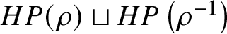
Using these invariants, we define the Hodge polygon
 ${ {HP(\rho )}}$
to be the polygon whose slopes are
${ {HP(\rho )}}$
to be the polygon whose slopes are
 $$ \begin{align*} \{\underbrace{0,\dotsc,0}_{g-1+\mathbf{m}-\Omega_\rho} \}\sqcup \{\underbrace{1,\dotsc,1}_{g-1+\mathbf{m}-\mathbf{n} + \Omega_\rho} \} \sqcup \left ( \bigsqcup_{i=1}^{\mathbf{m}} S_{\tau_i} \right ), \end{align*} $$
where
 $\sqcup $
denotes a disjoint union. We can now state our main result:
$\sqcup $
denotes a disjoint union. We can now state our main result:
Theorem 1.1. The q-adic Newton polygon
 $NP_q(L(\rho ,s))$
lies above the Hodge polygon
$NP_q(L(\rho ,s))$
lies above the Hodge polygon
 $HP(\rho )$
.
$HP(\rho )$
.
Remark 1.2. It is worth mentioning that
 $HP(\rho )$
and
$HP(\rho )$
and
 $NP_q(L(\rho ,s))$
have the same endpoints. To see this, first note that the x-coordinates of the endpoints of both polygons are
$NP_q(L(\rho ,s))$
have the same endpoints. To see this, first note that the x-coordinates of the endpoints of both polygons are
 $g-1+\mathbf {m} + \sum s_Q$
. For
$g-1+\mathbf {m} + \sum s_Q$
. For
 $NP_q(L(\rho ,s))$
this follows from the Euler–Poincaré formula [Reference Katz13, Section 2.3.1], and for
$NP_q(L(\rho ,s))$
this follows from the Euler–Poincaré formula [Reference Katz13, Section 2.3.1], and for
 $HP(\rho )$
it is clear from the definition. Next let
$HP(\rho )$
it is clear from the definition. Next let
 $\left (s_{\tau _i}', \mathbf {e}_{\tau _i}', \epsilon _{\tau _i}', \omega _{\tau _i}'\right )$
be the ramification datum associated to
$\left (s_{\tau _i}', \mathbf {e}_{\tau _i}', \epsilon _{\tau _i}', \omega _{\tau _i}'\right )$
be the ramification datum associated to
 $\rho ^{-1}$
at
$\rho ^{-1}$
at
 ${\tau _i}$
. Then we have
${\tau _i}$
. Then we have
 $s_{\tau _i}'=s_{\tau _i}$
and
$s_{\tau _i}'=s_{\tau _i}$
and
 $\mathbf {e}_{\tau _i}'=-\mathbf {e}_{\tau _i}$
. From this we see that
$\mathbf {e}_{\tau _i}'=-\mathbf {e}_{\tau _i}$
. From this we see that
 $\omega _{\tau _{i}}'=a(p-1)-\omega _{\tau _{i}}$
for
$\omega _{\tau _{i}}'=a(p-1)-\omega _{\tau _{i}}$
for
 $1\leq i \leq \mathbf {n}$
and
$1\leq i \leq \mathbf {n}$
and
 $\omega _{\tau _i}'=0$
for
$\omega _{\tau _i}'=0$
for
 $i>\mathbf {n}$
, which implies
$i>\mathbf {n}$
, which implies
 $\Omega _{\rho ^{-1}}=\mathbf {n}-\Omega _{\rho }$
. Thus, for every slope
$\Omega _{\rho ^{-1}}=\mathbf {n}-\Omega _{\rho }$
. Thus, for every slope
 $\alpha $
of
$\alpha $
of
 $HP(\rho )$
, there is a corresponding slope
$HP(\rho )$
, there is a corresponding slope
 $1-\alpha $
of
$1-\alpha $
of
 $HP\left (\rho ^{-1}\right )$
. Similarly, by Poincaré duality we know that for every slope
$HP\left (\rho ^{-1}\right )$
. Similarly, by Poincaré duality we know that for every slope
 $\alpha $
of
$\alpha $
of
 $NP_q(L(\rho ,s))$
, there is a corresponding slope
$NP_q(L(\rho ,s))$
, there is a corresponding slope
 $1-\alpha $
of
$1-\alpha $
of
 $NP_q\left (L\left (\rho ^{-1},s\right )\right )$
. It follows that the y-coordinates of the endpoints of
$NP_q\left (L\left (\rho ^{-1},s\right )\right )$
. It follows that the y-coordinates of the endpoints of
 $HP(\rho )\sqcup HP\left (\rho ^{-1}\right )$
and
$HP(\rho )\sqcup HP\left (\rho ^{-1}\right )$
and
 $NP_q(L(\rho ,s))\sqcup NP_q\left (L\left (\rho ^{-1},s\right )\right )$
agree. By applying Theorem 1.1 to
$NP_q(L(\rho ,s))\sqcup NP_q\left (L\left (\rho ^{-1},s\right )\right )$
agree. By applying Theorem 1.1 to
 $\rho $
and
$\rho $
and
 $\rho ^{-1}$
, we see that the endpoints of
$\rho ^{-1}$
, we see that the endpoints of
 $HP(\rho )$
and
$HP(\rho )$
and
 $NP_q(L(\rho ,s))$
are the same.
$NP_q(L(\rho ,s))$
are the same.
Remark 1.3. When
 $\rho $
factors through an Artin–Schreier cover, Theorem 1.1 is due to previous work of the author [Reference Kramer-Miller15].
$\rho $
factors through an Artin–Schreier cover, Theorem 1.1 is due to previous work of the author [Reference Kramer-Miller15].
Remark 1.4. The only other case where parts of Theorem 1.1 were previously known is when
 $X=\mathbb {P}^1$
and
$X=\mathbb {P}^1$
and
 $\rho $
is unramified outside of
$\rho $
is unramified outside of
 $\mathbb {G}_m$
. Work of Adolphson and Sperber [Reference Adolphson and Sperber2, Reference Adolphson and Sperber3] studies the case when
$\mathbb {G}_m$
. Work of Adolphson and Sperber [Reference Adolphson and Sperber2, Reference Adolphson and Sperber3] studies the case when
 $\lvert Im(\rho )\rvert =pN$
and
$\lvert Im(\rho )\rvert =pN$
and
 $\gcd (p,N)=1$
. We note that the work of Adolphson and Sperber treats the case of higher-dimensional tori as well. These groundbreaking methods were applied to the case when
$\gcd (p,N)=1$
. We note that the work of Adolphson and Sperber treats the case of higher-dimensional tori as well. These groundbreaking methods were applied to the case when
 $\rho $
is totally wild by Liu and Wei in [Reference Liu and Wei18], introducing ideas from Artin–Schreier–Witt theory. For
$\rho $
is totally wild by Liu and Wei in [Reference Liu and Wei18], introducing ideas from Artin–Schreier–Witt theory. For
 $\rho $
with arbitrary image there are some results by Liu [Reference Liu17], under strict conditions on the wild part of
$\rho $
with arbitrary image there are some results by Liu [Reference Liu17], under strict conditions on the wild part of
 $\rho $
(this case corresponds to Heilbronn sums).
$\rho $
(this case corresponds to Heilbronn sums).
To the best of our knowledge, Theorem 1.1 was completely unknown outside of the situations described in Remarks 1.3 and 1.4.
Example 1.5. Let
 $X=\mathbb {P}^1_{\mathbb {F}_q}$
and let
$X=\mathbb {P}^1_{\mathbb {F}_q}$
and let
 $\tau _1,\dotsc ,\tau _{4}$
be the points where
$\tau _1,\dotsc ,\tau _{4}$
be the points where
 $\rho $
ramifies. Assume
$\rho $
ramifies. Assume
 $\lvert Im(\rho )\rvert =2p^n$
and that
$\lvert Im(\rho )\rvert =2p^n$
and that
 $\rho $
is totally ramified at each
$\rho $
is totally ramified at each
 $\tau _i$
(i.e., the inertia group at
$\tau _i$
(i.e., the inertia group at
 $\tau _i$
is equal to
$\tau _i$
is equal to
 $Im(\rho )$
). Let
$Im(\rho )$
). Let
 $f:E \to X$
be the genus
$f:E \to X$
be the genus
 $1$
curve over which
$1$
curve over which
 $\chi $
trivialises and let
$\chi $
trivialises and let
 $\upsilon _i=f^{-1}(\tau _i)$
. Consider the restriction
$\upsilon _i=f^{-1}(\tau _i)$
. Consider the restriction
 $\rho _E=\rho \rvert _{G_E}$
. Let
$\rho _E=\rho \rvert _{G_E}$
. Let
 $(s_i, \mathbf {e}_i, \epsilon _i, \omega _i)$
be the ramification datum of
$(s_i, \mathbf {e}_i, \epsilon _i, \omega _i)$
be the ramification datum of
 $\rho $
at
$\rho $
at
 $\tau _i$
and let
$\tau _i$
and let
 $\left (s_i', \mathbf {e}_i', \epsilon _i', \omega _i'\right )$
be the ramification datum of
$\left (s_i', \mathbf {e}_i', \epsilon _i', \omega _i'\right )$
be the ramification datum of
 $\rho _E$
at
$\rho _E$
at
 $\upsilon _i$
. By Theorem 1.1 we know that
$\upsilon _i$
. By Theorem 1.1 we know that
 $NP_q(L(\rho _E,s))$
lies above
$NP_q(L(\rho _E,s))$
lies above
 $$ \begin{align*} HP(\rho_E)&= \{0,0,0,0 \}\sqcup \{1,1,1,1 \} \sqcup \left ( \bigsqcup_{i=1}^4 \left\{\frac{1}{2s_i}, \dotsc, \frac{2s_i-1}{2s_i}\right\} \right ). \end{align*} $$
This follows by recognising that
 $s_i'=2s_i$
and
$s_i'=2s_i$
and
 $\omega _i'=0$
. The factorisation
$\omega _i'=0$
. The factorisation
 $L(\rho _E,s)=L(\rho ,s)L\left (\rho ^{wild},s\right )$
corresponds to a ‘decomposition’ of
$L(\rho _E,s)=L(\rho ,s)L\left (\rho ^{wild},s\right )$
corresponds to a ‘decomposition’ of
 $HP(\rho _E)$
into two Hodge polygons, one giving a lower bound for
$HP(\rho _E)$
into two Hodge polygons, one giving a lower bound for
 $NP_q(L(\rho ,s))$
and the other for
$NP_q(L(\rho ,s))$
and the other for
 $NP_q\left (L\left (\rho ^{wild},s\right )\right )$
. We have
$NP_q\left (L\left (\rho ^{wild},s\right )\right )$
. We have
 $\omega _i=\frac {a\left (p-1\right )}{2}$
for each i and
$\omega _i=\frac {a\left (p-1\right )}{2}$
for each i and
 $\Omega _\rho =2$
. This allows us to compute the Hodge polygons as
$\Omega _\rho =2$
. This allows us to compute the Hodge polygons as
 $$ \begin{align*} HP(\rho)&= \{0,1\} \sqcup \left ( \bigsqcup_{i=1}^4\left \{\frac{1}{2s_i}, \frac{3}{2s_i}, \dotsc, \frac{2s_i-1}{2s_i}\right\} \right ),\\ HP\left(\rho^{wild}\right) &= \{0,0,0 \}\sqcup \{1,1,1 \} \sqcup \left ( \bigsqcup_{i=1}^4 \left\{\frac{1}{s_i}, \dotsc, \frac{s_i-1}{s_i}\right\} \right ), \end{align*} $$
so that
 $HP(\rho _E)=HP(\rho )\sqcup HP\left (\rho ^{wild}\right )$
. More generally, we will obtain similar decompositions of the Hodge bounds as long as
$HP(\rho _E)=HP(\rho )\sqcup HP\left (\rho ^{wild}\right )$
. More generally, we will obtain similar decompositions of the Hodge bounds as long as
 $Im(\chi )\mid p-1$
.
$Im(\chi )\mid p-1$
.
1.1.1 Newton polygons of abelian covers of curves
Theorem 1.1 also has interesting consequences for Newton polygons of cyclic covers of curves. Let
 $G=\mathbb {Z}/Np^n\mathbb {Z}$
, where N is coprime to p. Let
$G=\mathbb {Z}/Np^n\mathbb {Z}$
, where N is coprime to p. Let
 $f: C \to X$
be a G-cover ramified over
$f: C \to X$
be a G-cover ramified over
 $\tau _1,\dotsc ,\tau _{\mathbf {m}}$
. We let
$\tau _1,\dotsc ,\tau _{\mathbf {m}}$
. We let
 $H^1_{cris}(X) \ \left (\text {resp., } H^1_{cris}(C)\right )$
be the crystalline cohomology of X (resp., C). For a character
$H^1_{cris}(X) \ \left (\text {resp., } H^1_{cris}(C)\right )$
be the crystalline cohomology of X (resp., C). For a character
 $\rho $
of G, we let
$\rho $
of G, we let
 $H^1_{cris}(C)^{\rho }$
be the
$H^1_{cris}(C)^{\rho }$
be the
 $\rho $
-isotypical subspace for the action of G on
$\rho $
-isotypical subspace for the action of G on
 $H^1_{cris}(C)$
. Let
$H^1_{cris}(C)$
. Let
 $NP_C \ \left (\text {resp. } NP_X \text { and } NP_C^{\rho }\right )$
denote the q-adic Newton polygon of
$NP_C \ \left (\text {resp. } NP_X \text { and } NP_C^{\rho }\right )$
denote the q-adic Newton polygon of
 $\det \left (1-s\text {F}\mid H^1_{cris}(C)\right ) \ \left (\text {resp., } \det \left (1-s\text {F}\mid H^1_{cris}(X)\right ) \text { and } \det \left (1-s\text {F}\mid H^1_{cris}(C)^{\rho }\right )\right )$
. We are interested in the following question: To what extent can we determine
$\det \left (1-s\text {F}\mid H^1_{cris}(C)\right ) \ \left (\text {resp., } \det \left (1-s\text {F}\mid H^1_{cris}(X)\right ) \text { and } \det \left (1-s\text {F}\mid H^1_{cris}(C)^{\rho }\right )\right )$
. We are interested in the following question: To what extent can we determine
 $NP_C$
from
$NP_C$
from
 $NP_X$
and the ramification invariants of f? The most basic result is the Riemann–Hurwitz formula, which determines the dimension of
$NP_X$
and the ramification invariants of f? The most basic result is the Riemann–Hurwitz formula, which determines the dimension of
 $H^1_{cris}(C)$
from
$H^1_{cris}(C)$
from
 $H^1_{cris}(X)$
and the ramification invariants. When
$H^1_{cris}(X)$
and the ramification invariants. When
 $N=1$
, there is also the Deuring–Shafarevich formula [Reference Crew7], which determines the number of slope
$N=1$
, there is also the Deuring–Shafarevich formula [Reference Crew7], which determines the number of slope
 $0$
segments in
$0$
segments in
 $NP_C$
. In general, however, a precise formula for the slopes of
$NP_C$
. In general, however, a precise formula for the slopes of
 $NP_C$
seems impossible. Instead, the best we may hope for are estimates. To connect this problem to Theorem 1.1, recall the decomposition
$NP_C$
seems impossible. Instead, the best we may hope for are estimates. To connect this problem to Theorem 1.1, recall the decomposition
 $$ \begin{align} \det\left(1-s\text{F}\mid H^1_{cris}(C)\right)&= \det\left(1-s\text{F}\mid H^1_{cris}(X)\right) \prod_{\rho} \det\left(1-s\text{F}\mid H^1_{cris}(C)^{\rho}\right), \end{align} $$
where
 $\rho $
varies over the nontrivial characters
$\rho $
varies over the nontrivial characters
 $\mathbb {Z}/Np^n\mathbb {Z} \to \mathbb {C}^{\times }$
. By the Lefschetz trace formula we know
$\mathbb {Z}/Np^n\mathbb {Z} \to \mathbb {C}^{\times }$
. By the Lefschetz trace formula we know
 $L(\rho ,s)=\det \left (1-s\text {F}\mid H^1_{cris}(C)^{\rho }\right )$
. Thus, Theorem 1.1 gives lower bounds for
$L(\rho ,s)=\det \left (1-s\text {F}\mid H^1_{cris}(C)^{\rho }\right )$
. Thus, Theorem 1.1 gives lower bounds for
 $NP_C$
using equation (2).
$NP_C$
using equation (2).
Consider the case when
 $N=1$
, so that
$N=1$
, so that
 $G=\mathbb {Z}/p^n\mathbb {Z}$
. Let
$G=\mathbb {Z}/p^n\mathbb {Z}$
. Let
 $r_i$
be the ramification index of a point of C above
$r_i$
be the ramification index of a point of C above
 $\tau _i$
and define
$\tau _i$
and define
 $$ \begin{align*} \Omega = \sum_{i=1}^{\mathbf{m}} p^{n-r_i}\left(p^{r_i}-1\right). \end{align*} $$
For
 $j=1,\dotsc ,n$
, let
$j=1,\dotsc ,n$
, let
 $C_j$
be the cover of X corresponding to the subgroup
$C_j$
be the cover of X corresponding to the subgroup
 $p^{n-j}\mathbb {Z} \big / p^n\mathbb {Z} \subset G$
. Fix a point
$p^{n-j}\mathbb {Z} \big / p^n\mathbb {Z} \subset G$
. Fix a point
 $x_i(j)\in C_j$
above
$x_i(j)\in C_j$
above
 $\tau _i$
; this gives a local field extension of
$\tau _i$
; this gives a local field extension of
 $\mathbb {F}_q\left (\left (t_{\tau _i}\right )\right )$
. We let
$\mathbb {F}_q\left (\left (t_{\tau _i}\right )\right )$
. We let
 $s_{\tau _i}(j)$
denote the largest upper numbering ramification break of this extension.
$s_{\tau _i}(j)$
denote the largest upper numbering ramification break of this extension.
Corollary 1.6. The Newton polygon
 $NP_C$
lies above the polygon whose slopes are the multiset
$NP_C$
lies above the polygon whose slopes are the multiset
 $$ \begin{align*} NP_X \sqcup \{\underbrace{0,\dotsc,0}_{(p^n-1)(g-1)+\Omega}, \underbrace{1,\dotsc,1}_{(p^n-1)(g-1)+\Omega}\} \sqcup \left(\bigsqcup_{i=1}^{\mathbf{m}} \bigsqcup_{j=1}^n p^{j-1}(p-1)\times \left\{\frac{1}{s_{\tau_i}(j)}, \dotsc, \frac{s_{\tau_i}(j)-1}{s_{\tau_i}(j)} \right\}\right), \end{align*} $$
where we take
 $\left \{\frac {1}{s_{\tau _i}\left (j\right )}, \dotsc , \frac {s_{\tau _i}\left (j\right )-1}{s_{\tau _i}\left (j\right )} \right \}$
to be the empty set when
$\left \{\frac {1}{s_{\tau _i}\left (j\right )}, \dotsc , \frac {s_{\tau _i}\left (j\right )-1}{s_{\tau _i}\left (j\right )} \right \}$
to be the empty set when
 $s_{\tau _i}(j)=0$
.
$s_{\tau _i}(j)=0$
.
Remark 1.7. When
 $N>1$
, we can obtain a complicated bound for
$N>1$
, we can obtain a complicated bound for
 $NP_C$
from Theorem 1.1 and equation (2). Alternatively, we can replace X with the intermediate curve
$NP_C$
from Theorem 1.1 and equation (2). Alternatively, we can replace X with the intermediate curve
 $X^{tame}$
satisfying
$X^{tame}$
satisfying
 $Gal\left (C/X^{tame}\right )=\mathbb {Z}/p^n\mathbb {Z}$
and then apply Corollary 1.6 to the cover
$Gal\left (C/X^{tame}\right )=\mathbb {Z}/p^n\mathbb {Z}$
and then apply Corollary 1.6 to the cover
 $C \to X^{tame}$
to obtain a bound. Both bounds are the same.
$C \to X^{tame}$
to obtain a bound. Both bounds are the same.
1.2 Outline of proof
The classical approaches to studying p-adic properties of exponential sums on tori no longer work when one considers more general curves. Instead, we have to expand on the methods developed in earlier work of the author on exponential sums on curves [Reference Kramer-Miller15]. We use the Monsky trace formula (see Section 7.1). This trace formula allows us to compute
 $L(\rho ,s)$
by studying Fredholm determinants of certain operators. More precisely, let
$L(\rho ,s)$
by studying Fredholm determinants of certain operators. More precisely, let
 $V=X-\{\tau _1,\dotsc ,\tau _{\mathbf {m}} \}$
and let
$V=X-\{\tau _1,\dotsc ,\tau _{\mathbf {m}} \}$
and let
 $\overline {B}$
be the coordinate ring of V. Let L be a finite extension of
$\overline {B}$
be the coordinate ring of V. Let L be a finite extension of
 $\mathbb {Q}_p$
whose residue field is
$\mathbb {Q}_p$
whose residue field is
 $\mathbb {F}_q$
such that the image of
$\mathbb {F}_q$
such that the image of
 $\rho $
is contained in
$\rho $
is contained in
 $L^{\times }$
. Let
$L^{\times }$
. Let
 $B^{\dagger }$
be the ring of integral overconvergent functions on a formal lifting of
$B^{\dagger }$
be the ring of integral overconvergent functions on a formal lifting of
 $\overline {B}$
over
$\overline {B}$
over
 $\mathcal {O}_L$
(see Section 3). For example, if
$\mathcal {O}_L$
(see Section 3). For example, if
 $V=\mathbb {A}^1$
, then
$V=\mathbb {A}^1$
, then
 $B^{\dagger }=\mathcal {O}_L\left \langle t \right \rangle ^{\dagger }$
(i.e.,
$B^{\dagger }=\mathcal {O}_L\left \langle t \right \rangle ^{\dagger }$
(i.e.,
 $B^{\dagger }$
is the ring of power series with integral coefficients that converge beyond the closed unit disc). Choose an endomorphism
$B^{\dagger }$
is the ring of power series with integral coefficients that converge beyond the closed unit disc). Choose an endomorphism
 $\sigma : B^{\dagger } \to B^{\dagger }$
that lifts the q-power Frobenius of
$\sigma : B^{\dagger } \to B^{\dagger }$
that lifts the q-power Frobenius of
 $\overline {B}$
. Using
$\overline {B}$
. Using
 $\sigma $
, we define an operator
$\sigma $
, we define an operator
 $U_q: B^{\dagger }\to B^{\dagger }$
, which is the composition of a trace map
$U_q: B^{\dagger }\to B^{\dagger }$
, which is the composition of a trace map
 $Tr:B^{\dagger }\to \sigma \left (B^{\dagger }\right )$
with
$Tr:B^{\dagger }\to \sigma \left (B^{\dagger }\right )$
with
 $\frac {1}{q}\sigma ^{-1}$
.
$\frac {1}{q}\sigma ^{-1}$
.
The Galois representation
 $\rho $
corresponds to a unit-root overconvergent F-crystal of rank
$\rho $
corresponds to a unit-root overconvergent F-crystal of rank
 $1$
. This is a
$1$
. This is a
 $B^{\dagger }$
-module
$B^{\dagger }$
-module
 $M=B^{\dagger } e_0$
and a
$M=B^{\dagger } e_0$
and a
 $B^{\dagger }$
-linear isomorphism
$B^{\dagger }$
-linear isomorphism
 $\varphi : M \otimes _{\sigma } B^{\dagger } \to M$
. Note that this F-crystal is determined entirely by
$\varphi : M \otimes _{\sigma } B^{\dagger } \to M$
. Note that this F-crystal is determined entirely by
 $\alpha \in B^{\dagger }$
satisfying
$\alpha \in B^{\dagger }$
satisfying
 $\varphi (e_0 \otimes 1) = \alpha e_0$
. We refer to
$\varphi (e_0 \otimes 1) = \alpha e_0$
. We refer to
 $\alpha $
as the Frobenius structure of M. In our specific setup (see Section 3), the Monsky trace formula can be written as
$\alpha $
as the Frobenius structure of M. In our specific setup (see Section 3), the Monsky trace formula can be written as
 $$ \begin{align*} L(\rho,s) &= \frac{\det\left(1-sU_q \circ \alpha \mid B^{\dagger}\right)} {\det\left(1-sqU_q \circ \alpha \mid B^{\dagger}\right)}, \end{align*} $$
where we regard
 $\alpha $
as the ‘multiplication by
$\alpha $
as the ‘multiplication by
 $\alpha $
’ map on
$\alpha $
’ map on
 $B^{\dagger }$
. Thus, we need to understand the operator
$B^{\dagger }$
. Thus, we need to understand the operator
 $U_q \circ \alpha $
. Let us outline how we study this operator.
$U_q \circ \alpha $
. Let us outline how we study this operator.
1.2.1 Lifting the Frobenius endomorphism
Both
 $U_q$
and
$U_q$
and
 $\alpha $
depend on the choice of Frobenius endomorphism
$\alpha $
depend on the choice of Frobenius endomorphism
 $\sigma $
. When
$\sigma $
. When
 $V=\mathbb {G}_m$
, the ring
$V=\mathbb {G}_m$
, the ring
 $B^{\dagger }$
is
$B^{\dagger }$
is
 $\mathcal {O}_L\langle t \rangle ^{\dagger }$
, and the natural choice for
$\mathcal {O}_L\langle t \rangle ^{\dagger }$
, and the natural choice for
 $\sigma $
sends t to
$\sigma $
sends t to
 $t^q$
. However, no such natural choice exists for higher-genus curves. Our approach is to pick a convenient mapping
$t^q$
. However, no such natural choice exists for higher-genus curves. Our approach is to pick a convenient mapping
 $\eta :X \to \mathbb {P}^1$
and then pull back the Frobenius
$\eta :X \to \mathbb {P}^1$
and then pull back the Frobenius
 $t \mapsto t^q$
along
$t \mapsto t^q$
along
 $\eta $
. We take
$\eta $
. We take
 $\eta $
to be a tamely ramified map that is étale outside of
$\eta $
to be a tamely ramified map that is étale outside of
 $\{0,1,\infty \}$
. We may further assume that
$\{0,1,\infty \}$
. We may further assume that
 $\eta (\tau _i) \in \{0,\infty \}$
and the ramification index of every point in
$\eta (\tau _i) \in \{0,\infty \}$
and the ramification index of every point in
 $\eta ^{-1}(1)$
is
$\eta ^{-1}(1)$
is
 $p-1$
(see Lemma 3.1). This leaves us with two types of local Frobenius endomorphisms. For
$p-1$
(see Lemma 3.1). This leaves us with two types of local Frobenius endomorphisms. For
 $Q \in X$
with
$Q \in X$
with
 $\eta (Q)\in \{0,\infty \}$
, we may take the local parameter at Q to look like
$\eta (Q)\in \{0,\infty \}$
, we may take the local parameter at Q to look like
 $u_Q=t^{\pm \frac {1}{e_Q}}$
, where
$u_Q=t^{\pm \frac {1}{e_Q}}$
, where
 $e_Q$
is the ramification index at Q. In particular, the Frobenius endomorphism sends
$e_Q$
is the ramification index at Q. In particular, the Frobenius endomorphism sends
 $u_Q \mapsto u_Q^q$
. If
$u_Q \mapsto u_Q^q$
. If
 $\eta (Q)=1$
, we take the local parameter to look like
$\eta (Q)=1$
, we take the local parameter to look like
 $u_Q=\sqrt [p-1]{t-1}$
. Thus, the Frobenius endomorphism sends
$u_Q=\sqrt [p-1]{t-1}$
. Thus, the Frobenius endomorphism sends
 $u_Q \mapsto \sqrt [p-1]{\left (u_Q^{p-1}+1\right )^{p}-1}$
. In Section 4 we study
$u_Q \mapsto \sqrt [p-1]{\left (u_Q^{p-1}+1\right )^{p}-1}$
. In Section 4 we study
 $U_q$
for both types of local Frobenius endomorphisms, and in Section 5.2 we study the local versions of the Frobenius structure
$U_q$
for both types of local Frobenius endomorphisms, and in Section 5.2 we study the local versions of the Frobenius structure
 $\alpha $
.
$\alpha $
.
1.2.2 The problem of ath roots of
$U_q\circ \alpha $

To obtain the correct estimates of
 $\det \left (1-sU_q \circ \alpha \mid B^{\dagger }\right )$
, it is necessary to work with an ath root of
$\det \left (1-sU_q \circ \alpha \mid B^{\dagger }\right )$
, it is necessary to work with an ath root of
 $U_q\circ \alpha $
. That is, we need an element
$U_q\circ \alpha $
. That is, we need an element
 $\alpha _0 \in B^{\dagger }$
and a
$\alpha _0 \in B^{\dagger }$
and a
 $U_p$
operator (this is analogous to the
$U_p$
operator (this is analogous to the
 $U_q$
operator, but for liftings of the p-power endomorphism) such that
$U_q$
operator, but for liftings of the p-power endomorphism) such that
 $\left (U_p\circ \alpha _0\right )^a=U_q\circ \alpha $
. However, this ath root is only guaranteed to exist if the order of
$\left (U_p\circ \alpha _0\right )^a=U_q\circ \alpha $
. However, this ath root is only guaranteed to exist if the order of
 $Im(\chi )$
divides
$Im(\chi )$
divides
 $p-1$
(see Section 5.1). This presents a major technical obstacle. The solution is to consider
$p-1$
(see Section 5.1). This presents a major technical obstacle. The solution is to consider
 $ \rho ^{wild}\otimes \bigoplus \limits _{j=0}^{a-1}\chi ^{\otimes p^j}$
, which is a restriction of scalars of
$ \rho ^{wild}\otimes \bigoplus \limits _{j=0}^{a-1}\chi ^{\otimes p^j}$
, which is a restriction of scalars of
 $\rho $
. The L-functions of each summand are Galois conjugate, and thus have the same Newton polygon. We can then study an operator
$\rho $
. The L-functions of each summand are Galois conjugate, and thus have the same Newton polygon. We can then study an operator
 $U_p \circ N$
, where N is the Frobenius structure of the F-crystal associated to
$U_p \circ N$
, where N is the Frobenius structure of the F-crystal associated to
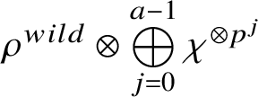 $ \rho ^{wild}\otimes \bigoplus \limits _{j=0}^{a-1}\chi ^{\otimes p^j}$
. This is similar to the idea used in Adolphson and Sperber’s study of twisted exponential sums on tori [Reference Adolphson and Sperber2]. They present it in an ad hoc manner, but the underlying idea is to study
$ \rho ^{wild}\otimes \bigoplus \limits _{j=0}^{a-1}\chi ^{\otimes p^j}$
. This is similar to the idea used in Adolphson and Sperber’s study of twisted exponential sums on tori [Reference Adolphson and Sperber2]. They present it in an ad hoc manner, but the underlying idea is to study
 $ \rho ^{wild}\otimes \bigoplus \limits _{j=0}^{a-1}\chi ^{\otimes p^j}$
in lieu of
$ \rho ^{wild}\otimes \bigoplus \limits _{j=0}^{a-1}\chi ^{\otimes p^j}$
in lieu of
 $\rho $
.
$\rho $
.
1.2.3 Global to local computations
When V is
 $\mathbb {G}_m$
or
$\mathbb {G}_m$
or
 $\mathbb {A}^1$
, the ring
$\mathbb {A}^1$
, the ring
 $B^{\dagger }$
is just
$B^{\dagger }$
is just
 $\mathcal {O}_L\left \langle t \right \rangle ^{\dagger }$
or
$\mathcal {O}_L\left \langle t \right \rangle ^{\dagger }$
or
 $\mathcal {O}_L\left \langle t,t^{-1} \right \rangle ^{\dagger }$
. In both cases, it is relatively easy to study operators on
$\mathcal {O}_L\left \langle t,t^{-1} \right \rangle ^{\dagger }$
. In both cases, it is relatively easy to study operators on
 $B^{\dagger }$
. The situation is more complex for higher-genus curves. Our approach to make sense of
$B^{\dagger }$
. The situation is more complex for higher-genus curves. Our approach to make sense of
 $B^{\dagger }$
is to ‘expand’ each function around the
$B^{\dagger }$
is to ‘expand’ each function around the
 $\tau _i$
(and some other auxiliary points). Namely, let
$\tau _i$
(and some other auxiliary points). Namely, let
 $t_i\in B^{\dagger }$
be a function whose reduction in
$t_i\in B^{\dagger }$
be a function whose reduction in
 $\overline {B}$
has a simple zero at
$\overline {B}$
has a simple zero at
 $\tau _i$
. We let
$\tau _i$
. We let
 $\mathcal {O}_{\mathcal {E}_i^{\dagger }}$
be the ring of formal Laurent series in
$\mathcal {O}_{\mathcal {E}_i^{\dagger }}$
be the ring of formal Laurent series in
 $t_i$
that converge on an annulus
$t_i$
that converge on an annulus
 $r<\lvert t_i\rvert _p<1$
(i.e., the bounded Robba ring). Any
$r<\lvert t_i\rvert _p<1$
(i.e., the bounded Robba ring). Any
 $f \in B^{\dagger }$
has a Laurent expansion in
$f \in B^{\dagger }$
has a Laurent expansion in
 $t_i$
, and our overconvergence condition implies this expansion lies in
$t_i$
, and our overconvergence condition implies this expansion lies in
 $\mathcal {O}_{\mathcal {E}_i^{\dagger }}$
. We obtain an injection
$\mathcal {O}_{\mathcal {E}_i^{\dagger }}$
. We obtain an injection
 $$ \begin{align} B^{\dagger} \hookrightarrow \bigoplus_{i=1}^{\mathbf{m}} \mathcal{O}_{\mathcal{E}_i^{\dagger}}.\\[-15pt]\nonumber \end{align} $$
The operator
 $U_p \circ N$
extends to an operator on each summand. By carefully keeping track of the image of
$U_p \circ N$
extends to an operator on each summand. By carefully keeping track of the image of
 $B^{\dagger }$
, we are able to compute on each summand (see Section 7.2). This lets us compute
$B^{\dagger }$
, we are able to compute on each summand (see Section 7.2). This lets us compute
 $U_p\circ N$
on the bounded Robba ring, which ostensibly looks like a ring of functions on
$U_p\circ N$
on the bounded Robba ring, which ostensibly looks like a ring of functions on
 $\mathbb {G}_m$
. We are thus able to compute
$\mathbb {G}_m$
. We are thus able to compute
 $U_p \circ N$
by studying local Frobenius structures and local
$U_p \circ N$
by studying local Frobenius structures and local
 $U_p$
operators.
$U_p$
operators.
1.2.4 Comparing Frobenius structures and
$\Omega _\rho $

In Section 5.2 we study the shape of the unit-root F-crystal associated to
 $\rho $
when we localise at a ramified point
$\rho $
when we localise at a ramified point
 $\tau _i$
. We show that the localised unit-root F-crystal has a particularly nice Frobenius structure, which depends on the ramification datum. However, these well-behaved local Frobenius structures do not patch together to give a well-behaved global Frobenius structure. This is a major technical obstacle. When comparing local and global Frobenius structures, we end up having to ‘twist’ the image of formula (3). This process explains the invariant
$\tau _i$
. We show that the localised unit-root F-crystal has a particularly nice Frobenius structure, which depends on the ramification datum. However, these well-behaved local Frobenius structures do not patch together to give a well-behaved global Frobenius structure. This is a major technical obstacle. When comparing local and global Frobenius structures, we end up having to ‘twist’ the image of formula (3). This process explains the invariant
 $\Omega _\rho $
occurring in Theorem 1.1 – it arises by ‘averaging’ the local exponents for each
$\Omega _\rho $
occurring in Theorem 1.1 – it arises by ‘averaging’ the local exponents for each
 $\rho ^{wild} \otimes \chi ^{\otimes p^i}$
. This invariant is essentially absent in the work of Adolphson and Sperber, since
$\rho ^{wild} \otimes \chi ^{\otimes p^i}$
. This invariant is essentially absent in the work of Adolphson and Sperber, since
 $\Omega _\rho =1$
if
$\Omega _\rho =1$
if
 $V=\mathbb {G}_m$
. It is also absent in the author’s previous work, where the local exponents were all zero.
$V=\mathbb {G}_m$
. It is also absent in the author’s previous work, where the local exponents were all zero.
1.3 Further remarks
Pinning down the exact Newton polygon of a covering of a curve, as well as the Newton polygon of the isotypical constituents, is a fascinating question. A general answer seems impossible, but one can certainly hope for results that hold generically. If the genus of X and the monodromy invariants from Section 1.1 are specified, what is the Newton polygon for a generic character? We believe the bound from Theorem 1.1 should only be generically attained if
 $N\mid p-1$
and there are some congruence relations between p and the Swan conductors. When
$N\mid p-1$
and there are some congruence relations between p and the Swan conductors. When
 $\rho $
factors through an Artin–Schreier cover, this is known by combining work of the author [Reference Kramer-Miller15] with work of Booher and Pries [Reference Booher and Pries5]. The next step would be to study the case arising from a cyclic cover whose degree divides
$\rho $
factors through an Artin–Schreier cover, this is known by combining work of the author [Reference Kramer-Miller15] with work of Booher and Pries [Reference Booher and Pries5]. The next step would be to study the case arising from a cyclic cover whose degree divides
 $p(p-1)$
(or even allowing higher powers of p). When
$p(p-1)$
(or even allowing higher powers of p). When
 $N\nmid p-1$
, the bound from Theorem 1.1 has too many slope
$N\nmid p-1$
, the bound from Theorem 1.1 has too many slope
 $0$
segments. The issue is that a generic tame cyclic cover of degree N is not ordinary, even if X is ordinary [Reference Bouw6]. Even when
$0$
segments. The issue is that a generic tame cyclic cover of degree N is not ordinary, even if X is ordinary [Reference Bouw6]. Even when
 $X=\mathbb {P}^1$
, the study of Newton polygons for tame cyclic covers is already a complicated topic (e.g., [Reference Li, Mantovan, Pries and Tang16]). The author plans to return to these questions at a later time. It would also be interesting to prove Hodge bounds for representations with positive weight. In recent work, Fresán, Sabbah and Yu use irregular Hodge theory to study the p-adic slopes of symmetric powers of Kloosterman sums [Reference Fresán, Sabbah and Yu10]. Not much is known beyond this case.
$X=\mathbb {P}^1$
, the study of Newton polygons for tame cyclic covers is already a complicated topic (e.g., [Reference Li, Mantovan, Pries and Tang16]). The author plans to return to these questions at a later time. It would also be interesting to prove Hodge bounds for representations with positive weight. In recent work, Fresán, Sabbah and Yu use irregular Hodge theory to study the p-adic slopes of symmetric powers of Kloosterman sums [Reference Fresán, Sabbah and Yu10]. Not much is known beyond this case.
2 Notation
2.1 Conventions
The following conventions will be used throughout the article. We let
 $\mathbb {F}_q$
be an extension of
$\mathbb {F}_q$
be an extension of
 $\mathbb {F}_p$
with
$\mathbb {F}_p$
with
 $a=\left [\mathbb {F}_q:\mathbb {F}_p\right ]$
. It is enough to prove Theorem 1.1 after replacing q with a larger power of p. In particular, we increase q throughout the article if it simplifies arguments. We will frequently have families of things indexed by
$a=\left [\mathbb {F}_q:\mathbb {F}_p\right ]$
. It is enough to prove Theorem 1.1 after replacing q with a larger power of p. In particular, we increase q throughout the article if it simplifies arguments. We will frequently have families of things indexed by
 $i=0,\dotsc , a-1$
(e.g., the p-adic digits
$i=0,\dotsc , a-1$
(e.g., the p-adic digits
 $e_{Q,i}$
of
$e_{Q,i}$
of
 $\epsilon _{Q}$
from Section 1.1). It will be convenient to have the indices ‘wrap around’ modulo a. That is, we take
$\epsilon _{Q}$
from Section 1.1). It will be convenient to have the indices ‘wrap around’ modulo a. That is, we take
 $e_{Q,a}$
to be
$e_{Q,a}$
to be
 $e_{Q,0}$
,
$e_{Q,0}$
,
 $e_{Q,a+1}$
to be
$e_{Q,a+1}$
to be
 $e_{Q,1}$
and so forth.
$e_{Q,1}$
and so forth.
Let
 $L_0$
be the unramified extension of
$L_0$
be the unramified extension of
 $\mathbb {Q}_p$
whose residue field is
$\mathbb {Q}_p$
whose residue field is
 $\mathbb {F}_q$
. Let E be a finite totally ramified extension of
$\mathbb {F}_q$
. Let E be a finite totally ramified extension of
 $\mathbb {Q}_p$
of degree e and set
$\mathbb {Q}_p$
of degree e and set
 $L=E\otimes _{\mathbb {Q}_p} L_0$
. Define
$L=E\otimes _{\mathbb {Q}_p} L_0$
. Define
 $\mathcal {O}_L$
(resp.,
$\mathcal {O}_L$
(resp.,
 $\mathcal {O}_E$
) to be the ring of integers of L (resp., E) and let
$\mathcal {O}_E$
) to be the ring of integers of L (resp., E) and let
 $\mathfrak m$
be the maximal ideal of
$\mathfrak m$
be the maximal ideal of
 $\mathcal {O}_L$
. We let
$\mathcal {O}_L$
. We let
 $\pi _\circ $
be a uniformising element of E. Fix
$\pi _\circ $
be a uniformising element of E. Fix
 $\pi =(-p)^{\frac {1}{p-1}}$
, and for any positive rational number s we set
$\pi =(-p)^{\frac {1}{p-1}}$
, and for any positive rational number s we set
 $\pi _s=\pi ^{\frac {1}{s}}$
. We will assume that E is large enough to contain
$\pi _s=\pi ^{\frac {1}{s}}$
. We will assume that E is large enough to contain
 $\pi _{s_{\tau _i}}$
for each
$\pi _{s_{\tau _i}}$
for each
 $i=1,\dotsc , \mathbf {m}$
. We also assume that E is large enough to contain the image of
$i=1,\dotsc , \mathbf {m}$
. We also assume that E is large enough to contain the image of
 $\rho ^{wild}$
(i.e., E contains enough pth-power roots of unity). Define
$\rho ^{wild}$
(i.e., E contains enough pth-power roots of unity). Define
 $\nu $
to be the endomorphism
$\nu $
to be the endomorphism
 $\text {id}\otimes \text {Frob}$
of L, where
$\text {id}\otimes \text {Frob}$
of L, where
 $\text {Frob}$
is the p-Frobenius automorphism of
$\text {Frob}$
is the p-Frobenius automorphism of
 $L_0$
. For any E-algebra R and
$L_0$
. For any E-algebra R and
 $x \in R$
, we obtain an operator
$x \in R$
, we obtain an operator
 $R \to R$
sending
$R \to R$
sending
 $r \mapsto xr$
. By abuse of notation, we will refer to this operator as x. Finally, for any ring R with valuation
$r \mapsto xr$
. By abuse of notation, we will refer to this operator as x. Finally, for any ring R with valuation
 $v:R \to \mathbb {R}$
and any
$v:R \to \mathbb {R}$
and any
 $x \in R$
with
$x \in R$
with
 $v(x)>0$
, we let
$v(x)>0$
, we let
 $v_x(\cdot )$
denote the normalisation of v satisfying
$v_x(\cdot )$
denote the normalisation of v satisfying
 $v_x(x)=1$
.
$v_x(x)=1$
.
2.2 Frobenius endomorphisms
Let
 $\overline {A}$
be an
$\overline {A}$
be an
 $\mathbb {F}_q$
-algebra, let A be an
$\mathbb {F}_q$
-algebra, let A be an
 $\mathcal {O}_L$
-algebra with
$\mathcal {O}_L$
-algebra with
 $A\otimes _{\mathcal {O}_L} \mathbb {F}_q = \overline {A}$
and let
$A\otimes _{\mathcal {O}_L} \mathbb {F}_q = \overline {A}$
and let
 $\mathcal {A}=A \otimes _{\mathcal {O}_L} L$
. A p-Frobenius endomorphism (resp., q-Frobenius endomorphism) of A is a ring endomorphism
$\mathcal {A}=A \otimes _{\mathcal {O}_L} L$
. A p-Frobenius endomorphism (resp., q-Frobenius endomorphism) of A is a ring endomorphism
 $\nu :A \to A$
(resp.,
$\nu :A \to A$
(resp.,
 $\sigma : A \to A$
) that extends the map
$\sigma : A \to A$
) that extends the map
 $\nu $
(resp.,
$\nu $
(resp.,
 $\nu ^a=id$
) on
$\nu ^a=id$
) on
 $\mathcal {O}_L$
defined in Section 2.1 and reduces to the pth-power map (resp., qth-power map) of
$\mathcal {O}_L$
defined in Section 2.1 and reduces to the pth-power map (resp., qth-power map) of
 $\overline {A}$
. Note that
$\overline {A}$
. Note that
 $\nu $
(resp.,
$\nu $
(resp.,
 $\sigma $
) extends to a map
$\sigma $
) extends to a map
 $\nu : \mathcal {A} \to \mathcal {A}$
(resp.,
$\nu : \mathcal {A} \to \mathcal {A}$
(resp.,
 $\sigma : \mathcal {A} \to \mathcal {A}$
), which we refer to as a p-Frobenius endomorphism (resp., q-Frobenius endomorphism) of
$\sigma : \mathcal {A} \to \mathcal {A}$
), which we refer to as a p-Frobenius endomorphism (resp., q-Frobenius endomorphism) of
 $\mathcal {A}$
. For a square matrix
$\mathcal {A}$
. For a square matrix
 $M=\left (m_{i,j}\right )$
with entries in
$M=\left (m_{i,j}\right )$
with entries in
 $\mathcal {A}$
, we take
$\mathcal {A}$
, we take
 $M^{\nu ^k}$
to mean the matrix
$M^{\nu ^k}$
to mean the matrix
 $\left (m_{i,j}^{\nu ^k}\right )$
and we define
$\left (m_{i,j}^{\nu ^k}\right )$
and we define
 $M^{\nu ^{a-1} + \dotsb + \nu + 1}$
by
$M^{\nu ^{a-1} + \dotsb + \nu + 1}$
by
 $M^{\nu ^{a-1}} \dotsm M^{\nu } M$
.
$M^{\nu ^{a-1}} \dotsm M^{\nu } M$
.
2.3 Definitions of local rings
We begin by defining some rings and modules which will be used throughout this article. Define the L-algebras
 $$ \begin{align*} {{\mathcal{E}_t}} = \left\{ \sum_{-\infty}^\infty a_nt^n{\kern2pt} \middle | \begin{array} {l} \text{ We have } a_n\in L,\ \lim\limits_{n\to-\infty} v_p(a_n)=\infty, \\ \text{ and}\ v_p(a_n) \text{ is bounded below.} \end{array} \right \}, \\ {{\mathcal{E}_t^{\dagger}}} = \left\{ \sum_{-\infty}^\infty a_nt^n \in \mathcal{E}{\kern2pt} \middle | \begin{array} {l} \text{ There exists } m>0 \text{ such that} \\ v_p(a_n) \geq -mn \text{ for } n\ll 0. \end{array} \right \}. \end{align*} $$
We refer to
 $\mathcal {E}_t \ \left (\text {resp., } \mathcal {E}^{\dagger }_t\right )$
as the Amice ring (resp., the bounded Robba ring) over L with parameter t. We will often omit the t in the subscript if there is no ambiguity. Note that
$\mathcal {E}_t \ \left (\text {resp., } \mathcal {E}^{\dagger }_t\right )$
as the Amice ring (resp., the bounded Robba ring) over L with parameter t. We will often omit the t in the subscript if there is no ambiguity. Note that
 $\mathcal {E}^{\dagger }$
and
$\mathcal {E}^{\dagger }$
and
 $\mathcal {E}$
are local fields with residue field
$\mathcal {E}$
are local fields with residue field
 $\mathbb {F}_q((t))$
. The valuation
$\mathbb {F}_q((t))$
. The valuation
 $v_p$
on L extends to the Gauss valuation on each of these fields. We define
$v_p$
on L extends to the Gauss valuation on each of these fields. We define
 $\mathcal {O}_{\mathcal {E}} \ \left (\text {resp., } \mathcal {O}_{\mathcal {E}^{\dagger }}\right )$
to be the subring of
$\mathcal {O}_{\mathcal {E}} \ \left (\text {resp., } \mathcal {O}_{\mathcal {E}^{\dagger }}\right )$
to be the subring of
 $\mathcal {E} \ \left (\text {resp., } \mathcal {E}^{\dagger }\right )$
consisting of formal Laurent series with coefficients in
$\mathcal {E} \ \left (\text {resp., } \mathcal {E}^{\dagger }\right )$
consisting of formal Laurent series with coefficients in
 $\mathcal {O}_L$
. Let
$\mathcal {O}_L$
. Let
 $u \in \mathcal {O}_{\mathcal {E}^{\dagger }}$
be such that the reduction of u in
$u \in \mathcal {O}_{\mathcal {E}^{\dagger }}$
be such that the reduction of u in
 $\mathbb {F}_q((t))$
is a uniformising element. Then we have
$\mathbb {F}_q((t))$
is a uniformising element. Then we have
 $\mathcal {E}_u = \mathcal {E} \ \left (\text {resp., } \mathcal {E}_u^{\dagger }=\mathcal {E}^{\dagger }\right )$
. In particular, we see that u is a different parameter of
$\mathcal {E}_u = \mathcal {E} \ \left (\text {resp., } \mathcal {E}_u^{\dagger }=\mathcal {E}^{\dagger }\right )$
. In particular, we see that u is a different parameter of
 $\mathcal {E}$
. Note that if
$\mathcal {E}$
. Note that if
 $\nu :\mathcal {E}\to \mathcal {E}$
is any p-Frobenius endomorphism, we have
$\nu :\mathcal {E}\to \mathcal {E}$
is any p-Frobenius endomorphism, we have
 $\mathcal {E}^{\nu =1}=E$
. For
$\mathcal {E}^{\nu =1}=E$
. For
 $m \in \mathbb {Z}$
, we define the L-vector space of truncated Laurent series
$m \in \mathbb {Z}$
, we define the L-vector space of truncated Laurent series
 $$ \begin{align*} \mathcal{E}^{\leq m} = \left\{ \sum_{-\infty}^\infty a_nt^n \in \mathcal{E}{\kern2pt} \middle |{\kern2pt} a_n=0\text{ for all }n>m \right \}. \end{align*} $$
The space
 $\mathcal {E}^{\leq 0}$
is a ring, and
$\mathcal {E}^{\leq 0}$
is a ring, and
 $\mathcal {E}^{\leq m}$
is an
$\mathcal {E}^{\leq m}$
is an
 $\mathcal {E}^{\leq 0}$
-module. There is a natural projection
$\mathcal {E}^{\leq 0}$
-module. There is a natural projection
 $\mathcal {E} \to \mathcal {E}^{\leq m}$
given by truncating the Laurent series. Finally, we define the following
$\mathcal {E} \to \mathcal {E}^{\leq m}$
given by truncating the Laurent series. Finally, we define the following
 $\mathcal {O}_L$
-algebra:
$\mathcal {O}_L$
-algebra:
 $$ \begin{align*} \mathcal{O}_{\mathcal{E}\left(0,r\right]} = \left\{ \sum_{-\infty}^\infty a_nt^n \in \mathcal{O}_{\mathcal{E}}{\kern2pt} \middle |{\kern2pt} \lim_{n\to-\infty} v_p(a_{n}) +rn =\infty \right \}. \end{align*} $$
Set
 ${ {\mathcal {E}(0,r]}}=\mathcal {O}_{\mathcal {E}\left (0,r\right ]}\otimes _{\mathcal {O}_L} L$
. Note that
${ {\mathcal {E}(0,r]}}=\mathcal {O}_{\mathcal {E}\left (0,r\right ]}\otimes _{\mathcal {O}_L} L$
. Note that
 $\mathcal {E}(0,r]$
is the ring of bounded functions on the closed annulus
$\mathcal {E}(0,r]$
is the ring of bounded functions on the closed annulus
 $0<v_p(t)\leq r$
. In particular, we have
$0<v_p(t)\leq r$
. In particular, we have
 $\mathcal {E}^{\dagger }= \bigcup \limits _{r>0} \mathcal {E}(0,r]$
.
$\mathcal {E}^{\dagger }= \bigcup \limits _{r>0} \mathcal {E}(0,r]$
.
2.4 Matrix notation
For any
 $c_0,\dotsc , c_{a-1} \in \mathcal {E}$
, we define the following
$c_0,\dotsc , c_{a-1} \in \mathcal {E}$
, we define the following
 $a\times a$
matrices:
$a\times a$
matrices:
 $$ \begin{align*} \mathbf{diag}\left(c_0,\dotsc,c_{a-1}\right) &= \begin{pmatrix} c_{0} & & \\ & \ddots & \\ & & c_{a-1} \end{pmatrix}, \\ \mathbf{cyc}\left(c_0, \dotsc, c_{a-1}\right) & = \begin{pmatrix} & c_{0} & & \\ & & \ddots & \\ & & & c_{a-2} \\ c_{a-1} & && \end{pmatrix},\\ \mathbf{tcyc}\left(c_0, \dotsc, c_{a-1}\right) & = \mathbf{cyc}\left(c_0, \dotsc, c_{a-1}\right)^{\mathrm{T}}. \end{align*} $$
3 Global setup
We now introduce the global setup, which closely follows [Reference Kramer-Miller15, Section 3]. We adopt the notation from Section 1.1. Our main goal is to choose a Frobenius endomorphism on a lift of an affine subspace of X. We require two things from this Frobenius endomorphism. First, we want an endomorphism that behaves reasonably with respect to certain local parameters. Second, it should make the Monsky trace formula satisfy a certain form (see Section 7.1). We find this Frobenius endomorphism by bootstrapping from the standard Frobenius endomorphism on the projective line.
3.1 Mapping to
$\mathbb {P}^1$

Lemma 3.1. After increasing q, there exists a tamely ramified morphism
 $\eta :X \to \mathbb {P}_{\mathbb {F}_q}^1$
, ramified only above
$\eta :X \to \mathbb {P}_{\mathbb {F}_q}^1$
, ramified only above
 $0,1$
, and
$0,1$
, and
 $\infty $
, such that
$\infty $
, such that
 $\tau _1,\dotsc , \tau _{\mathbf {m}} \in \eta ^{-1}(\{0,\infty \})$
and each
$\tau _1,\dotsc , \tau _{\mathbf {m}} \in \eta ^{-1}(\{0,\infty \})$
and each
 $P \in \eta ^{-1}(1)$
has ramification index
$P \in \eta ^{-1}(1)$
has ramification index
 $p-1$
.
$p-1$
.
Proof. This is [Reference Kramer-Miller15, Lemma 3.1].
3.2 Basic setup
Write
 $\mathbb {P}^1_{\mathbb {F}_q}=\text {Proj}\left (\mathbb {F}_q[x_1,x_2]\right )$
and let
$\mathbb {P}^1_{\mathbb {F}_q}=\text {Proj}\left (\mathbb {F}_q[x_1,x_2]\right )$
and let
 $\overline {t}=\frac {x_1}{x_2}$
be a parameter at
$\overline {t}=\frac {x_1}{x_2}$
be a parameter at
 $0$
. Fix a morphism
$0$
. Fix a morphism
 ${ {\eta }}$
as in Lemma 3.1. For
${ {\eta }}$
as in Lemma 3.1. For
 $* \in \{0,1,\infty \}$
, we let
$* \in \{0,1,\infty \}$
, we let
 $\left \{P_{*,1}, \dotsc , P_{*,r_*}\right \} = \eta ^{-1}(*)$
and set
$\left \{P_{*,1}, \dotsc , P_{*,r_*}\right \} = \eta ^{-1}(*)$
and set
 ${ {W}}= \eta ^{-1}(\{0,1,\infty \})$
. Again, we will increase q so that each
${ {W}}= \eta ^{-1}(\{0,1,\infty \})$
. Again, we will increase q so that each
 $P_{*,i}$
is defined over
$P_{*,i}$
is defined over
 $\mathbb {F}_q$
. Fix
$\mathbb {F}_q$
. Fix
 $Q=P_{*,i} \in W$
. We define
$Q=P_{*,i} \in W$
. We define
 ${ {e_Q}}$
to be the ramification index of Q over
${ {e_Q}}$
to be the ramification index of Q over
 $*$
. From Lemma 3.1, if
$*$
. From Lemma 3.1, if
 $*=1$
we have
$*=1$
we have
 $e_{Q}=p-1$
for
$e_{Q}=p-1$
for
 $1\leq i \leq r_1$
, so that
$1\leq i \leq r_1$
, so that
 $r_1(p-1)=\deg (\eta )$
. Also, by the Riemann–Hurwitz formula,
$r_1(p-1)=\deg (\eta )$
. Also, by the Riemann–Hurwitz formula,
 $$ \begin{align} (g-1) + (r_0+r_1 + r_\infty) &= \deg(\eta)-g+1, \end{align} $$
where g denotes the genus of X. Let
 $U=\mathbb {P}^1_{\mathbb {F}_q}-\{0,1,\infty \}$
and
$U=\mathbb {P}^1_{\mathbb {F}_q}-\{0,1,\infty \}$
and
 ${ {V}}=X-W$
. Then
${ {V}}=X-W$
. Then
 $\eta : V \to U$
is a finite étale map of degree
$\eta : V \to U$
is a finite étale map of degree
 $\deg (\eta )$
. Let
$\deg (\eta )$
. Let
 $\overline {B} \ \left (\text {resp., } \overline {A}\right )$
be the
$\overline {B} \ \left (\text {resp., } \overline {A}\right )$
be the
 $\mathbb {F}_q$
-algebra such that
$\mathbb {F}_q$
-algebra such that
 $V=\text {Spec}\left (\overline {B}\right ) \ \left (\text {resp., } U=\text {Spec}\left (\overline {A}\right )\right )$
.
$V=\text {Spec}\left (\overline {B}\right ) \ \left (\text {resp., } U=\text {Spec}\left (\overline {A}\right )\right )$
.
Let
 $\mathbb {P}^1_{\mathcal {O}_L}$
be the projective line over
$\mathbb {P}^1_{\mathcal {O}_L}$
be the projective line over
 $\text {Spec}(\mathcal {O}_L)$
and let
$\text {Spec}(\mathcal {O}_L)$
and let
 $\mathbf {P}^1_{\mathcal {O}_L}$
be the formal projective line over
$\mathbf {P}^1_{\mathcal {O}_L}$
be the formal projective line over
 $\text {Spf}(\mathcal {O}_L)$
. Let t be a global parameter of
$\text {Spf}(\mathcal {O}_L)$
. Let t be a global parameter of
 $\mathbf {P}^1_{\mathcal {O}_L}$
lifting
$\mathbf {P}^1_{\mathcal {O}_L}$
lifting
 $\overline {t}$
. By the deformation theory of tame coverings [Reference Grothendieck and Murre11, Theorem 4.3.2], there exists a tame cover
$\overline {t}$
. By the deformation theory of tame coverings [Reference Grothendieck and Murre11, Theorem 4.3.2], there exists a tame cover
 $\mathbf {X} \to \mathbf {P}^1_{\mathcal {O}_L}$
whose special fibre is
$\mathbf {X} \to \mathbf {P}^1_{\mathcal {O}_L}$
whose special fibre is
 $\eta $
, and by formal GAGA [26, Tag 09ZT] there exists a morphism of smooth curves
$\eta $
, and by formal GAGA [26, Tag 09ZT] there exists a morphism of smooth curves
 $\mathbb {X} \to \mathbb {P}^1_{\mathcal {O}_L}$
whose formal completion is
$\mathbb {X} \to \mathbb {P}^1_{\mathcal {O}_L}$
whose formal completion is
 $\mathbf {X} \to \mathbf {P}^1_{\mathcal {O}_L}$
.
$\mathbf {X} \to \mathbf {P}^1_{\mathcal {O}_L}$
.
Define the functions
 $t_{0}=t$
,
$t_{0}=t$
,
 $t_\infty = \frac {1}{t}$
and
$t_\infty = \frac {1}{t}$
and
 $t_1=t-1$
. Let
$t_1=t-1$
. Let
 $[*]$
denote the
$[*]$
denote the
 $\mathcal {O}_L$
-point of
$\mathcal {O}_L$
-point of
 $\mathbb {P}^1_{\mathcal {O}_L}$
given by
$\mathbb {P}^1_{\mathcal {O}_L}$
given by
 $t_*=0$
. For
$t_*=0$
. For
 $Q =P_{*,i}$
, let
$Q =P_{*,i}$
, let
 $[Q]$
be a point of
$[Q]$
be a point of
 $\eta ^{-1}([*])$
that reduces to Q in the special fibre. Note that such a point exists because
$\eta ^{-1}([*])$
that reduces to Q in the special fibre. Note that such a point exists because
 $Q \in \eta ^{-1}(*)$
, but it is not necessarily unique. Let
$Q \in \eta ^{-1}(*)$
, but it is not necessarily unique. Let
 $\mathbb {U} = \mathbb {P}^1_{\mathcal {O}_L} - \{ [0], [1],[\infty ] \}$
and
$\mathbb {U} = \mathbb {P}^1_{\mathcal {O}_L} - \{ [0], [1],[\infty ] \}$
and
 $\mathbb {V} = \mathbb {X}-\{[R]\}_{R\in W}$
. We define
$\mathbb {V} = \mathbb {X}-\{[R]\}_{R\in W}$
. We define
 $\mathbf {U} = \mathbf {P}^1_{\mathcal {O}_L} - \{ 0,1,\infty \}$
and
$\mathbf {U} = \mathbf {P}^1_{\mathcal {O}_L} - \{ 0,1,\infty \}$
and
 ${ {\mathbf {V}}} = \mathbf {X}-\{R\}_{R\in W}$
. Then
${ {\mathbf {V}}} = \mathbf {X}-\{R\}_{R\in W}$
. Then
 $\mathbf {U}$
(resp.,
$\mathbf {U}$
(resp.,
 $\mathbf {V}$
) is the formal completion of
$\mathbf {V}$
) is the formal completion of
 $\mathbb {U}$
(resp.,
$\mathbb {U}$
(resp.,
 $\mathbb {V}$
). We let
$\mathbb {V}$
). We let
 $\mathcal {U}^{rig} \ \left (\text {resp., } { {\mathcal {V}^{rig}}}\right )$
be the rigid analytic fibre of
$\mathcal {U}^{rig} \ \left (\text {resp., } { {\mathcal {V}^{rig}}}\right )$
be the rigid analytic fibre of
 $\mathbf {U}$
(resp.,
$\mathbf {U}$
(resp.,
 $\mathbf {V}$
). Let
$\mathbf {V}$
). Let
 $\widehat {A} \ \left (\text {resp., } \widehat {\mathcal {A}}\right )$
be the ring of functions
$\widehat {A} \ \left (\text {resp., } \widehat {\mathcal {A}}\right )$
be the ring of functions
 $\mathcal {O}_{\mathbf {U}}(\mathbf {U}) \ \left (\text {resp., } \mathcal {O}_{\mathcal {U}^{rig}}\left (\mathcal {U}^{rig}\right )\right )$
and let
$\mathcal {O}_{\mathbf {U}}(\mathbf {U}) \ \left (\text {resp., } \mathcal {O}_{\mathcal {U}^{rig}}\left (\mathcal {U}^{rig}\right )\right )$
and let
 $\widehat {B}$
 $\left (\text {resp., } \widehat {\mathcal {B}}\right )$
be the ring of functions
$\left (\text {resp., } \widehat {\mathcal {B}}\right )$
be the ring of functions
 $\mathcal {O}_{\mathbf {V}}(\mathbf {V}) \ \left (\text {resp., } \mathcal {O}_{\mathcal {V}^{rig}}\left (\mathcal {V}^{rig}\right )\right )$
.
$\mathcal {O}_{\mathbf {V}}(\mathbf {V}) \ \left (\text {resp., } \mathcal {O}_{\mathcal {V}^{rig}}\left (\mathcal {V}^{rig}\right )\right )$
.
3.3 Local parameters and overconvergent rings
For
 $Q=P_{*,i}$
, let
$Q=P_{*,i}$
, let
 $w_Q$
be a rational function on
$w_Q$
be a rational function on
 $\mathbb {X}$
that has a simple zero at Q. Let
$\mathbb {X}$
that has a simple zero at Q. Let
 $\mathcal {E}_{*} \ \left (\text {resp., } \mathcal {E}_{Q}\right )$
be the Amice ring over L with parameter
$\mathcal {E}_{*} \ \left (\text {resp., } \mathcal {E}_{Q}\right )$
be the Amice ring over L with parameter
 $t_{*} \ \left (\text {resp., } w_{Q}\right )$
. By expanding functions in terms of the
$t_{*} \ \left (\text {resp., } w_{Q}\right )$
. By expanding functions in terms of the
 $t_{*}$
and
$t_{*}$
and
 $w_{Q}$
, we obtain the following diagrams:
$w_{Q}$
, we obtain the following diagrams:

We let
 $A^{\dagger } \ \left (\text {resp., }{ {B^{\dagger }}}\right )$
be the subring of
$A^{\dagger } \ \left (\text {resp., }{ {B^{\dagger }}}\right )$
be the subring of
 $\widehat {A} \ \left (\text {resp., } \widehat {B}\right )$
consisting of functions that are overconvergent in the tube
$\widehat {A} \ \left (\text {resp., } \widehat {B}\right )$
consisting of functions that are overconvergent in the tube
 $]*[$
for each
$]*[$
for each
 $*\in \{0,1,\infty \}$
(resp.,
$*\in \{0,1,\infty \}$
(resp.,
 $]Q[$
for all
$]Q[$
for all
 $Q \in W$
). In particular,
$Q \in W$
). In particular,
 $B^{\dagger }$
fits into the following Cartesian diagram:
$B^{\dagger }$
fits into the following Cartesian diagram:

Note that
 $A^{\dagger } \ \left (\text {resp., } B^{\dagger }\right )$
is the weak completion of A (resp., B) in the sense of [Reference Monsky and Washnitzer23, Section 2]. In particular, we have
$A^{\dagger } \ \left (\text {resp., } B^{\dagger }\right )$
is the weak completion of A (resp., B) in the sense of [Reference Monsky and Washnitzer23, Section 2]. In particular, we have
 $A^{\dagger } =\mathcal {O}_L \Big < t,t^{-1}, \frac {1}{t-1} \Big>^{\dagger }$
and
$A^{\dagger } =\mathcal {O}_L \Big < t,t^{-1}, \frac {1}{t-1} \Big>^{\dagger }$
and
 $B^{\dagger }$
is a finite étale
$B^{\dagger }$
is a finite étale
 $A^{\dagger }$
-algebra. Finally, we define
$A^{\dagger }$
-algebra. Finally, we define
 $\mathcal {A}^{\dagger } \ \left (\text {resp., } \mathcal {B}^{\dagger }\right )$
to be
$\mathcal {A}^{\dagger } \ \left (\text {resp., } \mathcal {B}^{\dagger }\right )$
to be
 $A^{\dagger } \otimes \mathbb {Q}_p \ \left (\text {resp., } B^{\dagger } \otimes \mathbb {Q}_p\right )$
. Then
$A^{\dagger } \otimes \mathbb {Q}_p \ \left (\text {resp., } B^{\dagger } \otimes \mathbb {Q}_p\right )$
. Then
 $\mathcal {A}^{\dagger } \ \left (\text {resp., } { {\mathcal {B}^{\dagger }}}\right )$
is equal to the functions in
$\mathcal {A}^{\dagger } \ \left (\text {resp., } { {\mathcal {B}^{\dagger }}}\right )$
is equal to the functions in
 $\widehat {\mathcal {A}} \ \left (\text {resp., } \widehat {\mathcal {B}}\right )$
that are overconvergent in the tube
$\widehat {\mathcal {A}} \ \left (\text {resp., } \widehat {\mathcal {B}}\right )$
that are overconvergent in the tube
 $]*[$
for each
$]*[$
for each
 $*\in \{0,1,\infty \}$
(resp.,
$*\in \{0,1,\infty \}$
(resp.,
 $]R[$
for all
$]R[$
for all
 $R \in W$
).
$R \in W$
).
The extension
 $\mathcal {E}_Q^{\dagger }\Big /\mathcal {E}_*^{\dagger }$
is an unramified extension of local fields and thus completely determined by the residual extension. By our assumption on the tameness of
$\mathcal {E}_Q^{\dagger }\Big /\mathcal {E}_*^{\dagger }$
is an unramified extension of local fields and thus completely determined by the residual extension. By our assumption on the tameness of
 $\eta $
, we know that this residual extension is tame and can be written as
$\eta $
, we know that this residual extension is tame and can be written as
 $\mathbb {F}_q\left (\left (t_*^{\frac {1}{e_Q}}\right )\right )\Bigg /\mathbb {F}_q((t_*))$
. Since
$\mathbb {F}_q\left (\left (t_*^{\frac {1}{e_Q}}\right )\right )\Bigg /\mathbb {F}_q((t_*))$
. Since
 $\mathcal {O}_{\mathcal {E}_Q^{\dagger }}$
is Henselian [Reference Matsuda19, Proposition 3.2], there exists a parameter
$\mathcal {O}_{\mathcal {E}_Q^{\dagger }}$
is Henselian [Reference Matsuda19, Proposition 3.2], there exists a parameter
 $u_Q$
of
$u_Q$
of
 $\mathcal {E}_Q^{\dagger }$
such that
$\mathcal {E}_Q^{\dagger }$
such that
 $u_Q^{e_Q}=t_*$
. We remark that
$u_Q^{e_Q}=t_*$
. We remark that
 $u_Q$
will be defined on an annulus inside the disc
$u_Q$
will be defined on an annulus inside the disc
 $]Q[$
, and in general it will not extend to a function on the whole disc.
$]Q[$
, and in general it will not extend to a function on the whole disc.
We will need to consider functions in
 $\mathcal {B}^{\dagger }$
with a precise radius of overconvergence in terms of the parameters
$\mathcal {B}^{\dagger }$
with a precise radius of overconvergence in terms of the parameters
 $u_Q$
. Let
$u_Q$
. Let
 ${ {\mathbf {r}}}=\left (r_Q\right )_{Q \in W}$
be a tuple of positive rational numbers. We define
${ {\mathbf {r}}}=\left (r_Q\right )_{Q \in W}$
be a tuple of positive rational numbers. We define
 ${ {\mathcal {B}(0,\mathbf {r}]}}$
to be the subring of functions in
${ {\mathcal {B}(0,\mathbf {r}]}}$
to be the subring of functions in
 $\mathcal {B}^{\dagger }$
that overconverge in the annulus
$\mathcal {B}^{\dagger }$
that overconverge in the annulus
 $0<v_p\left (u_Q\right )\leq r_Q$
.Footnote
1
More precisely,
$0<v_p\left (u_Q\right )\leq r_Q$
.Footnote
1
More precisely,
 $\mathcal {B}(0,\mathbf {r}]$
fits into the following Cartesian diagram:
$\mathcal {B}(0,\mathbf {r}]$
fits into the following Cartesian diagram:

Note that
 $\mathcal {B}^{\dagger }$
is the union over all
$\mathcal {B}^{\dagger }$
is the union over all
 $\mathcal {B}(0,\mathbf {r}]$
.
$\mathcal {B}(0,\mathbf {r}]$
.
3.4 Global Frobenius and
$U_p$
operators

Let
 $\nu :\mathcal {A}^{\dagger } \to \mathcal {A}^{\dagger }$
be the p-Frobenius endomorphism that restricts to
$\nu :\mathcal {A}^{\dagger } \to \mathcal {A}^{\dagger }$
be the p-Frobenius endomorphism that restricts to
 $\nu $
on L and sends t to
$\nu $
on L and sends t to
 $t^p$
. Let
$t^p$
. Let
 $\sigma =\nu ^a$
. For
$\sigma =\nu ^a$
. For
 $* \in \{0,1,\infty \}$
, we may extend
$* \in \{0,1,\infty \}$
, we may extend
 $\nu $
to a p-Frobenius endomorphism of
$\nu $
to a p-Frobenius endomorphism of
 $\mathcal {E}_{*}^{\dagger }$
, which we refer to as
$\mathcal {E}_{*}^{\dagger }$
, which we refer to as
 $\nu _{*}$
. In terms of the parameters
$\nu _{*}$
. In terms of the parameters
 $t_*$
, these endomorphisms are given as follows:
$t_*$
, these endomorphisms are given as follows:
 $$ \begin{align*} t_0 \mapsto t_0^p, \quad t_\infty \mapsto t_\infty^p, \quad t_1\mapsto (t_1+1)^p-1. \end{align*} $$
Since the map
 $\widehat {A} \to \widehat {B}$
is étale and both rings are p-adically complete, we may extend both
$\widehat {A} \to \widehat {B}$
is étale and both rings are p-adically complete, we may extend both
 $\sigma $
and
$\sigma $
and
 $\nu $
to maps
$\nu $
to maps
 $\sigma ,\nu :\widehat {B}\to \widehat {B}$
. This extends to a p-Frobenius endomorphism
$\sigma ,\nu :\widehat {B}\to \widehat {B}$
. This extends to a p-Frobenius endomorphism
 $\nu _{Q}$
of
$\nu _{Q}$
of
 $\mathcal {E}_{Q}$
, which makes the diagrams (5) p-Frobenius equivariant. Furthermore, since
$\mathcal {E}_{Q}$
, which makes the diagrams (5) p-Frobenius equivariant. Furthermore, since
 $\nu _{Q}$
extends
$\nu _{Q}$
extends
 $\nu _{*}$
, we know that
$\nu _{*}$
, we know that
 $\nu _{Q}$
induces a p-Frobenius endomorphism of
$\nu _{Q}$
induces a p-Frobenius endomorphism of
 $\mathcal {E}_{Q}^{\dagger }$
. It follows from diagram (6) that
$\mathcal {E}_{Q}^{\dagger }$
. It follows from diagram (6) that
 $\sigma $
and
$\sigma $
and
 $\nu $
restrict to endomorphisms
$\nu $
restrict to endomorphisms
 $\sigma , \nu : \mathcal {B}^{\dagger } \to \mathcal {B}^{\dagger }$
. The p-Frobenius endomorphisms
$\sigma , \nu : \mathcal {B}^{\dagger } \to \mathcal {B}^{\dagger }$
. The p-Frobenius endomorphisms
 $\nu _{Q}$
can be described as follows:
$\nu _{Q}$
can be described as follows:
-
1. When
$*$
is
$0$
or
$\infty $
, have
$u_{Q}^{\nu _Q}=u_{Q}^p$
, since
$t_*^{\nu _*}=t_*^p$
and
$u_{Q}^{e_Q}=t_*$
. -
2. When
$*=1$
, we have
$u_{Q}^{\nu _Q} = \sqrt [p-1]{\left (u_Q^{p-1}+1\right )^p-1}$
, since
$t_1^{\nu _1}= (t_1+1)^p-1$
and
$u_Q^{p-1}=t_1$
.


Following [Reference van der Put28, Section 3], there is a trace map
 $Tr_0: \mathcal {B}^{\dagger } \to \nu \left (\mathcal {B}^{\dagger }\right ) \ \left (\text {resp., } Tr: \mathcal {B}^{\dagger } \to \sigma \left (\mathcal {B}^{\dagger }\right )\right )$
. We may define the
$Tr_0: \mathcal {B}^{\dagger } \to \nu \left (\mathcal {B}^{\dagger }\right ) \ \left (\text {resp., } Tr: \mathcal {B}^{\dagger } \to \sigma \left (\mathcal {B}^{\dagger }\right )\right )$
. We may define the
 $U_p$
operator on
$U_p$
operator on
 $\mathcal {B}^{\dagger }$
:
$\mathcal {B}^{\dagger }$
:
 $$ \begin{align*} U_p: \mathcal{B}^{\dagger} &\to \mathcal{B}^{\dagger} \\ x &\mapsto \frac{1}{p} \nu^{-1}(Tr_0(x)). \end{align*} $$
Similarly, we define
 $U_q=\frac {1}{q}\sigma ^{-1}\circ Tr$
, so that
$U_q=\frac {1}{q}\sigma ^{-1}\circ Tr$
, so that
 $U_p^a=U_q$
. Note that
$U_p^a=U_q$
. Note that
 $U_p$
is E-linear and
$U_p$
is E-linear and
 $U_q$
is L-linear. Both
$U_q$
is L-linear. Both
 $U_p$
and
$U_p$
and
 $U_q$
extend to operators on
$U_q$
extend to operators on
 $\mathcal {E}_Q^{\dagger }$
.
$\mathcal {E}_Q^{\dagger }$
.
4 Local
$U_p$
operators

Let
 $\nu $
be a p-Frobenius endomorphism of
$\nu $
be a p-Frobenius endomorphism of
 $\mathcal {E}^{\dagger }$
(see Section 2.2). We define
$\mathcal {E}^{\dagger }$
(see Section 2.2). We define
 $U_p$
to be the map
$U_p$
to be the map
 $$ \begin{align*} \frac{1}{p}\nu^{-1}\circ \text{Tr}_{\mathcal{E}^{\dagger} / \nu\left(\mathcal{E}^{\dagger}\right)}: \mathcal{E}^{\dagger} \to \mathcal{E}^{\dagger}. \end{align*} $$
Note that
 $U_p$
is
$U_p$
is
 $\nu ^{-1}$
-semilinear (i.e.,
$\nu ^{-1}$
-semilinear (i.e.,
 $U_p(y^{\nu } x)=yU_p(x)$
for all
$U_p(y^{\nu } x)=yU_p(x)$
for all
 $y\in \mathcal {E}^{\dagger }$
). In this section we will study
$y\in \mathcal {E}^{\dagger }$
). In this section we will study
 $U_p$
for the p-Frobenius endomorphisms of
$U_p$
for the p-Frobenius endomorphisms of
 $\mathcal {E}^{\dagger }$
appearing in Section 3.4.
$\mathcal {E}^{\dagger }$
appearing in Section 3.4.
4.1 Type 1:
$t \mapsto t^p$

First consider the p-Frobenius endomorphism
 $\nu :\mathcal {E}^{\dagger } \to \mathcal {E}^{\dagger }$
sending t to
$\nu :\mathcal {E}^{\dagger } \to \mathcal {E}^{\dagger }$
sending t to
 $t^p$
. We see that
$t^p$
. We see that
 $U_p\left (t^i\right )=0$
if
$U_p\left (t^i\right )=0$
if
 $p\nmid i$
and
$p\nmid i$
and
 $U_p\left (t^i\right )=t^{\frac {i}{p}}$
if
$U_p\left (t^i\right )=t^{\frac {i}{p}}$
if
 $p \mid i$
. Thus, for
$p \mid i$
. Thus, for
 $s> 0$
we have
$s> 0$
we have
 $$ \begin{align} U_p\left(\mathcal{O}_{\mathcal{E}}^s\right) \subset \mathcal{O}_{\mathcal{E}}^{\frac{s}{p}} \quad \text{and} \quad U_p\left(\mathcal{O}_L\left[\!\left[ \pi_s t^{-1} \right]\!\right]\right)\subset \mathcal{O}_L\left[\!\left[ \pi_s^p t^{-1} \right]\!\right]. \end{align} $$
4.1.1 Local estimates
Let
 $R=(s,\mathbf {e},\epsilon ,\omega )$
be a ramification datum and let
$R=(s,\mathbf {e},\epsilon ,\omega )$
be a ramification datum and let
 $e_0,\dotsc ,e_{a-1}$
be the p-adic digits of
$e_0,\dotsc ,e_{a-1}$
be the p-adic digits of
 $\epsilon $
as in Section 1.1. For
$\epsilon $
as in Section 1.1. For
 $j=0,\dotsc ,a-1$
, we define
$j=0,\dotsc ,a-1$
, we define
 $$ \begin{align*} q(\mathbf{e},j) &= - \sum_{i=0}^{a-1} (i+1) e_{i+j}. \end{align*} $$
Note that
 $$ \begin{align} q(\mathbf{e},j) - q(\mathbf{e},j+1) &= ae_j - \omega. \end{align} $$
Let
 $t_i^n \in \bigoplus \limits _{j=0}^{a-1} \mathcal {E}^{\dagger }$
denote the element that has
$t_i^n \in \bigoplus \limits _{j=0}^{a-1} \mathcal {E}^{\dagger }$
denote the element that has
 $t^n$
in the ith coordinate and zero in the other coordinates. We then define the spaces
$t^n$
in the ith coordinate and zero in the other coordinates. We then define the spaces
 $$ \begin{align*} \mathcal{D}_{\mathbf{e},s}^{\left(j\right)}&= \pi_{as}^{q\left(\mathbf{e},j\right)} \pi_s^pt_j^{-1} \mathcal{O}_L\left[\!\left[ \pi_s^pt_j^{-1} \right]\!\right] \oplus \mathcal{O}_L \left[\!\left[ t_j \right]\!\right], \\ {{\mathcal{D}_{\mathbf{e},s}}} &= \bigoplus_{j=0}^{a-1} \mathcal{D}_{\mathbf{e},s}^{\left(j\right)} \subset \bigoplus_{j=0}^{a-1} \mathcal{E}^{\dagger}. \end{align*} $$
We know
 $-q(\mathbf {e},i) \leq a(p-1)$
, which implies
$-q(\mathbf {e},i) \leq a(p-1)$
, which implies
 $\pi _{as}^{q\left (\mathbf {e},j\right )} \pi _s^p \in \mathcal {O}_L$
. In particular,
$\pi _{as}^{q\left (\mathbf {e},j\right )} \pi _s^p \in \mathcal {O}_L$
. In particular,
 $$ \begin{align*} \mathcal{D}_{\mathbf{e},s} &\subset \bigoplus_{j=0}^{a-1} \mathcal{O}_{\mathcal{E}^{\dagger}}. \end{align*} $$
Proposition 4.1. Let
 $\nu $
be the p-Frobenius endomorphism that sends
$\nu $
be the p-Frobenius endomorphism that sends
 $t \mapsto t^p$
. Set
$t \mapsto t^p$
. Set
 $\alpha \in \mathcal {O}_L\left[\!\left[ \pi _s t^{-1} \right]\!\right] $
and set
$\alpha \in \mathcal {O}_L\left[\!\left[ \pi _s t^{-1} \right]\!\right] $
and set
 $A=\mathbf {tcyc}\left (\alpha t^{-e_0}, \dotsc ,\alpha t^{-e_{a-1}}\right )$
. Then
$A=\mathbf {tcyc}\left (\alpha t^{-e_0}, \dotsc ,\alpha t^{-e_{a-1}}\right )$
. Then
 $$ \begin{align} U_p \circ A\left(\mathcal{D}_{\mathbf{e},s}\right) &\subset \mathcal{D}_{\mathbf{e},s}, \end{align} $$
 $$ \begin{align} U_p \circ A\left(\pi_{as}^{q\left(\mathbf{e},j\right)} \pi_s^{np} t_j^{-n}\right) &\subset \pi_s^{n\left(p-1\right)} \pi_{as}^{-\omega}\mathcal{D}_{\mathbf{e},s}, \end{align} $$
for
 $n\geq 1$
and
$n\geq 1$
and
 $0\leq j \leq a-1$
.
$0\leq j \leq a-1$
.
Proof. For
 $n\geq 1$
we have
$n\geq 1$
we have
 $A\left (t_j^{-n}\right )=\alpha t_{j+1}^{-n-e_{j+1}}$
. Then from equation (9) we have
$A\left (t_j^{-n}\right )=\alpha t_{j+1}^{-n-e_{j+1}}$
. Then from equation (9) we have
 $$ \begin{align*} A\left(\pi_{as}^{q\left(\mathbf{e},j\right)}\pi_s^{pn} t_j^{-n}\right) &= \pi_{as}^{q\left(\mathbf{e},j\right)} \pi_s^{pn} t_{j+1}^{-n-e_{j+1}} \alpha \\ &= \pi_{as}^{q\left(\mathbf{e},j+1\right)} \pi_s^{n\left(p-1\right)}\pi_{as}^{-\omega} \cdot \left(\pi_s^{n + e_{j+1}}t_{j+1}^{-n-e_{j+1}}\alpha\right). \end{align*} $$
Note that
 $\pi _s^{n + e_{j+1}}t_{j+1}^{-n-e_{j+1}}\alpha \in \mathcal {O}_L\left[\!\left[ \pi _s t_{j+1}^{-1} \right]\!\right] $
. Then formula (11) follows from formula (8). To prove formula (10), we need to make sure
$\pi _s^{n + e_{j+1}}t_{j+1}^{-n-e_{j+1}}\alpha \in \mathcal {O}_L\left[\!\left[ \pi _s t_{j+1}^{-1} \right]\!\right] $
. Then formula (11) follows from formula (8). To prove formula (10), we need to make sure
 $U_p \circ A\left (t_j^n\right ) \in \mathcal {D}_{\mathbf {e},s}$
for
$U_p \circ A\left (t_j^n\right ) \in \mathcal {D}_{\mathbf {e},s}$
for
 $n\geq 0$
, which can be done by a similar argument.
$n\geq 0$
, which can be done by a similar argument.
4.2 Type 2:
$t \mapsto \sqrt [p-1]{\left (t^{p-1}+1\right )^p-1}$

Next, consider the p-Frobenius endomorphism
 $\nu :\mathcal {E}^{\dagger } \to \mathcal {E}^{\dagger }$
that sends t to
$\nu :\mathcal {E}^{\dagger } \to \mathcal {E}^{\dagger }$
that sends t to
 $\sqrt [p-1]{\left (t^{p-1}+1\right )^p-1}$
. Define the following sequence of numbers:
$\sqrt [p-1]{\left (t^{p-1}+1\right )^p-1}$
. Define the following sequence of numbers:
 $$ \begin{align*} b(n) & =\begin{cases} \left \lfloor \frac{-n-1}{p-1} \right \rfloor, & n\leq -1, \\ 0, & n \geq 0. \end{cases} \end{align*} $$
We then define the space
 $$ \begin{align} {{\mathcal{D}}} &= \prod_{n \in \mathbb{Z}} p^{b(n)}t^{n}\mathcal{O}_L, \end{align} $$
which we regard as a sub-
 $\mathcal {O}_L$
-module of
$\mathcal {O}_L$
-module of
 $\mathcal {O}_{\mathcal {E}^{\dagger }}$
.
$\mathcal {O}_{\mathcal {E}^{\dagger }}$
.
Proposition 4.2. Let
 $\nu $
be the p-Frobenius endomorphism of
$\nu $
be the p-Frobenius endomorphism of
 $\mathcal {E}^{\dagger }$
that sends t to
$\mathcal {E}^{\dagger }$
that sends t to
 $\sqrt [p-1]{\left (t^{p-1}+1\right )^p-1}$
. For all
$\sqrt [p-1]{\left (t^{p-1}+1\right )^p-1}$
. For all
 $n\in \mathbb {Z}_{\geq 0}$
and
$n\in \mathbb {Z}_{\geq 0}$
and
 $0\leq k \leq p-1$
, we have
$0\leq k \leq p-1$
, we have
 $$ \begin{align*} U_p\left(p^{b\left(-k-np\right)}t^{-k-np}\right) &\in p^n \mathcal{D}, \\ U_p(\mathcal{D}) &\subset \mathcal{D}. \end{align*} $$
Proof. See [Reference Kramer-Miller15, Proposition 4.4].
5 Unit-root F-crystals
5.1 F-crystals and p-adic representations
For this subsection, we let
 $\overline {S}$
be either
$\overline {S}$
be either
 $\text {Spec}\left (\mathbb {F}_q((t))\right )$
or a smooth, irreducible affine
$\text {Spec}\left (\mathbb {F}_q((t))\right )$
or a smooth, irreducible affine
 $\mathbb {F}_q$
-scheme
$\mathbb {F}_q$
-scheme
 $\text {Spec}\left (\overline {R}\right )$
. We let
$\text {Spec}\left (\overline {R}\right )$
. We let
 $S=\text {Spec}(R)$
be a flat
$S=\text {Spec}(R)$
be a flat
 $\mathcal {O}_L$
-scheme whose special fibre is
$\mathcal {O}_L$
-scheme whose special fibre is
 $\overline {S}$
and assume that R is p-adically complete – for example, if
$\overline {S}$
and assume that R is p-adically complete – for example, if
 $\overline {S}=\text {Spec}\left (\mathbb {F}_q((t))\right )$
, then we may take
$\overline {S}=\text {Spec}\left (\mathbb {F}_q((t))\right )$
, then we may take
 $R=\mathcal {O}_{\mathcal {E}}$
. Fix a p-Frobenius endomorphism
$R=\mathcal {O}_{\mathcal {E}}$
. Fix a p-Frobenius endomorphism
 $\nu $
on R (as in Section 2.2). Then
$\nu $
on R (as in Section 2.2). Then
 $\sigma =\nu ^a$
is a q-Frobenius endomorphism.
$\sigma =\nu ^a$
is a q-Frobenius endomorphism.
Definition 5.1. A
 $\varphi $
-module for
$\varphi $
-module for
 $\sigma $
over R is a locally free R-module M equipped with a
$\sigma $
over R is a locally free R-module M equipped with a
 $\sigma $
-semilinear endomorphism
$\sigma $
-semilinear endomorphism
 $\varphi : M \to M$
. That is, we have
$\varphi : M \to M$
. That is, we have
 $\varphi (cm)=\sigma (c)\varphi (m)$
for
$\varphi (cm)=\sigma (c)\varphi (m)$
for
 $c\in R$
.
$c\in R$
.
Definition 5.2. A unit-root F-crystal M over
 $\overline {S}$
is a
$\overline {S}$
is a
 $\varphi $
-module such that
$\varphi $
-module such that
 $\sigma ^* \varphi : R \otimes _{\sigma } M \to M$
is an isomorphism. The rank of M is defined as the rank of the underlying R-module.
$\sigma ^* \varphi : R \otimes _{\sigma } M \to M$
is an isomorphism. The rank of M is defined as the rank of the underlying R-module.
Theorem 5.3 Katz [Reference Katz12, Section 4]
There is an equivalence of categories
 $$ \begin{align*} \left\{\text{rank}\ d\ \text{unit-root }F\text{-crystals over } \overline{S}\right\} &\longleftrightarrow \left\{\text{continuous representations} \ \psi:\pi^{et}_1\left(\overline{S}\right) \to GL_d(\mathcal{O}_L)\right\}. \end{align*} $$
Let us describe a certain case of this correspondence. Let
 $\overline {S}_1 \to \overline {S}$
be a finite étale cover and assume that
$\overline {S}_1 \to \overline {S}$
be a finite étale cover and assume that
 $\psi $
comes from a map
$\psi $
comes from a map
 $\psi _0:Gal\left (\overline {S}_1\Big /\overline {S}\right )\to GL_d(\mathcal {O}_E)$
. This cover deforms into a finite étale map of affine schemes
$\psi _0:Gal\left (\overline {S}_1\Big /\overline {S}\right )\to GL_d(\mathcal {O}_E)$
. This cover deforms into a finite étale map of affine schemes
 $S_1=\text {Spec}(R_1) \to S$
. Both
$S_1=\text {Spec}(R_1) \to S$
. Both
 $\nu $
and
$\nu $
and
 $\sigma $
extend to
$\sigma $
extend to
 $R_1$
and commute with the action of
$R_1$
and commute with the action of
 $Gal\left (\overline {S}_1\Big /\overline {S}\right )$
(see, e.g., [Reference Tsuzuki27, Section 2.6]). Let
$Gal\left (\overline {S}_1\Big /\overline {S}\right )$
(see, e.g., [Reference Tsuzuki27, Section 2.6]). Let
 $V_0$
be a free
$V_0$
be a free
 $\mathcal {O}_E$
-module of rank d on which
$\mathcal {O}_E$
-module of rank d on which
 $Gal\left (\overline {S}_1\Big /\overline {S}\right )$
acts via
$Gal\left (\overline {S}_1\Big /\overline {S}\right )$
acts via
 $\psi _0$
and let
$\psi _0$
and let
 $V=V_0 \otimes _{\mathcal {O}_E}\mathcal {O}_L$
. The unit-root F-crystal associated to
$V=V_0 \otimes _{\mathcal {O}_E}\mathcal {O}_L$
. The unit-root F-crystal associated to
 $\psi $
is
$\psi $
is
 $M_\psi =\left (R_1 \otimes _{\mathcal {O}_L} V\right )^{Gal\left (\overline {S}_1\big /\overline {S}\right )}$
with
$M_\psi =\left (R_1 \otimes _{\mathcal {O}_L} V\right )^{Gal\left (\overline {S}_1\big /\overline {S}\right )}$
with
 $\varphi =\sigma \otimes _{\mathcal {O}_L} id$
. There is a map
$\varphi =\sigma \otimes _{\mathcal {O}_L} id$
. There is a map
 $$ \begin{align*} \left(S_1 \otimes_{\mathcal{O}_{E}} V_0\right) \to \left(S_1 \otimes_{\mathcal{O}_L} V\right), \end{align*} $$
which is Galois equivariant. In particular, the map
 $\varphi $
has an ath root
$\varphi $
has an ath root
 $\varphi _0=\nu \otimes _{\mathcal {O}_{E}} id$
.
$\varphi _0=\nu \otimes _{\mathcal {O}_{E}} id$
.
Now make the additional assumption that
 $M_\psi $
is free as an R-module. Let
$M_\psi $
is free as an R-module. Let
 $e_1,\dotsc , e_d$
be a basis of
$e_1,\dotsc , e_d$
be a basis of
 $M_\psi $
as an R-module and let
$M_\psi $
as an R-module and let
 $\mathbf {e}=[e_1,\dotsc ,e_d]$
. Then
$\mathbf {e}=[e_1,\dotsc ,e_d]$
. Then
 $\varphi (\mathbf {e})=\alpha \mathbf {e}$
(resp.,
$\varphi (\mathbf {e})=\alpha \mathbf {e}$
(resp.,
 $\varphi _0(\mathbf {e})=\alpha _0\mathbf {e}$
), where
$\varphi _0(\mathbf {e})=\alpha _0\mathbf {e}$
), where
 $\alpha ,\alpha _0 \in GL_d(R)$
. We refer to the matrix
$\alpha ,\alpha _0 \in GL_d(R)$
. We refer to the matrix
 $\alpha $
(resp.,
$\alpha $
(resp.,
 $\alpha _0$
) as a Frobenius structure (resp., p-Frobenius structure) of M and to the matrix
$\alpha _0$
) as a Frobenius structure (resp., p-Frobenius structure) of M and to the matrix
 $\alpha ^{\mathrm {T}} \ \left (\text {resp., } \alpha _0^{\mathrm {T}}\right )$
as a dual Frobenius structure (resp., dual p-Frobenius structure) of M. We have the relation
$\alpha ^{\mathrm {T}} \ \left (\text {resp., } \alpha _0^{\mathrm {T}}\right )$
as a dual Frobenius structure (resp., dual p-Frobenius structure) of M. We have the relation
 $\alpha ^{\mathrm {T}}=\left (\alpha _0^{\mathrm {T}}\right )^{\nu ^{a-1}+ \dotsb + \nu + 1}$
– recall from Section 2.2 that
$\alpha ^{\mathrm {T}}=\left (\alpha _0^{\mathrm {T}}\right )^{\nu ^{a-1}+ \dotsb + \nu + 1}$
– recall from Section 2.2 that
 $\left (\alpha _0^{\mathrm {T}}\right )^{\nu ^{a-1}+ \dotsb + \nu + 1} = \left (\alpha _0^{\mathrm {T}}\right )^{\nu ^{a-1}} \dotsm \left (\alpha _0^{\mathrm {T}}\right )^{\nu } \alpha _0^{\mathrm {T}}$
. If
$\left (\alpha _0^{\mathrm {T}}\right )^{\nu ^{a-1}+ \dotsb + \nu + 1} = \left (\alpha _0^{\mathrm {T}}\right )^{\nu ^{a-1}} \dotsm \left (\alpha _0^{\mathrm {T}}\right )^{\nu } \alpha _0^{\mathrm {T}}$
. If
 $\mathbf {e}'=b\mathbf {e}$
and
$\mathbf {e}'=b\mathbf {e}$
and
 $\varphi (\mathbf {e}')=\alpha '\mathbf {e}'$
(resp.,
$\varphi (\mathbf {e}')=\alpha '\mathbf {e}'$
(resp.,
 $\varphi (e_1)=\alpha _0'e_1$
) with
$\varphi (e_1)=\alpha _0'e_1$
) with
 $\alpha ',\alpha _0',b \in GL_d(R)$
, then we have
$\alpha ',\alpha _0',b \in GL_d(R)$
, then we have
 $(\alpha ')^{\mathrm {T}}=(b^\sigma )^{\mathrm {T}}\alpha ^{\mathrm {T}} \left (b^{-1}\right )^{\mathrm {T}} \ \left (\text {resp., } \left (\alpha _0'\right )^{\mathrm {T}}=(b^{\nu })^{\mathrm {T}}\alpha _0^{\mathrm {T}}\left (b^{-1}\right )^{\mathrm {T}}\right )$
. In particular, a dual Frobenius structure (resp., dual p-Frobenius structure) of M is unique up to
$(\alpha ')^{\mathrm {T}}=(b^\sigma )^{\mathrm {T}}\alpha ^{\mathrm {T}} \left (b^{-1}\right )^{\mathrm {T}} \ \left (\text {resp., } \left (\alpha _0'\right )^{\mathrm {T}}=(b^{\nu })^{\mathrm {T}}\alpha _0^{\mathrm {T}}\left (b^{-1}\right )^{\mathrm {T}}\right )$
. In particular, a dual Frobenius structure (resp., dual p-Frobenius structure) of M is unique up to
 $\sigma $
-skew conjugation (resp.,
$\sigma $
-skew conjugation (resp.,
 $\nu $
-skew conjugation) by elements of
$\nu $
-skew conjugation) by elements of
 $GL_d(R)$
. We remark that if
$GL_d(R)$
. We remark that if
 $M_\psi $
has rank
$M_\psi $
has rank
 $1$
, then p-Frobenius structures (resp., Frobenius structures) are also dual p-Frobenius structures (resp., dual Frobenius structures).
$1$
, then p-Frobenius structures (resp., Frobenius structures) are also dual p-Frobenius structures (resp., dual Frobenius structures).
5.2 Local Frobenius structures
We now restrict ourselves to the case when
 $\overline {S}=\text {Spec}\left (\mathbb {F}_q((t))\right )$
. In particular, unit-root F-crystals over
$\overline {S}=\text {Spec}\left (\mathbb {F}_q((t))\right )$
. In particular, unit-root F-crystals over
 $\overline {S}$
correspond to representations of
$\overline {S}$
correspond to representations of
 $G_{\mathbb {F}_q((t))}$
, the absolute Galois group of
$G_{\mathbb {F}_q((t))}$
, the absolute Galois group of
 $\mathbb {F}_q((t))$
. Note that since
$\mathbb {F}_q((t))$
. Note that since
 $\mathcal {O}_{\mathcal {E}}$
is a local ring, all locally free modules are free.
$\mathcal {O}_{\mathcal {E}}$
is a local ring, all locally free modules are free.
5.2.1 Unramified Artin–Schreier–Witt characters
Proposition 5.4. Let
 $\nu $
be any p-Frobenius endomorphism of
$\nu $
be any p-Frobenius endomorphism of
 $\mathcal {O}_{\mathcal {E}}$
and let
$\mathcal {O}_{\mathcal {E}}$
and let
 $\sigma =\nu ^a$
. Let
$\sigma =\nu ^a$
. Let
 $\psi :G_{\mathbb {F}_q((t))} \to \mathcal {O}_L^{\times }$
be a continuous character and let
$\psi :G_{\mathbb {F}_q((t))} \to \mathcal {O}_L^{\times }$
be a continuous character and let
 $M_\psi $
be the corresponding unit-root F-crystal. Assume that
$M_\psi $
be the corresponding unit-root F-crystal. Assume that
 $Im(\psi )\cong \mathbb {Z}/p^n\mathbb {Z}$
and that
$Im(\psi )\cong \mathbb {Z}/p^n\mathbb {Z}$
and that
 $\psi $
is unramified. Then there exists a p-Frobenius structure
$\psi $
is unramified. Then there exists a p-Frobenius structure
 $\alpha _0$
of
$\alpha _0$
of
 $M_\psi $
with
$M_\psi $
with
 $\alpha _0 \in 1+\mathfrak m$
(recall that
$\alpha _0 \in 1+\mathfrak m$
(recall that
 $\mathfrak m$
is the maximal ideal of
$\mathfrak m$
is the maximal ideal of
 $\mathcal {O}_L$
). Furthermore, if
$\mathcal {O}_L$
). Furthermore, if
 $c \in 1+\mathfrak m\mathcal {O}_{\mathcal {E}}$
is another p-Frobenius structure of
$c \in 1+\mathfrak m\mathcal {O}_{\mathcal {E}}$
is another p-Frobenius structure of
 $M_\psi $
, there exists
$M_\psi $
, there exists
 $b\in 1+\mathfrak m\mathcal {O}_{\mathcal {E}}$
with
$b\in 1+\mathfrak m\mathcal {O}_{\mathcal {E}}$
with
 $\alpha _0=\frac {b^{\nu }}{b}c$
.
$\alpha _0=\frac {b^{\nu }}{b}c$
.
Proof. This is essentially the same as [Reference Kramer-Miller15, Proposition 5.4].
5.2.2 Wild Artin–Schreier–Witt characters
A global version over
 $\mathbb {G}_m$
of the following result is commonplace in the literature (see, e.g., [Reference Wan30, Section 4.1] for the exponential-sum situation or [Reference Liu and Wei18]). However, to the best of our knowledge, the local version presented here does not appear anywhere.
$\mathbb {G}_m$
of the following result is commonplace in the literature (see, e.g., [Reference Wan30, Section 4.1] for the exponential-sum situation or [Reference Liu and Wei18]). However, to the best of our knowledge, the local version presented here does not appear anywhere.
Proposition 5.5. Let
 $\nu $
be the p-Frobenius endomorphism of
$\nu $
be the p-Frobenius endomorphism of
 $\mathcal {O}_{\mathcal {E}}$
sending t to
$\mathcal {O}_{\mathcal {E}}$
sending t to
 $t^p$
and let
$t^p$
and let
 $\sigma =\nu ^{a}$
. Let
$\sigma =\nu ^{a}$
. Let
 $\psi :G_{\mathbb {F}_q((t))} \to \mathcal {O}_L^{\times }$
be a continuous character and let
$\psi :G_{\mathbb {F}_q((t))} \to \mathcal {O}_L^{\times }$
be a continuous character and let
 $M_\psi $
be the corresponding unit-root F-crystal. Assume that
$M_\psi $
be the corresponding unit-root F-crystal. Assume that
 $Im(\psi )\cong \mathbb {Z}/p^n\mathbb {Z}$
. Let K be the fixed field of
$Im(\psi )\cong \mathbb {Z}/p^n\mathbb {Z}$
. Let K be the fixed field of
 $\ker (\psi )$
and let s be the Swan conductor of
$\ker (\psi )$
and let s be the Swan conductor of
 $\psi $
. We assume that
$\psi $
. We assume that
 $\pi _s \in \mathcal {O}_E$
. Then there exists a p-Frobenius structure
$\pi _s \in \mathcal {O}_E$
. Then there exists a p-Frobenius structure
 $E_r$
of
$E_r$
of
 $\psi $
such that
$\psi $
such that
 $E_r \in \mathcal {O}_L\left[\!\left[ \pi _s t^{-1} \right]\!\right] $
and
$E_r \in \mathcal {O}_L\left[\!\left[ \pi _s t^{-1} \right]\!\right] $
and
 $E_r \equiv 1 \bmod \mathfrak m$
. Furthermore, if
$E_r \equiv 1 \bmod \mathfrak m$
. Furthermore, if
 $c\in 1+\mathfrak m \mathcal {O}_{\mathcal {E}}$
is another p-Frobenius structure, there exists
$c\in 1+\mathfrak m \mathcal {O}_{\mathcal {E}}$
is another p-Frobenius structure, there exists
 $b\in 1+\mathfrak m \mathcal {O}_{\mathcal {E}}$
with
$b\in 1+\mathfrak m \mathcal {O}_{\mathcal {E}}$
with
 $E_r=\frac {b^{\nu }}{b}c$
.
$E_r=\frac {b^{\nu }}{b}c$
.
Proof. The extension of
 $K/\mathbb {F}_q((t))$
corresponds to an equivalence class of
$K/\mathbb {F}_q((t))$
corresponds to an equivalence class of
 $W_n\left (\mathbb {F}_q((t))\right )/(\textbf {Fr}-1)W_n\left (\mathbb {F}_q((t))\right )$
; here
$W_n\left (\mathbb {F}_q((t))\right )/(\textbf {Fr}-1)W_n\left (\mathbb {F}_q((t))\right )$
; here
 $W_n\left (\mathbb {F}_q((t))\right )$
is the nth truncated Witt vectors and
$W_n\left (\mathbb {F}_q((t))\right )$
is the nth truncated Witt vectors and
 $\textbf {Fr}$
is the Frobenius map. Following [Reference Kosters and Wan14, Proposition 3.3], we may represent this equivalence class with
$\textbf {Fr}$
is the Frobenius map. Following [Reference Kosters and Wan14, Proposition 3.3], we may represent this equivalence class with
 $$ \begin{align*} r(t) &= \sum_{i=0}^{n-1} \sum_{j=0}^{s_i} \left[r_{i,j}t^{-j}\right] p^i, \quad r_{i,s_i}\neq 0, \\ s&= \min_{i=0}^{n-1} \left\{p^{n-i}s_i\right\}, \end{align*} $$
where
 $r_{i,j} \in \mathbb {F}_q$
. Since
$r_{i,j} \in \mathbb {F}_q$
. Since
 $r(t) \in W_n\left (\mathbb {F}_q\left [t^{-1}\right ]\right )$
, the extension
$r(t) \in W_n\left (\mathbb {F}_q\left [t^{-1}\right ]\right )$
, the extension
 $K/\mathbb {F}_q((t))$
extends to finite étale
$K/\mathbb {F}_q((t))$
extends to finite étale
 $\mathbb {F}_q\left [t^{-1}\right ]$
-algebra B that fits into a commutative diagram
$\mathbb {F}_q\left [t^{-1}\right ]$
-algebra B that fits into a commutative diagram

In particular,
 $\psi $
extends to a representation
$\psi $
extends to a representation
 $\psi ^{ext}:Gal\left (B\big /\mathbb {F}_q\left [t^{-1}\right ]\right ) \to \mathcal {O}_L^{\times }$
. This extension is uniquely defined by the following property: For
$\psi ^{ext}:Gal\left (B\big /\mathbb {F}_q\left [t^{-1}\right ]\right ) \to \mathcal {O}_L^{\times }$
. This extension is uniquely defined by the following property: For
 $k\geq 1$
and
$k\geq 1$
and
 $x \in \mathbb {P}^1\left (\mathbb {F}_{q^k}\right )- \{0\}$
, we have
$x \in \mathbb {P}^1\left (\mathbb {F}_{q^k}\right )- \{0\}$
, we have
 $$ \begin{align} \psi^{ext}(Frob_x)&= \zeta_{p^n}^{Tr_{W_n\left(\mathbb{F}_{q^k}\right)/W_n\left(\mathbb{F}_p\right)}(r([x]))}, \end{align} $$
where
 $[x]$
denotes the Teichmüller lift of x in
$[x]$
denotes the Teichmüller lift of x in
 $W_n\left (\mathbb {F}_{q^k}\right )$
and
$W_n\left (\mathbb {F}_{q^k}\right )$
and
 $\zeta _{p^n}$
is a primitive
$\zeta _{p^n}$
is a primitive
 $p^n$
th root of unity. Let
$p^n$
th root of unity. Let
 $\mathcal {O}_L\left \langle t^{-1} \right \rangle \subset \mathcal {O}_{\mathcal {E}}$
be the Tate algebra in
$\mathcal {O}_L\left \langle t^{-1} \right \rangle \subset \mathcal {O}_{\mathcal {E}}$
be the Tate algebra in
 $t^{-1}$
with coefficients in
$t^{-1}$
with coefficients in
 $\mathcal {O}_L$
. Note that
$\mathcal {O}_L$
. Note that
 $\nu $
restricts to a p-Frobenius endomorphism of
$\nu $
restricts to a p-Frobenius endomorphism of
 $\mathcal {O}_L\left \langle t^{-1} \right \rangle $
. All projective modules over
$\mathcal {O}_L\left \langle t^{-1} \right \rangle $
. All projective modules over
 $\mathcal {O}_L\left \langle t^{-1} \right \rangle $
are free, so that
$\mathcal {O}_L\left \langle t^{-1} \right \rangle $
are free, so that
 $M_{\psi ^{ext}}$
is isomorphic to
$M_{\psi ^{ext}}$
is isomorphic to
 $\mathcal {O}_L\left \langle t^{-1} \right \rangle $
as an
$\mathcal {O}_L\left \langle t^{-1} \right \rangle $
as an
 $\mathcal {O}_L\left \langle t^{-1} \right \rangle $
-module. We see that
$\mathcal {O}_L\left \langle t^{-1} \right \rangle $
-module. We see that
 $M_{\psi }=M_{\psi ^{ext}}\otimes _{\mathcal {O}_{L}\left \langle t^{-1} \right \rangle }\mathcal {O}_{\mathcal {E}}$
. In particular, any p-Frobenius structure of
$M_{\psi }=M_{\psi ^{ext}}\otimes _{\mathcal {O}_{L}\left \langle t^{-1} \right \rangle }\mathcal {O}_{\mathcal {E}}$
. In particular, any p-Frobenius structure of
 $M_{\psi ^{ext}}$
is a p-Frobenius structure of
$M_{\psi ^{ext}}$
is a p-Frobenius structure of
 $M_{\psi }$
.
$M_{\psi }$
.
A series
 $\alpha _0 \in \mathcal {O}_L\left \langle t^{-1} \right \rangle $
is a p-Frobenius structure for
$\alpha _0 \in \mathcal {O}_L\left \langle t^{-1} \right \rangle $
is a p-Frobenius structure for
 $M_{\psi ^{ext}}$
if for every
$M_{\psi ^{ext}}$
if for every
 $x \in \mathbb {P}^1\left (\mathbb {F}_{q^k}\right )- \{0\}$
we have
$x \in \mathbb {P}^1\left (\mathbb {F}_{q^k}\right )- \{0\}$
we have
 $$ \begin{align*} \prod_{i=0}^{ak-1} \alpha_0([x])^{\nu^{i}} &= \psi^{ext}(Frob_x). \end{align*} $$
We let
 $E(x)$
denote the Artin–Hasse exponential and let
$E(x)$
denote the Artin–Hasse exponential and let
 $\gamma _i$
be an element of
$\gamma _i$
be an element of
 $\mathbb {Z}_p\left [\zeta _{p^n}\right ]$
with
$\mathbb {Z}_p\left [\zeta _{p^n}\right ]$
with
 $E(\gamma _n)=\zeta _{p^n}^{p^{n-i}}$
. Note that
$E(\gamma _n)=\zeta _{p^n}^{p^{n-i}}$
. Note that
 $v_p(\gamma _i)=\frac {1}{p^{i-1}(p-1)}$
. Thus from equation (13) we see that
$v_p(\gamma _i)=\frac {1}{p^{i-1}(p-1)}$
. Thus from equation (13) we see that
 $$ \begin{align*} E_r &= \prod_{i=0}^{n-1} \prod_{j=0}^{s_i} E\left(\left[r_{i,j}\right] t^{-j} \gamma_{n-i}\right) \end{align*} $$
is a p-Frobenius structure of
 $M_{\psi ^{ext}}$
. Since
$M_{\psi ^{ext}}$
. Since
 $E(x) \in \mathbb {Z}_p\left[\!\left[ x\right]\!\right] $
, it is clear that
$E(x) \in \mathbb {Z}_p\left[\!\left[ x\right]\!\right] $
, it is clear that
 $E_r \in \mathcal {O}_L\left[\!\left[ \pi _s t^{-1}\right]\!\right] $
.
$E_r \in \mathcal {O}_L\left[\!\left[ \pi _s t^{-1}\right]\!\right] $
.
5.2.3 Tame characters
Let
 $\psi :G_{\mathbb {F}_q((t))} \to \mathcal {O}_L^{\times }$
be a totally ramified tame character and let
$\psi :G_{\mathbb {F}_q((t))} \to \mathcal {O}_L^{\times }$
be a totally ramified tame character and let
 $T=(\mathbf {e}, \epsilon , \omega )$
be the corresponding tame ramification datum (see Section 1.1). Write
$T=(\mathbf {e}, \epsilon , \omega )$
be the corresponding tame ramification datum (see Section 1.1). Write
 $\epsilon =e_0+\dotsb + e_{a-1}p^{a-1}$
and define
$\epsilon =e_0+\dotsb + e_{a-1}p^{a-1}$
and define
 $\epsilon _j=\sum _{i=0}^{a-1} e_{i+j}p^i$
.
$\epsilon _j=\sum _{i=0}^{a-1} e_{i+j}p^i$
.
Proposition 5.6. The following hold:
-
1. The matrix
$C=\mathbf {diag}\left (t^{-\epsilon _0}, \dotsc , t^{-\epsilon _{a-1}}\right )$
(resp.,
$C_0=\mathbf {tcyc}\left (t^{-e_0}, \dotsc , t^{-e_{a-1}}\right )$
) is a dual Frobenius structure (resp., dual p-Frobenius structure) of
$\bigoplus \limits _{j=0}^{a-1} \psi ^{\otimes p^j}$
and
$C=C_0^{\nu ^{a-1}+\dotsb + \nu + 1}$
. -
2. Let
$A=\mathbf {diag}\left (x_0, \dotsc , x_{a-1}\right )$
(resp.,
$A_0=\mathbf {tcyc}\left (y_0, \dotsc , y_{a-1}\right )$
) be another dual Frobenius structure (resp., dual p-Frobenius structure) of
$\bigoplus \limits _{j=0}^{a-1} \psi ^{\otimes p^j}$
with
$A=A_0^{\nu ^{a-1}+\dotsb + \nu + 1}$
. Then
$v_t\left (\overline {x_j}\right )= -\epsilon _j + n_j(q-1)$
for some
$n_j \in \mathbb {Z}$
(here
$\overline {x_j}$
is the image of
$x_j$
in
$\mathbb {F}_q((t))$
). Furthermore, there exists
$B=\mathbf {diag}\left (b_0, \dotsc , b_{a-1}\right )$
with
$v_t\left (\overline {b_j}\right )=n_j$
such that
$B^{\sigma }AB^{-1} = C \ \left (\text {resp., } B^{\nu }A_0B^{-1}=C_0\right )$
.


Proof. Let
 $G_{\mathbb {F}_q((t))}$
act on
$G_{\mathbb {F}_q((t))}$
act on
 $\mathcal {L}=\bigoplus \limits _{j=0}^{a-1} v_j\mathcal {O}_L$
via
$\mathcal {L}=\bigoplus \limits _{j=0}^{a-1} v_j\mathcal {O}_L$
via
 $ \bigoplus \limits _{j=0}^{a-1} \psi ^{\otimes p^j}$
. Let
$ \bigoplus \limits _{j=0}^{a-1} \psi ^{\otimes p^j}$
. Let
 $u=t^{\frac {1}{q-1}}$
and let
$u=t^{\frac {1}{q-1}}$
and let
 $\mathcal {E}'$
be the Amice ring over L with parameter u. The F-crystal associated to
$\mathcal {E}'$
be the Amice ring over L with parameter u. The F-crystal associated to
 $ \bigoplus \limits _{j=0}^{a-1} \psi ^{\otimes p^j}$
is
$ \bigoplus \limits _{j=0}^{a-1} \psi ^{\otimes p^j}$
is
 $\left (\mathcal {O}_{\mathcal {E}'} \otimes \mathcal {L}\right )^{G_{\mathbb {F}_q((t))}}$
. In particular, we see that
$\left (\mathcal {O}_{\mathcal {E}'} \otimes \mathcal {L}\right )^{G_{\mathbb {F}_q((t))}}$
. In particular, we see that
 $\left \{u^{-\epsilon _j}\otimes v_j \right \}$
is a basis of
$\left \{u^{-\epsilon _j}\otimes v_j \right \}$
is a basis of
 $\left (\mathcal {O}_{\mathcal {E}'} \otimes \mathcal {L}\right )^{G_{\mathbb {F}_q((t))}}$
. The first part of the proposition follows from considering the action of
$\left (\mathcal {O}_{\mathcal {E}'} \otimes \mathcal {L}\right )^{G_{\mathbb {F}_q((t))}}$
. The first part of the proposition follows from considering the action of
 $\nu $
and
$\nu $
and
 $\sigma $
on this basis. To deduce the second part of the proposition, observe what happens when C and
$\sigma $
on this basis. To deduce the second part of the proposition, observe what happens when C and
 $C_0$
are skew-conjugated by a diagonal matrix.
$C_0$
are skew-conjugated by a diagonal matrix.
5.3 The F-crystal associated to
$\rho $

We now continue with
 $\rho $
from Section 1.1 and the setup from Section 3.
$\rho $
from Section 1.1 and the setup from Section 3.
5.3.1 The Frobenius structure of
$\rho ^{wild}$

Let
 $\mathcal {L}$
be a rank
$\mathcal {L}$
be a rank
 $1 \ \mathcal {O}_L$
-module on which
$1 \ \mathcal {O}_L$
-module on which
 $\pi _1^{et}(V)$
acts through
$\pi _1^{et}(V)$
acts through
 $\rho ^{wild}$
. Let
$\rho ^{wild}$
. Let
 $f:C\to X$
be the
$f:C\to X$
be the
 $\mathbb {Z}/p^n\mathbb {Z}$
-cover that trivialises
$\mathbb {Z}/p^n\mathbb {Z}$
-cover that trivialises
 $\rho ^{wild}$
. Let
$\rho ^{wild}$
. Let
 $\overline {R}$
be the
$\overline {R}$
be the
 $\overline {B}$
-algebra with
$\overline {B}$
-algebra with
 $C \times _X V=\text {Spec}\left (\overline {R}\right )$
. We may deform
$C \times _X V=\text {Spec}\left (\overline {R}\right )$
. We may deform
 $\overline {B}\to \overline {R}$
to a finite étale map
$\overline {B}\to \overline {R}$
to a finite étale map
 $\widehat {B} \to \widehat {R}$
. The F-crystal corresponding to
$\widehat {B} \to \widehat {R}$
. The F-crystal corresponding to
 $\rho $
is the
$\rho $
is the
 $\widehat {B}$
-module
$\widehat {B}$
-module
 $M=\left (\widehat {R} \otimes \mathcal {L}\right )^{Gal(C/X)}$
. For each
$M=\left (\widehat {R} \otimes \mathcal {L}\right )^{Gal(C/X)}$
. For each
 $Q \in W$
and
$Q \in W$
and
 $P \in f^{-1}(Q)$
, we obtain a finite extension
$P \in f^{-1}(Q)$
, we obtain a finite extension
 $\mathcal {E}_P^{\dagger }$
of
$\mathcal {E}_P^{\dagger }$
of
 $\mathcal {E}_Q^{\dagger }$
; recall from Section 3.2 that
$\mathcal {E}_Q^{\dagger }$
; recall from Section 3.2 that
 $W=\eta ^{-1}(\{0,1,\infty \}$
). As in Section 3.3, we may consider the ring of overconvergent functions
$W=\eta ^{-1}(\{0,1,\infty \}$
). As in Section 3.3, we may consider the ring of overconvergent functions
 $R^{\dagger }$
, which makes the following diagram Cartesian:
$R^{\dagger }$
, which makes the following diagram Cartesian:

Since the action of
 $Gal(C/X)$
(resp.,
$Gal(C/X)$
(resp.,
 $\nu $
) on
$\nu $
) on
 $\bigoplus _{P \in f^{-1}(Q)} \mathcal {O}_{\mathcal {E}_P}$
preserves
$\bigoplus _{P \in f^{-1}(Q)} \mathcal {O}_{\mathcal {E}_P}$
preserves
 $\bigoplus _{P \in f^{-1}(Q)} \mathcal {O}_{\mathcal {E}_P^{\dagger }}$
, we see that
$\bigoplus _{P \in f^{-1}(Q)} \mathcal {O}_{\mathcal {E}_P^{\dagger }}$
, we see that
 $Gal(C/X)$
(resp.,
$Gal(C/X)$
(resp.,
 $\nu $
) acts on
$\nu $
) acts on
 $R^{\dagger }$
(see, e.g., [Reference Tsuzuki27, Section 2]). This gives the following proposition:
$R^{\dagger }$
(see, e.g., [Reference Tsuzuki27, Section 2]). This gives the following proposition:
Proposition 5.7. Let
 $M^{\dagger } = (R^{\dagger } \otimes \mathcal {L})^{Gal(C/X)}$
. The map
$M^{\dagger } = (R^{\dagger } \otimes \mathcal {L})^{Gal(C/X)}$
. The map
 $M^{\dagger }\otimes _{B^{\dagger }} \widehat {B}\to M$
is a
$M^{\dagger }\otimes _{B^{\dagger }} \widehat {B}\to M$
is a
 $\nu $
-equivariant isomorphism.
$\nu $
-equivariant isomorphism.
Lemma 5.8. The module
 $M^{\dagger }$
(resp., M) is a free
$M^{\dagger }$
(resp., M) is a free
 $B^{\dagger }$
-module (resp.,
$B^{\dagger }$
-module (resp.,
 $\widehat {B}$
-module). Furthermore, M has a p-Frobenius structure
$\widehat {B}$
-module). Furthermore, M has a p-Frobenius structure
 $\alpha _0$
contained in
$\alpha _0$
contained in
 $1 + \mathfrak m B^{\dagger }$
.
$1 + \mathfrak m B^{\dagger }$
.
Proof. The proof of this is identical to [Reference Kramer-Miller15, Lemma 5.9].
5.3.2 The Frobenius structure of
$ \bigoplus\limits_{j=0}^{a-1} \chi ^{\otimes p^{j}}$

By Kummer theory, there exists
 $\overline {f} \in \overline {B}^{\times }$
such that
$\overline {f} \in \overline {B}^{\times }$
such that
 $\chi $
factors through the étale
$\chi $
factors through the étale
 $\mathbb {Z}/(q-1)\mathbb {Z}$
-cover
$\mathbb {Z}/(q-1)\mathbb {Z}$
-cover
 $\text {Spec}\left (\overline {B}\left [\overline {h}\right ]\right ) \to \text {Spec}\left (\overline {B}\right )$
, where
$\text {Spec}\left (\overline {B}\left [\overline {h}\right ]\right ) \to \text {Spec}\left (\overline {B}\right )$
, where
 $\overline {h}=\sqrt [q-1]{\overline {f}}$
. Let
$\overline {h}=\sqrt [q-1]{\overline {f}}$
. Let
 $f \in B^{\dagger }$
be a lift of
$f \in B^{\dagger }$
be a lift of
 $\overline {f}$
and set
$\overline {f}$
and set
 $h=\sqrt [q-1]{f}$
, so that
$h=\sqrt [q-1]{f}$
, so that
 $\text {Spec}\left (B^{\dagger }[h]\right ) \to \text {Spec}\left (B^{\dagger }\right )$
is an étale
$\text {Spec}\left (B^{\dagger }[h]\right ) \to \text {Spec}\left (B^{\dagger }\right )$
is an étale
 $\mathbb {Z}/(q-1)\mathbb {Z}$
-cover whose special fibre is
$\mathbb {Z}/(q-1)\mathbb {Z}$
-cover whose special fibre is
 $\text {Spec}\left (\overline {B}\left [\overline {h}\right ]\right ) \to \text {Spec}\left (\overline {B}\right )$
. There exists
$\text {Spec}\left (\overline {B}\left [\overline {h}\right ]\right ) \to \text {Spec}\left (\overline {B}\right )$
. There exists
 $0\leq \Gamma < q-1$
such that
$0\leq \Gamma < q-1$
such that
 $\chi (g)=\frac {\left (h^\Gamma \right )^g}{h^\Gamma }$
for all
$\chi (g)=\frac {\left (h^\Gamma \right )^g}{h^\Gamma }$
for all
 $g \in \pi _1^{et}(V)$
. Write the p-adic expansion
$g \in \pi _1^{et}(V)$
. Write the p-adic expansion
 $\Gamma =\gamma _0 + \dotsb + \gamma _{a-1}p^{a-1}$
and define
$\Gamma =\gamma _0 + \dotsb + \gamma _{a-1}p^{a-1}$
and define
 $$ \begin{align*} \Gamma_j=\sum_{i=0}^{a-1} \gamma_{i+j} p^i. \\[-22pt]\end{align*} $$
Note that
 $\chi ^{\otimes p^{j}}(g)= \frac {\left (h^{\Gamma _j}\right )^g}{h^{\Gamma _j}}$
for each j. This gives the following proposition:
$\chi ^{\otimes p^{j}}(g)= \frac {\left (h^{\Gamma _j}\right )^g}{h^{\Gamma _j}}$
for each j. This gives the following proposition:
Proposition 5.9. The matrix
 $N=\mathbf {diag}\left (f^{-\Gamma _0}, \dotsc , f^{-\Gamma _{a-1}}\right )$
(resp.,
$N=\mathbf {diag}\left (f^{-\Gamma _0}, \dotsc , f^{-\Gamma _{a-1}}\right )$
(resp.,
 $N_0=\mathbf {tcyc}\left (f^{-\gamma _0}, \dotsc , f^{-\gamma _{a-1}}\right )$
) is a dual Frobenius structure (resp., dual p-Frobenius structure) of
$N_0=\mathbf {tcyc}\left (f^{-\gamma _0}, \dotsc , f^{-\gamma _{a-1}}\right )$
) is a dual Frobenius structure (resp., dual p-Frobenius structure) of
 $\bigoplus \limits _{j=0}^{a-1} \chi ^{\otimes p^{j}}$
and
$\bigoplus \limits _{j=0}^{a-1} \chi ^{\otimes p^{j}}$
and
 $N=N_0^{\nu ^{a-1} + \dotsb + 1}$
.
$N=N_0^{\nu ^{a-1} + \dotsb + 1}$
.
Set
 $Q\in W$
. Recall from Section 1.1 that we associate a tame ramification datum
$Q\in W$
. Recall from Section 1.1 that we associate a tame ramification datum
 $T_Q=\left (\mathbf {e}_Q,\epsilon _Q,\omega _Q\right )$
to Q and write
$T_Q=\left (\mathbf {e}_Q,\epsilon _Q,\omega _Q\right )$
to Q and write
 $\epsilon _Q=\sum e_{Q,i}p^i$
. The exponent of
$\epsilon _Q=\sum e_{Q,i}p^i$
. The exponent of
 $\chi ^{\otimes p^j}$
at
$\chi ^{\otimes p^j}$
at
 $Q \in W$
is
$Q \in W$
is
 $$ \begin{align*} \frac{\epsilon_{Q,j}}{q-1} &\bmod \mathbb{Z} \text{, where } \\ \epsilon_{Q,j} &= \sum_{i=0}^{a-1} e_{Q,i+j} p^i.\\[-17pt] \end{align*} $$
By definition we have
 $$ \begin{align*} -\text{Div}\left(\overline{f}^{\Gamma_j}\right) &= \sum_{Q \in W} \left(-\epsilon_{Q,j} + (q-1)n_{Q,j}\right)[Q], \\[-17pt]\end{align*} $$
with
 $n_{Q,j} \in \mathbb {Z}$
. Since
$n_{Q,j} \in \mathbb {Z}$
. Since
 $0\leq \epsilon _{Q,j}\leq q-2$
and
$0\leq \epsilon _{Q,j}\leq q-2$
and
 $\sum _Q n_{Q,j} = \frac {\sum _Q\epsilon _{Q,j}}{q-1}$
, we know
$\sum _Q n_{Q,j} = \frac {\sum _Q\epsilon _{Q,j}}{q-1}$
, we know
 $$ \begin{align} \sum_{Q \in W} n_{Q,j} &\leq \mathbf{m} \leq r_0 + r_\infty, \\[-17pt]\nonumber\end{align} $$
where we recall that
 $\mathbf {m}$
is the number of points where
$\mathbf {m}$
is the number of points where
 $\rho $
is ramified. We also have
$\rho $
is ramified. We also have
 $$ \begin{align} \begin{split} \sum_{j=0}^{a-1} \sum_{Q \in W} n_{Q,j} &= \frac{1}{q-1} \sum_{Q \in W} \sum_{j=0}^{a-1}\epsilon_{Q,j} \\ &= a\Omega_\rho, \end{split} \\[-17pt]\nonumber \end{align} $$
where
 $\Omega _\rho $
is the monodromy invariant introduced in Section 1.1.
$\Omega _\rho $
is the monodromy invariant introduced in Section 1.1.
5.3.3 Comparing local and global Frobenius structures
We fix
 ${ {\alpha _0}}$
as in Lemma 5.8 and set
${ {\alpha _0}}$
as in Lemma 5.8 and set
 ${ {\alpha }}=\prod \limits _{i=0}^{a-1} \alpha _0^{\nu ^i}$
. We also let
${ {\alpha }}=\prod \limits _{i=0}^{a-1} \alpha _0^{\nu ^i}$
. We also let
 ${ {N}}$
and
${ {N}}$
and
 ${ {N_0}}$
be as in Proposition 5.9. In particular,
${ {N_0}}$
be as in Proposition 5.9. In particular,
 $\alpha N$
(resp.,
$\alpha N$
(resp.,
 $\alpha _0 N_0$
) is a dual Frobenius structure (resp., dual p-Frobenius structure) of
$\alpha _0 N_0$
) is a dual Frobenius structure (resp., dual p-Frobenius structure) of
 $\rho ^{wild}\otimes \bigoplus \limits _{j=0}^{a-1} \chi ^{\otimes p^{j}}$
. Set
$\rho ^{wild}\otimes \bigoplus \limits _{j=0}^{a-1} \chi ^{\otimes p^{j}}$
. Set
 $Q \in W$
with
$Q \in W$
with
 $Q=P_{*,i}$
. There is a map
$Q=P_{*,i}$
. There is a map
 $\overline {B} \to \mathbb {F}_q\left (\left (u_Q\right )\right )$
, where we expand each function on V in terms of the parameter
$\overline {B} \to \mathbb {F}_q\left (\left (u_Q\right )\right )$
, where we expand each function on V in terms of the parameter
 $u_Q$
. This gives a point
$u_Q$
. This gives a point
 $\text {Spec}\left (\mathbb {F}_q\left (\left (u_{Q}\right )\right )\right ) \to V$
. By pulling back
$\text {Spec}\left (\mathbb {F}_q\left (\left (u_{Q}\right )\right )\right ) \to V$
. By pulling back
 $\rho $
along this point we obtain a local representation
$\rho $
along this point we obtain a local representation
 $\rho _{Q}: G_{\mathbb {F}_q\left (\left (u_Q\right )\right )} \to \mathcal {O}_L^{\times }$
, where
$\rho _{Q}: G_{\mathbb {F}_q\left (\left (u_Q\right )\right )} \to \mathcal {O}_L^{\times }$
, where
 $G_{\mathbb {F}_q\left (\left (u_Q\right )\right )}$
is the absolute Galois group of
$G_{\mathbb {F}_q\left (\left (u_Q\right )\right )}$
is the absolute Galois group of
 $\mathbb {F}_q\left (\left (u_Q\right )\right )$
. We will compare
$\mathbb {F}_q\left (\left (u_Q\right )\right )$
. We will compare
 $\alpha _0 N_0$
to the local dual p-Frobenius structures from Section 5.2.
$\alpha _0 N_0$
to the local dual p-Frobenius structures from Section 5.2.
There are three cases we need to consider. The first case is when
 $*=1$
. In this case
$*=1$
. In this case
 $\rho _Q^{wild}$
and
$\rho _Q^{wild}$
and
 $\chi _Q$
are both unramified. This is because
$\chi _Q$
are both unramified. This is because
 $\rho $
is only ramified at the points
$\rho $
is only ramified at the points
 $\tau _1,\dotsc ,\tau _{\mathbf {m}}$
, and by Lemma 3.1 we have
$\tau _1,\dotsc ,\tau _{\mathbf {m}}$
, and by Lemma 3.1 we have
 $\eta (\tau _i)\in \{0,\infty \}$
. The second case is when
$\eta (\tau _i)\in \{0,\infty \}$
. The second case is when
 $*\in \{0,\infty \}$
and
$*\in \{0,\infty \}$
and
 $\rho _Q^{wild}$
is unramified. The last case is when
$\rho _Q^{wild}$
is unramified. The last case is when
 $* \in \{0,\infty \}$
and
$* \in \{0,\infty \}$
and
 $\rho _Q^{wild}$
is ramified. In each case, we will describe a dual p-Frobenius structure
$\rho _Q^{wild}$
is ramified. In each case, we will describe a dual p-Frobenius structure
 ${ {C_Q}}$
of
${ {C_Q}}$
of
 $\rho _Q^{wild} \otimes \bigoplus \limits _{j=0}^{a-1} \chi _Q^{\otimes p^{j}}$
, an element
$\rho _Q^{wild} \otimes \bigoplus \limits _{j=0}^{a-1} \chi _Q^{\otimes p^{j}}$
, an element
 ${ {b_Q}} \in \mathcal {O}_{\mathcal {E}_Q}^{\dagger }$
and a diagonal matrix
${ {b_Q}} \in \mathcal {O}_{\mathcal {E}_Q}^{\dagger }$
and a diagonal matrix
 ${ {M_Q}} \in GL_{a}\left (\mathcal {O}_{\mathcal {E}^{\dagger }}\right )$
satisfying
${ {M_Q}} \in GL_{a}\left (\mathcal {O}_{\mathcal {E}^{\dagger }}\right )$
satisfying
 $$ \begin{align} \begin{split} \left(b_QM_Q\right)^{\nu}\alpha_0 N_0 \left(b_QM_Q\right)^{-1} &= C_Q, \\ \left(b_QM_Q\right)^{\sigma}\alpha N\left(b_QM_Q\right)^{-1}&=C_Q^{\nu^{a-1}+\nu^{a-2}+ \dotsb + 1}. \end{split} \end{align} $$
The dual p-Frobenius structure
 $C_Q$
will be closely related to the dual p-Frobenius structures studied in Section 5.2. It is helpful for us to introduce the following rings:
$C_Q$
will be closely related to the dual p-Frobenius structures studied in Section 5.2. It is helpful for us to introduce the following rings:
 $$ \begin{align*} \mathcal{R}_Q &= \bigoplus_{j=0}^{a-1} \mathcal{E}_Q, & \mathcal{O}_{\mathcal{R}_Q} &= \bigoplus_{j=0}^{a-1} \mathcal{O}_{\mathcal{E}_Q}, \\ {{\mathcal{R}_Q^{\dagger}}} &= \bigoplus_{j=0}^{a-1} \mathcal{E}_Q^{\dagger}, & {{\mathcal{O}_{\mathcal{R}_Q^{\dagger}}}} &= \mathcal{R}_Q^{\dagger} \cap \mathcal{O}_{\mathcal{R}_Q}. \end{align*} $$
We define
 $u_{Q,j} \in \mathcal {R}_Q$
to have
$u_{Q,j} \in \mathcal {R}_Q$
to have
 $u_Q$
in the jth coordinate and zero in the other coordinates. For each Q we will define a subspace
$u_Q$
in the jth coordinate and zero in the other coordinates. For each Q we will define a subspace
 ${ {\mathcal {O}_{\mathcal {R}_Q}^{con}}}\subset \mathcal {R}_Q^{\dagger }$
of elements satisfying some precise convergence conditions.
${ {\mathcal {O}_{\mathcal {R}_Q}^{con}}}\subset \mathcal {R}_Q^{\dagger }$
of elements satisfying some precise convergence conditions.
-
I. If
$*=1$
, then
$\nu _Q$
sends
$u_Q \mapsto \sqrt [p-1]{\left (u_Q^{p-1}+1\right )^p-1}$
(see the end of Section 3.4).-
(Wild) As
$\rho _Q$
is unramified, we know from Proposition 5.4 that there exists
$b_Q \in 1 + \mathfrak m\mathcal {O}_{\mathcal {E}_Q}^{\dagger }$
such that the dual p-Frobenius structure
$c_Q=\frac {b_Q^{\nu }}{b_Q}\alpha _0$
of
$\rho _Q^{wild}$
lies in
$1+\mathfrak m$
. -
(Tame) Since
$\chi _Q$
is unramified, the exponent is zero. By Proposition 5.6, there exists
$M_Q=\mathbf {diag}\left (m_{Q,0}, \dotsc , m_{Q,a-1}\right )$
with
$v_{u_Q}\left (\overline {m_{Q,j}}\right )=n_{Q,j}$
such that
$M_Q^{\sigma } N M_{Q}^{-1}=\mathbf {diag}\left (1, \dotsc , 1\right )$
and
$M_Q^{\nu } N_0 M_{Q}^{-1}=\mathbf {tcyc}\left (1,\dotsc , 1\right )$
. -
(Both) We see that
$C_Q=\mathbf {tcyc}\left (c_Q,\dotsc ,c_Q\right )$
is a dual p-Frobenius structure of
$\rho _Q^{wild} \otimes \bigoplus \limits _{j=0}^{a-1} \chi _Q^{\otimes p^{j}}$
and that equation (16) holds. Define
$\mathcal {O}_{\mathcal {R}_Q}^{con}$
to be
$\bigoplus \limits _{j=0}^{a-1} \mathcal {D}$
viewed as a subspace of
$\mathcal {O}_{\mathcal {R}_Q^{\dagger }}$
(see equation (12) for the definition of
$\mathcal {D}$
). From Proposition 4.2 we have (17)
$$ \begin{align} \begin{split} U_p \circ C_Q \left(p^{b\left(k+pn\right)}u_{Q,j}^{-\left(k+pn\right)}\right) & \in p^{n}\mathcal{O}_{\mathcal{R}_Q}^{con}, \\ U_p \circ C_Q \left(\mathcal{O}_{\mathcal{R}_Q}^{con}\right) &\subset \mathcal{O}_{\mathcal{R}_Q}^{con}. \end{split} \end{align} $$
-
-
II. Next, consider the case where
$*$
is
$0$
or
$\infty $
and
$\rho ^{wild}_{Q}$
is unramified. Then
$\nu _Q$
sends
$u_Q \mapsto u_Q^p$
. We choose
$\mathfrak {s}_Q \in \mathbb {Q}$
such that the following hold: (18)
$$ \begin{align} \begin{split} \pi_{\mathfrak{s}_Q} &\in \mathcal{O}_E, \\ \frac{1}{\mathfrak{s}_Q} - \frac{\omega_Q}{a\mathfrak{s}_Q(p-1)}&\geq 1. \end{split} \end{align} $$
-
(Wild) From Proposition 5.4 there exists
$b_Q\in 1+\mathfrak m \mathcal {O}_{\mathcal {E}_Q}^{\dagger }$
such that
$c_Q=\frac {b_Q^{\nu }}{b_Q} \alpha _0 \in 1+\mathfrak m$
is a dual p-Frobenius structure of
$\rho _Q^{wild}$
. -
(Tame) By Proposition 5.6 there exists
$M_Q=\mathbf {diag}\left (m_{Q,0}, \dotsc , m_{Q,a-1}\right )$
with
$v_{u_Q}\left (\overline {m_{Q,j}}\right )=n_{Q,j}$
such that
$M_Q^{\sigma } N M_{Q}^{-1}=\mathbf {diag}\left (u_Q^{-\epsilon _{Q,0}}, \dotsc , u_Q^{-\epsilon _{Q,a-1}}\right )$
and
$M_Q^{\nu } N_0 M_{Q}^{-1}=\mathbf {tcyc}\left (u_Q^{-e_{Q,0}},\dotsc , u_Q^{-e_{Q,a-1}}\right )$
. -
(Both) We see that
$C_Q=\mathbf {tcyc}\left (c_Qu_Q^{-e_{Q,0}},\dotsc ,c_Qu_Q^{-e_{Q,a-1}}\right )$
is a dual p-Frobenius structure of
$\rho _Q^{wild}\otimes \bigoplus \limits _{j=0}^{a-1} \chi _Q^{\otimes p^{j}}$
and that equation (16) holds. Define
$\mathcal {O}_{\mathcal {R}_Q}^{con}$
to be a copy of
$\mathcal {D}_{\mathbf {e}_Q,\mathfrak {s}_Q}$
in
$\mathcal {O}_{\mathcal {R}_Q^{\dagger }}$
(recall the definition of
$\mathcal {D}_{\mathbf {e},s}$
from Section 4.1.1). From Proposition 4.1 we have (19)
$$ \begin{align} \begin{split} U_p \circ C_Q \left(\pi_{a\mathfrak{s}_Q}^{q\left(\mathbf{e}_Q,j\right)} \pi_{\mathfrak{s}_Q}^{pn} u_{Q,j}^{-n}\right) &\in\pi_{\mathfrak{s}_Q}^{n\left(p-1\right)} \pi_{a\mathfrak{s}_Q}^{-\omega_Q} \mathcal{O}_{\mathcal{R}_Q}^{con}, \\ U_p \circ C_Q \left(\mathcal{O}_{\mathcal{R}_Q}^{con}\right) &\subset \mathcal{O}_{\mathcal{R}_Q}^{con}. \end{split} \end{align} $$
-
-
III. Finally, we consider the case when
$*$
is
$0$
or
$\infty $
and
$\rho ^{wild}_{Q}$
is ramified. Then
$\nu _Q$
sends
$u_Q \mapsto u_Q^p$
.-
(Wild) By Proposition 5.5 there is
$b_Q\in 1+\mathfrak m \mathcal {O}_{\mathcal {E}_Q}^{\dagger }$
such that
$c_Q=\frac {b_Q^{\nu }}{b_Q} \alpha _0 \in \mathcal {O}_L\left[\!\left[ \pi _{s_Q} u_Q^{-1}\right]\!\right] $
is a dual p-Frobenius structure of
$\rho _Q^{wild}$
(recall that
$s_Q$
is the Swan conductor of
$\rho $
at Q). Note that
$c_Q \equiv 1 \bmod \mathfrak m$
. -
(Tame) By Proposition 5.6 there exists
$M_Q=\mathbf {diag}\left (m_{Q,0}, \dotsc , m_{Q,a-1}\right )$
with
$v_{u_Q}\left (\overline {m_{Q,j}}\right )=n_{Q,j}$
such that
$M_Q^{\sigma } N M_{Q}^{-1}=\mathbf {diag}\left (u_Q^{-\epsilon _{Q,0}}, \dotsc , u_Q^{-\epsilon _{Q,a-1}}\right )$
and
$M_Q^{\nu } N_0 M_{Q}^{-1}=\mathbf {tcyc}\left (u_Q^{-e_{Q,0}},\dotsc , u_Q^{-e_{Q,a-1}}\right )$
. -
(Both) We see that
$C_Q=\mathbf {tcyc}\left (c_Qu_Q^{-e_{Q,0}},\dotsc ,c_Qu_Q^{-e_{Q,a-1}}\right )$
is a dual p-Frobenius structure of
$\rho _Q^{wild}\otimes \bigoplus \limits _{j=0}^{a-1} \chi _Q^{\otimes p^{j}}$
and that equation (16) holds. We define
$\mathcal {O}_{\mathcal {R}_Q}^{con}$
to be a copy of
$\mathcal {D}_{\mathbf {e}_Q,s_Q}$
in
$\mathcal {O}_{\mathcal {R}_Q^{\dagger }}$
. From Proposition 4.1 we see that (20)
$$ \begin{align} \begin{split} U_p \circ C_Q \left(\pi_{a s_Q}^{q\left(\mathbf{e}_Q,j\right)}\pi_{s_Q}^{pn} u_{Q,j}^{-n}\right) &\in \pi_{s_Q}^{n\left(p-1\right)}\pi_{as}^{-\omega_Q}\mathcal{O}_{\mathcal{R}_Q}^{con}, \\ U_p \circ C_Q \left(\mathcal{O}_{\mathcal{R}_Q}^{con}\right) &\subset \mathcal{O}_{\mathcal{R}_Q}^{con}. \end{split} \end{align} $$
-


5.3.4 Comparing global and semilocal Frobenius structures
We define the following spaces:
 $$ \begin{align*} \begin{split} {{\mathcal{R}}} &= \bigoplus_{Q \in W} \mathcal{R}_Q, \qquad {{\mathcal{R}^{\dagger}}}=\bigoplus_{Q \in W} \mathcal{R}_Q^{\dagger},\\ {{\mathcal{R}^{trun}_Q}}&=\begin{cases} \bigoplus\limits_{j=0}^{a-1} \mathcal{E}_{Q}^{\leq -1}, & \eta(Q)=0,\infty, \\ \bigoplus\limits_{j=0}^{a-1} \mathcal{E}_{Q}^{\leq -p}, & \eta(Q)=1, \end{cases} \\ {{\mathcal{R}^{trun}}}&= \bigoplus_{Q \in W} \mathcal{R}^{trun}_Q, \qquad {{\mathcal{O}_{\mathcal{R}}^{con}}}= \bigoplus_{Q\in W} \mathcal{O}_{\mathcal{R}_Q}^{con} \subset \mathcal{R}^{\dagger}. \end{split} \end{align*} $$
Define
 $\mathcal {O}_{\mathcal {R}}$
to be
$\mathcal {O}_{\mathcal {R}}$
to be
 $\bigoplus \limits _{Q \in W} \mathcal {O}_{\mathcal {R}_Q}$
and define
$\bigoplus \limits _{Q \in W} \mathcal {O}_{\mathcal {R}_Q}$
and define
 $\mathcal {O}_{\mathcal {R}^{trun}}$
to be
$\mathcal {O}_{\mathcal {R}^{trun}}$
to be
 $\mathcal {R}^{trun} \cap \mathcal {O}_{\mathcal {R}}$
. Note that
$\mathcal {R}^{trun} \cap \mathcal {O}_{\mathcal {R}}$
. Note that
 $\mathcal {O}_{\mathcal {R}}^{con}$
is contained in
$\mathcal {O}_{\mathcal {R}}^{con}$
is contained in
 $\mathcal {O}_{\mathcal {R}}$
. There is a projection map
$\mathcal {O}_{\mathcal {R}}$
. There is a projection map
 $pr:\mathcal {R} \to \mathcal {R}^{trun}$
, which is the direct sum of the projection maps described in Section 2.3. By the definition of each summand of
$pr:\mathcal {R} \to \mathcal {R}^{trun}$
, which is the direct sum of the projection maps described in Section 2.3. By the definition of each summand of
 $\mathcal {O}_{\mathcal {R}}^{con}$
we see that
$\mathcal {O}_{\mathcal {R}}^{con}$
we see that
 $$ \begin{align} \ker(pr)\cap \mathcal{O}_{\mathcal{R}} &\subset \mathcal{O}_{\mathcal{R}}^{con}. \\[-17pt]\nonumber\end{align} $$
We may view
 $\bigoplus \limits _{j=0}^{a-1} \widehat {\mathcal {B}} \ \left (\text {resp., } \bigoplus \limits _{j=0}^{a-1} \mathcal {B}^{\dagger }\right )$
as a subspace of
$\bigoplus \limits _{j=0}^{a-1} \widehat {\mathcal {B}} \ \left (\text {resp., } \bigoplus \limits _{j=0}^{a-1} \mathcal {B}^{\dagger }\right )$
as a subspace of
 $\mathcal {R} \ \left (\text {resp., } \mathcal {R}^{\dagger }\right )$
using the maps (6). Let
$\mathcal {R} \ \left (\text {resp., } \mathcal {R}^{\dagger }\right )$
using the maps (6). Let
 ${ {C}}$
(resp.,
${ {C}}$
(resp.,
 ${ {M}}$
and
${ {M}}$
and
 ${ {b}}$
) denote the endomorphism of
${ {b}}$
) denote the endomorphism of
 $\mathcal {R}^{\dagger }$
that acts on the Q-coordinate by
$\mathcal {R}^{\dagger }$
that acts on the Q-coordinate by
 $C_Q \ \left (\text {resp., } M_Q \text { and } \mathbf {diag}\left (b_Q,\dotsc ,b_Q\right )\right )$
. This gives an operator
$C_Q \ \left (\text {resp., } M_Q \text { and } \mathbf {diag}\left (b_Q,\dotsc ,b_Q\right )\right )$
. This gives an operator
 $U_p \circ C: \mathcal {R}^{\dagger } \to \mathcal {R}^{\dagger }$
. From formulas (17), (19) and (20), we have
$U_p \circ C: \mathcal {R}^{\dagger } \to \mathcal {R}^{\dagger }$
. From formulas (17), (19) and (20), we have
 $$ \begin{align} U_p \circ C \left(\mathcal{O}_{\mathcal{R}}^{con}\right) \subset \mathcal{O}_{\mathcal{R}}^{con}.\\[-17pt]\nonumber \end{align} $$
Also, by equation (16) know
 $$ \begin{align} \begin{split} (bM)^{\nu}\alpha_0 N_0(bM)^{-1}&= C, \\ (bM)^{\sigma}\alpha N(bM)^{-1}&=C^{\nu^{a-1}+\nu^{a-2}+ \dotsb + 1}. \end{split} \\[-17pt]\nonumber\end{align} $$
For each Q, we have
 $$ \begin{align} \begin{split} b_Q &\equiv 1 \bmod \mathfrak m, \\ M_Q &\equiv \mathbf{diag}\left(u_{Q,0}^{n_{Q,0}}g_0, \dotsc, u_{Q,a-1}^{n_{Q,a-1}} g_{a-1}\right) \bmod \mathfrak m, \end{split} \\[-17pt]\nonumber\end{align} $$
with
 $g_j \in \mathbb {F}_q\left[\!\left[ u_{Q,j}\right]\!\right] ^{\times }$
.
$g_j \in \mathbb {F}_q\left[\!\left[ u_{Q,j}\right]\!\right] ^{\times }$
.
6 Normed vector spaces and Newton polygons
For the convenience of the reader, we recall some definitions and facts about Newton polygons and normed p-adic vector spaces. Most of what follows is well known (see, e.g., [Reference Serre25] or [Reference Monsky22] for many standard facts on p-adic functional analysis). However, we do find it necessary to introduce some notation and definitions that are not standard. In particular, we introduce the notion of a formal basis, which allows us to compute Fredholm determinants by estimating columns (in contrast to estimating rows, which is the approach taken in [Reference Adolphson and Sperber1]).
6.1 Normed vector spaces and Banach spaces
Let V be a vector space over L with a norm
 $\lvert \cdot \rvert $
compatible with the p-adic norm
$\lvert \cdot \rvert $
compatible with the p-adic norm
 $\lvert \cdot \rvert _p$
on L. We will assume that for every
$\lvert \cdot \rvert _p$
on L. We will assume that for every
 $x \in V\backslash \{0\}$
, the norm
$x \in V\backslash \{0\}$
, the norm
 $\lvert x\rvert $
lies in
$\lvert x\rvert $
lies in
 $\left \lvert L^{\times }\right \rvert _p$
, the norm group of
$\left \lvert L^{\times }\right \rvert _p$
, the norm group of
 $L^{\times }$
. We say V is a Banach space if it is also complete. Let
$L^{\times }$
. We say V is a Banach space if it is also complete. Let
 $V_0\subset V$
denote the subset consisting of
$V_0\subset V$
denote the subset consisting of
 $x \in V$
satisfying
$x \in V$
satisfying
 $\lvert x\rvert \leq 1$
and let
$\lvert x\rvert \leq 1$
and let
 $\overline {V}=V_0\big /\mathfrak m V_0$
. If W is a subspace of V, we automatically give W the subspace norm unless otherwise specified.
$\overline {V}=V_0\big /\mathfrak m V_0$
. If W is a subspace of V, we automatically give W the subspace norm unless otherwise specified.
Definition 6.1. Let I be a set. We let
 $\mathbf {s}(I)$
denote the set of families
$\mathbf {s}(I)$
denote the set of families
 $x=(x_i)_{i\in I}$
, with
$x=(x_i)_{i\in I}$
, with
 $x_i \in L$
such that
$x_i \in L$
such that
 $\lvert x\rvert =\sup \limits _{i\in I}\lvert x_i\rvert _p < \infty $
. Then
$\lvert x\rvert =\sup \limits _{i\in I}\lvert x_i\rvert _p < \infty $
. Then
 $\mathbf {s}(I)$
is a Banach space with the norm
$\mathbf {s}(I)$
is a Banach space with the norm
 $\lvert \cdot \rvert $
. We let
$\lvert \cdot \rvert $
. We let
 $\mathbf {c}(I) \subset \mathbf {s}(I)$
be the subspace of families with
$\mathbf {c}(I) \subset \mathbf {s}(I)$
be the subspace of families with
 $\lim \limits _{i\in I} x_i = 0$
(note that this agrees with
$\lim \limits _{i\in I} x_i = 0$
(note that this agrees with
 $\mathbf {c}(I)$
defined in [Reference Serre25, Section I]).
$\mathbf {c}(I)$
defined in [Reference Serre25, Section I]).
Definition 6.2. A formal basis of V is a subset
 $G=\{e_{i}\}_{i \in I} \subset V$
with a norm-preserving embedding
$G=\{e_{i}\}_{i \in I} \subset V$
with a norm-preserving embedding
 $V \to \mathbf {s}(I)$
, where
$V \to \mathbf {s}(I)$
, where
 $e_i$
gets mapped to the element in
$e_i$
gets mapped to the element in
 $\mathbf {s}(I)$
with
$\mathbf {s}(I)$
with
 $1$
in the i-coordinate and
$1$
in the i-coordinate and
 $0$
otherwise.Footnote
2
We regard V a subspace of
$0$
otherwise.Footnote
2
We regard V a subspace of
 $\mathbf {s}(I)$
.
$\mathbf {s}(I)$
.
Definition 6.3. An orthonormal basis of V is a formal basis
 $G=\{e_{i}\}_{i \in I} \subset V$
such that
$G=\{e_{i}\}_{i \in I} \subset V$
such that
 $V \subset \mathbf {c}(I)$
. This inclusion is an equality if V is a Banach space. By [Reference Serre25, Proposition I], every Banach space over L has an orthonormal basis. Thus, every Banach space is of the form
$V \subset \mathbf {c}(I)$
. This inclusion is an equality if V is a Banach space. By [Reference Serre25, Proposition I], every Banach space over L has an orthonormal basis. Thus, every Banach space is of the form
 $\mathbf {c}(I)$
.
$\mathbf {c}(I)$
.
Example 6.4. Let V be the Banach space
 $\mathcal {O}_L\left[\!\left[ t\right]\!\right] \otimes \mathbb {Q}_p$
. Then
$\mathcal {O}_L\left[\!\left[ t\right]\!\right] \otimes \mathbb {Q}_p$
. Then
 $\{t^n\}_{n \in \mathbb {Z}_{\geq 0}}$
is a formal basis of V and there is an isomorphism
$\{t^n\}_{n \in \mathbb {Z}_{\geq 0}}$
is a formal basis of V and there is an isomorphism
 $V \cong \mathbf {s}(\mathbb {Z}_{\geq 0})$
. By [Reference Serre25, Lemme I], any orthonormal basis of V reduces to an
$V \cong \mathbf {s}(\mathbb {Z}_{\geq 0})$
. By [Reference Serre25, Lemme I], any orthonormal basis of V reduces to an
 $\mathbb {F}_q$
-basis of
$\mathbb {F}_q$
-basis of
 $\overline {V}=\mathbb {F}_q\left[\!\left[ t\right]\!\right] $
and thus must be uncountable. The Tate algebra
$\overline {V}=\mathbb {F}_q\left[\!\left[ t\right]\!\right] $
and thus must be uncountable. The Tate algebra
 $L\left \langle t \right \rangle \subset V$
is a Banach space, which we may identify with
$L\left \langle t \right \rangle \subset V$
is a Banach space, which we may identify with
 $\mathbf {c}(\mathbb {Z}_{\geq 0})$
.
$\mathbf {c}(\mathbb {Z}_{\geq 0})$
.
6.1.1 Restriction of scalars to E
Let I be a set. Assume that
 $V \subset \mathbf {s}(I)$
has G as a formal basis. We may regard V as a vector space over E. Let
$V \subset \mathbf {s}(I)$
has G as a formal basis. We may regard V as a vector space over E. Let
 $\zeta _1=1, \zeta _2,\dotsc ,\zeta _a \in \mathcal {O}_L$
be elements that reduce to a basis of
$\zeta _1=1, \zeta _2,\dotsc ,\zeta _a \in \mathcal {O}_L$
be elements that reduce to a basis of
 $\mathbb {F}_q$
over
$\mathbb {F}_q$
over
 $\mathbb {F}_p \bmod \pi _\circ $
and set
$\mathbb {F}_p \bmod \pi _\circ $
and set
 $I_E=I \times \{1,\dotsc , a\}$
. We define
$I_E=I \times \{1,\dotsc , a\}$
. We define
 $$ \begin{align*} G_E &= \left\{ \zeta_j e_i\right\}_{\left(i,j\right)\in I_E}. \end{align*} $$
Note that
 $G_E$
is a formal basis of V over E.
$G_E$
is a formal basis of V over E.
6.2 Completely continuous operators and Fredholm determinants
6.2.1 Completely continuous operators
Let V be a vector space over L with norm
 $\lvert \cdot \rvert $
. Let
$\lvert \cdot \rvert $
. Let
 $G=\{e_{i}\}_{i \in I}$
be a formal basis of V. We assume I is a countable set. Let
$G=\{e_{i}\}_{i \in I}$
be a formal basis of V. We assume I is a countable set. Let
 $u:V \to V$
(resp.,
$u:V \to V$
(resp.,
 $v: V \to V$
) be an L-linear (resp., E-linear) operator. Let
$v: V \to V$
) be an L-linear (resp., E-linear) operator. Let
 $\left (n_{i,j}\right )$
be the matrix of u with respect to the basis G.
$\left (n_{i,j}\right )$
be the matrix of u with respect to the basis G.
Definition 6.5. For
 $i \in I$
, we define
$i \in I$
, we define
 $\textbf {row}_i(u,G)=\inf \limits _{j \in I} v_p\left (n_{i,j}\right )$
and
$\textbf {row}_i(u,G)=\inf \limits _{j \in I} v_p\left (n_{i,j}\right )$
and
 $\textbf {col}_i(u,G)=\inf \limits _{j \in I} v_p\left (n_{j,i}\right )$
. That is,
$\textbf {col}_i(u,G)=\inf \limits _{j \in I} v_p\left (n_{j,i}\right )$
. That is,
 $\mathbf {row}_i(u,G)$
(resp.,
$\mathbf {row}_i(u,G)$
(resp.,
 $\mathbf {col}_i(u,G)$
) is the smallest p-adic valuation that occurs in the ith row (resp., column) of the matrix of u. Note that
$\mathbf {col}_i(u,G)$
) is the smallest p-adic valuation that occurs in the ith row (resp., column) of the matrix of u. Note that
 $\textbf {col}_i(u,G)=\log _p\lvert u(e_i)\rvert $
.
$\textbf {col}_i(u,G)=\log _p\lvert u(e_i)\rvert $
.
Definition 6.6. Assume that
 $V=\mathbf {c}(I)$
. We say that u is completely continuous if it is the p-adic limit of L-linear operators with finite-dimensional image. This is equivalent to
$V=\mathbf {c}(I)$
. We say that u is completely continuous if it is the p-adic limit of L-linear operators with finite-dimensional image. This is equivalent to
 $\lim \limits _{i \in I} \mathbf {row}_i(u,G) = \infty $
[Reference Monsky21, Theorem 6.2]. We make the analogous definition for v.
$\lim \limits _{i \in I} \mathbf {row}_i(u,G) = \infty $
[Reference Monsky21, Theorem 6.2]. We make the analogous definition for v.
6.2.2 Fredholm determinants
We continue with the notation from Section 6.2.1. We define the Fredholm determinant of u with respect to G to be the formal sum
 $$ \begin{align} \begin{split} \det(1-su\mid G) &= \sum_{n=0}^\infty c_ns^n, \\ c_n &= (-1)^n \sum_{\stackrel{S \subset I}{\lvert S\rvert=n}} \sum_{\sigma \in \text{Sym}(S)} \text{sgn}(\sigma) \prod_{i \in S} n_{i,\sigma(i)}. \end{split} \end{align} $$
We define the Fredholm determinant
 $\det \limits _E(1-sv\mid G_E)$
in an analogous manner using the matrix of v with respect to
$\det \limits _E(1-sv\mid G_E)$
in an analogous manner using the matrix of v with respect to
 $G_E$
. Note that there is no reason a priori for the sums
$G_E$
. Note that there is no reason a priori for the sums
 $c_n$
to converge. We will say that
$c_n$
to converge. We will say that
 $\det (1-su\mid G)$
is well defined if each
$\det (1-su\mid G)$
is well defined if each
 $c_n$
converges.
$c_n$
converges.
Lemma 6.7. Assume that V is a Banach space with orthonormal basis G and that u is completely continuous. Then
 $\det (1-su\mid G)$
is well defined and is an entire function in s. Furthermore, if
$\det (1-su\mid G)$
is well defined and is an entire function in s. Furthermore, if
 $G'$
is another orthonormal basis of V, we have
$G'$
is another orthonormal basis of V, we have
 $\det (1-su\mid G)=\det (1-su\mid G')$
. The analogous result holds for v.
$\det (1-su\mid G)=\det (1-su\mid G')$
. The analogous result holds for v.
Proof. See [Reference Serre25, Proposition 7].


6.2.3 Newton polygons of operators
Definition 6.9. Let
 $*$
be either p or q. Let
$*$
be either p or q. Let
 $f(t)=\sum a_nt^n \in L\langle t\rangle ^{\times }$
be an entire function. We define the
$f(t)=\sum a_nt^n \in L\langle t\rangle ^{\times }$
be an entire function. We define the
 $*$
-adic Newton polygon
$*$
-adic Newton polygon
 $NP_*(f)$
to be the lower convex hull of the points
$NP_*(f)$
to be the lower convex hull of the points
 $(n,v_*(a_n))$
. For
$(n,v_*(a_n))$
. For
 $r>0$
, we let
$r>0$
, we let
 $NP_*(f)_{<r}$
denote the ‘subpolygon’ of
$NP_*(f)_{<r}$
denote the ‘subpolygon’ of
 $NP_*(f)$
consisting of all segments whose slope is less than r.
$NP_*(f)$
consisting of all segments whose slope is less than r.
Definition 6.10. Adopt the notation from Section 6.2.2. Assume that
 ${\det (1-su\mid G)} \left (\text {resp., } \det \limits _E(1-sv\mid G_E)\right )$
is well defined and an entire function in s. Then we define
${\det (1-su\mid G)} \left (\text {resp., } \det \limits _E(1-sv\mid G_E)\right )$
is well defined and an entire function in s. Then we define
 $NP_*(u\mid G)$
(resp.,
$NP_*(u\mid G)$
(resp.,
 $NP_*(v\mid G_E)$
) to be
$NP_*(v\mid G_E)$
) to be
 $NP_*(\det (1-su\mid G)) \ \left (\text {resp., } NP_*\left (\det \limits _E(1-sv\mid G_E)\right )\right )$
. Further assume that V is a Banach space and u (resp., v) is completely continuous. Then by Lemma 6.7, the Fredholm determinant does not depend on the choice of orthonormal basis, so we define
$NP_*(\det (1-su\mid G)) \ \left (\text {resp., } NP_*\left (\det \limits _E(1-sv\mid G_E)\right )\right )$
. Further assume that V is a Banach space and u (resp., v) is completely continuous. Then by Lemma 6.7, the Fredholm determinant does not depend on the choice of orthonormal basis, so we define
 $NP_*(u\mid V)$
(resp.,
$NP_*(u\mid V)$
(resp.,
 $NP_*(v\mid V)$
) to be
$NP_*(v\mid V)$
) to be
 $NP_*(u\mid G)$
(resp.,
$NP_*(u\mid G)$
(resp.,
 $NP_*(v\mid G_E)$
).
$NP_*(v\mid G_E)$
).
Definition 6.11. Set
 $d \in \mathbb {Z}_{\geq 1} \cup \infty $
and let
$d \in \mathbb {Z}_{\geq 1} \cup \infty $
and let
 $A=\{c_n\}^{d}_{n\geq 1}$
be a nondecreasing sequence of real numbers. If
$A=\{c_n\}^{d}_{n\geq 1}$
be a nondecreasing sequence of real numbers. If
 $d=\infty $
we will make the assumption that
$d=\infty $
we will make the assumption that
 $\lim \limits _{n \to \infty } c_n = \infty $
. Let
$\lim \limits _{n \to \infty } c_n = \infty $
. Let
 $P_A$
be the ‘polygon’ of length d consisting of vertices
$P_A$
be the ‘polygon’ of length d consisting of vertices
 $(0,0),(1,c_1),(2,c_1+c_2), \dotsc $
. We write
$(0,0),(1,c_1),(2,c_1+c_2), \dotsc $
. We write
 $$ \begin{align*} NP_*(f) &\succeq A\\[-17pt] \end{align*} $$
if the polygon
 $NP_*(f)$
lies above
$NP_*(f)$
lies above
 $P_A$
at every x-coordinate where both are defined.
$P_A$
at every x-coordinate where both are defined.
The following lemma allows us to bound
 $NP_p(v\mid G_E)$
by estimating the columns of the matrix representing v.
$NP_p(v\mid G_E)$
by estimating the columns of the matrix representing v.
Lemma 6.12. Assume that
 $\lim \limits _{i \in I} \mathbf {col}_{\left (i,1\right )}(v,G_E) = \infty $
. If v is
$\lim \limits _{i \in I} \mathbf {col}_{\left (i,1\right )}(v,G_E) = \infty $
. If v is
 $\nu ^{-1}$
-semilinear, then the Fredholm determinant
$\nu ^{-1}$
-semilinear, then the Fredholm determinant
 $\det (1-sv\mid G_E)$
is well defined and we have
$\det (1-sv\mid G_E)$
is well defined and we have
 $$ \begin{align*} NP_p(v\mid G_E) &\succeq \left\{\mathbf{col}_{\left(i,1\right)}(v,G_E)\right\}^{\times a}_{i \in I},\\[-17pt] \end{align*} $$
where the superscript ‘
 $\times a$
’ means each slope is repeated a times.
$\times a$
’ means each slope is repeated a times.
Proof. Note that
 $v\left (\zeta _j e_i\right )=\zeta _j^{\nu ^{-1}}v(e_i)$
, which implies
$v\left (\zeta _j e_i\right )=\zeta _j^{\nu ^{-1}}v(e_i)$
, which implies
 $\mathbf {col}_{\left (i,j\right )}(v,G_E)=\mathbf {col}_{\left (i,1\right )}(v,G_E)$
for each j. In particular,
$\mathbf {col}_{\left (i,j\right )}(v,G_E)=\mathbf {col}_{\left (i,1\right )}(v,G_E)$
for each j. In particular,
 $\lim \limits _{\left (i,j\right ) \in I_E} \mathbf {col}_{\left (i,j\right )}(v,G_E) = \infty $
, so
$\lim \limits _{\left (i,j\right ) \in I_E} \mathbf {col}_{\left (i,j\right )}(v,G_E) = \infty $
, so
 $\det \limits _E(1-sv\mid G_E)$
is well defined. By the definition of
$\det \limits _E(1-sv\mid G_E)$
is well defined. By the definition of
 $c_n$
in equation (25), we see that
$c_n$
in equation (25), we see that
 $$ \begin{align*} NP_p(v\mid G_E) &\succeq \left\{\mathbf{col}_{\left(i,j\right)}(v,G_E)\right\}_{\left(i,j\right) \in I_E} \\ &=\left\{\mathbf{col}_{\left(i,1\right)}(v,G_E)\right\}^{\times a}_{i \in I}. \\[-36pt] \end{align*} $$
6.2.4 Computing Newton polygons using ath roots
When estimating the Newton polygon of an L-linear completely continuous operator u on V, it is convenient to work with an E-linear operator v that is an ath root of u. The reason is that we can translate p-adic bounds on
 $\det \limits _E(1-sv\mid V)$
to q-adic bounds on
$\det \limits _E(1-sv\mid V)$
to q-adic bounds on
 $\det (1-su\mid V)$
.
$\det (1-su\mid V)$
.
Lemma 6.13. Let V be a Banach space. Let v be a completely continuous E-linear operator on V and let
 $u=v^a$
. Assume that u is L-linear. We further assume that
$u=v^a$
. Assume that u is L-linear. We further assume that
 $\det (1-su\mid V)$
has coefficients in E (a priori, its coefficients could lie in L). Let
$\det (1-su\mid V)$
has coefficients in E (a priori, its coefficients could lie in L). Let
 $\frac {1}{a}NP_p(v\mid V)$
denote the polygon where both the x-coordinates and y-coordinates of the points in
$\frac {1}{a}NP_p(v\mid V)$
denote the polygon where both the x-coordinates and y-coordinates of the points in
 $NP_p(v\mid V)$
are scaled by a factor of
$NP_p(v\mid V)$
are scaled by a factor of
 $\frac {1}{a}$
. Then
$\frac {1}{a}$
. Then
 $NP_q(u\mid V)=\frac {1}{a}NP_p(v\mid V)$
.
$NP_q(u\mid V)=\frac {1}{a}NP_p(v\mid V)$
.
Proof. Some version of this lemma is present in most papers proving ‘Hodge bounds’ for exponential sums (see, e.g., [Reference Bombieri4] or [Reference Adolphson and Sperber1]). The proof of [Reference Kramer-Miller15, Lemma 6.25] is easily adapted to our situation.
7 Finishing the proof of Theorem 1.1
7.1 The Monsky trace formula
Let us recall the Monsky trace formula in the case of curves. For a complete treatment, see [Reference Monsky22] or [Reference Wan29, Section 10]. Let
 $\Omega _{\mathcal {B}^{\dagger }}^i$
denote the space of i-forms of
$\Omega _{\mathcal {B}^{\dagger }}^i$
denote the space of i-forms of
 $\mathcal {B}^{\dagger }$
[Reference Monsky22, Section 4]. The map
$\mathcal {B}^{\dagger }$
[Reference Monsky22, Section 4]. The map
 $\sigma $
induces a map
$\sigma $
induces a map
 $\sigma _i: \Omega ^i_{\mathcal {B}^{\dagger }} \to \Omega ^i_{\mathcal {B}^{\dagger }}$
sending
$\sigma _i: \Omega ^i_{\mathcal {B}^{\dagger }} \to \Omega ^i_{\mathcal {B}^{\dagger }}$
sending
 $xdy$
to
$xdy$
to
 $x^\sigma d(y^\sigma )$
. As in [Reference van der Put28, Section 3], there exist trace maps
$x^\sigma d(y^\sigma )$
. As in [Reference van der Put28, Section 3], there exist trace maps
 $ \text {Tr}_i: \Omega _{\mathcal {B}^{\dagger }}^i \to \sigma \left (\Omega _{\mathcal {B}^{\dagger }}^i\right )$
. Let
$ \text {Tr}_i: \Omega _{\mathcal {B}^{\dagger }}^i \to \sigma \left (\Omega _{\mathcal {B}^{\dagger }}^i\right )$
. Let
 $\Theta _i$
denote the map
$\Theta _i$
denote the map
 $\sigma _i^{-1} \circ \text {Tr}_i$
. For
$\sigma _i^{-1} \circ \text {Tr}_i$
. For
 $\omega \in \Omega ^1_{\mathcal {B}^{\dagger }}$
and
$\omega \in \Omega ^1_{\mathcal {B}^{\dagger }}$
and
 $x \in \mathcal {B}^{\dagger }$
, we have
$x \in \mathcal {B}^{\dagger }$
, we have
 $$ \begin{align} \Theta_1(x\omega^\sigma) &= \Theta_0(x)\omega.\\[-17pt]\nonumber \end{align} $$
Consider the L-function
 $$ \begin{align} L\left(\rho^{wild}\otimes \chi^{\otimes p^j},V,s\right)&= \prod_{x \in V} \frac{1}{1 - \rho^{wild}\otimes \chi^{\otimes p^j}(Frob_x) s^{\deg(x)}},\\[-17pt]\nonumber \end{align} $$
which is a slight modification of equation (1). Fix a tuple
 $\mathbf {r}=\left (r_Q\right )_{Q \in W}$
of positive rational numbers. Monsky shows that if the
$\mathbf {r}=\left (r_Q\right )_{Q \in W}$
of positive rational numbers. Monsky shows that if the
 $r_Q$
are sufficiently small (so
$r_Q$
are sufficiently small (so
 $\mathcal {B}(0,\mathbf {r}]$
consists of functions with sufficiently small radius of overconvergence), the operator
$\mathcal {B}(0,\mathbf {r}]$
consists of functions with sufficiently small radius of overconvergence), the operator
 $\Theta _i \circ \alpha f^{-\Gamma _j}$
is completely continuous on
$\Theta _i \circ \alpha f^{-\Gamma _j}$
is completely continuous on
 $\Omega _{\mathcal {B}\left (0,\mathbf {r}\right ]}^i$
. The Monsky trace formula states
$\Omega _{\mathcal {B}\left (0,\mathbf {r}\right ]}^i$
. The Monsky trace formula states
 $$ \begin{align} L\left(\rho^{wild}\otimes \chi^{\otimes p^j},V,s\right) &= \frac{\det\left(1-s\Theta_1 \circ \alpha f^{-\Gamma_j}{\kern2pt}\middle |{\kern2pt} \Omega_{\mathcal{B}\left(0,\mathbf{r}\right]}^1\right)} {\det\left(1-s\Theta_0 \circ \alpha f^{-\Gamma_j}\middle| \mathcal{B}(0,\mathbf{r}]\right)},\\[-17pt]\nonumber \end{align} $$
where
 $\alpha $
, f, and
$\alpha $
, f, and
 $\Gamma _j$
are as in Sections 5.3.2 and 5.3.3. Thus, we may estimate
$\Gamma _j$
are as in Sections 5.3.2 and 5.3.3. Thus, we may estimate
 $L\left (\rho ^{wild}\otimes \chi ^{\otimes p^j},V,s\right )$
by estimating operators on the space of
$L\left (\rho ^{wild}\otimes \chi ^{\otimes p^j},V,s\right )$
by estimating operators on the space of
 $1$
-forms and
$1$
-forms and
 $0$
-forms.
$0$
-forms.
In our situation we may simplify equation (28). The map
 $\mathcal {A}^{\dagger } \to \mathcal {B}^{\dagger }$
is étale, which implies
$\mathcal {A}^{\dagger } \to \mathcal {B}^{\dagger }$
is étale, which implies
 $\Omega _{\mathcal {B}^{\dagger }} = \pi ^* \Omega _{\mathcal {A}^{\dagger }}$
. Since
$\Omega _{\mathcal {B}^{\dagger }} = \pi ^* \Omega _{\mathcal {A}^{\dagger }}$
. Since
 $\Omega _{\mathcal {A}^{\dagger }}=\mathcal {A}^{\dagger } \frac {dt}{t}$
, we see that
$\Omega _{\mathcal {A}^{\dagger }}=\mathcal {A}^{\dagger } \frac {dt}{t}$
, we see that
 $\Omega _{\mathcal {B}^{\dagger }} = \mathcal {B}^{\dagger } \frac {dt}{t}$
. In particular, we have
$\Omega _{\mathcal {B}^{\dagger }} = \mathcal {B}^{\dagger } \frac {dt}{t}$
. In particular, we have
 $\Omega _{\mathcal {B}\left (0,\mathbf {r}\right ]} = \mathcal {B}(0,\mathbf {r}] \frac {dt}{t}$
. Also, since
$\Omega _{\mathcal {B}\left (0,\mathbf {r}\right ]} = \mathcal {B}(0,\mathbf {r}] \frac {dt}{t}$
. Also, since
 $\frac {dt}{t}= \frac {1}{q}\left (\frac {dt}{t}\right )^\sigma $
, we know by equation (26) that
$\frac {dt}{t}= \frac {1}{q}\left (\frac {dt}{t}\right )^\sigma $
, we know by equation (26) that
 $\Theta _1\left (x\frac {dt}{t}\right ) =\frac {1}{q} \Theta _0(x) \frac {dt}{t}$
. Thus, we have
$\Theta _1\left (x\frac {dt}{t}\right ) =\frac {1}{q} \Theta _0(x) \frac {dt}{t}$
. Thus, we have
 $\Theta _1=U_q$
and
$\Theta _1=U_q$
and
 $\Theta _0=qU_q$
. Then equation (28) becomes
$\Theta _0=qU_q$
. Then equation (28) becomes
 $$ \begin{align} L\left(\rho^{wild}\otimes \chi^{\otimes p^j},V,s\right) &= \frac{\det\left(1-sU_q \circ \alpha f^{-\Gamma_j}\middle| \mathcal{B}(0,\mathbf{r}]\right)} {\det\left(1-sqU_q \circ \alpha f^{-\Gamma_j}\middle| \mathcal{B}(0,\mathbf{r}]\right)}.\\[-17pt]\nonumber \end{align} $$
As
 $\det \left (1-sU_q \circ \alpha f^{-\Gamma _j}{\kern2pt}\middle |{\kern2pt} \mathcal {B}(0,\mathbf {r}]\right ) \in 1+s\mathcal {O}_L\left[\!\left[ s\right]\!\right] $
, we know that
$\det \left (1-sU_q \circ \alpha f^{-\Gamma _j}{\kern2pt}\middle |{\kern2pt} \mathcal {B}(0,\mathbf {r}]\right ) \in 1+s\mathcal {O}_L\left[\!\left[ s\right]\!\right] $
, we know that
 $\frac {1}{\det \left (1-sqU_q \circ \alpha f^{-\Gamma _j}{\kern2pt}\middle |{\kern2pt} \mathcal {B}\left (0,\mathbf {r}\right ]\right )}$
lies in
$\frac {1}{\det \left (1-sqU_q \circ \alpha f^{-\Gamma _j}{\kern2pt}\middle |{\kern2pt} \mathcal {B}\left (0,\mathbf {r}\right ]\right )}$
lies in
 $ 1+qs\mathcal {O}_L\left[\!\left[ qs\right]\!\right] $
. This means each slope of
$ 1+qs\mathcal {O}_L\left[\!\left[ qs\right]\!\right] $
. This means each slope of
 $NP_q\left (\frac {1}{\det \left (1-sqU_q \circ \alpha f^{-\Gamma _j}{\kern2pt}\middle |{\kern2pt} \mathcal {B}\left (0,\mathbf {r}\right ]\right )}\right )$
is at least
$NP_q\left (\frac {1}{\det \left (1-sqU_q \circ \alpha f^{-\Gamma _j}{\kern2pt}\middle |{\kern2pt} \mathcal {B}\left (0,\mathbf {r}\right ]\right )}\right )$
is at least
 $1$
. In particular, we have
$1$
. In particular, we have
 $$ \begin{align*} NP_q\left(L\left(\rho^{wild}\otimes \chi^{\otimes p^j},V,s\right)\right)_{<1} &= NP_q\left(U_q \circ \alpha f^{-\Gamma_j}\middle| \mathcal{B}(0,\mathbf{r}]\right)_{<1}.\\[-17pt] \end{align*} $$
Note that
 $\rho $
and
$\rho $
and
 $\rho ^{wild}\otimes \chi ^{\otimes p^j}$
are Galois conjugates. Thus,
$\rho ^{wild}\otimes \chi ^{\otimes p^j}$
are Galois conjugates. Thus,
 $L(\rho ,V,s)$
and
$L(\rho ,V,s)$
and
 $L\left (\rho ^{wild}\otimes \chi ^{\otimes p^j},V,s\right )$
are Galois conjugates. This gives
$L\left (\rho ^{wild}\otimes \chi ^{\otimes p^j},V,s\right )$
are Galois conjugates. This gives
 $$ \begin{align} \begin{split} NP_q(L(\rho,V,s))_{<1} &= \frac{1}{a} NP_q\left(L\left(\rho^{wild}\otimes\bigoplus_{j=0}^{a-1} \chi^{\otimes p^j},V,s\right)\right)_{<1} \\ &= \frac{1}{a} NP_q\left(U_q \circ \alpha N{\kern2pt}\middle |{\kern2pt} \bigoplus_{j=0}^{a-1}\mathcal{B}(0,\mathbf{r}]\right)_{<1}, \end{split} \end{align} $$
where N is the dual Frobenius structure from Proposition 5.9.
7.2 Estimating
$NP_q\left (U_q \circ \alpha N \middle | \bigoplus\limits_{j=0}^{a-1}\mathcal {B}(0,\mathbf {r}]\right )$

In this subsection we estimate the q-adic Newton polygon of
 $U_q\circ \alpha N $
acting on
$U_q\circ \alpha N $
acting on
 $ \bigoplus \limits _{j=0}^{a-1} \mathcal {B}(0,\mathbf {r}]$
.
$ \bigoplus \limits _{j=0}^{a-1} \mathcal {B}(0,\mathbf {r}]$
.
Proposition 7.1. We have
 $$ \begin{align*} \frac{1}{a}NP_q\left(U_q \circ \alpha N{\kern2pt}\middle |{\kern2pt} \bigoplus\limits_{j=0}^{a-1}\mathcal{B}(0,\mathbf{r}]\right)_{<1} &\succeq \{\underbrace{0,\dotsc,0}_{g-1+r_0+r_1+r_\infty-\Omega_\rho}\} \bigsqcup \left ( \bigsqcup_{i=1}^{\mathbf{m}} S_{\tau_i} \right ), \end{align*} $$
where
 $S_{\tau _i}$
is the slope set defined in Section 1.1 and
$S_{\tau _i}$
is the slope set defined in Section 1.1 and
 $r_*$
is the cardinality of
$r_*$
is the cardinality of
 $\eta ^{-1}(*)$
defined in Section 3.2.
$\eta ^{-1}(*)$
defined in Section 3.2.
We break the proof up into several steps.
7.2.1 The twisted space and the ath root
We view
 $ \bigoplus \limits _{j=0}^{a-1} \widehat {\mathcal {B}}$
and
$ \bigoplus \limits _{j=0}^{a-1} \widehat {\mathcal {B}}$
and
 $ \bigoplus \limits _{j=0}^{a-1} \mathcal {B}(0,\mathbf {r}]$
as subspaces of
$ \bigoplus \limits _{j=0}^{a-1} \mathcal {B}(0,\mathbf {r}]$
as subspaces of
 $\mathcal {R}$
, as described in Section 5.3.4. Unfortunately, the global Frobenius structure
$\mathcal {R}$
, as described in Section 5.3.4. Unfortunately, the global Frobenius structure
 $\alpha N$
will not have nice growth properties like the local Frobenius structures studied in Section 5.1. Instead, we have to ‘twist’ this subspace using the matrices
$\alpha N$
will not have nice growth properties like the local Frobenius structures studied in Section 5.1. Instead, we have to ‘twist’ this subspace using the matrices
 $bM$
defined in Section 5.3.4. Define the spaces
$bM$
defined in Section 5.3.4. Define the spaces
 $$ \begin{align*} \widehat{V}&=bM\left( \bigoplus\limits_{j=0}^{a-1} \widehat{\mathcal{B}}\right),\\ V&=bM\left( \bigoplus\limits_{j=0}^{a-1} \mathcal{B}(0,\mathbf{r}]\right), \end{align*} $$
which we regard as subspaces of
 $\mathcal {R}$
. After decreasing
$\mathcal {R}$
. After decreasing
 $\mathbf {r}$
we may assume that
$\mathbf {r}$
we may assume that
 $$ \begin{align} V &= \widehat{V} \bigcap \bigoplus_{Q \in W} \bigoplus_{j=0}^{a-1} \mathcal{E}_Q\left(0,r_Q\right]. \end{align} $$
In fact, equation (31) holds as long as
 $bM$
, viewed as a matrix with elements in
$bM$
, viewed as a matrix with elements in
 $\bigoplus \limits _{Q \in W} \mathcal {E}_Q^{\dagger }$
, has entries contained in
$\bigoplus \limits _{Q \in W} \mathcal {E}_Q^{\dagger }$
, has entries contained in
 $\bigoplus \limits _{Q \in W} \mathcal {E}_Q\left (0,r_Q\right ]$
. From equation (23) we know that
$\bigoplus \limits _{Q \in W} \mathcal {E}_Q\left (0,r_Q\right ]$
. From equation (23) we know that
 $U_q \circ C^{\nu ^{a-1}+ \dotsb + 1}$
and
$U_q \circ C^{\nu ^{a-1}+ \dotsb + 1}$
and
 $U_p \circ C$
act on V. Since
$U_p \circ C$
act on V. Since
 $U_q \circ C^{\nu ^{a-1}+ \dotsb + 1}=\left (U_p \circ C\right )^a$
, Lemma 6.13 tells us that
$U_q \circ C^{\nu ^{a-1}+ \dotsb + 1}=\left (U_p \circ C\right )^a$
, Lemma 6.13 tells us that
 $$ \begin{align} \begin{split} NP_q\left(U_q\circ \alpha N{\kern2pt}\middle |{\kern2pt}\bigoplus\limits_{j=0}^{a-1} \mathcal{B}(0,\mathbf{r}]\right)&=NP_q\left(U_q \circ C^{\nu^{a-1}+ \dotsb + 1}{\kern2pt}\middle |{\kern2pt}V\right) \\ &= \frac{1}{a} NP_p\left(U_p \circ C\mid V\right). \end{split} \end{align} $$
Proposition 7.2. The following hold:
-
1. We have
$pr\left (\widehat {V}_0\right )= \mathcal {O}_{\mathcal {R}^{trun}}$
, where
$pr$
is the projection map defined in Section 5.3.4. -
2. Both
$\ker \left (pr:V \to \mathcal {R}^{trun}\right )$
and
$\ker \left (pr:\widehat {V} \to \mathcal {R}^{trun}\right )$
have dimension
$a\left (g-1+r_0+r_1+r_\infty -\Omega _\rho \right )$
as vector spaces over L.


To prove Proposition 7.2 we need the following lemma:
Lemma 7.3. Let
 $f: R \to S$
be a continuous map of Banach spaces such that
$f: R \to S$
be a continuous map of Banach spaces such that
 $f(R_0) \subset S_0$
. If
$f(R_0) \subset S_0$
. If
 $\overline {f}: \overline {R} \to \overline {S}$
is surjective, then f is surjective and
$\overline {f}: \overline {R} \to \overline {S}$
is surjective, then f is surjective and
 $f(R_0)=S_0$
. Furthermore,
$f(R_0)=S_0$
. Furthermore,
 $$ \begin{align*} \overline{\ker(f)} &= \ker\left(\overline{f}\right). \end{align*} $$
Proof. This is proven by approximating the image and kernel of f. For more details see [Reference Kramer-Miller15, Lemma 7.3].
Proof of Proposition 7.2. Let us first consider
 $\widehat {V}$
. Define a function
$\widehat {V}$
. Define a function
 $\mu : W \to \mathbb {N}$
by
$\mu : W \to \mathbb {N}$
by
 $$ \begin{align} \mu(Q) &= \begin{cases} 1, & \eta(Q)\in \{0,\infty\}, \\ p, & \eta(Q) = 1. \end{cases} \end{align} $$
Let
 $\overline {M}$
be the reduction of
$\overline {M}$
be the reduction of
 $M \bmod \mathfrak m$
. By Lemma 7.3 and expression (24), we may prove the corresponding result for the map
$M \bmod \mathfrak m$
. By Lemma 7.3 and expression (24), we may prove the corresponding result for the map
 $$ \begin{align} \overline{pr}: \overline{M}\left(\bigoplus_{j=0}^{a-1} \overline{B}\right) \to \overline{\mathcal{R}^{trun}}=\bigoplus_{Q \in W} \bigoplus_{j=0}^{a-1} u_{Q,j}^{-\mu\left(Q\right)}\mathbb{F}_q\left[\!\left[ u_{Q,j}^{-1}\right]\!\right]. \end{align} $$
Define the divisor
 $$ \begin{align*} D_j &= \sum_{i=1}^{r_1} (p-1)\left[P_{1,i}\right] - \sum_{Q \in W}n_{Q,j}[Q]. \end{align*} $$
By expression (24), we know the kernel of equation (34) is
 $$ \begin{align*} \bigoplus_{j=0}^{a-1} H^0\left(X, \mathcal{O}_X\left(D_j\right)\right). \end{align*} $$
Since
 $(p-1)r_1=\deg (\eta )$
, we know from formula (14) that
$(p-1)r_1=\deg (\eta )$
, we know from formula (14) that
 $\deg (D_i)\geq \deg (\eta )-r_0-r_\infty $
. By equation (4) and the Riemann–Roch theorem, we see that
$\deg (D_i)\geq \deg (\eta )-r_0-r_\infty $
. By equation (4) and the Riemann–Roch theorem, we see that
 $H^0\left (X, \mathcal {O}_{X}\left (D_j\right )\right )$
has dimension
$H^0\left (X, \mathcal {O}_{X}\left (D_j\right )\right )$
has dimension
 $g-1+r_0+r_1+r_\infty - \sum n_{Q,j}$
. Then from equation (15) we know that the kernel of equation (34) has dimension
$g-1+r_0+r_1+r_\infty - \sum n_{Q,j}$
. Then from equation (15) we know that the kernel of equation (34) has dimension
 $a\left (g-1+r_0+r_1+r_\infty -\Omega _\rho \right )$
as an
$a\left (g-1+r_0+r_1+r_\infty -\Omega _\rho \right )$
as an
 $\mathbb {F}_q$
-vector space. To prove the result for V, first note that
$\mathbb {F}_q$
-vector space. To prove the result for V, first note that
 $$ \begin{align*} \ker\left(pr:\mathcal{R} \to \mathcal{R}^{trun}\right) \subset \bigoplus_{Q \in W} \bigoplus_{j=0}^{a-1} \mathcal{E}_Q\left(0,r_Q\right], \end{align*} $$
as the kernel consists of functions with finite-order poles. The proposition follows from equation (31).
7.2.2 Choosing a basis
For the remainder of this section, we let
 $v=U_p \circ C$
, which we view as an operator on V. Then define
$v=U_p \circ C$
, which we view as an operator on V. Then define
 $J \subset \mathbb {N} \times W\times \{0,\dotsc , a-1\}$
by
$J \subset \mathbb {N} \times W\times \{0,\dotsc , a-1\}$
by
 $$ \begin{align} J &= \{(n,Q,j) \mid n\geq \mu(Q), \ j \in \{0,\dotsc,a-1\} \}, \end{align} $$
where
 $\mu $
is the function defined in equation (33). The set
$\mu $
is the function defined in equation (33). The set
 $\left \{u_{Q,j}^{-n}\right \}_{\left (n,Q,j\right ) \in J}$
is an orthonormal basis for
$\left \{u_{Q,j}^{-n}\right \}_{\left (n,Q,j\right ) \in J}$
is an orthonormal basis for
 $\mathcal {R}^{trun}$
over L (recall that
$\mathcal {R}^{trun}$
over L (recall that
 $u_{Q,j}$
is the element of
$u_{Q,j}$
is the element of
 $\mathcal {R}$
with
$\mathcal {R}$
with
 $u_Q$
in the
$u_Q$
in the
 $(Q,j)$
-coordinate and zeros in the other coordinates). Let K be a set with
$(Q,j)$
-coordinate and zeros in the other coordinates). Let K be a set with
 $\dim _L(\ker _L(pr\rvert _V))$
elements and set
$\dim _L(\ker _L(pr\rvert _V))$
elements and set
 $I=J \sqcup K$
. For
$I=J \sqcup K$
. For
 $i=(n,Q,j) \in J$
, choose an element
$i=(n,Q,j) \in J$
, choose an element
 $e_i \in V_0$
with
$e_i \in V_0$
with
 $pr(e_i)=u_{Q,j}^{-n}$
. By the first part of Proposition 7.2 we know that such an
$pr(e_i)=u_{Q,j}^{-n}$
. By the first part of Proposition 7.2 we know that such an
 $e_i$
exists. We also choose an orthonormal basis
$e_i$
exists. We also choose an orthonormal basis
 $\{e_i\}_{i \in K}\subset V_0$
of
$\{e_i\}_{i \in K}\subset V_0$
of
 $\ker _L(pr\rvert _V)$
indexed by K. Then
$\ker _L(pr\rvert _V)$
indexed by K. Then
 $G=\{e_i\}_{i \in I}$
is an orthonormal basis of
$G=\{e_i\}_{i \in I}$
is an orthonormal basis of
 $\widehat {V}$
over L. By formula (21) there exists
$\widehat {V}$
over L. By formula (21) there exists
 $c_i \in \mathcal {O}_{\mathcal {R}}^{con}$
for each
$c_i \in \mathcal {O}_{\mathcal {R}}^{con}$
for each
 $i \in I$
with
$i \in I$
with
 $$ \begin{align} e_i =\begin{cases} u_{Q,j}^{-n} + c_{i}, & i=(n,Q,j) \in J, \\ c_i, & i \in K. \end{cases} \end{align} $$
Define the space
 $$ \begin{align*} V^{con}&= \left(\mathcal{O}_{\mathcal{R}}^{con} \cap \widehat{V}\right)\otimes_{\mathbb{Z}_p} \mathbb{Q}_p. \end{align*} $$
Endow
 $V^{con}$
with a norm so that
$V^{con}$
with a norm so that
 $V^{con}_0=\mathcal {O}_{\mathcal {R}}^{con} \cap \widehat {V}$
(recall that the subscript
$V^{con}_0=\mathcal {O}_{\mathcal {R}}^{con} \cap \widehat {V}$
(recall that the subscript
 $0$
denotes the subset of elements of norm
$0$
denotes the subset of elements of norm
 $\leq 1$
). We now scale each element
$\leq 1$
). We now scale each element
 $e_i \in G$
by an element
$e_i \in G$
by an element
 $x_i$
in
$x_i$
in
 $\mathcal {O}_L$
to obtain a formal basis
$\mathcal {O}_L$
to obtain a formal basis
 $G^{con}$
of
$G^{con}$
of
 $V^{con}$
. We break up the definition of
$V^{con}$
. We break up the definition of
 $x_i$
into four cases: The first case is when
$x_i$
into four cases: The first case is when
 $i \in K$
, and the other three cases correspond to the three types of points
$i \in K$
, and the other three cases correspond to the three types of points
 $Q\in W$
described in Section 5.3.3. We define
$Q\in W$
described in Section 5.3.3. We define
 $$ \begin{align} x_i &= \begin{cases} 1, & i \in K, \\ \pi_{a \mathfrak{s}_Q}^{q\left(\mathbf{e}_Q,j\right)} \pi_{\mathfrak{s}_Q}^{pn}, & i=(n,Q,j),\ \eta(Q) \in\{0,\infty\} \text{ and } \rho^{wild}_Q \text{ is unramified}, \\ \pi_{a s_Q}^{q\left(\mathbf{e}_Q,j\right)} \pi_{s_Q}^{pn}, & i=(n,Q,j),\ \eta(Q) \in\{0,\infty\} \text{ and } \rho_Q^{wild} \text{ is ramified}, \\ p^{b(n)}, & i=(n,Q,j) \text{ and } \eta(Q)=1, \end{cases} \end{align} $$
where
 $b(n)$
is the function defined in Section 4.2. From the definition of
$b(n)$
is the function defined in Section 4.2. From the definition of
 $\mathcal {O}_{\mathcal {R}}^{con}$
, we see that
$\mathcal {O}_{\mathcal {R}}^{con}$
, we see that
 $G^{con}=\{x_ie_i\}$
is a formal basis of
$G^{con}=\{x_ie_i\}$
is a formal basis of
 $V^{con}$
. Indeed, we just selected the
$V^{con}$
. Indeed, we just selected the
 $x_i$
appropriately for each summand in the definition of
$x_i$
appropriately for each summand in the definition of
 $\mathcal {O}_{\mathcal {R}}^{con}$
.
$\mathcal {O}_{\mathcal {R}}^{con}$
.
Proposition 7.4. We have
 $$ \begin{align*} \det_E\left(1-sU_p\circ C\middle|V\right) &= \det_E\left(1-sU_p\circ C\middle| G^{con}_E\right). \end{align*} $$
Proof. For
 $Q \in W$
, define a sequence
$Q \in W$
, define a sequence
 $b_{Q,1},b_{Q,2}, \dotsc \in \mathcal {O}_L$
such that
$b_{Q,1},b_{Q,2}, \dotsc \in \mathcal {O}_L$
such that
 $\left \{\dotsc , u_Q^2,u_Q^1,1,b_{Q,1}u_Q^{-1}, b_{Q,2}u_Q^{-2}, \dotsc \right \}$
is a formal basis of
$\left \{\dotsc , u_Q^2,u_Q^1,1,b_{Q,1}u_Q^{-1}, b_{Q,2}u_Q^{-2}, \dotsc \right \}$
is a formal basis of
 $\mathcal {E}_Q\left (0,r_Q\right ]$
. For
$\mathcal {E}_Q\left (0,r_Q\right ]$
. For
 $i\in K$
set
$i\in K$
set
 $y_i=1$
, and for
$y_i=1$
, and for
 $i=(n,Q,j)$
set
$i=(n,Q,j)$
set
 $y_i=b_{Q,n}$
. Then
$y_i=b_{Q,n}$
. Then
 $G^{\mathbf {r}}=\{y_ie_i\}$
is an orthonormal basis of V. In particular, we have
$G^{\mathbf {r}}=\{y_ie_i\}$
is an orthonormal basis of V. In particular, we have
 $$ \begin{align*} \det_E\left(1-sU_p\circ C\middle| V\right)&=\det_E\left(1-sU_p\circ C\middle| G_E^{\mathbf{r}}\right) \\ &= \det_E\left(1-sU_p\circ C\middle| G^{con}_E\right). \end{align*} $$
The second equality follows from observing that the matrices of
 $U_p\circ C$
for the bases
$U_p\circ C$
for the bases
 $G_E^{\mathbf {r}}$
and
$G_E^{\mathbf {r}}$
and
 $G^{con}_E$
are similar.
$G^{con}_E$
are similar.
7.2.3 Estimating the column vectors
To estimate the column vectors we will need the following lemma:
Lemma 7.5. For any
 $n\geq 0$
, we have
$n\geq 0$
, we have
 $\pi _\circ ^n \mathcal {O}_{\mathcal {R}}^{con} \cap \widehat {V} = \pi _\circ ^nV^{con}_0$
.
$\pi _\circ ^n \mathcal {O}_{\mathcal {R}}^{con} \cap \widehat {V} = \pi _\circ ^nV^{con}_0$
.
Proof. Set
 $z \in \pi _\circ ^n \mathcal {O}_{\mathcal {R}}^{con} \cap \widehat {V}$
. Then
$z \in \pi _\circ ^n \mathcal {O}_{\mathcal {R}}^{con} \cap \widehat {V}$
. Then
 $\pi _\circ ^{-n}z \in \mathcal {O}_{\mathcal {R}}^{con}$
, and since
$\pi _\circ ^{-n}z \in \mathcal {O}_{\mathcal {R}}^{con}$
, and since
 $\widehat {V}$
is a vector space we have
$\widehat {V}$
is a vector space we have
 $\pi _\circ ^{-n}z \in \widehat {V}$
. It follows that
$\pi _\circ ^{-n}z \in \widehat {V}$
. It follows that
 $z \in \pi _\circ ^n\left (\mathcal {O}_{\mathcal {R}}^{con} \cap \widehat {V}\right )$
. The other direction is similar.
$z \in \pi _\circ ^n\left (\mathcal {O}_{\mathcal {R}}^{con} \cap \widehat {V}\right )$
. The other direction is similar.
We now estimate
 $\mathbf {col}_{\left (i,1\right )}\left (v,G_E^{con}\right )$
for each
$\mathbf {col}_{\left (i,1\right )}\left (v,G_E^{con}\right )$
for each
 $i \in I$
. We break this up into the four cases used for defining
$i \in I$
. We break this up into the four cases used for defining
 $x_i$
.
$x_i$
.
-
(I) For
$i \in K$
, we have
$x_ie_i=e_i$
. We know from equation (36) that
$e_i \in \mathcal {O}_{\mathcal {R}}^{con}$
. By formula (22) we know
$v\left (\mathcal {O}_{\mathcal {R}}^{con}\right ) \subset \mathcal {O}_{\mathcal {R}}^{con}$
, which means
$v (e_i) \in V_0^{con}$
. Thus,
$\mathbf {col}_{\left (i,1\right )}\left (v,G_E^{con}\right )\geq 0$
and The multiplicity of the zeros follows from Proposition 7.2.
$$ \begin{align*} \left\{\mathbf{col}_{\left(i,1\right)}\left(v,G_E^{con}\right)\right\}_{i \in K} \succeq \{\underbrace{0,0,\dotsc,0}_{a\left(g-1+r_0+r_1+r_\infty-\Omega_\rho\right)} \}. \end{align*} $$
-
(II) Fix Q with
$\eta (Q)=1$
and let
$i=(n,Q,j)\in J$
. By equation (35), we consider only tuples
$(n,Q,j)$
with
$n\geq p$
. Recall from equation (37) that
$x_i=p^{b(n)}$
and from equation (36) that
$e_i=u_{Q,j}^{-n} + c_i$
with
$c_i \in \mathcal {O}_{\mathcal {R}}^{con}$
. Write
$n=k+pm$
, where
$0 \leq k <p$
. By formula (22) we have
$v(x_ic_i) \in p^{b(n)}\mathcal {O}_{\mathcal {R}}^{con}$
, and by formula (17) we have
$v\left (x_iu_{Q,j}^{-n}\right ) \subset p^m\mathcal {O}_{\mathcal {R}}^{con}$
. From the definition of
$b(n)$
in Section 4.2, we know
$b(n)\geq m$
, which implies
$v (x_ie_i) \in p^m\mathcal {O}_{\mathcal {R}}^{con}$
. Lemma 7.5 tells us that
$v (x_ie_i) \in p^m\left (V_0^{con}\right )$
. Thus, we have
$\mathbf {col}_{\left (i,1\right )}\left (v,G_E^{con}\right )\geq m$
. This gives
$$ \begin{align*} P_Q=\left\{\mathbf{col}_{\left(\left(n,Q,j\right),1\right)}\left(v,G_E^{con}\right)\right\}_{\substack{n\geq p \\ 0\leq j < a}} \succeq \{1,2,3,\dotsc \}^{ \times ap}. \end{align*} $$
-
(III) Fix
$Q\in W$
such that
$\eta (Q)\in \{0,\infty \}$
and
$\rho ^{wild}_Q$
is unramified. Consider
$i=(n,Q,j)\in J$
. By equation (35) we consider only tuples
$(n,Q,j)$
where
$n\geq 1$
. Recall from equation (37) that
$x_i=\pi _{a \mathfrak {s}_Q}^{q\left (\mathbf {e}_Q,j\right )} \pi _{\mathfrak {s}_Q}^{pn}$
and from equation (36) that
$e_i=u_{Q,j}^{-n} + c_i$
with
$c_i \in \mathcal {O}_{\mathcal {R}}^{con}$
. Then by formulas (19) and (22), we see that
$v(x_ie_i) \in \pi _{\mathfrak {s}_Q}^{n\left (p-1\right )} \pi _{a\mathfrak {s}_Q}^{-\omega _Q} \mathcal {O}_{\mathcal {R}}^{con}$
. Again, by Lemma 7.5 we see that
$v (x_ie_i) \in \pi _{\mathfrak {s}_Q}^{n\left (p-1\right )} \pi _{a\mathfrak {s}_Q}^{-\omega _Q} \left (V_0^{con}\right )$
. This gives
$$ \begin{align*} P_Q=\left\{\mathbf{col}_{\left(\left(n,Q,j\right),1\right)}\left(v,G_E^{con}\right)\right\}_{\substack{n\geq 1 \\ 0\leq j < a}} \succeq \left\{\frac{1}{\mathfrak{s}_Q}-\frac{\omega_Q}{a\mathfrak{s}_Q(p-1)},\frac{2}{\mathfrak{s}_Q}-\frac{\omega_Q}{a\mathfrak{s}_Q(p-1)}, \dotsc \right\}^{\times a}. \end{align*} $$
-
(IV) Finally, fix
$Q\in W$
such that
$\eta (Q)\in \{0,\infty \}$
and
$\rho ^{wild}_Q$
is ramified. Repeating the argument from case III but replacing
$\mathfrak {s}_Q$
with
$s_Q$
gives
$$ \begin{align*} P_Q=\left\{\mathbf{col}_{\left(\left(n,Q,j\right),1\right)}\left(v,G_E^{con}\right)\right\}_{\substack{n\geq 1 \\ 0\leq j < a}} \succeq \left\{\frac{1}{s_Q}-\frac{\omega_Q}{as_Q(p-1)},\frac{2}{s_Q}-\frac{\omega_Q}{as_Q(p-1)}, \dotsc \right\}^{\times a}. \end{align*} $$


We put everything together to get
 $$ \begin{align*} \left\{\mathbf{col}_{\left(i,1\right)}\left(v,G_E^{con}\right)\right\}_{i \in I} \succeq \{\underbrace{0,0,\dotsc,0}_{g-1+r_0+r_1+r_\infty-\Omega_\rho} \}^{\times a} \bigsqcup \left (\bigsqcup_{Q \in W} P_Q \right ). \end{align*} $$
Then by Lemma 6.12 we see that
 $\det \left (1-sv,G_E^{con}\right )$
converges and that
$\det \left (1-sv,G_E^{con}\right )$
converges and that
 $$ \begin{align*} NP_p\left(v\mid G_E^{con}\right) &\succeq \{\underbrace{0,0,\dotsc,0}_{g-1+r_0+r_1+r_\infty-\Omega_\rho} \}^{\times a^2} \bigsqcup \left (\bigsqcup_{Q \in W} P_Q^{\times a} \right ). \end{align*} $$
Then from Proposition 7.4 we have
 $$ \begin{align*} \frac{1}{a} NP_p\left(U_p \circ C\mid V\right) &\succeq \{\underbrace{0,0,\dotsc,0}_{g-1+r_0+r_1+r_\infty-\Omega_\rho} \}^{\times a} \bigsqcup \left (\bigsqcup_{Q \in W} P_Q\right ). \end{align*} $$
When Q is from case II, each slope in
 $P_Q$
is at least
$P_Q$
is at least
 $1$
. Also, when Q is from case III, we know from formula (18) that each slope in
$1$
. Also, when Q is from case III, we know from formula (18) that each slope in
 $P_Q$
is at least
$P_Q$
is at least
 $1$
. This gives
$1$
. This gives
 $$ \begin{align*} \frac{1}{a} NP_p\left(U_p \circ C\mid V\right)_{< 1} &\succeq \{\underbrace{0,\dotsc,0}_{g-1+r_0+r_1+r_\infty-\Omega_\rho} \}^{\times a} \bigsqcup \left ( \bigsqcup_{i=1}^{\mathbf{m}} S_{\tau_i}^{\times a} \right ). \end{align*} $$
7.3 Finishing the proof
We now finish the proof of Theorem 1.1. From equation (30) and Proposition 7.1, we know
 $$ \begin{align*} NP_q(L(\rho,V,s))_{<1} & \succeq \{\underbrace{0,\dotsc,0}_{g-1+r_0+r_1+r_\infty-\Omega_\rho} \} \bigsqcup \left ( \bigsqcup_{i=1}^{\mathbf{m}} S_{\tau_i} \right ). \end{align*} $$
Comparing equation (1) with equation (27) gives
 $$ \begin{align*} L(\rho,V,s)&= L(\rho,s)\cdot \prod_{\substack{Q \in W \\ Q \neq \tau_i}} \left(1-\rho\left(Frob_Q\right)s\right). \end{align*} $$
This product has
 $r_0+r_1+r_\infty -{\mathbf {m}}$
terms, each accounting for a slope
$r_0+r_1+r_\infty -{\mathbf {m}}$
terms, each accounting for a slope
 $0$
segment. Thus,
$0$
segment. Thus,
 $$ \begin{align*} NP_q(L(\rho,s))_{<1} \succeq \{\underbrace{0,\dotsc,0}_{g-1+{\mathbf{m}}-\Omega_\rho} \} \bigsqcup \left ( \bigsqcup_{i=1}^{\mathbf{m}} S_{\tau_i} \right ). \end{align*} $$
From the Euler–Poincaré formula (see, e.g., [Reference Raynaud24]) we know that
 $L(\rho ,s)$
has degree
$L(\rho ,s)$
has degree
 $2(g-1+{\mathbf {m}}) + \sum \left (s_{\tau _i} - 1\right )$
. This accounts for the remaining slope
$2(g-1+{\mathbf {m}}) + \sum \left (s_{\tau _i} - 1\right )$
. This accounts for the remaining slope
 $1$
segments. The proof is complete.
$1$
segments. The proof is complete.
List of symbols

Acknowledgments
Throughout the course of this work, we have benefitted greatly from conversations with Daqing Wan, Stephen Sperber and Rachel Pries. We also thank Jeng-Daw Yu, who asked us if the methods from [Reference Kramer-Miller15] could be applied to character sums. We would also like to thank the anonymous referee for many helpful suggestions.
Conflict of Interest
None.


 Open access