


1 Introduction
This paper is devoted to the study of the long time dynamics for a scalar quasilinear wave equation in $\mathbb {R}^{1+3}$
, of the form
$\mathbb {R}^{1+3}$
, of the form
 $$ \begin{align}\begin{aligned} g^{\alpha\beta}(u)\partial_\alpha \partial_\beta u=0 \end{aligned}\end{align} $$
with small, smooth, and localized initial data
 $$ \begin{align}\begin{aligned} (u,u_t)|_{t=0}=(\varepsilon u_0,\varepsilon u_1),\qquad \text{for fixed }u_0,u_1\in C_c^\infty(\mathbb{R}^3),\text{ and for } \varepsilon\ll1. \end{aligned}\end{align} $$
Here, we use the Einstein summation convention, with the sum taken over $\alpha ,\beta =0,1,2,3$
with
$\alpha ,\beta =0,1,2,3$
with $\partial _0=\partial _t$
,
$\partial _0=\partial _t$
, $\partial _i=\partial _{x_i}$
,
$\partial _i=\partial _{x_i}$
, $i=1,2,3$
. We assume that the
$i=1,2,3$
. We assume that the $g^{\alpha \beta }(u)$
are smooth functions of u, such that
$g^{\alpha \beta }(u)$
are smooth functions of u, such that $g^{\alpha \beta }=g^{\beta \alpha }$
and
$g^{\alpha \beta }=g^{\beta \alpha }$
and $(g^{\alpha \beta }(0))=(m^{\alpha \beta })=\text {diag}(-1,1,1,1)$
. Since we expect
$(g^{\alpha \beta }(0))=(m^{\alpha \beta })=\text {diag}(-1,1,1,1)$
. Since we expect $|u|\ll 1$
, without loss of generality, we also assume that
$|u|\ll 1$
, without loss of generality, we also assume that $g^{00}\equiv -1$
.
$g^{00}\equiv -1$
.
The equation (1.1) satisfies the weak null condition introduced by Lindblad and Rodnianski [Reference Lindblad and Rodnianski47]. Moreover, Lindblad [Reference Lindblad45] proved that the Cauchy problem (1.1) and (1.2) has a unique global solution if the $\varepsilon $
in (1.2) is sufficiently small. We refer to [Reference Lindblad44, Reference Alinhac2] for earlier works on the global existence for (1.1), and to [Reference Keir37] for an alternative proof of the global existence using the
$\varepsilon $
in (1.2) is sufficiently small. We refer to [Reference Lindblad44, Reference Alinhac2] for earlier works on the global existence for (1.1), and to [Reference Keir37] for an alternative proof of the global existence using the $r^p$
-weighted energy method introduced in [Reference Dafermos and Rodnianski16].
$r^p$
-weighted energy method introduced in [Reference Dafermos and Rodnianski16].
Recently, the author [Reference Yu73, Reference Yu72, Reference Yu75] studied the asymptotic behaviors of global solutions to (1.1) near the light cone. We first identified a new notion of asymptotic profile and an associated notion of scattering data for (1.1) by deriving a new reduced system called the geometric reduced system. Then, we proved the existence of the modified wave operators and the asymptotic completeness for (1.1). In summary, the modified scattering for (1.1) was established.
In this paper, we seek to study the asymptotic behaviors of global solutions to (1.1) in the interior of the light cone (i.e., for $|x|<t$
). Our main result (Theorem 1) is an asymptotic formula for a global solution to (1.1). If
$|x|<t$
). Our main result (Theorem 1) is an asymptotic formula for a global solution to (1.1). If $u=u(t,x)$
is a global solution to the Cauchy problem (1.1) and (1.2), we have
$u=u(t,x)$
is a global solution to the Cauchy problem (1.1) and (1.2), we have
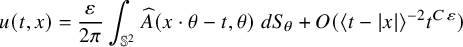 $$ \begin{align}\begin{aligned} u(t,x)&=\frac{\varepsilon}{2\pi}\int_{\mathbb{S}^2}\widehat{ A }(x\cdot\theta-t,\theta)\ dS_\theta+O(\langle t-|x| \rangle^{-2}t^{C\varepsilon}) \end{aligned}\end{align} $$
whenever $t\geq e^{\delta /\varepsilon }$
and
$t\geq e^{\delta /\varepsilon }$
and $|x|<t$
.Footnote
1
Here,
$|x|<t$
.Footnote
1
Here, $\delta \in (0,1)$
is a fixed parameter, and
$\delta \in (0,1)$
is a fixed parameter, and $\widehat { A }=\widehat { A }(q,\omega )$
Footnote
2
is the scattering data obtained from the asymptotic completeness result in [Reference Yu75]. We refer to Section 1.2.3 for the definition of
$\widehat { A }=\widehat { A }(q,\omega )$
Footnote
2
is the scattering data obtained from the asymptotic completeness result in [Reference Yu75]. We refer to Section 1.2.3 for the definition of $\widehat { A }$
. Here, one can view
$\widehat { A }$
. Here, one can view $\widehat { A }$
as a nonlinear version of the Friedlander radiation field for
$\widehat { A }$
as a nonlinear version of the Friedlander radiation field for $\partial u$
.
$\partial u$
.
As a corollary of (1.3), if the equation (1.1) violates the null condition,Footnote
3
then the scattering data $\widehat { A }(q,\omega )$
of a nonzero global solution u to (1.1) and (1.2) cannot decay arbitrarily fast in all directions (i.e., for all
$\widehat { A }(q,\omega )$
of a nonzero global solution u to (1.1) and (1.2) cannot decay arbitrarily fast in all directions (i.e., for all $\omega \in \mathbb {S}^2$
) as
$\omega \in \mathbb {S}^2$
) as $q\to -\infty $
(see Footnote 2). In this paper, we will prove that if the null condition is violated, then the only global solution u to (1.1) and (1.2) satisfying
$q\to -\infty $
(see Footnote 2). In this paper, we will prove that if the null condition is violated, then the only global solution u to (1.1) and (1.2) satisfying
 $$ \begin{align}\begin{aligned} |\widehat{ A }(q,\omega)|\lesssim \langle q \rangle^{-1-},\qquad \forall(q,\omega)\in\mathbb{R}\times\mathbb{S}^2 \end{aligned}\end{align} $$
is the zero solution as long as $\varepsilon \ll 1$
. One can also obtain similar results for the pointwise decay rates of u and
$\varepsilon \ll 1$
. One can also obtain similar results for the pointwise decay rates of u and $\partial u$
. For example, assuming that
$\partial u$
. For example, assuming that
 $$ \begin{align*} |(u_t-u_r)(t,(t-t^{1/2})\omega)|\lesssim \varepsilon t^{-3/2-},\qquad \forall t\geq 1,\ \omega\in\mathbb{S}^2, \end{align*} $$
we have (1.4). As a result, if the null condition is violated, under the pointwise bound for $\partial u$
above, we have
$\partial u$
above, we have $u\equiv 0$
as long as
$u\equiv 0$
as long as $\varepsilon \ll 1$
. We refer to Theorems 2 and 3 for the precise statements of these results.
$\varepsilon \ll 1$
. We refer to Theorems 2 and 3 for the precise statements of these results.
1.1 Background
Let us consider a generalization of the equation (1.1) in $\mathbb {R}^{1+3}$
 $$ \begin{align} \square u^I=F^I(u,\partial u,\partial^2u),\qquad I=1,2,\dots,M. \end{align} $$
The nonlinear terms are assumed to be smooth with the Taylor expansions
 $$ \begin{align}F^I(u,\partial u,\partial^2u)=\sum a_{\alpha\beta,JK}^I\partial^\alpha u^J\partial^\beta u^K+O(|u|^3+|\partial u|^3+|\partial^2 u|^3).\end{align} $$
The sum is taken over all $1\leq J,K\leq M$
and all multiindices
$1\leq J,K\leq M$
and all multiindices $\alpha ,\beta $
with
$\alpha ,\beta $
with $|\alpha |\leq |\beta |\leq 2$
,
$|\alpha |\leq |\beta |\leq 2$
, $|\beta |\geq 1$
and
$|\beta |\geq 1$
and $|\alpha |+|\beta |\leq 3$
. Besides, the coefficients
$|\alpha |+|\beta |\leq 3$
. Besides, the coefficients $a_{\alpha \beta ,JK}^I$
’s are all universal constants.
$a_{\alpha \beta ,JK}^I$
’s are all universal constants.
There have been several results on the lifespans of solutions to the Cauchy problem (1.5) with $C_c^\infty $
initial data of size
$C_c^\infty $
initial data of size $\varepsilon \ll 1$
. For example, John [Reference John29, Reference John28] proved that (1.5) does not necessarily have a global solution. There he proved finite time blowup results for
$\varepsilon \ll 1$
. For example, John [Reference John29, Reference John28] proved that (1.5) does not necessarily have a global solution. There he proved finite time blowup results for $\Box u=u_t^2$
and
$\Box u=u_t^2$
and $\Box u=u_tu_{tt}$
. We also refer to [Reference Alinhac1, Reference Speck68, Reference Holzegel, Klainerman, Speck and Wong23, Reference Christodoulou12, Reference Speck70, Reference Miao and Yu60, Reference Speck69] for the blowup mechanisms for several quasilinear wave equations. For arbitrary nonlinearities, we expect to have almost global existence: the solution exists for all
$\Box u=u_tu_{tt}$
. We also refer to [Reference Alinhac1, Reference Speck68, Reference Holzegel, Klainerman, Speck and Wong23, Reference Christodoulou12, Reference Speck70, Reference Miao and Yu60, Reference Speck69] for the blowup mechanisms for several quasilinear wave equations. For arbitrary nonlinearities, we expect to have almost global existence: the solution exists for all $t\in [0,e^{c/\varepsilon }]$
where
$t\in [0,e^{c/\varepsilon }]$
where $c>0$
is a small constant. We refer to [Reference Lindblad43, Reference John and Klainerman30, Reference Klainerman40, Reference Hörmander24, Reference Hörmander26, Reference Keel, Smith and Sogge36, Reference Keel, Smith and Sogge35] for several cases where this expectation holds, but we remark that it has not been proved for the most general system (1.5); see the discussions in [Reference Metcalfe and Rhoads58, Reference Metcalfe and Morgan56].
$c>0$
is a small constant. We refer to [Reference Lindblad43, Reference John and Klainerman30, Reference Klainerman40, Reference Hörmander24, Reference Hörmander26, Reference Keel, Smith and Sogge36, Reference Keel, Smith and Sogge35] for several cases where this expectation holds, but we remark that it has not been proved for the most general system (1.5); see the discussions in [Reference Metcalfe and Rhoads58, Reference Metcalfe and Morgan56].
To obtain global existence, one needs extra assumptions on the system (1.5). It was proved by Klainerman [Reference Klainerman41, Reference Klainerman39] and Christodoulou [Reference Christodoulou11] that the null condition is sufficient for global existence. We say that (1.5) satisfies the null condition if for each $1\leq I,J,K\leq M$
and for each
$1\leq I,J,K\leq M$
and for each $0\leq m\leq n\leq 2$
with
$0\leq m\leq n\leq 2$
with $n\geq 1$
and
$n\geq 1$
and $m+n\leq 3$
, we have
$m+n\leq 3$
, we have
 $$ \begin{align}\begin{aligned} A_{mn,JK}^I(\omega):=\sum_{|\alpha|=m,|\beta|=n}a_{\alpha\beta,JK}^I\widehat{\omega}^{\alpha}\widehat{\omega}^{\beta}=0,\qquad\text{whenever }\widehat{\omega}=(-1,\omega)\in\mathbb{R}\times\mathbb{S}^2. \end{aligned}\end{align} $$
We also refer to [Reference Sogge67, Reference Metcalfe, Nakamura and Sogge57, Reference Sideris and Tu65] and the references therein for extensions of this global existence result to systems of nonlinear wave equations with multiple wave speeds.
The null condition is not necessary for global existence. In [Reference Lindblad45, Reference Lindblad and Rodnianski48], two examples that violate the null condition in general but admit global existence were presented. One example is the scalar equation (1.1), and the other is the Einstein vacuum equations in wave coordinates. These examples instead satisfy the weak null condition introduced in [Reference Lindblad and Rodnianski47]. Note that the null condition implies the weak null condition and that both $\Box u=u_t^2$
and
$\Box u=u_t^2$
and $\Box u=u_tu_{tt}$
violate the weak null condition. There is a conjecture that the weak null condition is sufficient for global existence,Footnote
4
and we refer to [Reference Keir37, Reference Keir38, Reference Kadar32] for recent progress on it.
$\Box u=u_tu_{tt}$
violate the weak null condition. There is a conjecture that the weak null condition is sufficient for global existence,Footnote
4
and we refer to [Reference Keir37, Reference Keir38, Reference Kadar32] for recent progress on it.
To define the weak null condition, we introduce a type of asymptotic equations derived by Hörmander [Reference Hörmander24, Reference Hörmander25, Reference Hörmander26]. Suppose that u is a global solution to (1.5) and we make the ansatz
 $$ \begin{align} u^I(t,x)\approx \varepsilon r^{-1}U^I(s,q,\omega),\hspace{1cm}r=|x|,\ \omega=x/r,\ s=\varepsilon\ln t,\ q=r-t,\ 1\leq I\leq M. \end{align} $$
Assuming that $t=r\to \infty $
, we substitute this ansatz into (1.5) and compare the coefficients of terms of order
$t=r\to \infty $
, we substitute this ansatz into (1.5) and compare the coefficients of terms of order $\varepsilon ^2 t^{-2}$
. We thus obtain the following asymptotic PDE’s (called Hörmander’s asymptotic equations for (1.5)) for
$\varepsilon ^2 t^{-2}$
. We thus obtain the following asymptotic PDE’s (called Hörmander’s asymptotic equations for (1.5)) for $U=(U^{I}(s,q,\omega ))$
:
$U=(U^{I}(s,q,\omega ))$
:
 $$ \begin{align}2\partial_s\partial_q U^I=\sum A_{mn,JK}^I(\omega)\partial_q^mU^J\partial_q^nU^K.\end{align} $$
Here, $A_{mn,JK}^I$
is defined by (1.7), and the sum in (1.9) is taken over
$A_{mn,JK}^I$
is defined by (1.7), and the sum in (1.9) is taken over $0\leq m\leq n\leq 2$
with
$0\leq m\leq n\leq 2$
with $n\geq 1$
and
$n\geq 1$
and $m+n\leq 3$
. We say that (1.5) satisfies the weak null condition if the corresponding (1.9) has a global solution for all
$m+n\leq 3$
. We say that (1.5) satisfies the weak null condition if the corresponding (1.9) has a global solution for all $s\geq 0$
and if the solution and all its derivatives grow at most exponentially in s, provided that the initial data decay sufficiently fast in q. For example, for the scalar equation (1.1), the corresponding asymptotic equation (1.9) becomes
$s\geq 0$
and if the solution and all its derivatives grow at most exponentially in s, provided that the initial data decay sufficiently fast in q. For example, for the scalar equation (1.1), the corresponding asymptotic equation (1.9) becomes
 $$ \begin{align}2\partial_s\partial_q U=G(\omega)U\partial_q^2U,\end{align} $$
where
 $$ \begin{align}\begin{aligned} G(\omega):=g_0^{\alpha\beta}\widehat{\omega}_\alpha\widehat{\omega}_\beta,\qquad g_0^{\alpha\beta}=\frac{d}{du}g^{\alpha\beta}(u)|_{u=0},\ \widehat{\omega}=(-1,\omega)\in\mathbb{R}\times\mathbb{S}^2. \end{aligned}\end{align} $$
One can prove the global existence and growth control for (1.10), so (1.1) satisfies the weak null condition.
1.2 The modified scattering for (1.1)
Following the global existence result in [Reference Lindblad45], we are interested in the long time dynamics for the equation (1.1). Recently, the modified scattering for (1.1) was established. In this subsection, we give an overview of the results in [Reference Yu75, Reference Yu73, Reference Yu72] and discuss some related works on the long time dynamics for general quasilinear wave equations in $\mathbb {R}^{1+3}$
.
$\mathbb {R}^{1+3}$
.
1.2.1 The geometric reduced system
Instead of Hörmander’s asymptotic equation (1.10), we used a new system of asymptotic equations for (1.1) to study its long time dynamics in [Reference Yu75, Reference Yu73, Reference Yu72]. It is called the geometric reduced system, and it is expected to describe the asymptotic behaviors of global solutions to (1.1) more accurately than (1.10) does.
To derive the geometric reduced system, we return to the ansatz (1.8) (with $M=1$
) used in the derivation of (1.10). We still make the ansatz
$M=1$
) used in the derivation of (1.10). We still make the ansatz
 $$ \begin{align}\begin{aligned} u(t,x)\approx \varepsilon r^{-1}U(s,q,\omega),\qquad r=|x|,\ \omega=x/r,\ s=\varepsilon\ln t, \end{aligned}\end{align} $$
but now we let $q(t,x)$
be an optical function that is close to
$q(t,x)$
be an optical function that is close to $r-t$
to some extent. By an optical function, we mean that q solves the eikonal equation
$r-t$
to some extent. By an optical function, we mean that q solves the eikonal equation
 $$ \begin{align}\begin{aligned} g^{\alpha\beta}(u)\partial_\alpha q\partial_\beta q=0. \end{aligned}\end{align} $$
Eikonal equations have been widely used in the study of nonlinear wave equations and the Einstein equations; see, for example, [Reference Alinhac2, Reference Lindblad45, Reference Christodoulou and Klainerman13, Reference Lindblad46, Reference Smith and Tataru66, Reference Klainerman, Rodnianski and Szeftel42, Reference Keir37]. Our new ansatz is related to the geometry of the null cone with respect to the Lorentzian metric $(g_{\alpha \beta })$
that is the inverse of the
$(g_{\alpha \beta })$
that is the inverse of the $4\times 4$
matrix
$4\times 4$
matrix $(g^{\alpha \beta }(u))$
. Since the geometric information from (1.1) is considered in our derivation, we expect to obtain a more accurate type of asymptotic equations for (1.1).
$(g^{\alpha \beta }(u))$
. Since the geometric information from (1.1) is considered in our derivation, we expect to obtain a more accurate type of asymptotic equations for (1.1).
When substituting the ansatz above into (1.1), we obtain an equation involving $\partial q$
. However, the optical function has no explicit formula because the eikonal equation is fully nonlinear. Alternatively, we define an auxiliary function
$\partial q$
. However, the optical function has no explicit formula because the eikonal equation is fully nonlinear. Alternatively, we define an auxiliary function $\mu =q_t-q_r$
and express
$\mu =q_t-q_r$
and express $\partial q$
approximately in terms of
$\partial q$
approximately in terms of $\mu $
and U using the eikonal equation. By sending
$\mu $
and U using the eikonal equation. By sending $t=r\to \infty $
and considering terms of order
$t=r\to \infty $
and considering terms of order $\varepsilon ^2t^{-2}$
in (1.1), we obtain the following reduced system for
$\varepsilon ^2t^{-2}$
in (1.1), we obtain the following reduced system for $(\mu ,U)(s,q,\omega )$
:
$(\mu ,U)(s,q,\omega )$
:
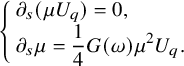 $$ \begin{align}\begin{aligned} \left\{\begin{array}{l} \displaystyle \partial_s (\mu U_q)=0,\\ \displaystyle \partial_s\mu=\frac{1}{4}G(\omega)\mu^2U_q.\end{array}\right. \end{aligned}\end{align} $$
Here, $G(\omega )$
is defined by (1.11). The system (1.14) is the geometric reduced system for (1.1). By setting
$G(\omega )$
is defined by (1.11). The system (1.14) is the geometric reduced system for (1.1). By setting $(\mu ,U_q)|_{s=0}(q,\omega )=(A_1,A_2)(q,\omega )$
, we obtain an explicit solution to (1.14):
$(\mu ,U_q)|_{s=0}(q,\omega )=(A_1,A_2)(q,\omega )$
, we obtain an explicit solution to (1.14):
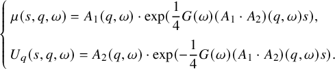 $$ \begin{align}\begin{aligned} \left\{\begin{array}{l}\displaystyle \mu(s,q,\omega)=A_1(q,\omega)\cdot \exp(\frac{1}{4}G(\omega)(A_1\cdot A_2)(q,\omega)s),\\[1em] \displaystyle U_q(s,q,\omega)=A_2(q,\omega)\cdot \exp(-\frac{1}{4}G(\omega)(A_1\cdot A_2)(q,\omega)s).\end{array}\right. \end{aligned}\end{align} $$
In fact, the first equation in (1.14) yields $\mu U_q=A_1A_2$
for all
$\mu U_q=A_1A_2$
for all $s\geq 0$
, so the second equation in (1.14) is reduced to a linear ODE. From this perspective, the reduced system (1.14) is of a simpler form than (1.10), which is a nonlinear PDE.
$s\geq 0$
, so the second equation in (1.14) is reduced to a linear ODE. From this perspective, the reduced system (1.14) is of a simpler form than (1.10), which is a nonlinear PDE.
We finally remark that the derivation above can be extended. Given an arbitrary system of quasilinear wave equations in $\mathbb {R}^{1+3}$
, we can derive the corresponding geometric reduced system. See [Reference Yu72, Chapter 2] and [Reference Yu74, (1.11)].
$\mathbb {R}^{1+3}$
, we can derive the corresponding geometric reduced system. See [Reference Yu72, Chapter 2] and [Reference Yu74, (1.11)].
1.2.2 Existence of modified wave operators
Making use of (1.14), we proved the existence of the modified wave operators for (1.1) in [Reference Yu73]. Given an asymptotic profile, we seek to find a global solution to (1.1) such that this global solution matches the given asymptotic profile at infinite time. Such a problem is sometimes referred to as a backward scattering problem. To the best of the author’s knowledge, [Reference Yu73] seems to be the only result on the modified wave operators for (1.1). We refer to Lindblad-Schlue [Reference Lindblad and Schlue50, Reference Lindblad and Schlue49] for backward scattering for semilinear wave equations satisfying the null condition or the weak null condition and some related models. Also see [Reference Dafermos, Holzegel and Rodnianski14, Reference Chen and Lindblad10, Reference He22, Reference Chen9, Reference Kadar31, Reference Ionescu and Pausader27, Reference Ouyang61] and the references therein for similar results for the Einstein equations and other wave-type models.
Let us specify how the asymptotic profile is chosen in [Reference Yu73]. Fix an arbitrary $A(q,\omega )\in C_c^\infty (\mathbb {R}\times \mathbb {S}^2)$
and suppose that
$A(q,\omega )\in C_c^\infty (\mathbb {R}\times \mathbb {S}^2)$
and suppose that $\operatorname {\mathrm {supp}} A\subset [-R,R]\times \mathbb {S}^2$
for some constant
$\operatorname {\mathrm {supp}} A\subset [-R,R]\times \mathbb {S}^2$
for some constant $R>0$
. Define
$R>0$
. Define $(\mu ,U_q)(s,q,\omega )$
by (1.15) with
$(\mu ,U_q)(s,q,\omega )$
by (1.15) with $(A_1,A_2)=(-2,A)$
.Footnote
5
That is, we set
$(A_1,A_2)=(-2,A)$
.Footnote
5
That is, we set
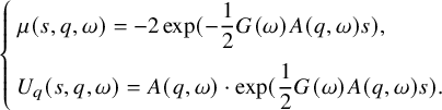 $$ \begin{align}\begin{aligned} \left\{\begin{array}{l}\displaystyle \mu(s,q,\omega)=-2\exp(-\frac{1}{2}G(\omega)A(q,\omega)s),\\[1em] \displaystyle U_q(s,q,\omega)=A(q,\omega)\cdot \exp(\frac{1}{2}G(\omega)A(q,\omega)s).\end{array}\right. \end{aligned}\end{align} $$
We call this A the scattering data for the modified wave operator problem. To uniquely determine U, we add a boundary condition $\lim _{q\to -\infty }U(s,q,\omega )=0$
.Footnote
6
As a result, we obtain a solution
$\lim _{q\to -\infty }U(s,q,\omega )=0$
.Footnote
6
As a result, we obtain a solution $(\mu ,U)(s,q,\omega )$
to the geometric reduced system (1.14) for all
$(\mu ,U)(s,q,\omega )$
to the geometric reduced system (1.14) for all $s\geq 0$
.
$s\geq 0$
.
We now fix $\delta \in (0,1)$
which corresponds to the initial time when our reduced system starts to play a roleFootnote
7
and
$\delta \in (0,1)$
which corresponds to the initial time when our reduced system starts to play a roleFootnote
7
and $\varepsilon \ll 1$
, which is the size of the global solution we will construct. We recover an approximate optical function
$\varepsilon \ll 1$
, which is the size of the global solution we will construct. We recover an approximate optical function $q(t,x)$
by solving the transport equation introduced in the derivation of (1.14)
$q(t,x)$
by solving the transport equation introduced in the derivation of (1.14)
 $$ \begin{align*} (q_t-q_r)(t,x)=\mu(\varepsilon\ln t-\delta,q(t,x),x/|x|). \end{align*} $$
We choose the boundary condition so that $q\approx r-t$
to some extent. Motivated by the new ansatz (1.12), we define
$q\approx r-t$
to some extent. Motivated by the new ansatz (1.12), we define
 $$ \begin{align}\begin{aligned} \varepsilon |x|^{-1}U(\varepsilon\ln t-\delta,q(t,x),x/|x|) \end{aligned}\end{align} $$
as the asymptotic profile in this problem. One can show that (1.17) is an approximate solution to (1.1) whenever $|r-t|<t/2$
and
$|r-t|<t/2$
and $t>e^{\delta /\varepsilon }$
. In [Reference Yu73], we proved that there exists a global solution u to (1.1) for all
$t>e^{\delta /\varepsilon }$
. In [Reference Yu73], we proved that there exists a global solution u to (1.1) for all $t\geq 0$
such that u matches the asymptotic profile (1.17) at infinite time. See [Reference Yu73, Theorem 1]. For example, we have
$t\geq 0$
such that u matches the asymptotic profile (1.17) at infinite time. See [Reference Yu73, Theorem 1]. For example, we have
 $$ \begin{align}\begin{aligned} |u-\varepsilon r^{-1}U|\lesssim \varepsilon t^{-3/2+C\varepsilon}\langle r-t \rangle^{1/2} \end{aligned}\end{align} $$
for all $t\gtrsim 1$
and
$t\gtrsim 1$
and $|x|\leq 5t/4$
. Note that
$|x|\leq 5t/4$
. Note that $u|_{|x|\leq t- R}\equiv 0$
and
$u|_{|x|\leq t- R}\equiv 0$
and $U|_{q\leq -R}\equiv 0$
, so the estimate (1.18) is trivial for
$U|_{q\leq -R}\equiv 0$
, so the estimate (1.18) is trivial for $|x|\leq t-R$
. Recall that the constant R comes from the support of A. By comparing (1.18) with the pointwise decay
$|x|\leq t-R$
. Recall that the constant R comes from the support of A. By comparing (1.18) with the pointwise decay $u=O(\varepsilon t^{-1+C\varepsilon })$
, we conclude that the asymptotic profile (1.17) approximates the global solution u well whenever
$u=O(\varepsilon t^{-1+C\varepsilon })$
, we conclude that the asymptotic profile (1.17) approximates the global solution u well whenever $|r-t|\lesssim t^{1-}$
.
$|r-t|\lesssim t^{1-}$
.
In a recent work [Reference Yu74], the main theorem in [Reference Yu73] was extended in two different ways. First, the assumption $A\in C_c^\infty $
is relaxed. To prove the existence of the modified wave operators for (1.1), we only need to assume that
$A\in C_c^\infty $
is relaxed. To prove the existence of the modified wave operators for (1.1), we only need to assume that $A\in C^\infty $
and that
$A\in C^\infty $
and that
 $$ \begin{align}\begin{aligned} |\partial_q^a\partial_\omega^cA(q,\omega)|&\lesssim_{a,c} \langle q \rangle^{-\gamma_--a}\cdot 1_{q<0}+\langle q \rangle^{-\gamma_+-a}\cdot 1_{q\geq 0},\qquad \forall (q,\omega)\in\mathbb{R}\times\mathbb{S}^2,\ a,c\geq 0 \end{aligned}\end{align} $$
where $\gamma _->2$
and
$\gamma _->2$
and $\gamma _+>1$
are two fixed parameters. See [Reference Yu74, Corollary 8.1]. Moreover, the method in [Reference Yu73] can be applied to a larger class of quasilinear wave equations in three space dimensions. In particular, one obtains nontrivial global solutions to
$\gamma _+>1$
are two fixed parameters. See [Reference Yu74, Corollary 8.1]. Moreover, the method in [Reference Yu73] can be applied to a larger class of quasilinear wave equations in three space dimensions. In particular, one obtains nontrivial global solutions to $\Box u=u_t^2$
and
$\Box u=u_t^2$
and $\Box u=u_tu_{tt}$
for all
$\Box u=u_tu_{tt}$
for all $t\geq 0$
, despite the finite time blowup results by John. See [Reference Yu74, Corollaries 8.3 and 8.9].
$t\geq 0$
, despite the finite time blowup results by John. See [Reference Yu74, Corollaries 8.3 and 8.9].
1.2.3 Asymptotic completeness
In [Reference Yu75], we proved the asymptotic completeness for (1.1). Given a global solution to (1.1) with initial data (1.2), we seek to find the corresponding asymptotic profile. Before [Reference Yu75], Deng and Pusateri [Reference Deng and Pusateri17] proved a partial scattering result for (1.1) using Hörmander’s asymptotic equation (1.10). They applied the spacetime resonance method, and we refer to [Reference Pusateri and Shatah64, Reference Pusateri63] for some earlier applications of this method. We also refer to [Reference Lindblad46, Reference Chen9, Reference Chen and Lindblad10, Reference Candy, Kauffman and Lindblad8, Reference Katayama33, Reference Katayama and Kubo34, Reference Ionescu and Pausader27] and the references therein for similar results for the Einstein equations and other wave-type models.
We now briefly explain the proof. More details are provided in Section 3 below. Suppose that u is the global solution to (1.1) with data (1.2) of size $\varepsilon \ll 1$
. Let
$\varepsilon \ll 1$
. Let $R>0$
be a constant such that
$R>0$
be a constant such that $\operatorname {\mathrm {supp}}(u_0,u_1)\subset \{|x|\leq R\}$
. We first construct a global optical function
$\operatorname {\mathrm {supp}}(u_0,u_1)\subset \{|x|\leq R\}$
. We first construct a global optical function $q(t,x)$
by solving the eikonal equation (1.13) for all
$q(t,x)$
by solving the eikonal equation (1.13) for all $|x|>t/2$
and
$|x|>t/2$
and $t>e^{\delta /\varepsilon }$
where
$t>e^{\delta /\varepsilon }$
where $\delta \in (0,1)$
is a small fixed parameter.Footnote
8
The boundary condition is chosen so that
$\delta \in (0,1)$
is a small fixed parameter.Footnote
8
The boundary condition is chosen so that $q\approx r-t$
. In the proof, we apply both the method of characteristics and the method from [Reference Christodoulou and Klainerman13, Reference Smith and Tataru66]. The key step is to carefully estimate the second fundamental form
$q\approx r-t$
. In the proof, we apply both the method of characteristics and the method from [Reference Christodoulou and Klainerman13, Reference Smith and Tataru66]. The key step is to carefully estimate the second fundamental form $(\chi _{ab})_{a,b=1,2}$
with the help of the Raychaudhuri equation.
$(\chi _{ab})_{a,b=1,2}$
with the help of the Raychaudhuri equation.
Next, motivated by the ansatz (1.12), we define $(\mu ,U):=(q_t-q_r,\varepsilon ^{-1}ru)$
. Both
$(\mu ,U):=(q_t-q_r,\varepsilon ^{-1}ru)$
. Both $\mu $
and U are originally functions of
$\mu $
and U are originally functions of $(t,x)$
for
$(t,x)$
for $|x|>t/2$
and
$|x|>t/2$
and $t>e^{\delta /\varepsilon }$
, and can be viewed as functions of
$t>e^{\delta /\varepsilon }$
, and can be viewed as functions of $(s,q,\omega )$
via the inverse of the map
$(s,q,\omega )$
via the inverse of the map
 $$ \begin{align*} (t,x)\mapsto(\varepsilon\ln t-\delta,q(t,x),x/|x|)=(s,q,\omega). \end{align*} $$
This $(\mu ,U)(s,q,\omega )$
is an approximate solution to the geometric reduced system (1.14), and there is an exact solution
$(\mu ,U)(s,q,\omega )$
is an approximate solution to the geometric reduced system (1.14), and there is an exact solution $(\widetilde { \mu },\widetilde { U })(s,q,\omega )$
Footnote
9
to (1.14) matching
$(\widetilde { \mu },\widetilde { U })(s,q,\omega )$
Footnote
9
to (1.14) matching $(\mu ,U)(s,q,\omega )$
at infinite time; see (3.5) and (3.6) below. Following the discussion in Section 1.2.2, we hope that
$(\mu ,U)(s,q,\omega )$
at infinite time; see (3.5) and (3.6) below. Following the discussion in Section 1.2.2, we hope that $(\widetilde { \mu },\widetilde { U })$
is also of the form (1.16), so we can define the scattering data as the initial data of
$(\widetilde { \mu },\widetilde { U })$
is also of the form (1.16), so we can define the scattering data as the initial data of $\widetilde { U }_q$
at
$\widetilde { U }_q$
at $s=0$
. However, this is impossible since we may have
$s=0$
. However, this is impossible since we may have $\widetilde { \mu }|_{s=0}\not \equiv -2$
. To handle this issue, we use the gauge freedom (see Footnote 5) to transform
$\widetilde { \mu }|_{s=0}\not \equiv -2$
. To handle this issue, we use the gauge freedom (see Footnote 5) to transform $(\widetilde { \mu },\widetilde { U })$
to an equivalent exact solution
$(\widetilde { \mu },\widetilde { U })$
to an equivalent exact solution $(\widehat { \mu },\widehat { U })$
to (1.14) with
$(\widehat { \mu },\widehat { U })$
to (1.14) with $\widehat { \mu }|_{s=0}\equiv -2$
; see (3.15) and (3.16) below. This new solution
$\widehat { \mu }|_{s=0}\equiv -2$
; see (3.15) and (3.16) below. This new solution $(\widehat { \mu },\widehat { U })$
is of the form (1.16) with A replaced by
$(\widehat { \mu },\widehat { U })$
is of the form (1.16) with A replaced by $\widehat { A }=\widehat { U }_q|_{s=0}$
. This function
$\widehat { A }=\widehat { U }_q|_{s=0}$
. This function $\widehat { A }$
is called the scattering data in the asymptotic completeness problemFootnote
10
and will play the same role as the scattering data A in the modified wave operator problem. In general, one cannot show that
$\widehat { A }$
is called the scattering data in the asymptotic completeness problemFootnote
10
and will play the same role as the scattering data A in the modified wave operator problem. In general, one cannot show that $\widehat { A }$
is
$\widehat { A }$
is $C^\infty $
. Instead, for each integer
$C^\infty $
. Instead, for each integer $N\geq 0$
, there exists an
$N\geq 0$
, there exists an $\varepsilon _N>0$
depending on N, such that for all
$\varepsilon _N>0$
depending on N, such that for all $\varepsilon \in (0,\varepsilon _N)$
,Footnote
11
we have
$\varepsilon \in (0,\varepsilon _N)$
,Footnote
11
we have $\widehat { A }\in C^N$
and
$\widehat { A }\in C^N$
and
 $$ \begin{align}\begin{aligned} |\partial_q^a\partial_\omega^c\widehat{ A }(q,\omega)|&\lesssim_{a,c} \langle q \rangle^{-1-a+C_{a,c}\varepsilon},\qquad \forall (q,\omega)\in\mathbb{R}\times\mathbb{S}^2,\ a,c\geq 0,\ a+c\leq N. \end{aligned}\end{align} $$
The constants $C_{a,c}$
and the implicit constants in
$C_{a,c}$
and the implicit constants in $\lesssim _{a,c}$
are all uniform in
$\lesssim _{a,c}$
are all uniform in $\varepsilon $
. We also show a gauge independence result: for each fixed parameter
$\varepsilon $
. We also show a gauge independence result: for each fixed parameter $\delta $
, the scattering data
$\delta $
, the scattering data $\widehat { A }$
is independent of the choice of the optical function; see Corollary 3.9.
$\widehat { A }$
is independent of the choice of the optical function; see Corollary 3.9.
Finally, we construct an approximate solution $\widetilde { u }$
to (1.1) from
$\widetilde { u }$
to (1.1) from $(\widetilde { \mu },\widetilde { U })$
Footnote
12
by following the construction in [Reference Yu73, Section 4]. That is, we construct an approximate optical function
$(\widetilde { \mu },\widetilde { U })$
Footnote
12
by following the construction in [Reference Yu73, Section 4]. That is, we construct an approximate optical function $\widetilde { q }$
by solving
$\widetilde { q }$
by solving $\widetilde { q }_t-\widetilde { q }_r=\widetilde { \mu }$
, and define
$\widetilde { q }_t-\widetilde { q }_r=\widetilde { \mu }$
, and define $\widetilde { u }$
by (1.17) with
$\widetilde { u }$
by (1.17) with $(U,q)$
replaced by
$(U,q)$
replaced by $(\widetilde { U },\widetilde { q })$
. Then,
$(\widetilde { U },\widetilde { q })$
. Then, $\widetilde { u }$
is an approximate solution to (1.1) for
$\widetilde { u }$
is an approximate solution to (1.1) for $|x|>t/2$
and
$|x|>t/2$
and $t>e^{\delta /\varepsilon }$
. In addition, we prove that
$t>e^{\delta /\varepsilon }$
. In addition, we prove that $\widetilde { u }$
offers a good approximation of u at least near the light cone. See [Reference Yu75, Theorem 1] for a precise statement. For example, we have
$\widetilde { u }$
offers a good approximation of u at least near the light cone. See [Reference Yu75, Theorem 1] for a precise statement. For example, we have
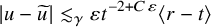 $$ \begin{align}\begin{aligned} |u-\widetilde{ u }|\lesssim_\gamma \varepsilon t^{-2+C\varepsilon}\langle r-t \rangle \end{aligned}\end{align} $$
whenever $t>e^{\delta /\varepsilon }$
and
$t>e^{\delta /\varepsilon }$
and $|x|\geq t-t^\gamma $
, where
$|x|\geq t-t^\gamma $
, where $\gamma \in (0,1)$
is a fixed parameter. Note that
$\gamma \in (0,1)$
is a fixed parameter. Note that $u\equiv \widetilde { u }\equiv 0$
whenever
$u\equiv \widetilde { u }\equiv 0$
whenever $|x|\geq t+R$
by the finite speed of propagation, so the estimate (1.21) is trivial for
$|x|\geq t+R$
by the finite speed of propagation, so the estimate (1.21) is trivial for $|x|\geq t+R$
. Recall that the constant R comes from the support of the initial data (1.2).
$|x|\geq t+R$
. Recall that the constant R comes from the support of the initial data (1.2).
1.2.4 More about the long time dynamics
From [Reference Yu75, Reference Yu72, Reference Yu73, Reference Yu74], one may contend that the asymptotic behaviors of global solutions to (1.1) have been fully understood. This is, however, not true. For example, the following question is not answered in these papers.
Question 1.1. In both the modified wave operator problem and the asymptotic completeness problem, can we give a full description of the asymptotic behaviors of the global solutions to (1.1)?
In the modified wave operator problem, starting from a scattering data A, we construct an asymptotic profile (1.17) and find the matching global solution u to (1.1). The estimate (1.18) suggests that $u\approx \varepsilon r^{-1}U$
for
$u\approx \varepsilon r^{-1}U$
for $t\gg 1$
and
$t\gg 1$
and $r\leq t+t^{1-}$
. However, we do not have a good way to describe the asymptotic behaviors of u outside the light cone. From [Reference Yu74, Reference Yu73], we only know that
$r\leq t+t^{1-}$
. However, we do not have a good way to describe the asymptotic behaviors of u outside the light cone. From [Reference Yu74, Reference Yu73], we only know that $|u|\lesssim \varepsilon t^{-1/2+C\varepsilon }r^{-1/2}$
whenever
$|u|\lesssim \varepsilon t^{-1/2+C\varepsilon }r^{-1/2}$
whenever $t\gg 1$
and
$t\gg 1$
and $r\geq 5t/4$
.
$r\geq 5t/4$
.
A similar issue arises in the forward problem. Let u be the global solution to the Cauchy problem (1.1) and (1.2). In the asymptotic completeness problem, we find the scattering data $\widehat { A }$
and define an approximate solution
$\widehat { A }$
and define an approximate solution $\widetilde { u }$
to (1.1). The estimate (1.21) suggests that
$\widetilde { u }$
to (1.1). The estimate (1.21) suggests that $u\approx \widetilde { u }$
for
$u\approx \widetilde { u }$
for $t\gg _\varepsilon 1$
and
$t\gg _\varepsilon 1$
and $r\geq t-t^{1-}$
. The asymptotic behaviors of u inside the light cone (e.g., for
$r\geq t-t^{1-}$
. The asymptotic behaviors of u inside the light cone (e.g., for $r<t/2$
), however, are not discussed in [Reference Yu75, Reference Deng and Pusateri17]. We only know from [Reference Lindblad45] that
$r<t/2$
), however, are not discussed in [Reference Yu75, Reference Deng and Pusateri17]. We only know from [Reference Lindblad45] that $u=O(\varepsilon t^{-1+C\varepsilon })$
.
$u=O(\varepsilon t^{-1+C\varepsilon })$
.
Question 1.1 arises because of the limitations of Hörmander’s asymptotic equations and geometric reduced systems. Both these asymptotic equations are derived under the assumption that $r=t\to \infty $
, so they are expected to approximate the original wave equations well only at null infinity. It is thus necessary to find a different way to describe the asymptotic behaviors of global solutions away from the light cone.
$r=t\to \infty $
, so they are expected to approximate the original wave equations well only at null infinity. It is thus necessary to find a different way to describe the asymptotic behaviors of global solutions away from the light cone.
We now discuss some previous results related to Question 1.1. For simplicity, our discussions will be restricted to the wave equations (e.g., (1.5)) in $\mathbb {R}^{1+3}$
. For the backward problem, Lindblad and Schlue [Reference Lindblad and Schlue49] constructed a global solution to
$\mathbb {R}^{1+3}$
. For the backward problem, Lindblad and Schlue [Reference Lindblad and Schlue49] constructed a global solution to $\Box u=0$
with prescribed radiation fields. Unlike the results in [Reference Lindblad and Schlue50], in [Reference Lindblad and Schlue49, Theorem 1.5] they gave a complete characterization of the asymptotics of the solution towards timelike and spacelike infinity.
$\Box u=0$
with prescribed radiation fields. Unlike the results in [Reference Lindblad and Schlue50], in [Reference Lindblad and Schlue49, Theorem 1.5] they gave a complete characterization of the asymptotics of the solution towards timelike and spacelike infinity.
In the forward problem, we first recall the strong Huygens principle: a solution to $\Box u=0$
with compactly supported data must vanish for
$\Box u=0$
with compactly supported data must vanish for $|r-t|\gtrsim 1$
. This principle is, however, unstable [Reference Günther21, Reference Mathisson55]. A related result is Price’s law, which was first conjectured in [Reference Price62]. It states that we have a
$|r-t|\gtrsim 1$
. This principle is, however, unstable [Reference Günther21, Reference Mathisson55]. A related result is Price’s law, which was first conjectured in [Reference Price62]. It states that we have a $t^{-3}$
local uniform decay rate for linear waves on the Schwarzschild background, and we refer to [Reference Dafermos and Rodnianski15, Reference Donninger, Schlag and Soffer19, Reference Donninger, Schlag and Soffer20, Reference Tataru71, Reference Metcalfe, Tataru and Tohaneanu59] for its proof. For a system (1.5) satisfying the null condition along with
$t^{-3}$
local uniform decay rate for linear waves on the Schwarzschild background, and we refer to [Reference Dafermos and Rodnianski15, Reference Donninger, Schlag and Soffer19, Reference Donninger, Schlag and Soffer20, Reference Tataru71, Reference Metcalfe, Tataru and Tohaneanu59] for its proof. For a system (1.5) satisfying the null condition along with $C_c^\infty $
data of size
$C_c^\infty $
data of size $\varepsilon \ll 1$
, Christodoulou [Reference Christodoulou11] obtained a pointwise decay
$\varepsilon \ll 1$
, Christodoulou [Reference Christodoulou11] obtained a pointwise decay $u=O(\varepsilon \langle r-t \rangle ^{-1}\langle r+t \rangle ^{-1})$
. This bound is not optimal for a scalar semilinear or quasilinear wave equation satisfying the null condition with constant-coefficient null forms. In those cases, we have
$u=O(\varepsilon \langle r-t \rangle ^{-1}\langle r+t \rangle ^{-1})$
. This bound is not optimal for a scalar semilinear or quasilinear wave equation satisfying the null condition with constant-coefficient null forms. In those cases, we have $u=O(\varepsilon \langle r-t \rangle ^{-2}\langle r+t \rangle ^{-1})$
; see [Reference Dong, Ma, Ma and Yuan18, Reference Luk and Oh54, Reference Luk and Oh53]. However, if we pose the initial data on a hyperboloid instead of a time slice, and if we do not assume that the data is compactly supported, then the bound
$u=O(\varepsilon \langle r-t \rangle ^{-2}\langle r+t \rangle ^{-1})$
; see [Reference Dong, Ma, Ma and Yuan18, Reference Luk and Oh54, Reference Luk and Oh53]. However, if we pose the initial data on a hyperboloid instead of a time slice, and if we do not assume that the data is compactly supported, then the bound $u=O(\varepsilon \langle r-t \rangle ^{-1}\langle r+t \rangle ^{-1})$
is optimal; see [Reference Dong, Ma, Ma and Yuan18]. A similar result on the sharp pointwise decay for a semilinear wave equation with the null condition in nonstationary and asymptotically flat spacetimes can be found in [Reference Looi and Tohaneanu51]. We also remark that a closely related topic is the late time tail for solutions to wave equations on asymptotically flat spacetimes. In this direction, we refer to, for example, [Reference Luk and Oh54, Reference Angelopoulos, Aretakis and Gajic4, Reference Angelopoulos, Aretakis and Gajic5, Reference Angelopoulos, Aretakis and Gajic6, Reference Angelopoulos, Aretakis and Gajic7, Reference Looi and Xiong52], and the references therein (in particular, see Luk-Oh [Reference Luk and Oh54, Section 1.3]).
$u=O(\varepsilon \langle r-t \rangle ^{-1}\langle r+t \rangle ^{-1})$
is optimal; see [Reference Dong, Ma, Ma and Yuan18]. A similar result on the sharp pointwise decay for a semilinear wave equation with the null condition in nonstationary and asymptotically flat spacetimes can be found in [Reference Looi and Tohaneanu51]. We also remark that a closely related topic is the late time tail for solutions to wave equations on asymptotically flat spacetimes. In this direction, we refer to, for example, [Reference Luk and Oh54, Reference Angelopoulos, Aretakis and Gajic4, Reference Angelopoulos, Aretakis and Gajic5, Reference Angelopoulos, Aretakis and Gajic6, Reference Angelopoulos, Aretakis and Gajic7, Reference Looi and Xiong52], and the references therein (in particular, see Luk-Oh [Reference Luk and Oh54, Section 1.3]).
Our final remark is that all the references listed in the previous two paragraphs do not apply to (1.1). This is due to its weak null structure.
1.3 The main theorems
In this paper, we will partially answer Question 1.1 by providing a description of the asymptotic behaviors of a global solution u to the forward Cauchy problem (1.1) and (1.2) inside the light cone. We will present an asymptotic formula for $Z^Iu$
for each multiindex I. Here, Z denotes one of the commuting vector fields: translations
$Z^Iu$
for each multiindex I. Here, Z denotes one of the commuting vector fields: translations $\partial _\alpha $
, scaling
$\partial _\alpha $
, scaling $S=t\partial _t+r\partial _r$
, rotations
$S=t\partial _t+r\partial _r$
, rotations $\Omega _{ij}=x_i\partial _j-x_j\partial _i$
, and Lorentz boosts
$\Omega _{ij}=x_i\partial _j-x_j\partial _i$
, and Lorentz boosts $\Omega _{0i}=x_i\partial _t+t\partial _i$
. Besides,
$\Omega _{0i}=x_i\partial _t+t\partial _i$
. Besides, $Z^I$
denotes a product of
$Z^I$
denotes a product of $|I|$
commuting vector fields for each multiindex I.
$|I|$
commuting vector fields for each multiindex I.
Fix $(u_0,u_1)\in C_c^\infty (\mathbb {R}^3)$
. From [Reference Lindblad45], we know that the Cauchy problem (1.1) and (1.2) admits a unique global
$(u_0,u_1)\in C_c^\infty (\mathbb {R}^3)$
. From [Reference Lindblad45], we know that the Cauchy problem (1.1) and (1.2) admits a unique global $C^\infty $
solution u for all
$C^\infty $
solution u for all $t\geq 0$
as long as
$t\geq 0$
as long as $\varepsilon \ll 1$
. In Section 1.2.3, for a fixed
$\varepsilon \ll 1$
. In Section 1.2.3, for a fixed $\delta \in (0,1)$
, we explained how to construct the scattering data
$\delta \in (0,1)$
, we explained how to construct the scattering data $\widehat { A }$
for the global solution u. For each multiindex I, we define
$\widehat { A }$
for the global solution u. For each multiindex I, we define $A_I=A_I(q,\omega )$
inductively by
$A_I=A_I(q,\omega )$
inductively by $A_0=-2\widehat { A }$
and
$A_0=-2\widehat { A }$
and
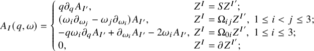 $$ \begin{align}\begin{aligned} A_I(q,\omega)=\left\{ \begin{array}{ll} q\partial_qA_{I'}, & Z^I=SZ^{I'}; \\ (\omega_i\partial_{\omega_j}-\omega_j\partial_{\omega_i})A_{I'}, & Z^I=\Omega_{ij}Z^{I'},\ 1\leq i<j\leq 3;\\ -q\omega_i\partial_qA_{I'}+\partial_{\omega_i}A_{I'}-2\omega_iA_{I'}, & Z^I=\Omega_{0i}Z^{I'},\ 1\leq i\leq 3;\\ 0, & Z^I=\partial Z^{I'}; \end{array}\right. \end{aligned}\end{align} $$
This definition comes from Proposition 3.3. We also recall from Section 1.2.3 that for each integer $N\geq 0$
, we have
$N\geq 0$
, we have $\widehat { A }\in C^N$
as long as
$\widehat { A }\in C^N$
as long as $\varepsilon \ll _N1$
and the estimate (1.20). Thus, we can define
$\varepsilon \ll _N1$
and the estimate (1.20). Thus, we can define $A_I$
as long as
$A_I$
as long as $\varepsilon \ll _{|I|}1$
. Moreover, the estimate (1.20) holds with
$\varepsilon \ll _{|I|}1$
. Moreover, the estimate (1.20) holds with $\widehat { A }$
replaced by
$\widehat { A }$
replaced by $A_I$
.
$A_I$
.
We now explain the meanings of $A_I$
and (1.22). By Proposition 3.3, we have
$A_I$
and (1.22). By Proposition 3.3, we have
 $$ \begin{align*} (\partial_t-\partial_r)Z^I\widetilde{ u }= \varepsilon r^{-1}A_I(r-t,\omega)+\text{an error term},\qquad \forall t\gg_{\delta,\varepsilon}1,\ t/2<r<t+R. \end{align*} $$
where $\widetilde { u }$
is the approximate solution constructed from the scattering data
$\widetilde { u }$
is the approximate solution constructed from the scattering data $\widehat { A }$
in Section 1.2.3. Moreover, given two multiindices I such that
$\widehat { A }$
in Section 1.2.3. Moreover, given two multiindices I such that $Z^I=ZZ^{I'}$
, we seek to prove
$Z^I=ZZ^{I'}$
, we seek to prove
 $$ \begin{align*} Z(\varepsilon r^{-1}A_{I'}(r-t,\omega))=\varepsilon r^{-1}A_{I}(r-t,\omega)+\text{an error term}. \end{align*} $$
Apply the chain rule to compute the left-hand side. This gives us (1.22).
We are ready to state the first main theorem.
Theorem 1. Fix $(u_0,u_1)\in C_c^\infty (\mathbb {R}^3)$
. Let u be the global
$(u_0,u_1)\in C_c^\infty (\mathbb {R}^3)$
. Let u be the global $C^\infty $
solution to (1.1) with initial data (1.2) for
$C^\infty $
solution to (1.1) with initial data (1.2) for $\varepsilon \ll 1$
. Fix a small constant
$\varepsilon \ll 1$
. Fix a small constant $\delta \in (0,1)$
, and let
$\delta \in (0,1)$
, and let $\widehat { A }$
be the scattering data corresponding to u. Then, for each multiindex I, as long as
$\widehat { A }$
be the scattering data corresponding to u. Then, for each multiindex I, as long as $0<\varepsilon \ll _{\delta ,|I|}1$
, we have
$0<\varepsilon \ll _{\delta ,|I|}1$
, we have
 $$ \begin{align}\begin{aligned} Z^Iu(t,x)&=-\frac{\varepsilon}{4\pi}\int_{\mathbb{S}^2}A_I(x\cdot \theta-t,\theta)\ dS_\theta+O_{|I|}(\langle t-|x| \rangle^{-2}t^{C_{|I|}\varepsilon}),\qquad \forall t\geq e^{\delta/\varepsilon}, |x|<t. \end{aligned}\end{align} $$
The function $A_I$
is defined inductively by
$A_I$
is defined inductively by $A_0=-2\widehat { A }$
and (1.22).
$A_0=-2\widehat { A }$
and (1.22).
Remark 1.1. The scattering data $\widehat { A }$
describes the asymptotic behaviors of a global solution u to (1.1) and (1.2) near the light cone. Thus, the formula (1.23) connects the asymptotic behaviors of u in the interior of the light cone with the asymptotics of u at null infinity. The reason for this will be clear later when we discuss the proofs of the main theorems.
$\widehat { A }$
describes the asymptotic behaviors of a global solution u to (1.1) and (1.2) near the light cone. Thus, the formula (1.23) connects the asymptotic behaviors of u in the interior of the light cone with the asymptotics of u at null infinity. The reason for this will be clear later when we discuss the proofs of the main theorems.
Remark 1.2. The estimate (1.23) holds whenever $t\geq e^{\delta /\varepsilon }$
and
$t\geq e^{\delta /\varepsilon }$
and $|x|<t$
. However, we recall from [Reference Lindblad45] that
$|x|<t$
. However, we recall from [Reference Lindblad45] that $Z^Iu=O(\varepsilon t^{-1+C\varepsilon })$
for each multiindex I as long as
$Z^Iu=O(\varepsilon t^{-1+C\varepsilon })$
for each multiindex I as long as $\varepsilon \ll _{|I|}1$
. Thus, it provides a good approximation for
$\varepsilon \ll _{|I|}1$
. Thus, it provides a good approximation for $Z^Iu$
only if the remainder term
$Z^Iu$
only if the remainder term $O(\langle t-|x| \rangle ^{-2}t^{C\varepsilon })$
is far less than
$O(\langle t-|x| \rangle ^{-2}t^{C\varepsilon })$
is far less than $\varepsilon t^{-1+C\varepsilon }$
. For example, in the region where
$\varepsilon t^{-1+C\varepsilon }$
. For example, in the region where $|x|<t-t^{\gamma }$
for a fixed constant
$|x|<t-t^{\gamma }$
for a fixed constant $\gamma>1/2$
, we have
$\gamma>1/2$
, we have $\langle t-|x| \rangle ^{-2}t^{C\varepsilon }\leq t^{-2\gamma +C\varepsilon }\ll \varepsilon t^{-1+C\varepsilon }$
.
$\langle t-|x| \rangle ^{-2}t^{C\varepsilon }\leq t^{-2\gamma +C\varepsilon }\ll \varepsilon t^{-1+C\varepsilon }$
.
Remark 1.3. It is natural to ask whether (1.23) is a real asymptotic formula for $Z^Iu$
. For simplicity, we only discuss the case when
$Z^Iu$
. For simplicity, we only discuss the case when $|I|=0$
here. In Theorem 1, we do not exclude the possibility that
$|I|=0$
here. In Theorem 1, we do not exclude the possibility that
 $$ \begin{align}\begin{aligned} |\int_{\mathbb{S}^2}\widehat{ A }(x\cdot\theta-t,\theta)\ dS_\theta|\lesssim \langle |x|-t \rangle^{-2}t^{C\varepsilon},\qquad \forall t\geq e^{\delta/\varepsilon},\ |x|<t. \end{aligned}\end{align} $$
In fact, if the equation (1.1) satisfies the null condition, then the estimate (1.24) always holds; see Remark 2.1 below. In this case, the estimate (1.23) reduces to a pointwise bound $|u|\lesssim \langle r-t \rangle ^{-2}t^{C\varepsilon }$
and is therefore not accurate enough.
$|u|\lesssim \langle r-t \rangle ^{-2}t^{C\varepsilon }$
and is therefore not accurate enough.
One can ask whether this is also the case when the null condition is violated. The answer is no. Later we will prove that, if u is a nonzero global solution to (1.1) (violating the null condition) and (1.2) with $\varepsilon \ll 1$
, then (1.24) fails for a sequence of points
$\varepsilon \ll 1$
, then (1.24) fails for a sequence of points $\{(t_n,x_n)\}$
with
$\{(t_n,x_n)\}$
with $t_n\uparrow \infty $
and
$t_n\uparrow \infty $
and $|x_n|<t_n$
. This is a corollary of Theorem 3, and we refer to Remark 3.2 below.
$|x_n|<t_n$
. This is a corollary of Theorem 3, and we refer to Remark 3.2 below.
Remark 1.4. By (1.22), we have $A_I\equiv 0$
whenever
$A_I\equiv 0$
whenever $Z^I$
contains a translation
$Z^I$
contains a translation $\partial $
. This does not indicate that we cannot approximate terms like
$\partial $
. This does not indicate that we cannot approximate terms like $\partial Z^Iu$
. Given a multiindex I, we apply [Reference Lindblad45, (3.1)]
$\partial Z^Iu$
. Given a multiindex I, we apply [Reference Lindblad45, (3.1)]
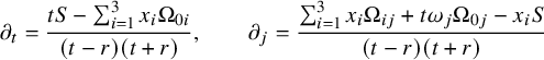 $$ \begin{align*} \partial_t&=\frac{tS-\sum_{i=1}^3x_i\Omega_{0i}}{(t-r)(t+r)},\qquad \partial_j=\frac{\sum_{i=1}^3 x_i\Omega_{ij}+t\omega_j\Omega_{0j}-x_iS}{(t-r)(t+r)} \end{align*} $$
to replace each translation in $Z^I$
with a finite sum of
$Z^I$
with a finite sum of $S,\Omega _{ij},\Omega _{0i}$
multiplied by an explicit function of
$S,\Omega _{ij},\Omega _{0i}$
multiplied by an explicit function of $(t,x)$
. By Leibniz’s rule, one can write
$(t,x)$
. By Leibniz’s rule, one can write
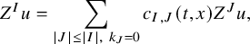 $$ \begin{align}\begin{aligned} Z^Iu&=\sum_{|J|\leq |I|,\ k_J=0}c_{I,J}(t,x)Z^Ju ,\end{aligned}\end{align} $$
where $k_J$
denotes the number of translations in
$k_J$
denotes the number of translations in $Z^J$
and
$Z^J$
and $c_{I,J}(t,x)$
can be computed explicitly from the coefficients in [Reference Lindblad45, (3.1)]. Combining this expression and (1.23), we thus obtain a more accurate asymptotic formula for
$c_{I,J}(t,x)$
can be computed explicitly from the coefficients in [Reference Lindblad45, (3.1)]. Combining this expression and (1.23), we thus obtain a more accurate asymptotic formula for $Z^Iu$
when
$Z^Iu$
when $Z^I$
contains translations.
$Z^I$
contains translations.
We also remark that $c_{I,J}=O((t-r)^{-k_I})$
whenever
$c_{I,J}=O((t-r)^{-k_I})$
whenever $r<t-1$
and
$r<t-1$
and $t\gg 1$
. In other words, by setting
$t\gg 1$
. In other words, by setting $\widetilde { c }_{I,J}=(t-r)^{k_I}c_{I,J}=O(1)$
, we obtain
$\widetilde { c }_{I,J}=(t-r)^{k_I}c_{I,J}=O(1)$
, we obtain
 $$ \begin{align}\begin{aligned} (t-r)^{k_I}Z^Iu(t,x)&=-\frac{\varepsilon}{4\pi}\sum_{|J|\leq |I|,\ k_J=0}\widetilde{ c }_{I,J}(t,x)\int_{\mathbb{S}^2}A_J(x\cdot \theta-t,\theta)\ dS_\theta+O_{|I|}(\langle t-|x| \rangle^{-2}t^{C_{|I|}\varepsilon}) \end{aligned}\end{align} $$
for all $t\geq e^{\delta /\varepsilon }$
and
$t\geq e^{\delta /\varepsilon }$
and $|x|< t-1$
. When
$|x|< t-1$
. When $Z^I$
contains translations, the estimate (1.26) is a more accurate asymptotic formula for
$Z^I$
contains translations, the estimate (1.26) is a more accurate asymptotic formula for $Z^Iu$
. For simplicity, we do not present the formulas for
$Z^Iu$
. For simplicity, we do not present the formulas for $\widetilde { c }_{I,J}$
here, but we emphasize that they can be computed explicitly.
$\widetilde { c }_{I,J}$
here, but we emphasize that they can be computed explicitly.
Remark 1.5. We now have a full description of the asymptotic behaviors of the global solution u to (1.1) and (1.2). First, Theorem 1 provides a good approximation for $Z^Iu$
for
$Z^Iu$
for $t\gg _{\delta ,\varepsilon }1$
and
$t\gg _{\delta ,\varepsilon }1$
and $|x|<t-t^{1/2+}$
. Moreover, we obtain from [Reference Yu75] an approximation for u whenever
$|x|<t-t^{1/2+}$
. Moreover, we obtain from [Reference Yu75] an approximation for u whenever $t\gg _{\delta ,\varepsilon }1$
and
$t\gg _{\delta ,\varepsilon }1$
and $|x|>t-t^{1-}$
. For each multiindex I, we have
$|x|>t-t^{1-}$
. For each multiindex I, we have
 $$ \begin{align*} Z^Iu(t,x)=Z^I\widetilde{ u }(t,x)+O_{\gamma,|I|}(\varepsilon t^{-2+C_{I}\varepsilon}\langle r-t \rangle) \end{align*} $$
whenever $t\geq 2e^{\delta /\varepsilon }$
and
$t\geq 2e^{\delta /\varepsilon }$
and $|r-t|\lesssim t^\gamma $
for each fixed
$|r-t|\lesssim t^\gamma $
for each fixed $\gamma \in (0,1)$
. Also see (3.14) in Section 3.4. Here,
$\gamma \in (0,1)$
. Also see (3.14) in Section 3.4. Here, $\widetilde { u }$
is defined in both Section 1.2.3 and Section 3.4. We also recall that
$\widetilde { u }$
is defined in both Section 1.2.3 and Section 3.4. We also recall that $u\equiv 0$
whenever
$u\equiv 0$
whenever $r-t\geq R$
, where
$r-t\geq R$
, where $R>0$
is a constant such that the initial data (1.2) vanishes for
$R>0$
is a constant such that the initial data (1.2) vanishes for $|x|\geq R$
. In other words, for all
$|x|\geq R$
. In other words, for all $(t,x)$
with
$(t,x)$
with $t\gg _{\delta ,\varepsilon }1$
, we have at least one way to approximate
$t\gg _{\delta ,\varepsilon }1$
, we have at least one way to approximate $Z^Iu(t,x)$
.
$Z^Iu(t,x)$
.
Remark 1.6. The proof of (1.23) is robust and does not only work for (1.1). Let $\phi =\phi (t,x)$
be a
$\phi =\phi (t,x)$
be a $C^2$
function defined for all
$C^2$
function defined for all $t>0$
and
$t>0$
and $|x|<t$
. If
$|x|<t$
. If $\Box \phi $
satisfies a good pointwise bound, and if we have a good way to approximate
$\Box \phi $
satisfies a good pointwise bound, and if we have a good way to approximate $(-\partial _t+\partial _r)(r\phi )$
near the light cone
$(-\partial _t+\partial _r)(r\phi )$
near the light cone $r=t$
for all
$r=t$
for all $t\gg 1$
, then we can prove an asymptotic formula for
$t\gg 1$
, then we can prove an asymptotic formula for $\phi $
similar to (1.23). In fact, approximately, one can apply Proposition 4.1 to show that
$\phi $
similar to (1.23). In fact, approximately, one can apply Proposition 4.1 to show that
 $$ \begin{align}\begin{aligned} \phi(t,x)&\approx-\frac{1}{4\pi}\int_{\mathbb{S}^2}\mathcal{ A }_0(x\cdot\theta-t,\theta)\ dS_\theta,\qquad \forall |x|<t,\ t\gg1. \end{aligned}\end{align} $$
Here, $\mathcal { A }_0$
is the radiation field for
$\mathcal { A }_0$
is the radiation field for $\phi _t-\phi _r$
in the sense that
$\phi _t-\phi _r$
in the sense that
 $$ \begin{align*} \phi_t-\phi_r\approx r^{-1}\mathcal{ A }_0(r-t,\omega),\qquad \text{whenever }|r-t|\ll t. \end{align*} $$
For a nonrigorous derivation of this approximate identity, we refer to the discussion above (1.35) in Section 1.4. The form of the error term in (1.27) depends on the pointwise bounds for $\phi $
and
$\phi $
and $\Box \phi $
, and we will not discuss it in detail here for simplicity.
$\Box \phi $
, and we will not discuss it in detail here for simplicity.
Remark 1.7. We now discuss how (1.27) is related to [Reference Lindblad and Schlue49, Theorem 1.5]. Recall that the authors of [Reference Lindblad and Schlue49] constructed a global solution $\phi $
to
$\phi $
to $\Box \phi =0$
with a prescribed radiation field and then described the interior and exterior asymptotics of
$\Box \phi =0$
with a prescribed radiation field and then described the interior and exterior asymptotics of $\phi $
. In particular, they mentioned that
$\phi $
. In particular, they mentioned that $\phi $
has the interior homogeneous asymptotics [Reference Lindblad and Schlue49, (1.11)]:
$\phi $
has the interior homogeneous asymptotics [Reference Lindblad and Schlue49, (1.11)]:
 $$ \begin{align}\begin{aligned} \phi(t,x)\approx\frac{1}{4\pi}\int_{\mathbb{S}^2}\frac{N(\theta)}{t-x\cdot \theta}\ dS_\theta,\qquad \text{for } |x|/t<1\text{ fixed},\ t\to\infty. \end{aligned}\end{align} $$
Interestingly, given the radiation field of $\phi _t$
in [Reference Lindblad and Schlue49, Theorem 1.5], one can nonrigorously derive (1.28) to the leading order by (1.27). In [Reference Lindblad and Schlue49, Remark 1.3], it was mentioned that
$\phi _t$
in [Reference Lindblad and Schlue49, Theorem 1.5], one can nonrigorously derive (1.28) to the leading order by (1.27). In [Reference Lindblad and Schlue49, Remark 1.3], it was mentioned that $\phi _t$
has the radiation field
$\phi _t$
has the radiation field
 $$ \begin{align*} \phi_t\approx r^{-1}\mathcal{ G }_0(r-t,\omega),\qquad \text{with }\mathcal{ G }_0=N_{01}(\omega)q\langle q \rangle^{-2}-\partial_q\mathcal{ F }_{01}(q,\omega). \end{align*} $$
Both $N_{01}$
and
$N_{01}$
and $\mathcal { F }_{01}$
are from the statement of [Reference Lindblad and Schlue49, Theorem 1.5]. When
$\mathcal { F }_{01}$
are from the statement of [Reference Lindblad and Schlue49, Theorem 1.5]. When $q<-1$
, we have
$q<-1$
, we have $\partial _q\mathcal { F }_{01}=O(\langle q \rangle ^{-2})$
, which is a lower order term compared to
$\partial _q\mathcal { F }_{01}=O(\langle q \rangle ^{-2})$
, which is a lower order term compared to $N_{01}(\omega )q\langle q \rangle ^{-2}$
. Since
$N_{01}(\omega )q\langle q \rangle ^{-2}$
. Since $\phi _t+\phi _r$
is a tangential derivative, we expect
$\phi _t+\phi _r$
is a tangential derivative, we expect $\phi _r\approx -\phi _t$
, so
$\phi _r\approx -\phi _t$
, so $\phi _t-\phi _r\approx 2\mathcal { G }_0\approx 2N_{01}q^{-1}$
whenever
$\phi _t-\phi _r\approx 2\mathcal { G }_0\approx 2N_{01}q^{-1}$
whenever $q<0$
and
$q<0$
and $|q|\gg 1$
. Plug this into (1.27), and we obtain
$|q|\gg 1$
. Plug this into (1.27), and we obtain
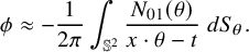 $$ \begin{align*} \phi\approx -\frac{1}{2\pi}\int_{\mathbb{S}^2}\frac{N_{01}(\theta)}{x\cdot\theta-t}\ dS_\theta. \end{align*} $$
Remark 1.8. The formula (1.23) can also be extended to a scalar quasilinear wave equation satisfying the null condition:
 $$ \begin{align}\begin{aligned} g^{\alpha\beta}(u,\partial u)\partial_\alpha\partial_\beta u=f(u,\partial u). \end{aligned}\end{align} $$
The Cauchy problem (1.29) and (1.2) admits a global solution u. One can also show that the following limit exists and is a continuous function:
 $$ \begin{align*} B(q,\omega):=\lim_{r\to\infty}(-\partial_t+\partial_r)(ru)(r-q,r\omega). \end{align*} $$
By Proposition 4.1, we can show not only (1.27) but also a more precise estimate
 $$ \begin{align}\begin{aligned} u(t,x)&=\frac{1}{4\pi}\int_{\mathbb{S}^2}B(x\cdot\theta-t,\theta)\ dS_\theta+O(t^{-1}\langle t-|x| \rangle^{-3}),\qquad \forall t>1,|x|<t. \end{aligned}\end{align} $$
This estimate is weaker than the results in [Reference Dong, Ma, Ma and Yuan18, Reference Luk and Oh54, Reference Luk and Oh53], but it provides a potentially different way to prove the results in those papers. To recover, for example, [Reference Dong, Ma, Ma and Yuan18, (1.12)], one needs an asymptotic formula for B as follows:
 $$ \begin{align}\begin{aligned} B(q,\omega)=c_0q^{-2}+O(|q|^{-3}),\qquad \forall q<-1, \text{for some constant }c_0. \end{aligned}\end{align} $$
If it is true, then we have
 $$ \begin{align*} u(t,x)&=\frac{1}{4\pi}\int_{\mathbb{S}^2}c_0(x\cdot\theta-t)^{-2}+O(|x\cdot\theta-t|^{-3})\ dS_\theta+O(t^{-1}\langle t-|x| \rangle^{-3})\\ &= c_0(t^2-|x|^2)^{-1}+O( t^{-1}\langle t-|x| \rangle^{-2}) \end{align*} $$
for all $t>1$
and
$t>1$
and $|x|<t-1$
. If one can furthermore prove that
$|x|<t-1$
. If one can furthermore prove that $c_0=0$
, then we obtain the better pointwise decay rate
$c_0=0$
, then we obtain the better pointwise decay rate $u=O(t^{-1}\langle |x|-t \rangle ^{-2})$
in [Reference Dong, Ma, Ma and Yuan18, Reference Luk and Oh54, Reference Luk and Oh53]. It is, however, unclear to the author whether one can show the asymptotics (1.31) and
$u=O(t^{-1}\langle |x|-t \rangle ^{-2})$
in [Reference Dong, Ma, Ma and Yuan18, Reference Luk and Oh54, Reference Luk and Oh53]. It is, however, unclear to the author whether one can show the asymptotics (1.31) and $c_0=0$
, so we do not claim in this paper that we have given different proofs of those results.
$c_0=0$
, so we do not claim in this paper that we have given different proofs of those results.
By (1.23), we can show several interesting properties of global solutions to (1.1) when the null condition is violated. All but one of them fail if the null condition is satisfied.
Recall that the null condition was defined for a general system (1.5) in Section 1.1. By (1.10), the equation (1.1) satisfies the null condition if and only if $G(\omega )\equiv 0$
on
$G(\omega )\equiv 0$
on $\mathbb {S}^2$
, with
$\mathbb {S}^2$
, with $G(\omega )$
defined by (1.11). Since
$G(\omega )$
defined by (1.11). Since $g^{00}\equiv -1$
, we claim that
$g^{00}\equiv -1$
, we claim that $G(\omega )\equiv 0$
on
$G(\omega )\equiv 0$
on $\mathbb {S}^2$
if and only if
$\mathbb {S}^2$
if and only if $g^{\alpha \beta }_0=0$
for all
$g^{\alpha \beta }_0=0$
for all $\alpha ,\beta =0,1,2,3$
. In fact, if
$\alpha ,\beta =0,1,2,3$
. In fact, if $G(\omega )\equiv 0$
on
$G(\omega )\equiv 0$
on $\mathbb {S}^2$
, we have a decomposition
$\mathbb {S}^2$
, we have a decomposition
 $$ \begin{align*} (g^{\alpha\beta}_0)=g^{00}_0\text{diag}(1,-1,-1,-1)+(\text{an asymmetric matrix}). \end{align*} $$
Since $(g^{\alpha \beta })$
is symmetric, so is
$(g^{\alpha \beta })$
is symmetric, so is $(g^{\alpha \beta }_0)$
. Thus, the asymmetric part in this decomposition vanishes. And since
$(g^{\alpha \beta }_0)$
. Thus, the asymmetric part in this decomposition vanishes. And since $g^{00}\equiv -1$
, we have
$g^{00}\equiv -1$
, we have $g^{00}_0=0$
and thus
$g^{00}_0=0$
and thus $g^{\alpha \beta }_0=0$
.
$g^{\alpha \beta }_0=0$
.
We first state a theorem related to the scattering data.
Theorem 2. Suppose that the equation (1.1) violates the null condition. Fix $(u_0,u_1)\in C_c^\infty (\mathbb {R}^3)$
. Let u be the global solution to (1.1) with initial data (1.2) for
$(u_0,u_1)\in C_c^\infty (\mathbb {R}^3)$
. Let u be the global solution to (1.1) with initial data (1.2) for $\varepsilon \ll 1$
. Fix a small
$\varepsilon \ll 1$
. Fix a small $\delta \in (0,1)$
and let
$\delta \in (0,1)$
and let $\widehat { A }$
be the corresponding scattering data.
$\widehat { A }$
be the corresponding scattering data.
Moreover, suppose that one of the following assumptions holds:
-
a) We have $\min _{(q,\omega )\in \mathbb {R}\times \mathbb {S}^2}\widehat { A }(q,\omega )\geq 0$
or
$\max _{(q,\omega )\in \mathbb {R}\times \mathbb {S}^2}\widehat { A }(q,\omega )\leq 0$
;
$\min _{(q,\omega )\in \mathbb {R}\times \mathbb {S}^2}\widehat { A }(q,\omega )\geq 0$
or
$\max _{(q,\omega )\in \mathbb {R}\times \mathbb {S}^2}\widehat { A }(q,\omega )\leq 0$
; -
b) We have
$\min _{ \omega \in \mathbb {S}^2}G(\omega )\geq 0$
and
$\min \{\widehat { A },0\}\in L^1_{q,\omega }(\mathbb {R}\times \mathbb {S}^2)$
, or we have
$\max _{ \omega \in \mathbb {S}^2}G(\omega )\leq 0$
and
$\max \{\widehat { A },0\}\in L^1_{q,\omega }(\mathbb {R}\times \mathbb {S}^2)$
; -
c) Let
$C_0>0$
be a constant uniform in all
$\varepsilon \ll 1$
such that Such a
$$ \begin{align*} C_0\geq \sup_{(q,\omega)\in\mathbb{R}\times\mathbb{S}^2}|\frac{1}{2} G(\omega)\widehat{ A }(q,\omega)|. \end{align*} $$
$C_0$
always exists because of (1.20). Suppose that there exists a constant
$B_0>C_0$
that is also uniform in all
$\varepsilon \ll 1$
, such that
$$ \begin{align*} \lim_{q\to-\infty}\langle q \rangle^{1+B_0\varepsilon}\sup_{\omega\in\mathbb{S}^2}|\widehat{ A }(q,\omega)|=0. \end{align*} $$


Then, as long as $\varepsilon \ll 1$
(depending on the constant
$\varepsilon \ll 1$
(depending on the constant $B_0$
in part c)), we have
$B_0$
in part c)), we have $\widehat { A }\equiv 0$
and thus
$\widehat { A }\equiv 0$
and thus $u\equiv 0$
.
$u\equiv 0$
.
Remark 2.1. The assumption a) implies $\widehat { A }\equiv 0$
and
$\widehat { A }\equiv 0$
and $u\equiv 0$
no matter whether (1.1) satisfies the null condition. We refer to Section 6.2.1 and Footnote 15. However, for b) and c), it is necessary to assume that the null condition is violated. Suppose that (1.1) satisfies the null condition, and let u be a global solution to (1.1) and (1.2). One can check that
$u\equiv 0$
no matter whether (1.1) satisfies the null condition. We refer to Section 6.2.1 and Footnote 15. However, for b) and c), it is necessary to assume that the null condition is violated. Suppose that (1.1) satisfies the null condition, and let u be a global solution to (1.1) and (1.2). One can check that
 $$ \begin{align}\begin{aligned} \sum_{|I|\leq N}|Z^I u(t,x)|\lesssim\varepsilon t^{-1}\langle |x|-t \rangle^{-1},\qquad \text{as long as }\varepsilon\ll_N1. \end{aligned}\end{align} $$
The case $N=0$
has been proved in Christodoulou [Reference Christodoulou11]. For
$N=0$
has been proved in Christodoulou [Reference Christodoulou11]. For $N>0$
, one can apply the estimates in [Reference Hörmander26, Section 6.6] and [Reference Alinhac3, Proposition 3.1]. Following the proofs in [Reference Yu75, Section 5.4], from these pointwise bounds we obtain
$N>0$
, one can apply the estimates in [Reference Hörmander26, Section 6.6] and [Reference Alinhac3, Proposition 3.1]. Following the proofs in [Reference Yu75, Section 5.4], from these pointwise bounds we obtain $|\widehat { A }(q,\omega )|\lesssim \langle q \rangle ^{-2}$
. In other words, the assumptions b) and c) hold in general.
$|\widehat { A }(q,\omega )|\lesssim \langle q \rangle ^{-2}$
. In other words, the assumptions b) and c) hold in general.
Remark 2.2. Let us compare the assumption c) with the pointwise bound (1.20) for $\widehat { A }$
. By (1.20), we have
$\widehat { A }$
. By (1.20), we have $|\widehat { A }(q,\omega )|\lesssim \langle q \rangle ^{-1+C\varepsilon }$
for all
$|\widehat { A }(q,\omega )|\lesssim \langle q \rangle ^{-1+C\varepsilon }$
for all $(q,\omega )\in \mathbb {R}\times \mathbb {S}^2$
. Part c) of Theorem 2 indicates that if the null condition is violated and if
$(q,\omega )\in \mathbb {R}\times \mathbb {S}^2$
. Part c) of Theorem 2 indicates that if the null condition is violated and if $|\widehat { A }(q,\omega )|\lesssim \langle q \rangle ^{-1-B_0\varepsilon }$
everywhere for a large constant
$|\widehat { A }(q,\omega )|\lesssim \langle q \rangle ^{-1-B_0\varepsilon }$
everywhere for a large constant $B_0>1$
, then
$B_0>1$
, then $u\equiv 0$
as long as
$u\equiv 0$
as long as $\varepsilon \ll 1$
. In other words, if the null condition is violated, the scattering data cannot decay arbitrarily fast in all directions as
$\varepsilon \ll 1$
. In other words, if the null condition is violated, the scattering data cannot decay arbitrarily fast in all directions as $q\to -\infty $
. Besides, the exponent
$q\to -\infty $
. Besides, the exponent $-1+C\varepsilon $
in
$-1+C\varepsilon $
in $|\widehat { A }(q,\omega )|\lesssim \langle q \rangle ^{-1+C\varepsilon }$
is almost sharp.
$|\widehat { A }(q,\omega )|\lesssim \langle q \rangle ^{-1+C\varepsilon }$
is almost sharp.
We also compare the assumption c) with the assumption (1.19) in the modified wave operator problem. There we assume that $|\widehat { A }|\lesssim \langle q \rangle ^{-2-}$
, so the global solutions constructed in [Reference Yu74, Reference Yu73] cannot have compactly supported initial data if the null condition is violated. It is unclear whether one can further relax the assumption (1.19) in the modified wave operator problem. For example, can we assume
$|\widehat { A }|\lesssim \langle q \rangle ^{-2-}$
, so the global solutions constructed in [Reference Yu74, Reference Yu73] cannot have compactly supported initial data if the null condition is violated. It is unclear whether one can further relax the assumption (1.19) in the modified wave operator problem. For example, can we assume $\gamma _->1$
instead of
$\gamma _->1$
instead of $\gamma _->2$
?
$\gamma _->2$
?
The scattering $\widehat { A }$
satisfies an extra decaying property. By Proposition 6.1, we have
$\widehat { A }$
satisfies an extra decaying property. By Proposition 6.1, we have
 $$ \begin{align*} |\int_{\mathbb{S}^2}\widehat{ U }(\varepsilon\ln t-\delta,-2t,\omega )dS_\omega|\lesssim\varepsilon^{-1}t^{-1/3+C\varepsilon},\qquad \forall t\geq 2e^{\delta/\varepsilon}, \end{align*} $$
where (recall that $R>0$
is chosen so that the data (1.2) vanishes for
$R>0$
is chosen so that the data (1.2) vanishes for $|x|\geq R$
)
$|x|\geq R$
)
 $$ \begin{align*} \widehat{ U }(s,q,\omega)=-\int_{q}^R\widehat{ A }(p,\omega)\exp(\frac{1}{2}G(\omega)\widehat{ A }(p,\omega) s)\ dp. \end{align*} $$
In contrast, from $\widehat { A }=O(\langle q \rangle ^{-1+C\varepsilon })$
, we only have
$\widehat { A }=O(\langle q \rangle ^{-1+C\varepsilon })$
, we only have $\widehat { U }(s,q,\omega )=O(\varepsilon ^{-1}\langle q \rangle ^{C\varepsilon }e^{Cs})$
and
$\widehat { U }(s,q,\omega )=O(\varepsilon ^{-1}\langle q \rangle ^{C\varepsilon }e^{Cs})$
and $\widehat { U }(\varepsilon \ln t-\delta ,-2t,\omega )=O(\varepsilon ^{-1}t^{C\varepsilon })$
. Because of part c), we cannot improve this bound for
$\widehat { U }(\varepsilon \ln t-\delta ,-2t,\omega )=O(\varepsilon ^{-1}t^{C\varepsilon })$
. Because of part c), we cannot improve this bound for $\widehat { U }$
if we only rely on the pointwise bounds for
$\widehat { U }$
if we only rely on the pointwise bounds for $\widehat { A }$
. Thus, to relax the assumption (1.19) in the modified wave operator problem, we may also need to take such a decaying property into account.
$\widehat { A }$
. Thus, to relax the assumption (1.19) in the modified wave operator problem, we may also need to take such a decaying property into account.
We now state a corollary of Theorem 2. Here, we focus on the pointwise decay for the solutions and their first derivatives.
Theorem 3. Suppose that (1.1) violates the null condition. Fix $(u_0,u_1)\in C_c^\infty (\mathbb {R}^3)$
. Let u be the global solution to (1.1) with initial data (1.2) for
$(u_0,u_1)\in C_c^\infty (\mathbb {R}^3)$
. Let u be the global solution to (1.1) with initial data (1.2) for $\varepsilon \ll 1$
. Suppose that there exist constants
$\varepsilon \ll 1$
. Suppose that there exist constants $B_0,B_1>0$
depending on
$B_0,B_1>0$
depending on $u_0,u_1$
(but not on
$u_0,u_1$
(but not on $\varepsilon $
), such that one of the following assumptions holds:
$\varepsilon $
), such that one of the following assumptions holds:
-
i) Fix
$0<\nu _0<1$
. For all
$t\geq 1$
and
$\omega \in \mathbb {S}^2$
, we have
$$ \begin{align*} |(u_t-u_r)(t,(t-t^{\nu_0})\omega)|\lesssim \varepsilon t^{-1-\nu_0-\nu_0B_0\varepsilon}; \end{align*} $$
-
ii) Fix
$0<\nu _0<1$
. For all
$t\geq 2$
and
$x\in \mathbb {R}^3$
with
$|x|\in [t-2t^{\nu _0},t-t^{\nu _0}/2]$
, we have
$$ \begin{align*} |u(t,x) |\lesssim\varepsilon t^{-1-(\nu_0 B_0+B_1)\varepsilon}; \end{align*} $$
-
iii) Suppose that u is a spherically symmetric solution with respect to x and that
$$ \begin{align*} |u(t,0)|\lesssim\varepsilon t^{-1-B_0\varepsilon} \qquad \forall t\geq 1. \end{align*} $$


Then, as long as $\varepsilon \ll 1$
, which may depend on the constants in each of the assumptions, we have
$\varepsilon \ll 1$
, which may depend on the constants in each of the assumptions, we have $u \equiv 0$
.
$u \equiv 0$
.
Remark 3.1. Note that the assumptions i) and ii) are related to the pointwise decays of u and $\partial u$
for
$\partial u$
for $|r-t|\lesssim t^{\nu _0}$
. Recall from [Reference Lindblad45] that
$|r-t|\lesssim t^{\nu _0}$
. Recall from [Reference Lindblad45] that $|\partial u|\lesssim \varepsilon t^{-1}\langle r-t \rangle ^{-1+C\varepsilon }$
and
$|\partial u|\lesssim \varepsilon t^{-1}\langle r-t \rangle ^{-1+C\varepsilon }$
and $|u|\lesssim \varepsilon t^{-1+C\varepsilon }$
. Thus, both the exponents
$|u|\lesssim \varepsilon t^{-1+C\varepsilon }$
. Thus, both the exponents $-1+C\varepsilon $
in these estimates are almost sharp if the null condition is violated.
$-1+C\varepsilon $
in these estimates are almost sharp if the null condition is violated.
If the null condition is satisfied, then as shown in (1.32) in Remark 2.1, we have $|\partial u|\lesssim \varepsilon t^{-1}\langle r-t \rangle ^{-2}$
and
$|\partial u|\lesssim \varepsilon t^{-1}\langle r-t \rangle ^{-2}$
and $|u|\lesssim \varepsilon t^{-1}\langle r-t \rangle ^{-1}$
. That is, the assumptions i) and ii) hold in general.
$|u|\lesssim \varepsilon t^{-1}\langle r-t \rangle ^{-1}$
. That is, the assumptions i) and ii) hold in general.
Remark 3.2. We now prove the fact stated in Remark 1.3. Suppose that the null condition is violated. Let u be a nonzero global solution to (1.1) and (1.2) with $\varepsilon \ll 1$
. If we take
$\varepsilon \ll 1$
. If we take $\nu _0=3/4$
(or any number in
$\nu _0=3/4$
(or any number in $(1/2,1)$
) in part ii) of Theorem 3, we obtain a sequence of points
$(1/2,1)$
) in part ii) of Theorem 3, we obtain a sequence of points $\{(t_n,x_n)\}$
with
$\{(t_n,x_n)\}$
with
 $$ \begin{align*} t_n\uparrow\infty,\qquad 0<t_n-|x_n|\sim t^{3/4},\qquad |u(t_n,x_n)|\geq \varepsilon t^{-1-C_{B_0,B_1}\varepsilon}. \end{align*} $$
We also have
 $$ \begin{align*} \langle |x_n|-t_n \rangle^{-2}t_n^{C\varepsilon}\lesssim t_n^{-3/2+C\varepsilon}\ll \varepsilon t_n^{-1-C_{B_0,B_1}\varepsilon},\qquad \forall t\geq e^{\delta/\varepsilon}. \end{align*} $$
In other words, the estimate (1.24) must fail for this sequence of points.
Remark 3.3. Part iii) of Theorem 3 suggests that, if the null condition is violated, and if the solution is spherically symmetric with respect to x, then $u(t,0)$
cannot decay arbitrarily fast as
$u(t,0)$
cannot decay arbitrarily fast as $t\to \infty $
. Unlike the assumptions i) and ii), here we make an assumption on the decay rate of u along the time-axis which is far inside the light cone. In Proposition 6.6 below), we can replace the spherical symmetry condition with an assumption on the decay rate of
$t\to \infty $
. Unlike the assumptions i) and ii), here we make an assumption on the decay rate of u along the time-axis which is far inside the light cone. In Proposition 6.6 below), we can replace the spherical symmetry condition with an assumption on the decay rate of $\partial \Omega _{ij}u$
near the light cone.
$\partial \Omega _{ij}u$
near the light cone.
It is, however, unclear to the author whether the spherical symmetry condition and the assumption on the decay rate of $\partial \Omega _{ij}u$
can be completely removed. For example, assuming
$\partial \Omega _{ij}u$
can be completely removed. For example, assuming
 $$ \begin{align*} |u(t,x)|&\lesssim \varepsilon t^{-1-},\qquad \forall t\geq 1,\ |x|\leq t/2, \end{align*} $$
can we show $u\equiv 0$
for
$u\equiv 0$
for $\varepsilon \ll 1$
?
$\varepsilon \ll 1$
?
1.4 Structure of this paper
We now explain how this paper is organized. We also invite our readers to check the beginning of each of Sections 3–6 for an overview of that specific section.
In Section 2, we introduce the notation and several preliminary lemmas. We emphasize that a special convention involving $\varepsilon $
is made in Section 2.2.
$\varepsilon $
is made in Section 2.2.
In Section 3, we present an overview of the asymptotic completeness result for (1.1). We follow the discussion in Section 1.2.3 and provide more details. We will also prove several results that did not appear in [Reference Yu75]. For example, in Proposition 3.3, we provide an asymptotic formula for higher derivatives of $\widehat { u }$
which was constructed from our scattering data in [Reference Yu75, Section 7]. In Section 3.6, we provide a new gauge independence result which is stated in a much cleaner way than [Reference Yu75, Proposition 6.1].
$\widehat { u }$
which was constructed from our scattering data in [Reference Yu75, Section 7]. In Section 3.6, we provide a new gauge independence result which is stated in a much cleaner way than [Reference Yu75, Proposition 6.1].
In Section 4, we study a general inhomogeneous wave equation $\Box \phi =F$
inside the light cone
$\Box \phi =F$
inside the light cone $|x|=t$
. Assuming that
$|x|=t$
. Assuming that
 $$ \begin{align}\begin{aligned} |F(t,x)|\lesssim \langle t \rangle^{-\gamma_1}\langle r-t \rangle^{-\gamma_2},\qquad \text{in }\mathcal{O}=\{t>0,|x|<t\},\ \text{with }\gamma_1,\gamma_2>0, \end{aligned}\end{align} $$
we derive an asymptotic formula for $\phi $
: whenever
$\phi $
: whenever $(t,x)\in \mathcal {O}$
and whenever
$(t,x)\in \mathcal {O}$
and whenever $T>2t$
, we have
$T>2t$
, we have
 $$ \begin{align}\begin{aligned} \phi(t,x)&=\frac{1}{4\pi}\int_{\mathbb{S}^2}\Phi(T,x-(T-t)\theta)\ dS_\theta+\text{(a remainder term)},\quad \text{with }\Phi:=(-\partial_t+\partial_r)(|x|\phi). \end{aligned}\end{align} $$
See Proposition 4.1. In its proof, we view $\phi $
as a solution to the backward Cauchy problem
$\phi $
as a solution to the backward Cauchy problem $\Box \phi =F$
with initial data assigned at
$\Box \phi =F$
with initial data assigned at $t=T$
, so we can express
$t=T$
, so we can express $\phi (t,x)$
explicitly as a sum of an integral of F and an integral of
$\phi (t,x)$
explicitly as a sum of an integral of F and an integral of $(\phi ,\phi _t)|_{t=T}$
. We use (1.33) to control the integral of F, so
$(\phi ,\phi _t)|_{t=T}$
. We use (1.33) to control the integral of F, so $\phi $
is approximated well by the solution to
$\phi $
is approximated well by the solution to $\Box w=0$
with data
$\Box w=0$
with data $(\phi ,\phi _t)|_{t=T}$
at
$(\phi ,\phi _t)|_{t=T}$
at $t=T$
. Direct computations yield (1.34).
$t=T$
. Direct computations yield (1.34).
The formula (1.34) is useful in this paper because one can relate the integral of $\Phi $
with the asymptotics of
$\Phi $
with the asymptotics of $\phi $
at null infinity. In fact, we will prove in Lemma 5.1 that
$\phi $
at null infinity. In fact, we will prove in Lemma 5.1 that
 $$ \begin{align*} \lim_{T\to\infty}(|x-(T-t)\theta|-T,\frac{x-(T-t)\theta}{|x-(T-t)\theta|})=(-t-x\cdot \theta,-\theta),\qquad \forall t>|x|>0,\ \theta\in\mathbb{S}^2. \end{align*} $$
In other words, the curve $T\mapsto (T,x-(T-t)\theta )$
converges to the straight line
$T\mapsto (T,x-(T-t)\theta )$
converges to the straight line $T\mapsto (T,(x+t\cdot \theta -T)\theta )$
as
$T\mapsto (T,(x+t\cdot \theta -T)\theta )$
as $T\to \infty $
. If the radiation field of
$T\to \infty $
. If the radiation field of $\phi _t-\phi _r$
 $$ \begin{align*} \mathcal{ A }_0(q,\omega)=\lim_{r\to\infty}r(\phi_t-\phi_r)(r-q,r\omega) \end{align*} $$
exists for all $(q,\omega )\in \mathbb {R}\times \mathbb {S}^2$
, then we expect
$(q,\omega )\in \mathbb {R}\times \mathbb {S}^2$
, then we expect
 $$ \begin{align*} \lim_{T\to\infty}\int_{\mathbb{S}^2}\Phi(T,x-(T-t)\theta)\ dS_\theta=-\frac{1}{4\pi}\int_{\mathbb{S}^2}\mathcal{ A }_0(-t-x\cdot\theta,-\theta)\ dS_\theta. \end{align*} $$
If one can also control the remainder term (1.34) when $T\to \infty $
, then we have
$T\to \infty $
, then we have
 $$ \begin{align}\begin{aligned} \phi(t,x)=-\frac{1}{4\pi}\int_{\mathbb{S}^2}\mathcal{ A }_0(x\cdot\theta-t,\theta)\ dS_\theta+\text{(a remainder term)},\qquad \forall (t,x)\in\mathcal{ O }. \end{aligned}\end{align} $$
Unfortunately, if u solves (1.1), $u_t-u_r$
does not necessarily admit a radiation field in the usual sense. In other words, we cannot apply (1.35) directly to finish the proof of Theorem 1. We thus require a more delicate analysis of the asymptotic behaviors of u near the light cone.
$u_t-u_r$
does not necessarily admit a radiation field in the usual sense. In other words, we cannot apply (1.35) directly to finish the proof of Theorem 1. We thus require a more delicate analysis of the asymptotic behaviors of u near the light cone.
In Section 5, we prove Theorem 1 by combining Proposition 4.1 with the results in Section 3. For each multiindex I, we first prove a pointwise estimate for $\Box Z^Iu$
. Then, by Proposition 4.1, we notice that it remains to estimate the integral
$\Box Z^Iu$
. Then, by Proposition 4.1, we notice that it remains to estimate the integral
 $$ \begin{align*} \int_{\mathbb{S}^2}[(-\partial_t+\frac{y}{|y|}\cdot \partial_y)(|y|Z^Iu)](T,y(t,x,T,\theta))\ dS_\theta. \end{align*} $$
Here, $y(t,x,T,\theta )=x-(T-t)\theta $
. In our proof, we set
$y(t,x,T,\theta )=x-(T-t)\theta $
. In our proof, we set $T=t^3$
(or a sufficiently large power of t) and take
$T=t^3$
(or a sufficiently large power of t) and take $t\gg _{\delta ,\varepsilon }1$
and
$t\gg _{\delta ,\varepsilon }1$
and $|x|<t$
. Under this setting, we have
$|x|<t$
. Under this setting, we have $||y|-T|\lesssim T^{1/3}$
, so one can apply Proposition 3.3 to approximate the integrand.
$||y|-T|\lesssim T^{1/3}$
, so one can apply Proposition 3.3 to approximate the integrand.
In Section 6, we prove Theorems 2 and 3. We first notice that Theorem 3 follows from part c) of Theorem 2. That is, we need to show $\widehat { A }=O(\langle q \rangle ^{-1-B_0\varepsilon })$
under one of the assumptions i)–iii). To achieve this goal, we apply either (3.14) or (1.23) to transfer the pointwise bounds for u or
$\widehat { A }=O(\langle q \rangle ^{-1-B_0\varepsilon })$
under one of the assumptions i)–iii). To achieve this goal, we apply either (3.14) or (1.23) to transfer the pointwise bounds for u or $\partial u$
to the bounds for
$\partial u$
to the bounds for $\widehat { A }$
. For example, in the case when u is spherically symmetric in x, the scattering data
$\widehat { A }$
. For example, in the case when u is spherically symmetric in x, the scattering data $\widehat { A }$
is independent of
$\widehat { A }$
is independent of $\omega $
(i.e.,
$\omega $
(i.e., $\widehat { A }=\widehat { A }(q)$
). By (1.23) and the bound
$\widehat { A }=\widehat { A }(q)$
). By (1.23) and the bound $|u(t,0)|\lesssim \varepsilon t^{-1-B_0\varepsilon }$
, we obtain immediately that
$|u(t,0)|\lesssim \varepsilon t^{-1-B_0\varepsilon }$
, we obtain immediately that $|\widehat { A }(-t)|\lesssim t^{-1-B_0\varepsilon }$
. This is exactly what we want, so we conclude the proof of part iii). We also refer our readers to Proposition 6.6, which is slightly stronger than Theorem 3.
$|\widehat { A }(-t)|\lesssim t^{-1-B_0\varepsilon }$
. This is exactly what we want, so we conclude the proof of part iii). We also refer our readers to Proposition 6.6, which is slightly stronger than Theorem 3.
We now explain how to prove Theorem 2. Let us focus on parts b) and c), since the proof of part a) is similar and simpler. The proof relies on the explicit formula (1.16) of solutions to the geometric reduced system (1.14). Recall that in Section 1.2.3, we defined $\widehat { U }$
by
$\widehat { U }$
by
 $$ \begin{align*} \widehat{ U }_q(s,q,\omega)&=\widehat{ A }(q,\omega)\exp(\frac{1}{2}G(\omega)\widehat{ A }(q,\omega)s),\qquad \lim_{q\to\infty}\widehat{ U }(s,q,\omega)=0. \end{align*} $$
We observe that $|\widehat { A }|e^{-Cs}\lesssim |\widehat { U }_q|\lesssim |\widehat { A }|e^{Cs}$
and that
$|\widehat { A }|e^{-Cs}\lesssim |\widehat { U }_q|\lesssim |\widehat { A }|e^{Cs}$
and that $\lim _{s\to \infty }\widehat { U }_q\cdot 1_{G(\omega )\widehat { A }<0}=0$
. Besides, we can show that a certain integral of
$\lim _{s\to \infty }\widehat { U }_q\cdot 1_{G(\omega )\widehat { A }<0}=0$
. Besides, we can show that a certain integral of $\widehat { U }_q$
decays to
$\widehat { U }_q$
decays to $0$
as
$0$
as $t\to \infty $
. For example, we have a decaying property in Remark 2.2 or Proposition 6.1. In part c), we also have a pointwise decay for
$t\to \infty $
. For example, we have a decaying property in Remark 2.2 or Proposition 6.1. In part c), we also have a pointwise decay for $\widehat { U }$
in Lemma 6.4. Now we rewrite the integral of
$\widehat { U }$
in Lemma 6.4. Now we rewrite the integral of $\widehat { U }_q$
as the sum of
$\widehat { U }_q$
as the sum of $\mathcal { I }_++\mathcal { I }_-+\mathcal { I }_0$
, where
$\mathcal { I }_++\mathcal { I }_-+\mathcal { I }_0$
, where $\mathcal { I }_\pm $
denotes the integral of
$\mathcal { I }_\pm $
denotes the integral of $\widehat { U }_q\cdot 1_{\pm G(\omega )\widehat { A }>0}$
and
$\widehat { U }_q\cdot 1_{\pm G(\omega )\widehat { A }>0}$
and $\mathcal { I }_0$
denotes the integral of
$\mathcal { I }_0$
denotes the integral of $\widehat { U }_q\cdot 1_{G(\omega )\widehat { A }=0}$
. We send
$\widehat { U }_q\cdot 1_{G(\omega )\widehat { A }=0}$
. We send $t\to \infty $
and study the asymptotics of these three integrals. Under the assumptions of Theorem 2, we can show that
$t\to \infty $
and study the asymptotics of these three integrals. Under the assumptions of Theorem 2, we can show that $\mathcal { I }_0$
can be neglected (because the null condition is violated), that
$\mathcal { I }_0$
can be neglected (because the null condition is violated), that $\mathcal { I }_+\to 0$
(because
$\mathcal { I }_+\to 0$
(because $\mathcal { I }_-\to 0$
by the Lebesgue dominated convergence theorem), and that
$\mathcal { I }_-\to 0$
by the Lebesgue dominated convergence theorem), and that $e^{Cs}\mathcal { I }_-\to 0$
(because of the good decay rate of the integral of
$e^{Cs}\mathcal { I }_-\to 0$
(because of the good decay rate of the integral of $\widehat { U }_q$
). In summary, we can show that
$\widehat { U }_q$
). In summary, we can show that $\widehat { A }\equiv 0$
and thus
$\widehat { A }\equiv 0$
and thus $u\equiv 0$
. We refer to Section 6.2 for more details.
$u\equiv 0$
. We refer to Section 6.2 for more details.
2 Preliminaries
2.1 Notation
We use C to denote universal positive constants. We write $A\lesssim B$
,
$A\lesssim B$
, $B\gtrsim A$
, or
$B\gtrsim A$
, or $A=O(B)$
if
$A=O(B)$
if $|A|\leq CB$
for some
$|A|\leq CB$
for some $C>1$
. The values of all constants in this paper may vary from line to line. We write
$C>1$
. The values of all constants in this paper may vary from line to line. We write $A\sim B$
if
$A\sim B$
if $A\lesssim B$
and
$A\lesssim B$
and $B\lesssim A$
. We use
$B\lesssim A$
. We use $C_{v}$
,
$C_{v}$
, $\gtrsim _v$
, or
$\gtrsim _v$
, or $\lesssim _v$
if we want to emphasize that the constant depends on a parameter v. Moreover, if we make a statement such as ‘
$\lesssim _v$
if we want to emphasize that the constant depends on a parameter v. Moreover, if we make a statement such as ‘ $|A|\leq CB$
for all v in a certain set V’, then it implies that the constant C can be chosen to be uniform for all
$|A|\leq CB$
for all v in a certain set V’, then it implies that the constant C can be chosen to be uniform for all $v\in V$
.
$v\in V$
.
Unless specified otherwise, we always assume that the Latin indices $i,j,k$
take values in
$i,j,k$
take values in $\{1,2,3\}$
and the Greek indices
$\{1,2,3\}$
and the Greek indices $\alpha ,\beta $
take values in
$\alpha ,\beta $
take values in $\{0,1,2,3\}$
. We use subscript to denote partial derivatives unless specified otherwise. For example,
$\{0,1,2,3\}$
. We use subscript to denote partial derivatives unless specified otherwise. For example, $u_{\alpha \beta }=\partial _\alpha \partial _\beta u$
,
$u_{\alpha \beta }=\partial _\alpha \partial _\beta u$
, $q_r=\partial _rq$
,
$q_r=\partial _rq$
, $A_q=\partial _qA$
, etc. For a fixed integer
$A_q=\partial _qA$
, etc. For a fixed integer $k\geq 0$
, we use
$k\geq 0$
, we use $\partial ^k$
to denote either a specific partial derivative of order k, or the collection of partial derivatives of order k.
$\partial ^k$
to denote either a specific partial derivative of order k, or the collection of partial derivatives of order k.
Given a function $f=f(\omega )$
defined on
$f=f(\omega )$
defined on $\mathbb {S}^2$
, in order to define angular derivatives
$\mathbb {S}^2$
, in order to define angular derivatives $\partial _\omega $
, we first extend f to
$\partial _\omega $
, we first extend f to $\mathbb {R}^3\setminus 0$
by setting
$\mathbb {R}^3\setminus 0$
by setting $f(x):=f(x/|x|)$
and then set
$f(x):=f(x/|x|)$
and then set $\partial _{\omega _i}f:=\partial _{x_i}f|_{\mathbb {S}^2}$
. To prevent confusion, we will only use
$\partial _{\omega _i}f:=\partial _{x_i}f|_{\mathbb {S}^2}$
. To prevent confusion, we will only use $\partial _\omega $
to denote angular derivatives under the coordinate system
$\partial _\omega $
to denote angular derivatives under the coordinate system $(s,q,\omega )$
, and we will never use it under the coordinate system
$(s,q,\omega )$
, and we will never use it under the coordinate system $(t,r,\omega )$
. For a fixed integer
$(t,r,\omega )$
. For a fixed integer $k\geq 0$
, we will use
$k\geq 0$
, we will use $\partial _\omega ^k$
to denote either a specific angular derivative of order k, or the collection of all angular derivatives of order k.
$\partial _\omega ^k$
to denote either a specific angular derivative of order k, or the collection of all angular derivatives of order k.
2.2 Dependence on
$\varepsilon $

In this paper, the parameter $\varepsilon $
always denotes the size of initial data in (1.2). We always assume that
$\varepsilon $
always denotes the size of initial data in (1.2). We always assume that $\varepsilon \ll 1$
which means
$\varepsilon \ll 1$
which means $0<\varepsilon <\varepsilon _0$
for some sufficiently small constant
$0<\varepsilon <\varepsilon _0$
for some sufficiently small constant $0<\varepsilon _0<1$
. We say that
$0<\varepsilon _0<1$
. We say that $\varepsilon \ll 1$
depends on v, or
$\varepsilon \ll 1$
depends on v, or $\varepsilon \ll _v1$
, if we want to emphasize that this constant
$\varepsilon \ll _v1$
, if we want to emphasize that this constant $\varepsilon _0$
depends on a parameter v.
$\varepsilon _0$
depends on a parameter v.
The convention in the previous subsection allows us to write a constant depending on v as C without the subscript v. However, we make a special exception for $\varepsilon $
. In this paper, if a constant depends on
$\varepsilon $
. In this paper, if a constant depends on $\varepsilon $
, then we must write it as
$\varepsilon $
, then we must write it as $C_{\varepsilon }$
. In other words, any constant without the subscript
$C_{\varepsilon }$
. In other words, any constant without the subscript $\varepsilon $
must be independent of the choice of
$\varepsilon $
must be independent of the choice of $\varepsilon $
. Similarly for
$\varepsilon $
. Similarly for $\lesssim _\varepsilon $
,
$\lesssim _\varepsilon $
, $\gtrsim _\varepsilon $
, or
$\gtrsim _\varepsilon $
, or $\ll _\varepsilon $
.
$\ll _\varepsilon $
.
Note that most statements in this paper follow this format: For each integer $N\geq 1$
, we have a certain property
$N\geq 1$
, we have a certain property $(P_{N,\varepsilon })$
as long as
$(P_{N,\varepsilon })$
as long as $\varepsilon \ll _N1$
. For simplicity, later we will only say that we have
$\varepsilon \ll _N1$
. For simplicity, later we will only say that we have $(P_{N,\varepsilon })$
for
$(P_{N,\varepsilon })$
for $\varepsilon \ll 1$
without explicitly stating the dependence of
$\varepsilon \ll 1$
without explicitly stating the dependence of $\varepsilon $
on N. For example, we can say
$\varepsilon $
on N. For example, we can say
 $$ \begin{align*} (P_{N,\varepsilon}):\ t^{-1+C_N\varepsilon}\leq 1,\qquad \forall t\geq 1 \end{align*} $$
as long as $\varepsilon \ll 1$
. Note that
$\varepsilon \ll 1$
. Note that $(P_{N,\varepsilon })$
holds for all
$(P_{N,\varepsilon })$
holds for all $\varepsilon \in (0,\frac {1}{1+C_N})$
.
$\varepsilon \in (0,\frac {1}{1+C_N})$
.
2.3 Commuting vector fields
Let Z be any of the following vector fields:
 $$ \begin{align}\begin{aligned} \partial_\alpha,\ \alpha=0,1,2,3;\ S=t\partial t+r\partial_r=t\partial_t+\sum_{i=1}^3x_i\partial_i;\\ \Omega_{ij}=x_i\partial_j-x_j\partial_i,\ 1\leq i<j\leq 3;\ \Omega_{0i}=x_i\partial_t+t\partial_i,\ i=1,2,3. \end{aligned}\end{align} $$
We write these vector fields as $Z_1,Z_2,\dots ,Z_{11}$
, respectively. For any multiindex
$Z_1,Z_2,\dots ,Z_{11}$
, respectively. For any multiindex $I=(i_1,\dots ,i_m)$
with length
$I=(i_1,\dots ,i_m)$
with length $m=|I|$
such that
$m=|I|$
such that $1\leq i_*\leq 11$
, we set
$1\leq i_*\leq 11$
, we set $Z^I=Z_{i_1}Z_{i_2}\cdots Z_{i_m}$
. Then we have Leibniz’s rule
$Z^I=Z_{i_1}Z_{i_2}\cdots Z_{i_m}$
. Then we have Leibniz’s rule
 $$ \begin{align}Z^I(fg)=\sum_{|J|+|K|=|I|}C^I_{JK}Z^Jf\cdot Z^Kg,\qquad\text{where }C_{JK}^I\text{ are constants.}\end{align} $$
We have the following commutation properties:
 $$ \begin{align}[S,\square]=-2\square,\qquad[Z,\square]=0\text{ for other }Z;\end{align} $$
 $$ \begin{align}[Z,\widetilde{ Z }]=\sum_{|I|=1} C_{Z,\widetilde{ Z },I}Z^I,\qquad\text{where }C_{Z,\widetilde{ Z },I}\text{ are constants};\end{align} $$
 $$ \begin{align}[Z,\partial_\alpha]=\sum_\beta C_{Z,\alpha\beta}\partial_\beta,\hspace{2em} \text{where }C_{Z,\alpha\beta}\text{ are constants}.\end{align} $$
We now recall several useful estimates involving the commuting vector fields. Their proofs are standard and can be found in, for example, [Reference Sogge67, Reference Hörmander26, Reference Lindblad45]. We start with the following pointwise estimates.
Lemma 2.1. For any function $\phi =\phi (t,x)$
, we have
$\phi =\phi (t,x)$
, we have
 $$ \begin{align}|\partial^k\phi|\leq C\langle t-r \rangle^{-k}\sum_{|I|\leq k}|Z^I\phi|,\qquad\forall k\geq 0;\end{align} $$
 $$ \begin{align}\sum_{i=1}^3|(\partial_i+\omega_i\partial_t)\phi|\leq C\langle t+r \rangle^{-1}|Z \phi|.\end{align} $$
For each $x\in \mathbb {R}^3$
, we set
$x\in \mathbb {R}^3$
, we set $r=|x|$
and
$r=|x|$
and $\omega =(\omega _i)_{i=1,2,3}=x/|x|$
. For each
$\omega =(\omega _i)_{i=1,2,3}=x/|x|$
. For each $s\in \mathbb {R}$
, we define the Japanese bracket
$s\in \mathbb {R}$
, we define the Japanese bracket $\langle s \rangle :=\sqrt {1+|s|^2}$
. We also define
$\langle s \rangle :=\sqrt {1+|s|^2}$
. We also define $|Z\phi |:=\sum _{|I|=1}|Z^I\phi |$
.
$|Z\phi |:=\sum _{|I|=1}|Z^I\phi |$
.
In addition, we have the Klainerman-Sobolev inequality.
Proposition 2.2. For $\phi \in C^\infty (\mathbb {R}^{1+3})$
which vanishes for large
$\phi \in C^\infty (\mathbb {R}^{1+3})$
which vanishes for large $|x|$
, we have
$|x|$
, we have
 $$ \begin{align}\langle t+|x| \rangle\langle t-|x| \rangle^{1/2}|\phi(t,x)|\leq C\sum_{|I|\leq 2}\left\lVert Z^I\phi(t,\cdot)\right\rVert_{L^2(\mathbb{R}^3)}.\end{align} $$
Moreover, we state a corollary of [Reference Yu74, Lemma 2.6]. It can be viewed as the estimates for Taylor’s series adapted to the commuting vector fields. Note that the original lemma is stronger but unnecessary for this paper.
Lemma 2.3. Fix two positive integer $N,l_0$
. Assume that
$N,l_0$
. Assume that $\phi =\phi (t,x)$
is an
$\phi =\phi (t,x)$
is an $\mathbb {R}^k$
-valued function satisfying
$\mathbb {R}^k$
-valued function satisfying $\sum _{|J|\leq N}|Z^J\phi |\leq 1$
at a certain point
$\sum _{|J|\leq N}|Z^J\phi |\leq 1$
at a certain point $(t_0,x_0)$
. Also assume that
$(t_0,x_0)$
. Also assume that $f\in C^\infty (\mathbb {R}^k)$
and that
$f\in C^\infty (\mathbb {R}^k)$
and that $f(s)=O(|s|^{l_0})$
whenever s is near the origin. Then, at
$f(s)=O(|s|^{l_0})$
whenever s is near the origin. Then, at $(t_0,x_0)$
we have
$(t_0,x_0)$
we have
 $$ \begin{align*} \sum_{|J|\leq N}|Z^J(f(\phi))|\lesssim_{f,N} \sum_{|J|\leq N}|Z^J\phi|^{l_0}. \end{align*} $$
The implicit constant is independent of the choice of $(t_0,x_0)$
.
$(t_0,x_0)$
.
We also recall [Reference Yu74, Lemma 2.1] on the commutator $[\partial _t-\partial _r,Z^I]$
.
$[\partial _t-\partial _r,Z^I]$
.
Lemma 2.4. For each multiindex I, we have
 $$ \begin{align*} \ [\partial_t-\partial_r,Z^I]F&=\sum_{|J|<|I|}\left( f_0\cdot Z^J(F_t-F_r)+\sum_{i=1,2,3}f_0\cdot (\partial_i+\omega_i\partial_t)Z^JF \right). \end{align*} $$
Here, $f_0$
denotes an arbitrary finite sum of terms of the form
$f_0$
denotes an arbitrary finite sum of terms of the form $C\cdot \prod _{j=1}^p Z^{I_j}\omega _{i_j}$
with
$C\cdot \prod _{j=1}^p Z^{I_j}\omega _{i_j}$
with $i_*\in \{1,2,3\}$
, and we allow
$i_*\in \{1,2,3\}$
, and we allow $f_0$
to vary from line to line.
$f_0$
to vary from line to line.
2.4 A function space
To simplify our computations, we make the following definition. Fix a small parameter $\delta \in (0,1)$
. For each
$\delta \in (0,1)$
. For each $\varepsilon \in (0,1)$
, we suppose that there is a nonempty open set
$\varepsilon \in (0,1)$
, we suppose that there is a nonempty open set $\mathcal {D}_\varepsilon \subset \{(t,x):\ t\geq e^{\delta /\varepsilon },\ |x|/t\in [1/2,2]\}$
.
$\mathcal {D}_\varepsilon \subset \{(t,x):\ t\geq e^{\delta /\varepsilon },\ |x|/t\in [1/2,2]\}$
.
Definition 2.5. Fix $n,m,p\in \mathbb {R}$
. Suppose that we have a function
$n,m,p\in \mathbb {R}$
. Suppose that we have a function $F=F(t,x;\varepsilon )$
that is defined for all
$F=F(t,x;\varepsilon )$
that is defined for all $(t,x)\in \mathcal {D}_\varepsilon $
as long as
$(t,x)\in \mathcal {D}_\varepsilon $
as long as $\varepsilon \ll 1$
. We say that
$\varepsilon \ll 1$
. We say that $F\in \varepsilon ^nS^{m,p}_{\mathcal {D}}$
if for each integer
$F\in \varepsilon ^nS^{m,p}_{\mathcal {D}}$
if for each integer $N\geq 1$
, there exists an
$N\geq 1$
, there exists an $\varepsilon _N\in (0,1)$
depending on
$\varepsilon _N\in (0,1)$
depending on $\{\mathcal {D}_*\},\delta ,N$
, such that for all
$\{\mathcal {D}_*\},\delta ,N$
, such that for all $\varepsilon \in (0,\varepsilon _N)$
, we have
$\varepsilon \in (0,\varepsilon _N)$
, we have $F(\cdot ;\varepsilon )\in C^N(\mathcal {D}_\varepsilon )$
and
$F(\cdot ;\varepsilon )\in C^N(\mathcal {D}_\varepsilon )$
and
 $$ \begin{align}\begin{aligned} \sum_{|I|\leq N}|Z^IF(t,x;\varepsilon)|\lesssim_N \varepsilon^nt^{m+C_N\varepsilon}\langle r-t \rangle^{p},\qquad \forall (t,x)\in\mathcal{D}_\varepsilon. \end{aligned}\end{align} $$
The constants in (2.9) depend on $\{\mathcal {D}_*\}$
, N, and
$\{\mathcal {D}_*\}$
, N, and $\delta $
, but they are independent of
$\delta $
, but they are independent of $\varepsilon \in (0,\varepsilon _N)$
.
$\varepsilon \in (0,\varepsilon _N)$
.
Moreover, we say that $F\in \varepsilon ^nS^{m,p}_{\ln ,\mathcal {D}}$
if we add a factor
$F\in \varepsilon ^nS^{m,p}_{\ln ,\mathcal {D}}$
if we add a factor $(1+\ln \langle r-t \rangle )$
on the right-hand side of (2.9). Such a definition is useful in the proof of Proposition 3.3.
$(1+\ln \langle r-t \rangle )$
on the right-hand side of (2.9). Such a definition is useful in the proof of Proposition 3.3.
Finally, we will omit the subscript $\mathcal {D}$
for simplicity if it is clear what
$\mathcal {D}$
for simplicity if it is clear what $\mathcal {D}_\varepsilon $
is according to the context. That is, we can write
$\mathcal {D}_\varepsilon $
is according to the context. That is, we can write $\varepsilon ^n S^{m,p}$
and
$\varepsilon ^n S^{m,p}$
and $\varepsilon ^n S^{m,p}_{\ln }$
. If we have
$\varepsilon ^n S^{m,p}_{\ln }$
. If we have $n=0$
, then we will also omit
$n=0$
, then we will also omit $\varepsilon ^0$
and write
$\varepsilon ^0$
and write $S^{m,p}$
and
$S^{m,p}$
and $S^{m,p}_{\ln }$
.
$S^{m,p}_{\ln }$
.
We summarize some useful properties in the next lemma. This lemma is essentially the same as [Reference Yu74, Lemma 2.8], so we omit the proof here.
Lemma 2.6.
-
(a) We have
$r-t\in S^{0,1}$
,
$r^{m},t^{m},(t+r)^{m}\in S^{m,0}$
, and
$\omega \in S^{0,0}$
. -
(b) For any
$F_1\in \varepsilon ^{n_1} S^{m_1,p_1}$
and
$F_2\in \varepsilon ^{n_2}S^{m_2,p_2}$
, we have
$$ \begin{align*} F_1+ F_2\in \varepsilon^{\min\{n_1,n_2\}}S^{\max\{m_1,m_2\},\max\{p_1,p_2\}},\hspace{2em}F_1F_2\in\varepsilon^{n_1+n_2} S^{m_1+m_2,p_1+p_2}. \end{align*} $$
-
(c) For any
$F_1\in \varepsilon ^{n_1} S^{m_1,p_1}_{\ln }$
and
$F_2\in \varepsilon ^{n_2}S^{m_2,p_2}$
, we have
$$ \begin{align*} F_1+ F_2\in \varepsilon^{\min\{n_1,n_2\}}S_{\ln}^{\max\{m_1,m_2\},\max\{p_1,p_2\}},\hspace{2em}F_1F_2\in\varepsilon^{n_1+n_2} S_{\ln}^{m_1+m_2,p_1+p_2}. \end{align*} $$
-
(d) For any
$F\in \varepsilon ^n S^{m,p}$
, we have
$ZF\in \varepsilon ^nS^{m,p}$
,
$\partial F\in \varepsilon ^nS^{m,p-1}$
and
$(\partial _i+\omega _i\partial _t)F\in \varepsilon ^nS^{m-1,p}$
.


We also present a key lemma that will be applied repeatedly in this paper.
Lemma 2.7. Let $\rho =\rho (t,x;\varepsilon )\in S^{0,1}$
such that
$\rho =\rho (t,x;\varepsilon )\in S^{0,1}$
such that $\langle r-t \rangle \lesssim \langle \rho (t,x;\varepsilon ) \rangle t^{C\varepsilon }$
in
$\langle r-t \rangle \lesssim \langle \rho (t,x;\varepsilon ) \rangle t^{C\varepsilon }$
in $\mathcal {D}_\varepsilon $
for
$\mathcal {D}_\varepsilon $
for $\varepsilon \ll 1$
. Let
$\varepsilon \ll 1$
. Let $\widetilde { \mathcal {D} }_\varepsilon \subset [0,\infty )\times \mathbb {R}\times \mathbb {S}^2$
be an open set such that
$\widetilde { \mathcal {D} }_\varepsilon \subset [0,\infty )\times \mathbb {R}\times \mathbb {S}^2$
be an open set such that
 $$ \begin{align*} \widetilde{ \mathcal{D} }_\varepsilon\supset\{(\varepsilon\ln t-\delta,\rho(t,x;\varepsilon),x/|x|):\ (t,x)\in\mathcal{D}_\varepsilon\}. \end{align*} $$
Suppose that $G=G(s,q,\omega ;\varepsilon )$
is a function such that for each integer
$G=G(s,q,\omega ;\varepsilon )$
is a function such that for each integer $N\geq 0$
, as long as
$N\geq 0$
, as long as $\varepsilon \ll _N1$
, we have
$\varepsilon \ll _N1$
, we have $G(\cdot ;\varepsilon )\in C^N(\widetilde { D }_\varepsilon )$
and
$G(\cdot ;\varepsilon )\in C^N(\widetilde { D }_\varepsilon )$
and
 $$ \begin{align}\begin{aligned} \sum_{a+b+c\leq N}\langle q \rangle^{a}\varepsilon^{b}|\partial_q^a\partial_s^b\partial_\omega^cG(s,q,\omega;\varepsilon)|\lesssim_N \varepsilon^n\langle q \rangle^{p}e^{C_Ns+m\cdot \frac{s+\delta}{\varepsilon}},\qquad (s,q,\omega)\in\widetilde{ \mathcal{D} }_\varepsilon. \end{aligned}\end{align} $$
Then we have $G(\varepsilon \ln t-\delta ,\rho (t,x;\varepsilon ),x/|x|;\varepsilon )\in \varepsilon ^nS^{m,p}$
.
$G(\varepsilon \ln t-\delta ,\rho (t,x;\varepsilon ),x/|x|;\varepsilon )\in \varepsilon ^nS^{m,p}$
.
Proof. We first notice that
 $$ \begin{align*} \langle r-t \rangle t^{-C\varepsilon}\lesssim \langle \rho \rangle\lesssim t^{C\varepsilon}\langle r-t \rangle,\qquad \forall (t,x)\in\mathcal{D}\cap\{t\geq e^{\delta/\varepsilon}\}. \end{align*} $$
The first half is in the assumption of this lemma, and the second half follows from $\rho \in S^{0,1}$
.
$\rho \in S^{0,1}$
.
Fix an integer $N\geq 0$
. Choose
$N\geq 0$
. Choose $\varepsilon \ll _N1$
so that
$\varepsilon \ll _N1$
so that $G(s,q,\omega ;\varepsilon )\in C^{N}(\widetilde { \mathcal {D} }_\varepsilon )$
,
$G(s,q,\omega ;\varepsilon )\in C^{N}(\widetilde { \mathcal {D} }_\varepsilon )$
, $\rho (t,x;\varepsilon )\in C^N(\mathcal {D}_\varepsilon )$
, and that both (2.9) (with F replaced by
$\rho (t,x;\varepsilon )\in C^N(\mathcal {D}_\varepsilon )$
, and that both (2.9) (with F replaced by $\rho $
and
$\rho $
and $(n,m,p)=(0,0,1)$
) and (2.10) hold for this N. We need to check (2.9) with F replaced by
$(n,m,p)=(0,0,1)$
) and (2.10) hold for this N. We need to check (2.9) with F replaced by $G(t,x;\varepsilon ):=G(\varepsilon \ln t-\delta ,\rho (t,x;\varepsilon ),x/|x|;\varepsilon )$
and
$G(t,x;\varepsilon ):=G(\varepsilon \ln t-\delta ,\rho (t,x;\varepsilon ),x/|x|;\varepsilon )$
and $m=0$
. Fix a multiindex I with
$m=0$
. Fix a multiindex I with $|I|\leq N$
. If
$|I|\leq N$
. If $|I|=0$
, then (2.10) implies that
$|I|=0$
, then (2.10) implies that
 $$ \begin{align*} |G|\lesssim \varepsilon^n\langle \rho \rangle^p t^{m+C\varepsilon}\lesssim \varepsilon^n\langle r-t \rangle^p t^{m+C\varepsilon}\qquad \forall (t,x)\in \mathcal{D}_\varepsilon, \end{align*} $$
so we are done. If $|I|>0$
, we write
$|I|>0$
, we write $Z^I(G(t,x;\varepsilon ))$
as a linear combination (with real constant coefficients independent of
$Z^I(G(t,x;\varepsilon ))$
as a linear combination (with real constant coefficients independent of $\varepsilon $
) of terms of the form
$\varepsilon $
) of terms of the form
 $$ \begin{align*} \partial_q^a\partial_s^b\partial_\omega^cG(\varepsilon\ln t-\delta,\rho(t,x;\varepsilon),x/|x|;\varepsilon)\cdot\prod_{j=1}^bZ^{I_j}(\varepsilon\ln t-\delta)\cdot\prod_{j=1}^aZ^{J_j}\rho\cdot\prod_{j=1}^cZ^{K_j}\omega. \end{align*} $$
Here, $a+b+c\leq N$
, each of
$a+b+c\leq N$
, each of $I_*,J_*,K_*$
is nonzero, and the sum of these multiindices is
$I_*,J_*,K_*$
is nonzero, and the sum of these multiindices is $|I|$
. Since
$|I|$
. Since $|I_*|>0$
, we have
$|I_*|>0$
, we have $Z^{I_*}(\varepsilon \ln t-\delta )=O(\varepsilon )$
. Since
$Z^{I_*}(\varepsilon \ln t-\delta )=O(\varepsilon )$
. Since $\rho \in S^{0,1}$
and
$\rho \in S^{0,1}$
and $\omega \in S^{0,0}$
, we have
$\omega \in S^{0,0}$
, we have $Z^{J_*}\rho =O(t^{C\varepsilon }\langle r-t \rangle ) $
and
$Z^{J_*}\rho =O(t^{C\varepsilon }\langle r-t \rangle ) $
and $Z^{K_*}\omega =O(1)$
(we can show that there is no
$Z^{K_*}\omega =O(1)$
(we can show that there is no $t^{C\varepsilon }$
factor here). We also apply (2.10) to control the derivatives of G. In summary, each term of the form above is controlled by
$t^{C\varepsilon }$
factor here). We also apply (2.10) to control the derivatives of G. In summary, each term of the form above is controlled by
 $$ \begin{align*} \varepsilon^{n-b}\langle \rho \rangle^{p-a}t^{m+C\varepsilon}\cdot \varepsilon^b\cdot \langle r-t \rangle^{a}t^{C\varepsilon}\cdot 1\lesssim\varepsilon^n\langle r-t \rangle^{p}t^{m+C\varepsilon}. \end{align*} $$
Thus, we have $Z^IG=O(\varepsilon ^n\langle r-t \rangle ^{p}t^{m+C\varepsilon })$
in
$Z^IG=O(\varepsilon ^n\langle r-t \rangle ^{p}t^{m+C\varepsilon })$
in $\mathcal {D}_\varepsilon $
.
$\mathcal {D}_\varepsilon $
.
3 A review on the asymptotic completeness result
The proofs of the main theorems rely heavily on the author’s previous paper [Reference Yu75] on the asymptotic completeness for (1.1). In this section, we summarize the results in [Reference Yu75] that are necessary for the proofs in this paper. In Section 3.1, we quickly review the global existence result in [Reference Lindblad45]. In Section 3.2, we discuss the construction of the optical function q. In Sections 3.3 and 3.4, we define the scattering data $\widehat { A }$
for the asymptotic completeness problem and show that one can construct a matching approximate solution
$\widehat { A }$
for the asymptotic completeness problem and show that one can construct a matching approximate solution $\widetilde { u }$
to (1.1). Finally, in Section 3.6, we discuss a gauge independence result.
$\widetilde { u }$
to (1.1). Finally, in Section 3.6, we discuss a gauge independence result.
We also need some new results whose proofs rely on the computations in [Reference Yu75]. In Section 3.5, we prove Proposition 3.3 on the higher derivatives of the approximate solution $\widetilde { u }$
constructed in Section 1.2.3. The proof of Proposition 3.3 is lengthy, so we add a brief overview of its proof after its statement. In Section 3.6, we present a new version of the gauge independence result. By changing the definition of the scattering data, we show Corollary 3.9 which is of a much cleaner form than the one in [Reference Yu75, Section 6].
$\widetilde { u }$
constructed in Section 1.2.3. The proof of Proposition 3.3 is lengthy, so we add a brief overview of its proof after its statement. In Section 3.6, we present a new version of the gauge independence result. By changing the definition of the scattering data, we show Corollary 3.9 which is of a much cleaner form than the one in [Reference Yu75, Section 6].
3.1 Global existence
Fix $u_0,u_1\in C_c^\infty (\mathbb {R}^3)$
. Choose
$u_0,u_1\in C_c^\infty (\mathbb {R}^3)$
. Choose $R>0$
such that
$R>0$
such that $\operatorname {\mathrm {supp}}(u_0,u_1)\subset \{|x|\leq R\}$
, and we remark that the meaning of R will remain unchanged in the rest of this paper. For
$\operatorname {\mathrm {supp}}(u_0,u_1)\subset \{|x|\leq R\}$
, and we remark that the meaning of R will remain unchanged in the rest of this paper. For $\varepsilon \ll 1$
, the Cauchy problem (1.1) and (1.2) admits a unique global
$\varepsilon \ll 1$
, the Cauchy problem (1.1) and (1.2) admits a unique global $C^\infty $
solution
$C^\infty $
solution $u=u(t,x;\varepsilon )$
for all
$u=u(t,x;\varepsilon )$
for all $t\geq 0$
. Sometimes we omit
$t\geq 0$
. Sometimes we omit $\varepsilon $
and write
$\varepsilon $
and write $u(t,x)$
for simplicity. Here, we first apply the global existence result for (1.1) in Lindblad [Reference Lindblad45] to get a global
$u(t,x)$
for simplicity. Here, we first apply the global existence result for (1.1) in Lindblad [Reference Lindblad45] to get a global $C^{14}$
solution. Then, we apply [Reference Sogge67, Theorems I.4.1 and I.4.2] to show that this
$C^{14}$
solution. Then, we apply [Reference Sogge67, Theorems I.4.1 and I.4.2] to show that this $C^{14}$
solution is indeed the unique
$C^{14}$
solution is indeed the unique $C^\infty $
solution.
$C^\infty $
solution.
Moreover, for each nonnegative integer N, we have the following pointwise bounds as long as $\varepsilon \ll _N1$
:
$\varepsilon \ll _N1$
:
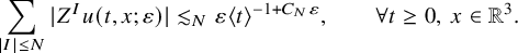 $$ \begin{align}\begin{aligned} \sum_{|I|\leq N}|Z^Iu(t,x;\varepsilon)|\lesssim_N \varepsilon \langle t \rangle^{-1+C_N\varepsilon},\qquad \forall t\geq 0,\ x\in\mathbb{R}^3. \end{aligned}\end{align} $$
There is a better bound for $\partial u$
:
$\partial u$
: $|\partial u|\lesssim \varepsilon \langle t \rangle ^{-1}$
. By the finite speed of propagation, we also have
$|\partial u|\lesssim \varepsilon \langle t \rangle ^{-1}$
. By the finite speed of propagation, we also have $u\equiv 0$
for
$u\equiv 0$
for $r-t\geq R$
.
$r-t\geq R$
.
3.2 The optical function
Fix a small parameter $\delta \in (0,1)$
. Define
$\delta \in (0,1)$
. Define
 $$ \begin{align}\begin{aligned} \Omega=\Omega_{\delta,R,\varepsilon}:=\{(t,x)\in(e^{\delta/\varepsilon},\infty)\times\mathbb{R}^3:\ |x|>\frac{1}{2}(t+e^{\delta/\varepsilon})+2R\}. \end{aligned}\end{align} $$
Heuristically, one can view $\Omega $
as
$\Omega $
as $\{t>e^{\delta /\varepsilon },\ |x|>t/2\}$
. Here, we use (3.2) for technical reasons; see the discussion below (3.3). From now on, if we use the notation
$\{t>e^{\delta /\varepsilon },\ |x|>t/2\}$
. Here, we use (3.2) for technical reasons; see the discussion below (3.3). From now on, if we use the notation $\varepsilon ^nS^{m,p}$
or
$\varepsilon ^nS^{m,p}$
or $\varepsilon ^nS^{m,p}_{\ln }$
, we always take
$\varepsilon ^nS^{m,p}_{\ln }$
, we always take $\mathcal {D}_{\varepsilon }=\Omega _{\delta ,R,\varepsilon }\cap \{r-t<2R\}$
in Definition 2.5. Thus, by (3.1), we have
$\mathcal {D}_{\varepsilon }=\Omega _{\delta ,R,\varepsilon }\cap \{r-t<2R\}$
in Definition 2.5. Thus, by (3.1), we have $u\in \varepsilon S^{-1,0}$
.
$u\in \varepsilon S^{-1,0}$
.
In [Reference Yu75, Propositions 3.1 and 4.1], we applied the method of characteristics and proved that the eikonal equation
 $$ \begin{align}\begin{aligned} g^{\alpha\beta}(u)\partial_\alpha q\partial_\beta q=0\quad\text{in }\Omega;\qquad q=|x|-t\quad \text{on }\partial\Omega \end{aligned}\end{align} $$
admits a unique global $C^2$
solution
$C^2$
solution $q=q(t,x;\varepsilon )$
in
$q=q(t,x;\varepsilon )$
in $\Omega $
. Because
$\Omega $
. Because $\partial \Omega $
is not a smooth surface, it seems that we need to carefully choose the boundary condition near the ‘corner’ of
$\partial \Omega $
is not a smooth surface, it seems that we need to carefully choose the boundary condition near the ‘corner’ of $\partial \Omega $
 $$ \begin{align*} \{t=e^{\delta/\varepsilon},|x|=e^{\delta/\varepsilon}+2R\}\subset\partial\Omega \end{align*} $$
to make q a $C^2$
solution. However, it is not necessary here because of our choice (3.2) of
$C^2$
solution. However, it is not necessary here because of our choice (3.2) of $\Omega $
. We have
$\Omega $
. We have $u|_{r-t\geq R}\equiv 0$
and
$u|_{r-t\geq R}\equiv 0$
and $q|_{r-t\geq R}=r-t$
, so we only need to consider those characteristics emanating from a smooth subset of
$q|_{r-t\geq R}=r-t$
, so we only need to consider those characteristics emanating from a smooth subset of $\partial \Omega $
(i.e.,
$\partial \Omega $
(i.e., $\partial \Omega \cap \{t>e^{\delta /\varepsilon }\}$
). Besides, we have
$\partial \Omega \cap \{t>e^{\delta /\varepsilon }\}$
). Besides, we have $q\in S^{0,1}$
and
$q\in S^{0,1}$
and $\langle r-t \rangle \lesssim \langle q \rangle t^{C\varepsilon }$
in
$\langle r-t \rangle \lesssim \langle q \rangle t^{C\varepsilon }$
in $\Omega $
, so we can take
$\Omega $
, so we can take $\rho =q$
in Lemma 2.7. To see this, we apply [Reference Yu75, Lemma 3.8] to obtain
$\rho =q$
in Lemma 2.7. To see this, we apply [Reference Yu75, Lemma 3.8] to obtain $|q-(r-t)|\lesssim t^{C\varepsilon }$
and
$|q-(r-t)|\lesssim t^{C\varepsilon }$
and $t^{-C\varepsilon }\lesssim \langle q \rangle /\langle r-t \rangle \lesssim t^{C\varepsilon }$
in
$t^{-C\varepsilon }\lesssim \langle q \rangle /\langle r-t \rangle \lesssim t^{C\varepsilon }$
in $\Omega $
. Next, we apply [Reference Yu75, Proposition 4.1] to conclude that for each fixed integer
$\Omega $
. Next, we apply [Reference Yu75, Proposition 4.1] to conclude that for each fixed integer $N\geq 2$
, the
$N\geq 2$
, the $C^2$
solution q is
$C^2$
solution q is $C^N$
as long as
$C^N$
as long as $\varepsilon \ll _N1$
. We also have
$\varepsilon \ll _N1$
. We also have $\sum _{|I|\leq N}|Z^Iq|\lesssim \langle q \rangle t^{C\varepsilon }\lesssim \langle r-t \rangle t^{C\varepsilon }$
in
$\sum _{|I|\leq N}|Z^Iq|\lesssim \langle q \rangle t^{C\varepsilon }\lesssim \langle r-t \rangle t^{C\varepsilon }$
in $\Omega $
.
$\Omega $
.
Next, if we set
 $$ \begin{align}\begin{aligned} \Omega'&:=\{(s,q,\omega)\in[0,\infty)\times\mathbb{R}\times\mathbb{S}^2:\ q>\frac{1}{2}(1-e^{s/\varepsilon})e^{\delta/\varepsilon}+2R\}, \end{aligned}\end{align} $$
then the map
 $$ \begin{align*} \Omega\to\Omega':\ (t,x)\mapsto (\varepsilon\ln t-\delta,q(t,x;\varepsilon),x/|x|) \end{align*} $$
is bijective and has an inverse map. As a result, any function defined for all $(t,x)\in \Omega $
induces a function of
$(t,x)\in \Omega $
induces a function of $(s,q,\omega )$
. Again, for each fixed integer
$(s,q,\omega )$
. Again, for each fixed integer $N\geq 2$
, both the map
$N\geq 2$
, both the map $\Omega \to \Omega '$
and its inverse are
$\Omega \to \Omega '$
and its inverse are $C^N$
as long as
$C^N$
as long as $\varepsilon \ll _N1$
.
$\varepsilon \ll _N1$
.
3.3 The geometric reduced system
In $\Omega $
, we set
$\Omega $
, we set $(\mu ,U)(t,x;\varepsilon ):=(q_t-q_r,\varepsilon ^{-1}ru)(t,x;\varepsilon )$
and obtain an induced function
$(\mu ,U)(t,x;\varepsilon ):=(q_t-q_r,\varepsilon ^{-1}ru)(t,x;\varepsilon )$
and obtain an induced function $(\mu ,U)(s,q,\omega ;\varepsilon )$
in
$(\mu ,U)(s,q,\omega ;\varepsilon )$
in $\Omega '$
. In [Reference Yu75, Section 5], we proved that
$\Omega '$
. In [Reference Yu75, Section 5], we proved that $(\mu ,U)$
is an approximate solution to the geometric reduced system (1.14). In addition, the following three limits exist for all
$(\mu ,U)$
is an approximate solution to the geometric reduced system (1.14). In addition, the following three limits exist for all $(q,\omega )\in \mathbb {R}\times \mathbb {S}^2$
:
$(q,\omega )\in \mathbb {R}\times \mathbb {S}^2$
:
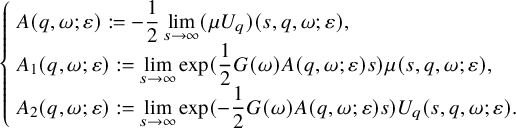 $$ \begin{align}\begin{aligned} \left\{\begin{array}{l} \displaystyle A(q,\omega;\varepsilon):=-\frac{1}{2}\lim_{s\to\infty}(\mu U_q)(s,q,\omega;\varepsilon),\\ \displaystyle A_1(q,\omega;\varepsilon):=\lim_{s\to\infty}\exp(\frac{1}{2}G(\omega)A(q,\omega;\varepsilon)s)\mu(s,q,\omega;\varepsilon),\\ \displaystyle A_2(q,\omega;\varepsilon):=\lim_{s\to\infty}\exp(-\frac{1}{2}G(\omega)A(q,\omega;\varepsilon)s)U_q(s,q,\omega;\varepsilon). \end{array}\right. \end{aligned}\end{align} $$
Note that $A_1A_2\equiv -2A$
. Since
$A_1A_2\equiv -2A$
. Since $u\equiv 0$
whenever
$u\equiv 0$
whenever $r\geq t+R$
, we have
$r\geq t+R$
, we have $(A,A_2)\equiv 0$
and
$(A,A_2)\equiv 0$
and $A_1\equiv -2$
for
$A_1\equiv -2$
for $q\geq R$
. By setting
$q\geq R$
. By setting
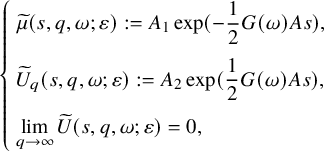 $$ \begin{align}\begin{aligned} \left\{\begin{array}{l} \displaystyle\widetilde{ \mu }(s,q,\omega;\varepsilon):=A_1\exp(-\frac{1}{2}G(\omega)As),\\[1em] \displaystyle \widetilde{ U }_q(s,q,\omega;\varepsilon):=A_2\exp(\frac{1}{2}G(\omega)As),\\[1em]\displaystyle \lim_{q\to\infty}\widetilde{ U }(s,q,\omega;\varepsilon)=0, \end{array}\right. \end{aligned}\end{align} $$
we obtain an exact solution $(\widetilde { \mu },\widetilde { U })$
to the reduced system (1.14). We refer our readers to [Reference Yu75, Proposition 5.1] for more details. Since
$(\widetilde { \mu },\widetilde { U })$
to the reduced system (1.14). We refer our readers to [Reference Yu75, Proposition 5.1] for more details. Since $A,A_1,A_2$
are defined for all
$A,A_1,A_2$
are defined for all $(q,\omega )\in \mathbb {R}\times \mathbb {S}^2$
, we emphasize that
$(q,\omega )\in \mathbb {R}\times \mathbb {S}^2$
, we emphasize that $(\widetilde { \mu },\widetilde { U })$
is defined for all
$(\widetilde { \mu },\widetilde { U })$
is defined for all $(s,q,\omega )\in \mathbb {R}\times \mathbb {R}\times \mathbb {S}^2$
. However,
$(s,q,\omega )\in \mathbb {R}\times \mathbb {R}\times \mathbb {S}^2$
. However, $(\mu ,U)$
is only defined in
$(\mu ,U)$
is only defined in $\Omega '$
.
$\Omega '$
.
In [Reference Yu75, Proposition 5.1], we also proved several bounds for $A,A_1,A_2$
in the coordinate set
$A,A_1,A_2$
in the coordinate set $(q,\omega )$
:
$(q,\omega )$
:
 $$ \begin{align}\begin{aligned} \partial_q^a\partial_\omega^c(A,A_2)=O_{a,c}(\langle q \rangle^{-1-a+C_{a,c}\varepsilon}),\quad \partial_q^a\partial_\omega^cA_1=O_{a,c}(\langle q \rangle^{-a+C_{a,c}\varepsilon}),\qquad \forall a,c\geq 0. \end{aligned}\end{align} $$
Here, we remind our readers of the convention introduced in Section 2.2. First, the estimates (3.7) should be understood in the following way: for each integer $N\geq 0$
, as long as
$N\geq 0$
, as long as $\varepsilon \ll _N1$
, the functions
$\varepsilon \ll _N1$
, the functions $A,A_1,A_2$
are
$A,A_1,A_2$
are $C^N$
and satisfy (3.7) for all
$C^N$
and satisfy (3.7) for all $a+c\leq N$
. Moreover, we emphasize that the constants in (3.7) can be chosen to be uniform for all
$a+c\leq N$
. Moreover, we emphasize that the constants in (3.7) can be chosen to be uniform for all $\varepsilon \ll _N1$
.
$\varepsilon \ll _N1$
.
In [Reference Yu75, Lemma 5.8], we proved that
 $$ \begin{align}\begin{aligned} |A_1+2|\leq \langle q \rangle^{-1+C\varepsilon},\qquad -3\leq A_1\leq -1<0. \end{aligned}\end{align} $$
Finally, we recall from [Reference Yu75, Proposition 5.1, (5.11), and (5.12)] that
 $$ \begin{align}\begin{aligned} \partial_q^a\partial_s^b\partial_\omega^c(\mu-\widetilde{ \mu })&=O_{a,b,c}(\varepsilon^{-b}\langle q \rangle^{-a}t^{-1+C_{a,b,c}\varepsilon}),\qquad &\forall a,b,c\geq 0,\ (s,q,\omega)\in\Omega';\\ \partial_q^a\partial_s^b\partial_\omega^c(U-\widetilde{ U })&=O_{a,b,c}(\varepsilon^{-b}\langle q \rangle^{1-a}t^{-1+C_{a,b,c}\varepsilon}),\qquad& \forall a,b,c\geq 0,\ (s,q,\omega)\in\Omega'; \end{aligned}\end{align} $$
 $$ \begin{align}\begin{aligned} \partial_q^a\partial_s^b\partial_\omega^c(\widetilde{ \mu },\widetilde{ U })&=O_{a,b,c}(\varepsilon^{-b}\langle q \rangle^{-a}t^{C_{a,b,c}\varepsilon}),\qquad &\forall a,b,c\geq 0,\ (s,q,\omega)\in\Omega'. \end{aligned}\end{align} $$
All the functions above are defined for $(s,q,\omega )\in \Omega '\subset [0,\infty )\times \mathbb {R}\times \mathbb {S}^2$
where
$(s,q,\omega )\in \Omega '\subset [0,\infty )\times \mathbb {R}\times \mathbb {S}^2$
where $\Omega '$
is defined by (3.4). Besides, we set
$\Omega '$
is defined by (3.4). Besides, we set $t=e^{\frac {s+\delta }{\varepsilon }}$
. Again, all the estimates above should be understood in the following way: for each integer
$t=e^{\frac {s+\delta }{\varepsilon }}$
. Again, all the estimates above should be understood in the following way: for each integer $N\geq 0$
, we can choose
$N\geq 0$
, we can choose $\varepsilon \ll _N1$
so that these estimates hold for all
$\varepsilon \ll _N1$
so that these estimates hold for all $a+b+c\leq N$
.
$a+b+c\leq N$
.
As discussed in Section 3.2, every function of $(s,q,\omega )$
induces a function of
$(s,q,\omega )$
induces a function of $(t,x)$
via the map
$(t,x)$
via the map $(t,x)\mapsto (\varepsilon \ln t-\delta ,q(t,x;\varepsilon ),x/|x|)$
. Below (3.3), we mentioned that
$(t,x)\mapsto (\varepsilon \ln t-\delta ,q(t,x;\varepsilon ),x/|x|)$
. Below (3.3), we mentioned that $q\in S^{0,1}$
and
$q\in S^{0,1}$
and $\langle r-t \rangle \lesssim \langle q \rangle t^{C\varepsilon }$
. Thus, we can apply Lemma 2.7 with
$\langle r-t \rangle \lesssim \langle q \rangle t^{C\varepsilon }$
. Thus, we can apply Lemma 2.7 with $\rho =q$
to obtain the following lemma.
$\rho =q$
to obtain the following lemma.
Lemma 3.1. We have $u-\varepsilon r^{-1}\widetilde { U }\in \varepsilon S^{-2,1}$
, and
$u-\varepsilon r^{-1}\widetilde { U }\in \varepsilon S^{-2,1}$
, and $\partial _\alpha u-\varepsilon \widehat { \omega }_\alpha r^{-1}A\in \varepsilon S^{-2,0}$
for
$\partial _\alpha u-\varepsilon \widehat { \omega }_\alpha r^{-1}A\in \varepsilon S^{-2,0}$
for $\alpha =0,1,2,3$
. Here,
$\alpha =0,1,2,3$
. Here, $\widehat { \omega }_0=-1$
and
$\widehat { \omega }_0=-1$
and $\widehat { \omega }_j=\omega _j$
for
$\widehat { \omega }_j=\omega _j$
for $j=1,2,3$
. That is, for each fixed integer
$j=1,2,3$
. That is, for each fixed integer $N\geq 0$
, as long as
$N\geq 0$
, as long as $\varepsilon \ll _N1$
, we have
$\varepsilon \ll _N1$
, we have
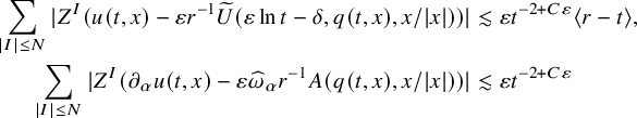 $$ \begin{align*} \sum_{|I|\leq N}|Z^I(u(t,x)-\varepsilon r^{-1}\widetilde{ U }(\varepsilon\ln t-\delta,q(t,x),x/|x|))|&\lesssim \varepsilon t^{-2+C\varepsilon}\langle r-t \rangle,\\ \sum_{|I|\leq N}|Z^I(\partial_\alpha u(t,x)-\varepsilon \widehat{ \omega }_\alpha r^{-1}A(q(t,x),x/|x|))|&\lesssim \varepsilon t^{-2+C\varepsilon} \end{align*} $$
for all $(t,x)\in \Omega $
. Note that the estimates hold trivially when
$(t,x)\in \Omega $
. Note that the estimates hold trivially when $r-t\geq R$
since
$r-t\geq R$
since $u,\widetilde { U },A$
vanish there.
$u,\widetilde { U },A$
vanish there.
Proof. We apply Lemma 2.7 with $\rho =q$
,
$\rho =q$
, $G=U-\widetilde { U }$
, and
$G=U-\widetilde { U }$
, and $(n,m,p)=(0,-1,1)$
. Thus, we have
$(n,m,p)=(0,-1,1)$
. Thus, we have $U-\widetilde { U }\in \ S^{-1,1}$
. By Lemma 2.6, we have
$U-\widetilde { U }\in \ S^{-1,1}$
. By Lemma 2.6, we have $\varepsilon r^{-1}\in \varepsilon S^{-1,0}$
and thus
$\varepsilon r^{-1}\in \varepsilon S^{-1,0}$
and thus $u-\varepsilon r^{-1}\widetilde { U }=\varepsilon r^{-1}(U-\widetilde { U })\in \varepsilon S^{-1,0}\cdot S^{-1,1}\subset \varepsilon S^{-2,1}$
.
$u-\varepsilon r^{-1}\widetilde { U }=\varepsilon r^{-1}(U-\widetilde { U })\in \varepsilon S^{-1,0}\cdot S^{-1,1}\subset \varepsilon S^{-2,1}$
.
Next, by part (d) of Lemma 2.6, we have $\partial _{\alpha }(u-\varepsilon r^{-1}\widetilde { U })\in \varepsilon S^{-2,0}$
. It suffices to prove that
$\partial _{\alpha }(u-\varepsilon r^{-1}\widetilde { U })\in \varepsilon S^{-2,0}$
. It suffices to prove that $\partial _{\alpha }(\varepsilon r^{-1}\widetilde { U })-\varepsilon \widehat { \omega }_\alpha r^{-1}A\in \varepsilon S^{-2,0}$
. By the chain rule and since
$\partial _{\alpha }(\varepsilon r^{-1}\widetilde { U })-\varepsilon \widehat { \omega }_\alpha r^{-1}A\in \varepsilon S^{-2,0}$
. By the chain rule and since $A=-\frac {1}{2}\widetilde { \mu }\widetilde { U }_q$
, we have
$A=-\frac {1}{2}\widetilde { \mu }\widetilde { U }_q$
, we have
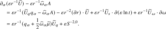 $$ \begin{align*} &\partial_\alpha(\varepsilon r^{-1}\widetilde{ U })-\varepsilon r^{-1}\widehat{ \omega }_\alpha A\\& \quad =\varepsilon r^{-1}(\widetilde{ U }_qq_\alpha-\widehat{ \omega }_\alpha A)-\varepsilon r^{-2}(\partial r)\cdot \widetilde{ U }+\varepsilon r^{-1}\widetilde{ U }_s\cdot\partial(\varepsilon\ln t)+\varepsilon r^{-1}\widetilde{ U }_{\omega}\cdot\partial\omega\\& \quad =\varepsilon r^{-1}(q_\alpha+\frac{1}{2}\widehat{ \omega }_\alpha \widetilde{ \mu })\widetilde{ U }_q+\varepsilon S^{-2,0}. \end{align*} $$
To obtain the last estimate, we first apply (3.10) and Lemma 2.7 to obtain $\widetilde { U },\widetilde { U }_\omega \in S^{0,0}$
and
$\widetilde { U },\widetilde { U }_\omega \in S^{0,0}$
and $\widetilde { U }_s\in \varepsilon ^{-1}S^{0,0}$
. By Lemma 2.6, we have
$\widetilde { U }_s\in \varepsilon ^{-1}S^{0,0}$
. By Lemma 2.6, we have $\varepsilon r^{-2}\partial r,\varepsilon r^{-1}\partial \omega \in \varepsilon S^{-2,0}$
and
$\varepsilon r^{-2}\partial r,\varepsilon r^{-1}\partial \omega \in \varepsilon S^{-2,0}$
and $\varepsilon r^{-1}\partial (\varepsilon \ln t)\in \varepsilon ^2S^{-2,0}$
.
$\varepsilon r^{-1}\partial (\varepsilon \ln t)\in \varepsilon ^2S^{-2,0}$
.
Finally, we need to show $\varepsilon r^{-1}(q_\alpha +\frac {1}{2}\widehat { \omega }_\alpha \widetilde { \mu })\widetilde { U }_q\in \varepsilon S^{2,0}$
. We have
$\varepsilon r^{-1}(q_\alpha +\frac {1}{2}\widehat { \omega }_\alpha \widetilde { \mu })\widetilde { U }_q\in \varepsilon S^{2,0}$
. We have $\varepsilon r^{-1}\in \varepsilon S^{-1,0}$
and
$\varepsilon r^{-1}\in \varepsilon S^{-1,0}$
and $\widetilde { U }_q\in S^{0,-1}$
by (3.10) and Lemma 2.7. Moreover, we have
$\widetilde { U }_q\in S^{0,-1}$
by (3.10) and Lemma 2.7. Moreover, we have
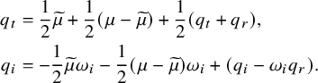 $$ \begin{align*} q_t&=\frac{1}{2}\widetilde{ \mu }+\frac{1}{2}(\mu-\widetilde{ \mu })+\frac{1}{2}(q_t+q_r),\\ q_i&=-\frac{1}{2}\widetilde{ \mu }\omega_i-\frac{1}{2}(\mu-\widetilde{ \mu })\omega_i+(q_i-\omega_iq_r). \end{align*} $$
By (3.9) and Lemma 2.7, we have $\mu -\widetilde { \mu }\in S^{-1,0}$
. Since
$\mu -\widetilde { \mu }\in S^{-1,0}$
. Since $q\in S^{0,1}$
, we apply part (d) of Lemma 2.6 to obtain
$q\in S^{0,1}$
, we apply part (d) of Lemma 2.6 to obtain $q_t+q_r,q_i-\omega _iq_r\in S^{-1,1}$
. As a result, we have
$q_t+q_r,q_i-\omega _iq_r\in S^{-1,1}$
. As a result, we have $q_\alpha +\frac {1}{2}\widetilde { \mu }\widehat { \omega }_\alpha \in S^{-1,1}$
. In summary, we have
$q_\alpha +\frac {1}{2}\widetilde { \mu }\widehat { \omega }_\alpha \in S^{-1,1}$
. In summary, we have
 $$ \begin{align*} \varepsilon r^{-1}(q_\alpha+\frac{1}{2}\widehat{ \omega }_\alpha \widetilde{ \mu })\widetilde{ U }_q\in \varepsilon S^{-1,0}\cdot S^{-1,1}\cdot S^{0,-1}\subset \varepsilon S^{-2,0}.\\[-41pt] \end{align*} $$
3.4 Approximation
In [Reference Yu75, Section 7], we used the limits in (3.5) to generate an approximate solution to (1.1) that is sufficiently close to the exact solution u in some sense. The construction is as follows. Recall from (3.6) that we have an exact solution $(\widetilde { \mu },\widetilde { U })(s,q,\omega ;\varepsilon )$
to the geometric reduced system (1.14). Now, we define a new function
$(\widetilde { \mu },\widetilde { U })(s,q,\omega ;\varepsilon )$
to the geometric reduced system (1.14). Now, we define a new function $\widetilde { q }=\widetilde { q }(t,x;\varepsilon )$
in
$\widetilde { q }=\widetilde { q }(t,x;\varepsilon )$
in $\Omega $
by solving
$\Omega $
by solving
 $$ \begin{align}\begin{aligned} \widetilde{ q }_t-\widetilde{ q }_r=\widetilde{ \mu }(\varepsilon\ln t-\delta,\widetilde{ q }(t,x;\varepsilon),x/|x|;\varepsilon)\quad\text{in }\Omega;\qquad \widetilde{ q }=|x|-t\text{ for }|x|-t\geq 2R. \end{aligned}\end{align} $$
We then define
 $$ \begin{align}\begin{aligned} \widetilde{ u }(t,x;\varepsilon)&=\varepsilon |x|^{-1}\widetilde{ U }(\varepsilon\ln t-\delta,\widetilde{ q }(t,x;\varepsilon),x/|x|;\varepsilon),\qquad \forall (t,x)\in\Omega. \end{aligned}\end{align} $$
Once again, both $\widetilde { q }$
and
$\widetilde { q }$
and $\widetilde { u }$
are
$\widetilde { u }$
are $C^N$
as long as
$C^N$
as long as $\varepsilon \ll _N1$
. In [Reference Yu75, Proposition 7.1 and Lemma 7.7], we proved that this
$\varepsilon \ll _N1$
. In [Reference Yu75, Proposition 7.1 and Lemma 7.7], we proved that this $\widetilde { u }$
is an approximate solution to (1.1), that for each integer
$\widetilde { u }$
is an approximate solution to (1.1), that for each integer $N\geq 0$
, as long as
$N\geq 0$
, as long as $\varepsilon \ll _N1$
,
$\varepsilon \ll _N1$
,
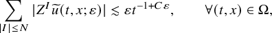 $$ \begin{align}\begin{aligned} \sum_{|I|\leq N}|Z^I\widetilde{ u }(t,x;\varepsilon)|\lesssim \varepsilon t^{-1+C\varepsilon},\qquad \forall (t,x)\in\Omega, \end{aligned}\end{align} $$
and that for each $\gamma \in (0,1)$
and each integer
$\gamma \in (0,1)$
and each integer $N\geq 0$
, as long as
$N\geq 0$
, as long as $\varepsilon \ll _{\gamma ,N}1$
,
$\varepsilon \ll _{\gamma ,N}1$
,
 $$ \begin{align}\begin{aligned} \sum_{|I|\leq N}|Z^I(u-\widetilde{ u })(t,x;\varepsilon)|\lesssim_{\gamma,N}\varepsilon t^{-2+C_N\varepsilon}\langle r-t \rangle,\qquad \forall (t,x)\in\Omega\cap\{|r-t|\lesssim t^\gamma\}. \end{aligned}\end{align} $$
We ask our readers to compare (3.14) with Lemma 3.1. First, the estimates (3.14) hold in $\Omega \cap \{|r-t|\lesssim t^\gamma \}$
, and the implicit constants depend on
$\Omega \cap \{|r-t|\lesssim t^\gamma \}$
, and the implicit constants depend on $\gamma $
. From this point of view, the estimates in Lemma 3.1 are better since they hold in
$\gamma $
. From this point of view, the estimates in Lemma 3.1 are better since they hold in $\Omega $
. However, we can construct
$\Omega $
. However, we can construct $\widetilde { u }$
from the functions
$\widetilde { u }$
from the functions $A,A_1,A_2$
without knowing what the exact solution u to (1.1) and the exact optical function q are. Recall that we construct an approximate optical function
$A,A_1,A_2$
without knowing what the exact solution u to (1.1) and the exact optical function q are. Recall that we construct an approximate optical function $\widetilde { q }$
by solving a transport equation which does not depend on u and q. However, to apply Lemma 3.1, we need the exact optical function q which is determined by the eikonal equation (3.3) involving u.
$\widetilde { q }$
by solving a transport equation which does not depend on u and q. However, to apply Lemma 3.1, we need the exact optical function q which is determined by the eikonal equation (3.3) involving u.
Here, we recall an alternative way to define $\widetilde { u }$
from [Reference Yu75, Section 7.2] which will simplify our computations. DefineFootnote
13
$\widetilde { u }$
from [Reference Yu75, Section 7.2] which will simplify our computations. DefineFootnote
13
 $$ \begin{align}\begin{aligned} F(q,\omega;\varepsilon):=2R-\int_{2R}^q \frac{2}{A_1(p,\omega;\varepsilon)}\ dp,\qquad\forall (q,\omega)\in\mathbb{R}\times\mathbb{S}^2. \end{aligned}\end{align} $$
Recall that $A_1\in [-3,-1]$
everywhere, so F is well defined. In [Reference Yu75, Section 7.2], we proved that
$A_1\in [-3,-1]$
everywhere, so F is well defined. In [Reference Yu75, Section 7.2], we proved that $\langle F(q,\omega ;\varepsilon ) \rangle \sim \langle q \rangle $
for all
$\langle F(q,\omega ;\varepsilon ) \rangle \sim \langle q \rangle $
for all $(q,\omega )\in \mathbb {R}\times \mathbb {S}^2$
. For each fixed
$(q,\omega )\in \mathbb {R}\times \mathbb {S}^2$
. For each fixed $\omega \in \mathbb {S}^2$
, the map
$\omega \in \mathbb {S}^2$
, the map $q\mapsto F(q,\omega ;\varepsilon )$
has an inverse
$q\mapsto F(q,\omega ;\varepsilon )$
has an inverse $\widehat { F }(q,\omega ;\varepsilon )$
. Set
$\widehat { F }(q,\omega ;\varepsilon )$
. Set
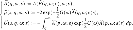 $$ \begin{align}\begin{aligned} \left\{\begin{array}{l} \displaystyle \widehat{ A }(q,\omega;\varepsilon):=A(\widehat{ F }(q,\omega;\varepsilon),\omega;\varepsilon),\\ \displaystyle \widehat{ \mu }(s,q,\omega;\varepsilon):=-2\exp(-\frac{1}{2}G(\omega)\widehat{ A }(q,\omega;\varepsilon)s),\\ \displaystyle \widehat{ U }(s,q,\omega;\varepsilon):=-\int_q^\infty \widehat{ A }(p,\omega;\varepsilon)\exp(\frac{1}{2}G(\omega)\widehat{ A }(p,\omega;\varepsilon)s) \ dp.\end{array}\right. \end{aligned}\end{align} $$
This $\widehat { A }$
is called the scattering data for the asymptotic completeness problem. Note that
$\widehat { A }$
is called the scattering data for the asymptotic completeness problem. Note that $(\widehat { \mu },\widehat { U })$
is again a solution to the geometric reduced system (1.14).
$(\widehat { \mu },\widehat { U })$
is again a solution to the geometric reduced system (1.14).
We summarize several estimates for $\widehat { A },\widehat { \mu },\widehat { U }$
in the next lemma. We again remind our readers of the convention in Section 2.2.
$\widehat { A },\widehat { \mu },\widehat { U }$
in the next lemma. We again remind our readers of the convention in Section 2.2.
Lemma 3.2. For all $a,c\geq 0$
, we have
$a,c\geq 0$
, we have
 $$ \begin{align}\begin{aligned} \partial_q^a\partial_\omega^c\widehat{ A }=O_{a,c}(\langle q \rangle^{-1-a+C_{a,c}\varepsilon}),\qquad \forall (q,\omega)\in\mathbb{R}\times\mathbb{S}^2. \end{aligned}\end{align} $$
For all $a,b,c\geq 0$
, we have
$a,b,c\geq 0$
, we have
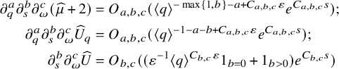 $$ \begin{align}\begin{aligned} \partial_q^a\partial_s^b\partial_\omega^c(\widehat{ \mu }+2)&=O_{a,b,c}(\langle q \rangle^{-\max\{1,b\}-a+C_{a,b,c}\varepsilon}e^{C_{a,b,c}s});\\ \partial_q^a\partial_s^b \partial_\omega^c\widehat{ U }_q&=O_{a,b,c}(\langle q \rangle^{-1-a-b+C_{a,b,c}\varepsilon}e^{C_{a,b,c}s});\\ \partial_s^b \partial_\omega^c\widehat{ U }&=O_{b,c}((\varepsilon^{-1}\langle q \rangle^{C_{b,c}\varepsilon}1_{b=0}+1_{b>0})e^{C_{b,c}s}) \end{aligned}\end{align} $$
for all $(s,q,\omega )\in [0,\infty )\times \mathbb {R}\times \mathbb {S}^2$
. Finally, for all
$(s,q,\omega )\in [0,\infty )\times \mathbb {R}\times \mathbb {S}^2$
. Finally, for all $c\geq 0$
,
$c\geq 0$
, $s\geq 0$
,
$s\geq 0$
, $\omega \in \mathbb {S}^2$
, and
$\omega \in \mathbb {S}^2$
, and $q>C_0e^{C_0s}(e^{\delta /\varepsilon }-e^{(\delta +s)/\varepsilon }-1)$
for some constant
$q>C_0e^{C_0s}(e^{\delta /\varepsilon }-e^{(\delta +s)/\varepsilon }-1)$
for some constant $C_0>1$
, we have
$C_0>1$
, we have
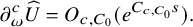 $$ \begin{align}\begin{aligned} \partial_\omega^c\widehat{ U }&=O_{c,C_0}(e^{C_{c,C_0}s}). \end{aligned}\end{align} $$
Proof. The estimates (3.17) have been proved in [Reference Yu75, Proposition 7.3]. We now prove (3.18) for all $(s,q,\omega )\in [0,\infty )\times \mathbb {R}\times \mathbb {S}^2$
. Since
$(s,q,\omega )\in [0,\infty )\times \mathbb {R}\times \mathbb {S}^2$
. Since $|e^x-1|\leq |x|e^{|x|}$
, we have
$|e^x-1|\leq |x|e^{|x|}$
, we have $|\widehat { \mu }+2|\lesssim |G(\omega )\widehat { A }s|e^{Cs}\lesssim \langle q \rangle ^{-1+C\varepsilon }e^{Cs}$
. Next, for
$|\widehat { \mu }+2|\lesssim |G(\omega )\widehat { A }s|e^{Cs}\lesssim \langle q \rangle ^{-1+C\varepsilon }e^{Cs}$
. Next, for $a+c>0$
, we write
$a+c>0$
, we write $\partial _q^a\partial _\omega ^c\widehat { \mu }$
as a linear combination (with real constant coefficients depending only on a and c) of terms of the form
$\partial _q^a\partial _\omega ^c\widehat { \mu }$
as a linear combination (with real constant coefficients depending only on a and c) of terms of the form
 $$ \begin{align*} \exp(-\frac{1}{2}G \widehat{ A }s)\cdot\prod_{j=1}^k \partial_q^{a_j}\partial_\omega^{c_j}(-\frac{1}{2}G \widehat{ A }s),\qquad \sum a_*=a,\ \sum c_*=c,\ a_j+c_j>0\text{ for each }j. \end{align*} $$
The estimates for $\widehat { A }$
imply that
$\widehat { A }$
imply that
 $$ \begin{align*} |\exp(-\frac{1}{2}G \widehat{ A }s)\cdot\prod_{j=1}^k \partial_q^{a_j}\partial_\omega^{c_j}(-\frac{1}{2}G \widehat{ A }s)|\lesssim e^{Cs}\cdot \langle q \rangle^{-1-\sum a_j+C\varepsilon}s^k\lesssim \langle q \rangle^{-1-a+C\varepsilon}e^{Cs}. \end{align*} $$
In summary, we have $|\partial _q^a\partial _\omega ^c\widehat { \mu }|\lesssim _{a,c} \langle q \rangle ^{-1-a+C_{a,c}\varepsilon }e^{C_{a,c}s}$
. That is, we obtain the first estimate in (3.18) with
$|\partial _q^a\partial _\omega ^c\widehat { \mu }|\lesssim _{a,c} \langle q \rangle ^{-1-a+C_{a,c}\varepsilon }e^{C_{a,c}s}$
. That is, we obtain the first estimate in (3.18) with $b=0$
.
$b=0$
.
Now, by (3.16), we notice that
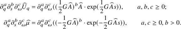 $$ \begin{align}\begin{aligned} \partial_q^a\partial_s^b\partial_\omega^c\widehat{ U }_q&=\partial_q^a\partial_\omega^c((\frac{1}{2}G\widehat{ A })^b\widehat{ A }\cdot\exp(\frac{1}{2}G\widehat{ A }s)),\qquad a,b,c\geq 0;\\ \partial_q^a\partial_s^b\partial_\omega^c\widehat{ \mu }&=\partial_q^a\partial_\omega^c((-\frac{1}{2}G\widehat{ A })^b\cdot\exp(-\frac{1}{2}G\widehat{ A }s)),\qquad a,c\geq 0,b>0. \end{aligned}\end{align} $$
Both of these rows are of the form
 $$ \begin{align*} \partial_q^a\partial_\omega^c[F_1(q,\omega)\cdot \exp(F_2(q,\omega)s)]. \end{align*} $$
Here, for all $a,c\geq 0$
and
$a,c\geq 0$
and $j=1,2$
, we have
$j=1,2$
, we have $\partial _q^a\partial _\omega ^cF_j=O_{a,c}(\langle q \rangle ^{-b_j+C_{a,c}\varepsilon })$
for some fixed constants
$\partial _q^a\partial _\omega ^cF_j=O_{a,c}(\langle q \rangle ^{-b_j+C_{a,c}\varepsilon })$
for some fixed constants $b_1>0$
and
$b_1>0$
and $b_2=1$
. Following the same proof in the previous paragraph for
$b_2=1$
. Following the same proof in the previous paragraph for $\widehat { \mu }$
, we obtain that for all
$\widehat { \mu }$
, we obtain that for all $a,c\geq 0$
and
$a,c\geq 0$
and $(s,q,\omega )$
,
$(s,q,\omega )$
,
 $$ \begin{align*} \partial_q^a\partial_\omega^c(\exp(F_2(q,\omega)s)-1)=O_{a,c}(\langle q \rangle^{-1-a+C_{a,c}\varepsilon}e^{C_{a,c}s}). \end{align*} $$
Thus, by Leibniz’s rule, for all $a,c\geq 0$
and
$a,c\geq 0$
and $(s,q,\omega )$
, we have
$(s,q,\omega )$
, we have
 $$ \begin{align*} &\partial_q^a\partial_\omega^c[F_1(q,\omega)\cdot \exp(F_2(q,\omega)s)]=\partial_q^a\partial_\omega^cF_1+\partial_q^a\partial_\omega^c[F_1 \cdot (\exp(F_2 s)-1)]\\&\quad =O_{a,c}(\langle q \rangle^{-b_1-a+C_{a,c}\varepsilon}e^{C_{a,c}s}+\langle q \rangle^{-b_1-1-a+C_{a,c}\varepsilon}e^{C_{a,c}s})=O_{a,c}(\langle q \rangle^{-b_1-a+C_{a,c}\varepsilon}e^{C_{a,c}s}). \end{align*} $$
To estimate the derivatives of $\widehat { U }_q$
, we use (3.20) to set
$\widehat { U }_q$
, we use (3.20) to set $F_1=(\frac {1}{2}G\widehat { A })^b\widehat { A }$
and
$F_1=(\frac {1}{2}G\widehat { A })^b\widehat { A }$
and $F_2=\frac {1}{2}G\widehat { A }$
. In this case, we have
$F_2=\frac {1}{2}G\widehat { A }$
. In this case, we have $b_1=b+1$
, so we obtain the second row of (3.18). To estimate the derivatives of
$b_1=b+1$
, so we obtain the second row of (3.18). To estimate the derivatives of $\widehat { \mu }$
, we use (3.20) to set
$\widehat { \mu }$
, we use (3.20) to set $F_1=(\frac {1}{2}G\widehat { A })^b$
and
$F_1=(\frac {1}{2}G\widehat { A })^b$
and $F_2=-\frac {1}{2}G\widehat { A }$
. In this case, we have
$F_2=-\frac {1}{2}G\widehat { A }$
. In this case, we have $b_1=b$
, so we obtain the first row of (3.18) with
$b_1=b$
, so we obtain the first row of (3.18) with $b>0$
.
$b>0$
.
To end the proof of (3.18), we prove the bounds for $\partial _s^b\partial _\omega ^c\widehat { U }$
. Note that
$\partial _s^b\partial _\omega ^c\widehat { U }$
. Note that $\widehat { U }\equiv 0$
for
$\widehat { U }\equiv 0$
for $q\geq R$
and that for
$q\geq R$
and that for $q<R$
,
$q<R$
,
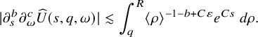 $$ \begin{align*} |\partial_s^b\partial_\omega^c\widehat{ U }(s,q,\omega)|&\lesssim \int_{q}^R \langle \rho \rangle^{-1-b+C\varepsilon}e^{Cs}\ d\rho. \end{align*} $$
When $b=0$
, the right side is
$b=0$
, the right side is $O(\varepsilon ^{-1}\langle q \rangle ^{C\varepsilon }e^{Cs})$
. If
$O(\varepsilon ^{-1}\langle q \rangle ^{C\varepsilon }e^{Cs})$
. If $b\geq 1$
, the right side is
$b\geq 1$
, the right side is $O(e^{Cs})$
.
$O(e^{Cs})$
.
Finally, we check (3.19). Recall from [Reference Yu75, Proposition 7.3] that $\partial _\omega ^c\widehat { U }=O(e^{Cs})$
for
$\partial _\omega ^c\widehat { U }=O(e^{Cs})$
for $(s,q,\omega )\in \Omega '$
. That is,
$(s,q,\omega )\in \Omega '$
. That is, $(s,\omega )\in [0,\infty )\times \mathbb {S}^2$
and
$(s,\omega )\in [0,\infty )\times \mathbb {S}^2$
and $q>q_{(s,\varepsilon )}:=\frac {1}{2}(e^{\delta /\varepsilon }-e^{(s+\delta )/\varepsilon })+2R$
. Since
$q>q_{(s,\varepsilon )}:=\frac {1}{2}(e^{\delta /\varepsilon }-e^{(s+\delta )/\varepsilon })+2R$
. Since $e^{\delta /\varepsilon }-e^{(\delta +s)/\varepsilon }-1=2q_{(s,\varepsilon )}-4R-1<0$
and since
$e^{\delta /\varepsilon }-e^{(\delta +s)/\varepsilon }-1=2q_{(s,\varepsilon )}-4R-1<0$
and since $q_{(s,\varepsilon )}\leq 2R$
, we have
$q_{(s,\varepsilon )}\leq 2R$
, we have
 $$ \begin{align*} \langle q \rangle/\langle q_{(s,\varepsilon)} \rangle+\langle q_{(s,\varepsilon)} \rangle/\langle q \rangle\lesssim_{R,C_0}e^{C_0s},\qquad \text{whenever } C_0e^{C_0s}(e^{\delta/\varepsilon}-e^{(\delta+s)/\varepsilon}-1)<q\leq q_{(s,\varepsilon)}. \end{align*} $$
Since $\partial _\omega ^c\widehat { U }_q=O(\langle q \rangle ^{-1+C\varepsilon }e^{Cs})$
by (3.18), by the mean value theorem, we have
$\partial _\omega ^c\widehat { U }_q=O(\langle q \rangle ^{-1+C\varepsilon }e^{Cs})$
by (3.18), by the mean value theorem, we have
 $$ \begin{align*} \partial_\omega^c\widehat{ U }(s,q,\omega;\varepsilon)&=\partial_\omega^c\widehat{ U }(s,q_{(s,\varepsilon)},\omega;\varepsilon)+O(|q-q_{(s,\varepsilon)}|\cdot \langle q_{(s,\varepsilon)} \rangle^{-1+C\varepsilon}e^{Cs})\\ &=O(e^{Cs})+O(\langle q_{(s,\varepsilon)} \rangle\cdot \langle q_{(s,\varepsilon)} \rangle^{-1+C\varepsilon}\cdot e^{Cs})=O(e^{Cs}) \end{align*} $$
for all $C_0e^{C_0s}(e^{\delta /\varepsilon }-e^{(\delta +s)/\varepsilon }-1)<q\leq q_{(s,\varepsilon )}$
. This finishes the proof.
$C_0e^{C_0s}(e^{\delta /\varepsilon }-e^{(\delta +s)/\varepsilon }-1)<q\leq q_{(s,\varepsilon )}$
. This finishes the proof.
Remark 3.2.1. The bounds for $\widehat { \mu }$
in (3.18) are better than those for
$\widehat { \mu }$
in (3.18) are better than those for $\widetilde { \mu }$
. For example, we have
$\widetilde { \mu }$
. For example, we have $\widehat { \mu }_q=O(\langle q \rangle ^{-2+C\varepsilon }e^{Cs})$
but
$\widehat { \mu }_q=O(\langle q \rangle ^{-2+C\varepsilon }e^{Cs})$
but $\widetilde { \mu }_q=O(\langle q \rangle ^{-1+C\varepsilon }e^{Cs})$
. Such a difference occurs because we have
$\widetilde { \mu }_q=O(\langle q \rangle ^{-1+C\varepsilon }e^{Cs})$
. Such a difference occurs because we have $\partial _q(-2)=0$
and
$\partial _q(-2)=0$
and $\partial _qA_1=O(\langle q \rangle ^{-1+C\varepsilon })$
. This explains why we introduce this new map F.
$\partial _qA_1=O(\langle q \rangle ^{-1+C\varepsilon })$
. This explains why we introduce this new map F.
It follows from [Reference Yu75, Lemma 7.2] that $\widehat { q }(t,x;\varepsilon ):=F(\widetilde { q }(t,x;\varepsilon ),x/|x|;\varepsilon )$
solves
$\widehat { q }(t,x;\varepsilon ):=F(\widetilde { q }(t,x;\varepsilon ),x/|x|;\varepsilon )$
solves
 $$ \begin{align}\begin{aligned} \widehat{ q }_t-\widehat{ q }_r=\widehat{ \mu }(\varepsilon\ln t-\delta,\widehat{ q }(t,x;\varepsilon),x/|x|;\varepsilon),\qquad\text{in }\Omega, \end{aligned}\end{align} $$
that $\widehat { q }=r-t$
for
$\widehat { q }=r-t$
for $r-t\geq R$
, and that
$r-t\geq R$
, and that
 $$ \begin{align}\begin{aligned} \widetilde{ u }(t,x;\varepsilon)=\widehat{ u }(t,x;\varepsilon):=\varepsilon |x|^{-1}\widehat{ U }(\varepsilon\ln t-\delta,\widehat{ q }(t,x;\varepsilon),x/|x|;\varepsilon),\qquad\text{in }\Omega. \end{aligned}\end{align} $$
In the rest of this subsection, every function of $(s,q,\omega )$
induces a function of
$(s,q,\omega )$
induces a function of $(t,x)$
via the map
$(t,x)$
via the map $(t,x)\mapsto (\varepsilon \ln t-\delta ,\widehat { q }(t,x;\varepsilon ),x/|x|)$
. Note that this is different from the setting in Section 3.3. By [Reference Yu75, Lemmas 7.4 and 7.7], we have
$(t,x)\mapsto (\varepsilon \ln t-\delta ,\widehat { q }(t,x;\varepsilon ),x/|x|)$
. Note that this is different from the setting in Section 3.3. By [Reference Yu75, Lemmas 7.4 and 7.7], we have $\widehat { q }\in S^{0,1}$
and
$\widehat { q }\in S^{0,1}$
and $\langle r-t \rangle \lesssim \langle \widehat { q } \rangle t^{C\varepsilon }$
. Thus, we can apply Lemma 2.7 with
$\langle r-t \rangle \lesssim \langle \widehat { q } \rangle t^{C\varepsilon }$
. Thus, we can apply Lemma 2.7 with $\rho =\widehat { q }$
. For convenience, we list some results from (3.18) and (3.19):
$\rho =\widehat { q }$
. For convenience, we list some results from (3.18) and (3.19):
 $$ \begin{align}\begin{aligned} \widehat{ U },\varepsilon\widehat{ U }_s\in S^{0,0};\ \widehat{ u }=\varepsilon r^{-1}\widehat{ U }\in \varepsilon S^{-1,0};\ \widehat{ \mu }+2\in S^{0,-1}; \end{aligned}\end{align} $$
All the functions here are of $(t,x)$
via the map
$(t,x)$
via the map $(t,x)\mapsto (\varepsilon \ln t-\delta ,\widehat { q }(t,x;\varepsilon ),x/|x|)=(s,q,\omega )$
. We will use them in the next subsection. Note that
$(t,x)\mapsto (\varepsilon \ln t-\delta ,\widehat { q }(t,x;\varepsilon ),x/|x|)=(s,q,\omega )$
. We will use them in the next subsection. Note that $(t,x)\in \Omega $
does not imply that
$(t,x)\in \Omega $
does not imply that $(\varepsilon \ln t-\delta ,\widehat { q },x/|x|)\in \Omega '$
. Instead, by [Reference Yu75, Lemma 7.4], we have
$(\varepsilon \ln t-\delta ,\widehat { q },x/|x|)\in \Omega '$
. Instead, by [Reference Yu75, Lemma 7.4], we have $\langle \widehat { q } \rangle /\langle r-t \rangle +\langle r-t \rangle /\langle \widehat { q } \rangle \lesssim t^{C\varepsilon }$
in
$\langle \widehat { q } \rangle /\langle r-t \rangle +\langle r-t \rangle /\langle \widehat { q } \rangle \lesssim t^{C\varepsilon }$
in $\Omega $
. That is, in
$\Omega $
. That is, in $\Omega \cap \{r-t\leq 2R\}$
, we have
$\Omega \cap \{r-t\leq 2R\}$
, we have $\widehat { q }\leq 2R$
and
$\widehat { q }\leq 2R$
and
 $$ \begin{align*} 0<(2R+1-\widehat{ q })\sim\langle \widehat{ q } \rangle\lesssim\langle r-t \rangle t^{C\varepsilon}\lesssim (t-e^{\delta/\varepsilon}+1)t^{C\varepsilon}. \end{align*} $$
We hope that the estimate (3.19) holds for such a $\widehat { q }$
, so we assume
$\widehat { q }$
, so we assume $q>C_0e^{C_0s}(e^{\delta /\varepsilon }-e^{(\delta +s)/\varepsilon }-1)$
in Lemma 3.2.
$q>C_0e^{C_0s}(e^{\delta /\varepsilon }-e^{(\delta +s)/\varepsilon }-1)$
in Lemma 3.2.
3.5 Further computations
In the next proposition, we present asymptotic formulas for $Z^I\widehat { u }$
and
$Z^I\widehat { u }$
and $(\partial _t-\partial _r)Z^I\widehat { u }$
in
$(\partial _t-\partial _r)Z^I\widehat { u }$
in $\Omega $
. We remind our readers of the definitions of
$\Omega $
. We remind our readers of the definitions of $\varepsilon ^*S^{*,*}$
and
$\varepsilon ^*S^{*,*}$
and $\varepsilon ^*S^{*,*}_{\ln }$
in Definition 2.5.
$\varepsilon ^*S^{*,*}_{\ln }$
in Definition 2.5.
Proposition 3.3. For each multiindex I, there exist functions $U_I=U_I(s,q,\omega ;\varepsilon )$
and
$U_I=U_I(s,q,\omega ;\varepsilon )$
and $A_I=A_I(q,\omega ;\varepsilon )$
defined for all
$A_I=A_I(q,\omega ;\varepsilon )$
defined for all $(s,q,\omega )\in [0,\infty )\times \mathbb {R}\times \mathbb {S}^2$
and
$(s,q,\omega )\in [0,\infty )\times \mathbb {R}\times \mathbb {S}^2$
and $\varepsilon \ll _I1$
, such that
$\varepsilon \ll _I1$
, such that
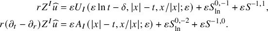 $$ \begin{align}\begin{aligned} r Z^I\widehat{ u }&=\varepsilon U_I(\varepsilon\ln t-\delta,|x|-t,x/|x|;\varepsilon)+\varepsilon S^{0,-1}_{\ln}+\varepsilon S^{-1,1},\\ r(\partial_t-\partial_r)Z^I\widehat{ u }&=\varepsilon A_I(|x|-t,x/|x|;\varepsilon)+\varepsilon S^{0,-2}_{\ln}+\varepsilon S^{-1,0}. \end{aligned} \end{align} $$
Here, $U_I$
and
$U_I$
and $A_I$
are defined inductively on
$A_I$
are defined inductively on $|I|$
. First, we have
$|I|$
. First, we have $U_0=\widehat { U }$
and
$U_0=\widehat { U }$
and $A_0=-2\widehat { A }$
. Moreover, for each
$A_0=-2\widehat { A }$
. Moreover, for each $|I|>0$
, by writing
$|I|>0$
, by writing $Z^I=ZZ^{I'}$
with
$Z^I=ZZ^{I'}$
with $|I'|=|I|-1$
, we define
$|I'|=|I|-1$
, we define $U_I$
and
$U_I$
and $A_I$
inductively by
$A_I$
inductively by
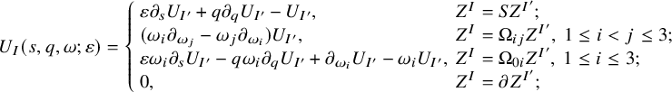 $$ \begin{align} U_I(s,q,\omega;\varepsilon)&=\left\{ \begin{array}{ll} \varepsilon\partial_sU_{I'}+q\partial_qU_{I'}-U_{I'}, & Z^I=SZ^{I'}; \\ (\omega_i\partial_{\omega_j}-\omega_j\partial_{\omega_i})U_{I'}, & Z^I=\Omega_{ij}Z^{I'},\ 1\leq i<j\leq 3;\\ \varepsilon\omega_i\partial_sU_{I'}-q\omega_i\partial_qU_{I'}+\partial_{\omega_i}U_{I'}-\omega_iU_{I'}, & Z^I=\Omega_{0i}Z^{I'},\ 1\leq i\leq 3;\\ 0, & Z^I=\partial Z^{I'}; \end{array}\right. \end{align} $$
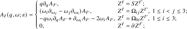 $$ \begin{align}A_I(q,\omega;\varepsilon)&=\left\{ \begin{array}{ll} q\partial_qA_{I'}, & Z^I=SZ^{I'}; \\ (\omega_i\partial_{\omega_j}-\omega_j\partial_{\omega_i})A_{I'}, & Z^I=\Omega_{ij}Z^{I'},\ 1\leq i<j\leq 3;\\ -q\omega_i\partial_qA_{I'}+\partial_{\omega_i}A_{I'}-2\omega_iA_{I'}, & Z^I=\Omega_{0i}Z^{I'},\ 1\leq i\leq 3;\\ 0, & Z^I=\partial Z^{I'}; \end{array}\right.\end{align} $$
Note that $\widehat { U }\equiv \widehat { A }\equiv 0$
for
$\widehat { U }\equiv \widehat { A }\equiv 0$
for $q\geq R$
, so by (3.25) and (3.26), we have
$q\geq R$
, so by (3.25) and (3.26), we have $U_I\equiv A_I\equiv 0$
for all
$U_I\equiv A_I\equiv 0$
for all $q\geq R$
. For all
$q\geq R$
. For all $a,b,c\geq 0$
, we have
$a,b,c\geq 0$
, we have
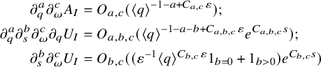 $$ \begin{align}\begin{aligned} \partial_q^a\partial_\omega^cA_I&=O_{a,c}(\langle q \rangle^{-1-a+C_{a,c}\varepsilon});\\ \partial_q^a\partial_s^b \partial_\omega^c\partial_qU_I&=O_{a,b,c}(\langle q \rangle^{-1-a-b+C_{a,b,c}\varepsilon}e^{C_{a,b,c}s});\\ \partial_s^b \partial_\omega^cU_I&=O_{b,c}((\varepsilon^{-1}\langle q \rangle^{C_{b,c}\varepsilon}1_{b=0}+1_{b>0})e^{C_{b,c}s}) \end{aligned}\end{align} $$
for all $(s,q,\omega )\in [0,\infty )\times \mathbb {R}\times \mathbb {S}^2$
. For all
$(s,q,\omega )\in [0,\infty )\times \mathbb {R}\times \mathbb {S}^2$
. For all $c\geq 0$
, we have
$c\geq 0$
, we have
 $$ \begin{align}\begin{aligned} \partial_\omega^cU_I=O_{c,C_0}(e^{C_{c,C_0}s}) \end{aligned}\end{align} $$
for all $s>0$
,
$s>0$
, $\omega \in \mathbb {S}^2$
, and
$\omega \in \mathbb {S}^2$
, and $q>C_0e^{C_0s}(e^{\delta /\varepsilon }-e^{(\delta +s)/\varepsilon }-1)$
for some constant
$q>C_0e^{C_0s}(e^{\delta /\varepsilon }-e^{(\delta +s)/\varepsilon }-1)$
for some constant $C_0>1$
. Finally, for all
$C_0>1$
. Finally, for all $a,b,c\geq 0$
, we have
$a,b,c\geq 0$
, we have
 $$ \begin{align}\begin{aligned} \partial_q^a\partial_s^b\partial_\omega^c(2\partial_qU_I+A_I)(s,q,\omega;\varepsilon) &=O_{a,b,c}(\langle q \rangle^{-\max\{1,b\}-1-a+C_{a,b,c}\varepsilon}e^{C_{a,b,c}s}) \end{aligned}\end{align} $$
for all $(s,q,\omega )\in [0,\infty )\times \mathbb {R}\times \mathbb {S}^2$
.
$(s,q,\omega )\in [0,\infty )\times \mathbb {R}\times \mathbb {S}^2$
.
Remark 3.3.1. Since $\widehat { u }=\varepsilon r^{-1}\widehat { U }(s,\widehat { q },\omega )$
is defined explicitly by (3.22), one can compute
$\widehat { u }=\varepsilon r^{-1}\widehat { U }(s,\widehat { q },\omega )$
is defined explicitly by (3.22), one can compute $Z^I\widehat { u }$
by the chain rule and Leibniz’s rule. This has been done in, for example, the proof of Lemma 2.7. Thus, we can obtain an identity for
$Z^I\widehat { u }$
by the chain rule and Leibniz’s rule. This has been done in, for example, the proof of Lemma 2.7. Thus, we can obtain an identity for $Z^I\widehat { u }$
. Similarly for
$Z^I\widehat { u }$
. Similarly for $(\partial _t-\partial _r)Z^I\widehat { u }$
. In this paper, we prefer the asymptotic formulas (3.24) over these identities because (3.24) are much simpler.
$(\partial _t-\partial _r)Z^I\widehat { u }$
. In this paper, we prefer the asymptotic formulas (3.24) over these identities because (3.24) are much simpler.
Let us compute $Z\widehat { u }$
as an example. It suffices to compute
$Z\widehat { u }$
as an example. It suffices to compute $Z(r\widehat { u })=Z(\varepsilon \widehat { U }(\varepsilon \ln t-\delta ,\widehat { q },\omega ))$
because of the commutator
$Z(r\widehat { u })=Z(\varepsilon \widehat { U }(\varepsilon \ln t-\delta ,\widehat { q },\omega ))$
because of the commutator $[Z,r]=Zr$
. By the chain rule, we obtain the following term in the expansion of
$[Z,r]=Zr$
. By the chain rule, we obtain the following term in the expansion of $Z(r\widehat { u })$
:
$Z(r\widehat { u })$
:
 $$ \begin{align}\begin{aligned} \varepsilon\widehat{ U }_q(\varepsilon\ln t-\delta,\widehat{ q },\omega)\cdot Z\widehat{ q }. \end{aligned}\end{align} $$
Recall that $\widehat { q }$
is a solution to the transport equation (3.21). There is no explicit formula for
$\widehat { q }$
is a solution to the transport equation (3.21). There is no explicit formula for $Z\widehat { q }$
, so we cannot further simplify (3.30). In Proposition 3.3, we use an alternative way. We first show that
$Z\widehat { q }$
, so we cannot further simplify (3.30). In Proposition 3.3, we use an alternative way. We first show that $Z(r\widehat { u })$
equals
$Z(r\widehat { u })$
equals $Z(\varepsilon \widehat { U }(\varepsilon \ln t-\delta ,r-t,\omega ))$
up to a remainder term. This remainder term is good because we expect
$Z(\varepsilon \widehat { U }(\varepsilon \ln t-\delta ,r-t,\omega ))$
up to a remainder term. This remainder term is good because we expect $\widehat { q }\approx r-t$
to some extent; see Lemma 3.4 below. By the chain rule, we replace (3.30) with
$\widehat { q }\approx r-t$
to some extent; see Lemma 3.4 below. By the chain rule, we replace (3.30) with
 $$ \begin{align*} \varepsilon\widehat{ U }_q(\varepsilon\ln t-\delta,r-t,\omega)\cdot Z(r-t). \end{align*} $$
We can compute this expression explicitly because we have $S(r-t)=r-t$
,
$S(r-t)=r-t$
, $\Omega _{0i}(r-t)=(t-r)\omega _i$
, and
$\Omega _{0i}(r-t)=(t-r)\omega _i$
, and $Z(r-t)=0$
for other Z. As a result, we obtain a simpler asymptotic formula for
$Z(r-t)=0$
for other Z. As a result, we obtain a simpler asymptotic formula for $Z\widehat { u }$
.
$Z\widehat { u }$
.
Remark 3.3.2. As commented in Remark 1.4, if $Z^I$
contains a translation, we have
$Z^I$
contains a translation, we have $A_I\equiv 0$
. In this case, we can still approximate
$A_I\equiv 0$
. In this case, we can still approximate $Z^I\widehat { u }$
. We achieve this goal by following Remark 1.4, and we remark that the key is the identity (1.25).
$Z^I\widehat { u }$
. We achieve this goal by following Remark 1.4, and we remark that the key is the identity (1.25).
The key step in the proof of Proposition 3.3 is to show the following estimates:
 $$ \begin{align}\begin{aligned} r\widehat{ u }-\varepsilon\widehat{ U }(\varepsilon\ln t-\delta,r-t,\omega;\varepsilon)&\in\varepsilon S^{0,-1}_{\ln}+\varepsilon S^{-1,1},\\ (\partial_t-\partial_r)(r\widehat{ u })+2\varepsilon\widehat{ A }(r-t,\omega;\varepsilon)&\in\varepsilon S^{0,-2}_{\ln}+\varepsilon S^{-1,0}. \end{aligned}\end{align} $$
Recall that $r=|x|$
and
$r=|x|$
and $\omega =x/|x|$
. Proving these estimates requires several estimates for the approximate optical function
$\omega =x/|x|$
. Proving these estimates requires several estimates for the approximate optical function $\widehat { q }$
; see Section 3.5.1.
$\widehat { q }$
; see Section 3.5.1.
In Section 3.5.2, we extend (3.31) by showing that for each multiindex I, we have
 $$ \begin{align}\begin{aligned} rZ^I\widehat{ u }&=\varepsilon U_I(\varepsilon\ln t-\delta,r-t,\omega;\varepsilon)+\varepsilon S^{0,-1}_{\ln}+\varepsilon S^{-1,1},\\(\partial_t-\partial_r)(rZ^I\widehat{ u })&=\varepsilon A_I(r-t,\omega;\varepsilon)+\varepsilon S^{0,-2}_{\ln}+\varepsilon S^{-1,0}. \end{aligned} \end{align} $$
Here, the $U_I$
and
$U_I$
and $A_I$
are defined in the statement of Proposition 3.3: we set
$A_I$
are defined in the statement of Proposition 3.3: we set $(U_0,A_0)=(\widehat { U },-2\widehat { A })$
and define
$(U_0,A_0)=(\widehat { U },-2\widehat { A })$
and define $(U_I,A_I)$
inductively by (3.25) and (3.26) for
$(U_I,A_I)$
inductively by (3.25) and (3.26) for $|I|>0$
. We can induct on
$|I|>0$
. We can induct on $|I|$
to check (3.27) and (3.28); the details of the proofs are omitted. We also notice that
$|I|$
to check (3.27) and (3.28); the details of the proofs are omitted. We also notice that $[\partial _t-\partial _r,r]Z^I\widehat { u }=-Z^I\widehat { u }=O(\varepsilon t^{-1+C\varepsilon })$
by (3.13), so we obtain (3.24).
$[\partial _t-\partial _r,r]Z^I\widehat { u }=-Z^I\widehat { u }=O(\varepsilon t^{-1+C\varepsilon })$
by (3.13), so we obtain (3.24).
Finally, we prove (3.29). By setting $B_I=2\partial _qU_I+A_I$
for each I, we note that the
$B_I=2\partial _qU_I+A_I$
for each I, we note that the $B_I$
’s satisfy the induction formulas
$B_I$
’s satisfy the induction formulas
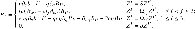 $$ \begin{align*} B_I=\left\{ \begin{array}{ll} \varepsilon\partial_sb:{I'}+q\partial_qB_{I'}, & Z^I=SZ^{I'}; \\ (\omega_i\partial_{\omega_j}-\omega_j\partial_{\omega_i})B_{I'}, & Z^I=\Omega_{ij}Z^{I'},\ 1\leq i<j\leq 3;\\ \varepsilon\omega_i\partial_sb:{I'}-q\omega_i\partial_qB_{I'}+\partial_{\omega_i}B_{I'}-2\omega_iB_{I'}, & Z^I=\Omega_{0i}Z^{I'},\ 1\leq i\leq 3;\\ 0, & Z^I=\partial Z^{I'}. \end{array}\right. \end{align*} $$
We also have $B_0=2\widehat { A }(\exp (\frac {1}{2}G(\omega )\widehat { A }s)-1)$
. Since
$B_0=2\widehat { A }(\exp (\frac {1}{2}G(\omega )\widehat { A }s)-1)$
. Since $\exp (\frac {1}{2}G(\omega )\widehat { A }s)-1$
has essentially the same form as
$\exp (\frac {1}{2}G(\omega )\widehat { A }s)-1$
has essentially the same form as $\widehat { \mu }+2$
, by following the proof of (3.18), we obtain for all
$\widehat { \mu }+2$
, by following the proof of (3.18), we obtain for all $a,b,c\geq 0$
and all
$a,b,c\geq 0$
and all $(s,q,\omega )\in [0,\infty )\times \mathbb {R}\times \mathbb {S}^2$
,
$(s,q,\omega )\in [0,\infty )\times \mathbb {R}\times \mathbb {S}^2$
,
 $$ \begin{align*} \partial_q^a\partial_s^b\partial_\omega^c (\exp(\frac{1}{2}G(\omega)\widehat{ A }s)-1)=O_{a,b,c}(\langle q \rangle^{-\max\{1,b\}-a+C_{a,b,c}\varepsilon}e^{C_{a,b,c}s}). \end{align*} $$
It follows from Leibniz’s rule that
 $$ \begin{align*} \partial_q^a\partial_s^b\partial_\omega^cB_0&=O_{a,b,c}(\langle q \rangle^{-\max\{1,b\}-1-a+C_{a,b,c}\varepsilon}e^{C_{a,b,c}s}). \end{align*} $$
Now, (3.29) follows by induction on $|I|$
. We again omit the details of the proof.
$|I|$
. We again omit the details of the proof.
3.5.1 Proof of (3.31)
By the definition of $\widehat { u }$
, in
$\widehat { u }$
, in $\Omega $
we have
$\Omega $
we have
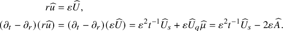 $$ \begin{align*} r\widehat{ u }&=\varepsilon\widehat{ U },\\ (\partial_t-\partial_r)(r\widehat{ u })&=(\partial_t-\partial_r)(\varepsilon\widehat{ U })=\varepsilon^2t^{-1}\widehat{ U }_s+\varepsilon\widehat{ U }_q\widehat{ \mu }=\varepsilon^2t^{-1}\widehat{ U }_s-2\varepsilon\widehat{ A }. \end{align*} $$
Here, $\widehat { U },\widehat { U }_s,\widehat { A }$
are functions of
$\widehat { U },\widehat { U }_s,\widehat { A }$
are functions of $(t,x)$
via the map
$(t,x)$
via the map $(t,x)\mapsto (\varepsilon \ln t-\delta ,\widehat { q }(t,x),x/|x|)$
. By (3.23) at the end of Section 3.4, we have
$(t,x)\mapsto (\varepsilon \ln t-\delta ,\widehat { q }(t,x),x/|x|)$
. By (3.23) at the end of Section 3.4, we have $\varepsilon \widehat { U }_s\in S^{0,0}$
. Thus, we have
$\varepsilon \widehat { U }_s\in S^{0,0}$
. Thus, we have
 $$ \begin{align*} (\partial_t-\partial_r)(r\widehat{ u })&=-2\varepsilon\widehat{ A }+\varepsilon S^{-1,0}. \end{align*} $$
It remains to show that
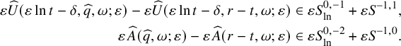 $$ \begin{align}\begin{aligned} \varepsilon \widehat{ U }(\varepsilon\ln t-\delta,\widehat{ q },\omega;\varepsilon)-\varepsilon \widehat{ U }(\varepsilon\ln t-\delta,r-t,\omega;\varepsilon)&\in \varepsilon S^{0,-1}_{\ln}+\varepsilon S^{-1,1},\\\varepsilon \widehat{ A }(\widehat{ q },\omega;\varepsilon)-\varepsilon \widehat{ A }(r-t,\omega;\varepsilon)&\in \varepsilon S^{0,-2}_{\ln}+\varepsilon S^{-1,0}. \end{aligned}\end{align} $$
We first prove a lemma for $\widehat { q }$
. This lemma both relies on and improves [Reference Yu75, Lemma 7.7].
$\widehat { q }$
. This lemma both relies on and improves [Reference Yu75, Lemma 7.7].
Lemma 3.4. We have $\widehat { q }-r+t\in S^{0,0}_{\ln }$
. That is, for each I, we have
$\widehat { q }-r+t\in S^{0,0}_{\ln }$
. That is, for each I, we have $Z^I(\widehat { q }-r+t)=O((1+\ln \langle r-t \rangle )t^{C\varepsilon })$
in
$Z^I(\widehat { q }-r+t)=O((1+\ln \langle r-t \rangle )t^{C\varepsilon })$
in $\Omega $
.
$\Omega $
.
Proof. For $r-t\geq R$
, we have
$r-t\geq R$
, we have $q=r-t$
. It remains to prove
$q=r-t$
. It remains to prove $Z^I(\widehat { q }-r+t)=O((1+\ln \langle r-t \rangle )t^{C\varepsilon })$
for each I in
$Z^I(\widehat { q }-r+t)=O((1+\ln \langle r-t \rangle )t^{C\varepsilon })$
for each I in $\Omega \cap \{r-t<2R\}$
. Before we start the proof, we recall from [Reference Yu75, Lemma 7.4] that
$\Omega \cap \{r-t<2R\}$
. Before we start the proof, we recall from [Reference Yu75, Lemma 7.4] that $t^{-C\varepsilon }\lesssim \langle \widehat { q } \rangle /\langle r-t \rangle \lesssim t^{C\varepsilon }$
in
$t^{-C\varepsilon }\lesssim \langle \widehat { q } \rangle /\langle r-t \rangle \lesssim t^{C\varepsilon }$
in $\Omega $
. Thus, every power of
$\Omega $
. Thus, every power of $\langle \widehat { q } \rangle $
can be controlled by
$\langle \widehat { q } \rangle $
can be controlled by $\langle r-t \rangle t^{C\varepsilon }$
and vice versa.
$\langle r-t \rangle t^{C\varepsilon }$
and vice versa.
We first apply Lemma 2.4 to compute $(\partial _t-\partial _r)Z^I(\widehat { q }-r+t)$
for each multiindex I. For each integer
$(\partial _t-\partial _r)Z^I(\widehat { q }-r+t)$
for each multiindex I. For each integer $N\geq 0$
, in
$N\geq 0$
, in $\Omega $
we have
$\Omega $
we have
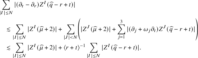 $$ \begin{align}\begin{aligned} &\sum_{|I|\leq N}|(\partial_t-\partial_r)Z^I(\widehat{ q }-r+t)|\\&\quad\lesssim \sum_{|I|\leq N}|Z^I(\widehat{ \mu }+2)|+\sum_{|J|<N}\left( |Z^J(\widehat{ \mu }+2)|+\sum_{j=1}^3|(\partial_j+\omega_j\partial_t)Z^J(\widehat{ q }-r+t)| \right)\\&\quad\lesssim \sum_{|I|\leq N}|Z^I(\widehat{ \mu }+2)|+\langle r+t \rangle^{-1}\sum_{|I|\leq N}|Z^I(\widehat{ q }-r+t)|. \end{aligned}\end{align} $$
Here, we recall that $\widehat { \mu }=\widehat { q }_t-\widehat { q }_r$
. In the last estimate, we apply Lemma 2.1 to get the factor
$\widehat { \mu }=\widehat { q }_t-\widehat { q }_r$
. In the last estimate, we apply Lemma 2.1 to get the factor $\langle r+t \rangle ^{-1}$
. Meanwhile, we recall that
$\langle r+t \rangle ^{-1}$
. Meanwhile, we recall that $\widehat { \mu }+2\in S^{0,-1}$
. In fact, the results in (3.23) hold because it is already known that
$\widehat { \mu }+2\in S^{0,-1}$
. In fact, the results in (3.23) hold because it is already known that $\widehat { q }\in S^{0,1}$
from [Reference Yu75, Lemma 7.7]. Thus, we have
$\widehat { q }\in S^{0,1}$
from [Reference Yu75, Lemma 7.7]. Thus, we have $\sum _{|I|\leq N}|Z^I(\widehat { \mu }+2)|\lesssim \langle r-t \rangle ^{-1}t^{C\varepsilon }$
in
$\sum _{|I|\leq N}|Z^I(\widehat { \mu }+2)|\lesssim \langle r-t \rangle ^{-1}t^{C\varepsilon }$
in $\Omega $
.
$\Omega $
.
We can now use Gronwall’s inequality to finish the proof. Fix an integer $N\geq 0$
and a point
$N\geq 0$
and a point $(t_0,x_0)\in \Omega \cap \{|x_0|-t_0<2R\}$
. For each
$(t_0,x_0)\in \Omega \cap \{|x_0|-t_0<2R\}$
. For each $\tau \in [\frac {t_0+|x_0|}{2}-R,t_0]$
, we set
$\tau \in [\frac {t_0+|x_0|}{2}-R,t_0]$
, we set
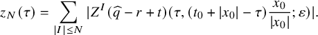 $$ \begin{align*} z_N(\tau)&=\sum_{|I|\leq N}|Z^I(\widehat{ q }-r+t)(\tau,(t_0+|x_0|-\tau)\frac{x_0}{|x_0|};\varepsilon)|. \end{align*} $$
Note that $(\tau ,(t_0+|x_0|-2\tau )\frac {x_0}{|x_0|})\in \Omega \cap \{r-t<2R\}$
for all
$(\tau ,(t_0+|x_0|-2\tau )\frac {x_0}{|x_0|})\in \Omega \cap \{r-t<2R\}$
for all $\tau \in [\frac {t_0+|x_0|}{2}-R,t_0]$
. Moreover, given a function
$\tau \in [\frac {t_0+|x_0|}{2}-R,t_0]$
. Moreover, given a function $h(t,x)$
, for
$h(t,x)$
, for $\widetilde { z }(\tau )=h(\tau ,(|x_0|+t_0-\tau )\cdot \frac {x_0}{|x_0|})$
, we have
$\widetilde { z }(\tau )=h(\tau ,(|x_0|+t_0-\tau )\cdot \frac {x_0}{|x_0|})$
, we have $\frac {d}{d\tau }\widetilde { z }=(h_t-h_r)(\tau ,(|x_0|+t_0-\tau )\cdot \frac {x_0}{|x_0|})$
. Thus, the inequality (3.34) implies that for each
$\frac {d}{d\tau }\widetilde { z }=(h_t-h_r)(\tau ,(|x_0|+t_0-\tau )\cdot \frac {x_0}{|x_0|})$
. Thus, the inequality (3.34) implies that for each $\tau _0\in [\frac {t_0+|x_0|}{2}-R,t_0]$
,
$\tau _0\in [\frac {t_0+|x_0|}{2}-R,t_0]$
,
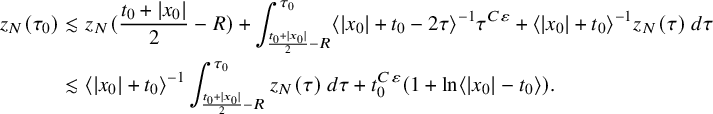 $$ \begin{align*} z_N(\tau_0)&\lesssim z_N(\frac{t_0+|x_0|}{2}-R)+\int_{\frac{t_0+|x_0|}{2}-R}^{\tau_0}\langle |x_0|+t_0-2\tau \rangle^{-1}\tau^{C\varepsilon}+\langle |x_0|+t_0 \rangle^{-1}z_N(\tau)\ d\tau\\ &\lesssim\langle |x_0|+t_0 \rangle^{-1}\int_{\frac{t_0+|x_0|}{2}-R}^{\tau_0}z_N(\tau)\ d\tau+ t_0^{C\varepsilon}(1+\ln\langle |x_0|-t_0 \rangle). \end{align*} $$
To obtain the second estimate, we notice that $(\frac {t_0+|x_0|}{2}-R,(\frac {t_0+|x_0|}{2}-R)\frac {x_0}{|x_0|})\in \{(t,x):\ |x|-t>R\}$
. Thus, we have
$(\frac {t_0+|x_0|}{2}-R,(\frac {t_0+|x_0|}{2}-R)\frac {x_0}{|x_0|})\in \{(t,x):\ |x|-t>R\}$
. Thus, we have $\widehat { q }=r-t$
near this point and thus
$\widehat { q }=r-t$
near this point and thus $z_N(\frac {t_0+|x_0|}{2}-R)=0$
. Moreover, for
$z_N(\frac {t_0+|x_0|}{2}-R)=0$
. Moreover, for $\frac {t_0+|x_0|}{2}-R\leq \tau \leq t_0$
, we have
$\frac {t_0+|x_0|}{2}-R\leq \tau \leq t_0$
, we have $\tau ^{C\varepsilon }\leq t_0^{C\varepsilon }$
and
$\tau ^{C\varepsilon }\leq t_0^{C\varepsilon }$
and $t+x_0-2\tau \leq 2R$
. It follows that
$t+x_0-2\tau \leq 2R$
. It follows that
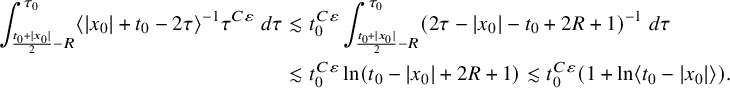 $$ \begin{align*} \int_{\frac{t_0+|x_0|}{2}-R}^{\tau_0}\langle |x_0|+t_0-2\tau \rangle^{-1}\tau^{C\varepsilon}\ d\tau&\lesssim t_0^{C\varepsilon}\int_{\frac{t_0+|x_0|}{2}-R}^{\tau_0}(2\tau-|x_0|-t_0+2R+1)^{-1}\ d\tau\\ &\lesssim t_0^{C\varepsilon}\ln(t_0-|x_0|+2R+1)\lesssim t_0^{C\varepsilon}(1+\ln\langle t_0-|x_0| \rangle). \end{align*} $$
Thus, by Gronwall’s inequality, we have
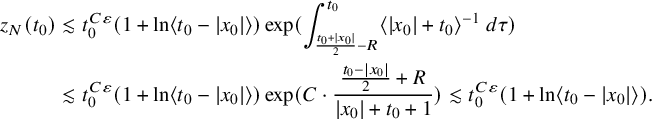 $$ \begin{align*} z_N(t_0)&\lesssim t_0^{C\varepsilon}(1+\ln\langle t_0-|x_0| \rangle)\exp(\int_{\frac{t_0+|x_0|}{2}-R}^{t_0}\langle |x_0|+t_0 \rangle^{-1}\ d\tau)\\&\lesssim t_0^{C\varepsilon}(1+\ln\langle t_0-|x_0| \rangle)\exp(C\cdot \frac{\frac{t_0-|x_0|}{2}+R}{|x_0|+t_0+1})\lesssim t_0^{C\varepsilon}(1+\ln\langle t_0-|x_0| \rangle).\\[-41pt] \end{align*} $$
Using Lemma 3.4 and the bounds for $\widehat { U },\widehat { A }$
, we now show (3.33) which implies (3.31).
$\widehat { U },\widehat { A }$
, we now show (3.33) which implies (3.31).
Lemma 3.5. Fix an integer $N\geq 0$
. Then, for
$N\geq 0$
. Then, for $\varepsilon \ll _N1$
and all
$\varepsilon \ll _N1$
and all $(t,x)\in \Omega $
, we have
$(t,x)\in \Omega $
, we have
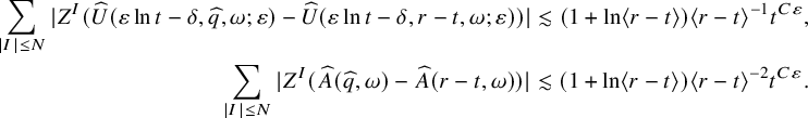 $$ \begin{align*} \sum_{|I|\leq N}|Z^I(\widehat{ U }(\varepsilon\ln t-\delta,\widehat{ q },\omega;\varepsilon)-\widehat{ U }(\varepsilon\ln t-\delta,r-t,\omega;\varepsilon))|\lesssim (1+\ln\langle r-t \rangle)\langle r-t \rangle^{-1}t^{C\varepsilon},\\ \sum_{|I|\leq N}|Z^I(\widehat{ A }(\widehat{ q },\omega)-\widehat{ A }(r-t,\omega))|\lesssim (1+\ln\langle r-t \rangle)\langle r-t \rangle^{-2}t^{C\varepsilon}. \end{align*} $$
Proof. Since $\widehat { q }=r-t$
for
$\widehat { q }=r-t$
for $r-t\geq R$
, it remains to prove this lemma in
$r-t\geq R$
, it remains to prove this lemma in $\Omega \cap \{r-t<2R\}$
. We will prove by induction on
$\Omega \cap \{r-t<2R\}$
. We will prove by induction on $|I|$
.
$|I|$
.
When $|I|=0$
, by the mean value theorem, we have (here we set
$|I|=0$
, by the mean value theorem, we have (here we set $s=\varepsilon \ln t-\delta $
and omit the parameter
$s=\varepsilon \ln t-\delta $
and omit the parameter $\varepsilon $
)
$\varepsilon $
)
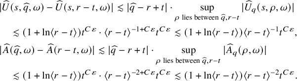 $$ \begin{align*} &|\widehat{ U }(s,\widehat{ q },\omega)-\widehat{ U }(s,r-t,\omega)|\lesssim |\widehat{ q }-r+t|\cdot \sup_{\rho\ \text{lies between }\widehat{ q },r-t}|\widehat{ U }_q(s,\rho,\omega)|\\&\quad \lesssim (1+\ln\langle r-t \rangle)t^{C\varepsilon}\cdot \langle r-t \rangle^{-1+C\varepsilon}t^{C\varepsilon}\lesssim (1+\ln\langle r-t \rangle)\langle r-t \rangle^{-1}t^{C\varepsilon},\\&|\widehat{ A }(\widehat{ q },\omega)-\widehat{ A }(r-t,\omega)|\lesssim |\widehat{ q }-r+t|\cdot \sup_{\rho\ \text{lies between }\widehat{ q },r-t}|\widehat{ A }_q(\rho,\omega)|\\&\quad \lesssim (1+\ln\langle r-t \rangle)t^{C\varepsilon}\cdot \langle r-t \rangle^{-2+C\varepsilon}t^{C\varepsilon}\lesssim (1+\ln\langle r-t \rangle)\langle r-t \rangle^{-2}t^{C\varepsilon}. \end{align*} $$
Here, we use (3.17), (3.18), and Lemma 3.4. Besides, we also use the fact that if $\rho $
lies between
$\rho $
lies between $\widehat { q }$
and
$\widehat { q }$
and $r-t$
, then
$r-t$
, then $\langle r-t \rangle \lesssim \langle \rho \rangle t^{C\varepsilon }$
. In fact, since
$\langle r-t \rangle \lesssim \langle \rho \rangle t^{C\varepsilon }$
. In fact, since $\widehat { q }<2R$
and
$\widehat { q }<2R$
and $r-t<2R$
in
$r-t<2R$
in $\Omega \cap \{r-t<2R\}$
, we also have
$\Omega \cap \{r-t<2R\}$
, we also have $\rho <2R$
. And since
$\rho <2R$
. And since $t^{-C\varepsilon }\lesssim \langle \widehat { q } \rangle /\langle r-t \rangle \lesssim t^{C\varepsilon }$
, we have
$t^{-C\varepsilon }\lesssim \langle \widehat { q } \rangle /\langle r-t \rangle \lesssim t^{C\varepsilon }$
, we have
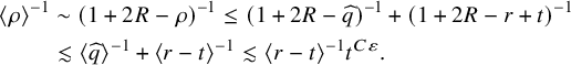 $$ \begin{align*} \langle \rho \rangle^{-1}&\sim (1+2R-\rho)^{-1}\leq (1+2R-\widehat{ q })^{-1}+(1+2R-r+t)^{-1}\\&\lesssim \langle \widehat{ q } \rangle^{-1}+\langle r-t \rangle^{-1}\lesssim \langle r-t \rangle^{-1}t^{C\varepsilon}. \end{align*} $$
We thus finish the proof when $|I|=0$
.
$|I|=0$
.
In general, we fix a multiindex I with $|I|>0$
. By the chain rule and Leibniz’s rule, we can write
$|I|>0$
. By the chain rule and Leibniz’s rule, we can write $Z^I(\widehat { U }(s,\widehat { q },\omega )-\widehat { U }(s,r-t,\omega ))$
as a linear combination (with real constant coefficients depending on I) of terms of the form
$Z^I(\widehat { U }(s,\widehat { q },\omega )-\widehat { U }(s,r-t,\omega ))$
as a linear combination (with real constant coefficients depending on I) of terms of the form
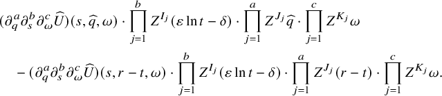 $$ \begin{align*} &(\partial_q^a\partial_s^b\partial_\omega^c \widehat{ U })(s,\widehat{ q },\omega)\cdot \prod_{j=1}^b Z^{I_j}(\varepsilon\ln t-\delta)\cdot\prod_{j=1}^a Z^{J_j}\widehat{ q }\cdot\prod_{j=1}^cZ^{K_j}\omega \\&\quad-(\partial_q^a\partial_s^b\partial_\omega^c \widehat{ U })(s,r-t,\omega)\cdot \prod_{j=1}^b Z^{I_j}(\varepsilon\ln t-\delta)\cdot\prod_{j=1}^a Z^{J_j}(r-t)\cdot\prod_{j=1}^cZ^{K_j}\omega. \end{align*} $$
Here, $a+b+c>0$
, the sum of all the multiindices is
$a+b+c>0$
, the sum of all the multiindices is $|I|$
, and each of these multiindices is nonzero. This term equals
$|I|$
, and each of these multiindices is nonzero. This term equals
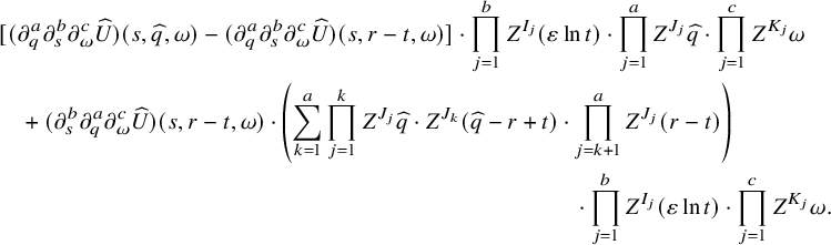 $$ \begin{align*} &[(\partial_q^a\partial_s^b\partial_\omega^c \widehat{ U })(s,\widehat{ q },\omega)-(\partial_q^a\partial_s^b\partial_\omega^c \widehat{ U })(s,r-t,\omega)]\cdot\prod_{j=1}^bZ^{I_j}(\varepsilon\ln t)\cdot\prod_{j=1}^a Z^{J_j}\widehat{ q }\cdot\prod_{j=1}^cZ^{K_j}\omega\\&\quad +(\partial_s^b\partial_q^a\partial_\omega^c \widehat{ U })(s,r-t,\omega)\cdot \left( \sum_{k=1}^a\prod_{j=1}^k Z^{J_j}\widehat{ q }\cdot Z^{J_k}(\widehat{ q }-r+t)\cdot \prod_{j=k+1}^a Z^{J_j}(r-t) \right)\\&\hspace{25em}\cdot\prod_{j=1}^bZ^{I_j}(\varepsilon\ln t)\cdot\prod_{j=1}^cZ^{K_j}\omega. \end{align*} $$
If $a=0$
, then the second row vanishes. We claim that this term is
$a=0$
, then the second row vanishes. We claim that this term is $O((1+\ln \langle r-t \rangle )\langle r-t \rangle ^{-1}t^{C\varepsilon })$
. In fact, by (3.18), we follow a similar proof in the case
$O((1+\ln \langle r-t \rangle )\langle r-t \rangle ^{-1}t^{C\varepsilon })$
. In fact, by (3.18), we follow a similar proof in the case $|I|=0$
to show that
$|I|=0$
to show that
 $$ \begin{align*} (\partial_q^a\partial_s^b\partial_\omega^c \widehat{ U })(s,\widehat{ q },\omega)-(\partial_q^a\partial_s^b\partial_\omega^c \widehat{ U })(s,r-t,\omega)=O((1+\ln\langle r-t \rangle)\langle r-t \rangle^{-1-a}t^{C\varepsilon}). \end{align*} $$
Moreover, by (3.18) and (3.19), we have $(\partial _q^a\partial _s^b\partial _\omega ^c \widehat { U })(s,r-t,\omega )=O(\langle r-t \rangle ^{-a}t^{C\varepsilon })$
in
$(\partial _q^a\partial _s^b\partial _\omega ^c \widehat { U })(s,r-t,\omega )=O(\langle r-t \rangle ^{-a}t^{C\varepsilon })$
in $\Omega \cap \{r-t<2R\}$
. We also have
$\Omega \cap \{r-t<2R\}$
. We also have $Z^J\omega =O(1)$
,
$Z^J\omega =O(1)$
, $Z^J(\widehat { q },r-t)=O(\langle r-t \rangle t^{C\varepsilon })$
, and
$Z^J(\widehat { q },r-t)=O(\langle r-t \rangle t^{C\varepsilon })$
, and $Z^J(\widehat { q }-r+t)=O((1+\ln \langle r-t \rangle )t^{C\varepsilon })$
. Combine all these estimates and we obtain the estimates for
$Z^J(\widehat { q }-r+t)=O((1+\ln \langle r-t \rangle )t^{C\varepsilon })$
. Combine all these estimates and we obtain the estimates for $\widehat { U }$
in the lemma. The estimates for
$\widehat { U }$
in the lemma. The estimates for $\widehat { A }$
can be proved similarly.
$\widehat { A }$
can be proved similarly.
3.5.2 Proof of (3.32)
We induct on $|I|$
. The case when
$|I|$
. The case when $|I|=0$
has been proved; see (3.31). Now, fix a multiindex I with
$|I|=0$
has been proved; see (3.31). Now, fix a multiindex I with $|I|>0$
and write
$|I|>0$
and write $Z^I=ZZ^{I'}$
. We have
$Z^I=ZZ^{I'}$
. We have
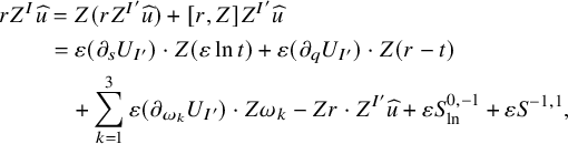 $$ \begin{align}\begin{aligned} rZ^I\widehat{ u }&= Z(rZ^{I'}\widehat{ u })+[r,Z]Z^{I'}\widehat{ u }\\ &=\varepsilon (\partial_sU_{I'})\cdot Z(\varepsilon\ln t)+\varepsilon (\partial_qU_{I'})\cdot Z(r-t)\\ &\quad +\sum_{k=1}^3\varepsilon (\partial_{\omega_k}U_{I'})\cdot Z\omega_k-Zr\cdot Z^{I'}\widehat{ u }+\varepsilon S^{0,-1}_{\ln}+\varepsilon S^{-1,1}, \end{aligned}\end{align} $$
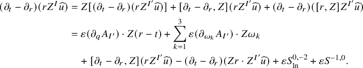 $$ \begin{align}\begin{aligned} (\partial_t-\partial_r)(rZ^I\widehat{ u })&=Z[(\partial_t-\partial_r)(rZ^{I'}\widehat{ u })]+[\partial_t-\partial_r,Z](rZ^{I'}\widehat{ u })+(\partial_t-\partial_r)([r,Z]Z^{I'}\widehat{ u })\\ &=\varepsilon (\partial_qA_{I'})\cdot Z(r-t)+\sum_{k=1}^3\varepsilon (\partial_{\omega_k}A_{I'})\cdot Z\omega_k\\ &\quad+[\partial_t-\partial_r,Z](rZ^{I'}\widehat{ u })-(\partial_t-\partial_r)(Zr\cdot Z^{I'}\widehat{ u })+\varepsilon S^{0,-2}_{\ln}+\varepsilon S^{-1,0}. \end{aligned}\end{align} $$
On the right sides, every function of $(s,q,\omega )$
is evaluated at
$(s,q,\omega )$
is evaluated at $(s,q,\omega )=(\varepsilon \ln t-\delta ,r-t,\omega )$
. For example,
$(s,q,\omega )=(\varepsilon \ln t-\delta ,r-t,\omega )$
. For example, $\partial _sU_{I'}=(\partial _sU_{I'})(\varepsilon \ln t-\delta ,r-t,\omega ;\varepsilon )$
; similarly for
$\partial _sU_{I'}=(\partial _sU_{I'})(\varepsilon \ln t-\delta ,r-t,\omega ;\varepsilon )$
; similarly for $U_{I'},A_{I'},\partial _q(U_{I'},A_{I'}),\partial _\omega (U_{I'}, A_{I'})$
. We apply the induction hypotheses and the chain rule to compute
$U_{I'},A_{I'},\partial _q(U_{I'},A_{I'}),\partial _\omega (U_{I'}, A_{I'})$
. We apply the induction hypotheses and the chain rule to compute $Z(rZ^{I'}\widehat { u })$
and
$Z(rZ^{I'}\widehat { u })$
and $Z((\partial _t-\partial _r)(rZ^{I'}\widehat { u }))$
. Now we can prove (3.32).
$Z((\partial _t-\partial _r)(rZ^{I'}\widehat { u }))$
. Now we can prove (3.32).
Lemma 3.6. Fix a multiindex I with $|I|>0$
and
$|I|>0$
and $Z^I=ZZ^{I'}$
. Assuming that (3.32) holds with I replaced by
$Z^I=ZZ^{I'}$
. Assuming that (3.32) holds with I replaced by $I'$
, we have (3.32) for I. Here, the functions
$I'$
, we have (3.32) for I. Here, the functions $U_I$
and
$U_I$
and $A_I$
are defined in the statement of Proposition 3.3.
$A_I$
are defined in the statement of Proposition 3.3.
Proof. In this proof, every function of $(s,q,\omega )$
(such as
$(s,q,\omega )$
(such as $U_{I'}$
and
$U_{I'}$
and $A_{I'}$
) is evaluated at
$A_{I'}$
) is evaluated at $(s,q,\omega )=(\varepsilon \ln t-\delta ,r-t,\omega )$
.
$(s,q,\omega )=(\varepsilon \ln t-\delta ,r-t,\omega )$
.
Since the $U_I$
’s and
$U_I$
’s and $A_I$
’s are defined inductively by (3.25) and (3.26), we can prove (3.27) and (3.28) without proving (3.24). Thus, for each multiindex I, we have
$A_I$
’s are defined inductively by (3.25) and (3.26), we can prove (3.27) and (3.28) without proving (3.24). Thus, for each multiindex I, we have
 $$ \begin{align}\begin{aligned} U_I,\varepsilon \partial_sU_I,\partial_\omega U_I\in S^{0,0};\quad \partial_qU_I,\partial_\omega A_I\in S^{0,-1};\quad \partial_qA_I\in S^{0,-2}. \end{aligned}\end{align} $$
Here, we apply Lemma 2.7 (with $\rho =r-t$
), (3.27), and (3.28).
$\rho =r-t$
), (3.27), and (3.28).
(a) Suppose that $Z^I=\partial Z^{I'}$
. We have
$Z^I=\partial Z^{I'}$
. We have $\partial (\varepsilon \ln t),\partial \omega \in \varepsilon S^{-1,0}$
and
$\partial (\varepsilon \ln t),\partial \omega \in \varepsilon S^{-1,0}$
and $\partial (r-t)\in S^{0,0}$
. By (3.37) and Lemma 2.6, we have
$\partial (r-t)\in S^{0,0}$
. By (3.37) and Lemma 2.6, we have
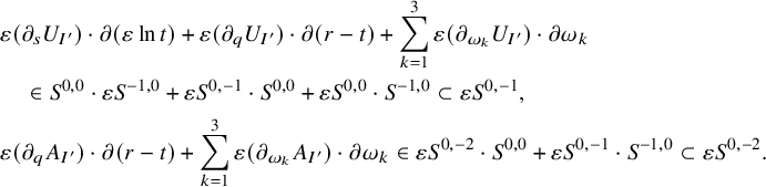 $$ \begin{align*} & \varepsilon (\partial_sU_{I'})\cdot \partial(\varepsilon\ln t)+\varepsilon (\partial_qU_{I'}) \cdot \partial(r-t)+\sum_{k=1}^3\varepsilon (\partial_{\omega_k}U_{I'}) \cdot \partial\omega_k\\&\quad \in S^{0,0}\cdot\varepsilon S^{-1,0}+\varepsilon S^{0,-1}\cdot S^{0,0}+\varepsilon S^{0,0}\cdot S^{-1,0}\subset \varepsilon S^{0,-1},\\& \varepsilon (\partial_qA_{I'}) \cdot \partial(r-t)+\sum_{k=1}^3\varepsilon (\partial_{\omega_k}A_{I'}) \cdot \partial\omega_k\in \varepsilon S^{0,-2}\cdot S^{0,0}+\varepsilon S^{0,-1}\cdot S^{-1,0}\subset \varepsilon S^{0,-2}. \end{align*} $$
Moreover, we have $[\partial _t-\partial _r,\partial _i]=r^{-1}(\partial _i-\omega _i\partial _r)=S^{-1,0}\cdot \partial $
(by
$[\partial _t-\partial _r,\partial _i]=r^{-1}(\partial _i-\omega _i\partial _r)=S^{-1,0}\cdot \partial $
(by $S^{-1,0}\cdot \partial $
we mean
$S^{-1,0}\cdot \partial $
we mean $f^\alpha (t,x) \partial _\alpha $
where
$f^\alpha (t,x) \partial _\alpha $
where $f^\alpha \in S^{0,0}$
),
$f^\alpha \in S^{0,0}$
), $\partial _ir=\omega _i\in S^{0,0}$
and
$\partial _ir=\omega _i\in S^{0,0}$
and $[\partial _t-\partial _r,\partial _t]=\partial _tr=0$
. Since
$[\partial _t-\partial _r,\partial _t]=\partial _tr=0$
. Since $\widehat { u }\in \varepsilon S^{-1,0}$
, by Lemma 2.6, we have
$\widehat { u }\in \varepsilon S^{-1,0}$
, by Lemma 2.6, we have
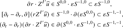 $$ \begin{align*} \partial r\cdot Z^{I'}\widehat{ u }&\in S^{0,0}\cdot \varepsilon S^{-1,0}\subset \varepsilon S^{-1,0},\\ [\partial_t-\partial_r,\partial](rZ^{I'}\widehat{ u })&\in S^{-1,0}\cdot \partial(\varepsilon S^{0,0})\subset \varepsilon S^{-1,-1},\\ (\partial_t-\partial_r)(\partial r\cdot Z^{I'}\widehat{ u })&\in \partial (S^{0,0}\cdot \varepsilon S^{-1,0})\subset \varepsilon S^{-1,-1}. \end{align*} $$
In summary, by (3.35) and (3.36), we have $ r\partial Z^{I'}\widehat { u }\in \varepsilon S^{0,-1}_{\ln }+\varepsilon S^{-1,1}$
and
$ r\partial Z^{I'}\widehat { u }\in \varepsilon S^{0,-1}_{\ln }+\varepsilon S^{-1,1}$
and $(\partial _t-\partial _r)(r\partial Z^{I'}\widehat { u })\in \varepsilon S^{0,-2}_{\ln }+\varepsilon S^{-1,0}$
, i.e.
$(\partial _t-\partial _r)(r\partial Z^{I'}\widehat { u })\in \varepsilon S^{0,-2}_{\ln }+\varepsilon S^{-1,0}$
, i.e. $U_I\equiv A_I\equiv 0$
.
$U_I\equiv A_I\equiv 0$
.
(b) Suppose that $Z^I=SZ^{I'}$
. In this case, we have
$Z^I=SZ^{I'}$
. In this case, we have $S(\varepsilon \ln t)=\varepsilon $
,
$S(\varepsilon \ln t)=\varepsilon $
, $S(r-t)=r-t$
,
$S(r-t)=r-t$
, $S\omega =0$
,
$S\omega =0$
, $[\partial _t-\partial _r,S]=\partial _t-\partial _r$
, and
$[\partial _t-\partial _r,S]=\partial _t-\partial _r$
, and $Sr=r$
. By (3.35) and (3.36), we have
$Sr=r$
. By (3.35) and (3.36), we have
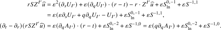 $$ \begin{align*} rSZ^{I'}\widehat{ u }&=\varepsilon^2 (\partial_sU_{I'}) +\varepsilon (\partial_qU_{I'}) \cdot (r-t) -r\cdot Z^{I'}\widehat{ u }+\varepsilon S^{0,-1}_{\ln}+\varepsilon S^{-1,1}\\ &=\varepsilon (\varepsilon \partial_sU_{I'}+q\partial_qU_{I'}-U_{I'}) +\varepsilon S^{0,-1}_{\ln}+\varepsilon S^{-1,1},\\ (\partial_t-\partial_r)(rSZ^{I'}\widehat{ u }) &=\varepsilon (\partial_qA_{I'}) \cdot (r-t)+\varepsilon S^{0,-2}_{\ln}+\varepsilon S^{-1,0}=\varepsilon(q\partial_qA_{I'})+\varepsilon S^{0,-2}_{\ln}+\varepsilon S^{-1,0}. \end{align*} $$
That is, $U_I=\varepsilon \partial _sU_{I'}+q\partial _qU_{I'}-U_{I'}$
and
$U_I=\varepsilon \partial _sU_{I'}+q\partial _qU_{I'}-U_{I'}$
and $A_I=q\partial _qA_{I'}$
. In these estimates, we apply the induction hypotheses to compute
$A_I=q\partial _qA_{I'}$
. In these estimates, we apply the induction hypotheses to compute $rZ^{I'}\widehat { u }$
. We also notice that
$rZ^{I'}\widehat { u }$
. We also notice that $[S,r(\partial _t-\partial _r)]=0$
.
$[S,r(\partial _t-\partial _r)]=0$
.
(c) Suppose that $Z^I=\Omega _{ij}Z^{I'}$
. In this case, we have
$Z^I=\Omega _{ij}Z^{I'}$
. In this case, we have $\Omega _{ij}(\varepsilon \ln t)=\Omega _{ij}(r-t)=\Omega _{ij}r=0$
,
$\Omega _{ij}(\varepsilon \ln t)=\Omega _{ij}(r-t)=\Omega _{ij}r=0$
, $\Omega _{ij}\omega _k=\omega _i\delta _{jk}-\omega _j\delta _{ik}$
, and
$\Omega _{ij}\omega _k=\omega _i\delta _{jk}-\omega _j\delta _{ik}$
, and $[\partial _t-\partial _r,\Omega _{ij}]=0$
. By (3.35) and (3.36), we have
$[\partial _t-\partial _r,\Omega _{ij}]=0$
. By (3.35) and (3.36), we have
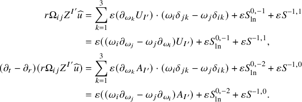 $$ \begin{align*} r\Omega_{ij}Z^{I'}\widehat{ u }&=\sum_{k=1}^3\varepsilon (\partial_{\omega_k}U_{I'}) \cdot (\omega_{i}\delta_{jk}-\omega_j\delta_{ik})+\varepsilon S^{0,-1}_{\ln}+\varepsilon S^{-1,1}\\ &=\varepsilon ((\omega_i\partial_{\omega_j}-\omega_j\partial_{\omega_i})U_{I'}) +\varepsilon S^{0,-1}_{\ln}+\varepsilon S^{-1,1},\\ (\partial_t-\partial_r)(r\Omega_{ij}Z^{I'}\widehat{ u })&=\sum_{k=1}^3\varepsilon (\partial_{\omega_k}A_{I'}) \cdot (\omega_i\delta_{jk}-\omega_j\delta_{ik})+\varepsilon S^{0,-2}_{\ln}+\varepsilon S^{-1,0}\\ &=\varepsilon ((\omega_i\partial_{\omega_j}-\omega_j\partial_{\omega_i})A_{I'}) +\varepsilon S^{0,-2}_{\ln}+\varepsilon S^{-1,0}. \end{align*} $$
That is, $U_I=(\omega _i\partial _{\omega _j}-\omega _j\partial _{\omega _i})U_{I'}$
and
$U_I=(\omega _i\partial _{\omega _j}-\omega _j\partial _{\omega _i})U_{I'}$
and $A_I=(\omega _i\partial _{\omega _j}-\omega _j\partial _{\omega _i})A_{I'}$
.
$A_I=(\omega _i\partial _{\omega _j}-\omega _j\partial _{\omega _i})A_{I'}$
.
(d) Suppose that $Z^I=\Omega _{0i}Z^{I'}$
. In this case, we have
$Z^I=\Omega _{0i}Z^{I'}$
. In this case, we have $\Omega _{0i}(\varepsilon \ln t)=\varepsilon \omega _i(1+\frac {r-t}{t}) $
,
$\Omega _{0i}(\varepsilon \ln t)=\varepsilon \omega _i(1+\frac {r-t}{t}) $
, $\Omega _{0i}(r-t)=-(r-t)\omega _i$
,
$\Omega _{0i}(r-t)=-(r-t)\omega _i$
, $\Omega _{0i}\omega _k=(1-\frac {r-t}{r})(\delta _{ik}-\omega _i\omega _k)$
,
$\Omega _{0i}\omega _k=(1-\frac {r-t}{r})(\delta _{ik}-\omega _i\omega _k)$
, $[\partial _t-\partial _r,\Omega _{0i}]=-\omega _i(\partial _t-\partial _r)-\frac {r+t}{r^2}\sum _{j=1}^3\omega _j\Omega _{ij}$
, and
$[\partial _t-\partial _r,\Omega _{0i}]=-\omega _i(\partial _t-\partial _r)-\frac {r+t}{r^2}\sum _{j=1}^3\omega _j\Omega _{ij}$
, and $\Omega _{0i}r=t\omega _i=(1-\frac {r-t}{r})r\omega _i$
. By (3.35) and (3.36), we have
$\Omega _{0i}r=t\omega _i=(1-\frac {r-t}{r})r\omega _i$
. By (3.35) and (3.36), we have
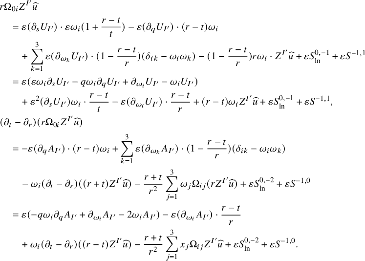 $$ \begin{align*} &r\Omega_{0i}Z^{I'}\widehat{ u }\\&\quad =\varepsilon (\partial_sU_{I'}) \cdot \varepsilon\omega_i(1+\frac{r-t}{t})-\varepsilon (\partial_qU_{I'}) \cdot (r-t)\omega_i\\&\qquad +\sum_{k=1}^3\varepsilon (\partial_{\omega_k}U_{I'}) \cdot (1-\frac{r-t}{r})(\delta_{ik}-\omega_i\omega_k)-(1-\frac{r-t}{r})r\omega_i\cdot Z^{I'}\widehat{ u }+\varepsilon S^{0,-1}_{\ln}+\varepsilon S^{-1,1}\\&\quad =\varepsilon(\varepsilon\omega_i\partial_sU_{I'}-q\omega_i\partial_qU_{I'}+\partial_{\omega_i}U_{I'}-\omega_iU_{I'})\\&\qquad+\varepsilon^2 (\partial_sU_{I'})\omega_i \cdot \frac{r-t}{t}-\varepsilon (\partial_{\omega_i}U_{I'}) \cdot \frac{r-t}{r}+(r-t)\omega_iZ^{I'}\widehat{ u }+\varepsilon S^{0,-1}_{\ln}+\varepsilon S^{-1,1},\\&(\partial_t-\partial_r)(r\Omega_{0i}Z^{I'}\widehat{ u })\\&\quad =-\varepsilon (\partial_qA_{I'}) \cdot (r-t)\omega_i+\sum_{k=1}^3\varepsilon (\partial_{\omega_k}A_{I'}) \cdot (1-\frac{r-t}{r})(\delta_{ik}-\omega_i\omega_k)\\&\qquad-\omega_i(\partial_t-\partial_r)((r+t)Z^{I'}\widehat{ u })-\frac{r+t}{r^2}\sum_{j=1}^3\omega_j\Omega_{ij}(rZ^{I'}\widehat{ u })+\varepsilon S^{0,-2}_{\ln}+\varepsilon S^{-1,0}\\&\quad =\varepsilon (-q\omega_i\partial_qA_{I'}+\partial_{\omega_i}A_{I'}-2\omega_iA_{I'}) -\varepsilon (\partial_{\omega_i}A_{I'}) \cdot \frac{r-t}{r}\\&\qquad+\omega_i(\partial_t-\partial_r)((r-t)Z^{I'}\widehat{ u })-\frac{r+t}{r^2}\sum_{j=1}^3x_j\Omega_{ij}Z^{I'}\widehat{ u }+\varepsilon S^{0,-2}_{\ln}+\varepsilon S^{-1,0}. \end{align*} $$
By (3.37), we have
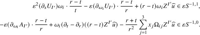 $$ \begin{align*} \varepsilon^2 (\partial_sU_{I'})\omega_i \cdot \frac{r-t}{t}-\varepsilon (\partial_{\omega_i}U_{I'}) \cdot \frac{r-t}{r}+(r-t)\omega_iZ^{I'}\widehat{ u }&\in \varepsilon S^{-1,1},\\-\varepsilon (\partial_{\omega_i}A_{I'}) \cdot \frac{r-t}{r}+\omega_i(\partial_t-\partial_r)((r-t)Z^{I'}\widehat{ u })-\frac{r+t}{r^2}\sum_{j=1}^3x_j\Omega_{ij}Z^{I'}\widehat{ u }&\in \varepsilon S^{-1,0}. \end{align*} $$
In summary, we have
 $$ \begin{align*} r\Omega_{0i}Z^{I'}\widehat{ u }&=\varepsilon(\varepsilon\omega_i\partial_sU_{I'}-q\omega_i\partial_qU_{I'}+\partial_{\omega_i}U_{I'}-\omega_iU_{I'})+\varepsilon S^{0,-1}_{\ln}+\varepsilon S^{-1,1},\\ (\partial_t-\partial_r)(r\Omega_{0i}Z^{I'}\widehat{ u }) &=\varepsilon (-q\omega_i\partial_qA_{I'}+\partial_{\omega_i}A_{I'}-2\omega_iA_{I'})+\varepsilon S^{0,-2}_{\ln}+\varepsilon S^{-1,0}. \end{align*} $$
That is, $U_I=\varepsilon \omega _i\partial _sU_{I'}-q\omega _i\partial _qU_{I'}+\partial _{\omega _i}U_{I'}-\omega _iU_{I'}$
and
$U_I=\varepsilon \omega _i\partial _sU_{I'}-q\omega _i\partial _qU_{I'}+\partial _{\omega _i}U_{I'}-\omega _iU_{I'}$
and $A_I=-q\omega _i\partial _qA_{I'}+\partial _{\omega _i}A_{I'}-2\omega _iA_{I'}$
.
$A_I=-q\omega _i\partial _qA_{I'}+\partial _{\omega _i}A_{I'}-2\omega _iA_{I'}$
.
3.6 Gauge independence
In Section 3.2, we construct the optical function $q=q(t,x;\varepsilon )$
by solving the eikonal equation (3.3). There, we consider the region
$q=q(t,x;\varepsilon )$
by solving the eikonal equation (3.3). There, we consider the region $\Omega =\Omega _{\delta ,R,\varepsilon }$
defined by (3.2) and assign the boundary condition
$\Omega =\Omega _{\delta ,R,\varepsilon }$
defined by (3.2) and assign the boundary condition $q|_{\partial \Omega }=r-t$
. Meanwhile, we will obtain different optical functions by choosing different regions
$q|_{\partial \Omega }=r-t$
. Meanwhile, we will obtain different optical functions by choosing different regions $\Omega $
and by assigning different boundary conditions. For example, for
$\Omega $
and by assigning different boundary conditions. For example, for $\overline {\delta },\kappa \in (0,1)$
, we can set
$\overline {\delta },\kappa \in (0,1)$
, we can set
 $$ \begin{align*} \overline{\Omega}_{\overline{\delta},R,\varepsilon,\kappa}=\{(t,x)\in\mathbb{R}^{1+3}:\ t>e^{\overline{\delta}/\varepsilon},\ |x|-e^{\overline{\delta}/\varepsilon}-2R>\kappa(t-e^{\overline{\delta}/\varepsilon})\} \end{align*} $$
and solve the eikonal equation (3.3) with $\Omega $
replaced by
$\Omega $
replaced by $\overline {\Omega }$
. Note that
$\overline {\Omega }$
. Note that $\Omega _{\delta ,R,\varepsilon }=\overline {\Omega }_{\delta ,R,\varepsilon ,1/2}$
. All the computations and proofs in Sections 3.2–3.5 will work, so we will again obtain functions such as
$\Omega _{\delta ,R,\varepsilon }=\overline {\Omega }_{\delta ,R,\varepsilon ,1/2}$
. All the computations and proofs in Sections 3.2–3.5 will work, so we will again obtain functions such as $\widehat { \overline {A} }$
(from (3.16)) and
$\widehat { \overline {A} }$
(from (3.16)) and $\overline {A}_I$
(from Proposition 3.3), etc. It is natural to ask how these new functions are related to the old ones. We seek to obtain a gauge independence result; see [Reference Yu75, Section 6].
$\overline {A}_I$
(from Proposition 3.3), etc. It is natural to ask how these new functions are related to the old ones. We seek to obtain a gauge independence result; see [Reference Yu75, Section 6].
For convenience, we make the following definition.
Definition 3.7. Fix $\delta ,\kappa \in (0,1)$
. Let
$\delta ,\kappa \in (0,1)$
. Let $q=q(t,x;\varepsilon )$
be a
$q=q(t,x;\varepsilon )$
be a $C^2$
optical function defined for all
$C^2$
optical function defined for all $\varepsilon \ll _{\kappa ,\delta }1$
and for all
$\varepsilon \ll _{\kappa ,\delta }1$
and for all $(t,x)\in \mathbb {R}^{1+3}$
with
$(t,x)\in \mathbb {R}^{1+3}$
with $t>e^{\delta /\varepsilon }$
and
$t>e^{\delta /\varepsilon }$
and $|x|>\kappa t$
. That is, we have
$|x|>\kappa t$
. That is, we have
 $$ \begin{align*} g^{\alpha\beta}(u)\partial_\alpha q\partial_\beta q=0,\qquad \forall t>e^{\delta/\varepsilon}, |x|>\kappa t. \end{align*} $$
Also suppose that $q|_{r-t\geq R}=r-t$
. We say that the optical function q is
$q|_{r-t\geq R}=r-t$
. We say that the optical function q is $(\delta ,\kappa )$
-admissible if it satisfies the following assumptions:
$(\delta ,\kappa )$
-admissible if it satisfies the following assumptions:
-
a) For all
$t>e^{\delta /\varepsilon }$
and
$|x|>\kappa t$
, we have
$$ \begin{align*} \sum_{|I|\leq 1}|Z^I(q_t-q_r,q_r^{-1},(q_t-q_r)^{-1})|&\lesssim t^{C\varepsilon};\\ \sum_{|I|\leq 1}\sum_{i=1,2,3}|Z^I(q_i+\omega_iq_t)|&\lesssim t^{-1+C\varepsilon}; \end{align*} $$
-
b) The map
$(s,q,\omega )=(\varepsilon \ln t-\delta ,q(t,x;\varepsilon ),x/|x|)$
induces a
$C^1$
diffeomorphism from
$\{t>e^{\delta /\varepsilon },\ |x|>\kappa t\}$
to a subset of
$[0,\infty )\times \mathbb {R}\times \mathbb {S}^2$
, so every
$C^1$
function of
$(t,x)$
induces a
$C^1$
function of
$(s,q,\omega )$
; -
c) Define
$(\mu ,U)(t,x)=(q_t-q_r,\varepsilon ^{-1}ru)(t,x)$
and consider the induced functions
$(\mu ,U)(s,q,\omega ;\varepsilon )$
. The limits in (3.5) exist; that is,
$$ \begin{align*} \left\{\begin{array}{l} \displaystyle A(q,\omega;\varepsilon):=-\frac{1}{2}\lim_{s\to\infty}(\mu U_q)(s,q,\omega;\varepsilon),\\ \displaystyle A_1(q,\omega;\varepsilon):=\lim_{s\to\infty}\exp(\frac{1}{2}G(\omega)A(q,\omega;\varepsilon)s)\mu(s,q,\omega;\varepsilon),\\ \displaystyle A_2(q,\omega;\varepsilon):=\lim_{s\to\infty}\exp(-\frac{1}{2}G(\omega)A(q,\omega;\varepsilon)s)U_q(s,q,\omega;\varepsilon). \end{array}\right. \end{align*} $$


Remark 3.7.1. For each $\kappa \in (1/2,1)$
and
$\kappa \in (1/2,1)$
and $\overline {\delta }\in [\delta ,1)$
, the optical function q constructed in Section 3.2 is
$\overline {\delta }\in [\delta ,1)$
, the optical function q constructed in Section 3.2 is $(\overline {\delta },\kappa )$
-admissible. We cannot take
$(\overline {\delta },\kappa )$
-admissible. We cannot take $\kappa =1/2$
because
$\kappa =1/2$
because $\Omega _{\delta ,R,\varepsilon }\subsetneq \{t>e^{\delta ,\varepsilon },|x|>t/2\}$
.
$\Omega _{\delta ,R,\varepsilon }\subsetneq \{t>e^{\delta ,\varepsilon },|x|>t/2\}$
.
We now state the gauge independence result. It is indeed stronger than the one in [Reference Yu75].
Proposition 3.8. Fix $\delta ,\kappa ,\overline {\delta },\overline {\kappa }\in (0,1)$
. Let
$\delta ,\kappa ,\overline {\delta },\overline {\kappa }\in (0,1)$
. Let $q,\overline {q}$
be a
$q,\overline {q}$
be a $(\delta ,\kappa )$
-admissible optical function and a
$(\delta ,\kappa )$
-admissible optical function and a $(\overline {\delta },\overline {\kappa })$
-admissible optical function, respectively. Define
$(\overline {\delta },\overline {\kappa })$
-admissible optical function, respectively. Define $\delta _0=\max \{\delta ,\overline {\delta }\}$
and
$\delta _0=\max \{\delta ,\overline {\delta }\}$
and $\kappa _0=\max \{\kappa ,\overline {\kappa }\}$
. Then, whenever
$\kappa _0=\max \{\kappa ,\overline {\kappa }\}$
. Then, whenever $\varepsilon \ll _{\delta ,\kappa ,\overline {\delta },\overline {\kappa }}1$
, we have
$\varepsilon \ll _{\delta ,\kappa ,\overline {\delta },\overline {\kappa }}1$
, we have
-
i) There exists
$Q_\infty =Q_\infty (q,\omega ;\varepsilon )\in C^1(\mathbb {R}\times \mathbb {S}^2)$
such that where
$$ \begin{align*} Q_\infty(q,\omega;\varepsilon)=\lim_{s\to\infty}\overline{q}(s,q,\omega;\varepsilon), \end{align*} $$
$\overline {q}(s,q,\omega ;\varepsilon )$
is the function induced by
$\overline {q}(t,x;\varepsilon )$
via the coordinate changes
$(s,q,\omega )=(\varepsilon \ln t-\delta ,q(t,x;\varepsilon ),x/|x|)$
. Besides, we have All the convergences are here uniform in
$$ \begin{align*} \partial_qQ_\infty=\lim_{s\to\infty}\partial_q\overline{q},\qquad \partial_{\omega_i}Q_\infty=\lim_{s\to\infty}\partial_{\omega_i}\overline{q}. \end{align*} $$
$(q,\omega )\in \mathbb {R}\times \mathbb {S}^2$
.
-
ii) One can exchange the roles of q and
$\overline {q}$
to obtain
$\overline {Q}_\infty (\overline {q},\omega ;\varepsilon )\in C^1(\mathbb {R}\times \mathbb {S}^2)$
such that Moreover, we have
$$ \begin{align*} \overline{Q}_\infty(\overline{q},\omega;\varepsilon)&=\lim_{\overline{s}\to\infty}q(\overline{s},\overline{q},\omega;\varepsilon),\\\partial_q\overline{Q}_\infty&=\lim_{\overline{s}\to\infty}\partial_{\overline{q}}q,\quad \partial_{\omega_i}\overline{Q}_\infty=\lim_{\overline{s}\to\infty}\partial_{\omega_i}q. \end{align*} $$
$$ \begin{align*} Q_\infty(\overline{Q}_\infty(\overline{q},\omega;\varepsilon),\omega;\varepsilon)&=\overline{q},\\\overline{Q}_\infty(Q_\infty(q,\omega;\varepsilon),\omega;\varepsilon)&=q. \end{align*} $$
-
iii) Let
$(A,A_1,A_2)(q,\omega ;\varepsilon )$
and
$(\overline {A},\overline {A}_1,\overline {A}_2)(\overline {q},\omega ;\varepsilon )$
be the limits defined by (3.5), respectively. Then we have
$$ \begin{align*} \overline{A}(Q_\infty(q,\omega;\varepsilon),\omega;\varepsilon)&=A(q,\omega;\varepsilon),\\ \overline{A}_1(Q_\infty(q,\omega;\varepsilon),\omega;\varepsilon)&=(A_1\cdot \partial_qQ_\infty)(q,\omega;\varepsilon)\cdot\exp(\frac{1}{2}G(\omega)A(q,\omega;\varepsilon)\cdot (\delta-\overline{\delta})). \end{align*} $$


Proof. The existence of $Q_\infty $
has been proved in [Reference Yu75, Proposition 6.1]. We recall that the key step in the proof is to write
$Q_\infty $
has been proved in [Reference Yu75, Proposition 6.1]. We recall that the key step in the proof is to write
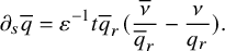 $$ \begin{align*} \partial_s\overline{q}&=\varepsilon^{-1}t\overline{q}_r(\frac{\overline{\nu}}{\overline{q}_r}-\frac{\nu}{q_r}). \end{align*} $$
Here, $\nu =q_t+q_r$
and
$\nu =q_t+q_r$
and $\overline {\nu }=\overline {q}_t+\overline {q}_r$
. Using the eikonal equation, we write
$\overline {\nu }=\overline {q}_t+\overline {q}_r$
. Using the eikonal equation, we write $\nu /q_r$
as the sum of a quantity not involving q and a remainder term. We thus obtain
$\nu /q_r$
as the sum of a quantity not involving q and a remainder term. We thus obtain $\partial _s\overline {q}=O(t^{-1+C\varepsilon })$
and show that the limit
$\partial _s\overline {q}=O(t^{-1+C\varepsilon })$
and show that the limit $Q_\infty $
exists. Following a similar proof, we can show
$Q_\infty $
exists. Following a similar proof, we can show $\partial _qQ_\infty =\lim _{s\to \infty }\partial _q\overline {q}$
and
$\partial _qQ_\infty =\lim _{s\to \infty }\partial _q\overline {q}$
and $ \partial _{\omega _i}Q_\infty =\lim _{s\to \infty }\partial _{\omega _i}\overline {q}$
. The details are skipped. This finishes the proof of part i).
$ \partial _{\omega _i}Q_\infty =\lim _{s\to \infty }\partial _{\omega _i}\overline {q}$
. The details are skipped. This finishes the proof of part i).
In part ii), we recall from the definition that both $(s,q,\omega )=(\varepsilon \ln t-\delta ,q(t,x;\varepsilon ),x/|x|)$
and
$(s,q,\omega )=(\varepsilon \ln t-\delta ,q(t,x;\varepsilon ),x/|x|)$
and $(\overline {s},\overline {q},\omega )=(\varepsilon \ln t-\overline {\delta },\overline {q}(t,x;\varepsilon ),x/|x|)$
are
$(\overline {s},\overline {q},\omega )=(\varepsilon \ln t-\overline {\delta },\overline {q}(t,x;\varepsilon ),x/|x|)$
are $C^1$
diffeomorphisms. These diffeomorphisms are defined whenever
$C^1$
diffeomorphisms. These diffeomorphisms are defined whenever $t>e^{\delta _0/\varepsilon }$
and
$t>e^{\delta _0/\varepsilon }$
and $|x|>\kappa _0t$
. We thus have two maps that are the inverses of each other:
$|x|>\kappa _0t$
. We thus have two maps that are the inverses of each other:
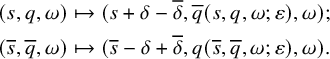 $$ \begin{align*}(s,q,\omega)\mapsto (s+\delta-\overline{\delta},\overline{q}(s,q,\omega;\varepsilon),\omega);\\(\overline{s},\overline{q},\omega)\mapsto (\overline{s}-\delta+\overline{\delta},q(\overline{s},\overline{q},\omega;\varepsilon),\omega). \end{align*} $$
It follows that for each $(s,q,\omega )$
, we have
$(s,q,\omega )$
, we have
 $$ \begin{align*} q&=q(s,\overline{q}(s+\delta-\overline{\delta},q,\omega;\varepsilon),\omega;\varepsilon). \end{align*} $$
By the continuity and the uniform convergence, we obtain
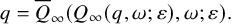 $$ \begin{align*} q=\overline{Q}_\infty(Q_\infty(q,\omega;\varepsilon),\omega;\varepsilon). \end{align*} $$
The other limit can be proved similarly.
In part iii), we have proved $\overline {A}(Q_\infty (q,\omega ;\varepsilon ),\omega ;\varepsilon )=A(q,\omega ;\varepsilon )$
in [Reference Yu75, Proposition 6.1]. To show the other limit, we recall that
$\overline {A}(Q_\infty (q,\omega ;\varepsilon ),\omega ;\varepsilon )=A(q,\omega ;\varepsilon )$
in [Reference Yu75, Proposition 6.1]. To show the other limit, we recall that
 $$ \begin{align*} \overline{A}_1(\overline{q},\omega;\varepsilon)=\lim_{\overline{s}\to\infty}\exp(\frac{1}{2}G(\omega)\overline{A}(\overline{q},\omega;\varepsilon)\overline{s})\overline{\mu}(\overline{s},\overline{q},\omega;\varepsilon). \end{align*} $$
Here, $\overline {s}=\varepsilon \ln t-\overline {\delta }=s+\delta -\overline {\delta }$
. Set
$\overline {s}=\varepsilon \ln t-\overline {\delta }=s+\delta -\overline {\delta }$
. Set $\overline {q}=Q_\infty (q,\omega ;\varepsilon )$
, and we obtain
$\overline {q}=Q_\infty (q,\omega ;\varepsilon )$
, and we obtain
 $$ \begin{align*} \overline{A}_1(Q_\infty(q,\omega;\varepsilon),\omega;\varepsilon)=\lim_{s\to\infty}\exp(\frac{1}{2}G(\omega)A(q,\omega;\varepsilon)\cdot (s+\delta-\overline{\delta}))\overline{\mu}(s+\delta-\overline{\delta},Q_\infty(q,\omega;\varepsilon),\omega;\varepsilon). \end{align*} $$
Using the $C^1$
diffeomorphisms mentioned in the proof of part ii), we identify the following three points:
$C^1$
diffeomorphisms mentioned in the proof of part ii), we identify the following three points:
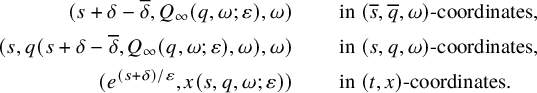 $$ \begin{align}\begin{aligned} (s+\delta-\overline{\delta},Q_\infty(q,\omega;\varepsilon),\omega)&\qquad\text{ in }(\overline{s},\overline{q},\omega)\text{-coordinates},\\(s,q(s+\delta-\overline{\delta},Q_\infty(q,\omega;\varepsilon),\omega),\omega)&\qquad\text{ in }(s,q,\omega)\text{-coordinates},\\(e^{(s+\delta)/\varepsilon},x(s,q,\omega;\varepsilon))&\qquad\text{ in }(t,x)\text{-coordinates}. \end{aligned}\end{align} $$
Here, $x(s,q,\omega ;\varepsilon )$
is chosen so that
$x(s,q,\omega ;\varepsilon )$
is chosen so that $x(s,q,\omega ;\varepsilon )=|x(s,q,\omega ;\varepsilon )|\omega $
and
$x(s,q,\omega ;\varepsilon )=|x(s,q,\omega ;\varepsilon )|\omega $
and $\overline {q}(e^{(s+\delta )/\varepsilon },x(s,q,\omega ;\varepsilon ))=Q_\infty (q,\omega )$
. Meanwhile, we have
$\overline {q}(e^{(s+\delta )/\varepsilon },x(s,q,\omega ;\varepsilon ))=Q_\infty (q,\omega )$
. Meanwhile, we have
 $$ \begin{align*} \overline{\mu}=\overline{\nu}-2\overline{q}_r=\overline{\nu}-2q_r\partial_q\overline{q}=(\mu-\nu)\partial_q\overline{q}+O(t^{-1+C\varepsilon}). \end{align*} $$
At the point specified by (3.38), we have (using $(s,q,\omega )$
-coordinates)
$(s,q,\omega )$
-coordinates)
 $$ \begin{align*} (\partial_q\overline{q})(s,\underline{q(s+\delta-\overline{\delta},Q_\infty(q,\omega;\varepsilon),\omega;\varepsilon)},\omega;\varepsilon)\to (\partial_qQ_\infty)(q,\omega;\varepsilon),\qquad s\to\infty. \end{align*} $$
This limit holds because the underlined part converges to $\overline {Q}_\infty (Q_\infty (q,\omega ;\varepsilon ),\omega ;\varepsilon )=q$
. As a result, we can skip the term
$\overline {Q}_\infty (Q_\infty (q,\omega ;\varepsilon ),\omega ;\varepsilon )=q$
. As a result, we can skip the term $-\nu \partial _q\overline {q}+O(t^{-1+C\varepsilon })$
as it will not affect the limit. In summary, we have
$-\nu \partial _q\overline {q}+O(t^{-1+C\varepsilon })$
as it will not affect the limit. In summary, we have
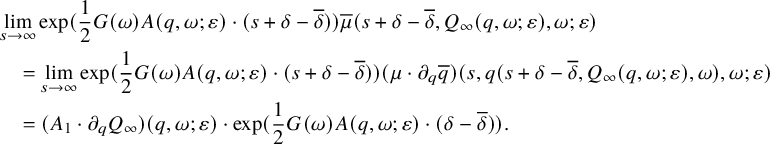 $$ \begin{align*} &\lim_{s\to\infty}\exp(\frac{1}{2}G(\omega)A(q,\omega;\varepsilon)\cdot (s+\delta-\overline{\delta}))\overline{\mu}(s+\delta-\overline{\delta},Q_\infty(q,\omega;\varepsilon),\omega;\varepsilon)\\&\quad =\lim_{s\to\infty}\exp(\frac{1}{2}G(\omega)A(q,\omega;\varepsilon)\cdot (s+\delta-\overline{\delta}))(\mu\cdot \partial_q\overline{q})(s,q(s+\delta-\overline{\delta},Q_\infty(q,\omega;\varepsilon),\omega),\omega;\varepsilon)\\&\quad =(A_1\cdot \partial_qQ_\infty)(q,\omega;\varepsilon)\cdot \exp(\frac{1}{2}G(\omega)A(q,\omega;\varepsilon)\cdot (\delta-\overline{\delta})).\\[-41pt] \end{align*} $$
We now discuss two important corollaries of this gauge independence result. First, suppose that $\delta <\overline {\delta }$
,
$\delta <\overline {\delta }$
, $\kappa <\overline {\kappa }$
, and that
$\kappa <\overline {\kappa }$
, and that $\overline {q}$
is simply a restriction of q. In this case, we have
$\overline {q}$
is simply a restriction of q. In this case, we have $Q_\infty =\overline {Q}_\infty =q$
everywhere, so part iii) of Proposition 3.8 suggests that
$Q_\infty =\overline {Q}_\infty =q$
everywhere, so part iii) of Proposition 3.8 suggests that
 $$ \begin{align*} A\equiv\overline{A},\qquad \overline{A}_1\equiv A_1\exp(\frac{\delta-\overline{\delta}}{2}G(\omega)A). \end{align*} $$
If we define $(\widetilde { \mu },\widetilde { U })$
and
$(\widetilde { \mu },\widetilde { U })$
and $(\widetilde { \overline {\mu } },\widetilde { \overline {U} })$
by (3.6) correspondingly, it is easy to check that
$(\widetilde { \overline {\mu } },\widetilde { \overline {U} })$
by (3.6) correspondingly, it is easy to check that
 $$ \begin{align*} (\widetilde{ \overline{\mu} },\widetilde{ \overline{U} })(s+\delta-\overline{\delta},q,\omega;\varepsilon)=(\widetilde{ \mu },\widetilde{ U })(s,q,\omega;\varepsilon). \end{align*} $$
Such a time translation follows from the fact that the time t corresponds to $s=\varepsilon \ln t-\delta $
in
$s=\varepsilon \ln t-\delta $
in $(s,q,\omega )$
-coordinates and
$(s,q,\omega )$
-coordinates and $\overline {s}=\varepsilon \ln t-\overline {\delta }$
in
$\overline {s}=\varepsilon \ln t-\overline {\delta }$
in $(\overline {s},\overline {q},\omega )$
-coordinates.
$(\overline {s},\overline {q},\omega )$
-coordinates.
The second corollary states that, if $\delta =\overline {\delta }$
, then the outcome
$\delta =\overline {\delta }$
, then the outcome $\widehat { A }$
defined by (3.16) should be the same.
$\widehat { A }$
defined by (3.16) should be the same.
Corollary 3.9. Fix $\delta ,\kappa ,\overline {\kappa }\in (0,1)$
. Let
$\delta ,\kappa ,\overline {\kappa }\in (0,1)$
. Let $q,\overline {q}$
be a
$q,\overline {q}$
be a $(\delta ,\kappa )$
-admissible optical function and a
$(\delta ,\kappa )$
-admissible optical function and a $(\delta ,\overline {\kappa })$
-admissible optical function, respectively. Let
$(\delta ,\overline {\kappa })$
-admissible optical function, respectively. Let $\widehat { A },\widehat { \overline {A} }$
be the functions defined by (3.16), respectively. Then we have
$\widehat { A },\widehat { \overline {A} }$
be the functions defined by (3.16), respectively. Then we have $\widehat { A }\equiv \widehat { \overline {A} }$
.
$\widehat { A }\equiv \widehat { \overline {A} }$
.
Proof. Fix $(\rho ,\omega )\in \mathbb {R}\times \mathbb {S}^2$
. We seek to prove
$(\rho ,\omega )\in \mathbb {R}\times \mathbb {S}^2$
. We seek to prove $\widehat { A }(\rho ,\omega ;\varepsilon )=\widehat { \overline {A} }(\rho ,\omega ;\varepsilon )$
, or equivalently,
$\widehat { A }(\rho ,\omega ;\varepsilon )=\widehat { \overline {A} }(\rho ,\omega ;\varepsilon )$
, or equivalently,
 $$ \begin{align*} A(\widehat{ F }(\rho,\omega;\varepsilon),\omega;\varepsilon)= \overline{A}(\widehat{ \overline{F} }(\rho,\omega;\varepsilon),\omega;\varepsilon). \end{align*} $$
The definitions of $\widehat { F },\widehat { \overline {F} }$
are given above (3.16). Since
$\widehat { F },\widehat { \overline {F} }$
are given above (3.16). Since $\overline {A}(Q_\infty (q,\omega ;\varepsilon ),\omega ;\varepsilon )=A(q,\omega ;\varepsilon )$
, it suffices to prove
$\overline {A}(Q_\infty (q,\omega ;\varepsilon ),\omega ;\varepsilon )=A(q,\omega ;\varepsilon )$
, it suffices to prove
 $$ \begin{align*} \widehat{ \overline{F} }(\rho,\omega;\varepsilon)&=Q_\infty(\widehat{ F }(\rho,\omega;\varepsilon),\omega;\varepsilon). \end{align*} $$
Set $q=\widehat { F }(\rho ,\omega ;\varepsilon )$
and
$q=\widehat { F }(\rho ,\omega ;\varepsilon )$
and $\overline {q}=\widehat { \overline {F} }(\rho ,\omega ;\varepsilon )$
. By the definitions, we have
$\overline {q}=\widehat { \overline {F} }(\rho ,\omega ;\varepsilon )$
. By the definitions, we have
 $$ \begin{align*} \rho=F(q,\omega;\varepsilon)=\overline{F}(\overline{q},\omega;\varepsilon). \end{align*} $$
We seek to prove $\overline {q}=Q_\infty (q,\omega ;\varepsilon )$
. Note that
$\overline {q}=Q_\infty (q,\omega ;\varepsilon )$
. Note that
 $$ \begin{align*} F(q,\omega;\varepsilon)&=2R-\int_{2R}^{q}\frac{2}{A_1(p,\omega;\varepsilon)}\ dp=2R-\int_{2R}^{q}\frac{2\partial_qQ_\infty(p,\omega;\varepsilon)}{\overline{A}_1(Q_\infty(p,\omega;\varepsilon),\omega;\varepsilon)}\ dp\\ &=2R-\int_{2R}^{Q_\infty(q,\omega;\varepsilon)}\frac{2}{\overline{A}_1(p,\omega;\varepsilon)}\ dp=\overline{F}(Q_\infty(q,\omega;\varepsilon),\omega;\varepsilon). \end{align*} $$
In the second identity, we use part iii) of Proposition 3.8. Since $Q_\infty (\cdot ;\omega ;\varepsilon )$
has an inverse, its derivative with respect to q cannot vanish. Moreover, since
$Q_\infty (\cdot ;\omega ;\varepsilon )$
has an inverse, its derivative with respect to q cannot vanish. Moreover, since $q,\overline {q}=r-t$
for
$q,\overline {q}=r-t$
for $r-t\geq R$
, we have
$r-t\geq R$
, we have $Q_\infty (2R,\omega ;\varepsilon )=2R$
. It follows that
$Q_\infty (2R,\omega ;\varepsilon )=2R$
. It follows that
 $$ \begin{align*} \rho=F(q,\omega;\varepsilon)=\overline{F}(Q_\infty(q,\omega;\varepsilon),\omega;\varepsilon)=\overline{F}(\overline{q},\omega;\varepsilon). \end{align*} $$
Since $\partial _q\overline {F}=2/A_1\neq 0$
, we must have
$\partial _q\overline {F}=2/A_1\neq 0$
, we must have $\overline {q}=Q_\infty (q,\omega ;\varepsilon )$
. This finishes our proof.
$\overline {q}=Q_\infty (q,\omega ;\varepsilon )$
. This finishes our proof.
4 A general result for inhomogeneous wave equations
We now consider the following general inhomogeneous wave equation:
 $$ \begin{align}\begin{aligned} \Box \phi=F(t,x)\qquad \text{in }\mathcal{O}. \end{aligned}\end{align} $$
Here, the region $\mathcal {O}\subset \mathbb {R}^{1+3}$
is defined by
$\mathcal {O}\subset \mathbb {R}^{1+3}$
is defined by
 $$ \begin{align}\begin{aligned} \mathcal{O}=\{(t,x)\in\mathbb{R}^{1+3}:\ t>0,\ |x|<t\}. \end{aligned}\end{align} $$
The main proposition in this section is a representation formula for a solution $\phi $
in
$\phi $
in $\mathcal {O}$
.
$\mathcal {O}$
.
Proposition 4.1. Suppose that $\phi \in C^2(\mathcal {O})$
is a solution to (4.1). Suppose that for some constants
$\phi \in C^2(\mathcal {O})$
is a solution to (4.1). Suppose that for some constants $M,\gamma _1,\gamma _2>0$
, we have
$M,\gamma _1,\gamma _2>0$
, we have
 $$ \begin{align*} |F(t,x)|\leq M\langle t \rangle^{-\gamma_1}\langle |x|-t \rangle^{-\gamma_2},\qquad \forall (t,x)\in\mathcal{O}. \end{align*} $$
Then, by setting $\Phi (t,x)=(-\partial _t+\partial _r)(|x|\phi )$
, for all
$\Phi (t,x)=(-\partial _t+\partial _r)(|x|\phi )$
, for all $(t,x)\in \mathcal {O}$
and
$(t,x)\in \mathcal {O}$
and $T> 2t$
, we have
$T> 2t$
, we have
 $$ \begin{align}\begin{aligned} \phi(t,x)&=\frac{1}{4\pi}\int_{\mathbb{S}^2}\Phi(T,x-(T-t)\theta)\ dS_\theta\\ &\quad+O(|x|\left\lVert\partial\phi(T)\right\rVert_{L^\infty}+M\langle t-|x| \rangle^{-\gamma_2}\cdot(\langle t \rangle^{2-\gamma_1}+\int_{t^2}^{(T-t)^2} (1+\rho)^{-\gamma_1/2}\ d\rho)). \end{aligned}\end{align} $$
The implicit constant in $O(\dots )$
is universal and does not depend on
$O(\dots )$
is universal and does not depend on $T,t,x,M,\gamma _1,\gamma _2$
.
$T,t,x,M,\gamma _1,\gamma _2$
.
Remark 4.1.1. Note that the integral can be estimated explicitly:
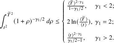 $$ \begin{align*} \int_{t^2}^{\widetilde{ T }^2}(1+\rho)^{-\gamma_1/2}\ d\rho\leq \left\{ \begin{array}{ll} \frac{\langle \widetilde{ T } \rangle^{2-\gamma_1}}{1-\gamma_1/2}, & \gamma_1<2; \\[1em] 2\ln(\frac{\langle \widetilde{ T } \rangle}{\langle t \rangle}), & \gamma_1=2;\\[1em] \frac{\langle t \rangle^{2-\gamma_1}}{\gamma_1/2-1}, & \gamma_1>2. \end{array} \right. \end{align*} $$
It suffices to prove this proposition for $M=1$
. For general
$M=1$
. For general $M>0$
, we simply replace
$M>0$
, we simply replace $(\phi ,F)$
with
$(\phi ,F)$
with $(\phi /M,F/M)$
in (4.1). In the proof, we view
$(\phi /M,F/M)$
in (4.1). In the proof, we view $\phi $
as a solution to (4.1) with initial data
$\phi $
as a solution to (4.1) with initial data $(\phi _0,\phi _1)=(\phi ,\phi _t)(T)$
at
$(\phi _0,\phi _1)=(\phi ,\phi _t)(T)$
at $t=T$
. This allows us to write
$t=T$
. This allows us to write $\phi =\phi _{\mathrm {lin}}+\phi _{\mathrm {inh}}$
. Here, we have
$\phi =\phi _{\mathrm {lin}}+\phi _{\mathrm {inh}}$
. Here, we have $\phi _{\mathrm {lin}}$
solves
$\phi _{\mathrm {lin}}$
solves $\Box \phi _{\mathrm {lin}}=0$
with data
$\Box \phi _{\mathrm {lin}}=0$
with data $(\phi _0,\phi _1)$
at
$(\phi _0,\phi _1)$
at $t=T$
, and
$t=T$
, and $\phi _{\mathrm {inh}}$
solves (4.1) with zero data at
$\phi _{\mathrm {inh}}$
solves (4.1) with zero data at $t=T$
. See Lemma 4.2. Note that
$t=T$
. See Lemma 4.2. Note that $\phi _{\mathrm {lin}}$
can be expressed explicitly in terms of
$\phi _{\mathrm {lin}}$
can be expressed explicitly in terms of $(\phi _0,\phi _1)$
and that
$(\phi _0,\phi _1)$
and that $\phi _{\mathrm {inh}}$
can be expressed explicitly in terms of F. In Lemmas 4.3 and 4.4, we estimate
$\phi _{\mathrm {inh}}$
can be expressed explicitly in terms of F. In Lemmas 4.3 and 4.4, we estimate $\phi _{\mathrm {lin}}$
and
$\phi _{\mathrm {lin}}$
and $\phi _{\mathrm {inh}}$
by applying these explicit formulas.
$\phi _{\mathrm {inh}}$
by applying these explicit formulas.
4.1 A representation formula
Lemma 4.2. Let $\phi \in C^2(\mathcal {O})$
be a solution to (4.1). Then, for all
$\phi \in C^2(\mathcal {O})$
be a solution to (4.1). Then, for all $(t,x)\in \mathcal {O}$
and
$(t,x)\in \mathcal {O}$
and $T> t$
, we have
$T> t$
, we have
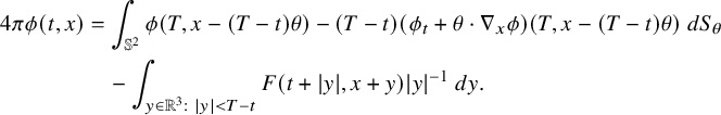 $$ \begin{align}\begin{aligned} 4\pi \phi(t,x)&=\int_{\mathbb{S}^2} \phi(T,x-(T-t)\theta)-(T-t)(\phi_t+\theta\cdot\nabla_x\phi)(T,x-(T-t)\theta)\ dS_\theta\\ &\quad -\int_{y\in\mathbb{R}^3:\ |y|<T-t}F(t+|y|,x+y) |y|^{-1}\ dy. \end{aligned}\end{align} $$
Proof. Fix $T>0$
and set
$T>0$
and set $w(t,x)=\phi (T-t,-x)$
. Note that
$w(t,x)=\phi (T-t,-x)$
. Note that $w\in C^2(\{0<t<T,\ |x|<T-t\})$
and that w solves
$w\in C^2(\{0<t<T,\ |x|<T-t\})$
and that w solves $(\Box w)(t,x)=F(T-t,-x)$
in its domain. Using formulas from, for example, [Reference Sogge67, Reference Hörmander26], we can explicitly express w in terms of
$(\Box w)(t,x)=F(T-t,-x)$
in its domain. Using formulas from, for example, [Reference Sogge67, Reference Hörmander26], we can explicitly express w in terms of $(w,w_t)|_{t=0}$
and F. Whenever
$(w,w_t)|_{t=0}$
and F. Whenever $t\in (0,T)$
and
$t\in (0,T)$
and $|x|<T-t$
, we have
$|x|<T-t$
, we have
 $$ \begin{align*} 4\pi w(t,x)&=\int_{\mathbb{S}^2}\partial_t(tw(0,x+t\theta))+tw_t(0,x+t\theta)\ dS_\theta-\int_{y\in\mathbb{R}^3:\ |y|<t}(\Box w)(t-|y|,x-y)\ \frac{dy}{|y|}. \end{align*} $$
Since $(w,w_t)|_{t=0}=(\phi (T,-x),-\phi _t(T,-x))$
, by the chain rule, we have
$(w,w_t)|_{t=0}=(\phi (T,-x),-\phi _t(T,-x))$
, by the chain rule, we have
 $$ \begin{align*} &\partial_t(tw(0,x+t\theta))+tw_t(0,x+t\theta)=w(0,x+t\theta)+t(w_t+\theta\cdot \nabla_xw)(0,x+t\theta)\\&\quad =\phi(T,-x-t\theta)-t(\phi_t+\theta\cdot \nabla_x \phi)(T,-x-t\theta). \end{align*} $$
And since $(\Box w)(t-|y|,x-y)=F(T-t+|y|,y-x)$
, we have
$(\Box w)(t-|y|,x-y)=F(T-t+|y|,y-x)$
, we have
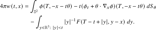 $$ \begin{align*} 4\pi w(t,x)&=\int_{\mathbb{S}^2}\phi(T,-x-t\theta)-t(\phi_t+\theta\cdot \nabla_x \phi)(T,-x-t\theta)\ dS_\theta\\ &\quad-\int_{y\in\mathbb{R}^3:\ |y|<t}|y|^{-1}F(T-t+|y|,y-x)\ dy. \end{align*} $$
Finally, by replacing $(t,x)$
with
$(t,x)$
with $(T-t,-x)$
, we obtain the formula for
$(T-t,-x)$
, we obtain the formula for $\phi $
. This is because
$\phi $
. This is because $\phi (t,x)=w(T-t,-x)$
.
$\phi (t,x)=w(T-t,-x)$
.
For each $(t,x)\in \mathcal {O}$
and
$(t,x)\in \mathcal {O}$
and $T>t$
, we rewrite (4.4) as
$T>t$
, we rewrite (4.4) as $\phi =\phi _{\mathrm {lin}}+\phi _{\mathrm {inh}}$
where
$\phi =\phi _{\mathrm {lin}}+\phi _{\mathrm {inh}}$
where
 $$ \begin{align}\phi_{\mathrm{lin}}(t,x;T)&=\frac{1}{4\pi}\int_{\mathbb{S}^2} \phi(T,x-(T-t)\theta)-(T-t)(\phi_t+\theta\cdot\nabla_x\phi)(T,x-(T-t)\theta)\ dS_\theta, \end{align} $$
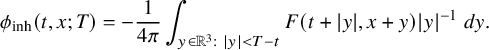 $$ \begin{align}\phi_{\mathrm{inh}}(t,x;T)&=-\frac{1}{4\pi}\int_{y\in\mathbb{R}^3:\ |y|<T-t}F(t+|y|,x+y) |y|^{-1}\ dy.\end{align} $$
When T is fixed, we note that $\phi _{\mathrm {lin}}$
is the solution to the linear wave equation
$\phi _{\mathrm {lin}}$
is the solution to the linear wave equation $\Box \phi _{\mathrm {lin}}=0$
in
$\Box \phi _{\mathrm {lin}}=0$
in $\mathcal {O}\cap \{0<t<T\}$
with data
$\mathcal {O}\cap \{0<t<T\}$
with data $(\phi _{\mathrm {lin}},\partial _t\phi _{\mathrm {lin}})|_{t=T}=(\phi (T),\phi _t(T))$
and that
$(\phi _{\mathrm {lin}},\partial _t\phi _{\mathrm {lin}})|_{t=T}=(\phi (T),\phi _t(T))$
and that $\phi _{\mathrm {inh}}$
is the solution to the inhomogeneous equation
$\phi _{\mathrm {inh}}$
is the solution to the inhomogeneous equation $\Box \phi _{\mathrm {inh}}=F$
in
$\Box \phi _{\mathrm {inh}}=F$
in $\mathcal {O}\cap \{0<t<T\}$
with zero data at
$\mathcal {O}\cap \{0<t<T\}$
with zero data at $t=T$
.
$t=T$
.
In the next two subsections, we will estimate $\phi _{\mathrm {lin}}$
and
$\phi _{\mathrm {lin}}$
and $\phi _{\mathrm {inh}}$
, respectively. Proposition 4.1 will then follow directly from Lemmas 4.3 and 4.4 below.
$\phi _{\mathrm {inh}}$
, respectively. Proposition 4.1 will then follow directly from Lemmas 4.3 and 4.4 below.
4.2 Estimates for
$\phi _{\mathrm {lin}}$

Let us start with $\phi _{\mathrm {lin}}$
defined by (4.5).
$\phi _{\mathrm {lin}}$
defined by (4.5).
Lemma 4.3. Set $\Phi (t,x)=(-\partial _t+\partial _r)(|x|\phi )$
. Then, for all
$\Phi (t,x)=(-\partial _t+\partial _r)(|x|\phi )$
. Then, for all $(t,x)\in \mathcal {O}$
with
$(t,x)\in \mathcal {O}$
with $t<T$
, we have
$t<T$
, we have
 $$ \begin{align*} \phi_{\mathrm{lin}}(t,x;T)&=\frac{1}{4\pi}\int_{\mathbb{S}^2} \Phi(T,x-(T-t)\theta)\ dS_\theta+O(|x|\left\lVert\partial\phi(T)\right\rVert_{L^\infty(\{x\in\mathbb{R}^3:\ |x|<T\})}). \end{align*} $$
The implicit constant in $O(\dots )$
is universal and does not depend on
$O(\dots )$
is universal and does not depend on $T,t,x$
.
$T,t,x$
.
Proof. For simplicity, we write $y=y(t,x,\theta ,T)=x-(T-t)\theta $
. Then, we have
$y=y(t,x,\theta ,T)=x-(T-t)\theta $
. Then, we have
 $$ \begin{align*} \Phi(T,y)&=\phi(T,y)-|y|(\phi_t-\phi_r)(T,y)=\phi(T,y)-|y|\phi_t(T,y)+\sum_{j=1}^3y_j\phi_{y_j}(T,y), \end{align*} $$
while the integrand on the right side of (4.5) is
 $$ \begin{align*} \phi(T,y)-(T-t)(\phi_t+\theta\cdot\nabla_y\phi)(T,y)=\phi(T,y)-(T-t)\phi_t(T,y)-\sum_{j=1}^3\theta_j(T-t)\phi_{y_j}(T,y). \end{align*} $$
The difference between these two formulas is $(T-t-|y|)\phi _t(T,y)+\sum _{j=1}^3(y_j+(T-t)\theta _j)\phi _{y_j}(T,y)$
. By the definition of y, we have
$(T-t-|y|)\phi _t(T,y)+\sum _{j=1}^3(y_j+(T-t)\theta _j)\phi _{y_j}(T,y)$
. By the definition of y, we have $y_j+(T-t)\theta _j=x_j$
and
$y_j+(T-t)\theta _j=x_j$
and
 $$ \begin{align*} T-t-|x|&\leq |y|=|x-(T-t)\theta|\leq |x|+T-t\Longrightarrow |T-t-|y||\leq |x|. \end{align*} $$
Here, we use $\theta \in \mathbb {S}^2$
and
$\theta \in \mathbb {S}^2$
and $T\geq t$
. This finishes the proof.
$T\geq t$
. This finishes the proof.
4.3 Estimates for
$\phi _{\mathrm {inh}}$

We now estimate $\phi _{\mathrm {inh}}$
defined by (4.6).
$\phi _{\mathrm {inh}}$
defined by (4.6).
Lemma 4.4. Suppose that $|F(t,x)|\leq \langle t \rangle ^{-\gamma _1}\langle |x|-t \rangle ^{-\gamma _2}$
in
$|F(t,x)|\leq \langle t \rangle ^{-\gamma _1}\langle |x|-t \rangle ^{-\gamma _2}$
in $\mathcal {O}$
for some constants
$\mathcal {O}$
for some constants $\gamma _1,\gamma _2>0$
. Then, for all
$\gamma _1,\gamma _2>0$
. Then, for all $t,x,\widetilde { T }$
with
$t,x,\widetilde { T }$
with $(t,x)\in \mathcal {O}$
and
$(t,x)\in \mathcal {O}$
and $\widetilde { T }>t$
(later we will set
$\widetilde { T }>t$
(later we will set $\widetilde { T }=T-t$
), we have
$\widetilde { T }=T-t$
), we have
 $$ \begin{align*} \left| \int_{y\in\mathbb{R}^3:\ |y|<\widetilde{ T }}F(t+|y|,x+y)|y|^{-1}\ dy \right| \leq 2\pi \langle t-|x| \rangle^{-\gamma_2}\cdot(\langle t \rangle^{2-\gamma_1}+\int_{t^2}^{\widetilde{ T }^2} (1+\rho)^{-\gamma_1/2}\ d\rho). \end{align*} $$
Proof. Using the bound for F, we have
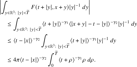 $$ \begin{align*} &\left| \int_{y\in\mathbb{R}^3:\ |y|<\widetilde{ T }}F(t+|y|,x+y)|y|^{-1}\ dy \right|\\&\quad\leq \int_{y\in\mathbb{R}^3:\ |y|<\widetilde{ T }}\langle t+|y| \rangle^{-\gamma_1}\langle |x+y|-t-|y| \rangle^{-\gamma_2}|y|^{-1}\ dy\\&\quad\leq \langle t-|x| \rangle^{-\gamma_2}\int_{y\in\mathbb{R}^3:\ |y|<\widetilde{ T }}\langle t+|y| \rangle^{-\gamma_1}|y|^{-1}\ dy\\&\quad\leq 4\pi \langle t-|x| \rangle^{-\gamma_2}\int_{0}^{\widetilde{ T }}\langle t+\rho \rangle^{-\gamma_1}\rho\ d\rho. \end{align*} $$
To get the second estimate, we recall $|x|<t$
and
$|x|<t$
and $|x+y|-|y|\leq |x|$
. Since
$|x+y|-|y|\leq |x|$
. Since $s\mapsto \langle s \rangle $
is increasing for
$s\mapsto \langle s \rangle $
is increasing for $s\geq 0$
, we have
$s\geq 0$
, we have $\langle t-|x+y|+|y| \rangle \geq \langle t-|x| \rangle $
. In the last step, we write the integral in polar coordinates.
$\langle t-|x+y|+|y| \rangle \geq \langle t-|x| \rangle $
. In the last step, we write the integral in polar coordinates.
Next, we notice that
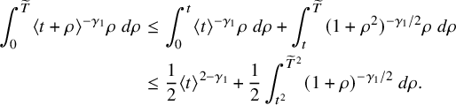 $$ \begin{align*} \int_{0}^{\widetilde{ T }}\langle t+\rho \rangle^{-\gamma_1}\rho\ d\rho&\leq \int_{0}^{t}\langle t \rangle^{-\gamma_1}\rho\ d\rho+\int_{t}^{\widetilde{ T }}(1+\rho^2)^{-\gamma_1/2}\rho\ d\rho\\ &\leq \frac{1}{2}\langle t \rangle^{2-\gamma_1}+\frac{1}{2}\int_{t^2}^{\widetilde{ T }^2}(1+\rho)^{-\gamma_1/2}\ d\rho. \end{align*} $$
This finishes the proof.
It is now obvious that Proposition 4.1 follows directly from Lemmas 4.3 and 4.4. We also note that we assume $T>2t$
in Proposition 4.1 because
$T>2t$
in Proposition 4.1 because $T-t=\widetilde { T }>t$
in Lemma 4.4.
$T-t=\widetilde { T }>t$
in Lemma 4.4.
5 Proof of Theorem 1
We now prove Theorem 1. Let u be the global solution to (1.1) in the statement of the theorem. In Section 5.1, we apply Proposition 4.1 to $\phi =Z^Iu$
for a fixed multiindex I. Because of (5.2), it remains to compute the integral
$\phi =Z^Iu$
for a fixed multiindex I. Because of (5.2), it remains to compute the integral
 $$ \begin{align*} \int_{\mathbb{S}^2}\Phi_I(T,x-(T-t)\theta;\varepsilon)\ dS_\theta, \end{align*} $$
where $\Phi _I=(-\partial _t+\partial _r)(rZ^Iu)$
. This computation is then done in Section 5.2. By settingFootnote
14
$\Phi _I=(-\partial _t+\partial _r)(rZ^Iu)$
. This computation is then done in Section 5.2. By settingFootnote
14 $T=t^3$
and
$T=t^3$
and $y=y(t,x,T,\theta )=x-(T-t)\theta $
, we have
$y=y(t,x,T,\theta )=x-(T-t)\theta $
, we have $(T,y)\in \Omega $
and
$(T,y)\in \Omega $
and $||y|-T|\lesssim T^{1/3}$
whenever
$||y|-T|\lesssim T^{1/3}$
whenever $t>(2e^{\delta /\varepsilon })^{1/3}$
,
$t>(2e^{\delta /\varepsilon })^{1/3}$
, $|x|<t$
, and
$|x|<t$
, and $\theta \in \mathbb {S}^2$
. Here, we recall that
$\theta \in \mathbb {S}^2$
. Here, we recall that $\Omega =\Omega _{\delta ,R,\varepsilon }$
was defined by (3.2). As a result, we can apply (3.14) to show
$\Omega =\Omega _{\delta ,R,\varepsilon }$
was defined by (3.2). As a result, we can apply (3.14) to show
 $$ \begin{align*} \Phi_I(T,y;\varepsilon)\approx -r(\partial_t-\partial_r)Z^I\widetilde{ u }(T,y;\varepsilon). \end{align*} $$
Moreover, by Proposition 3.3, we also have
 $$ \begin{align*} -r(\partial_t-\partial_r)Z^I\widetilde{ u }(T,y;\varepsilon)=-r(\partial_t-\partial_r)Z^I\widehat{ u }(T,y;\varepsilon)\approx -\varepsilon A_I(|y|-T,y/|y|;\varepsilon). \end{align*} $$
Finally, by Lemma 5.1, we have $|y|-T\approx -t-x\cdot \theta $
and
$|y|-T\approx -t-x\cdot \theta $
and $y/|y|\approx -\theta $
. We thus have
$y/|y|\approx -\theta $
. We thus have
 $$ \begin{align*} \int_{\mathbb{S}^2}\Phi_I(T,x-(T-t)\theta;\varepsilon)\ dS_\theta\approx -\varepsilon\int_{\mathbb{S}^2}A_I(-t-x\cdot\theta,-\theta;\varepsilon)\ dS_\theta. \end{align*} $$
Thus, we obtain the integral on the right-hand side of (1.23). We still need to estimate the error terms in these computations. The details will be given in the proof below.
5.1 Setup
Fix $(u_0,u_1)\in C_c^\infty (\mathbb {R}^3)$
. Let u be the global
$(u_0,u_1)\in C_c^\infty (\mathbb {R}^3)$
. Let u be the global $C^\infty $
solution to (1.1) with data
$C^\infty $
solution to (1.1) with data $(\varepsilon u_0,\varepsilon u_1)$
for
$(\varepsilon u_0,\varepsilon u_1)$
for $\varepsilon \ll 1$
. Now fix a multiindex I. Set
$\varepsilon \ll 1$
. Now fix a multiindex I. Set $N=|I|+2$
and choose
$N=|I|+2$
and choose $\varepsilon \ll _N1$
so that (3.1) holds for N.
$\varepsilon \ll _N1$
so that (3.1) holds for N.
In order to apply Proposition 4.1 to $Z^Iu$
, we need to estimate
$Z^Iu$
, we need to estimate $\Box Z^I u$
. In fact, since
$\Box Z^I u$
. In fact, since $g^{\alpha \beta }(u)=m^{\alpha \beta }+O(|u|)$
, it follows from (3.1) and Lemma 2.3 (with
$g^{\alpha \beta }(u)=m^{\alpha \beta }+O(|u|)$
, it follows from (3.1) and Lemma 2.3 (with $l_0=1$
) that
$l_0=1$
) that
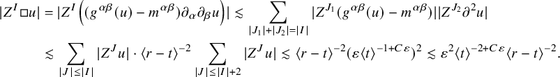 $$ \begin{align*} |Z^I\Box u|&=|Z^I\left( (g^{\alpha\beta}(u)-m^{\alpha\beta})\partial_\alpha\partial_\beta u \right)|\lesssim \sum_{|J_1|+|J_2|=|I|}|Z^{J_1}(g^{\alpha\beta}(u)-m^{\alpha\beta})||Z^{J_2}\partial^2u|\\ &\lesssim \sum_{|J|\leq |I|}|Z^Ju| \cdot\langle r-t \rangle^{-2}\sum_{|J|\leq |I|+2}|Z^Ju|\lesssim \langle r-t \rangle^{-2}(\varepsilon \langle t \rangle^{-1+C\varepsilon})^2\lesssim \varepsilon^2 \langle t \rangle^{-2+C\varepsilon}\langle r-t \rangle^{-2}. \end{align*} $$
Now we apply Proposition 4.1 to $Z^Iu$
(with
$Z^Iu$
(with $M=C\varepsilon ^2$
,
$M=C\varepsilon ^2$
, $\gamma _1=2-C\varepsilon $
and
$\gamma _1=2-C\varepsilon $
and $\gamma _2=2$
). By setting
$\gamma _2=2$
). By setting $\Phi _I(t,x;\varepsilon )=(-\partial _t+\partial _r)(rZ^Iu)(t,x;\varepsilon )$
, for all
$\Phi _I(t,x;\varepsilon )=(-\partial _t+\partial _r)(rZ^Iu)(t,x;\varepsilon )$
, for all $(t,x)$
with
$(t,x)$
with $t>0$
and
$t>0$
and $|x|<t$
, and all
$|x|<t$
, and all $T>2t$
, we have
$T>2t$
, we have
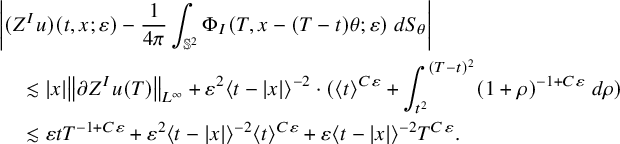 $$ \begin{align}\begin{aligned} &\left| (Z^Iu)(t,x;\varepsilon)-\frac{1}{4\pi}\int_{\mathbb{S}^2}\Phi_I(T,x-(T-t)\theta;\varepsilon)\ dS_\theta \right|\\&\quad\lesssim|x|\left\lVert\partial Z^Iu(T)\right\rVert_{L^\infty}+\varepsilon^2\langle t-|x| \rangle^{-2}\cdot(\langle t \rangle^{C\varepsilon}+\int_{t^2}^{(T-t)^2} (1+\rho)^{-1+C\varepsilon}\ d\rho)\\&\quad\lesssim \varepsilon tT^{-1+C\varepsilon}+\varepsilon^2\langle t-|x| \rangle^{-2}\langle t \rangle^{C\varepsilon}+\varepsilon\langle t-|x| \rangle^{-2}T^{C\varepsilon}. \end{aligned}\end{align} $$
If $t>2$
and if we set
$t>2$
and if we set $T=t^3>2t$
, then
$T=t^3>2t$
, then $T^{C\varepsilon }\lesssim t^{C\varepsilon }$
and
$T^{C\varepsilon }\lesssim t^{C\varepsilon }$
and $tT^{-1+C\varepsilon }\lesssim t^{-2+C\varepsilon }\lesssim \langle t-|x| \rangle ^{-2}t^{C\varepsilon }$
(since
$tT^{-1+C\varepsilon }\lesssim t^{-2+C\varepsilon }\lesssim \langle t-|x| \rangle ^{-2}t^{C\varepsilon }$
(since $0<t-|x|<t$
). That is, we have
$0<t-|x|<t$
). That is, we have
 $$ \begin{align}\begin{aligned} \left| (Z^Iu)(t,x;\varepsilon)-\frac{1}{4\pi}\int_{\mathbb{S}^2}\Phi_I(T,x-(T-t)\theta;\varepsilon)\ dS_\theta \right|\lesssim \varepsilon \langle t-|x| \rangle^{-2}t^{C\varepsilon}. \end{aligned}\end{align} $$
It remains to compute the integral of $\Phi _I$
.
$\Phi _I$
.
5.2 Computing the integral of
$\Phi _I$

We now apply the results in Section 3. Since most estimates there hold in $\Omega $
defined by (3.2), our first goal is to show that
$\Omega $
defined by (3.2), our first goal is to show that
 $$ \begin{align}\begin{aligned} (T,x-(T-t)\theta)\in\Omega,\qquad \forall t> (2e^{\delta/\varepsilon})^{1/3}, T=t^3, |x|<t, \theta\in\mathbb{S}^2. \end{aligned}\end{align} $$
Here, we recall that $\delta \in (0,1)$
is a small constant chosen at the beginning of Section 3.2. By choosing
$\delta \in (0,1)$
is a small constant chosen at the beginning of Section 3.2. By choosing $\varepsilon \ll _{\delta ,R}1$
, we have
$\varepsilon \ll _{\delta ,R}1$
, we have $T>2e^{\delta /\varepsilon }$
and
$T>2e^{\delta /\varepsilon }$
and
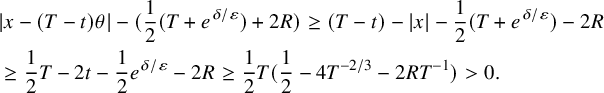 $$ \begin{align*} &|x-(T-t)\theta|-(\frac{1}{2}(T+e^{\delta/\varepsilon})+2R)\geq (T-t)-|x|-\frac{1}{2}(T+e^{\delta/\varepsilon})-2R\\ &\geq \frac{1}{2}T-2t-\frac{1}{2}e^{\delta/\varepsilon}-2R\geq \frac{1}{2}T(\frac{1}{2}-4T^{-2/3}-2RT^{-1})>0. \end{align*} $$
Thus, we have (5.3).
Next, we set $y=y(t,x,T,\theta )=x-(T-t)\theta $
. Since
$y=y(t,x,T,\theta )=x-(T-t)\theta $
. Since $T\gg t>|x|$
, we expect
$T\gg t>|x|$
, we expect $y\approx -T\theta $
. This expectation is made rigorous in the next lemma.
$y\approx -T\theta $
. This expectation is made rigorous in the next lemma.
Lemma 5.1. For all $t>(2e^{\delta /\varepsilon })^{1/3}$
,
$t>(2e^{\delta /\varepsilon })^{1/3}$
, $T=t^3$
,
$T=t^3$
, $|x|<t$
, and
$|x|<t$
, and $\theta \in \mathbb {S}^2$
, we have
$\theta \in \mathbb {S}^2$
, we have $|y|\sim T$
,
$|y|\sim T$
, $T-|y|=t+x\cdot \theta +O(t^{-1})\in [t-|x|-1,2t+1]$
, and
$T-|y|=t+x\cdot \theta +O(t^{-1})\in [t-|x|-1,2t+1]$
, and $y/|y|+\theta =O(t^{-2})$
.
$y/|y|+\theta =O(t^{-2})$
.
Proof. We have $||y|-(T-t)|\leq |x|$
. It follows that
$||y|-(T-t)|\leq |x|$
. It follows that
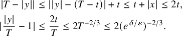 $$ \begin{align*} |T-|y||&\leq ||y|-(T-t)|+t\leq t+|x|\leq 2t,\\ |\frac{|y|}{T}-1|&\leq \frac{2t}{T}\leq 2T^{-2/3}\leq 2(e^{\delta/\varepsilon})^{-2/3}. \end{align*} $$
For $\varepsilon \ll _\delta 1$
, we have
$\varepsilon \ll _\delta 1$
, we have $(e^{\delta /\varepsilon })^{-2/3}=e^{-\frac {2\delta }{3\varepsilon }}<1/4$
, so
$(e^{\delta /\varepsilon })^{-2/3}=e^{-\frac {2\delta }{3\varepsilon }}<1/4$
, so $|y|\sim T$
.
$|y|\sim T$
.
Next, we have
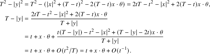 $$ \begin{align*} T^2-|y|^2&=T^2-(|x|^2+(T-t)^2-2(T-t)x\cdot\theta)=2tT-t^2-|x|^2+2(T-t)x\cdot\theta,\\ T-|y|&=\frac{2tT-t^2-|x|^2+2(T-t)x\cdot\theta}{T+|y|}\\ &=t+x\cdot\theta+\frac{t(T-|y|)-t^2-|x|^2+(T-|y|-2t)x\cdot\theta}{T+|y|}\\ &=t+x\cdot\theta+O(t^2/T)=t+x\cdot\theta+O(t^{-1}). \end{align*} $$
In the second last estimate, we use $|x|<t$
,
$|x|<t$
, $|T-|y||\leq 2t$
, and
$|T-|y||\leq 2t$
, and $|y|\sim T$
. It is also clear that
$|y|\sim T$
. It is also clear that $t-|x|-1\leq T-|y|\leq 2t+1$
.
$t-|x|-1\leq T-|y|\leq 2t+1$
.
Finally, we have
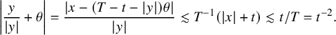 $$ \begin{align*} \left| \frac{y}{|y|}+\theta \right|&=\frac{|x-(T-t-|y|)\theta|}{|y|}\lesssim T^{-1}(|x|+t)\lesssim t/T=t^{-2}.\\[-41pt] \end{align*} $$
We can now compute $\Phi _I(T,y;\varepsilon )$
. For simplicity, in the remaining computations of the current subsection, we omit the parameter
$\Phi _I(T,y;\varepsilon )$
. For simplicity, in the remaining computations of the current subsection, we omit the parameter $\varepsilon $
in the functions
$\varepsilon $
in the functions $\Phi _I,u,\widetilde { u },A_I$
, etc. That is, we will only write
$\Phi _I,u,\widetilde { u },A_I$
, etc. That is, we will only write $\Phi _I(T,y)$
. Since
$\Phi _I(T,y)$
. Since $||y|-T|\lesssim t=T^{1/3}$
, by applying (3.14) with
$||y|-T|\lesssim t=T^{1/3}$
, by applying (3.14) with $N=|I|+2$
, for
$N=|I|+2$
, for $\varepsilon \ll _N1$
, we have
$\varepsilon \ll _N1$
, we have
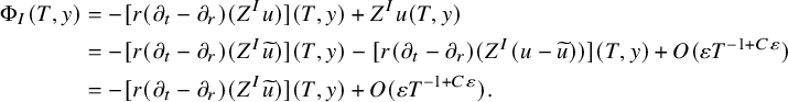 $$ \begin{align*} \Phi_I(T,y)&=-[r(\partial_t-\partial_r)(Z^Iu)](T,y)+Z^Iu(T,y)\\ &=-[r(\partial_t-\partial_r)(Z^I\widetilde{ u })](T,y)-[r(\partial_t-\partial_r)(Z^I(u-\widetilde{ u }))](T,y)+O(\varepsilon T^{-1+C\varepsilon})\\ &=-[r(\partial_t-\partial_r)(Z^I\widetilde{ u })](T,y)+O(\varepsilon T^{-1+C\varepsilon}). \end{align*} $$
Here, we use $|\partial Z^I(u-\widetilde { u })|\lesssim \langle r-t \rangle ^{-1}|Z Z^I(u-\widetilde { u })|$
to remove the
$|\partial Z^I(u-\widetilde { u })|\lesssim \langle r-t \rangle ^{-1}|Z Z^I(u-\widetilde { u })|$
to remove the $\langle r-t \rangle $
factor in (3.14). By Proposition 3.3, we have
$\langle r-t \rangle $
factor in (3.14). By Proposition 3.3, we have
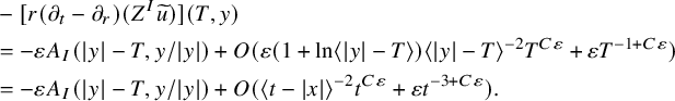 $$ \begin{align*} &-[r(\partial_t-\partial_r)(Z^I\widetilde{ u })](T,y)\\ &=-\varepsilon A_I(|y|-T,y/|y|)+O(\varepsilon (1+\ln\langle |y|-T \rangle)\langle |y|-T \rangle^{-2}T^{C\varepsilon}+\varepsilon T^{-1+C\varepsilon})\\ &=-\varepsilon A_I(|y|-T,y/|y|)+O(\langle t-|x| \rangle^{-2}t^{C\varepsilon}+\varepsilon t^{-3+C\varepsilon}). \end{align*} $$
In the last step, we use that $\varepsilon \ln \langle T-|y| \rangle \lesssim \varepsilon +\varepsilon \ln T\lesssim \varepsilon +\varepsilon \ln t\lesssim t^{C\varepsilon }$
and that
$\varepsilon \ln \langle T-|y| \rangle \lesssim \varepsilon +\varepsilon \ln T\lesssim \varepsilon +\varepsilon \ln t\lesssim t^{C\varepsilon }$
and that $\langle |y|-T \rangle ^{-2}\lesssim (1+t-|x|)^{-2}\lesssim \langle t-|x| \rangle ^{-2}$
by Lemma 5.1. Moreover, for
$\langle |y|-T \rangle ^{-2}\lesssim (1+t-|x|)^{-2}\lesssim \langle t-|x| \rangle ^{-2}$
by Lemma 5.1. Moreover, for $\rho $
lies between
$\rho $
lies between $|y|-T$
and
$|y|-T$
and $-t-x\cdot \theta $
,
$-t-x\cdot \theta $
,
 $$ \begin{align*} -\rho\geq \min\{T-|y|,t+x\cdot\theta\}\geq t+x\cdot\theta-Ct^{-1}\geq t-|x|-1>-1. \end{align*} $$
Thus, we have $\langle \rho \rangle \sim (2-\rho )\geq (t-|x|+1)\sim \langle t-|x| \rangle $
. By the mean value theorem, we have
$\langle \rho \rangle \sim (2-\rho )\geq (t-|x|+1)\sim \langle t-|x| \rangle $
. By the mean value theorem, we have
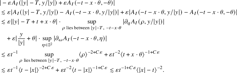 $$ \begin{align*} &|-\varepsilon A_I(|y|-T,y/|y|)+\varepsilon A_I(-t-x\cdot\theta,-\theta)|\\ &\lesssim \varepsilon|A_I(|y|-T,y/|y|)- A_I(-t-x\cdot\theta,y/|y|)|+\varepsilon|A_I(-t-x\cdot \theta,y/|y|)- A_I(-t-x\cdot\theta,-\theta)|\\ &\lesssim\varepsilon||y|-T+t+x\cdot\theta|\cdot \sup_{\rho\ \text{lies between }|y|-T,\ -t-x\cdot\theta}|\partial_qA_I(\rho,y/|y|)|\\ &\quad+\varepsilon|\frac{y}{|y|}+\theta|\cdot \sup_{\eta\in\mathbb{S}^2}|\partial_\omega A_I(-t-x\cdot\theta,\eta)|\\ &\lesssim\varepsilon t^{-1}\sup_{\rho\ \text{lies between }|y|-T,\ -t-x\cdot\theta}\langle \rho \rangle^{-2+C\varepsilon}+\varepsilon t^{-2}\langle t+x\cdot\theta \rangle^{-1+C\varepsilon}\\ &\lesssim \varepsilon t^{-1}\langle t-|x| \rangle^{-2+C\varepsilon}+\varepsilon t^{-2}\langle t-|x| \rangle^{-1+C\varepsilon}\lesssim \varepsilon t^{-1+C\varepsilon}\langle |x|-t \rangle^{-2}. \end{align*} $$
In summary, we have
 $$ \begin{align*} \Phi_I(T,y;\varepsilon)&=-\varepsilon A_I(-t-x\cdot\theta,-\theta;\varepsilon)+O(\langle r-t \rangle^{-2}t^{C\varepsilon}). \end{align*} $$
Plugging this back to (5.2), we obtain
 $$ \begin{align}\begin{aligned} Z^Iu(t,x;\varepsilon)&=-\frac{\varepsilon }{4\pi}\int_{\mathbb{S}^2} A_I(-t+x\cdot\theta,\theta;\varepsilon)\ dS_\theta+O(\langle t-|x| \rangle^{-2}t^{C\varepsilon}),\ \forall t>(2e^{\delta/\varepsilon})^{1/3},\ |x|<t. \end{aligned}\end{align} $$
6 Corollaries of Theorem 1
Combining Theorem 1 with the asymptotic completeness result for (1.1), we can prove several interesting corollaries.
In Section 6.1, we show a special decaying property for $\widehat { A }$
and
$\widehat { A }$
and $\widehat { U }$
; see (6.2) in Proposition 6.1. In the proof, we compute the integral
$\widehat { U }$
; see (6.2) in Proposition 6.1. In the proof, we compute the integral $\int _{\mathbb {S}^2}u(t,(t-t^{2/3})\omega )\ dS_\omega $
in two ways. First, we can use the estimates from the asymptotic completeness result. By (3.14) and Proposition 3.3, we have
$\int _{\mathbb {S}^2}u(t,(t-t^{2/3})\omega )\ dS_\omega $
in two ways. First, we can use the estimates from the asymptotic completeness result. By (3.14) and Proposition 3.3, we have
 $$ \begin{align*} \int_{\mathbb{S}^2}u(t,(t-t^{2/3})\omega)\ dS_\omega\approx \varepsilon (t-t^{2/3})^{-1}\cdot\int_{\mathbb{S}^2}\widehat{ U }(\varepsilon\ln t-\delta,-t^{2/3},\omega)\ dS_\omega,\qquad \forall t\gg_{\delta,\varepsilon}1. \end{align*} $$
Meanwhile, we can apply the main theorem for this paper. By (1.23), we have
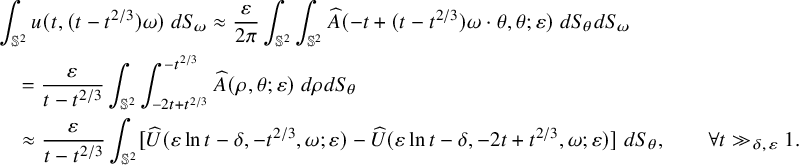 $$ \begin{align*} &\int_{\mathbb{S}^2}u(t,(t-t^{2/3})\omega)\ dS_\omega\approx \frac{\varepsilon}{2\pi} \int_{\mathbb{S}^2}\int_{\mathbb{S}^2}\widehat{ A }(-t+(t-t^{2/3})\omega\cdot\theta,\theta;\varepsilon)\ dS_\theta dS_\omega\\&\quad=\frac{\varepsilon}{t-t^{2/3}} \int_{\mathbb{S}^2}\int_{-2t+t^{2/3}}^{-t^{2/3}}\widehat{ A }(\rho,\theta;\varepsilon)\ d\rho dS_\theta\\&\quad\approx\frac{\varepsilon}{t-t^{2/3}} \int_{\mathbb{S}^2}[\widehat{ U }(\varepsilon\ln t-\delta,-t^{2/3},\omega;\varepsilon)-\widehat{ U }(\varepsilon\ln t-\delta,-2t+t^{2/3},\omega;\varepsilon)]\ dS_\theta,\qquad \forall t\gg_{\delta,\varepsilon}1. \end{align*} $$
In the second step, we integrate with respect to $\omega $
. In the last step, we notice that
$\omega $
. In the last step, we notice that $\widehat { U }_q\approx \widehat { A }$
. Comparing these two approximate identities, we notice that there is a cancellation. We thus have
$\widehat { U }_q\approx \widehat { A }$
. Comparing these two approximate identities, we notice that there is a cancellation. We thus have
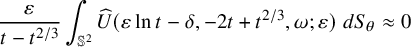 $$ \begin{align*} \frac{\varepsilon}{t-t^{2/3}} \int_{\mathbb{S}^2} \widehat{ U }(\varepsilon\ln t-\delta,-2t+t^{2/3},\omega;\varepsilon)\ dS_\theta\approx 0 \end{align*} $$
to some extent. For simplicity, we skip the discussion on how to control the error terms in these computations, and we refer to the proof of Proposition 6.1 below. Following the same idea, one can derive similar decay properties for the $U_I$
’s defined in Proposition 3.3; see (6.1).
$U_I$
’s defined in Proposition 3.3; see (6.1).
In Sections 6.2 and 6.3, we prove Theorems 2 and 3. Here, Proposition 6.2 is the same as Theorem 2, while Proposition 6.6 is slightly stronger than Theorem 3. Note that the ideas of the proofs of Propositions 6.2 and 6.6 have been explained in the introduction, so we will not repeat them here.
6.1 Decaying properties of the
$U_I$
’s

We now discuss the decaying properties mentioned at the beginning of this section.
Proposition 6.1. For each multiindex I, we let $U_I$
be the function of
$U_I$
be the function of $(s,q,\omega )$
defined in the statement of Proposition 3.3. Then, for all
$(s,q,\omega )$
defined in the statement of Proposition 3.3. Then, for all $t\geq 2e^{\delta /\varepsilon }$
, we have
$t\geq 2e^{\delta /\varepsilon }$
, we have
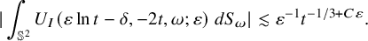 $$ \begin{align}\begin{aligned} |\int_{\mathbb{S}^2}U_I(\varepsilon\ln t-\delta,-2t,\omega;\varepsilon)\ dS_\omega|\lesssim\varepsilon^{-1}t^{-1/3+C\varepsilon}. \end{aligned}\end{align} $$
In particular, since $U_0=\widehat { U }$
which was defined in (3.16), we have
$U_0=\widehat { U }$
which was defined in (3.16), we have
 $$ \begin{align}\begin{aligned} |\int_{\mathbb{S}^2}\int_{-2t}^R\widehat{ A }(q,\omega;\varepsilon)\exp(\frac{1}{2}G(\omega)\widehat{ A }(q,\omega;\varepsilon)\cdot(\varepsilon\ln t-\delta))\ dqdS_\omega|\lesssim\varepsilon^{-1}t^{-1/3+C\varepsilon}. \end{aligned}\end{align} $$
Proof. Fix a constant $\gamma \in (0,1)$
. For each
$\gamma \in (0,1)$
. For each $(t,x)\in \Omega \cap \{-2t^\gamma <r-t<-t^\gamma /2\}$
, we have two ways to approximate
$(t,x)\in \Omega \cap \{-2t^\gamma <r-t<-t^\gamma /2\}$
, we have two ways to approximate $Z^Iu$
. By (3.14) and Proposition 3.3, we have
$Z^Iu$
. By (3.14) and Proposition 3.3, we have
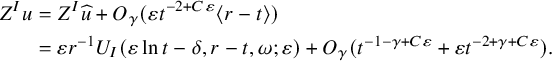 $$ \begin{align*} Z^Iu&=Z^I\widehat{ u }+O_\gamma(\varepsilon t^{-2+C\varepsilon}\langle r-t \rangle)\\ &=\varepsilon r^{-1}U_I(\varepsilon\ln t-\delta,r-t,\omega;\varepsilon)+O_\gamma(t^{-1-\gamma+ C\varepsilon}+\varepsilon t^{-2+\gamma+C\varepsilon}). \end{align*} $$
Here, we use $|r-t|\sim t^{\gamma }$
. Meanwhile, by Theorem 1, we have
$|r-t|\sim t^{\gamma }$
. Meanwhile, by Theorem 1, we have
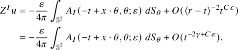 $$ \begin{align*} Z^Iu&=-\frac{\varepsilon}{4\pi}\int_{\mathbb{S}^2}A_I(-t+x\cdot\theta,\theta;\varepsilon)\ dS_\theta+O(\langle r-t \rangle^{-2}t^{C\varepsilon})\\ &=-\frac{\varepsilon}{4\pi}\int_{\mathbb{S}^2}A_I(-t+x\cdot\theta,\theta;\varepsilon)\ dS_\theta+O(t^{-2\gamma+C\varepsilon}). \end{align*} $$
By combining these two estimates, we have
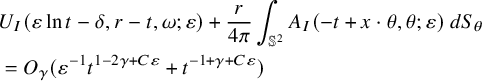 $$ \begin{align}\begin{aligned} &U_I(\varepsilon\ln t-\delta,r-t,\omega;\varepsilon)+\frac{r}{4\pi}\int_{\mathbb{S}^2}A_I(-t+x\cdot\theta,\theta;\varepsilon)\ dS_\theta\\ &=O_\gamma(\varepsilon^{-1}t^{1-2\gamma+ C\varepsilon}+ t^{-1+\gamma+C\varepsilon}) \end{aligned}\end{align} $$
whenever $(t,x)\in \Omega $
and
$(t,x)\in \Omega $
and $-2t^\gamma <r-t<-t^\gamma /2$
.
$-2t^\gamma <r-t<-t^\gamma /2$
.
To continue, we let $t>2e^{\delta /\varepsilon }$
and
$t>2e^{\delta /\varepsilon }$
and $r=t-t^{2/3}$
in (6.3). Note that
$r=t-t^{2/3}$
in (6.3). Note that $\max \{1-2\gamma ,-1+\gamma \}$
from the power of t in (6.3) is minimized at
$\max \{1-2\gamma ,-1+\gamma \}$
from the power of t in (6.3) is minimized at $\gamma =2/3$
. Moreover, we have
$\gamma =2/3$
. Moreover, we have
 $$ \begin{align*} r-(t+e^{\delta/\varepsilon})/2-2R=(t-e^{\delta/\varepsilon})/2-t^{2/3}-2R>t/4-t^{2/3}-2R>0, \end{align*} $$
so $\{t>2e^{\delta /\varepsilon },r=t-t^{2/3}\}\subset \Omega $
. This gives us
$\{t>2e^{\delta /\varepsilon },r=t-t^{2/3}\}\subset \Omega $
. This gives us
 $$ \begin{align*} U_I(\varepsilon\ln t-\delta,-t^{2/3},\omega;\varepsilon)+\frac{r}{4\pi}\int_{\mathbb{S}^2}A_I(-t+r\omega\cdot\theta,\theta;\varepsilon)\ dS_\theta=O(\varepsilon^{-1}t^{-1/3+ C\varepsilon}). \end{align*} $$
Integrate both sides with respect to $\omega $
on
$\omega $
on $\mathbb {S}^2$
, and we get
$\mathbb {S}^2$
, and we get
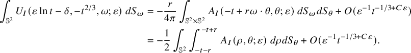 $$ \begin{align*} \int_{\mathbb{S}^2}U_I(\varepsilon\ln t-\delta,-t^{2/3},\omega;\varepsilon)\ dS_\omega&=-\frac{r}{4\pi}\int_{\mathbb{S}^2\times\mathbb{S}^2}A_I(-t+r\omega\cdot\theta,\theta;\varepsilon)\ dS_\omega dS_\theta+O(\varepsilon^{-1}t^{-1/3+ C\varepsilon})\\ &=-\frac{1}{2}\int_{\mathbb{S}^2}\int_{-t-r}^{-t+r}A_I(\rho,\theta;\varepsilon)\ d\rho dS_\theta+O(\varepsilon^{-1}t^{-1/3+ C\varepsilon}). \end{align*} $$
Note that
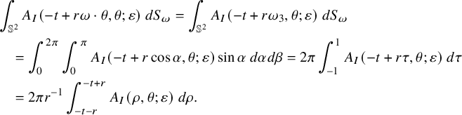 $$ \begin{align}\begin{aligned} &\int_{\mathbb{S}^2}A_I(-t+r\omega\cdot\theta,\theta;\varepsilon)\ dS_\omega =\int_{\mathbb{S}^2}A_I(-t+r\omega_3,\theta;\varepsilon)\ dS_\omega\\&\quad=\int_0^{2\pi}\int_{0}^\pi A_I(-t+r\cos\alpha,\theta;\varepsilon)\sin\alpha\ d\alpha d\beta=2\pi \int_{-1}^1A_I(-t+r\tau,\theta;\varepsilon)\ d\tau\\&\quad=2\pi r^{-1} \int_{-t-r}^{-t+r}A_I(\rho,\theta;\varepsilon)\ d\rho. \end{aligned}\end{align} $$
In the first step, we notice that the integral is invariant under rotation. In the second step, we write the integral in the spherical coordinates. Moreover, recall from (3.29) that $2\partial _qU_I+A_I=O(\langle q \rangle ^{-2+C\varepsilon }e^{Cs})$
, so we have (recall that
$2\partial _qU_I+A_I=O(\langle q \rangle ^{-2+C\varepsilon }e^{Cs})$
, so we have (recall that $r-t=-t^{2/3}$
)
$r-t=-t^{2/3}$
)
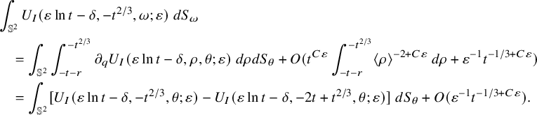 $$ \begin{align*} &\int_{\mathbb{S}^2}U_I(\varepsilon\ln t-\delta,-t^{2/3},\omega;\varepsilon)\ dS_\omega\\&\quad=\int_{\mathbb{S}^2}\int_{-t-r}^{-t^{2/3}}\partial_qU_I(\varepsilon\ln t-\delta,\rho,\theta;\varepsilon)\ d\rho dS_\theta+O(t^{C\varepsilon}\int_{-t-r}^{-t^{2/3}}\langle \rho \rangle^{-2+C\varepsilon}\ d\rho+\varepsilon^{-1}t^{-1/3+ C\varepsilon})\\&\quad=\int_{\mathbb{S}^2}[U_I(\varepsilon\ln t-\delta,-t^{2/3},\theta;\varepsilon)-U_I(\varepsilon\ln t-\delta,-2t+t^{2/3},\theta;\varepsilon)]\ dS_\theta+O(\varepsilon^{-1}t^{-1/3+ C\varepsilon}). \end{align*} $$
It follows that
 $$ \begin{align*} \int_{\mathbb{S}^2} U_I(\varepsilon\ln t-\delta,-2t+t^{2/3},\theta;\varepsilon)\ dS_\theta=O(\varepsilon^{-1}t^{-1/3+C\varepsilon}),\qquad \forall t\geq 2e^{\delta/\varepsilon}. \end{align*} $$
Finally, by (3.27), we have $\partial _qU_I=O(\langle q \rangle ^{-1+C\varepsilon }e^{Cs})$
. By the mean value theorem, we have
$\partial _qU_I=O(\langle q \rangle ^{-1+C\varepsilon }e^{Cs})$
. By the mean value theorem, we have
 $$ \begin{align*} |U_I(\varepsilon\ln t-\delta,-2t+t^{2/3},\theta;\varepsilon)-U_I(\varepsilon\ln t-\delta,-2t,\theta;\varepsilon)|\lesssim t^{-1+C\varepsilon}\cdot t^{2/3}\lesssim t^{-1/3+C\varepsilon}.\\[-37pt] \end{align*} $$
Remark 6.1.1. Let us compare (6.1) with the pointwise bounds for $U_I$
obtained in Proposition 3.3. There it was proved that for all
$U_I$
obtained in Proposition 3.3. There it was proved that for all $(s,q,\omega )\in [0,\infty )\times \mathbb {R}\times \mathbb {S}^2$
, we have
$(s,q,\omega )\in [0,\infty )\times \mathbb {R}\times \mathbb {S}^2$
, we have $U_I=O(\varepsilon ^{-1}\langle q \rangle ^{C\varepsilon }e^{Cs})$
. Thus, we have
$U_I=O(\varepsilon ^{-1}\langle q \rangle ^{C\varepsilon }e^{Cs})$
. Thus, we have
 $$ \begin{align*} |U_I(\varepsilon\ln t-\delta,-2t,\omega;\varepsilon)|\lesssim \varepsilon^{-1}t^{C\varepsilon},\qquad \forall t\geq 2e^{\delta/\varepsilon},\omega\in\mathbb{S}^2. \end{align*} $$
The estimate (6.1), however, indicates that
 $$ \begin{align*} \inf_{\omega\in\mathbb{S}^2}|U_I(\varepsilon\ln t-\delta,-2t,\omega;\varepsilon)|\lesssim \varepsilon^{-1}t^{-1/3+C\varepsilon},\qquad\forall t\geq 2e^{\delta/\varepsilon}. \end{align*} $$
6.2 Sufficient conditions for vanishing
$\widehat { A }$

We can now prove Theorem 2.
Proposition 6.2. Suppose that the quasilinear wave equation (1.1) violates the null condition. That is, we have $G(\omega )\not \equiv 0$
on
$G(\omega )\not \equiv 0$
on $\mathbb {S}^2$
, or equivalently,
$\mathbb {S}^2$
, or equivalently, $g^{\alpha \beta }_0\neq 0$
for some
$g^{\alpha \beta }_0\neq 0$
for some $\alpha ,\beta =0,1,2,3$
. Fix
$\alpha ,\beta =0,1,2,3$
. Fix $(u_0,u_1)\in C_c^\infty (\mathbb {R}^3)$
and
$(u_0,u_1)\in C_c^\infty (\mathbb {R}^3)$
and $0<\varepsilon \ll 1$
. Let u be the global
$0<\varepsilon \ll 1$
. Let u be the global $C^\infty $
solution to (1.1) with data
$C^\infty $
solution to (1.1) with data $(\varepsilon u_0,\varepsilon u_1)$
. Fix
$(\varepsilon u_0,\varepsilon u_1)$
. Fix $\delta \in (0,1)$
and let
$\delta \in (0,1)$
and let $\widehat { A }$
be the corresponding function defined by (3.16) in the asymptotic completeness result in Section 3.
$\widehat { A }$
be the corresponding function defined by (3.16) in the asymptotic completeness result in Section 3.
Moreover, suppose that one of the following assumptions holds:
-
a) We have
$\min _{(q,\omega )\in \mathbb {R}\times \mathbb {S}^2}\widehat { A }(q,\omega ;\varepsilon )\geq 0$
or
$\max _{(q,\omega )\in \mathbb {R}\times \mathbb {S}^2}\widehat { A }(q,\omega ;\varepsilon )\leq 0$
; -
b) We have
$\min _{ \omega \in \mathbb {S}^2}G(\omega )\geq 0$
and
$\min \{\widehat { A },0\}\in L^1_{q,\omega }(\mathbb {R}\times \mathbb {S}^2)$
, or we have
$\max _{ \omega \in \mathbb {S}^2}G(\omega )\leq 0$
and
$\max \{\widehat { A },0\}\in L^1_{q,\omega }(\mathbb {R}\times \mathbb {S}^2)$
; -
c) Let
$C_0>0$
be a constant uniform in all
$\varepsilon \ll 1$
such that Suppose that there exists a constant
$$ \begin{align*} C_0\geq \sup_{(q,\omega)\in\mathbb{R}\times\mathbb{S}^2}|\frac{1}{2} G(\omega)\widehat{ A }(q,\omega;\varepsilon)|. \end{align*} $$
$B_0>C_0$
that is also uniform in all
$\varepsilon \ll 1$
, such that
$$ \begin{align*} \lim_{q\to-\infty}\langle q \rangle^{1+B_0\varepsilon}\sup_{\omega\in\mathbb{S}^2}|\widehat{ A }(q,\omega;\varepsilon)|=0. \end{align*} $$


Then, as long as $\varepsilon \ll 1$
(depending on the constant
$\varepsilon \ll 1$
(depending on the constant $B_0$
in part c)), we have
$B_0$
in part c)), we have $\widehat { A }\equiv 0$
and thus
$\widehat { A }\equiv 0$
and thus $u\equiv 0$
.
$u\equiv 0$
.
To prove Proposition 6.2, we will first prove that if one of the assumptions a), b) and c) holds, then we have $\widehat { A }\equiv 0$
. We will then show that
$\widehat { A }\equiv 0$
. We will then show that $u\equiv 0$
if
$u\equiv 0$
if $\widehat { A }\equiv 0$
.
$\widehat { A }\equiv 0$
.
6.2.1 The assumption a)
Assume that $\min _{(q,\omega )\in \mathbb {R}\times \mathbb {S}^2}\widehat { A }(q,\omega ;\varepsilon )\geq 0$
or
$\min _{(q,\omega )\in \mathbb {R}\times \mathbb {S}^2}\widehat { A }(q,\omega ;\varepsilon )\geq 0$
or $\max _{(q,\omega )\in \mathbb {R}\times \mathbb {S}^2}\widehat { A }(q,\omega ;\varepsilon )\leq 0$
. Now, we can rewrite (6.2) as
$\max _{(q,\omega )\in \mathbb {R}\times \mathbb {S}^2}\widehat { A }(q,\omega ;\varepsilon )\leq 0$
. Now, we can rewrite (6.2) as
 $$ \begin{align*} \int_{\mathbb{S}^2}\!\int_{\mathbb{R}}\! 1_{q\in[-2t,R]}\cdot |\widehat{ A }(q,\omega;\varepsilon)|\exp(\frac{1}{2}G(\omega)\widehat{ A }(q,\omega;\varepsilon)\cdot (\varepsilon\ln t-\delta))\ dqdS_\omega\lesssim \varepsilon^{-1}t^{-1/3+C\varepsilon},\ \forall t\geq 2e^{\delta/\varepsilon}. \end{align*} $$
Here the integrand is nonnegative everywhere. Besides, we have
 $$ \begin{align*} \exp(\frac{1}{2}G(\omega)\widehat{ A }(q,\omega;\varepsilon)\cdot (\varepsilon\ln t-\delta))\geq \exp(-C(\varepsilon\ln t-\delta))\gtrsim t^{-C\varepsilon}. \end{align*} $$
As a result, we have
 $$ \begin{align*} \int_{\mathbb{S}^2}\int_{\mathbb{R}}1_{q\in[-2t,R]}\cdot |\widehat{ A }(q,\omega;\varepsilon)|\ dqdS_\omega\lesssim \varepsilon^{-1}t^{-1/3+C\varepsilon}\cdot t^{C\varepsilon},\qquad\forall t\geq 2e^{\delta/\varepsilon}. \end{align*} $$
We send $t\to \infty $
and apply the monotone convergence theorem. As long as
$t\to \infty $
and apply the monotone convergence theorem. As long as $\varepsilon \ll 1$
, we have
$\varepsilon \ll 1$
, we have $t^{-1/3+C\varepsilon }\cdot t^{C\varepsilon }\leq t^{-1/6}$
. This yields
$t^{-1/3+C\varepsilon }\cdot t^{C\varepsilon }\leq t^{-1/6}$
. This yields
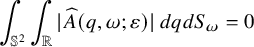 $$ \begin{align*} \int_{\mathbb{S}^2}\int_{\mathbb{R}} |\widehat{ A }(q,\omega;\varepsilon)|\ dqdS_\omega=0 \end{align*} $$
and thus $\widehat { A }=0$
almost everywhere. Since
$\widehat { A }=0$
almost everywhere. Since $\widehat { A }$
is continuous, we conclude that
$\widehat { A }$
is continuous, we conclude that $\widehat { A }\equiv 0$
.
$\widehat { A }\equiv 0$
.
6.2.2 The assumption b)
Assume that $\min _{ \omega \in \mathbb {S}^2}G(\omega )\geq 0$
and
$\min _{ \omega \in \mathbb {S}^2}G(\omega )\geq 0$
and $\min \{\widehat { A },0\}\in L^1_{q,\omega }(\mathbb {R}\times \mathbb {S}^2)$
. Or, assume that
$\min \{\widehat { A },0\}\in L^1_{q,\omega }(\mathbb {R}\times \mathbb {S}^2)$
. Or, assume that $\max _{ \omega \in \mathbb {S}^2}G(\omega )\leq 0$
and
$\max _{ \omega \in \mathbb {S}^2}G(\omega )\leq 0$
and $\max \{\widehat { A },0\}\in L^1_{q,\omega }(\mathbb {R}\times \mathbb {S}^2)$
. We now set
$\max \{\widehat { A },0\}\in L^1_{q,\omega }(\mathbb {R}\times \mathbb {S}^2)$
. We now set
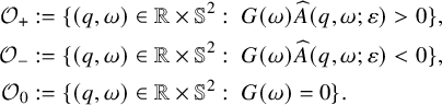 $$ \begin{align*} \mathcal{ O }_+&:=\{(q,\omega)\in\mathbb{R}\times\mathbb{S}^2:\ G(\omega)\widehat{ A }(q,\omega;\varepsilon)>0\},\\ \mathcal{ O }_-&:=\{(q,\omega)\in\mathbb{R}\times\mathbb{S}^2:\ G(\omega)\widehat{ A }(q,\omega;\varepsilon)<0\},\\ \mathcal{ O }_0&:=\{(q,\omega)\in\mathbb{R}\times\mathbb{S}^2:\ G(\omega)=0\}. \end{align*} $$
Note that $\widehat { A }=0$
in
$\widehat { A }=0$
in $(\mathbb {R}\times \mathbb {S}^2)\setminus (\mathcal { O }_+\cup \mathcal { O }_-\cup \mathcal { O }_0)$
and that
$(\mathbb {R}\times \mathbb {S}^2)\setminus (\mathcal { O }_+\cup \mathcal { O }_-\cup \mathcal { O }_0)$
and that $\mathcal { O }_+,\mathcal { O }_-,\mathcal { O }_0$
are pairwise disjoint. Thus, we can write the integral on the left-hand side of (6.2) as the sum of
$\mathcal { O }_+,\mathcal { O }_-,\mathcal { O }_0$
are pairwise disjoint. Thus, we can write the integral on the left-hand side of (6.2) as the sum of
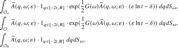 $$ \begin{align*} &\int_{\mathcal{ O }_+}\widehat{ A }(q,\omega;\varepsilon)\cdot 1_{q\in[-2t,R]}\cdot\exp(\frac{1}{2}G(\omega)\widehat{ A }(q,\omega;\varepsilon)\cdot(\varepsilon\ln t-\delta))\ dqdS_\omega,\\ &\int_{\mathcal{ O }_-}\widehat{ A }(q,\omega;\varepsilon)\cdot 1_{q\in[-2t,R]}\cdot\exp(\frac{1}{2}G(\omega)\widehat{ A }(q,\omega;\varepsilon)\cdot(\varepsilon\ln t-\delta))\ dqdS_\omega,\\ &\int_{\mathcal{ O }_0}\widehat{ A }(q,\omega;\varepsilon)\cdot 1_{q\in[-2t,R]}\ dqdS_\omega. \end{align*} $$
Since $G(\omega )\not \equiv 0$
on
$G(\omega )\not \equiv 0$
on $\mathbb {S}^2$
, the set
$\mathbb {S}^2$
, the set $\{\omega \in \mathbb {S}^2:\ G(\omega )=0\}$
has surface measure
$\{\omega \in \mathbb {S}^2:\ G(\omega )=0\}$
has surface measure $0$
. Thus, the last integral equals zero.
$0$
. Thus, the last integral equals zero.
If $\min _{\omega \in \mathbb {S}^2}G(\omega )\geq 0$
, we have
$\min _{\omega \in \mathbb {S}^2}G(\omega )\geq 0$
, we have $\widehat { A }|_{\mathcal { O }_+}>0$
and
$\widehat { A }|_{\mathcal { O }_+}>0$
and $\widehat { A }|_{\mathcal { O }_-}<0$
. If
$\widehat { A }|_{\mathcal { O }_-}<0$
. If $\max _{\omega \in \mathbb {S}^2}G(\omega )\leq 0$
, we have
$\max _{\omega \in \mathbb {S}^2}G(\omega )\leq 0$
, we have $\widehat { A }|_{\mathcal { O }_-}>0$
and
$\widehat { A }|_{\mathcal { O }_-}>0$
and $\widehat { A }|_{\mathcal { O }_+}<0$
. Thus, by (6.2), we have for all
$\widehat { A }|_{\mathcal { O }_+}<0$
. Thus, by (6.2), we have for all $t\geq 2t^{\delta /\varepsilon }$
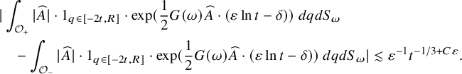 $$ \begin{align*} &|\int_{\mathcal{ O }_+}|\widehat{ A }|\cdot 1_{q\in[-2t,R]}\cdot\exp(\frac{1}{2}G(\omega)\widehat{ A } \cdot(\varepsilon\ln t-\delta))\ dqdS_\omega\\ &\quad-\int_{\mathcal{ O }_-}|\widehat{ A }|\cdot 1_{q\in[-2t,R]}\cdot\exp(\frac{1}{2}G(\omega)\widehat{ A } \cdot(\varepsilon\ln t-\delta))\ dqdS_\omega|\lesssim \varepsilon^{-1}t^{-1/3+C\varepsilon}. \end{align*} $$
Under the assumption b), we have $\widehat { A }\cdot 1_{\mathcal { O }_-}=\widehat { A }\cdot 1_{G(\omega )\widehat { A }<0}\in L^{1}_{q,\omega }$
. Moreover, we have
$\widehat { A }\cdot 1_{\mathcal { O }_-}=\widehat { A }\cdot 1_{G(\omega )\widehat { A }<0}\in L^{1}_{q,\omega }$
. Moreover, we have $1\geq \exp (\frac {1}{2}G(\omega )\widehat { A } \cdot (\varepsilon \ln t-\delta ))\to 0$
as
$1\geq \exp (\frac {1}{2}G(\omega )\widehat { A } \cdot (\varepsilon \ln t-\delta ))\to 0$
as $t\to \infty $
in
$t\to \infty $
in $\mathcal { O }_-$
. Thus, by the Lebesgue dominated convergence theorem, we conclude that
$\mathcal { O }_-$
. Thus, by the Lebesgue dominated convergence theorem, we conclude that
 $$ \begin{align*} \int_{\mathcal{ O }_-}|\widehat{ A }|\cdot 1_{q\in[-2t,R]}\cdot\exp(\frac{1}{2}G(\omega)\widehat{ A } \cdot(\varepsilon\ln t-\delta))\ dqdS_\omega\to 0,\qquad \text{as }t\to\infty. \end{align*} $$
As a result, we have
 $$ \begin{align*} \int_{\mathcal{ O }_+}|\widehat{ A }|\cdot 1_{q\in[-2t,R]}\cdot\exp(\frac{1}{2}G(\omega)\widehat{ A } \cdot(\varepsilon\ln t-\delta))\ dqdS_\omega\to 0,\qquad \text{as }t\to\infty. \end{align*} $$
However, since $G(\omega )\widehat { A }>0$
in
$G(\omega )\widehat { A }>0$
in $\mathcal { O }_+$
, by the monotone convergence theorem, we have
$\mathcal { O }_+$
, by the monotone convergence theorem, we have
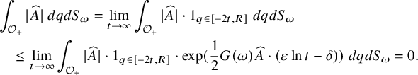 $$ \begin{align*} &\int_{\mathcal{ O }_+}|\widehat{ A }|\ dqdS_\omega=\lim_{t\to\infty}\int_{\mathcal{ O }_+}|\widehat{ A }|\cdot 1_{q\in[-2t,R]}\ dqdS_\omega\\&\quad \leq \lim_{t\to\infty}\int_{\mathcal{ O }_+}|\widehat{ A }|\cdot 1_{q\in[-2t,R]}\cdot\exp(\frac{1}{2}G(\omega)\widehat{ A } \cdot(\varepsilon\ln t-\delta))\ dqdS_\omega=0. \end{align*} $$
It follows that $\widehat { A }=0$
almost everywhere in
$\widehat { A }=0$
almost everywhere in $\mathcal { O }_+$
. But the definition of
$\mathcal { O }_+$
. But the definition of $\mathcal { O }_+$
implies that
$\mathcal { O }_+$
implies that $\widehat { A }\neq 0$
in
$\widehat { A }\neq 0$
in $\mathcal { O }_+$
. Thus,
$\mathcal { O }_+$
. Thus, $\mathcal { O }_+$
has zero measure in
$\mathcal { O }_+$
has zero measure in $\mathbb {R}\times \mathbb {S}^2$
. By (6.2) again, we have
$\mathbb {R}\times \mathbb {S}^2$
. By (6.2) again, we have
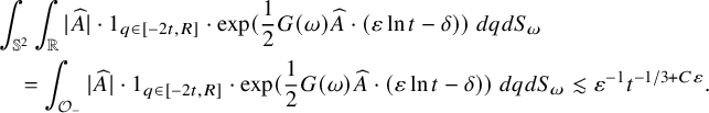 $$ \begin{align*} &\int_{\mathbb{S}^2}\int_{\mathbb{R}}|\widehat{ A }|\cdot 1_{q\in[-2t,R]}\cdot\exp(\frac{1}{2}G(\omega)\widehat{ A } \cdot(\varepsilon\ln t-\delta))\ dqdS_\omega\\&\quad=\int_{\mathcal{ O }_-}|\widehat{ A }|\cdot 1_{q\in[-2t,R]}\cdot\exp(\frac{1}{2}G(\omega)\widehat{ A } \cdot(\varepsilon\ln t-\delta))\ dqdS_\omega\lesssim \varepsilon^{-1}t^{-1/3+C\varepsilon}. \end{align*} $$
Following the proof in Section 6.2.1, we conclude that $\widehat { A }\equiv 0$
.
$\widehat { A }\equiv 0$
.
6.2.3 The assumption c)
Let $C_0>0$
be a constant uniform in all
$C_0>0$
be a constant uniform in all $\varepsilon \ll 1$
such that
$\varepsilon \ll 1$
such that
 $$ \begin{align*} C_0\geq \sup_{(q,\omega)\in\mathbb{R}\times\mathbb{S}^2}|\frac{1}{2} G(\omega)\widehat{ A }(q,\omega;\varepsilon)|. \end{align*} $$
Such a $C_0$
exists because we have
$C_0$
exists because we have $|\widehat { A }|\lesssim \langle q \rangle ^{-1+C\varepsilon }$
with an implicit constant uniform in
$|\widehat { A }|\lesssim \langle q \rangle ^{-1+C\varepsilon }$
with an implicit constant uniform in $\varepsilon \ll 1$
. Suppose that there exists a constant
$\varepsilon \ll 1$
. Suppose that there exists a constant $B_0>C_0$
that is also uniform in all
$B_0>C_0$
that is also uniform in all $\varepsilon \ll 1$
, such that
$\varepsilon \ll 1$
, such that
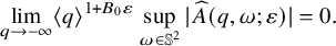 $$ \begin{align*} \lim_{q\to-\infty}\langle q \rangle^{1+B_0\varepsilon}\sup_{\omega\in\mathbb{S}^2}|\widehat{ A }(q,\omega;\varepsilon)|=0. \end{align*} $$
Recall that $\widehat { A }$
is a continuous function and that
$\widehat { A }$
is a continuous function and that $\widehat { A }|_{q\geq R}\equiv 0$
. From this limit, we have
$\widehat { A }|_{q\geq R}\equiv 0$
. From this limit, we have
 $$ \begin{align}\begin{aligned} |\widehat{ A }(q,\omega;\varepsilon)|&\lesssim_{B_0,\varepsilon}\langle q \rangle^{-1-B_0\varepsilon},\qquad \forall (q,\omega)\in\mathbb{R}\times\mathbb{S}^2. \end{aligned}\end{align} $$
The implicit constant in (6.5) is allowed to depend on $\varepsilon $
. We remark that this implicit constant is not important in our proof for part c).
$\varepsilon $
. We remark that this implicit constant is not important in our proof for part c).
We now derive a pointwise decay for u from (6.5). Recall that (5.4) with $|I|=0$
yields
$|I|=0$
yields
 $$ \begin{align*} u(t,x;\varepsilon)&=\frac{\varepsilon }{2\pi}\int_{\mathbb{S}^2} \widehat{ A }(-t+x\cdot\theta,\theta;\varepsilon)\ dS_\theta+O(\langle t-|x| \rangle^{-2}t^{C\varepsilon}) \end{align*} $$
whenever $t\geq (2e^{\delta /\varepsilon })^{1/3}$
and
$t\geq (2e^{\delta /\varepsilon })^{1/3}$
and $|x|<t$
.
$|x|<t$
.
Lemma 6.3. Fix $\nu _0\in (1/2,1)$
. Then, for all
$\nu _0\in (1/2,1)$
. Then, for all $(t,x)\in \mathbb {R}^{1+3}$
with
$(t,x)\in \mathbb {R}^{1+3}$
with $t\geq (2e^{\delta /\varepsilon })^{1/3}$
and
$t\geq (2e^{\delta /\varepsilon })^{1/3}$
and $|x|\leq t-t^{\nu _0}/2$
, we have
$|x|\leq t-t^{\nu _0}/2$
, we have
 $$ \begin{align*} |u(t,x)|&\lesssim_{\varepsilon,B_0,\nu_0}t^{-1}\langle |x|-t \rangle^{-B_0\varepsilon} \end{align*} $$
as long as $\varepsilon \ll _{B_0,\nu _0}1$
.
$\varepsilon \ll _{B_0,\nu _0}1$
.
Proof. We first estimate the spherical integral of $\widehat { A }$
above. By (6.5), we have
$\widehat { A }$
above. By (6.5), we have
 $$ \begin{align*} \int_{\mathbb{S}^2}|\widehat{ A }(-t+x\cdot\theta,\theta;\varepsilon)|\ dS_\theta&\lesssim_{B_0,\varepsilon} \int_{\mathbb{S}^2}\langle -t+x\cdot\theta \rangle^{-1-B_0\varepsilon}\ dS_\theta\lesssim |x|^{-1}\int_{-t-|x|}^{-t+|x|}\langle \rho \rangle^{-1-B_0\varepsilon}\ d\rho. \end{align*} $$
To obtain the last estimate, we express the spherical integral in the spherical coordinates. A similar computation has been done in (6.4). If $|x|\leq t/2$
, we use the mean value theorem to show that the right side is
$|x|\leq t/2$
, we use the mean value theorem to show that the right side is $O(\langle |x|-t \rangle ^{-1-B_0\varepsilon })=O(t^{-1-B_0\varepsilon })$
. If
$O(\langle |x|-t \rangle ^{-1-B_0\varepsilon })=O(t^{-1-B_0\varepsilon })$
. If $t/2\leq |x|\leq t-t^{\nu _0}/2$
, the right side is
$t/2\leq |x|\leq t-t^{\nu _0}/2$
, the right side is $O(t^{-1}\cdot (B_0\varepsilon )^{-1}\langle |x|-t \rangle ^{-B_0\varepsilon })$
. In summary, we have
$O(t^{-1}\cdot (B_0\varepsilon )^{-1}\langle |x|-t \rangle ^{-B_0\varepsilon })$
. In summary, we have
 $$ \begin{align*} \int_{\mathbb{S}^2}|\widehat{ A }(-t+x\cdot\theta,\theta;\varepsilon)|\ dS_\theta&\lesssim_{B_0,\varepsilon} t^{-1}\langle |x|-t \rangle^{-B_0\varepsilon}. \end{align*} $$
This estimate does not involve the parameter $\nu _0$
.
$\nu _0$
.
It remains to estimate the remainder term $O(\langle r-t \rangle ^{-2}t^{C\varepsilon })$
. For all
$O(\langle r-t \rangle ^{-2}t^{C\varepsilon })$
. For all $t\geq (2e^{\delta /\varepsilon })^{1/3}$
and
$t\geq (2e^{\delta /\varepsilon })^{1/3}$
and $|x|\leq t-t^{\nu _0}/2$
, we have
$|x|\leq t-t^{\nu _0}/2$
, we have $\langle r-t \rangle \geq t^{\nu _0}/2$
and thus
$\langle r-t \rangle \geq t^{\nu _0}/2$
and thus
 $$ \begin{align*} \langle r-t \rangle^{-2}t^{C\varepsilon}\leq\langle r-t \rangle^{-B_0\varepsilon}t^{C\varepsilon}\cdot (t^{\nu_0}/2)^{-2+B_0\varepsilon}\lesssim \langle r-t \rangle^{-B_0\varepsilon}t^{-2\nu_0+(B_0+C)\varepsilon}\leq \langle r-t \rangle^{-B_0\varepsilon}t^{-1}. \end{align*} $$
The last estimate holds because $2\nu _0>1$
. We thus have
$2\nu _0>1$
. We thus have $-2\nu _0+(B_0+C)\varepsilon \leq -1$
as long as
$-2\nu _0+(B_0+C)\varepsilon \leq -1$
as long as $\varepsilon \ll _{B_0,\nu _0}1$
. This finishes our proof.
$\varepsilon \ll _{B_0,\nu _0}1$
. This finishes our proof.
In addition to (5.4), we have a different way to approximate u. That is, we have (3.14) in Section 3.4. We also recall that $\widetilde { u }=\widehat { u }=\varepsilon r^{-1}\widehat { U }$
. The bound in Lemma 6.3 then implies a bound for
$\widetilde { u }=\widehat { u }=\varepsilon r^{-1}\widehat { U }$
. The bound in Lemma 6.3 then implies a bound for $\widehat { U }$
.
$\widehat { U }$
.
Lemma 6.4. Fix $\nu _0\in (1/2,1)$
. As long as
$\nu _0\in (1/2,1)$
. As long as $\varepsilon \ll _{B_0,\nu _0}1$
, we have
$\varepsilon \ll _{B_0,\nu _0}1$
, we have
 $$ \begin{align*} |\widehat{ U }(s,q,\omega;\varepsilon)|\lesssim_{\varepsilon,B_0,\nu_0}\langle q \rangle^{-B_0\varepsilon},\qquad \forall s\geq \varepsilon\ln 2,\ \omega\in\mathbb{S}^2,\ -qe^{-\frac{\nu_0(s+\delta)}{\varepsilon}}\in[1/2,2]. \end{align*} $$
The last condition for q is equivalent to $q\in [-2t^{\nu _0},-t^{\nu _0}/2]$
with
$q\in [-2t^{\nu _0},-t^{\nu _0}/2]$
with $t=e^{(s+\delta )/\varepsilon }$
.
$t=e^{(s+\delta )/\varepsilon }$
.
Proof. By (3.14), we have
 $$ \begin{align*} &|u(t,x;\varepsilon)-\varepsilon |x|^{-1}\widehat{ U }(\varepsilon\ln t-\delta,\widehat{ q }(t,x;\varepsilon),x/|x|;\varepsilon)|\lesssim_{\nu_0} \varepsilon t^{-2+C\varepsilon}\langle t-|x| \rangle\\&\quad \lesssim_{\nu_0} \varepsilon t^{-2+(1+B_0\varepsilon)\nu+C\varepsilon}\langle t-|x| \rangle^{-B_0\varepsilon}\lesssim_{\nu} \varepsilon t^{-1}\langle t-|x| \rangle^{-B_0\varepsilon} \end{align*} $$
for all $(t,x)\in \Omega \cap \{|r-t|\leq 2t^{\nu _0}\}$
. Since
$(t,x)\in \Omega \cap \{|r-t|\leq 2t^{\nu _0}\}$
. Since $\nu _0<1$
, we have
$\nu _0<1$
, we have $-2+(1+B_0\varepsilon )\nu _0+C\varepsilon <-1$
for
$-2+(1+B_0\varepsilon )\nu _0+C\varepsilon <-1$
for $\varepsilon \ll _{\nu _0,B_0}1$
. By Lemma 6.3, for all
$\varepsilon \ll _{\nu _0,B_0}1$
. By Lemma 6.3, for all $(t,x)\in \Omega \cap \{-2t^{\nu _0}\leq r-t\leq -t^{\nu _0}/2\}$
, as long as
$(t,x)\in \Omega \cap \{-2t^{\nu _0}\leq r-t\leq -t^{\nu _0}/2\}$
, as long as $\varepsilon \ll _{B_0,\nu _0}1$
, we have
$\varepsilon \ll _{B_0,\nu _0}1$
, we have
 $$ \begin{align*} &|\widehat{ U }(\varepsilon\ln t-\delta,\widehat{ q }(t,x;\varepsilon),x/|x|;\varepsilon)|\lesssim_{\nu_0} |\varepsilon^{-1}ru|+\varepsilon^{-1}r\cdot \varepsilon t^{-1}\langle t-|x| \rangle^{-B_0\varepsilon}\lesssim_{\varepsilon,B_0,\nu_0} \langle t-|x| \rangle^{-B_0\varepsilon}. \end{align*} $$
Moreover, in the proof of Lemma 3.5, we have shown that for all $(t,x)\in \Omega \cap \{-2t^{\nu _0}\leq |x|-t\leq -t^{\nu _0}/2\}$
,
$(t,x)\in \Omega \cap \{-2t^{\nu _0}\leq |x|-t\leq -t^{\nu _0}/2\}$
,
 $$ \begin{align*} &|\widehat{ U }(\varepsilon\ln t-\delta,\widehat{ q }(t,x;\varepsilon),x/|x|;\varepsilon)-\widehat{ U }(\varepsilon\ln t-\delta,|x|-t,x/|x|;\varepsilon)|\\&\quad \lesssim (1+\ln\langle |x|-t \rangle)\langle |x|-t \rangle^{-1}t^{C\varepsilon}\lesssim\langle t-|x| \rangle^{-B_0\varepsilon}\cdot \varepsilon^{-1}\langle |x|-t \rangle^{-1+(B_0+C)\varepsilon}t^{C\varepsilon}\\&\quad \lesssim_{\varepsilon,B_0,\nu_0}\langle t-|x| \rangle^{-B_0\varepsilon}\cdot (t^{\nu_0}/2)^{-1+(B_0+C)\varepsilon}t^{C\varepsilon}\lesssim_{\varepsilon,B_0,\nu_0}\langle t-|x| \rangle^{-B_0\varepsilon}. \end{align*} $$
In the last step, we use $\nu _0>1/2$
and choose
$\nu _0>1/2$
and choose $\varepsilon \ll _{\nu _0,B_0}1$
. In summary, we have
$\varepsilon \ll _{\nu _0,B_0}1$
. In summary, we have
 $$ \begin{align*} &|\widehat{ U }(\varepsilon\ln t-\delta,|x|-t,x/|x|;\varepsilon)|\lesssim_{\varepsilon,B_0,\nu_0} \langle t-|x| \rangle^{-B_0\varepsilon} \end{align*} $$
in $\Omega \cap \{-2t^{\nu _0}\leq |x|-t\leq -t^{\nu _0}/2\}$
.
$\Omega \cap \{-2t^{\nu _0}\leq |x|-t\leq -t^{\nu _0}/2\}$
.
Finally, we notice that
 $$ \begin{align*} \{t\geq 2e^{\delta/\varepsilon},-2t^{\nu_0}\leq r-t\leq -t^{\nu_0}/2\}\subset\Omega\cap\{-2t^{\nu_0}\leq r-t\leq -t^{\nu_0}/2\}. \end{align*} $$
In fact, if $t\geq 2e^{\delta /\varepsilon }$
and
$t\geq 2e^{\delta /\varepsilon }$
and $-2t^{\nu _0}\leq r-t\leq -t^{\nu _0}/2$
, then
$-2t^{\nu _0}\leq r-t\leq -t^{\nu _0}/2$
, then
 $$ \begin{align*} r-\frac{t+e^{\delta/\varepsilon}}{2}-2R&=r-t+\frac{t-e^{\delta/\varepsilon}}{2}-2R\geq \frac{t}{4}-(2t^{\nu_0}+2R)>0. \end{align*} $$
Thus, we have $(t,x)\in \Omega $
by the definition (3.2) of
$(t,x)\in \Omega $
by the definition (3.2) of $\Omega $
. This finishes the proof.
$\Omega $
. This finishes the proof.
We can now show that $G(\omega )\widehat { A }(q,\omega ;\varepsilon )=0$
everywhere. The value of
$G(\omega )\widehat { A }(q,\omega ;\varepsilon )=0$
everywhere. The value of $\nu _0$
in Lemmas 6.3 and 6.4 will be chosen in the proof of the next lemma.
$\nu _0$
in Lemmas 6.3 and 6.4 will be chosen in the proof of the next lemma.
Lemma 6.5. As long as $\varepsilon \ll _{B_0}1$
, we have
$\varepsilon \ll _{B_0}1$
, we have $G(\omega )\widehat { A }(q,\omega ;\varepsilon )=0$
for all
$G(\omega )\widehat { A }(q,\omega ;\varepsilon )=0$
for all $(q,\omega )\in \mathbb {R}\times \mathbb {S}^2$
.
$(q,\omega )\in \mathbb {R}\times \mathbb {S}^2$
.
Proof. Because of the finite speed of propagation, we only need to prove this lemma for $q\leq R$
. There is nothing to prove when
$q\leq R$
. There is nothing to prove when $G(\omega )=0$
, so let us fix
$G(\omega )=0$
, so let us fix $\omega \in \mathbb {S}^2$
so that
$\omega \in \mathbb {S}^2$
so that $G(\omega )\neq 0$
.
$G(\omega )\neq 0$
.
Since $B_0>C_0$
, we choose
$B_0>C_0$
, we choose $\nu _0\in (1/2,1)$
, depending only on
$\nu _0\in (1/2,1)$
, depending only on $B_0$
and
$B_0$
and $C_0$
but not on
$C_0$
but not on $\varepsilon $
, such that
$\varepsilon $
, such that $\nu _0B_0>C_0$
. We now apply Lemmas 6.3 and 6.4 with this choice of
$\nu _0B_0>C_0$
. We now apply Lemmas 6.3 and 6.4 with this choice of $\nu _0$
. This gives us a bound for
$\nu _0$
. This gives us a bound for $\widehat { U }$
; see Lemma 6.4.
$\widehat { U }$
; see Lemma 6.4.
We first show that $G\widehat { A }\leq 0$
everywhere. Set
$G\widehat { A }\leq 0$
everywhere. Set
 $$ \begin{align*} I_+:=\{q\leq R:\ G(\omega)\widehat{ A }(q,\omega;\varepsilon)>0\},\qquad I_-:=\{q\leq R:\ G(\omega)\widehat{ A }(q,\omega;\varepsilon)< 0\}. \end{align*} $$
Note that $\widehat { A }\equiv 0$
on
$\widehat { A }\equiv 0$
on $(-\infty ,R]\setminus (I_+\cup I_-)$
. By Lemma 6.4 (with
$(-\infty ,R]\setminus (I_+\cup I_-)$
. By Lemma 6.4 (with $s=\varepsilon \ln t-\delta $
and
$s=\varepsilon \ln t-\delta $
and $q=-t^{\nu _0}$
), we have
$q=-t^{\nu _0}$
), we have
 $$ \begin{align}\begin{aligned} \left| \int_{-t^{\nu_0}}^{R}\widehat{ A }(q,\omega;\varepsilon)\exp(\frac{1}{2}G(\omega)\widehat{ A }(q,\omega;\varepsilon)s)\ dq \right|=|\widetilde{ U }(s,-t^{\nu_0},\omega;\varepsilon)|\lesssim_{\varepsilon,B_0,\nu_0} t^{-\nu_0 B_0\varepsilon},\quad \forall t\geq 2e^{\delta/\varepsilon}. \end{aligned}\end{align} $$
The left side here can be written as $||\mathcal { I }_+|-|\mathcal { I }_-||$
, where
$||\mathcal { I }_+|-|\mathcal { I }_-||$
, where
 $$ \begin{align*} \mathcal{ I }_\pm=\mathcal{ I }_\pm(t,\omega)=\int_{I_\pm\cap[-t^{\nu_0},R]}\widehat{ A }(q,\omega;\varepsilon)\exp(\frac{1}{2}G(\omega)\widehat{ A }(q,\omega;\varepsilon)s)\ dq. \end{align*} $$
To see this, we notice that the sign of $\widehat { A }$
remains unchanged in
$\widehat { A }$
remains unchanged in $I_+$
(or
$I_+$
(or $I_-$
). In other words, we have
$I_-$
). In other words, we have
 $$ \begin{align*} \lim_{t\to\infty}||\mathcal{ I }_+|-|\mathcal{ I }_-||=0. \end{align*} $$
In addition, since $G\widehat { A }<0$
in
$G\widehat { A }<0$
in $I_-$
, we have
$I_-$
, we have $\lim _{t\to \infty }\widehat { A }\exp (\frac {1}{2}G\widehat { A }s)=0$
whenever
$\lim _{t\to \infty }\widehat { A }\exp (\frac {1}{2}G\widehat { A }s)=0$
whenever $q\in I_-$
. Moreover, by (6.5), we have
$q\in I_-$
. Moreover, by (6.5), we have
 $$ \begin{align*} \int_{\mathbb{R}} |\widehat{ A }(q,\omega;\varepsilon)|\ dq\lesssim_{\varepsilon,B_0} \int_{-\infty}^{R}\langle q \rangle^{-1-B_0\varepsilon}\ dq\lesssim_{\varepsilon,B_0}1. \end{align*} $$
As a result, we have
 $$ \begin{align*} |1_{q\in I_-\cap[-t^{\nu_0},R]}\cdot \widehat{ A }(q,\omega;\varepsilon)\exp(\frac{1}{2}G(\omega)\widehat{ A }(q,\omega;\varepsilon)s)|\leq |\widehat{ A }(q,\omega;\varepsilon)|\in L^1_q(\mathbb{R}). \end{align*} $$
By the Lebesgue dominated convergence theorem, we conclude that $\lim _{t\to \infty }\mathcal { I }_-=0$
. This also forces
$\lim _{t\to \infty }\mathcal { I }_-=0$
. This also forces $\lim _{t\to \infty }\mathcal { I }_+=0$
. However, since
$\lim _{t\to \infty }\mathcal { I }_+=0$
. However, since $ G\widehat { A }s>0$
and since the sign of
$ G\widehat { A }s>0$
and since the sign of $\widehat { A }(\cdot ,\omega ;\varepsilon )$
remains unchanged on
$\widehat { A }(\cdot ,\omega ;\varepsilon )$
remains unchanged on $I_+$
, we have
$I_+$
, we have
 $$ \begin{align*} \int_{I_+\cap[-t^{\nu_0},R]}|\widehat{ A }(q,\omega;\varepsilon)|\ dq\leq |\mathcal{ I }_+|. \end{align*} $$
By sending $t\to \infty $
on both sides and applying the monotone convergence theorem, we conclude that
$t\to \infty $
on both sides and applying the monotone convergence theorem, we conclude that
 $$ \begin{align*} \int_{I_+}|\widehat{ A }(q,\omega;\varepsilon)|\ dq\leq \lim_{t\to\infty}|\mathcal{ I }_+|=0\Longrightarrow \widehat{ A }|_{I_+}\equiv 0. \end{align*} $$
This forces $I_+=\varnothing $
. Thus,
$I_+=\varnothing $
. Thus, $G\widehat { A }\leq 0$
everywhere.
$G\widehat { A }\leq 0$
everywhere.
Now, since $\mathcal { I }_+=0$
, by (6.6) we have
$\mathcal { I }_+=0$
, by (6.6) we have $|\mathcal { I }_-|\lesssim _{\varepsilon ,B_0} t^{-\nu _0 B_0\varepsilon }$
. Since
$|\mathcal { I }_-|\lesssim _{\varepsilon ,B_0} t^{-\nu _0 B_0\varepsilon }$
. Since
 $$ \begin{align*} C_0\geq \sup_{(q,\omega)\in\mathbb{R}\times\mathbb{S}^2}|\frac{1}{2}G(\omega)\widehat{ A }(q,\omega;\varepsilon)|, \end{align*} $$
we have
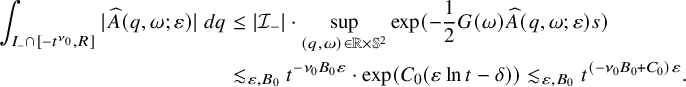 $$ \begin{align*} \int_{I_-\cap[-t^{\nu_0},R]}|\widehat{ A }(q,\omega;\varepsilon)|\ dq&\leq |\mathcal{ I }_-|\cdot\sup_{(q,\omega)\in\mathbb{R}\times\mathbb{S}^2}\exp(-\frac{1}{2}G(\omega)\widehat{ A }(q,\omega;\varepsilon)s)\\ &\lesssim_{\varepsilon,B_0} t^{-\nu_0 B_0\varepsilon}\cdot \exp(C_0(\varepsilon\ln t-\delta))\lesssim_{\varepsilon,B_0} t^{(-\nu_0B_0+C_0)\varepsilon}. \end{align*} $$
The choice of $\nu _0$
implies that
$\nu _0$
implies that $\nu _0B_0>C_0$
, so we have
$\nu _0B_0>C_0$
, so we have $\int _{I_-}|\widehat { A }|\ dq=0$
by sending
$\int _{I_-}|\widehat { A }|\ dq=0$
by sending $t\to \infty $
. Thus, we have
$t\to \infty $
. Thus, we have $\widehat { A }|_{I_-}\equiv 0$
.
$\widehat { A }|_{I_-}\equiv 0$
.
Finally, we show that if $G(\omega )\widehat { A }(q,\omega ;\varepsilon )=0$
everywhere and if
$G(\omega )\widehat { A }(q,\omega ;\varepsilon )=0$
everywhere and if $G(\omega )\not \equiv 0$
on
$G(\omega )\not \equiv 0$
on $\mathbb {S}^2$
, then
$\mathbb {S}^2$
, then $\widehat { A }\equiv 0$
. In fact, in Section 6.2.2, we have mentioned that the set
$\widehat { A }\equiv 0$
. In fact, in Section 6.2.2, we have mentioned that the set $\{\omega \in \mathbb {S}^2:\ G(\omega )=0\}$
has surface measure zero. In other words, we have
$\{\omega \in \mathbb {S}^2:\ G(\omega )=0\}$
has surface measure zero. In other words, we have $\widehat { A }=0$
almost everywhere on
$\widehat { A }=0$
almost everywhere on $\mathbb {S}^2$
. We thus conclude that
$\mathbb {S}^2$
. We thus conclude that $\widehat { A }\equiv 0$
by its continuity.
$\widehat { A }\equiv 0$
by its continuity.
6.2.4 The final step
To end the proof of Proposition 6.2, we show that if $\widehat { A }\equiv 0$
, then
$\widehat { A }\equiv 0$
, then $u\equiv 0$
.
$u\equiv 0$
.
Suppose that $\widehat { A }\equiv 0$
. We first claim that
$\widehat { A }\equiv 0$
. We first claim that $\left \lVert \partial u(t)\right \rVert _{L^2(\mathbb {R}^3)}\lesssim \varepsilon t^{-1/2+C\varepsilon }$
for all
$\left \lVert \partial u(t)\right \rVert _{L^2(\mathbb {R}^3)}\lesssim \varepsilon t^{-1/2+C\varepsilon }$
for all $t\geq 2e^{\delta /\varepsilon }$
. Here, we want to apply Lemma 3.1 instead of (3.14), because Lemma 3.1 holds in the whole region
$t\geq 2e^{\delta /\varepsilon }$
. Here, we want to apply Lemma 3.1 instead of (3.14), because Lemma 3.1 holds in the whole region $\Omega $
. By (3.16), we have
$\Omega $
. By (3.16), we have
 $$ \begin{align*} A(q,\omega)&=\widehat{ A }(F(q,\omega),\omega)=0,\qquad\forall (q,\omega)\in\mathbb{R}\times\mathbb{S}^2. \end{align*} $$
Recall that $A_1A_2=-2A$
and that
$A_1A_2=-2A$
and that $A_1<-1$
. Thus, we also have
$A_1<-1$
. Thus, we also have $A_2\equiv 0$
and thus
$A_2\equiv 0$
and thus $\widetilde { U }\equiv 0$
. Here, we recall the definitions of
$\widetilde { U }\equiv 0$
. Here, we recall the definitions of $A,A_1,A_2,\widetilde { U }$
in (3.5) and (3.6). By Lemma 3.1, we have
$A,A_1,A_2,\widetilde { U }$
in (3.5) and (3.6). By Lemma 3.1, we have
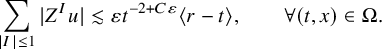 $$ \begin{align*} \sum_{|I|\leq 1}|Z^Iu|\lesssim \varepsilon t^{-2+C\varepsilon}\langle r-t \rangle,\qquad \forall (t,x)\in\Omega. \end{align*} $$
Thus, we have $|\partial u|\lesssim \varepsilon t^{-2+C\varepsilon }$
for all
$|\partial u|\lesssim \varepsilon t^{-2+C\varepsilon }$
for all $(t,x)\in \Omega $
by (2.6). Moreover, whenever
$(t,x)\in \Omega $
by (2.6). Moreover, whenever $t\geq 2e^{\delta /\varepsilon }$
but
$t\geq 2e^{\delta /\varepsilon }$
but $(t,x)\notin \Omega $
, we have
$(t,x)\notin \Omega $
, we have $|x|\leq \frac {1}{2}(t+e^{\delta /\varepsilon })+2R\leq 3t/4+2R\leq 7t/8$
. Since
$|x|\leq \frac {1}{2}(t+e^{\delta /\varepsilon })+2R\leq 3t/4+2R\leq 7t/8$
. Since $Z^Iu=O(\varepsilon t^{-1+C\varepsilon })$
by (3.1), we have
$Z^Iu=O(\varepsilon t^{-1+C\varepsilon })$
by (3.1), we have
 $$ \begin{align*} |\partial u|&\lesssim \langle r-t \rangle^{-1}|Zu|\lesssim t^{-1}\cdot \varepsilon t^{-1+C\varepsilon}\lesssim \varepsilon t^{-2+C\varepsilon},\qquad t\geq 2e^{\delta/\varepsilon},\ (t,x)\not\in\Omega. \end{align*} $$
In summary, we have $|\partial u|\lesssim \varepsilon t^{-2+C\varepsilon }$
for all
$|\partial u|\lesssim \varepsilon t^{-2+C\varepsilon }$
for all $t\geq 2e^{\delta /\varepsilon }$
and all
$t\geq 2e^{\delta /\varepsilon }$
and all $x\in \mathbb {R}^3$
. Since
$x\in \mathbb {R}^3$
. Since $u|_{r-t\geq R}\equiv 0$
, we conclude that
$u|_{r-t\geq R}\equiv 0$
, we conclude that
 $$ \begin{align*} \left\lVert\partial u(t)\right\rVert_{L^2(\mathbb{R}^3)}\lesssim \varepsilon t^{-2+C\varepsilon}\cdot|B(0,t+R)|^{1/2}\lesssim \varepsilon t^{-1/2+C\varepsilon},\qquad \forall t\geq 2e^{\delta/\varepsilon}. \end{align*} $$
This finishes the proof of our claim.
Now, we apply the standard energy estimate from, for example, [Reference Sogge67, Proposition I.2.1]. Since u is a global solution to (1.1), for each $0\leq t_1<t_2$
, we have
$0\leq t_1<t_2$
, we have
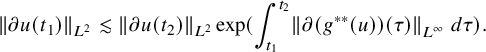 $$ \begin{align}\begin{aligned} \left\lVert\partial u(t_1)\right\rVert_{L^2}\lesssim \left\lVert\partial u(t_2)\right\rVert_{L^2}\exp(\int_{t_1}^{t_2}\left\lVert\partial (g^{**}(u))(\tau)\right\rVert_{L^\infty}\ d\tau). \end{aligned}\end{align} $$
Note that there is no inhomogeneous term in (1.1). Moreover, the energy estimate in [Reference Sogge67, Proposition I.2.1] is forward in time while (6.7) is backward in time. To handle this difference, we simply apply the forward energy estimate to $w(t,x):=u(t_2-t,-x)$
which still solves (1.1).
$w(t,x):=u(t_2-t,-x)$
which still solves (1.1).
By the chain rule and the bound $|\partial u|\lesssim \varepsilon \langle t \rangle ^{-1}$
for all
$|\partial u|\lesssim \varepsilon \langle t \rangle ^{-1}$
for all $t\geq 0$
, we have
$t\geq 0$
, we have
 $$ \begin{align*} \exp(\int_{t_1}^{t_2}\left\lVert\partial (g^{**}(u))(\tau)\right\rVert_{L^\infty}\ d\tau)\lesssim\exp(\int_{t_1}^{t_2}C\varepsilon (1+\tau)^{-1}\ d\tau)\lesssim (\frac{t_2+1}{t_1+1})^{C\varepsilon}. \end{align*} $$
And since $\left \lVert \partial u(t)\right \rVert _{L^2}\lesssim \varepsilon t^{-1/2+C\varepsilon }$
for all
$\left \lVert \partial u(t)\right \rVert _{L^2}\lesssim \varepsilon t^{-1/2+C\varepsilon }$
for all $t\geq 2e^{\delta /\varepsilon }$
, we have
$t\geq 2e^{\delta /\varepsilon }$
, we have
 $$ \begin{align*} \left\lVert\partial u(t)\right\rVert_{L^2}\lesssim \left\lVert\partial u(T)\right\rVert_{L^2}\cdot (\frac{1+T}{1+t})^{C\varepsilon}\lesssim \varepsilon T^{-1/2+C\varepsilon},\qquad \forall 0\leq t\leq T,\ T>2e^{\delta/\varepsilon}. \end{align*} $$
The left side is independent of T. Thus, by choosing $\varepsilon \ll 1$
and sending
$\varepsilon \ll 1$
and sending $T\to \infty $
, we conclude that
$T\to \infty $
, we conclude that $\partial u(t)\equiv 0$
for each
$\partial u(t)\equiv 0$
for each $t\geq 0$
. Since
$t\geq 0$
. Since $u(t,\cdot )$
has a compact support, we have
$u(t,\cdot )$
has a compact support, we have $u\equiv 0$
for all
$u\equiv 0$
for all $(t,x)\in [0,\infty )\times \mathbb {R}^3$
.
$(t,x)\in [0,\infty )\times \mathbb {R}^3$
.
6.3 Corollaries of Proposition 6.2
We finally prove Theorem 3. We will prove a slightly stronger version of this theorem.
Proposition 6.6. Suppose that the quasilinear wave equation (1.1) violates the null condition. Fix $(u_0,u_1)\in C_c^\infty (\mathbb {R}^3)$
and
$(u_0,u_1)\in C_c^\infty (\mathbb {R}^3)$
and $0<\varepsilon \ll 1$
. Let u be the
$0<\varepsilon \ll 1$
. Let u be the $C^\infty $
global solution to (1.1) with initial data
$C^\infty $
global solution to (1.1) with initial data $(\varepsilon u_0,\varepsilon u_1)$
. Also fix
$(\varepsilon u_0,\varepsilon u_1)$
. Also fix $\delta \in (0,1)$
. Then, there exist constants
$\delta \in (0,1)$
. Then, there exist constants $B_0,B_1>0$
depending on
$B_0,B_1>0$
depending on $u_0,u_1,\delta $
(and not on
$u_0,u_1,\delta $
(and not on $\varepsilon $
), such that the following conclusion holds. Suppose that one of the following assumptions holds:
$\varepsilon $
), such that the following conclusion holds. Suppose that one of the following assumptions holds:
-
i) Fix
$0<\nu _0<1$
. For all
$t\geq e^{\delta /\varepsilon }$
and
$\omega \in \mathbb {S}^2$
, we have (6.8)
$$ \begin{align}\begin{aligned} |(u_t-u_r)(t,(t-t^{\nu_0})\omega)|\lesssim \varepsilon t^{-1}\langle t^{\nu_0} \rangle^{-1- B_0\varepsilon}\sim \varepsilon t^{-1-\nu_0-\nu_0B_0\varepsilon}; \end{aligned}\end{align} $$
-
ii) Fix
$0<\nu _0<1$
. For all
$t\geq e^{\delta /\varepsilon }$
and all
$x\in \mathbb {R}^3$
with
$|x|\in [t-2t^{\nu _0},t-t^{\nu _0}/2]$
, we have (6.9)
$$ \begin{align}\begin{aligned} |u(t,x) |\lesssim\varepsilon t^{-1-(\nu_0 B_0+B_1)\varepsilon}; \end{aligned}\end{align} $$
-
iii) Fix
$0<\nu _0<1$
. For all
$t\geq e^{\delta /\varepsilon }$
and
$\omega \in \mathbb {S}^2$
, we have (6.10)Moreover, we have
$$ \begin{align}\begin{aligned} \sum_{1\leq i<j\leq 3}|(\partial_t-\partial_r)\Omega_{ij}u(t,(t-t^{\nu_0})\omega)|\lesssim \varepsilon t^{-1}\langle t^{\nu_0} \rangle^{-1- B_0\varepsilon}\sim \varepsilon t^{-1-\nu_0-\nu_0B_0\varepsilon}. \end{aligned}\end{align} $$
(6.11)
$$ \begin{align}\begin{aligned} |u(t,0)|\lesssim\varepsilon t^{-1-B_0\varepsilon} \qquad \forall t\geq e^{\delta/\varepsilon}. \end{aligned}\end{align} $$


Then, as long as $\varepsilon \ll 1$
which may depend on the constants in each of the assumptions, we have
$\varepsilon \ll 1$
which may depend on the constants in each of the assumptions, we have $u \equiv 0$
.
$u \equiv 0$
.
In its proof, we will apply part c) of Proposition 6.2. Let $C_0>0$
be the constant in part c) of Proposition 6.2. Let the
$C_0>0$
be the constant in part c) of Proposition 6.2. Let the $B_0$
in the statement of Proposition 6.6 be an arbitrary constant larger than
$B_0$
in the statement of Proposition 6.6 be an arbitrary constant larger than $C_0$
(e.g.,
$C_0$
(e.g., $B_0=C_0+1$
). Following Section 3, we obtain a corresponding function
$B_0=C_0+1$
). Following Section 3, we obtain a corresponding function $\widehat { A }$
. It suffices to prove that
$\widehat { A }$
. It suffices to prove that
 $$ \begin{align*} |\widehat{ A }(q,\omega;\varepsilon)|\lesssim_{\varepsilon,B_0} \langle q \rangle^{-1-B_0\varepsilon},\qquad \forall (q,\omega)\in\mathbb{R}\times\mathbb{S}^2. \end{align*} $$
6.3.1 The assumption i)
Lemma 6.7. Fix $0<\nu _0<1$
. Suppose that
$0<\nu _0<1$
. Suppose that
 $$ \begin{align*} |(u_t-u_r)(t,(t-t^{\nu_0})\omega)|\lesssim \varepsilon t^{-1-\nu_0-\nu_0B_0\varepsilon}\langle r(t,\omega)-t \rangle^{-1- B_0\varepsilon},\qquad \forall t\geq e^{\delta/\varepsilon},\ \omega\in\mathbb{S}^2. \end{align*} $$
Then, we have
 $$ \begin{align*} |\widehat{ A }(q,\omega;\varepsilon)|&\lesssim_{B_0,\nu_0}\langle q \rangle^{-1-B_0\varepsilon},\qquad \forall (q,\omega)\in\mathbb{R}\times\mathbb{S}^2. \end{align*} $$
Proof. It is easy to check that $(t,(t-t^{\nu _0})\omega )\in \Omega \cap \{|r-t|\lesssim t^{\nu _0}\}$
whenever
$(t,(t-t^{\nu _0})\omega )\in \Omega \cap \{|r-t|\lesssim t^{\nu _0}\}$
whenever $t\geq e^{\delta /\varepsilon }$
. Thus, by (3.14), we have
$t\geq e^{\delta /\varepsilon }$
. Thus, by (3.14), we have
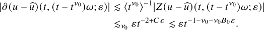 $$ \begin{align*} |\partial (u-\widehat{ u })(t,(t-t^{\nu_0})\omega;\varepsilon)|&\lesssim \langle t^{\nu_0} \rangle^{-1}|Z (u-\widehat{ u })(t,(t-t^{\nu_0})\omega;\varepsilon)|\\ &\lesssim_{\nu_0}\varepsilon t^{-2+C\varepsilon}\lesssim \varepsilon t^{-1-\nu_0-\nu_0B_0\varepsilon}. \end{align*} $$
In the last estimate, we use $-2+C\varepsilon <-1-\nu _0-\nu _0B_0\varepsilon $
as long as
$-2+C\varepsilon <-1-\nu _0-\nu _0B_0\varepsilon $
as long as $\varepsilon \ll _{\nu _0,B_0}1$
. We thus have
$\varepsilon \ll _{\nu _0,B_0}1$
. We thus have
 $$ \begin{align*} |(\partial_t-\partial_r) \widehat{ u } (t,(t-t^{\nu_0})\omega;\varepsilon)|&\lesssim \varepsilon t^{-1-\nu_0-\nu_0B_0\varepsilon}. \end{align*} $$
By (3.24) in Proposition 3.3, we also have
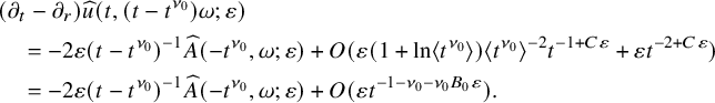 $$ \begin{align*} &(\partial_t-\partial_r) \widehat{ u } (t,(t-t^{\nu_0})\omega;\varepsilon)\\&\quad =-2\varepsilon (t-t^{\nu_0})^{-1}\widehat{ A }(-t^{\nu_0},\omega;\varepsilon)+O(\varepsilon(1+\ln\langle t^{\nu_0} \rangle)\langle t^{\nu_0} \rangle^{-2}t^{-1+C\varepsilon}+\varepsilon t^{-2+C\varepsilon})\\&\quad =-2\varepsilon (t-t^{\nu_0})^{-1}\widehat{ A }(-t^{\nu_0},\omega;\varepsilon)+O(\varepsilon t^{-1-\nu_0-\nu_0B_0\varepsilon}). \end{align*} $$
Previously, we have proved that $\varepsilon t^{-2+C\varepsilon }\lesssim \varepsilon t^{-1}\langle r(t,\omega )-t \rangle ^{-1-B_0\varepsilon }$
. Besides, we have
$\varepsilon t^{-2+C\varepsilon }\lesssim \varepsilon t^{-1}\langle r(t,\omega )-t \rangle ^{-1-B_0\varepsilon }$
. Besides, we have $\varepsilon (1+\ln \langle t^{\nu _0} \rangle )\langle t^{\nu _0} \rangle ^{-2}t^{-1+C\varepsilon }\lesssim _{\nu _0} \varepsilon t^{\nu _0/2-2\nu _0-1+C\varepsilon }\leq \varepsilon t^{-1-\nu _0-\nu _0B_0\varepsilon }$
. In summary, we have
$\varepsilon (1+\ln \langle t^{\nu _0} \rangle )\langle t^{\nu _0} \rangle ^{-2}t^{-1+C\varepsilon }\lesssim _{\nu _0} \varepsilon t^{\nu _0/2-2\nu _0-1+C\varepsilon }\leq \varepsilon t^{-1-\nu _0-\nu _0B_0\varepsilon }$
. In summary, we have
 $$ \begin{align*} |\widehat{ A }(-t^{\nu_0},\omega;\varepsilon)|\lesssim \varepsilon^{-1}(t-t^{\nu_0})\cdot \varepsilon t^{-1-\nu_0-\nu_0B_0\varepsilon}\lesssim \langle t^{\nu_0} \rangle^{-1-B_0\varepsilon}. \end{align*} $$
This estimate holds for all $t\geq e^{\delta /\varepsilon }$
and
$t\geq e^{\delta /\varepsilon }$
and $\omega \in \mathbb {S}^2$
. Thus, we have
$\omega \in \mathbb {S}^2$
. Thus, we have
 $$ \begin{align*} |\widehat{ A }(q,\omega;\varepsilon)|\lesssim \langle q \rangle^{-1-B_0\varepsilon},\qquad \forall q\leq -e^{\nu_0\delta/\varepsilon},\omega\in\mathbb{S}^2. \end{align*} $$
Recall that $\widehat { A }|_{q\leq R}\equiv 0$
. Besides, whenever
$\widehat { A }|_{q\leq R}\equiv 0$
. Besides, whenever $q\in [-e^{\nu _0\delta /\varepsilon },R]$
, we have
$q\in [-e^{\nu _0\delta /\varepsilon },R]$
, we have
 $$ \begin{align*} |\widehat{ A }|\lesssim \langle q \rangle^{-1+C\varepsilon}\lesssim \langle q \rangle^{-1-B_0\varepsilon}\cdot \langle e^{\nu_0\delta/\varepsilon} \rangle^{(B_0+C)\varepsilon}\lesssim_{B_0}\langle q \rangle^{-1-B_0\varepsilon}. \end{align*} $$
This finishes the proof.
6.3.2 The assumption ii)
Assuming (6.9), we will prove that (6.8) holds. Let $B_1>1$
be a constant to be chosen. By taking
$B_1>1$
be a constant to be chosen. By taking $q=-t^{\nu _0}$
and
$q=-t^{\nu _0}$
and $q=-t^{\nu _0}-t^{\nu _0-B_1\varepsilon }$
in (6.9), we obtain
$q=-t^{\nu _0}-t^{\nu _0-B_1\varepsilon }$
in (6.9), we obtain
 $$ \begin{align*} |u(t,(t-t^{\nu_0})\omega)-u(t,(t-t^{\nu_0}-t^{\nu_0-B_1\varepsilon})\omega)|&\lesssim \varepsilon t^{-1-(\nu_0B_0+B_1)\varepsilon}=\varepsilon t^{-1-\nu_0-\nu_0B_0\varepsilon}\cdot t^{\nu_0-B_1\varepsilon}. \end{align*} $$
By the mean value theorem, there exists $b_0\in (0,1)$
such that
$b_0\in (0,1)$
such that
 $$ \begin{align*} |u_r(t,(t-t^{\nu_0}-b_0t^{\nu_0-B_1\varepsilon})\omega)|&\lesssim \varepsilon t^{-1-\nu_0-\nu_0B_0\varepsilon}. \end{align*} $$
Moreover, we notice that
 $$ \begin{align*} |u_{rr}(t,x)|&\lesssim |\partial^2u|+r^{-1}|\partial u|\lesssim \varepsilon t^{-1+C\varepsilon}\langle |x|-t \rangle^{-2},\qquad\forall t\geq 1,\ |x|/t\in[1/2,2]. \end{align*} $$
It follows that
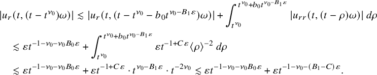 $$ \begin{align*} &|u_r(t,(t-t^{\nu_0})\omega)|\lesssim |u_r(t,(t-t^{\nu_0}-b_0t^{\nu_0-B_1\varepsilon})\omega)|+\int_{t^{\nu_0}}^{t^{\nu_0}+b_0t^{\nu_0-B_1\varepsilon}}|u_{rr}(t,(t-\rho)\omega)|\ d\rho\\&\quad\lesssim \varepsilon t^{-1-\nu_0-\nu_0B_0\varepsilon}+\int_{t^{\nu_0}}^{t^{\nu_0}+b_0t^{\nu_0-B_1\varepsilon}}\varepsilon t^{-1+C\varepsilon}\langle \rho \rangle^{-2}\ d\rho\\&\quad\lesssim \varepsilon t^{-1-\nu_0-\nu_0B_0\varepsilon}+\varepsilon t^{-1+C\varepsilon}\cdot t^{\nu_0-B_1\varepsilon}\cdot t^{-2\nu_0}\lesssim \varepsilon t^{-1-\nu_0-\nu_0B_0\varepsilon}+\varepsilon t^{-1-\nu_0-(B_1-C)\varepsilon}. \end{align*} $$
To estimate the integral in the second row, we notice that $\langle \rho \rangle ^{-2}\sim t^{-2\nu _0}$
. Now, by choosing
$\langle \rho \rangle ^{-2}\sim t^{-2\nu _0}$
. Now, by choosing $B_1$
such that
$B_1$
such that $B_1\geq B_0+C$
, we conclude that
$B_1\geq B_0+C$
, we conclude that $u_r(t,(t-t^{\nu _0})\omega )=O(\varepsilon t^{-1-\nu _0-\nu _0B_0\varepsilon })$
. And since
$u_r(t,(t-t^{\nu _0})\omega )=O(\varepsilon t^{-1-\nu _0-\nu _0B_0\varepsilon })$
. And since $u_t+u_r=O(\varepsilon t^{-2+C\varepsilon })$
, we obtain (6.8).
$u_t+u_r=O(\varepsilon t^{-2+C\varepsilon })$
, we obtain (6.8).
6.3.3 The assumption iii)
Lemma 6.8. Fix $0<\nu _0<1$
. Suppose that
$0<\nu _0<1$
. Suppose that
 $$ \begin{align*} \sum_{1\leq i<j\leq 3}|(\partial_t-\partial_r)\Omega_{ij}u(t,(t-t^{\nu_0})\omega)|\lesssim \varepsilon t^{-1}\langle t^{\nu_0} \rangle^{-1- B_0\varepsilon}\sim \varepsilon t^{-1-\nu_0-\nu_0B_0\varepsilon},\qquad \forall t\geq e^{\delta/\varepsilon},\omega\in\mathbb{S}^2. \end{align*} $$
Then, we have
 $$ \begin{align*} \sum_{1\leq i<j\leq 3}|(\omega_i\partial_{\omega_j}-\omega_j\partial_{\omega_i})\widehat{ A }(q,\omega;\varepsilon)|&\lesssim_{B_0,\nu_0}\langle q \rangle^{-1-B_0\varepsilon},\qquad \forall (q,\omega)\in\mathbb{R}\times\mathbb{S}^2. \end{align*} $$
Proof. By following the proof in Lemma 6.7, we first obtain
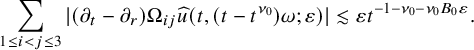 $$ \begin{align*} \sum_{1\leq i<j\leq 3}|(\partial_t-\partial_r) \Omega_{ij} \widehat{ u } (t,(t-t^{\nu_0})\omega;\varepsilon)|&\lesssim \varepsilon t^{-1-\nu_0-\nu_0B_0\varepsilon}. \end{align*} $$
If we chose a multiindex I such that $Z^I=\Omega _{ij}$
, then by (3.26), we have
$Z^I=\Omega _{ij}$
, then by (3.26), we have $A_I=-2(\omega _i\partial _{\omega _j}-\omega _j\partial _{\omega _i})\widehat { A }$
. By (3.24) in Proposition 3.3, we thus have
$A_I=-2(\omega _i\partial _{\omega _j}-\omega _j\partial _{\omega _i})\widehat { A }$
. By (3.24) in Proposition 3.3, we thus have
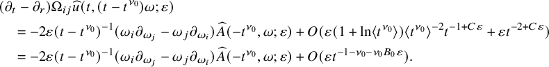 $$ \begin{align*} &(\partial_t-\partial_r) \Omega_{ij} \widehat{ u } (t,(t-t^{\nu_0})\omega;\varepsilon)\\&\quad=-2\varepsilon (t-t^{\nu_0})^{-1}(\omega_i\partial_{\omega_j}-\omega_j\partial_{\omega_i})\widehat{ A }(-t^{\nu_0},\omega;\varepsilon)+O(\varepsilon(1+\ln\langle t^{\nu_0} \rangle)\langle t^{\nu_0} \rangle^{-2}t^{-1+C\varepsilon}+\varepsilon t^{-2+C\varepsilon})\\&\quad=-2\varepsilon (t-t^{\nu_0})^{-1}(\omega_i\partial_{\omega_j}-\omega_j\partial_{\omega_i})\widehat{ A }(-t^{\nu_0},\omega;\varepsilon)+O(\varepsilon t^{-1-\nu_0-\nu_0B_0\varepsilon}). \end{align*} $$
The remaining proof is the same as that of Lemma 6.7.
By (6.11) and (5.4) with $|I|=0$
, we have
$|I|=0$
, we have
 $$ \begin{align*} |\int_{\mathbb{S}^2}\widehat{ A }(-t,\theta;\varepsilon)\ dS_\theta|&\lesssim \varepsilon^{-1}t^{-2+C\varepsilon}+t^{-1-B_0\varepsilon}\lesssim t^{-1-B_0\varepsilon}\qquad \forall t\geq e^{\delta/\varepsilon}. \end{align*} $$
Thus, for all $t\geq e^{\delta /\varepsilon }$
and
$t\geq e^{\delta /\varepsilon }$
and $\omega \in \mathbb {S}^2$
, we have
$\omega \in \mathbb {S}^2$
, we have
 $$ \begin{align*} |\widehat{ A }(-t,\omega;\varepsilon)|&\leq|\widehat{ A }(-t,\omega;\varepsilon)-\frac{1}{4\pi}\int_{\mathbb{S}^2}\widehat{ A }(-t,\theta;\varepsilon)\ dS_\theta|+\frac{1}{4\pi}|\int_{\mathbb{S}^2}\widehat{ A }(-t,\theta;\varepsilon)\ dS_\theta|\\ &\lesssim \int_{\mathbb{S}^2}|\widehat{ A }(-t,\omega;\varepsilon)-\widehat{ A }(-t,\theta;\varepsilon)|\ dS_\theta+t^{-1-B_0\varepsilon}\lesssim_{B_0,\nu_0} t^{-1-B_0\varepsilon}. \end{align*} $$
In the last estimate, we apply Lemma 6.8. It follows that
 $$ \begin{align*} |\widehat{ A }(q,\omega;\varepsilon)|&\lesssim \langle q \rangle^{-1-B_0\varepsilon},\qquad q\leq -e^{\delta/\varepsilon},\omega\in\mathbb{S}^2. \end{align*} $$
Using $\widehat { A }=O(\langle q \rangle ^{-1+C\varepsilon })$
and
$\widehat { A }=O(\langle q \rangle ^{-1+C\varepsilon })$
and $\widehat { A }|_{q\geq R}\equiv 0$
, we can once again prove
$\widehat { A }|_{q\geq R}\equiv 0$
, we can once again prove $|\widehat { A }(q,\omega ;\varepsilon )|\lesssim _{B_0} \langle q \rangle ^{-1-B_0\varepsilon }$
for all
$|\widehat { A }(q,\omega ;\varepsilon )|\lesssim _{B_0} \langle q \rangle ^{-1-B_0\varepsilon }$
for all $(q,\omega )$
.
$(q,\omega )$
.
Acknowledgements
The author would like to thank Sung-Jin Oh and Daniel Tataru for many helpful discussions. The author would also like to thank the anonymous reviewer for valuable comments and suggestions. The author has been funded by a Simons Investigator grant of Daniel Tataru from the Simons Foundation and a VandyGRAF Fellowship from Vanderbilt University.
Competing interest
The author has no competing interests to declare.


 Open access