


1 Introduction
Since the invention of the chirped pulse amplification technique for generating high-power, ultra-short pulses[ Reference Strickland and Mourou 1 ], there has been a rapid development of petawatt class facilities around the world, from one in 1998 to more than 50 in the mid-2010s[ Reference Danson, Hillier, Hopps and Neely 2 ] to several at the 10 PW level and beyond today[ Reference Danson, Haefner, Bromage, Butcher, Chanteloup, Chowdhury, Galvanauskas, Gizzi, Hein, Hillier, Hopps, Kato, Khazanov, Kodama, Korn, Li, Li, Limpert, Ma, Nam, Neely, Papadopoulos, Penman, Qian, Rocca, Shaykin, Siders, Spindloe, Szatmári, Trines, Zhu, Zhu and Zuegel 3 ]. There are multiple limitations to continuing to extend these facilities to ultra-high powers, but one critical technology that has been identified as a challenge[ 4 ] is the pulse compressor, which currently relies on large gratings. Conventional optics have a damage threshold that depends on the coating type and either the fluence or intensity of the incident laser light. In practice, the fluence threshold is at most 1 J/cm2[ Reference Zhang, Kong, Wang, Xing, Zhang, Zhang and Fu 5 ]. Thus, for the 0.1–1 kJ energies required to make petawatt laser pulses, the gratings must be on the square meter scale or larger, which is both a technological and a cost limitation. There is, however, a scientific interest in further increasing the power for studies of, for example, optics in the relativistic regime[ Reference Mourou, Tajima and Bulanov 6 ] to the behavior of matter in extremely strong electromagnetic fields[ Reference Zhang, Bulanov, Seipt, Arefiev and Thomas 7 – Reference Fedotov, Ilderton, Karbstein, King, Seipt, Taya and Torgrimsson 9 ].
One alternative to conventional chirped pulse amplification using a grating compressor is the use of plasma, which has intensity limits for degradation of performance that are many orders of magnitude higher than conventional optical elements. In principle, plasma could be used to compress a chirped pulse through group velocity dispersion, which recently has been theoretically demonstrated for mm-scale, near critical-density plasma[ Reference Hur, Ersfeld, Lee, Kim, Roh, Lee, Song, Kumar, Yoffe, Jaroszynski and Suk 10 ]. At lower plasma densities, however, the required path lengths would be too long for practical use. This motivates the use of a structured plasma that can take advantage of geometric dispersion to compress a pulse over a much smaller spatial footprint.
The use of parametric processes, such as Raman[
Reference Malkin, Shvets and Fisch
11
,
Reference Ping, Cheng, Suckewer, Clark and Fisch
12
] and Brillouin[
Reference Andreev, Riconda, Tikhonchuk and Weber
13
,
Reference Edwards, Jia, Mikhailova and Fisch
14
] scattering, has been explored for amplifiers or for volume compression using plasma Bragg gratings[
Reference Wu, Sheng and Zhang
15
]. These schemes rely on the generation of periodic structures and operation at near-relativistic laser intensities, $I{\lambda}^2\gtrsim {10}^{17}\;\mathrm{W}/{\mathrm{cm}}^2$
, where
$I{\lambda}^2\gtrsim {10}^{17}\;\mathrm{W}/{\mathrm{cm}}^2$
, where $I$
is the intensity and
$I$
is the intensity and $\lambda$
is the wavelength. At such intensities, there are multiple nonlinear processes that can degrade performance, for example, wavebreaking and pre-depletion of the pump laser pulses by thermal plasma[
Reference Farmer, Ersfeld and Jaroszynski
16
], and laser filamentation instabilities[
Reference Kaw, Schmidt and Wilcox
17
]. More recent studies have considered the replacement of the conventional gratings with transient plasma transmission gratings[
Reference Edwards and Michel
18
,
Reference Lehmann and Spatschek
19
]. As transmission gratings require a small amount of plasma and the dispersion comes from geometric considerations, the scheme should be less sensitive to nonlinearities or plasma inhomogeneity. Another method for obtaining the required angular dispersion is through transverse plasma density gradients, which have previously been studied in the context of plasma lenses[
Reference Hubbard, Hafizi, Ting, Kaganovich, Sprangle and Zigler
20
–
Reference Li, Miller, Pierce, Mori, Thomas and Palastro
22
] and for laser steering[
Reference Ma, Cardarelli, Campbell, Fourmaux, Fitzgarrald, Balcazar, Antoine, Beier, Qian, Hussein, Kettle, Klein, Krushelnick, Li, Mangles, Sarri, Seipt, Senthilkumaran, Streeter, Willingale and Thomas
23
,
Reference Ma, Seipt, Dann, Streeter, Palmer, Willingale and Thomas
24
].
$\lambda$
is the wavelength. At such intensities, there are multiple nonlinear processes that can degrade performance, for example, wavebreaking and pre-depletion of the pump laser pulses by thermal plasma[
Reference Farmer, Ersfeld and Jaroszynski
16
], and laser filamentation instabilities[
Reference Kaw, Schmidt and Wilcox
17
]. More recent studies have considered the replacement of the conventional gratings with transient plasma transmission gratings[
Reference Edwards and Michel
18
,
Reference Lehmann and Spatschek
19
]. As transmission gratings require a small amount of plasma and the dispersion comes from geometric considerations, the scheme should be less sensitive to nonlinearities or plasma inhomogeneity. Another method for obtaining the required angular dispersion is through transverse plasma density gradients, which have previously been studied in the context of plasma lenses[
Reference Hubbard, Hafizi, Ting, Kaganovich, Sprangle and Zigler
20
–
Reference Li, Miller, Pierce, Mori, Thomas and Palastro
22
] and for laser steering[
Reference Ma, Cardarelli, Campbell, Fourmaux, Fitzgarrald, Balcazar, Antoine, Beier, Qian, Hussein, Kettle, Klein, Krushelnick, Li, Mangles, Sarri, Seipt, Senthilkumaran, Streeter, Willingale and Thomas
23
,
Reference Ma, Seipt, Dann, Streeter, Palmer, Willingale and Thomas
24
].
In this paper, we present an approach for pulse compression using prisms of uniform underdense plasma that may be made using shaped gas cells, as shown in Figure 1. This design has the advantages of beginning only with gas (and so being reproducible at high repetition rates), using simple geometry, withstanding intensities several orders of magnitude higher than conventional gratings, and remaining relatively compact. With these advantages, plasma-prism compression may offer an approach to plasma-based compression for the next generation of high-power lasers.
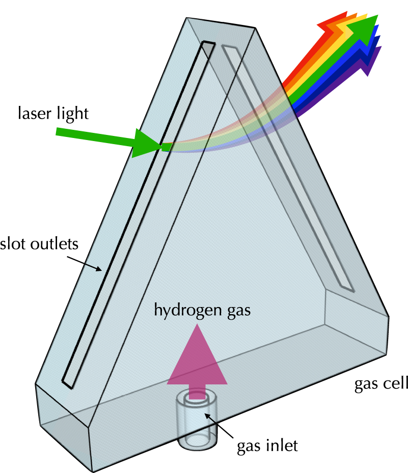
Figure 1 Schematic of a plasma prism based on ionization of hydrogen gas in an additively manufactured gas cell[ Reference Vargas, Schumaker, He, Zhao, Behm, Chvykov, Hou, Krushelnick, Maksimchuk, Yanovsky and Thomas 25 ].
2 Dispersion in plasma
The linear dispersion relation for light propagating in an unmagnetized plasma is ${\omega}^2={c}^2{k}^2+{\omega}_\mathrm{p}^2$
, where
${\omega}^2={c}^2{k}^2+{\omega}_\mathrm{p}^2$
, where ${\omega}_\mathrm{p}=\sqrt{e^2{n}_\mathrm{e}/{m}_\mathrm{e}{\varepsilon}_0}$
is the plasma frequency for electron number density
${\omega}_\mathrm{p}=\sqrt{e^2{n}_\mathrm{e}/{m}_\mathrm{e}{\varepsilon}_0}$
is the plasma frequency for electron number density ${n}_\mathrm{e}$
. The refractive index is therefore
${n}_\mathrm{e}$
. The refractive index is therefore $n\left(\omega \right)=\sqrt{1-{\omega}_\mathrm{p}^2/{\omega}^2}$
. For convenience, we define the relative density of plasma
$n\left(\omega \right)=\sqrt{1-{\omega}_\mathrm{p}^2/{\omega}^2}$
. For convenience, we define the relative density of plasma $N={n}_\mathrm{e}/{n}_\mathrm{c}$
, where
$N={n}_\mathrm{e}/{n}_\mathrm{c}$
, where ${n}_\mathrm{c}={\varepsilon}_0{m}_\mathrm{e}{\omega}_0^2/{e}^2$
is the critical density for the central frequency of the laser,
${n}_\mathrm{c}={\varepsilon}_0{m}_\mathrm{e}{\omega}_0^2/{e}^2$
is the critical density for the central frequency of the laser, ${\omega}_0$
, and
${\omega}_0$
, and ${\varepsilon}_0$
,
${\varepsilon}_0$
, $e$
and
$e$
and ${m}_\mathrm{e}$
are the vacuum permittivity and electron charge and mass, respectively.
${m}_\mathrm{e}$
are the vacuum permittivity and electron charge and mass, respectively.
The temporal profile of a linearly chirped Gaussian pulse can be expressed as follows:
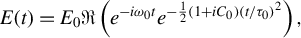 $$\begin{align}E(t)={E}_0\Re \left({e}^{-i{\omega}_0t}{e}^{-\frac{1}{2}\left(1+{iC}_0\right){\left(t/{\tau}_0\right)}^2}\right),\end{align}$$
where ${E}_0$
is the pulse amplitude,
${E}_0$
is the pulse amplitude, ${\tau}_0$
is the half-width at the
${\tau}_0$
is the half-width at the $1/e$
level of intensity and
$1/e$
level of intensity and ${C}_0$
is the linear chirp factor. The bandwidth-limited duration of the pulse is
${C}_0$
is the linear chirp factor. The bandwidth-limited duration of the pulse is ${\tau}_1={\tau}_0/\sqrt{1+{C}_0^2}$
. The frequency bandwidth of the pulse may be quantified by the half-width of
${\tau}_1={\tau}_0/\sqrt{1+{C}_0^2}$
. The frequency bandwidth of the pulse may be quantified by the half-width of ${\left|\widehat{E}\left(\omega \right)\right|}^2$
at the 1/e level,
${\left|\widehat{E}\left(\omega \right)\right|}^2$
at the 1/e level, $\Delta \omega =1/{\tau}_1$
[
Reference Diels and Rudolph
26
].
$\Delta \omega =1/{\tau}_1$
[
Reference Diels and Rudolph
26
].
A frequency component $\omega$
propagating in a dispersive medium will incur a spectral phase
$\omega$
propagating in a dispersive medium will incur a spectral phase $\Psi \left(\omega \right)=\omega P/c$
, where
$\Psi \left(\omega \right)=\omega P/c$
, where $P$
is the optical path length:
$P$
is the optical path length:
 $$\begin{align}P=\int n(\boldsymbol{r})\mathrm{d}r,\end{align}$$
integrated along the frequency-dependent path of propagation. Expanding $\Psi$
in a Taylor series about
$\Psi$
in a Taylor series about ${\omega}_0$
yields
${\omega}_0$
yields
 $$\begin{align}\Psi ={\Psi}_0+\left(\omega -{\omega}_0\right){\Psi}_0^{\prime }+\frac{1}{2}{\left(\omega -{\omega}_0\right)}^2\Psi^{\prime\prime}_0\nonumber\\{}\kern3.24em +\frac{1}{6}{\left(\omega -{\omega}_0\right)}^3\Psi^{\prime \prime \prime}_0+\dots, \end{align}$$
where ${\Psi}_0=\Psi \left({\omega}_0\right)$
and
${\Psi}_0=\Psi \left({\omega}_0\right)$
and ${\left.{\Psi}_0^{\prime}=\mathrm{\partial \Psi }/\partial \omega \right|}_{\omega ={\omega}_0}$
are the phase and group delays, respectively, which only displace the pulse and do not affect the phase fronts or temporal profile. The second-order phase,
${\left.{\Psi}_0^{\prime}=\mathrm{\partial \Psi }/\partial \omega \right|}_{\omega ={\omega}_0}$
are the phase and group delays, respectively, which only displace the pulse and do not affect the phase fronts or temporal profile. The second-order phase,
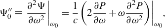 $$\begin{align}\Psi^{\prime\prime}_0\equiv {\left.\frac{\partial^2\Psi}{\partial {\omega}^2}\right|}_{\omega_0}=\frac{1}{c}{\left.\left(2\frac{\partial P}{\partial \omega }+\omega \frac{\partial^2P}{\partial {\omega}^2}\right)\right|}_{\omega_0},\end{align}$$
is the group delay dispersion (GDD) incurred within the medium.
Depending on its sign, the GDD will increase or decrease the linear chirp of a pulse. For instance, the GDD necessary to compress a linearly chirped pulse to the bandwidth limit is $\Psi^{\prime\prime}_0={C}_0{\tau}_0^2/\left(1+{C}_0^2\right)$
[
Reference Diels and Rudolph
26
]. Third-order dispersion (TOD),
$\Psi^{\prime\prime}_0={C}_0{\tau}_0^2/\left(1+{C}_0^2\right)$
[
Reference Diels and Rudolph
26
]. Third-order dispersion (TOD),
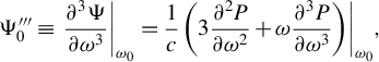 $$\begin{align}\Psi^{\prime\prime\prime}_0\equiv {\left.\frac{\partial^3\Psi}{\partial {\omega}^3}\right|}_{\omega_0}=\frac{1}{c}{\left.\left(3\frac{\partial^2P}{\partial {\omega}^2}+\omega \frac{\partial^3P}{\partial {\omega}^3}\right)\right|}_{\omega_0},\end{align}$$
and higher order terms will distort the Gaussian pulse shape. The spectral phase incurred within an optical system will affect a pulse traveling through it via $\widehat{E}_\mathrm{post}\left(\omega \right)=\widehat{E}_\mathrm{pre}\left(\omega \right){e}^{i\Psi \left(\omega \right)}$
.
$\widehat{E}_\mathrm{post}\left(\omega \right)=\widehat{E}_\mathrm{pre}\left(\omega \right){e}^{i\Psi \left(\omega \right)}$
.
3 Compressor design
The prism compressor is constructed from four plasma prisms. Figure 1 shows a concept for implementation of such a plasma prism in practice, based on additively manufactured gas cells that have been used successfully in laser-wakefield acceleration experiments[
Reference Vargas, Schumaker, He, Zhao, Behm, Chvykov, Hou, Krushelnick, Maksimchuk, Yanovsky and Thomas
25
]. The prisms are arranged symmetrically across a central ‘mirror’ axis, as shown in Figure 2. The apexes of the prisms are spaced a distance $L$
apart, with the second prism apex elevated above the first, forming an angle
$L$
apart, with the second prism apex elevated above the first, forming an angle $\alpha$
. The mirror axis is at a distance
$\alpha$
. The mirror axis is at a distance $M$
from the tip of the second prism. Each prism has a uniform relative plasma density
$M$
from the tip of the second prism. Each prism has a uniform relative plasma density $N<1$
. All frequency components enter the first prism and exit the second prism at the Brewster’s angle
$N<1$
. All frequency components enter the first prism and exit the second prism at the Brewster’s angle ${\theta}_\mathrm{B}=\arctan \left(\sqrt{1-N}\right)$
with respect to the surface. The half-angle of each prism is the Brewster’s angle in plasma
${\theta}_\mathrm{B}=\arctan \left(\sqrt{1-N}\right)$
with respect to the surface. The half-angle of each prism is the Brewster’s angle in plasma ${\theta}_\mathrm{B}^{\prime}=\arctan \left(1/\sqrt{1-N}\right)$
. A ray with frequency
${\theta}_\mathrm{B}^{\prime}=\arctan \left(1/\sqrt{1-N}\right)$
. A ray with frequency $\omega$
enters the second prism at an angle
$\omega$
enters the second prism at an angle ${\varphi}_2$
, which becomes
${\varphi}_2$
, which becomes ${\varphi}_2^{\prime }$
inside the prism. On the other boundary, it exits the plasma at angle
${\varphi}_2^{\prime }$
inside the prism. On the other boundary, it exits the plasma at angle ${\varphi}_1^{\prime }$
, which becomes
${\varphi}_1^{\prime }$
, which becomes ${\theta}_\mathrm{B}$
upon exit to vacuum. These angles can be expressed in terms of the frequency and refractive index of the plasmas as follows:
${\theta}_\mathrm{B}$
upon exit to vacuum. These angles can be expressed in terms of the frequency and refractive index of the plasmas as follows:
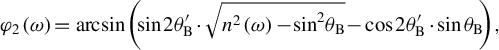 $$\begin{align}{\varphi}_2\left(\omega \right)&{\kern-1pt}={\kern-1pt}\arcsin{\kern-1pt} \left(\!\!\sin 2{\theta}_\mathrm{B}^{\prime}\cdot \sqrt{n^2\left(\omega \right){\kern-1pt}-{\kern-1pt}{\sin}^2{\theta}_\mathrm{B}}{\kern-1pt}-{\kern-1pt}\cos 2{\theta}_\mathrm{B}^{\prime}\cdot \sin {\theta}_\mathrm{B}\!\!\right),\end{align}$$
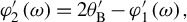 $$\begin{align}{\varphi}_2^{\prime}\left(\omega \right)&=2{\theta}_\mathrm{B}^{\prime }-{\varphi}_1^{\prime}\left(\omega \right),\end{align}$$
 $$\begin{align}{\varphi}_1^{\prime}\left(\omega \right)&=\arcsin \left(\sin {\theta}_\mathrm{B}/n\left(\omega \right)\right).\end{align}$$
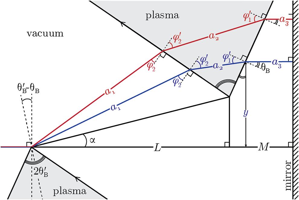
Figure 2 Path of lower frequency (red) and higher frequency (blue) rays through the plasma-prism compressor.
A ray with frequency $\omega$
that travels through the tip of the first prism will travel a length
$\omega$
that travels through the tip of the first prism will travel a length ${a}_1$
between the two prisms,
${a}_1$
between the two prisms, ${a}_2$
within the second prism and
${a}_2$
within the second prism and ${a}_3$
from the second prism to the mirror. Lengths
${a}_3$
from the second prism to the mirror. Lengths ${a}_1,{a}_2\;\mathrm{and}\;{a}_3$
are a function of frequency and are derived from the geometry of the prism arrangement as follows:
${a}_1,{a}_2\;\mathrm{and}\;{a}_3$
are a function of frequency and are derived from the geometry of the prism arrangement as follows:
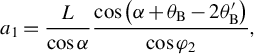 $$\begin{align}{a}_1&=\frac{L}{\cos \alpha}\frac{\cos \left(\alpha +{\theta}_\mathrm{B}-2{\theta}_\mathrm{B}^{\prime}\right)}{\cos {\varphi}_2}, \end{align}$$
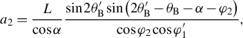 $$\begin{align}{a}_2&=\frac{L}{\cos \alpha}\frac{\sin 2{\theta}_\mathrm{B}^{\prime}\sin \left(2{\theta}_\mathrm{B}^{\prime }-{\theta}_\mathrm{B}-\alpha -{\varphi}_2\right)}{\cos {\varphi}_2\cos {\varphi}_1^{\prime }},\end{align}$$
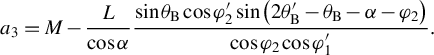 $$\begin{align}{a}_3&=M-\frac{L}{\cos \alpha}\frac{\sin {\theta}_\mathrm{B}\cos {\varphi}_2^{\prime}\sin \left(2{\theta}_\mathrm{B}^{\prime }-{\theta}_\mathrm{B}-\alpha -{\varphi}_2\right)}{\cos {\varphi}_2\cos {\varphi}_1^{\prime }}.\end{align}$$
Assuming sharp vacuum–plasma boundaries, the integration in Equation (2) can be estimated as $P\left(\omega \right)=2\left({a}_1\left(\omega \right)+n\left(\omega \right){a}_2\left(\omega \right)+{a}_3\left(\omega \right)\right)$
. In principle, it is not necessary for the boundaries to be sharp for the concept to work, since for refraction under the ray-tracing approximation, Snell’s law holds for non-sharp. In practice, the additional phase accumulation from boundary ramps could be pre-compensated using a spectral phase control device.
$P\left(\omega \right)=2\left({a}_1\left(\omega \right)+n\left(\omega \right){a}_2\left(\omega \right)+{a}_3\left(\omega \right)\right)$
. In principle, it is not necessary for the boundaries to be sharp for the concept to work, since for refraction under the ray-tracing approximation, Snell’s law holds for non-sharp. In practice, the additional phase accumulation from boundary ramps could be pre-compensated using a spectral phase control device.
The overall spectral phase applied by the compressor is parameterized by $N$
,
$N$
, $L$
and
$L$
and $\alpha$
, that is,
$\alpha$
, that is, $\Psi =\Psi \left(\omega; N,L,\alpha \right)$
. The compressor geometry was optimized using these parameters such that
$\Psi =\Psi \left(\omega; N,L,\alpha \right)$
. The compressor geometry was optimized using these parameters such that $\Psi^{\prime\prime}_0={C}_0{\tau}_0^2/\left(1+{C}_0^2\right)$
and higher order distortions were minimized. To quantify the distorting effect of TOD in particular, the parameter
$\Psi^{\prime\prime}_0={C}_0{\tau}_0^2/\left(1+{C}_0^2\right)$
and higher order distortions were minimized. To quantify the distorting effect of TOD in particular, the parameter $q=\frac{1}{6}\Psi^{\prime\prime\prime}_0\;\Delta {\omega}^3$
is defined as the contribution of TOD to the incurred phase at
$q=\frac{1}{6}\Psi^{\prime\prime\prime}_0\;\Delta {\omega}^3$
is defined as the contribution of TOD to the incurred phase at $\omega ={\omega}_0+\Delta \omega$
. Figure 3 shows the parameter phase space of
$\omega ={\omega}_0+\Delta \omega$
. Figure 3 shows the parameter phase space of $L$
and
$L$
and $\alpha$
such that
$\alpha$
such that $\Psi^{\prime\prime}_0=10,000$
(e.g., designed to compress a pulse with
$\Psi^{\prime\prime}_0=10,000$
(e.g., designed to compress a pulse with ${\tau}_0=1000$
fs,
${\tau}_0=1000$
fs, ${C}_0=100$
to
${C}_0=100$
to ${\tau}_1=10$
fs) for normalized densities
${\tau}_1=10$
fs) for normalized densities $N$
varying from 0.1 to 0.005 and assuming sharp plasma boundaries. The angle
$N$
varying from 0.1 to 0.005 and assuming sharp plasma boundaries. The angle $\alpha$
is defined to be negative when the apex of the second prism is below the first, and is limited above by the angle of refraction of the highest frequency in the pulse and limited below by the first prism. Thus,
$\alpha$
is defined to be negative when the apex of the second prism is below the first, and is limited above by the angle of refraction of the highest frequency in the pulse and limited below by the first prism. Thus, $\alpha$
is constrained by
$\alpha$
is constrained by ${\Psi}_0^{\prime\prime}\left({\omega}_\mathrm{max}\right)<2{\theta}_\mathrm{B}^{\prime }-{\theta}_\mathrm{B}-\alpha <\pi /2$
, where
${\Psi}_0^{\prime\prime}\left({\omega}_\mathrm{max}\right)<2{\theta}_\mathrm{B}^{\prime }-{\theta}_\mathrm{B}-\alpha <\pi /2$
, where ${\omega}_\mathrm{max}$
can be approximated as
${\omega}_\mathrm{max}$
can be approximated as ${\omega}_0+2\Delta \omega$
. Larger densities and more negative values
${\omega}_0+2\Delta \omega$
. Larger densities and more negative values $\alpha$
apply the necessary GDD in less distance. While the initial linear chirp is eliminated from the pulse, TOD is significant in this region of parameter space. Using Equations (9)–(11) and (5), we calculate
$\alpha$
apply the necessary GDD in less distance. While the initial linear chirp is eliminated from the pulse, TOD is significant in this region of parameter space. Using Equations (9)–(11) and (5), we calculate $q$
along each line plotted in Figure 3 and plot it in Figure 4. Here,
$q$
along each line plotted in Figure 3 and plot it in Figure 4. Here, $q$
decreases with decreasing
$q$
decreases with decreasing $N$
and decreasing
$N$
and decreasing $\alpha$
, but always remains
$\alpha$
, but always remains $q>2$
. The criterion for minimal shape distortion is
$q>2$
. The criterion for minimal shape distortion is $q\ll 0.1$
, which is not possible by optimizing parameters
$q\ll 0.1$
, which is not possible by optimizing parameters $N$
,
$N$
, $L$
and
$L$
and $\alpha$
alone.
$\alpha$
alone.
Figure 3 Allowed values of $L$
and
$L$
and $\alpha$
such that
$\alpha$
such that $\Psi^{\prime\prime}_0=10,000$
for densities
$\Psi^{\prime\prime}_0=10,000$
for densities $N$
varying from 0.1 to 0.005 (colored lines, labeled).
$N$
varying from 0.1 to 0.005 (colored lines, labeled).

Figure 4 Third-order distortion $q$
for densities
$q$
for densities $N$
varying from 0.1 to 0.005 such that
$N$
varying from 0.1 to 0.005 such that $\Psi^{\prime\prime}_0=10,000$
, showing that TOD needs to be compensated for.
$\Psi^{\prime\prime}_0=10,000$
, showing that TOD needs to be compensated for.
Figure 5 shows the shape distorting effects of TOD on a bandwidth-limited pulse. When $q$
is 0, the pulse is near transform-limited. As
$q$
is 0, the pulse is near transform-limited. As $q$
increases, the peak intensity drops, and additional peaks appear earlier in time.
$q$
increases, the peak intensity drops, and additional peaks appear earlier in time.
Figure 5 Effects of TOD on a bandwidth-limited pulse showing that $q>2$
corresponds to a severe TOD phase error.
$q>2$
corresponds to a severe TOD phase error.
To correct TOD errors, the spectral phase of the uncompressed pulse may be pre-compensated in the front end of the laser chain. Alternatively, a correcting plasma slab with a polynomial density profile can be inserted at the mirror axis. This is the plane where the frequency components of the incoming pulse are spatially dispersed, vertically.
Halfway through the compressor, a ray with frequency $\omega$
is located a distance
$\omega$
is located a distance $y$
above the first prism:
$y$
above the first prism:
 $$\begin{align}y\left(\omega \right){\kern-1pt}={\kern-1pt}\frac{L}{\cos \alpha}\left(\!\sin \alpha +\frac{\cos {\theta}_\mathrm{B}\cos {\varphi}_2^{\prime}\sin \left(2{\theta}_\mathrm{B}^{\prime }{\kern-1pt}-{\kern-1pt}{\theta}_\mathrm{B}{\kern-1pt}-{\kern-1pt}\alpha {\kern-1pt}-{\kern-1pt}{\varphi}_2\right)}{\cos {\varphi}_1^{\prime}\cos {\varphi}_2}\!\right),\end{align}$$
which to first order in frequency is $y\left(\omega \right)={y}_0+A\left(\omega -{\omega}_0\right)$
. Define a rectangular slab of plasma centered horizontally at the mirror axis with width
$y\left(\omega \right)={y}_0+A\left(\omega -{\omega}_0\right)$
. Define a rectangular slab of plasma centered horizontally at the mirror axis with width $W$
and relative density profile
$W$
and relative density profile $N\left(y\left(\omega \right)\right)={N}_0+B{\left(y-{y}_0\right)}^3$
. The spectral phase accumulated over a length
$N\left(y\left(\omega \right)\right)={N}_0+B{\left(y-{y}_0\right)}^3$
. The spectral phase accumulated over a length $W$
is
$W$
is
 $$\begin{align}\Psi \left(\omega \right)=\frac{\omega }{c} Wn\left(\omega \right)=\frac{\omega }{c}W\sqrt{1-\frac{N\left(\omega \right){\omega}_0^2}{\omega^2}},\end{align}$$
for which the GDD is
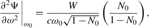 $$\begin{align}{\left.\frac{\partial^2\Psi}{\partial {\omega}^2}\right|}_{\omega_0}=\frac{W}{c{\omega}_0\sqrt{1-{N}_0}}\left(\frac{N_0}{1-{N}_0}\right),\end{align}$$
and the TOD is
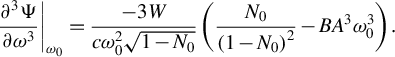 $$\begin{align}{\left.\frac{\partial^3\Psi}{\partial {\omega}^3}\right|}_{\omega_0}=\frac{-3W}{c{\omega}_0^2\sqrt{1-{N}_0}}\left(\frac{N_0}{{\left(1-{N}_0\right)}^2}-{BA}^3{\omega}_0^3\right).\end{align}$$
From Equations (5) and (15), it follows that $B$
must equal
$B$
must equal
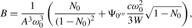 $$\begin{align}B=\frac{1}{A^3{\omega}_0^3}\left(\frac{N_0}{{\left(1-{N}_0\right)}^2}+{\Psi}_{{{0^{\prime\prime\prime}}}}\frac{c{\omega}_0^2}{3W}\sqrt{1-{N}_0}\right),\end{align}$$
and the correcting slab will compensate for the TOD incurred by the other four prisms.
4 Simulation in OSIRIS
The full plasma-prism compressor, including TOD compensation, was simulated in two dimensions with the particle-in-cell (PIC) framework OSIRIS[ Reference Fonseca, Silva, Tsung, Decyk, Lu, Ren, Mori, Deng, Lee, Katsouleas and Adam 27 , Reference Davidson, Tableman, An, Tsung, Lu, Vieira, Fonseca, Silva and Mori 28 ]. OSIRIS solves Faraday and Ampere’s laws in differential form using the finite difference time domain technique. By solving these equations, OSIRIS captures effects that cannot be modeled with ray tracing, such as the finite pulse width and duration and nonlinear plasma dynamics.
The laser pulse is initialized with a Gaussian temporal and transverse profile with $1/e$
intensity duration
$1/e$
intensity duration $\tau$
and width
$\tau$
and width ${w}_0$
. The simulation window moves in the
${w}_0$
. The simulation window moves in the $x$
direction at the speed of light and is of size (4000
$x$
direction at the speed of light and is of size (4000 $c/{\omega}_0)\ \times$
(4500
$c/{\omega}_0)\ \times$
(4500 $c/{\omega}_0)= 509\;\mu \mathrm{m}\times 573\;\mu \mathrm{m}$
and had
$c/{\omega}_0)= 509\;\mu \mathrm{m}\times 573\;\mu \mathrm{m}$
and had $8192\times 8192=6.7\times {10}^7$
grid points. The time step used was
$8192\times 8192=6.7\times {10}^7$
grid points. The time step used was $\Delta t=0.395/{\omega}_0=0.168$
fs. Each simulation cell contained two electrons, for a total of
$\Delta t=0.395/{\omega}_0=0.168$
fs. Each simulation cell contained two electrons, for a total of $1.3\times {10}^8$
particles. For a pulse wavelength of
$1.3\times {10}^8$
particles. For a pulse wavelength of $0.8\;\mu \mathrm{m}$
, the (angular) frequency is
$0.8\;\mu \mathrm{m}$
, the (angular) frequency is ${\omega}_0=2.355\;{\mathrm{fs}}^{-1}$
. The laser pulse started with length
${\omega}_0=2.355\;{\mathrm{fs}}^{-1}$
. The laser pulse started with length ${\tau}_0=100$
fs, chirp factor
${\tau}_0=100$
fs, chirp factor ${{C}_0=10}$
, amplitude
${{C}_0=10}$
, amplitude ${a}_0=0.05$
and spot size
${a}_0=0.05$
and spot size ${w}_0=12.84\;\mu \mathrm{m}$
, corresponding to a Rayleigh length of
${w}_0=12.84\;\mu \mathrm{m}$
, corresponding to a Rayleigh length of ${z}_\mathrm{R}=647\;\mu \mathrm{m}$
. Here,
${z}_\mathrm{R}=647\;\mu \mathrm{m}$
. Here, ${{a}_0={eE}_0/\left({m}_\mathrm{e}c{\omega}_0\right)}$
is the normalized vector potential amplitude of the laser electric field. The pulse was polarized in the
${{a}_0={eE}_0/\left({m}_\mathrm{e}c{\omega}_0\right)}$
is the normalized vector potential amplitude of the laser electric field. The pulse was polarized in the $x$
–
$x$
– $y$
plane. The prism system had relative plasma density
$y$
plane. The prism system had relative plasma density $N=0.2$
, distance between apexes
$N=0.2$
, distance between apexes $L=800\kern0.24em \mu \mathrm{m}$
and angle
$L=800\kern0.24em \mu \mathrm{m}$
and angle $\alpha =-8{}^{\circ}$
. The correction slab had width
$\alpha =-8{}^{\circ}$
. The correction slab had width $W=100\;\mu \mathrm{m}$
, central relative density
$W=100\;\mu \mathrm{m}$
, central relative density ${N}_0$
= 0.03 and density growth factor
${N}_0$
= 0.03 and density growth factor ${B=1.512\times {10}^{-7}\;{\mu \mathrm{m}}^{-3}}$
.
${B=1.512\times {10}^{-7}\;{\mu \mathrm{m}}^{-3}}$
.
Figure 6 shows the intensity profile of the pulse overlaid on the prism compressor at seven locations along its trajectory. Simulation outputs are plotted roughly every 1.8 ps. The pulse can be seen compressing in duration as it travels from left to right through the system. The system is symmetric about the mirror axis at $x=1350\;\mu \mathrm{m}$
. The dashed lines show the results of ray tracing through the compressor for frequencies
$x=1350\;\mu \mathrm{m}$
. The dashed lines show the results of ray tracing through the compressor for frequencies ${\omega}_0\pm 2\Delta \omega$
, calculated by applying Snell’s law at each boundary and propagating to the next boundary. The simulated pulse remains confined by these paths for roughly three Rayleigh lengths before the effects of diffraction can be observed in the transverse spreading of the pulse. This spreading could be mitigated by beginning with a larger spot size
${\omega}_0\pm 2\Delta \omega$
, calculated by applying Snell’s law at each boundary and propagating to the next boundary. The simulated pulse remains confined by these paths for roughly three Rayleigh lengths before the effects of diffraction can be observed in the transverse spreading of the pulse. This spreading could be mitigated by beginning with a larger spot size ${w}_0\ge 2\sqrt{c\left(L+M\right)/{\omega}_0}$
, such that the length of the system is no more than one Rayleigh length.
${w}_0\ge 2\sqrt{c\left(L+M\right)/{\omega}_0}$
, such that the length of the system is no more than one Rayleigh length.
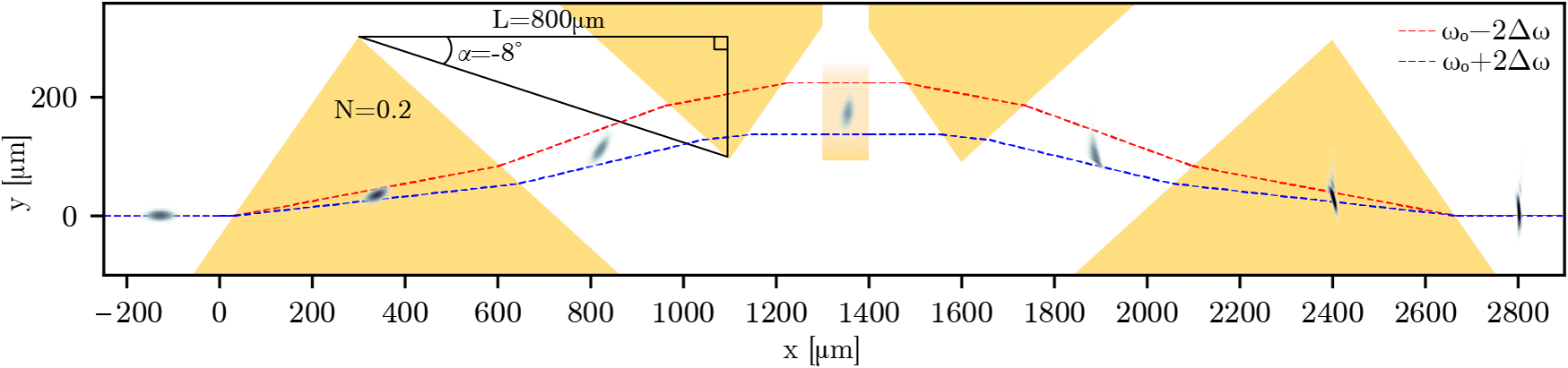
Figure 6 Full compression of a pulse with duration ${\tau}_0=100$
fs is simulated in OSIRIS using a plasma-prism system. The plasma density profile is plotted in yellow. Seven simulation outputs are plotted with timestamps. The dashed lines show the expected paths of
${\tau}_0=100$
fs is simulated in OSIRIS using a plasma-prism system. The plasma density profile is plotted in yellow. Seven simulation outputs are plotted with timestamps. The dashed lines show the expected paths of ${\omega}_0\pm 2\Delta \omega$
frequency components.
${\omega}_0\pm 2\Delta \omega$
frequency components.
Figure 7 compares the initial and final pulse profiles with the transform-limited profile and theoretically predicted profile. The simulated pulse ends with a full width at half-maximum (FWHM) of 22.4 fs, a compression ratio of 7.4 from its initial duration of 166.5 fs and 1.3 times the transform-limited duration of 16.6 fs. The simulated profile has a 20% narrower FWHM and longer tails than the analytical profile, likely due to wavefront curvature that the theory cannot account for. Both have a peak power of 83 GW.
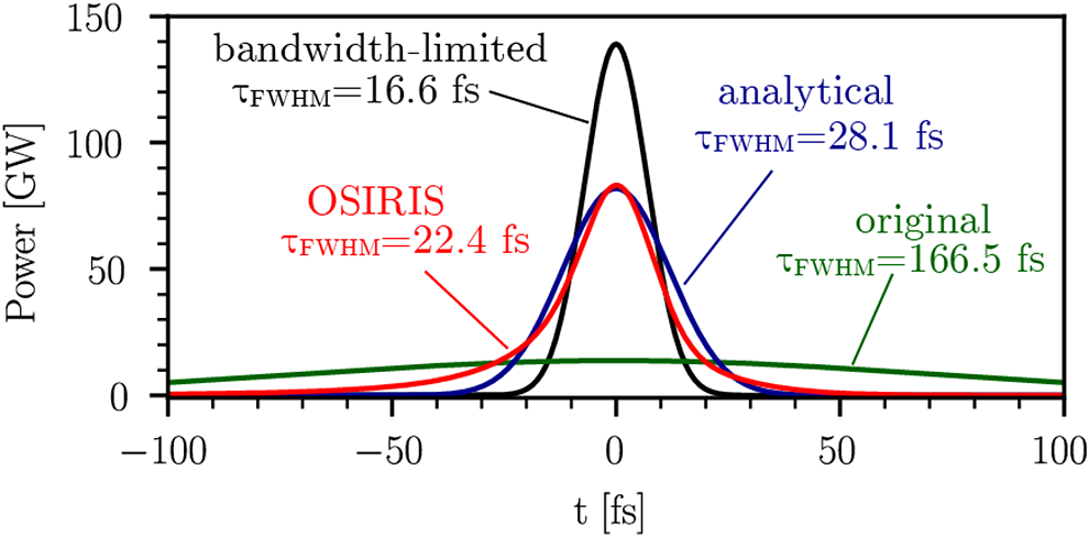
Figure 7 Comparison of initial, simulated, analytical and transform-limited pulse power profiles.
5 Discussion
The OSIRIS simulation confirms the feasibility of femtosecond pulse compression using plasma prisms. Estimating the resulting pulse shape given a particular compressor geometry with the analytically derived expressions can be completed near instantly, whereas the OSIRIS simulation ran in parallel for roughly 12 hours on 36 cores. The compressor used a relatively high density of $N=0.2$
to shrink the system to less than 3 mm in length to reduce computation time. There are other effects that need to be accounted for to improve the accuracy of this analytical estimation, including diffraction, wavefront curvature and more realistic density profiles at the prism–vacuum interfaces. However, it should be noted that, having been successfully demonstrated by direct ab initio simulation at high density/compact size, scaling up to higher powers with larger focal spots, where the Rayleigh length is longer, would be even more accurately described by ray tracing.
$N=0.2$
to shrink the system to less than 3 mm in length to reduce computation time. There are other effects that need to be accounted for to improve the accuracy of this analytical estimation, including diffraction, wavefront curvature and more realistic density profiles at the prism–vacuum interfaces. However, it should be noted that, having been successfully demonstrated by direct ab initio simulation at high density/compact size, scaling up to higher powers with larger focal spots, where the Rayleigh length is longer, would be even more accurately described by ray tracing.
The compression of a pulse is sensitive to the exact GDD incurred. The simulation geometry applies a GDD of $864\;{\mathrm{fs}}^2$
, 13.6% less than
$864\;{\mathrm{fs}}^2$
, 13.6% less than $1000\;{\mathrm{fs}}^2$
necessary to achieve the transform limit. The resulting pulse is 35% longer and has 38% less power than if it were transform-limited. The system geometry could be further optimized to compress pulses closer to the bandwidth limit.
$1000\;{\mathrm{fs}}^2$
necessary to achieve the transform limit. The resulting pulse is 35% longer and has 38% less power than if it were transform-limited. The system geometry could be further optimized to compress pulses closer to the bandwidth limit.
Additional OSIRIS simulations (not shown) indicate that the trajectory of the pulse remains largely unaffected when the sharp plasma boundaries are replaced by $200\;\mu \mathrm{m}$
ramps. However, the GDD is sensitive to the presence of the ramp (because of the added optical path). To incorporate this into the analytical expressions one would need to trace the frequency-dependent trajectory in a density gradient and integrate the optical path length in Equation (2). Step-function boundaries were assumed in the derivation of Equations (9)–(11) so that closed-form expressions for the partial derivatives in Equations (4) and (5) would exist.
$200\;\mu \mathrm{m}$
ramps. However, the GDD is sensitive to the presence of the ramp (because of the added optical path). To incorporate this into the analytical expressions one would need to trace the frequency-dependent trajectory in a density gradient and integrate the optical path length in Equation (2). Step-function boundaries were assumed in the derivation of Equations (9)–(11) so that closed-form expressions for the partial derivatives in Equations (4) and (5) would exist.
In the case of femtosecond pulses, the damage threshold for conventional diffraction gratings is of the order of ${10}^{13}$
–
${10}^{13}$
– ${10}^{14}$
W/cm2[
Reference Gamaly, Rode, Luther-Davies and Tikhonchuk
29
,
Reference Stuart, Feit, Herman, Rubenchik, Shore and Perry
30
]. The peak intensity of the simulated pulse reached
${10}^{14}$
W/cm2[
Reference Gamaly, Rode, Luther-Davies and Tikhonchuk
29
,
Reference Stuart, Feit, Herman, Rubenchik, Shore and Perry
30
]. The peak intensity of the simulated pulse reached $1.14\times {10}^{16}$
W/cm2. At this intensity, no nonlinear phenomena that could disrupt the compression process were observed. Although the simulated pulse power reached 83 GW, self-focusing was not observed. The critical power for self-focusing is
$1.14\times {10}^{16}$
W/cm2. At this intensity, no nonlinear phenomena that could disrupt the compression process were observed. Although the simulated pulse power reached 83 GW, self-focusing was not observed. The critical power for self-focusing is ${P}_\mathrm{cr}\approx \left(17/N\right)$
GW[
Reference Sun, Ott, Lee and Guzdar
31
], which for the parameters here means that
${P}_\mathrm{cr}\approx \left(17/N\right)$
GW[
Reference Sun, Ott, Lee and Guzdar
31
], which for the parameters here means that $P/{P}_\mathrm{cr}\sim 1$
. Even for higher powers, however, previous studies have shown that self-focusing may not occur for ultra-short pulses even if the pulse peak power is many times larger than the critical power[
Reference Faure, Malka, Marquès, David, Amiranoff, Phuoc and Rousse
32
,
Reference Polynkin and Kolesik
33
].
$P/{P}_\mathrm{cr}\sim 1$
. Even for higher powers, however, previous studies have shown that self-focusing may not occur for ultra-short pulses even if the pulse peak power is many times larger than the critical power[
Reference Faure, Malka, Marquès, David, Amiranoff, Phuoc and Rousse
32
,
Reference Polynkin and Kolesik
33
].
The fastest growing parametric instability that can disrupt the compression would be stimulated Raman scattering (SRS). A positive chirp in ultra-short pulses in underdense plasma has been found to increase backward SRS[
Reference Deng, Yue, Luo, Zhao, Li, Ge, Liu, Weng, Chen, Yuan and Zhang
34
,
Reference Dodd and Umstadter
35
]. Limiting backward SRS by constraining ${\gamma}_0{\tau}_\mathrm{FWHM}<12$
, where
${\gamma}_0{\tau}_\mathrm{FWHM}<12$
, where ${\gamma}_0=\left(1/2\right){a}_0{\omega}_0\sqrt{\left({\omega}_\mathrm{p}/{\omega}_0\right)/\left(1-{\omega}_\mathrm{p}/{\omega}_0\right)}$
is the SRS growth rate[
Reference Wilks, Kruer, Williams, Amendt and Eder
36
], imposes an upper bound on the peak laser intensity and optimal system geometry. In terms of the prism density
${\gamma}_0=\left(1/2\right){a}_0{\omega}_0\sqrt{\left({\omega}_\mathrm{p}/{\omega}_0\right)/\left(1-{\omega}_\mathrm{p}/{\omega}_0\right)}$
is the SRS growth rate[
Reference Wilks, Kruer, Williams, Amendt and Eder
36
], imposes an upper bound on the peak laser intensity and optimal system geometry. In terms of the prism density $N$
, this constraint can be expressed as
$N$
, this constraint can be expressed as $N<1/{\left(1+\left(\ln 2/144\right){\left({\omega}_0{a}_0{\tau}_0\right)}^2\right)}^2$
. For the simulated parameters
$N<1/{\left(1+\left(\ln 2/144\right){\left({\omega}_0{a}_0{\tau}_0\right)}^2\right)}^2$
. For the simulated parameters $N=0.2$
is less than
$N=0.2$
is less than ${N}_\mathrm{SRS}=0.36$
, which is consistent with the absence of SRS in the simulations.
${N}_\mathrm{SRS}=0.36$
, which is consistent with the absence of SRS in the simulations.
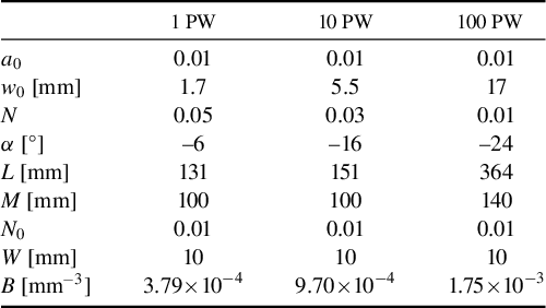
Given the constraints on beam spot size and prism density, Table 1 lists theoretical design parameters that could be used for compact high-power systems that incur a GDD of $1000\;{\mathrm{fs}}^2$
, such as for compressing a
$1000\;{\mathrm{fs}}^2$
, such as for compressing a ${\tau}_0=1$
ps,
${\tau}_0=1$
ps, ${C}_0=100$
pulse to
${C}_0=100$
pulse to ${\tau}_1=10$
fs. The total system size for these compressors is on the scale of 1 m. Note that in practice, the gas would require ionization. For hydrogen gas the barrier suppression ionization (BSI) intensity is of the order of
${\tau}_1=10$
fs. The total system size for these compressors is on the scale of 1 m. Note that in practice, the gas would require ionization. For hydrogen gas the barrier suppression ionization (BSI) intensity is of the order of ${10}^{14}$
W/cm2, which is two orders of magnitude below the peak intensity, and so the gas may be considered to be fully ionized far before the main pulse peak intensity. However, the initial 1 ps long chirped pulse would be close to the BSI intensity and may therefore require some system for (pre-)ionizing the plasma along the laser path, for example, ionization by a second laser, electrical discharge or cylindrically focusing in the
${10}^{14}$
W/cm2, which is two orders of magnitude below the peak intensity, and so the gas may be considered to be fully ionized far before the main pulse peak intensity. However, the initial 1 ps long chirped pulse would be close to the BSI intensity and may therefore require some system for (pre-)ionizing the plasma along the laser path, for example, ionization by a second laser, electrical discharge or cylindrically focusing in the $z$
direction to result in higher intensity in the earlier prisms.
$z$
direction to result in higher intensity in the earlier prisms.
Table 1 Proposed design parameters for higher power compressors that supply a GDD of $1000\;{\mathrm{fs}}^2$
.
$1000\;{\mathrm{fs}}^2$
.
Ionization of the plasma will be an important consideration for an experimental demonstration. It should also be noted that the studies here only considered collisionless ideal plasma, but it is clear that thermal corrections, fluctuations, collisional effects, etc., will affect the dispersive properties of the plasma prisms and potentially laser energy absorption. For random fluctuations, however, the resulting phase errors may be expected to average to zero over long scales. The effects of ionization and neutral gas as well as non-sharp plasma–vacuum boundaries may generate non-zero averaging phase errors that may need compensation. Proof-of-principle experiments and detailed calculations investigating these effects are left for further work.
6 Conclusions
A novel compressor for high-power femtosecond pulses based on underdense plasma prisms can operate at intensities that are orders of magnitude higher than systems using diffraction gratings or solid-state prisms. An analytical model was developed to calculate the spectral phase acquired in the compressor and the corresponding pulse compression. The theory was verified with OSIRIS PIC simulations. Using only plasma prisms, it is impossible to completely eliminate TOD through geometric optimization. However, the TOD could be compensated in the laser front end or by introducing a plasma slab with a cubic density profile at the center of the compressor. Within these constraints, a compact high-power compressor with overall dimensions of less than 1 m can be designed. At the intensities simulated (10 ${}^{16}$
W/cm2), neither self-focusing nor SRS was observed.
${}^{16}$
W/cm2), neither self-focusing nor SRS was observed.
Acknowledgements
This work was supported by US NSF awards 2108075 and 2126181. The work of JPP was supported by the Office of Fusion Energy Sciences under Award No. DE-SC0021057, the Department of Energy National Nuclear Security Administration under Award No. DE-NA0004144 and the New York State Energy Research and Development Authority. This research was supported in part through computational resources and services provided by Advanced Research Computing at the University of Michigan, Ann Arbor.


 Open access