

1 Introduction
The equation of state (EOS) of carbon at high pressures (megabar or multimegabar regime) is of interest for several branches of physics.
In material science, carbon is a unique element owing to its polymorphism, the complexity and variety of its state phases, including graphite, graphene, diamond, etc. Diamond is one of the hardest known materials with a bulk modulus of 4.42 Mbar. The EOS of carbon at high pressures has been the subject of several important experimental and theoretical scientific works.
Many initial theoretical works from the 1970s and early 1980s analyzed the characteristics of carbon at high pressure, including predictions for the heat of fusion, melting point, transformation of graphite to diamond, and metallization of carbon[1–5]. Later theoretical works (1987–1999), often based on numerical simulations using ab initio calculations, resulted in establishing a full picture for the phase diagram of carbon[6–9]. More recently, accurate first-principle multiphase EOSs for carbon at high pressures and temperatures have been established[10–13].
Experimental results were initially obtained using diamond anvil cells. These have demonstrated pressures up to 4 Mbar[14–16]. In this case, the study was also motivated by understanding the behavior of diamond as the tool used in the anvil cell to compress other sample materials to high pressures.
Initial shock experiments were conducted in the early 1980s and provided evidence that the carbon diamond melting line has a positive slope in the P-T diagram[Reference Shaner, Brown, Swenson and McQueen17]. Recent experiments have been performed using laser-driven shocks[18–20], to explore higher pressures, or laser-heated diamond anvils[Reference Benedetti, Nguyen, Caldwell, Liu, Kruger and Jeanloz21, Reference Cavalleri, Sokolowski-Tinten, von der Linde, Spagnolatti, Bernasconi, Benedek, Podestá and Milani22]. Several laser-shock experiments have also been performed to investigate the behavior of high-density carbon (HDC) as a possible ablator to be used in implosion experiments related to inertial confinement fusion[Reference Nellis, Hamilton, Holmes, Radousky, Ree, Mitchell and Nicol23, Reference Ness, Acuña, Behannon, Burlaga, Connerney, Lepping and Neubauer24].
Despite all these works, the behavior of carbon at very high pressures is not yet fully understood. The important phenomenon of carbon metallization[Reference Grover2, Reference Bundy25] at high pressure has long been predicted theoretically but until now never clearly observed in experiments.
In astrophysics, the description of high-pressure phases is essential for developing realistic models of planets and stars[26–28]. Carbon is a major constituent (through methane and carbon dioxide) of giant planets such as Uranus and Neptune and white dwarf stars, but also of many recently discovered extra solar planets (e.g., Gliese 436 b[Reference Butler, Vogt, Marcy, Fischer, Wright, Henry, Laughlin and Lissauer29], which is a ‘hot’ Neptune, or PSR J1719-1438b orbiting a pulsar, which might be substantially carbon-enriched[Reference Bailes, Bates, Bhalerao, Bhat, Burgay, Burke-Spolaor, D'Amico, Johnston, Keith, Kramer, Kulkarni, Levin, Lyne, Milia, Possenti, Spitler, Stappers and van Straten30]).
High pressures are thought to produce methane pyrolysis with a separation of the carbon phase and the possible formation of a diamond or metallic layer[31–34]. Metallization of the carbon layer in the mantle of these planets (the ‘ice layers’) could give a high electrical conductivity and, by the dynamo effect, be the source of the observed large magnetic fields[Reference Ness, Burlaga, Connerney, Lepping and Neubauer35, Reference Connerney, Acuña and Ness36].
The effect of carbon structure in astrophysics was first pointed out by Ross in a now-famous article on ‘diamonds in the sky’ in 1981[Reference Guillot27]. As shown in Ref. [Reference Eggert, Hicks, Celliers, Bradley, McWilliams, Jeanloz, Miller, Boehly and Collins37], the issue is still open, and ‘even if it is now accepted that the high-pressure, high-temperature behavior of carbon is essential to predicting the evolution and structure of such planets, still, one of the most defining of thermal properties for diamond, the melting temperature, has never been directly measured’ (quote from [Reference Nellis, Holmes, Mitchell, Hamilton and Nicol33]). Here, it is worth noting that recently diamond formation was shown at planetary conditions produced by laser shocks[Reference Kraus, Vorberger, Pak, Hartley, Fletcher, Frydrych, Galtier, Gamboa, Gericke, Glenzer, Granados, MacDonald, MacKinnon, McBride, Nam, Neumayer, Roth, Saunders, Schuster, Sun, van Driel, Döppner and Falcone38].
In this context, we performed an experiment to study the behavior of carbon at pressures up to 9 Mbar. We used the PHELIX laser facility at GSI Darmstadt to irradiate multilayered diamond targets to induce laser-driven shock compression producing high-pressure and high-temperature states. Our measurements show that for the pressures obtained in diamond, the propagation of the shock induces a reflecting state of the material. Shock dynamics was modeled using the Lagrangian-hydrodynamic, one-dimensional code MULTI[Reference Ramis, Schmalz and Meyer-Ter-Vehn39] accounting for radiation transfer. We used different EOSs for carbon, showing that our results are compatible with the SESAME tables developed for diamond (and not with other EOSs of carbon).
2 Experimental setup
The experiment was performed at GSI facility using the PHELIX laser, a flash lamp-pumped Nd:glass laser frequency doubled to a wavelength λ = 527 nm. The temporal profile was Gaussian with a duration of 1 ns full width at half maximum (FWHM) and the spatial profile was flat-top with spot ∼500 μm FWHM obtained by an appropriate phase plate[Reference Koenig, Faral, Boudenne, Batani, Benuzzi and Bossi40]. The laser was focused on multilayered targets (plastic/nickel/diamond/nickel) producing a maximum on-target intensity I ∼ 8 × 10¹³–9 × 10¹³ W/cm2. This intensity allows ablation pressures of approximately 12 Mbar to be generated in our plastic ablator (parylene with gross chemical formula C8H8), as can be estimated for instance using well-known scaling-laws[Reference Lindl41]
 $$\begin{align}P =8.6 (I/10^{14})^{2/3}\lambda^{-2/3}{(A/2Z)}^{1/3},\end{align}$$
where A and Z are the atomic mass number and atomic number of the target material; I is in W/cm2, P in Mbar, and  $\lambda\ \text{in}\ \mu\text{m}$. The shock pressure is then increased in nickel due to impedance mismatch[Reference Batani, Balducci, Nazarov, Lφwer, Koenig, Faral, Benuzzi and Temporal42], and decrease again when the shock is transmitted to diamond. This is shown in detail by hydrodynamics simulations (as described in Section 5).
A schematic and an optical photo of diamond target used in this experiment are shown in Figure 1. Polished synthetic single crystal (SC) type-IIa chemical vapor deposition (CVD) (100)-oriented diamond substrates (3 mm × 3 mm in size) were used as target. These substrates were produced by Soni Tools and Soni CVD Diamonds. Typical thicknesses were in the range of 200–300 μm.

Figure 1 (a) Scheme of the target used in the experiment and (b) image of Ni layer deposited on target rear side (taken before deposition of the Ni layer on the target front side).
Nickel layers of about 20 μm in thickness were deposited both on the front side and on half of the rear side (see Figure 1) by means of a metallic stencil at the Institute for Microelectronics and Microsystems (IMM) of CNR. In particular, 1 μm thick Ni films were first deposited on diamond surfaces by a radiofrequency (RF) sputtering technique in diode configuration, using a commercial MRC 8620 system equipped with a cryogenic vacuum pump. The background pressure of the system is lower than 10–7 Torr. The sputtering conditions were as follows: RF power 350 W, target 6″ Ni (purity 99.999%), substrates to target distance 5 cm, Ar flow rate 90 sccm, total pressure 3 mTorr, and substrate temperature 260°C.
It is worth pointing out that although nickel is not a standard EOS reference (e.g., like Al) in high-pressure physics, it was chosen in this experiment because of its better adhesion performance on diamond surface. After that, the pure Ni thick layer (about 19 μm in thickness) was made by electroplating deposition by using a standard manual galvanic growth system (nickel plating solution at 55°C, current density 100 A/m2).
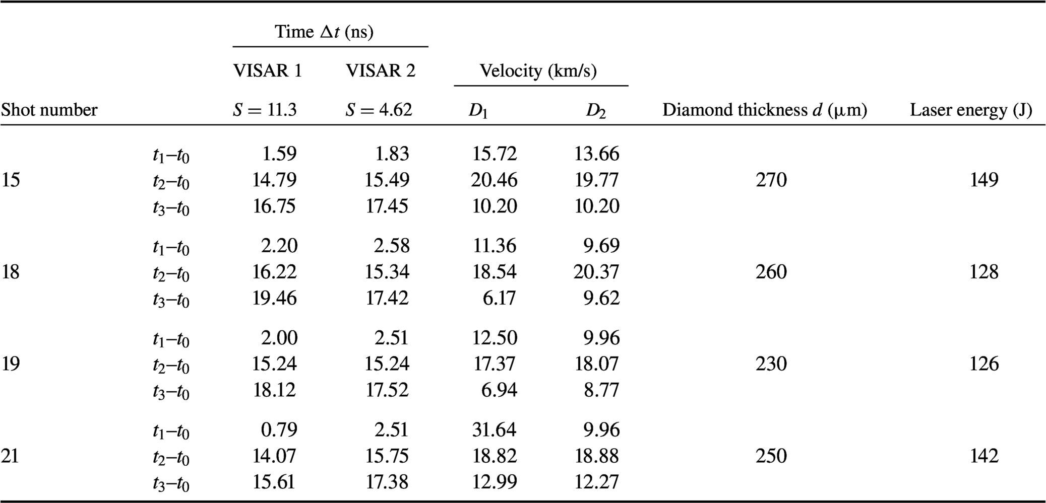
Finally, on some targets, 5 μm of plastic (parylene C8H8 with density ρ = 1.1 g/cm3) was deposited on the target front side to act as a low-Z ablator. The detailed characteristics of the targets can be found in Table 1 for the four useful laser shots obtained in the experiment (from a total of 10 laser shots).
Table 1 Obtained experimental results using shock chronometry. We report the thickness of the diamond layer, the laser energy, the shock breakout times from VISAR data, and the corresponding shock velocities. For the first layer, the shock velocity is just an average value obtained by dividing the total 25 μm thickness (plastic ablator + first nickel layer) by the shock breakout time.
Owing to the low Z of the ablator, X-ray emission is low and characterized by low photon energy. Such X-rays are completely stopped in the Ni layer, so that preheating of diamond is negligible in our experiment. The Ni layer also acts as reflecting surface for the laser probe beam, used for the VISAR diagnostics.
This target design allows the shock breakout at the Ni/diamond, diamond/vacuum, and Ni/vacuum interfaces to be detected, thereby allowing average shock velocities in diamond and nickel to be determined. In addition, the evolution of shock dynamics can be continuously followed in diamond by looking at the VISAR fringe shift. Finally, after shock breakout, we can measure the Ni and diamond free surface velocities by looking again at the VISAR fringe shift.
As diagnostics we used a VISAR. This is a standard diagnostic allowing the velocity of a reflecting surface to be measured through the Doppler effect[43–45]. The main components of the VISAR diagnostic are a seeded probe laser with λ0 = 660 nm and two Mach–Zehnder interferometers. The probe beam is reflected back from the target, and an imaging system creates an image of the target rear side on the output beam splitter in the interferometer. Finally, this is imaged on the slit of a streak camera to provide temporal resolution. A linear fringe pattern is formed owing to the interference of the two beams going through the two interferometer arms with a different delay. The streak camera provides a continuous measurement of shock evolution for several nanoseconds with temporal resolution of the order of ±300 ps.
An optical element (etalon) is added to one of the arms of the interferometer to provide the optical delay while maintaining the spatial coherence between the two arms. The thickness of the etalon fixes the sensitivity of the VISAR. The velocity is measured from the fringe shift. The sensitivity S of the VISAR is measured in km/(s·fringe) and given by
 $$\begin{align}S=\frac{\lambda_0}{2{\tau}_0\left(1+\delta \right)},\end{align}$$
where τ0 is determined by the etalon thickness and δ ∼ 0.03 is determined by the optical dispersion of the etalon glass.
The relation among fringe shift, the sensitivity, and the velocity depends on the environment around the reflecting surface. Basically, there are two cases.
The first case is when the pressure is strong enough to induce a phase transition to a reflecting state, it is directly the shock front travelling in the material that reflects the probe beam. In this case, the velocity of the shock front is measured as
 $$\begin{align}D= SF/{n}_0.\end{align}$$
Here F = ΔΦ/2π is the fringe shift and n 0 is the refractive index of the crossed material (in our case diamond and n 0 = 2.417). This formula also applies to the case of the reflection from a free surface moving in vacuum and in this case of course n 0 = 1. This is indeed what happens after shock breakout at the target rear side when the whole target begins to move.
The second case corresponds to weaker shocks that compress the material but do not induce a reflecting phase, so that it remains transparent. In this case, the probe beam can be reflected from another material behind the transparent one. The interface moves at a velocity U that corresponds to the fluid velocity of the transparent material behind the shock front. The different cases are shown in Figure 2.

Figure 2 Reflection of the VISAR probe beam: (a) from a reflecting shock traveling in the material; (b) from a free surface travelling in vacuum; (c) from a reflecting surface embedded in a compressed transparent material.
In the second case, the beam is reflected from the interface but the velocity U is not measured directly because the fringe shift also depends on the thickness of the compressed material between the interface and the shock front. The relation is in this case given by
 $$\begin{align}D{n}_0-n\left(D-U\right)= SF,\end{align}$$
where n is the refractive index of the compressed material. We see that U cannot be extracted directly. However, if both D and U are known, or measured, this formula allows measuring the refractive index of the compressed material. This approach has been used in Refs. [Reference Batani, Jakubowska, Benuzzi-Mounaix, Cavazzoni, Danson, Hall, Kimpel, Neely, Pasley, Rabec Le Gloahec and Telaro46, Reference Jakubowska, Batani, Clerouin and Siberchicot47] to measure the refractive index of water in the megabar pressure range.
However, if we use the Gladstone–Dale law to describe the refractive index,
 $$\begin{align}n-1=\kappa \rho,\end{align}$$
where  $\kappa$ is a proportionality constant and ρ is the density of the compressed material, after some algebra we arrive at the formula
 $$\begin{align}U= SF\Bigg/\left[1+\left(n-1\right)\frac{\rho }{\rho_0}\frac{\delta }{\delta +1}\right].\end{align}$$
Again, this is not an explicit formula because the measurement of U depends on the degree of compression, i.e., on the ratio of the density of the compressed material to its initial density ρ0. In practical cases, however, physical insight or results from numerical simulations can suggest an appropriate value for ρ/ρ0 so that Equation (6) can be used to obtain a ‘reasonable’ value of U.
Finally, the standard approach used in laser-driven shock experiments is to use two VISARs, i.e., two interferometers with different sensitivity S (given by different etalons). This is related to the intrinsic ambiguity in the VISAR measurements as a result of the 2π periodicity in the fringe interference: using two VISARs allows the ambiguity in fringe jumps to be reduced.
From the VISAR raw data we can extract the phase shift using a Fourier transform algorithm[Reference Takeda, Ina and Kobayashi48].
3 Experimental results: shock chronometry
In this section, we start the presentation of the shots obtained in our experiments and listed in Table 1. Figure 3 shows typical experimental results. These refer to shot 15 as reported in Table 1.

Figure 3 VISAR streak camera images from shot 15: (a) VISAR with sensitivity S = 11.3 km/(s·fringe); (b) VISAR with sensitivity S = 4.62 km/(s·fringe). The total time windows are 32.98 ns for VISAR1 and 30.47 ns for VISAR2. Images were recorded on a 16-bit CCD with 1280 × 1024 pixels giving a conversion of ∼30 ps/pixel.
In Figure 3, we can clearly identify the passage of the shock from one material and the other by the changes in reflectivity and the fringe jumps. These images allow shock chronometry to be performed and because the thickness of the various layers is known, to infer the average shock velocity in each material.
For instance, in Figure 3 the gray dashed line corresponds to the shock breakout at the nickel/diamond interface (t 1), the red dashed line to the shock breakout at the diamond/vacuum interface (t 2), the bottom orange dashed line to the shock breakout at the nickel/vacuum interface (t 3). Finally, the upper green dashed line corresponds to the arrival (of the maximum) of the main laser pulse on target front side (t 0). This is obtained from the time fiducial: the short signal on the right of Figure 3(a) and on the left of Figure 3(b). Such a time fiducial is obtained by sending a small part of the laser pulse onto the streak camera slit by using an optical fiber. The time interval between such time fiducial and the arrival of the maximum of the main laser pulse on target front side is obtained thanks to a calibration shot that is performed without target (i.e., the main laser pulse is directly sent to the streak, after attenuation, together with the time fiducial).
From this we can directly obtain the shock transit times in the plastic/nickel, diamond, and rear-side nickel layers, and then we can obtain the average shock velocity in each layer, as reported in Table 1. The times (and the velocities) obtained from the two VISARs are in fair agreement once the experimental error bars are taken into account. The time resolution of ±300 ps for the shock breakout at two interfaces, together with a maximum (estimated) error in measurement of the thickness of less than ±0.5 μm, gives a typical error on shock velocity measured in diamond of
 $$\begin{align}\frac{\Delta D}{D}\approx \sqrt{2{\left(\frac{0.3\ \mathrm{ns}}{14\ \mathrm{ns}}\right)}^2+{\left(\frac{0.5\ \mu \mathrm{m}}{250\ \mu \mathrm{m}}\right)}^2}\approx 0.03.\end{align}$$
In addition, from the measured average shock velocities, we can obtain an evaluation of the pressure reached in diamond by considering the Hugoniot curve of this material, according to which a shock velocity of ∼20 km/s corresponds to a shock pressure of ∼5.5 Mbar[49].
Our experimental data reflect the expected trends, that is, the shock breakout time decreases when the laser energy increases or when the target thickness decreases. For instance, by comparing shots 18 and 21 (which have almost the same thickness) we see that when the energy increases, the shock breakout at the diamond vacuum interface (t 2) decreases. Similarly, by comparing shots 15 and 21, which have almost the same energy, we see that decreasing the target thickness implies a decrease of shock breakout time.
4 Experimental results: fringe shifts
Unfortunately, in our experiment the fringe quality is poor, which makes it difficult to use the fringe shift for a very precise determination of velocities. In our images, we can confidently evaluate a fringe shift of 1/3 of the wavelength which, with a sensitivity of 4.62 km/(s·fringe) gives an incertitude in shock velocity of ΔD ∼ 1.5 km/s.
Nevertheless, the images are usable and we can retrieve the velocities of reflecting surfaces. To extract velocities from the fringe shift, we used the software NEUTRINO developed by Vinci and Flacco[Reference Flacco and Vinci50]. This software also allows to remove the so-called ghost fringes, i.e., the fringes that arise because of spurious reflections (e.g., from the rear side window of the target or from optics in the pathway).
The basic question to be asked is what we are seeing in VISAR images, i.e., is the probe beam reflected from a reflecting shock front or rather diamond remains transparent and is it reflected by the nickel layer behind the shock? In the first case, we should use Equation (3) with the value of the refractive index of diamond (n 0 = 2.417). In the second case we should use Equation (6), which allows the fluid velocity of the nickel interface U to be retrieved only if the value of ρ/ρ 0 is known. The hydrodynamics simulations presented in Section 5 shows that the shock is not stationary and that the compression degree changes from an initial ρ/ρ 0 ∼ 1.7 when the shock enters in diamond, to a final ρ/ρ 0 ∼ 1.3 when the shock breaks out at the diamond rear side. This would correspond, using the Gladstone–Dale law, to refractive indexes of compressed diamond of 2.84 and 3.41, respectively. Such values seem to be a bit larger than what can be extrapolated from the recent experimental measurements by Ozaki et al.[Reference Katagiri, Ozaki, Miyanishi, Kamimura, Umeda, Sano, Sekine and Kodama51] who reported n ∼ 2.55 at ρ ∼ 4.4 g/cm3 (i.e., a compression ρ/ρ 0 ∼ 1.25) but the change is not very important for the discussion that follows. Calculating the denominator in Equation (6) we see that the initial value is ∼1.248 and the final value is ∼1.206. We see that the variation is not large, and hence we can use an average value of the denominator ∼1.23 in Equation (6) to deduce U from fringe shift F with a reasonable accuracy.
Thus, first we tested the possibility that the probe beam is reflected from the nickel interface by using Equation (6) as just described. In this case, we cannot retrieve an initial value of the fluid velocity, which is in agreement with the available Hugoniot curves for diamond (this would give U ∼ 8–10 km/s, for a shock velocity D ∼ 20 km/s). In addition, at later time, as is clearly shown by the simulations in the next section, the interface velocity U strongly decreases, whereas the VISARs provide an almost constant velocity (as implied by the almost straight vertical fringes in Figure 3).
Therefore, we can conclude that the observed fringes must be produced by a reflection of the probe beam on the shock front. In this case, Figure 4 shows the variation of shock velocity with time obtained from simultaneously analyzing the fringe shifts from the two VISARs. As we can see, the value of shock velocity is in fair agreement with what we have found from shock chronometry (see Table 1) and the measured velocity is almost constant, again as implied by the almost straight vertical fringes in Figure 2. In fact, Figure 4 shows a small decay of velocity with time, i.e., the shock wave as it travels in diamond, in agreement with our expectations (see next section). However, such reduction is not easily measurable owing to the low fringe quality in our experiment.

Figure 4 Time history of the shock velocity in diamond obtained by analyzing the fringe shift of the two VISARs from shot 15 (Figure 3). Here t = 0 is the time of shock breakout at the inner nickel/diamond interface and the shock breakout at diamond rear side takes place 13.48 ns afterwards. The first part of the graph represents the shock velocity in diamond. The second part shows the free surface velocity of diamond after shock breakout at the target rear side.
Finally, after the shock breakout at the rear of the target, we still see a fringe shift. From this, we can calculate the velocity at which the rear-side surface is moving. This is called ‘free surface velocity’ V FS and can be obtained by extrapolating the impedance mismatch conditions to zero pressure and density (in this case we used n 0 = 1, the refractive index of vacuum, to calculate the speed). In the case of ‘weak’ shocks, such free surface is related to the fluid velocity U (the velocity of matter behind the shock front) by the relation V FS ∼2U (see Ref. [Reference Zel'dovich and Raizer52]). From the analysis of the fringe shifts from the two VISARs, we obtained the free surface velocities of diamond and nickel that are reported in Table 2.
Table 2 Comparison of experimental and numerical results for shot 15. Simulations were performed using the SESAME table 7830.

Notes: aaverage of two VISARs; bjust after shock breakout.
5 Hydro simulations
To interpret our experimental results, we performed 1D radiative hydrodynamic simulations with the code MULTI[Reference Ness, Burlaga, Connerney, Lepping and Neubauer35].
The laser pulse was flat top in time with a plateau duration of 1 ns and rise and fall times of 0.1 ns. In the simulations, we used the SESAME table 3100 for nickel and the SESAME table 7770 for parylene[Reference Celliers, Bradley, Collins, Hicks, Boehly and Armstrong45]. As for diamond, we tested different EOS tables coming from the SESAME database[Reference Celliers, Bradley, Collins, Hicks, Boehly and Armstrong45], from QEOS[Reference More, Warren, Young and Zimmerman53] and FEOS[Reference Faik, Tauschwitz and Iosilevskiy54], in all cases setting the initial density at ρ0 = 3.515 g/cm3.
Figure 5 shows the density map and the pressure map from MULTI 1D simulation reproducing shot 15. Here we used the SESAME table 7830 for diamond. Table 2 reports the detailed numerical comparison between experimental and numerical results for shot 15, whereas Table 3 summarizes the main results for all our four useful shots.
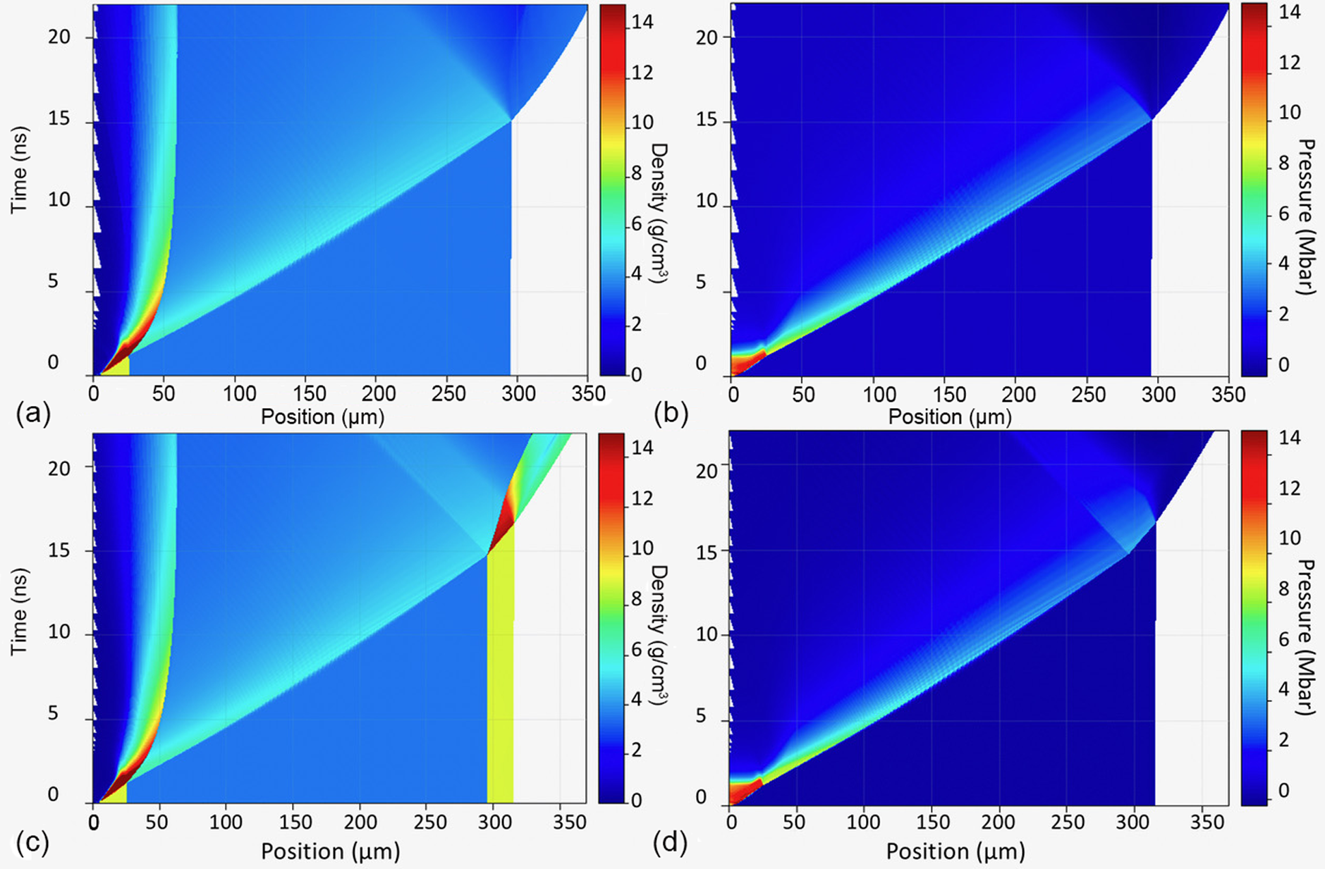
Figure 5 (a) Density map of hydrodynamic simulations from MULTI 1D reproducing shot 15. (b) Pressure map of the same shot. (c), (d) Hydrodynamic simulations with the Ni step. Such plots allow the free surface velocity to be estimated for the Ni step and the diamond layer, respectively.
Table 3 Comparison of experimental and numerical results for all shots (note that the laser intensity reported in this table is the intensity used in hydro simulations in order to reproduce experimental data).

Notes: aaverage of two VISARs; bat the time of shock breakout at the first nickel/diamond interface.
As stated previously, the typical ablation pressure in plastics is ∼12 Mbar for this shot (for which I = 9 × 10¹³ W/cm2), in agreement with the previous scaling law, and this increases in nickel due to the impedance mismatch up to a maximum pressure of ∼26 Mbar as can also be seen using the analytical formulas reported in Ref. [Reference Kraus, Vorberger, Pak, Hartley, Fletcher, Frydrych, Galtier, Gamboa, Gericke, Glenzer, Granados, MacDonald, MacKinnon, McBride, Nam, Neumayer, Roth, Saunders, Schuster, Sun, van Driel, Döppner and Falcone38] for the shock passage between two materials (labelled 1 and 2):
 $$\begin{align}\frac{P_2}{P_1}=\frac{4{\rho}_2}{{\left(\sqrt{\rho_1}+\sqrt{\rho_2}\right)}^2}.\end{align}$$
Before reaching the nickel/diamond interface the pressure in nickel decreases down to ∼15 Mbar. Indeed, as the shock is transmitted from plastic to nickel, a reflected shock with the same pressure (∼26 Mbar) is reflected back into plastic. As soon as this shock reaches the ablation surface (where the pressure applied by the laser is still ∼12 Mbar), a rarefaction wave is generated and quickly reaches the shock front decreasing its pressure.
At this point, the pressure generated in diamond is ∼9 Mbar, again in agreement with Equation (8). Later the shock in diamond decreases down to ≤4 Mbar at the time of shock breakout at the diamond rear side. Although the pressure is nonconstant, the variation in shock velocity is limited (as shown by both experimental results and simulations). This is due to the square root dependence of shock velocity on pressure which implies that the ratio of final shock velocity to initial shock velocity is at most ∼(4/9)1/2 = 0.67. Indeed, the simulation shows a decrease of instantaneous shock velocity in diamond from the initial value ∼24 km/s to a final value of at shock breakout ∼18 km/s (i.e., a ratio of ∼0.75). By comparison, the graph in Figure 4 only shows a decrease of shock velocity from ∼24 km/s down to ∼22 km/s.
At this point, we must justify the use of 1D simulations in order to interpret our experimental results. The 1D approximation is justified because the focal spot (∼500 μm) is large compared with the total target thickness (∼300 μm). However, this is only a qualitative criterion. In reality, the justification of the 1D approximation comes from two experimental results.
(i) The VISAR images (see Figure 3) show that the shock breakout is quite flat both at the nickel/diamond interface and at the target rear side. Now it is well known that 2D effects will produce a curvature at the shock front, initially affecting the edges of the shock front, but gradually progressing to the center. The absence of observable curvature in our images suggests indeed that 2D effects in hydrodynamics are negligible.
(ii) As we have just discussed, the velocity of the shock in our case is decaying quite slowly and actually (within error bars) the decay is compatible with results of 1D simulations (or even seems to be a bit smaller). Now the decrease of shock pressure and shock velocity during propagation is due to two phenomena: (a) the relaxation wave from target front side catching up the travelling shock and (b) bidimensional effects in shock front propagation. The fact that the simulations are in fair agreement with experiment considering only the phenomenon (a) is indeed a proof that (b) is not important. If this was the case, we would expect a much faster decay of shock pressure and velocity.
Finally, to be absolutely certain of the validity of the 1D approximation, we also performed 2D simulations, and compared results with 1D simulations. As the goal here was just to show that 2D effects can be neglected, we did not simulate the full targets with three layers, but we just considered a diamond target of 300 μm thickness and in both 1D and 2D simulations we used the same EOS (SESAME table 7830). The laser was flat top in space and time with spot diameter 500 μm, duration 1 ns at 0.53 μm, and intensity 9 × 10¹³ W/cm2.
The 1D simulation shows a shock breakout at the diamond rear side of 14.2–14.3 ns. The results of 2D simulations (for pressure) at the time 14.3 ns are shown in Figure 6. As you can see the time of the shock arrival to the rear side is perfectly reproduced in 2D simulations, and the shock can be considered as a planar shock at least up to a distance of ≤100 μm from the laser spot center.
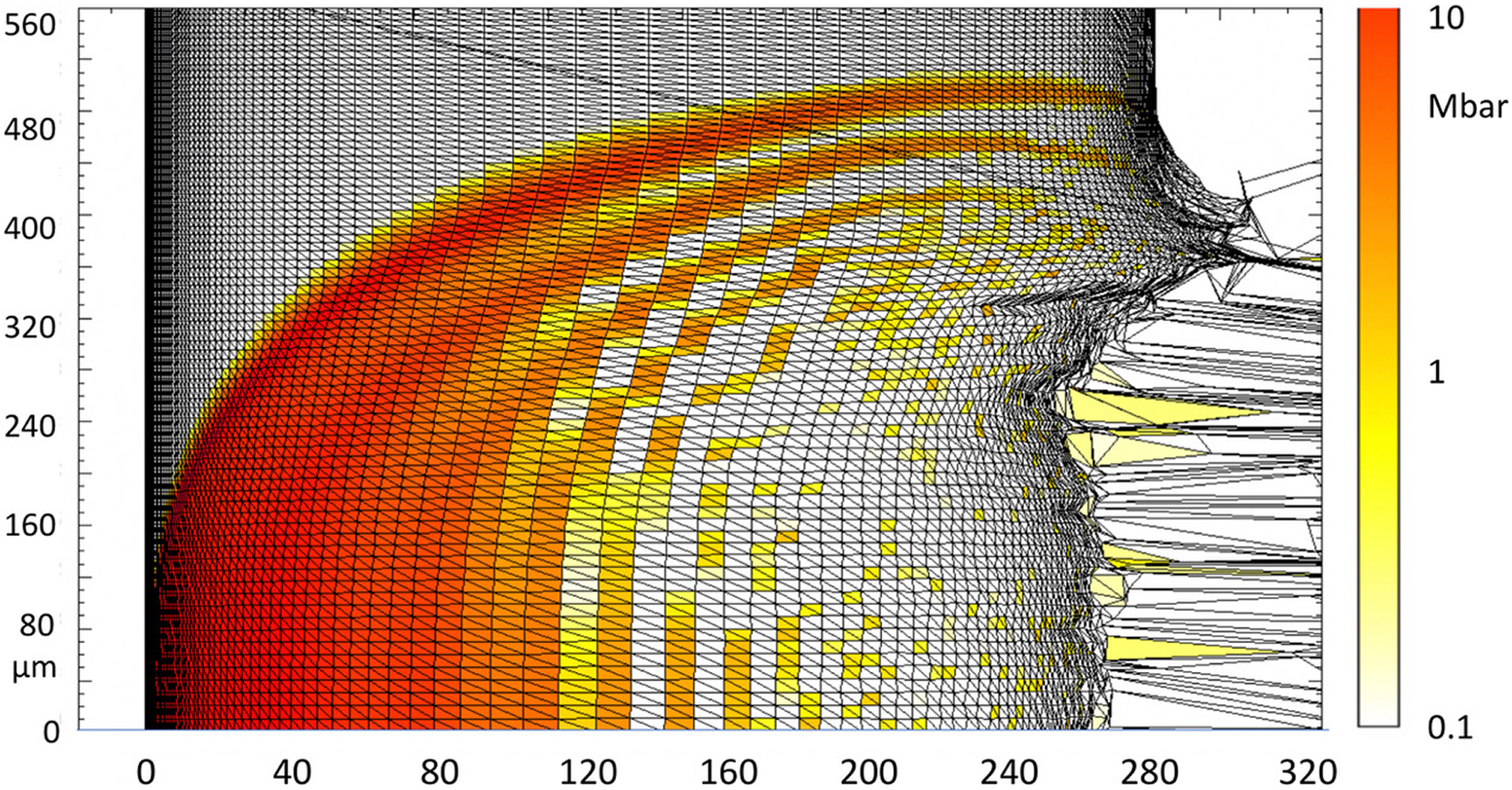
Figure 6 Result of MULTI 2D simulation. Pressure map (in cgs units) at 14.3 ns within a 300 μm thick target irradiated by a 0.53 μm laser, flat top in space (spot diameter 500 μm) and time (duration 1 ns) with intensity 9 × 10¹³ W/cm2.
Returning to Figure 5, we performed two sets of simulations, with and without the final Ni layer, corresponding to what takes place in the two halves of the target. The importance of performing such separate simulations is that when a very refined mesh is used, they allow evaluating the free surface velocity of Ni and diamond, and these results can also be compared with experimental values obtained from VISAR fringe shifts (as shown in Table 2 again).
Again, the experimental evidence of a slow-decaying shock dynamics is confirmed by the results of hydrodynamics simulations performed with MULTI showing that the VISAR probe laser is really reflected by the shock front travelling in the transparent diamond, and proving that shock compression brings diamond to a reflecting state.
Concerning the comparison of experimental and numerical fluid velocities, we see that the agreement is mainly qualitative. Again, this is due to the poor fringe quality in our experiment.
We also see that in our case the free surface velocity in diamond is larger than twice the fluid velocity (by about ≥10% in all cases), which shows that indeed the weak shock approximation does not hold here.
6 Discussion
In our experiment, we have tested a multi-layered target design which allows simultaneously measuring the shock velocity in the various layers by using shock chronometry and/or fringe shift (VISAR). Using the laser PHELIX, we have then been able to produce pressures up to 9 Mbar in diamond and we obtained evidence that the generated shock is a slow-decaying reflecting shock, inducing a transition in diamond from transparent/insulator to reflecting. In principle, the target design allows the reflectivity of shocked diamond to be measured, but, owing to the absence of an absolute calibration of reflectivity, this was not performed in our experiment. We see that the target reflectivity decreases when the shock crosses the nickel/diamond interface, but it remains significant. This implies that the reflectivity of shocked diamond is smaller than that of a metal such as nickel but not negligible with respect to it.
In following experiments using the same experimental setup, instead of nickel we use aluminum, which is a standard reference material for EOS experiments, including the possibility of performing an absolute measurement of reflectivity.
Experimental results are well reproduced by hydrodynamics radiative simulations performed with the code MULTI 1D. The large focal spot used in our experiment (as compared with target total thickness) justifies the absence of 2D effects in hydrodynamics, as observed in experimental images showing a flat shock breakout. Of course, the choice of the EOS for carbon is essential to allow experimental results to be reproduced. Indeed, we have seen that these are reproduced if we use the SESAME tables 7830 and 7834, but are not reproduced if we use SESAME table 7831, 7832, or 7833. A priori this is not a surprise (the first two tables were developed for diamond whereas the last two were for graphite from compressed powder and 7831 for liquid carbon) but it nevertheless shows the sensitivity of our measurements to the change of EOS. Again, we built an EOS table using the software MPQEOS[Reference Kemp and Meyer-ter-Vehn55] (which implements the QEOS model[49]) with the correct value of density and bulk modulus of diamond, and we found that simulations using such a table do not reproduce our experimental results (for instance, for shot 15 the breakout time at the rear side of diamond would be 20 ns instead of ∼15 ns, as measured in experiment and provided by simulations using SESAME table 7830 with the same laser intensity on target, i.e., 9 × 10¹³ W/cm2).
Finally, our target design allows the free velocity of the target surface to be measured after shock breakout, a result which again is fairly well reproduced by hydro simulations. The persistence of the fringes after shock breakout could at first seem strange since very often VISAR fringes are seen to disappear after breakout. This is due to the vaporization of the material on target rear side and the creation of an absorbing plasma which implies a very strong decrease in reflectivity[Reference Benuzzi, Koenig, Faral, Krishnan, Pisani, Batani, Bossi, Beretta, Hall, Ellwi, Huller, Honrubia and Grandjouan56] and the disappearance of fringes. In contrast, in some experiments with double shocks, fringes have been observed after shock breakout[Reference Benuzzi-Mounaix, Koenig, Huser, Faral, Grandjouan, Batani, Henry, Tomasini, Hall and Guyot57]. This has been interpreted as a result of the fact that the final state of the material was still solid/liquid, implying the presence of a sharp matter/vacuum interface implying high reflectivity.
Thus, the presence of the fringes after shock breakout implies that: (i) the material is not vaporized and changed to plasma state, i.e., in solid or liquid state, which depends on whether the final state is above or below the melting curve of the material; and (ii) the material is reflective, with the possible implication that it is conductive.
Let us first analyze the first point, i.e., discuss whether the material is solid, liquid, or plasma.
In our experiment, considering again for instance shot 15, the pressure at shock breakout is of the order of ≤4 Mbar, which could be considered as ‘high’ pressure. However, this is not the case because such a pressure must be compared with the bulk modulus of the material, which is 4.42 Mbar for diamond. Shock velocities in diamond in our experiment are of the order of 18–20 km/s, which are not so large when compared with the sound velocity in diamond (12 km/s).
One can also consider that the latent heat of vaporization in diamond is ∼356 kJ/mol or ∼30 MJ/kg. The increase in internal energy per unit mass Δε produced by the shock is given by Zeldovich and Raizer[Reference Takeda, Ina and Kobayashi48] as
 $$\begin{align}\Delta \varepsilon =\frac{1}{2}\left(P+{P}_0\right)\left(\frac{1}{\rho_0}-\frac{1}{\rho}\right).\end{align}$$
In our case, at shock breakout we have P ≤ 4 Mbar and density is ρ ∼ 5.5 g/cm3. This implies Δε ∼ 20 MJ/kg which is indeed below the vaporization limit. This is of course even more true for the other shots corresponding to lower laser intensities and shock pressures.
Finally, the graph in Figure 7 is a phase diagram for carbon (taken from Ref. [Reference Grumbach and Martin7]) to which we have superimposed the Shock Hugoniot from SESAME table 7834. We see that for the pressures reached at shock breakout for our shot 15 (P ≤ 4 Mbar), diamond is still in a solid phase. For the higher pressure (∼9 Mbar) reached when the shock enters into diamond, we may obtain a liquid phase. According to Grumbach and Martin[Reference Grumbach and Martin7], but also other ab initio models, diamond is predicted to melt on its Hugoniot in the range of 7–7.45 Mbar. Therefore, we can conclude that in our experiment, diamond is generally still in a solid phase (except, possibly, for the higher-pressure shots but only for initial times after the shock enters into diamond). In any case, we are sufficiently far from obtaining a plasma state.

Figure 7 Phase diagram of carbon according to Grumbach and Martin[Reference Grumbach and Martin7] and shock Hugoniot from the SESAME table 7834. The two dashed horizontal red lines show the range of pressures reached in diamond in our shot 15.
Using more modern and refined EOS models does not change the conclusions related to our measurements. Figure 8 shows the comparison of the new results from Benedict et al.[Reference Benedict, Driver, Hamel, Militzer, Qi, Correa, Saul and Schwegler11] and the older ones by Grumbach and Martin[Reference Grumbach and Martin7]. Indeed, the conclusions remain the same: along the Hugoniot we may obtain diamond melting at the highest pressure (9 Mbar) reached in our experiment, whereas all other pressures lie within the solid diamond phase, and in this regime the new Hugoniot coincides with SESAME table 7834.

Figure 8 Comparison of phase diagram of carbon from Benedict et al.[Reference Benedict, Driver, Hamel, Militzer, Qi, Correa, Saul and Schwegler11] and by Grumbach and Martin[Reference Grumbach and Martin7]: black, the boundaries among different phases according to Ref. [Reference Grumbach and Martin7]; blue, boundaries according to Ref. [Reference Benedict, Driver, Hamel, Militzer, Qi, Correa, Saul and Schwegler11]; green, Hugoniot from SESAME table 7834; red, theoretical Hugoniot from Ref. [Reference Benedict, Driver, Hamel, Militzer, Qi, Correa, Saul and Schwegler11]; thick black, experimental Hugoniot from Eggert et al.[Reference Eggert, Hicks, Celliers, Bradley, McWilliams, Jeanloz, Miller, Boehly and Collins37].
Let us now consider the second point, i.e., the fact that the material is reflective, with the possible implication that it is conductive. The melted state could either be a semi-metallic fluid or a metallic fluid. According to Grumbach and Martin[Reference Grumbach and Martin7], the transition is at ∼5 Mbar which implies that the melted fluid in our case is metallic and could explain the presence of a reflecting shock front. However, again this boundary is subject to the usual uncertainties of EOS models.
In addition, according to Grumbach and Martin[Reference Grumbach and Martin7], the insulator/metallic transition is exactly coincident with the melting. Other EOS models differ on this point. For instance, several authors[Reference Grover2, Reference Fahy and Louie6, Reference Kerley and Chhabildas58] predict that diamond will transform to a metallic BC8 phase before melting, i.e., an insulating solid to metallic solid transition followed by melting into a metallic liquid. This transition, along the Hugoniot, would take place at 4.3–5 Mbar.
The situation is different according to Romero and Mattson[Reference Romero and Mattson59]. Their calculations show that the band gap of solid phase of diamond Eg, which is initially Eg0 ∼ 5.5 eV, reduces along the principal Hugoniot but closure before the onset of melt is not observed and ΔE never decreases below 2.0 eV before melting.
All phase transitions produce a change in slope along the Hugoniot. For instance, the insulating solid to metallic solid transition predicted in Refs. [Reference Fahy and Louie6, Reference Schöttler, French, Cebulla and Redmer12, Reference Faik, Tauschwitz and Iosilevskiy54] is incorporated into the phase diagram proposed by Kerley and Chhabildas[Reference Faik, Tauschwitz and Iosilevskiy54] and produces a change in slope along the Hugoniot at 4.3–5 Mbar. Similarly, but in the opposite direction, the Hugoniot calculated from SESAME table 7834 (Figure 7) shows a small kink in the Hugoniot curve at ∼9 Mbar that is not present in SESAME table 7830.
From the experimental point of view, Nagao et al. [59] performed measurements of the Hugoniot of diamond in the pressure range 5 to 20 Mbar and they did not observe any ‘kink’. This however may be due to the relative large error bars in the experiments. More recent measurements of diamond Hugoniot up to 26 Mbar were performed using the laser Omega by Gregor et al.[Reference Gregor, Fratanduono, McCoy, Polsin, Sorce, Rygg, Collins, Braun, Celliers, Eggert, Meyerhofer and Boehly20] and Eggert et al.[Reference Eggert, Hicks, Celliers, Bradley, McWilliams, Jeanloz, Miller, Boehly and Collins37] whereas Knudson et al.[Reference Knudson, Desjarlais and Dolan61] explored the high-pressure phases of carbon between 6 and 14 Mbar using the Z machine at Sandia.
As for optical properties, Bradley et al.[Reference Bradley, Eggert, Hicks, Celliers, Moon, Cauble and Collins62] performed an experiment at the Omega laser facility and their results seem to show that diamond is solid for P < 5.50 Mbar and fluid for P > 10 Mbar (however, they did not determine shock pressure independently but used a theoretical EOS model[Reference van Thiel and Ree63]). They concluded that melting takes place in the range 8–10 Mbar. They have measured the reflectivity of shocked diamond (which is not possible in our case owing to the low quality of our VISAR images), and modeled reflectivity data using a density-dependent mobility gap. They concluded that the energy gap reduces with density along the Hugoniot and that finally diamond undergoes band overlap metallization at P ∼ 10 Mbar. In this sense, their experimental measurements do not show the presence of the insulating to metallic solid transition at 4.3–5 Mbar, and seem to support the models that predict that metallization takes place at higher pressures.
Interestingly, Glenzer et al.[Reference Glenzer, Fletcher, Lee, MacDonald, Zastrau, Gauthier, Gericke, Vorberger, Granados, Hastings and Gamboa64, Reference Gamboa, Fletcher, Lee, Zastrau, Galtier, MacDonald, Gauthier, Vorberger, Gericke, Granados, Hastings and Glenzer65] found that the band gap in diamond increases with pressure. However, they were working at lower pressures (up to 3.7 Mbar) and their measurements refer to the Penn gap, i.e., the average separation between the valence and conduction bands. Their data show that diamond remains an insulator to densities of at least 5.3 g/cm3 and pressures of 3.7 Mbar. Let us note that Romero and Mattson[Reference Romero and Mattson59] also showed that ΔE increases along the Hugoniot up to approximately 1.65 Mbar.
Finally, we can conclude that most of our shots induce a state of diamond that is solid and nonmetallic.
This conclusion is, however, puzzling because solid nonconducting diamond is expected to be transparent whereas we have concluded that we see reflection from the travelling shock.
One possibility to explain this contradiction is that the high temperature reached in diamond (of the order of 2500–10,000 K) induces a significant number of electrons to move from the full valence band to the (initially empty) conduction band. These quasi-free electrons behave like a plasma and can therefore reflect the probe beam provided their density is larger than the critical density corresponding to the wavelength of the VISAR laser. The refractive index of diamond n * in the presence of a large density of electrons in the conduction band n cond can be written as
 $$\begin{align}{n}^{\ast }=\sqrt{n^2-\frac{n_{\rm cond}}{n_{\rm cr}}},\end{align}$$
where n cr = 2.5 × 1021 cm–3 is the critical density corresponding to the wavelength of the VISAR probe laser (660 nm) and n is the refractive index of compressed diamond (given, for instance, by the Gladstone–Dale law).
The initial band gap of diamond is quite large (∼5.5 eV), to prevent a significant number of electrons from reaching the conduction band in usual conditions. However, shock compression reduces the width of the gap and at the same time increases the temperature, thereby strongly affecting the density of electrons in the conduction band.
To test this idea, we performed a simple qualitative calculation using the Fermi–Dirac statistics. We calculated the density of free electrons in the conduction band as in the activated gap model described by Celliers et al.[Reference Celliers, Collins, Hicks, Koenig, Henry, Benuzzi-Mounaix, Batani, Bradley, Da Silva, Wallace, Moon, Eggert, Lee, Benedetti, Jeanloz, Masclet, Dague, Marchet, Rabec Le Gloahec, Reverdin, Pasley, Willi, Neely and Danson66] (and originally in Kittel and Kroemer[Reference Kittel and Kroemer67] and as also used by Nellis et al.[Reference Nellis, Louis and Ashcroft68, Reference Nellis, Weir and Mitchell69] for the interpretation of their gas gun experiments on the metallization transition in hydrogen), i.e., by integrating the Fermi–Dirac distribution function f(E) over the density of states g(E) between EF + Eg/2 and ∞, where EF is the Fermi energy of the system located in the middle of the band gap:
 $$\begin{align} \displaystyle{n}_{\mathrm{cond}}&={\int}_{E_{F}+\frac{{E}_g}{2}}^{\infty}g(E)f(E) {\rm d}E,\nonumber\\ & f(E)=\frac{1}{\exp \left(\frac{E-E_{F}}{T}\right)+1}.\end{align}$$
Here we used the simple approximation that the density of states follows a square root behavior g(E) = g 0E 1/2 as for free electrons in a flat potential well. We have taken into account the reduction of band gap energy with temperature using the Varshni formula[Reference Varshni70], which describes the reduction of the band gap due to temperature effects:
 $$\begin{align}{E}_g={E}_{g_{_{0}}}-A\frac{T^2}{T+{\theta}_D},\end{align}$$
where A = 5 × 10⁻⁴ eV/K and  $\theta_{D}$ is the Debye temperature of diamond.
Let us note that available data on the band gap energy of diamond[Reference Logothetidis, Petalas, Polatoglou and Fuchs71], obtained in static experiments using diamond anvil cells, are better interpolated using the modified Varshni formula proposed in Refs. [Reference Li, Gong, Chen, Shen and Sun72, Reference Karsai, Engel, Flage-Larsen and Kresse73]. However, this does not seem adapted to high temperatures because it produces an unrealistic band gap closure at T = 4000 K. In addition, the original Varshni formula gives, as expected, a linear behavior of band gap energy versus temperature, whereas the modified Varshni formula gives a quadratic dependence.
The results of the calculations, the band gap and density of electrons in the conduction band, are shown in the graph of Figure 9.

Figure 9 Energy gap versus temperature and electron density in the conduction band calculated using the formula from Varshni (constant density, effect of temperature only) and that from Bradley et al. (along the Hugoniot). In this last case, the temperature has been related to compression through SESAME table 7834. For comparison we also show the case in which there is no variation of density and variation of energy gap (i.e., the increase in temperature only affects the Fermi–Dirac distribution of electrons).
Of course, this model does not take into account that shock compression induces a change in density of matter (and, hence, of electrons) and that the gap shrinks not only due to temperature but also due to the increase in density. To consider these effects, we repeated the calculations using the formula proposed by Bradley et al. [Reference Bradley, Eggert, Hicks, Celliers, Moon, Cauble and Collins62] according to which, along the principal Hugoniot of diamond,
 $$\begin{align}{E}_g={E}_{g_{_{0}}}-A\left(\rho /{\rho}_0-1\right),\end{align}$$
where A = 6.01 eV. Here, being along the Hugoniot, the gap reduction is due to increases in both temperature and density. The results of this alternative model are also shown in Figure 9. As expected, in this case the density of electrons in the conduction band is larger because density effects add to changes in temperature.
Of course, both models are only qualitative and certainly more detailed models should be used to calculate the internal ionization in diamond. Indeed, we did not consider the real shape of the density of states g(E) in diamond as it changes with compression. In addition, it is clear how these results depend critically on the details of the model describing the reduction of band energy gap. Finally, because the electron density in the conduction band is a direct result of temperature increase, any preheating source preset in the experiment is likely to strongly affect it. Although in our experiment we did not see any clear signature of preheating, this is also a possibility that should be considered.
Let us note that Zhang et al.[Reference Zhang, Zhao and Yang74] measured the transparency and reflectivity of strong shock-compressed diamond to 532 nm laser light and found that the simulated results indicate that the reflection occurs at the shock front. It is shown that the diamond remains transparent when the shock pressure is lower than 2 Mbar, and becomes opaque but does not reflect the probe laser as the shock pressure increases from 2 to 4.6 Mbar, and reflects the probe laser markedly when the shock pressure is higher than 4.60 Mbar. Their results differ from ours in that we still see reflection from the shock front for pressure below 4.6 Mbar and no evidence of such an opaque phase.
To interpret their results, they used a multilayer model as in Ref. [Reference Benuzzi, Koenig, Faral, Krishnan, Pisani, Batani, Bossi, Beretta, Hall, Ellwi, Huller, Honrubia and Grandjouan56] and solved the wave equation in each layer using an expression of the dielectric function which takes into account the internal ionization to the conduction band, as in our model. They also used the Equation (10) given by Bradley et al. for the shrinking of the energy gap. However, they considered that the bound electron contribution to the dielectric function is constant, which means that they neglect the variation of the refractive index with density following the Gladstone–Dale law.
They found, for instance, that the reflectivity is ∼9% at 8 Mbar (and drops to only ∼2.7% at 6.4 Mbar). They also found that the simulated reflectivity does not depend on the thickness of the compressed diamond. In this case, we believe that the reflectivity can simply be calculated by using Fresnel formulas and will depend only on the difference between the refractive index of compressed and uncompressed diamond. In this instance the reflectivity of 9% at 8 Mbar is not compatible with the refractive index of compressed diamond given by the Gladstone–Dale law (and, of course, even less with the recent measurements by Katagiri et al.[Reference Katagiri, Ozaki, Miyanishi, Kamimura, Umeda, Sano, Sekine and Kodama51] who measured slightly smaller values of refractive index). Again, this shows that there must be a non-negligible contribution to the refractive index coming from quasi-free electrons in the conduction band, in agreement with our conclusions.
7 Conclusions
In our experiment we used a multi-layered target design that allows simultaneously measuring the shock velocity by shock chronometry and by fringe shifts. The results are explained by assuming that the VISAR probe beam is reflected from the shock front travelling in diamond.
Experimental results are well reproduced by 1D radiative hydro simulations using the code MULTI and SESAME table 7830 or 7834 for diamond. Owing to the large focal spot, as compared with target thickness, the 1D code proves to be able to well reproduce the data. The shock pressure is not maintained in time owing to the duration of the laser pulse, which is relatively short, however the changes in velocity of the shock are small. The reflecting state observed for diamond in the solid state is probably due to thermal excitation of electrons into the conduction band. Such quasi-free electrons behave like a plasma and can reflect the probe beam when the density is larger than the critical density corresponding to the wavelength of the VISAR laser.
Acknowledgments
The authors would like to acknowledge the support of the laser technical team at GSI PHELIX. This work has been carried out within the framework of the EUROfusion Enabling Research Project: ENR-IFE19.CEA-01 ‘Study of Direct Drive and Shock Ignition for IFE: Theory, Simulations, Experiments, Diagnostics Development’ and has received funding from Euratom 2019–2020. The views and opinions expressed herein do not necessarily reflect those of the European Commission.


 Open access