


1 Introduction
Owing to the small core diameter and excellent flexibility, optical fibers have found extensive applications in communication[ Reference Kikuchi 1 ], sensing[ Reference Ashry, Mao, Wang, Hveding, Bukhamsin, Ng and Ooi 2 ], medical diagnostics[ Reference Presti, Massaroni, Jorge Leitao, De Fatima Domingues, Sypabekova, Barrera, Floris, Massari, Oddo, Sales, Iordachita, Tosi and Schena 3 , Reference Aparanji, Zhao and Srinivasan 4 ] and imaging[ Reference Borhani, Kakkava, Moser and Psaltis 5 , Reference Zhao, Zhou, Aparanji, Mazumder and Srinivasan 6 ]. In addition, they are one of the most studied nonlinear media[ Reference Fini, Mermelstein, Yan, Bise, Yablon, Wisk and Andrejco 7 – Reference Zhang, Zhou, Xiao, Leng, Tao, Wang, Xu, Xu and Liu 12 ]. Numerous interesting research applications have been found, including supercontinuum generation[ Reference Wu, Wang, Song, Ye, Xu, Li and Zhou 13 – Reference Wu, Wang, He, Sun and Rao 15 ], optical rogue waves[ Reference Solli, Ropers, Koonath and Jalali 16 , Reference Wei, He and Zhang 17 ], third-harmonic generation[ Reference Nicácio, Gouveia, Borges and Gouveia-Neto 18 – Reference Grubsky and Savchenko 20 ] and soliton generation[ Reference Chen, Zhou, Qin, Xie, Yuan, Ma and Qian 21 ]. However, second-order nonlinear processes theoretically cannot occur on account of the inversion symmetry of optical fibers. The development of related applications, such as fiber-based harmonic sources, self-referencing of frequency combs, parametric down-conversion sources and fiber-based quantum communication, is therefore limited. Second-harmonic generation (SHG), as a typical second-order nonlinear process[ Reference He, Ye, Ke, Ma, Zhang, Liang, Du, Chen, Zou, Xu, Leng and Zhou 22 ], can serve as an intuitive measure for estimating the value of second-order susceptibility (χ (2)). By implementing SHG within optical fibers, it can provide stable and simple solutions for various fields, for example, biomedicine, visible-light communication, underwater communication and optical storage.
There have been many studies using fiber sources to excite SHG in other media[ Reference Dontsova, Kablukov, Vatnik and Babin 23 , Reference Rota-Rodrigo, Gouhier, Dixneuf, Antoni-Micollier, Guiraud, Leandro, Lopez-Amo, Traynor and Santarelli 24 ]. Within fibers, SHG was observed in the last century[ Reference Gomes, ÖSterberg and Taylor 25 – Reference Terhune and Weinberger 29 ], and studies have explored phase-matching conditions in both the fiber core and cladding[ Reference Stolen and Tom 26 , Reference Terhune and Weinberger 29 – Reference Antonyuk and Antonyuk 31 ]. For commonly used commercial or telecom fibers, Cherenkov-type radiation phase-matching can be more easily satisfied in the cladding[ Reference Chikuma and Umegaki 30 ], while phase-matching in the core can be attributed to the excitation of periodic electric fields[ Reference Anderson, Mizrahi and Sipe 32 – Reference Tsai, Saifi, Friebele, Österberg and Griscom 35 ]. These fields rearrange charges, forming a periodic array of dipoles, with the periodicity matching the requirements for phase-matching. The entities involved in dipole formation could be defects, color centers or traps. At that time, the output second-harmonic (SH) powers were relatively low and required high-peak-power pulsed excitation sources[ Reference Fujii, Kawasaki, Hill and Johnson 8 , Reference Gomes, ÖSterberg and Taylor 25 , Reference Driscoll, Lawandy, Killian, Rienhart and Morse 36 ]. To enhance the output power, quasi-phase-matching techniques were implemented in fibers, often combined with poling techniques such as thermal poling[ Reference Wang, Chen, Chen, Xu, Hao and Liu 37 ]. Employing these methods, milliwatt-level SH power was readily achieved, and conversion efficiency was improved[ Reference Canagasabey, Corbari, Gladyshev, Liegeois, Guillemet, Hernandez, Yashkov, Kosolapov, Dianov, Ibsen and Kazansky 38 , Reference Kashyap 39 ]. However, poling techniques demand complex preprocessing. Their intricate processes limit the achievable fiber lengths, and the conversion bandwidth is narrow, typically around 0.5 nm for 30 cm long poled fiber samples[ Reference Richard 40 ]. More recently, studies have focused on integrating materials with substantial second-order nonlinearity into optical fibers [ Reference Ngo, Najafidehaghani, Gan, Khazaee, Siems, George, Schartner, Nolte, Ebendorff-Heidepriem, Pertsch, Tuniz, Schmidt, Peschel, Turchanin and Eilenberger 41 – Reference Hao, Jiang, Ma, Yi, Gan and Zhao 43 ]. However, the output power remains low, typically in the nanowatt range or lower [ Reference Cheng, Gao, Kawashima, Deng, Liao, Matsumoto, Misumi, Suzuki and Ohishi 44 – Reference Jiang, Hao, Ji, Hou, Yi, Mao, Gan and Zhao 46 ]. Moreover, in the aforementioned methods, the fundamental wave (FW) source and SH generator are often discrete, reducing integration. Overall, in-core SHG still faces one or more challenges, such as low average power, complex preprocessing or the separation of the FW source and the SHG medium.
Recently, there have been many interesting studies. In random fiber lasers (RFLs), scattered SHs and third harmonics propagating in the cladding have been observed in single-mode fibers and verified to meet the Cherenkov radiation phase-matching conditions[ Reference Aparanji, Balaswamy, Arun and Supradeepa 47 , Reference Aparanji, Arun, Balaswamy and Supradeepa 48 ]. Although the harmonics were not in-core[ Reference Aparanji, Arun, Balaswamy and Supradeepa 48 ], a high-integration solution that requires no preprocessing was provided. There are other studies that have found visible light in fibers[ Reference Lin, Wang, Li, Chen, Rao, Peng and Gomes 49 – Reference Chen, Song, Lei, Yang and Hou 52 ]. The guided modes of visible light originated from inter-mode four-wave mixing (FWM)[ Reference Perret, Fanjoux, Bigot, Fatome, Millot, Dudley and Sylvestre 51 ] and cascaded FWM[ Reference Chen, Song, Lei, Yang and Hou 52 ]. In addition, the effective shortwave extension of the spectrum driven by the geometrical parameter instability effect in the graded-index multimode fiber has been deeply investigated[ Reference Jiang, Song and Hou 53 – Reference Ceoldo, Krupa, Tonello, Couderc, Modotto, Minoni, Millot and Wabnitz 57 ]. However, in-core SHG has not been observed in these researches. This is because the phase-matching conditions are difficult to satisfy, the SHG gain in the core is weak and there is competition from other nonlinear effects. Although extending the fiber length can enhance the SHG gain, it also leads to stronger scattering losses.
In this work, we utilize an RFL to generate SHs in a single-mode fiber without an external FW. The SHs can be directly output from the fiber core. The phase-matching condition in the core is automatically satisfied due to the periodic electric field induced. No preprocessing techniques, such as thermal poling or material integration, are required. Distributed feedback and strong point feedback form a random cavity, while the SHG process provides gain. The gain is enhanced due to the passive spatiotemporal gain modulation and the extended fiber. The output power of the SH band reaches a maximum of 10.06 mW, with a corresponding conversion efficiency from the FW to the SH of greater than 0.04%. The temporal characteristics of the SH band are measured, revealing the occurrence of optical rogue waves. We establish a theoretical model for SHG in RFLs to qualitatively explain the operation principle, and further combine it with the generalized nonlinear Schrödinger equations (GNLSEs). A more accurate spatial evolution of the spectrum can be simulated. In summary, we identify an RFL structure that can simultaneously generate both the FW and SH. The proposed structure is capable of directly emitting milliwatt-level SHs from the fiber core. A simple method for generating in-core SHs at a low threshold is demonstrated, involving complex dynamical processes within the random fiber cavity. The results may spark further research in all-fiber χ (2)-based nonlinear fiber optics and RFLs.
2 Experiments and results
2.1 Design of the RFL configuration
The experimental structure of the RFL is shown in Figure 1(a). The output light of two 976 nm laser diodes (LDs) is coupled into the inner cladding of a 10/130 μm fiber via a (2 + 1) × 1 beam combiner and injected into a 7-m long ytterbium-doped fiber (YDF), where the pump 976 nm light is converted into a 1070 nm FW. Subsequently, the unabsorbed pump light in the cladding is filtered out using a cladding power stripper (CPS). The core light is injected into a 1-km long communication fiber (G652D). The output end of the G652D is angle-cleaved to avoid Fresnel reflection. In the backward output direction, the signal arm of the combiner is connected to a 1070 nm high-reflectivity fiber Bragg grating (HR FBG), forming a half-open cavity ytterbium RFL. The other end of the grating is connected to a single arm of a 2 × 1 coupler. The other two arms of the coupler are fused together directly, making the coupler a Sagnac fiber loop mirror (FLM)[ Reference Vatnik, Churkin, Podivilov and Babin 58 – Reference Aparanji, Balaswamy, Arun and Supradeepa 61 ].
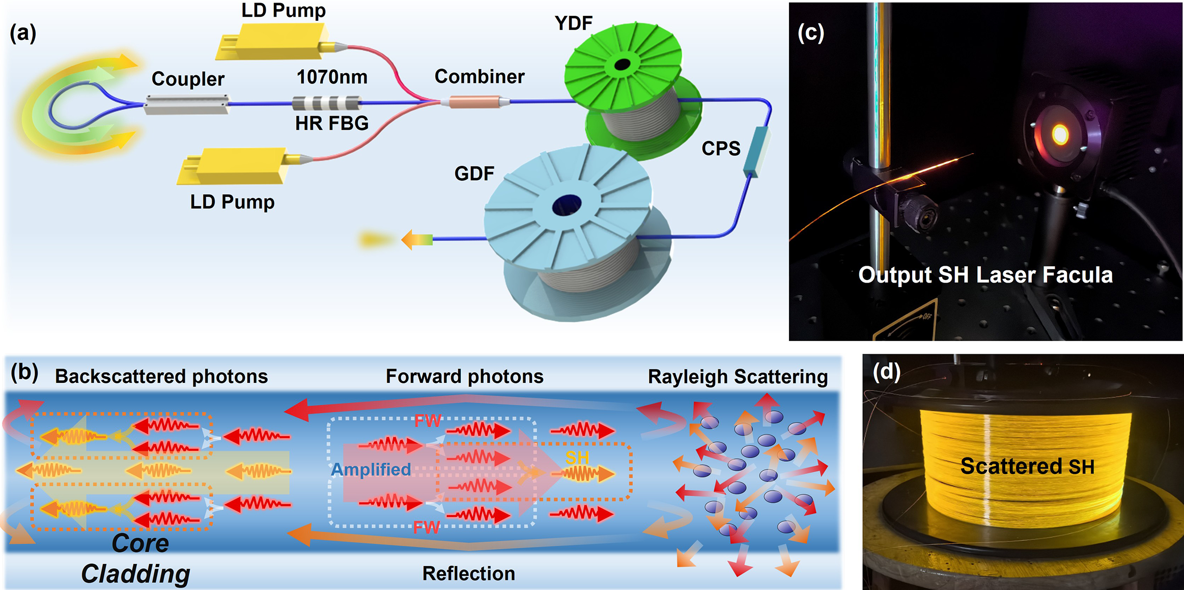
Figure 1 (a) Experimental setup. LD pump, laser diode pump; HR FBG, high-reflectivity fiber Bragg grating; YDF, ytterbium-doped fiber; GDF, germanium-doped fiber; CPS, cladding power stripper. (b) Principle of SH gain and feedback. (c) Output SH laser facula after a cladding light stripper attached to the output. (d) GDF glowing visible light while the pump is injected.
Figure 1(b) illustrates the feedback mechanism in our structure. Rayleigh scattering results in the conversion of a portion of the FW and SH propagating within the fiber into scattered light in multiple directions. A fraction of the scattered light that meets the conditions for total internal reflection is confined within the fiber core. This backscattered light allows the FW to undergo ytterbium ion gain or Raman gain. The backscattered SH can also be amplified. The purpose of employing the FLM is to introduce strong broadband feedback, enabling the reverse propagation of backscattered light for further amplification through both the YDF and germanium-doped fiber (GDF). This setup forms a random cavity via point feedback and distributed feedback, providing feedback for both the FW and SH. Details regarding how the phase-matching conditions are satisfied in the fiber core, as well as other relevant mechanisms, will be given in Section 3. Notably, the FW is generated in the form of pulses. This intentional design stems from the fact that passive spatiotemporal gain modulation within RFLs induces pulsed laser operation[ Reference Xu, Ye, Liu, Wu, Zhang, Leng and Zhou 62 ]. The pulsed FW can significantly augment their peak power and SH conversion efficiency. In addition, the higher power at 1070 nm effectively triggers stronger nonlinear effects, thereby increasing spectral components and facilitating SHG from the FW. Consequently, broadband SHs can be generated without necessitating multiple FW sources. In contrast to injecting the FW laser output into an SH generator, here both the FW and SH are generated within the same scheme, offering superior integration. Also, the continuous operation mode of the LD enhances the pump injection capability, enabling higher average power SHG.
2.2 Evolution of the output spectrum and SH signal power
During the experiment, accompanied by pump injection, a circular visible-light spot can be immediately observed at the output end (Figure 1(c)). This indicates that SHs can be generated, transmitted and output within the fiber core. In addition, scattered visible light from the fiber cladding is also observed (Figure 1(d)). These lights are the SHs in the cladding, for which the phase-matching condition is directly satisfied, that is, the Cherenkov-phase-matched harmonic conversion[ Reference Aparanji, Arun, Balaswamy and Supradeepa 48 ]. Our primary focus is on the SH output directly from the fiber core. To obtain this light spot, a cladding light stripper is connected to the output fiber. The spectrum and power are directly measured at the output end. The measured output spectra at different pump powers are shown in Figure 2. For the structure of the RFL, there exists a sequential relationship. The ytterbium RFL formed by the HR FBG takes precedence, which is in an internal position. Externally, there is the broadband RFL with feedback provided by the FLM. The ytterbium-gain RFL, composed of a 1070 nm HR FBG, ensures the gain priority of 1070 nm light in the YDF, which can enhance the robustness of the system. In addition, the higher optical power at 1070 nm effectively excites nonlinear effects within the GDF, giving rise to increased spectral components and promoting SHG from the FW. Initially, when LD pump power is injected, the ytterbium-gain RFL starts operation, leading to the appearance of a peak at 1070 nm in the output spectrum (Figure 2(a)). At this stage, because the pump power is close to the laser threshold, there are many random noise peaks in the spectrum. They are attributed to the interaction between Rayleigh scattering and stimulated Brillouin scattering effects, which leads to the occurrence of self-Q-switching[ Reference Turitsyn, Babin, El-Taher, Harper, Churkin, Kablukov, Ania-Castañón, Karalekas and Podivilov 63 – Reference Choudhury, Aparanji, Prakash, Balaswamy and Supradeepa 66 ]. The self-Q-switching effect also induces strong pulses in the temporal domain, thereby stimulating the SHG process. The feedback provided by the FLM and Rayleigh scattering forms a random cavity for SHs, hence, besides the noise peaks, there is also a visible peak at 535 nm.
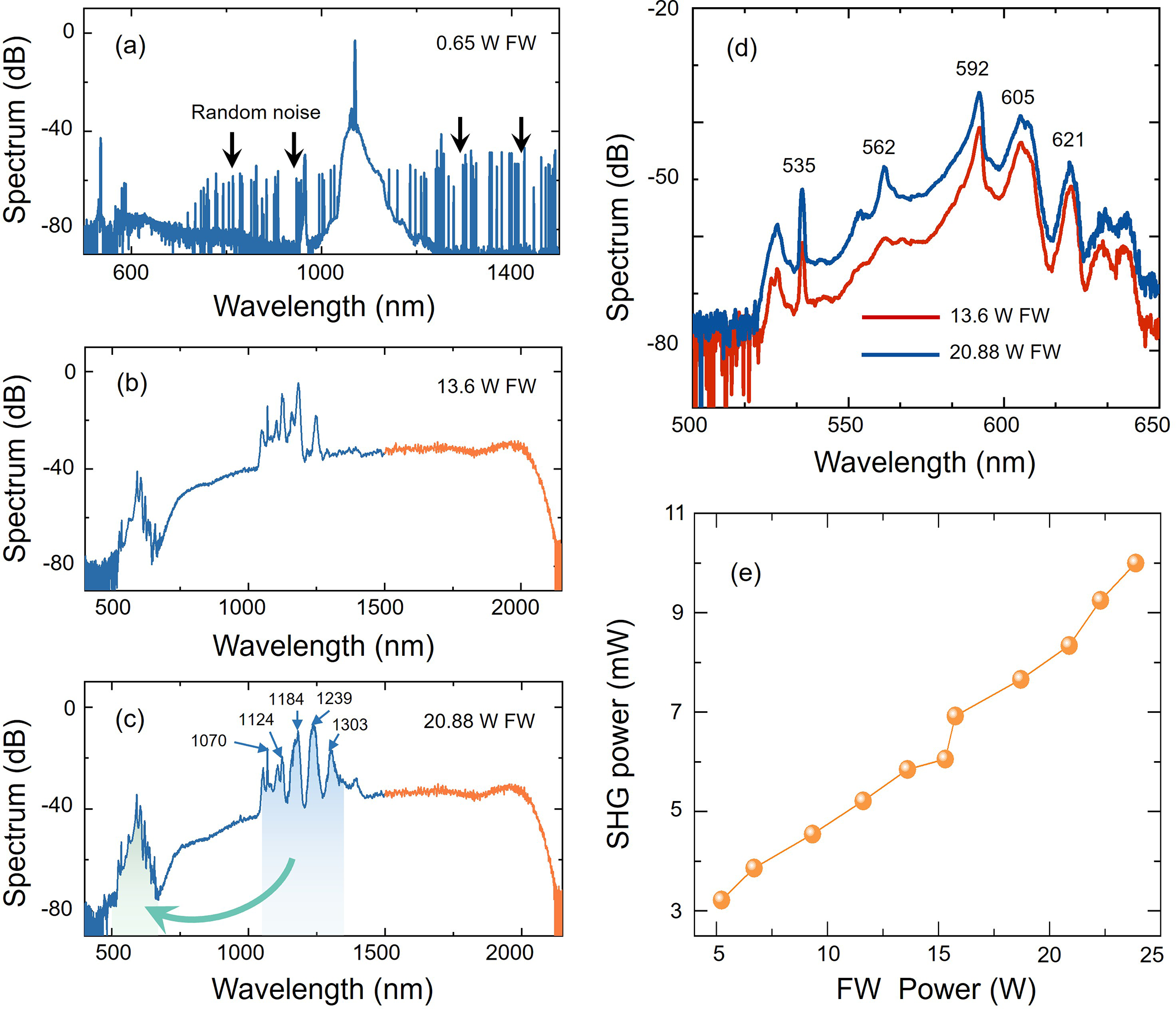
Figure 2 Measured spectra with the FW powers of (a) 0.65 W, (b) 13.6 W and (c) 20.88 W. (d) Comparison of SH band spectra with the FW powers of 13.6 and 20.88 W. (e) The SHG output power with the increase of FW power.
When the LD pump power exceeds the laser threshold and reaches the threshold for cascaded stimulated Raman scattering (SRS) effects (Figure 2(b)), random noise peaks are no longer present. With the pedestal elevating, the spectrum transitions to a supercontinuum. In the near-infrared wavelength range, there are five peaks observed: at 1070 nm and its first-, second- and third-order Stokes lights, as well as a minor peak at 976 nm representing the unabsorbed LD light. The spectrum spans from 680 to 2116 nm. The extension toward shorter wavelengths is attributed to the participation of cascaded SRS Stokes light in cascaded FWM effects[ Reference Lin, Wang, Li, Chen, Rao, Peng and Gomes 49 , Reference Chen, Song, Lei, Yang and Hou 52 ]. Despite the broadening of the spectrum, the intensities of the 1070 nm laser and its cascaded Raman Stokes light exceed the pedestal by tens of dB. These high-intensity lights serve as multi-wavelength FWs for the SHG process and bring about an increase in spectral components in the SH band. The peak at 592 nm becomes predominant rather than that at 535 nm. This phenomenon can be explained as follows: compared to the 535 nm green light, the 592 nm orange light experiences lower losses in the fiber. In addition, a considerable amount of the 1070 nm laser is converted to Raman Stokes light, and the power of the 1184 nm Raman light is sufficient to stimulate SHG. These two conditions lead the 592 nm orange light to dominate the competition.
Figure 2(c) indicates that after the transition to a supercontinuum, further increasing the pump power does not significantly broaden the spectral range. Instead, it promotes energy transfer to higher-order Stokes light and further enhances SHG. In the SH band, the peaks at 535, 561, 592 and 621 nm originate from the 1070 nm light, the first-order SRS Stokes light, the second-order SRS Stokes light and the third-order SRS Stokes light, respectively. The SH band spectrum covers from 520 to 650 nm, spanning 130 nm. Figure 2(d) shows a comparison of SH spectra, showing higher spectrum intensity and more spectral components under 20.88 W FW power. It should be noted that, in our structure, the FW neither undergoes conversion to the third harmonic nor generates other visible-light peaks due to cascaded FWM, phenomena that have been observed in previous studies[ Reference Aparanji, Arun, Balaswamy and Supradeepa 48 , Reference Perret, Fanjoux, Bigot, Fatome, Millot, Dudley and Sylvestre 51 ]. The former is because the fiber used exhibits high loss for the third harmonic corresponding to the FW, placing it at a disadvantage in terms of gain competition. The latter is due to the inability of inter-modal FWM to occur in single-mode fibers. The spectrum of the SH band is not connected to the spectrum of the near-infrared band, which is different from the visible-light spectrum induced by dispersion waves in other studies[ Reference Jiang, Song and Hou 53 ].
By adjusting the power of the pump LD, the evolution of total output power at different pump powers can be measured (see in Note S1 of the Supplementary Material). Furthermore, the SH power at different FW powers is obtained, as depicted in Figure 2(e). The SH power is measured after isolating other optical frequencies using a dichroic mirror and multiple optical filters. The FW powers are determined through spectral integration. The calculation method is shown in Note S2 of the Supplementary Material. At our maximum pump power, the output SH power is 10.06 mW. Further increasing the pump power can generate higher SH power.
2.3 Temporal characteristics of the SH band signal
After separating the light of the SH and FW bands using a dichroic mirror and filters, the waveforms of these two bands are measured separately. The pulse operation characteristic of the FW in this RFL provides the possibility for rapid generation of SHs and causes pulsed behavior of SHs in the temporal domain. The temporal characteristics of the FW are measured, manifesting as pulses with widths of tens of nanoseconds. The pulses arise from passive spatiotemporal gain modulation of the pump light. The pulsed FWs have a repetition rate, although it may fluctuate. As an example at maximum output power, the waveforms of the FW are measured. Due to the wide spectral range, both a Si-based detector (Thorlabs, DET025A) and an InGaAs-based detector (Thorlabs, DET08C) are utilized. According to the measurement results, the waveforms measured by the Si-based detector exhibit a 12 μs pulse repetition period (Figure 3(a)), while those measured by the InGaAs-based detector exhibit a 10 μs period (Figure 3(b)). It should be noted that the waveform period measured with the InGaAs-based detector is unstable with very small fluctuations. The pulses of 1070 nm are rapidly consumed and then generated with a stable period. The energy of the 1070 nm light will be converted to other wavelengths, mainly Raman Stokes light. However, further power consumption involves complex competition among nonlinear effects, which can interfere with the power consumption. More details are shown in Note S3 of the Supplementary Material.
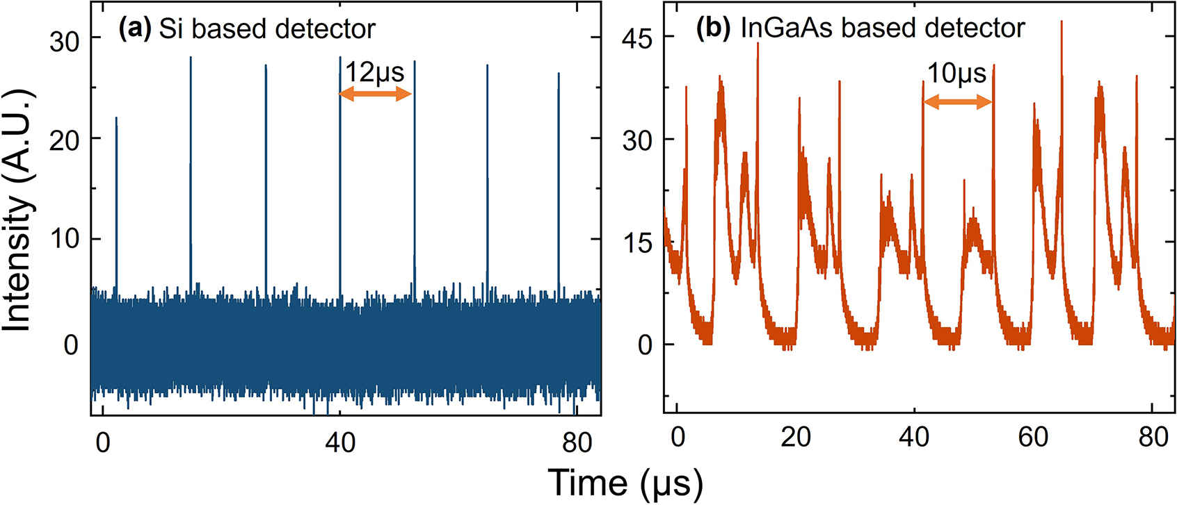
Figure 3 Measured waveforms of the FW by (a) a Si-based detector and (b) an InGaAs-based detector.
Here, we mainly focus on the temporal characteristics of SHs, which cannot be directly measured using Si-based detectors due to the presence of other dispersive waves above 680 nm. Optical filtering devices are used to reduce the stray light spectrum intensity to a negligible level. Figure 4(a) displays the temporal waveforms of SHs under different FW powers, exhibiting significant fluctuations in waveform intensity and the presence of pulses with intensities far exceeding others, suggesting the occurrence of optical rogue waves. The peak voltages of the pulses are extracted as event information and the histograms of the recorded events are plotted to obtain the statistical distribution, as shown in Figure 4(b). The histograms clearly show the L-shaped distribution of optical rogue waves, with the gray area representing noise. The vertical dashed lines indicate the peak amplitude is twice the significant wave height (SWH). The SWH can be defined as the mean height of the highest third of events[ Reference Dudley, Dias, Erkintalo and Genty 67 ]. The appearance of optical rogue waves is unexpected because the intensity fluctuations of the FW are far from being obvious. Moreover, the SH band is also in the normal dispersion region of the fiber, making it difficult for modulation instabilities to appear. We speculate that the possible reason is the dynamic change in the proportion of the FWs participating in the SHG process. The FWs undergo various nonlinear effects, such as SRS, FWM and modulation instabilities simultaneously in the fiber, with dynamic competitive relationships among these effects. Since there is originally a small part of the FW involved in SHG, at certain moments, more FWs participate, and such an increase in proportion is sufficient to significantly enhance the SH waveform intensity. On the other hand, the distribution of signal power itself can also change the distribution of the χ (2), which in turn influences the conversion efficiency, so the perturbation of intensity can be amplified. As the FW power increases, more waveforms with intermediate intensities appear in the histogram, starting to evolve toward a flatter distribution. This implies that further improving the pump power may reduce the probability of rogue wave occurring.
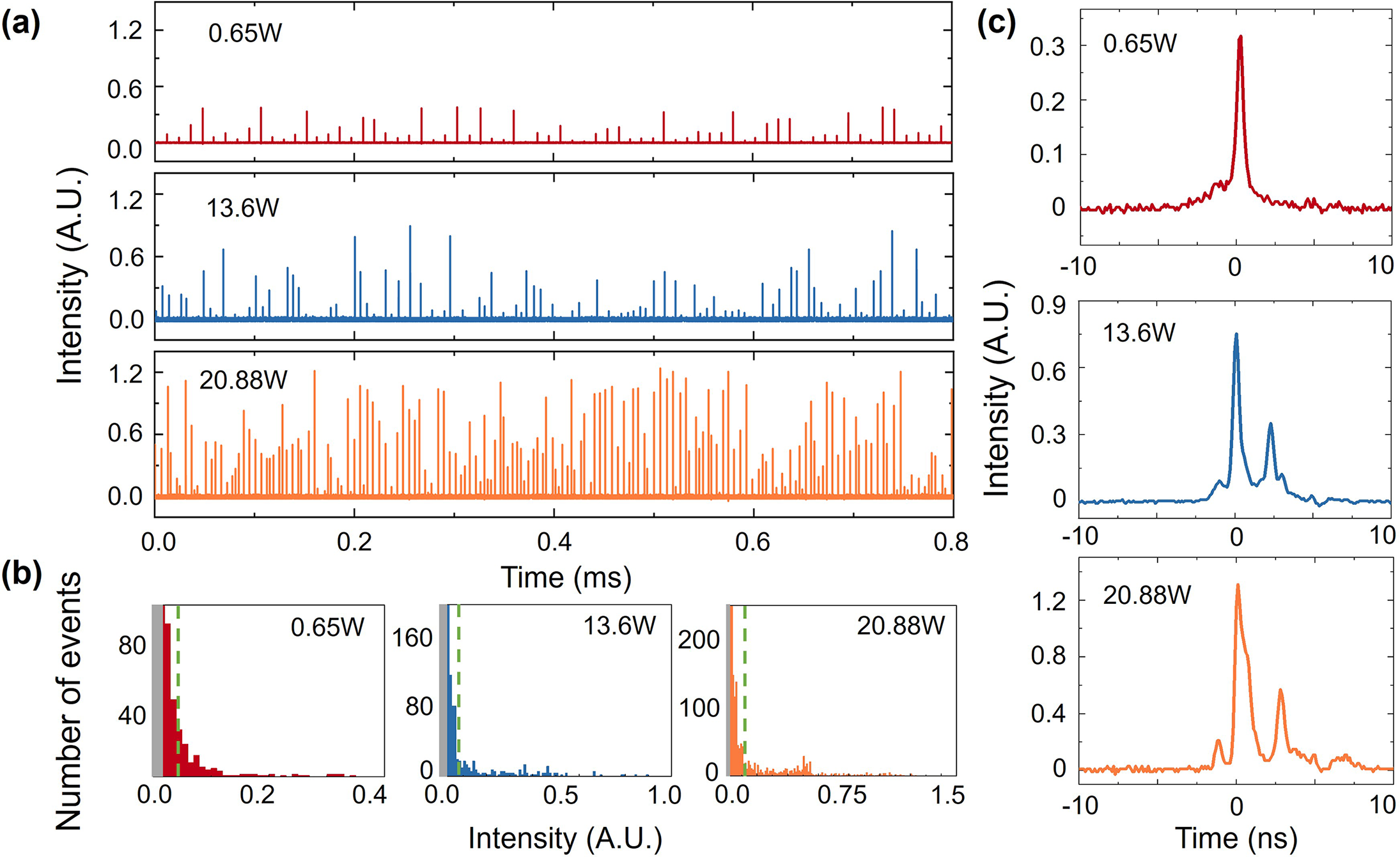
Figure 4 Temporal characteristics of the SH band with different FW powers. (a) Wide time range waveforms. (b) Histogram of the pulse intensity distribution. (c) Single waveform measurement result.
The individual waveform of the rogue waves is depicted in Figure 4(c). It is worth noting that although the pulse widths of the rogue waves are of the order of nanoseconds, the actual widths are likely to be lower and accurate measurement is limited by the bandwidth of the detector. SHG for different FW wavelengths corresponds to χ (2) with different periods. Therefore, SHs of different wavelengths are generated at different positions within the fiber, resulting in slight differences in the output timing. As can also be observed in Figure 4(c), when the FW power increases, additional pulse peaks appear beside the main peak, which can be treated as the SH from other FWs with lower intensity.
3 Discussion
Next, we perform a simulation analysis of our experimental results. In terms of the cladding SH, it is already the subject of in-depth studies[
Reference Aparanji, Arun, Balaswamy and Supradeepa
48
]. Our focus is primarily on the in-core SH, as it exhibits better beam quality. There are two key reasons that this RFL can generate the in-core SH efficiently rather than completely depleting it. Firstly, the SH has received sufficient feedback. The point feedback and distributed feedback form a random cavity. The feedback band covers the SH band, allowing a portion of the scattered SH to return to the passive fiber for amplification. Secondly, due to the passive spatiotemporal modulation of the pump light in the half-open cavity structure, the FW propagates in the form of pulsed light, with high peak power enhancing the SH gain. To verify the influence of these two factors, a theoretical model is established based on the self-organized SHG theory[
Reference Antonyuk
68
]. This theory links induced χ
(2) with the presence of germanium dopants, which lead to the appearance of defects that trap electrons. The electrons are transferred from Ge-centers to a silica matrix or to a different Ge-center under pumping[
Reference Majchrowska, Pabisiak, Martynkien, Mergo and Tarnowski
33
]. These electrons are referred to as charge transfer excitons (CTEs)[
Reference Antonyuk and Antonyuk
31
]. The delocalization of charges enhances χ
(2), and amplifies the polarization ${P}_\mathrm{dc}^0$
and the corresponding field
${P}_\mathrm{dc}^0$
and the corresponding field ${E}_\mathrm{dc}^0$
. The periodic electric field participates in and drives the SHG process. The excitation of the electric field is associated with FW injection and one photon absorption of the SH[
Reference Antonyuk and Antonyuk
31
]. In our structure, the initial SHG can arise from various mechanisms, including the surface nonlinearity of the fiber core cladding interface, the nonlinearity derived from the electric quadrupole moment or the magnetic dipole moment and the SH in the cladding, which is generated based on Cherenkov-type radiation phase-matching.
${E}_\mathrm{dc}^0$
. The periodic electric field participates in and drives the SHG process. The excitation of the electric field is associated with FW injection and one photon absorption of the SH[
Reference Antonyuk and Antonyuk
31
]. In our structure, the initial SHG can arise from various mechanisms, including the surface nonlinearity of the fiber core cladding interface, the nonlinearity derived from the electric quadrupole moment or the magnetic dipole moment and the SH in the cladding, which is generated based on Cherenkov-type radiation phase-matching.
The amplitudes ${A}_0$
,
${A}_0$
, ${A}_1$
,
${A}_1$
, ${A}_2$
and phases
${A}_2$
and phases ${\psi}_0$
,
${\psi}_0$
, ${\psi}_1$
,
${\psi}_1$
, ${\psi}_2$
of static, fundamental and SH fields are introduced, respectively, as variables. The corresponding physical fields are as follows[
Reference Antonyuk
68
]:
${\psi}_2$
of static, fundamental and SH fields are introduced, respectively, as variables. The corresponding physical fields are as follows[
Reference Antonyuk
68
]:
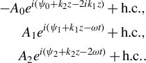 $$\begin{align}-{A}_0{e}^{i\left({\psi}_0+{k}_2z-2{ik}_1z\right)}+\mathrm{h.c.},\nonumber\\ {}{A}_1{e}^{i\left({\psi}_1+{k}_1z-\omega t\right)}+\mathrm{h.c.},\nonumber\\ {}{A}_2{e}^{i\left({\psi}_2+{k}_2z-2\omega t\right)}+\mathrm{h.c.}.\\[-18pt]\nonumber\end{align}$$
It can be seen that the phase-matching condition is automatically satisfied through this electric field. For the electric field, its saturated form should be a solution of the following equation:
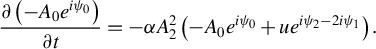 $$\begin{align}\frac{\partial \left(-{A}_0{e}^{i{\psi}_0}\right)}{\partial t}=-\alpha {A}_2^2\left(-{A}_0{e}^{i{\psi}_0}+{ue}^{i{\psi}_2-2i{\psi}_1}\right).\\[-18pt]\nonumber \end{align}$$
For the fundamental and SH fields, the wave equations for slow variables are as follows:
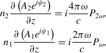 $$\begin{align}{n}_2\frac{\partial \left({A}_2{e}^{i{\psi}_2}\right)}{\partial z}=i\frac{4\pi \omega}{c}{P}_{2\omega },\nonumber\\ {}{n}_1\frac{\partial \left({A}_1{e}^{i{\psi}_1}\right)}{\partial z}=i\frac{2\pi \omega}{c}{P}_{\omega },\end{align}$$
where ${P}_{2\omega }$
and
${P}_{2\omega }$
and ${P}_{\omega }$
are ordinary
${P}_{\omega }$
are ordinary ${\chi}^{(3)}$
nonlinear terms:
${\chi}^{(3)}$
nonlinear terms:
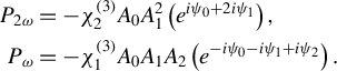 $$\begin{align}{P}_{2\omega}&=-{\chi}_2^{(3)}{A}_0{A}_1^2\left({e}^{i{\psi}_0+2i{\psi}_1}\right),\nonumber\\ {}{P}_{\omega}&=-{\chi}_1^{(3)}{A}_0{A}_1{A}_2\left({e}^{-i{\psi}_0-i{\psi}_1+i{\psi}_2}\right).\end{align}$$
Thus,
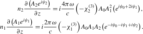 $$\begin{align}{n}_2\frac{\partial \left({A}_2{e}^{i{\psi}_2}\right)}{\partial z}=i\frac{4\pi \omega}{c}\left(-{\chi}_2^{(3)}\right){A}_0{A}_1^2\left({e}^{i{\psi}_0+2i{\psi}_1}\right),\nonumber\\ {}{n}_1\frac{\partial \left({A}_1{e}^{i{\psi}_1}\right)}{\partial z}=i\frac{2\pi \omega}{c}\left(-{\chi}_1^{(3)}\right){A}_0{A}_1{A}_2\left({e}^{-i{\psi}_0-i{\psi}_1+i{\psi}_2}\right).\end{align}$$
The final equations for normalized variables are as follows:
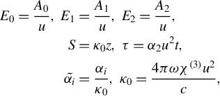 $$\begin{align}{E}_0=\frac{A_0}{u},\kern0.36em {E}_1&=\frac{A_1}{u},\kern0.36em {E}_2=\frac{A_2}{u},\nonumber\\ {}S&={\kappa}_0z,\kern0.36em \tau ={\alpha}_2{u}^2t,\nonumber\\ {}\tilde{\alpha_i}&=\frac{\alpha_i}{\kappa_0},\kern0.36em {\kappa}_0=\frac{4{\pi \omega \chi}^{(3)}{u}^2}{c},\end{align}$$
following from Equations (S2) and (S4) in the Supplementary Material. There are the following[ Reference Antonyuk 68 ]:
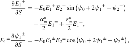
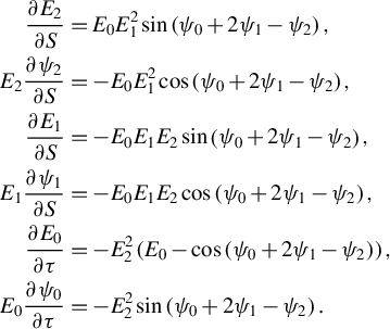 $$\begin{align}\frac{\partial {E}_2}{\partial S}&={E}_0{E}_1^2\sin \left({\psi}_0+2{\psi}_1-{\psi}_2\right),\nonumber\\ {}{E}_2\frac{\partial {\psi}_2}{\partial S}&=-{E}_0{E}_1^2\cos \left({\psi}_0+2{\psi}_1-{\psi}_2\right),\nonumber\\ {}\frac{\partial {E}_1}{\partial S}&=-{E}_0{E}_1{E}_2\sin \left({\psi}_0+2{\psi}_1-{\psi}_2\right),\nonumber\\ {}{E}_1\frac{\partial {\psi}_1}{\partial S}&=-{E}_0{E}_1{E}_2\cos \left({\psi}_0+2{\psi}_1-{\psi}_2\right),\nonumber\\ {}\frac{\partial {E}_0}{\partial \tau}&=-{E}_2^2\left({E}_0-\cos \left({\psi}_0+2{\psi}_1-{\psi}_2\right)\right),\nonumber\\ {}{E}_0\frac{\partial {\psi}_0}{\partial \tau}&=-{E}_2^2\sin \left({\psi}_0+2{\psi}_1-{\psi}_2\right).\end{align}$$
In our modified model, the distributed feedback provided by Rayleigh scattering is introduced. Naturally, it is necessary to distinguish between forward and backward light in the fiber, both for the SH and the FW. To simplify the model, forward and backward SHs are assumed to originate solely from forward and backward FWs, respectively. In addition, fiber losses for both the SH and the FW are taken into account, as this involves losses within the cavity. The equations are as follows:
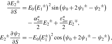 $$\begin{align}\frac{\partial {E_2}^{\pm }}{\partial S}&={E}_0{\left({E_1}^{\pm}\right)}^2\sin \left({\psi}_0+2{\psi_1}^{\pm }-{\psi_2}^{\pm}\right)\nonumber\\ &\quad-\frac{\alpha_{2\omega}^n}{2}{E_2}^{\pm }+\frac{\varepsilon_{2\omega}^n}{2}{E_2}^{\mp },\nonumber\\ {}{E_2}^{\pm}\frac{\partial {\psi}_2}{\partial S}&=-{E}_0{\left({E}_1^{\pm}\right)}^2\cos \left({\psi}_0+2{\psi_1}^{\pm }-{\psi_2}^{\pm}\right),\end{align}$$
 $$\begin{align}\frac{\partial {E_1}^{\pm }}{\partial S}&=-{E}_0{E_1}^{\pm }{E_2}^{\pm}\sin \left({\psi}_0+2{\psi_1}^{\pm }-{\psi_2}^{\pm}\right)\nonumber\\&\quad -\frac{\alpha_{\omega}^n}{2}{E_1}^{\pm }+\frac{\varepsilon_{\omega}^n}{2}{E_1}^{\mp },\nonumber\\ {}{E_1}^{\pm}\frac{\partial {\psi_1}^{\pm }}{\partial S}&=-{E}_0{E_1}^{\pm }{E_2}^{\pm}\cos \left({\psi}_0+2{\psi_1}^{\pm }-{\psi_2}^{\pm}\right),\\[-50pt]\nonumber\end{align}$$
 $$\begin{align}\frac{\partial {E}_0}{\partial \tau}&=-{\left({E_2}^{\pm}\right)}^2\left({E}_0-\cos \left({\psi}_0+2{\psi_1}^{\pm }-{\psi_2}^{\pm}\right)\right),\nonumber\\ {}{E}_0\frac{\partial {\psi}_0}{\partial \tau}&=-{\left({E_2}^{\pm}\right)}^2\sin \left({\psi}_0+2{\psi_1}^{\pm }-{\psi_2}^{\pm}\right),\end{align}$$
where ${\alpha}_{2\omega}^n$
and
${\alpha}_{2\omega}^n$
and ${\alpha}_{\omega}^n$
represent the normalized loss terms for the SH and FW, respectively, and
${\alpha}_{\omega}^n$
represent the normalized loss terms for the SH and FW, respectively, and ${\varepsilon}_{2\omega}^n$
and
${\varepsilon}_{2\omega}^n$
and ${\varepsilon}_{\omega}^n$
denote the coefficients of Rayleigh scattering light of the SH and FW being total-reflected. The cavity is formed through distributed feedback and point feedback. Distributed feedback is manifested through the Rayleigh scattering term, while point feedback is reflected at the boundaries. More detailed explanations about this model can be found in Note S4 of the Supplementary Material. Utilizing the modified self-organized SHG model, under the same pumping and initial conditions, the evolution of the SH in both the fiber without FLM feedback and the half-open cavity RFL is analyzed. This part of the simulation is also shown in Note S4 of the Supplementary Material.
${\varepsilon}_{\omega}^n$
denote the coefficients of Rayleigh scattering light of the SH and FW being total-reflected. The cavity is formed through distributed feedback and point feedback. Distributed feedback is manifested through the Rayleigh scattering term, while point feedback is reflected at the boundaries. More detailed explanations about this model can be found in Note S4 of the Supplementary Material. Utilizing the modified self-organized SHG model, under the same pumping and initial conditions, the evolution of the SH in both the fiber without FLM feedback and the half-open cavity RFL is analyzed. This part of the simulation is also shown in Note S4 of the Supplementary Material.
However, for the FW, it is inaccurate to consider only its loss and assume that the FW is just directly injected into the fiber. This is because the FW is generated from the same RFL, and its energy will spread to a wider frequency range. By incorporating FW gain and conversion to other wavelengths, a more precise evolution of the SH field within this RFL can be provided. A detailed theoretical model is based on the GNLSEs, taking the dispersion effect, self-phase modulation, cross-phase modulation, cascaded Raman scattering, average Rayleigh scattering and SHG into account:
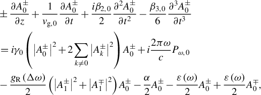 $$\begin{align}&\pm \frac{\partial {A}_0^{\pm }}{\partial z}+\frac{1}{v_{\mathrm{g},0}}\frac{\partial {A}_0^{\pm }}{\partial t}+\frac{i{\beta}_{2,0}}{2}\frac{\partial^2{A}_0^{\pm }}{\partial {t}^2}-\frac{\beta_{3,0}}{6}\frac{\partial^3{A}_0^{\pm }}{\partial {t}^3}\nonumber\\ &=i{\gamma}_0\left({\left|{A}_0^{\pm}\right|}^2+2\sum\limits_{k\ne 0}{\left|{A}_k^{\pm}\right|}^2\right){A}_0^{\pm }+i\frac{2\pi \omega}{c}{P}_{\omega, 0}\nonumber\\ &{}-\frac{g_\mathrm{R}\left(\varDelta \omega \right)}{2}\left({\left|{A}_1^{\pm}\right|}^2+{\left|{A}_1^{\mp}\right|}^2\right){A}_0^{\pm }-\frac{\alpha }{2}{A}_0^{\pm }-\frac{\varepsilon \left(\omega \right)}{2}{A}_0^{\pm }+\frac{\varepsilon \left(\omega \right)}{2}{A}_0^{\mp },\\[-52pt]\nonumber\end{align}$$
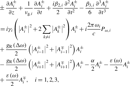 $$\begin{align}&\pm \frac{\partial {A}_i^{\pm }}{\partial z}+\frac{1}{v_{\mathrm{g},i}}\frac{\partial {A}_i^{\pm }}{\partial t}+\frac{i{\beta}_{2,i}}{2}\frac{\partial^2{A}_i^{\pm }}{\partial {t}^2}-\frac{\beta_{3,i}}{6}\frac{\partial^3{A}_i^{\pm }}{\partial {t}^3}\nonumber\\ &=i{\gamma}_i\left({\left|{A}_i^{\pm}\right|}^2+2\sum\limits_{k\ne i}{\left|{A}_k^{\pm}\right|}^2\right){A}_i^{\pm }+i\frac{2{\pi \omega}_i}{c}{P}_{\omega, i}\nonumber\\ &{}+\frac{g_\mathrm{R}\left(\varDelta \omega \right)}{2}\left({\left|{A}_{i-1}^{\pm}\right|}^2+{\left|{A}_{i-1}^{\mp}\right|}^2\right){A}_i^{\pm }\nonumber\\ &-\frac{g_\mathrm{R}\left(\varDelta \omega \right)}{2}\left({\left|{A}_{i+1}^{\pm}\right|}^2+{\left|{A}_{i+1}^{\mp}\right|}^2\right){A}_i^{\pm }-\frac{\alpha }{2}{A}_i^{\pm }-\frac{\varepsilon \left(\omega \right)}{2}{A}_i^{\pm}\nonumber\\ &{}+\frac{\varepsilon \left(\omega \right)}{2}{A}_i^{\mp },\quad i=1,2,3,\end{align}$$
 $$\begin{align}&\pm \frac{\partial {A}_4^{\pm }}{\partial z}+\frac{1}{v_{\mathrm{g},4}}\frac{\partial {A}_4^{\pm }}{\partial t}+\frac{i{\beta}_{2,4}}{2}\frac{\partial^2{A}_4^{\pm }}{\partial {t}^2}-\frac{\beta_{3,4}}{6}\frac{\partial^3{A}_4^{\pm }}{\partial {t}^3}\nonumber\\ &=i{\gamma}_4\left({\left|{A}_4^{\pm}\right|}^2+2\sum\limits_{k\ne 4}{\left|{A}_k^{\pm}\right|}^2\right){A}_4^{\pm }+i\frac{2{\pi \omega}_4}{c}{P}_{\omega, 4}\nonumber\\ &{}+\frac{g_\mathrm{R}\left(\varDelta \omega \right)}{2}\left({\left|{A}_3^{\pm}\right|}^2+{\left|{A}_3^{\mp}\right|}^2\right){A}_4^{\pm }-\frac{\alpha }{2}{A}_4^{\pm }\nonumber\\ &-\frac{\varepsilon \left(\omega \right)}{2}{A}_4^{\pm }+\frac{\varepsilon \left(\omega \right)}{2}{A}_4^{\mp }, \end{align}$$
where $A$
is the complex amplitude of the optical field and superscripts + and − represent the forward and backward propagating lights. The subscripts 0–4 denote the 1070 nm light, the 1120 nm first-order Stokes wave, the 1178 nm second-order Stokes wave, the 1243 nm third-order Stokes wave and the 1310 nm fourth-order Stokes wave, respectively, while
$A$
is the complex amplitude of the optical field and superscripts + and − represent the forward and backward propagating lights. The subscripts 0–4 denote the 1070 nm light, the 1120 nm first-order Stokes wave, the 1178 nm second-order Stokes wave, the 1243 nm third-order Stokes wave and the 1310 nm fourth-order Stokes wave, respectively, while ${v}_\mathrm{g}$
is the group velocity,
${v}_\mathrm{g}$
is the group velocity, ${\beta}_2$
and
${\beta}_2$
and ${\beta}_3$
are the second- and third-order dispersion coefficients, respectively,
${\beta}_3$
are the second- and third-order dispersion coefficients, respectively, $\gamma$
is the nonlinear parameter,
$\gamma$
is the nonlinear parameter, ${g}_\mathrm{R}\left(\varDelta \omega \right)$
is the Raman gain of different frequency shifts,
${g}_\mathrm{R}\left(\varDelta \omega \right)$
is the Raman gain of different frequency shifts, $\alpha$
is the loss coefficient and
$\alpha$
is the loss coefficient and $\varepsilon (\omega)$
is the Rayleigh scattering coefficient of different wavelengths. It should be noted that the second term on the right-hand side of Equations (4)–(6) represents the conversion of the FW to the SH, and this term is equivalent to Equation (2). Therefore, together with Equations (1) and (3), we can simulate the simultaneous evolution of the FW and SH in our structure.
$\varepsilon (\omega)$
is the Rayleigh scattering coefficient of different wavelengths. It should be noted that the second term on the right-hand side of Equations (4)–(6) represents the conversion of the FW to the SH, and this term is equivalent to Equation (2). Therefore, together with Equations (1) and (3), we can simulate the simultaneous evolution of the FW and SH in our structure.
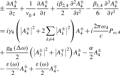
The simulated output spectrum of the FW is shown in Figure 5(a). Several main spectral peaks align with the experimental results. The evolution of the spectrum along the fiber is shown in Figure 5(b). The energy of the 1070 nm light quickly converts to Raman light.
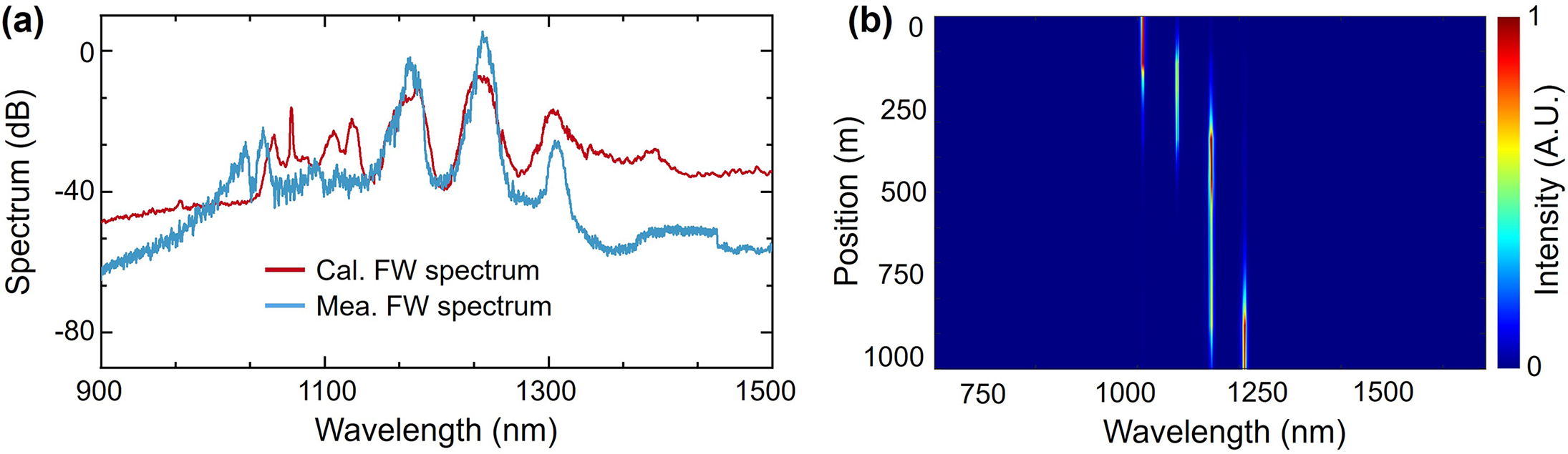
Figure 5 Simulated (a) output spectrum and (b) spectral evolution along the passive fiber of the FW.
The evolutions of the SH spectrum and the final output spectrum are shown in Figures 6(a) and 6(b). The intensity of the FW is a determining factor for SH gain. FWs that do not rapidly convert to other wavelengths correspond to stronger SH gain. According to the simulation results, the frequency-doubled light of the first-, second- and third-order Stokes waves dominates. However, the simulated pedestal is lower, which is because the pedestal is primarily generated by nonlinear interactions between different wavelengths. In our model, the nonlinear effects within the SH band itself were not considered. Figure 6(c) shows the SH conversion efficiency for different lengths of GDF, with the highest conversion efficiency occurring around 1000 m, which is why experiments are conducted at this length.
Figure 6 Simulated (a) output spectrum and (b) spectral evolution along the passive fiber of the SH. (c) The SH conversion efficiency with different GDF lengths.
To verify whether the FLM provides feedback to the SH, its internal spectrum is also measured. Employing a 99/1 coupler, a portion of the internal light is extracted and measured. The visible-light spectrum indicates that point feedback plays a role, as detailed in Note S5 of the Supplementary Material. Furthermore, simulation analysis shows that the feedback intensity of point feedback can influence the SH power; however, SHG can still occur even when the feedback intensity is weakened. Using a long fiber, we explore another possibility for providing backward light feedback. This is also distributed feedback, where the feedback for visible light is stronger than that for near-infrared light. The laser structure and output spectra are presented in Note S6 of the Supplementary Material. The SH components demonstrate that effective SHG occurs even under weak feedback conditions. Thus, the structure for achieving in-core SHG using an all-fiber RFL can be diverse.
4 Conclusion
In summary, we introduce a broadband-distributed feedback RFL capable of realizing an in-core second-order nonlinear process, specifically SHG. The passive spatiotemporal gain modulation of the RFL and the extended fiber enhances the SH gain. The random cavity for the SH is formed by distributed feedback and point feedback. A maximum output power of 10.06 mW for the SH band is realized. Temporal analyses reveal the occurrence of optical rogue waves, with statistical analysis indicating that higher pump power may be able to mitigate the probability of their appearance. A theoretical model for SHG in the RFL is shown, and further coupled with the GNLSEs to solve the broad-spectrum evolution more accurately. Our research introduces an all-fiber in-core SHG approach that requires no special treatment and exhibits strong pumping injection capability. Moreover, this structure can simultaneously generate FWs and SHs, offering a highly integrated design. Further studies might include the design of feedback response for SH wavelength tuning, increasing pump power for higher-power applications and in-depth investigation of rogue waves. We believe the simple method we demonstrate for generating in-core SHs may be able to support further research on in-core second-order nonlinear effects and RFLs.
Supplementary material
The supplementary material for this article can be found at http://doi.org/10.1017/hpl.2025.25.
Acknowledgement
This work is supported by the Beijing Natural Science Foundation (Grant No. L241021), the National Key Research and Development Program of China (Grant No. 2023YFB4604501) and the National Natural Science Foundation of China (Grant Nos. 62475132 and 62122040).


 Open access