


1 Introduction
With the development of chirped pulse amplification (CPA)[ Reference Strickland and Mourou1] and optical parametric CPA (OPCPA)[ Reference Dubietis, Jonusauskas and Piskarskas2], ultrahigh-power lasers have been generated worldwide, which can be widely used in high-order harmonic generation[ Reference Ghimire and Reis3], particle acceleration[ Reference Hooker4], vacuum birefringence[ Reference Heinzl, Liesfeld, Amthor, Schwoerer, Sauerbrey and Wipf5], strong-field quantum electrodynamics and even the generation of positron–electron pairs from vacuum[ Reference Cartlidge6, Reference Cartlidge7]. Nowadays, laser facilities of tens of PW level have been built in China[ Reference Gan, Yu, Wang, Liu, Xu, Li, Li, Yu, Wang, Liu, Chen, Peng, Xu, Yao, Zhang, Chen, Tang, Wang, Yin, Liang, Leng, Li, Xu, Yamanouchi, Midorikawa and Roso8] and Romania[ Reference Lureau, Matras, Chalus, Derycke, Morbieu, Radier, Casagrande, Laux, Ricaud, Rey, Pellegrina, Richard, Boudjemaa, Simon-Boisson, Baleanu, Banici, Gradinariu, Caldararu, De Boisdeffre, Ghenuche, Naziru, Kolliopoulos, Neagu, Dabu, Dancus and Ursescu9], and laser facilities of even hundreds of PW level are under construction in China[ Reference Wu, Hu, Liu, Zhang, Bai, Wang, Zhao, Yang, Xu, Wang, Leng and Li10], Russia[ Reference Khazanov, Shaykin, Kostyukov, Ginzburg, Mukhin, Yakovlev, Soloviev, Kuznetsov, Mironov, Korzhimanov, Bulanov, Shaikin, Kochetkov, Kuzmin, Martyanov, Lozhkarev, Starodubtsev, Litvak and Sergeev11] and the United States[ Reference Zuegel, Di Piazza, Dollar, Aprahamian, Zurek and Hill12].
The stretcher, amplifier and compressor are three key components in PW laser systems, of which the compressor is the main limitation of the output peak power currently, as the comprised gratings in the compressor are limited in both damage threshold and size. Generally, spatial intensity modulation exists in amplified laser beams, and for the operational safety of the compressor, its output peak power should be kept lower than almost half of the damage threshold of the last grating in it.
Tiled gratings[ Reference Liang, Du, Chen, Wu, Shen, Wang, Liu and Li13] and the multi-beam tiled-aperture combing method[ Reference Blanchot, Marre, Néauport, Sibé, Rouyer, Montant, Cotel, Le Blanc and Sauteret14] were proposed to increase output peak power for PW laser facilities[ Reference Khazanov, Shaykin, Kostyukov, Ginzburg, Mukhin, Yakovlev, Soloviev, Kuznetsov, Mironov, Korzhimanov, Bulanov, Shaikin, Kochetkov, Kuzmin, Martyanov, Lozhkarev, Starodubtsev, Litvak and Sergeev11]. However, the difficulty lies in the adjustment of the adjacent sub-gratings for tiled gratings, and temporal delay, wavefront, dispersion and pointing stability control of the beams for multi-beam tiled-aperture combining[ Reference Leshchenko15, Reference Zhu, van Howe, Durst, Zipfel and Xu16].
Another method to improve the output peak power is introducing spatial dispersion by simply tuning the distance of grating pairs. Different from the traditional Treacy compressor (TC)[ Reference Treacy17] or symmetric four-grating compressor (FGC), a certain amount of spatial dispersion is introduced in the asymmetric four-grating compressor (AFGC) to smooth the output pulse spatial intensity modulation in the X direction (perpendicular to the grating groove). The AFGC was proposed in 2007[ Reference Huang and Kessler18] but was not urgent at that time. Nowadays, the AFGC is actively studied[ Reference Shen, Du, Liang, Wang, Liu and Li19– Reference Liang, Du, Chen, Wang, Liu, Chen, Shen, Liu and Li21]. However, the smoothing in the X direction has little effect on modulation of the Y direction (parallel to the grating groove).
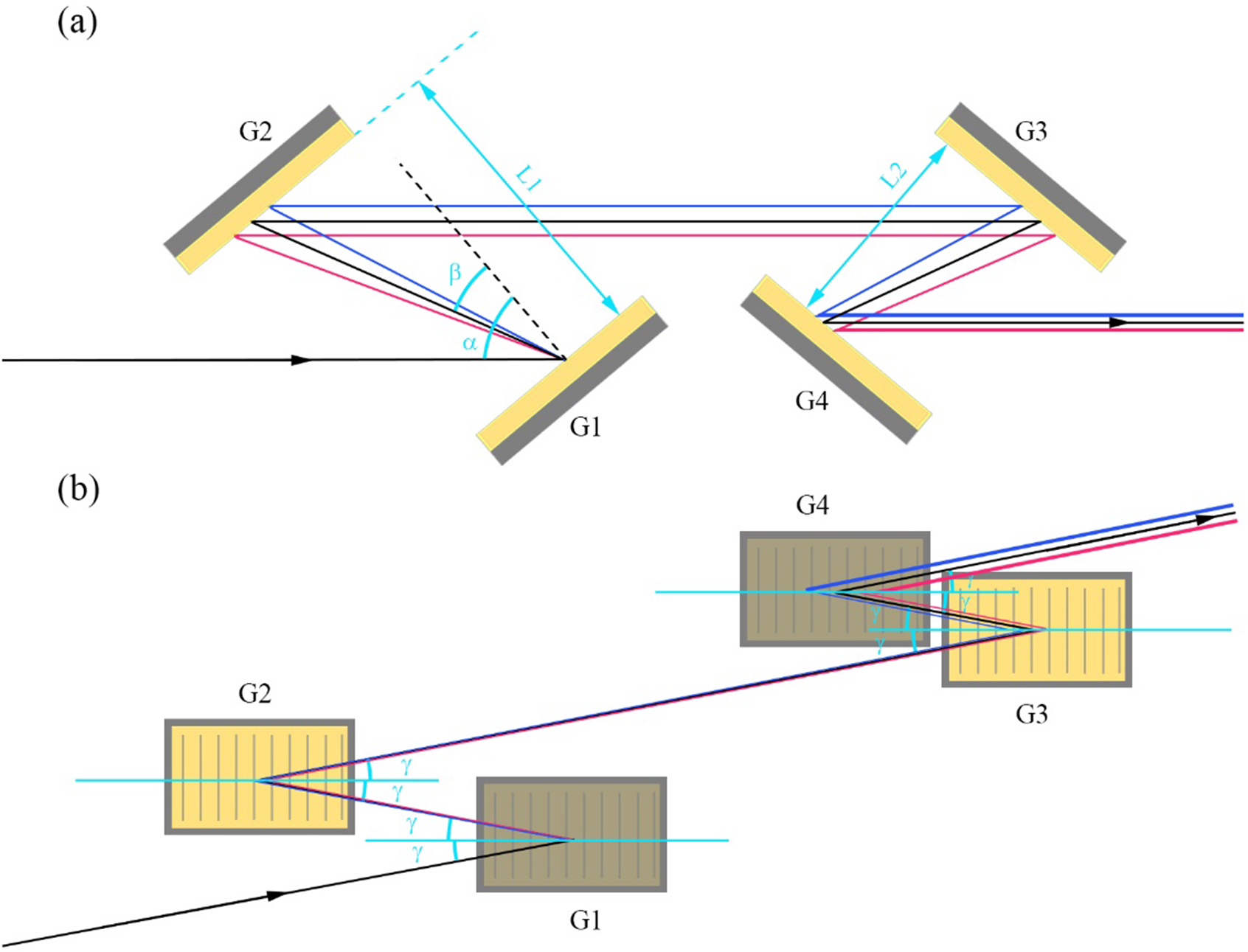
Figure 1 Setup of the DSGC. (a) Top view of the setup. G1–G4 are 1480 lines/mm, 800 nm central wavelength golden gratings; $\alpha$
and
$\alpha$
and $\beta$
are the incident angle and diffraction angle, respectively. (b) Side view of the setup;
$\beta$
are the incident angle and diffraction angle, respectively. (b) Side view of the setup; $\gamma$
is the out-of-plane angle.
$\gamma$
is the out-of-plane angle.
By introducing out-of-plane design between the incident light and the plane perpendicular to the grating line, the out-of-plane compressor (OC)[ Reference Osvay and Ross22] has the ability to smooth the spatial modulation in the Y direction[ Reference Khazanov23]. Along with the developed grating making technology, even with an out-of-plane angle of 15°, the diffraction efficiency can almost remain undiminished, with unaffected pulse temporal and spatial characteristics.
The dispersion of the OC has been analyzed in detail previously[ Reference Li, Rao, Leng, Chen and Dai24]. Further applications of the OC such as an OC with Littrow incident angle[ Reference Kalinchenko, Vyhlidka, Kramer, Lerer and Rus25, Reference Khazanov26] and ultra-broadband grating compressor[ Reference Han, Li, Zhang, Kong, Cao, Jin, Leng, Li and Shao27], have been proposed. Diffraction mechanisms of grating introducing different kinds of out-of-plane angles have also been studied recently[ Reference Smith, Erdogan and Erdogan28]. Several experiments of the OC have been done[ Reference Vyhlídka, Trojek, Kramer, Peceli, Batysta, Bartonícek, Hubácek, Borger, Antipenkov, Gaul, Ditmire and Rus29, Reference Werle, Braun, Eichner, Hülsenbusch, Palmer and Maier30]. Using the OC for beam smoothing in the Y direction was proposed in Ref. [Reference Khazanov23], where theoretical formulas were derived systematically. The Y-smoothing grating compressor (YSGC)[ Reference Khazanov23] (one sort of OC) with longitudinal smoothing ability is achieved by introducing out-of-plane angles in the compressor, as shown in Figure 1(b). Also in Ref. [Reference Khazanov23] the double-smoothing grating compressor (DSGC) was proposed for beam smoothing in the X and Y directions. Experimental research of the DSGC is limited by the proof-of-principle experiment[ Reference Kiselev, Kochetkov, Yakovlev and Khazanov31], where the two-dimensional spectra of the fluence fluctuation were measured and its comparison with the theoretical one gave good quantitative agreement.
In this study, with a home-made FGC, simulation and experiment of the DSGC, which combines the AFGC and the YSGC, were conducted. The results demonstrate that the spatial intensity modulation is greatly weakened without deteriorating the temporal and spatial characteristics.
2 Principles of the double-smoothing grating compressor
2.1 Temporal compression
Figure 1 schematically depicts the top and side views of the DSGC configuration. The input beam is an amplified uncompressed 10th-order super-Gaussian pulse with positive chirp, as Equation (1) shows:
 $$\begin{align}E=\sqrt{I_0}\ \mathit{\exp}\left(-{r}^{10}/{r}_0^{10}\right)\times \mathit{\exp}\left(-1- iC/2\right){\left(t/{T}_0\right)}^2.\end{align}$$
The chirp parameter $C>0$
corresponds to a pulse exhibiting a positive frequency chirp. If we neglect diffraction effects, the temporal and spatial dispersion introduced by the DSGC can be expressed as follows:
$C>0$
corresponds to a pulse exhibiting a positive frequency chirp. If we neglect diffraction effects, the temporal and spatial dispersion introduced by the DSGC can be expressed as follows:
 $$\begin{align}\phi \left(\omega,\, {k}_x,\,{k}_y\right)={\phi}_0+{\phi}^{\prime}\Omega +\frac{\phi^{\prime \prime }}{2}{\Omega}^2+\frac{\phi^{\prime \prime \prime }}{6}{\Omega}^3+{\tau}_x\frac{k_x}{k_0}\Omega +{\tau}_y\frac{k_y}{k_0}\Omega. \end{align}$$
In Equation (2), $\phi \left(\omega \right)$
represents the phase delay of different frequencies, where
$\phi \left(\omega \right)$
represents the phase delay of different frequencies, where $\Omega =\omega -{\omega}_0$
is the frequency difference from the central frequency
$\Omega =\omega -{\omega}_0$
is the frequency difference from the central frequency ${\omega}_0$
;
${\omega}_0$
; ${\phi}^{\prime }$
,
${\phi}^{\prime }$
, ${\phi}^{\prime \prime }$
,
${\phi}^{\prime \prime }$
, ${\phi}^{\prime \prime \prime }$
correspond to the first- to third-order temporal dispersion coefficients, respectively. The delays of spatial frequency by time are defined as
${\phi}^{\prime \prime \prime }$
correspond to the first- to third-order temporal dispersion coefficients, respectively. The delays of spatial frequency by time are defined as ${\tau}_x\frac{k_x}{k_0}$
and
${\tau}_x\frac{k_x}{k_0}$
and ${\tau}_y\frac{k_y}{k_0}$
, where
${\tau}_y\frac{k_y}{k_0}$
, where ${k}_0=\frac{2\pi }{\lambda_0}$
is the wave vector in vacuum, with
${k}_0=\frac{2\pi }{\lambda_0}$
is the wave vector in vacuum, with ${k}_x$
and
${k}_x$
and ${k}_y$
representing the wave vector along the X and Y directions, respectively. Here,
${k}_y$
representing the wave vector along the X and Y directions, respectively. Here, ${\tau}_x$
,
${\tau}_x$
, ${\tau}_y$
are the delay coefficients depicted in Ref. [Reference Khazanov23]. Notably, the delay of spatial frequency in the X direction by time can also be calculated employing the definition of spatial dispersion[
Reference Shen, Du, Liang, Wang, Liu and Li19].
${\tau}_y$
are the delay coefficients depicted in Ref. [Reference Khazanov23]. Notably, the delay of spatial frequency in the X direction by time can also be calculated employing the definition of spatial dispersion[
Reference Shen, Du, Liang, Wang, Liu and Li19].
The group delay dispersion (GDD) and third-order dispersion (TOD) for an out-of-plane grating pair compressor are as follows[ Reference Osvay and Ross22]:
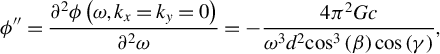 $$\begin{align}{\phi}^{\prime \prime}=\frac{\partial^2\phi \left(\omega, {k}_x={k}_y=0\right)}{\partial^2\omega}=-\frac{4{\pi}^2 Gc}{\omega^3{d}^2{\mathit{\cos}}^3\left(\beta \right)\cos \left(\gamma \right)},\end{align}$$
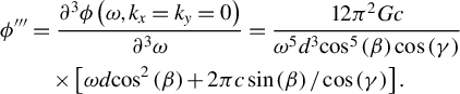 $$\begin{align}{\phi}^{\prime \prime \prime}&=\frac{\partial^3\phi \left(\omega, {k}_x={k}_y=0\right)}{\partial^3\omega}=\frac{12{\pi}^2 Gc}{\omega^5{d}^3{\mathit{\cos}}^5\left(\beta \right)\cos \left(\gamma \right)}\nonumber\\& \quad \times \left[\omega d{\mathit{\cos}}^2\left(\beta \right)+2\pi c\sin\left(\beta \right)/\cos \left(\gamma \right)\right].\end{align}$$
Here, $c$
is the speed of light in vacuum,
$c$
is the speed of light in vacuum, $\alpha$
is the incident angle,
$\alpha$
is the incident angle, $\gamma$
is the out-of-plane incident angle,
$\gamma$
is the out-of-plane incident angle, $\beta$
is the diffraction angle defined by grating formula
$\beta$
is the diffraction angle defined by grating formula $d\left[\sin \left(\alpha \right)+\sin \left(\beta \right)\right]=\lambda /\cos \left(\gamma \right)$
,
$d\left[\sin \left(\alpha \right)+\sin \left(\beta \right)\right]=\lambda /\cos \left(\gamma \right)$
, $G$
is the grating perpendicular distance and
$G$
is the grating perpendicular distance and $d$
is the grating period. Through Equations (1)–(4), it is easy to simulate compressed pulse temporal and spatial characteristics of the DSGC.
$d$
is the grating period. Through Equations (1)–(4), it is easy to simulate compressed pulse temporal and spatial characteristics of the DSGC.
2.2 Beam smoothing
To evaluate the smoothing effect of compressors, the laser spatial intensity modulation (LSIM) values of input and output spots are calculated, which are generally defined as the ratio between the local maximum intensity to the average beam intensity of the main area.
The smoothing simulation using the YSGC was conducted by introducing Gaussian type hot spots in a 400 mm × 400 mm 10th-order super-Gaussian light spot, with 14 fs Fourier transform limit (FTL) pulse duration. Based on established PW facility parameters[ Reference Gan, Yu, Wang, Liu, Xu, Li, Li, Yu, Wang, Liu, Chen, Peng, Xu, Yao, Zhang, Chen, Tang, Wang, Yin, Liang, Leng, Li, Xu, Yamanouchi, Midorikawa and Roso8, Reference Li, Gan, Yu, Wang, Liu, Guo, Xu, Xu, Hang, Xu, Wang, Huang, Cao, Yao, Zhang, Chen, Tang, Li, Liu, Li, He, Yin, Liang, Leng, Li and Xu32– Reference Li, Leng and Li34], hot spot radii were systematically varied from 1 to 10 mm with spatial alignment along the X-axis. Since temporal characteristics remained consistent across spatial configurations, our analysis focused specifically on spatial fluctuation evolution through the compressor. As Figure 2(a) shows, the LSIMs of output pulses decrease quickly with the increase of the out-of-plane angle from 0° to 20°, with different speeds for different radii. As expected, smaller hot spots exhibited greater LSIM reduction magnitudes, as quantified by ΔLSIM = max(LSIM)–min(LSIM) in the embedded plot. Specifically, 1 mm hot spots showed LSIM reduction from 2.0 to 1.03, while their 10 mm counterparts decreased from 2.0 to 1.18.
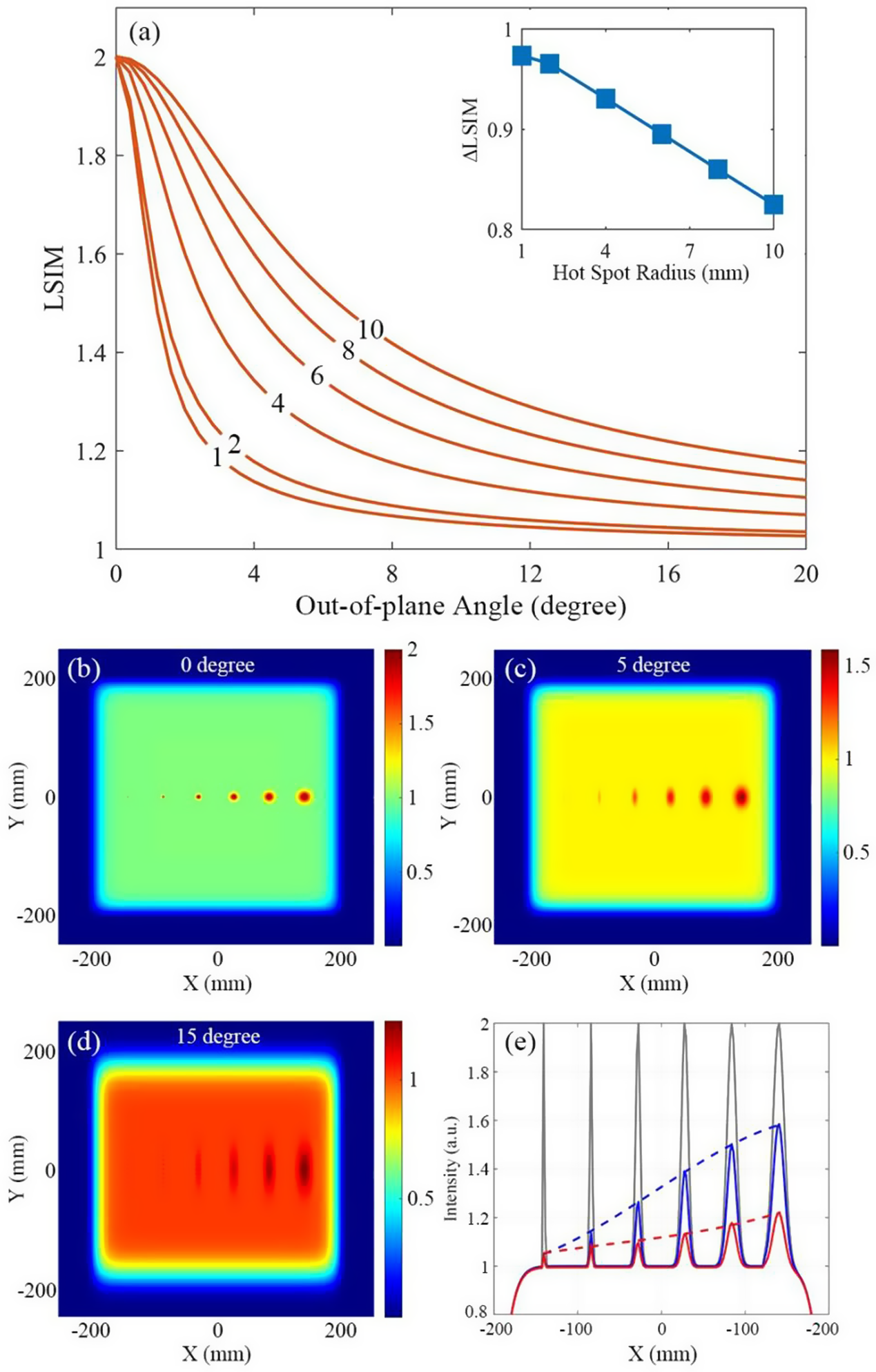
Figure 2 The relationships of LSIM and out-of-plane angle with different hot spot radii are shown in (a). The inset figure illustrates the relation between the ΔLSIM and hot spot radius. (b)–(d) The spatial intensity distributions of the output pulse from the YSGC with out-of-plane angles γ = 0°, 5° and 15°. The intensity along the X direction at Y = 0 mm is shown in (e), in which black, blue and red lines represent γ = 0°, 5° and 15°, respectively.
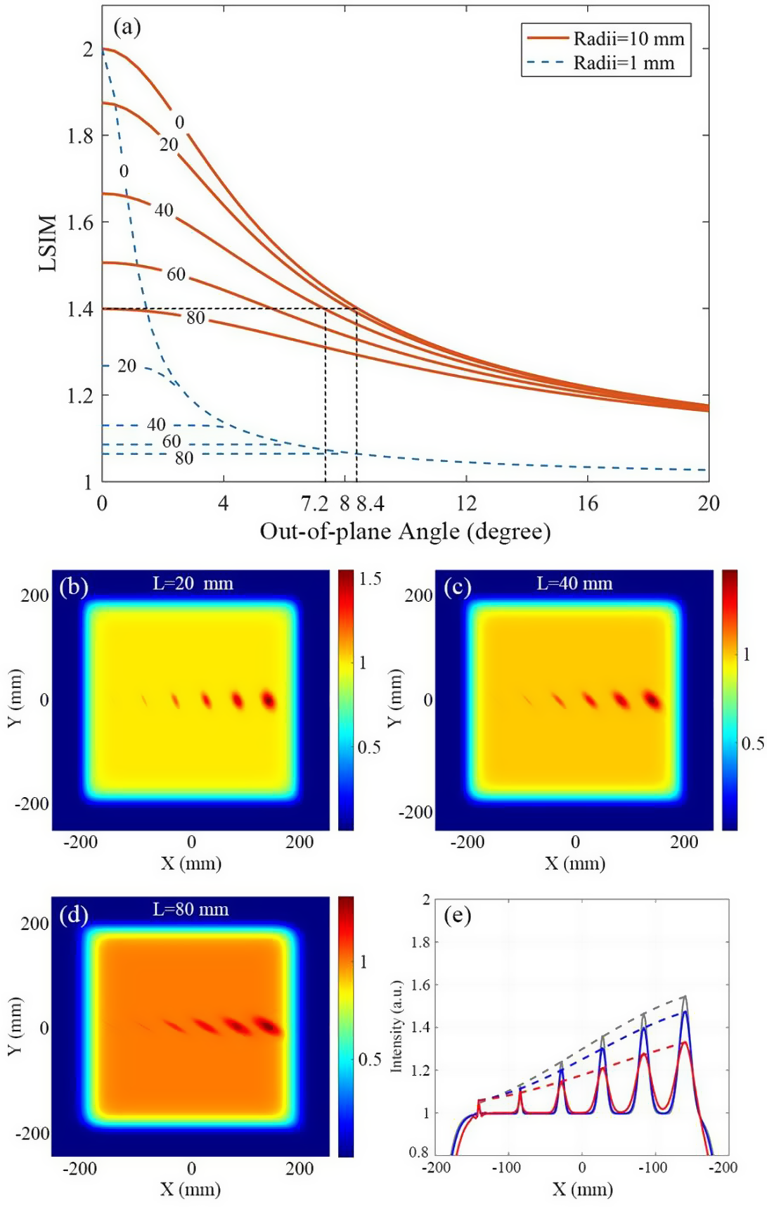
Figure 3 (a) The relationships between LSIM and out-of-plane angles with different grating pair distance variations from 0 to 80 mm. The red full lines represent hot spot radius of 10 mm and blue dashed lines represent 1 mm. (b)–(d) The spatial intensity distributions of the output pulse from the DSGC with grating distance variations L = 20, 40 and 80 mm, when γ = 5°. The intensities along the X direction in Y = 0 mm are shown in (e), in which black, blue and red lines represent L = 20, 40 and 80 mm, respectively.
Detailed spatial intensity evolutions are shown in Figures 2(b)–2(d), demonstrating significant smoothing effects: hot spot structures become markedly suppressed at γ = 5° and reach near-minimal LSIM values at γ = 15°. Figure 2(e) displays corresponding X-axis intensity profiles (Y = 0 mm) for comparative analysis. Although LSIM reduction continues beyond γ > 20°, spectral diffraction efficiency experiences significant degradation[ Reference Han, Li, Zhang, Kong, Cao, Jin, Leng, Li and Shao27], which might influence the output temporal characteristics. To achieve optimal smoothing while preserving temporal characteristics, γ = 15° was maintained throughout subsequent experimental and numerical investigations.
The DSGC configuration is achieved by implementing additional spatial dispersion along the X-axis. Figure 3(a) illustrates the LSIM variation profiles as functions of out-of-plane angle (γ) and grating pair distance variation (L)[ Reference Shen, Du, Liang, Wang, Liu and Li19]. For 1 mm radius hotspots in the AFGC (γ = 0°), LSIM reaches 1.06 at L = 80 mm, approaching the minimum LSIM of 1.03 achieved through pure angular dispersion (γ = 20°, L = 0 mm). This comparison reveals transverse spatial dispersion’s significant smoothing contribution at low γ values. For radii of 10 mm, the LSIM is reduced to 1.40 by the AFGC with 80 mm grating distance, while for the YSGC, the same LSIM value is achieved with just an 8.4° out-of-plane angle, showing greater dispersion ability. Furthermore, if employing the DSGC, only a 40 mm grating distance and a 7.2° out-of-plane angle are introduced to obtain 1.40 LSIM, avoiding spectral shearing caused by grating shifting and diffraction efficiency decreasing caused by a large out-of-plane angle. Under the most effective circumstances, the DSGC with L = 80 mm and γ = 20° can decrease LSIM to 1.16 for a 10-mm-radius hot spot.
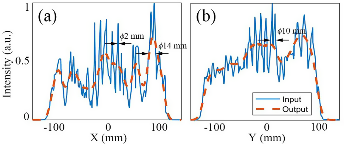
Figure 4 (a), (b) Intensity distributions before and after the DSGC in the X and Y directions, respectively. The blue solid lines refer to the intensities before the DSGC, while the red dashed lines refer to the intensities after the DSGC. The input intensity distributions along the X and Y directions are from Figure 3 in Ref. [Reference Li, Gan, Yu, Wang, Liu, Guo, Xu, Xu, Hang, Xu, Wang, Huang, Cao, Yao, Zhang, Chen, Tang, Li, Liu, Li, He, Yin, Liang, Leng, Li and Xu32].
Maintaining a fixed γ = 5°, transverse spatial dispersion becomes essential for further LSIM reduction. Figures 3(b)–3(d) illustrate the spatial intensity distributions from the DSGC with varying L when γ = 5°. It is easy to note that for larger hot spot radii, the effect of L is more important. When the radius is 1 mm, 80 mm grating distance contributes 0.05 LSIM decline compared to the YSGC in Figure 2(c). However, when the radius is 10 mm, it brings a 0.25 LSIM decline. The intensities along the X direction at Y = 0 mm of different L values are illustrated in Figures 3(e) and 2(e).
Simulation results demonstrate two key advantages of the DSGC. Firstly, because the longitudinal spatial dispersion is introduced by the out-of-plane angle, the dispersion quality can be considerable for no light path blocking. Secondly, the combination of transverse and longitudinal spatial dispersion has a superior smoothing effect on the single YSGC or AFGC. Practically, in applications, the spatial intensity distributions are more complicated, so in the next section a proof-of-concept experiment has been conducted to further verify the practicality and effectiveness of the DSGC.
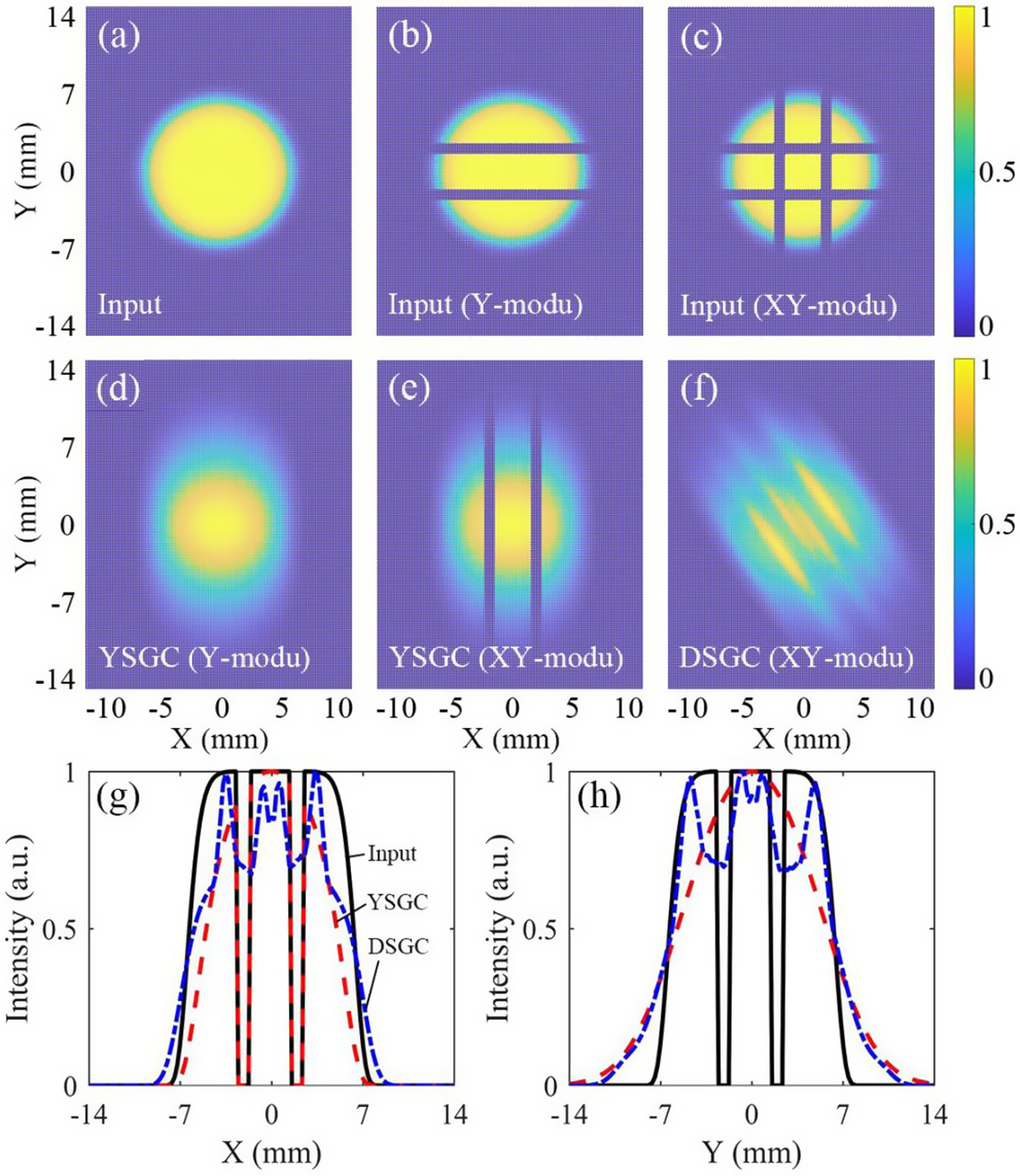
Figure 5 Numerical simulation results of light spots from the YSGC or DSGC. (a) Uncompressed input spot without modulation. (b) Input spot with longitudinal modulation, and (d) corresponding output spot from the YSGC. (c) Input pulse with longitudinal and transverse modulation. (e), (f) Corresponding output spots from the YSGC and DSGC, respectively. (g), (h) Intensity distributions of (c), (e) and (f) along the X and Y directions, respectively.
With the same simulation program above, the DSGC’s smoothing effect for a real high-power laser facility[ Reference Li, Gan, Yu, Wang, Liu, Guo, Xu, Xu, Hang, Xu, Wang, Huang, Cao, Yao, Zhang, Chen, Tang, Li, Liu, Li, He, Yin, Liang, Leng, Li and Xu32] is verified. The pulse diameter after amplifier is 235 mm, with 21 fs duration and 800 nm central wavelength. The near-field intensity distribution is as shown in Figure 3 of Ref. [Reference Li, Gan, Yu, Wang, Liu, Guo, Xu, Xu, Hang, Xu, Wang, Huang, Cao, Yao, Zhang, Chen, Tang, Li, Liu, Li, He, Yin, Liang, Leng, Li and Xu32]. With 15° out-of-plane angle and 80 mm grating distance variation, the intensity modulations in the X and Y directions were extremely smoothed, as Figures 4(a) and 4(b) show. The diameters of hot spots signed by arrows are from 2 to 14 mm, which are in accordance with the simulation above. To quantificationally evaluate the spatial intensity modulation degree, the intensity peak to average (PTA) values of input and output spots are calculated. The formula of the PTA is as follows:
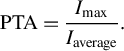 $$\begin{align}\mathrm{PTA}=\frac{I_{\mathrm{max}}}{I_{\mathrm{average}}}.\end{align}$$
The PTA values in the X and Y directions are represented by PTA x and PTA y , respectively. After the smoothing of the DSGC, PTA x decreased from 2.31 to 1.82 (21.2% reduction), while PTA y decreased from 1.87 to 1.38 (26.2% reduction), demonstrating a theoretical energy boost by (2.31/1.82) × (1.87/1.38) = 1.72 times. Note that in this part of the simulation, the smoothing effects of the two directions are considered separately, so it is reasonable to calculate their contribution to energy boost by multiplying them. If considering the oblique incidence of the light spot on the grating caused by the out-of-plane angle, the output energy can be further increased.
For further testing the smoothing effect of the YSGC and DSGC, combining with the Fourier diffraction formula, simulation of a spot smoothing experiment was conducted. The simulation results are illustrated in Figure 5. For longitudinal modulation in Figure 5(b), the YSGC can smooth it completely with a 15° out-of-plane angle, as shown in Figure 5(d). However, for transverse modulation, the YSGC has little effect, while the DSGC eliminates the modulations in the two directions simultaneously, for which smoothed light spots are shown in Figures 5(e) and 5(f). Through illustrating the intensity distribution at Y = 0 or X = 0, it reveals that the gaps in the X or Y direction are compensated by frequency components in other parts after the DSGC, as depicted in Figures 5(g) and 5(h). The minimum normalized intensity was increased from 0 to 0.68 by the DSGC, demonstrating a powerful ability of redistributing energy in space.
3 Experimental results
3.1 Pulse compression
Pulse compression capabilities were systematically evaluated using γ = 15° (YSGC) and L = 60 mm (DSGC) configurations with a Ti:sapphire oscillator uncompressed pulse (123.7 ps full width at half maximum (FWHM) duration, 14 mm beam diameter, 49° grating incidence). The pulse temporal profiles were measured by a home-made transient grating-based self-reference spectral interferometer (TG-SRSI), for which energies are normalized, as Figure 6 shows. The compressed pulse durations after the three types of compressors are 43.0, 43.1 and 43.6 fs, respectively, which are close to the FTL duration of 35.5 fs, calculated by the spectrum of the output pulse. Due to the high-order dispersion introduced by the stretcher and amplifier, even the FGC cannot compress the pulse to the FTL duration. The compression efficiency of the DSGC decreased by 10% to 76%, compared to the FGC’s 84%, which is consistent with the data measured by Han et al. [ Reference Han, Li, Zhang, Kong, Cao, Jin, Leng, Li and Shao27]. Furthermore, intensity profile analysis reveals that pulse wing variations account for observed peak intensity discrepancies between configurations.
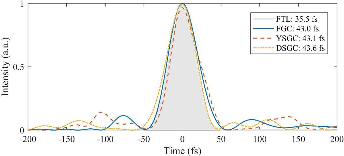
Figure 6 The gray area represents the FTL pulse profile retrieved by the spectrum. The blue solid line, red dashed line and yellow chain line represent pulse temporal profiles compressed by the FGC, YSGC and DSGC, respectively.
The pulse duration discrepancies among the FGC, YSGC and DSGC configurations result from spatially nonuniform frequency distributions inducing tiny (<2%) temporal broadening in near-field propagation. On the other hand, as was shown in Refs. [Reference Khazanov20,Reference Khazanov23], the introduction of spatial dispersion has no impact on far-field intensity, which is a primary goal for most applications.
3.2 Beam smoothing
A proof-of-concept experiment was done by adding 1-mm-wide paper tapes on a diaphragm for pre-compression spatial modulation. Figure 7 demonstrates remarkable consistency between experimental results and numerical simulations: Figure 7(a) shows the non-modulated beam profile with negligible diffraction rings from the diaphragm aperture, Figure 7(b) displays the Y-axis longitudinal modulation and Figure 7(c) presents combined longitudinal–transverse modulation. The charge-coupled device (CCD) detection plane, positioned 500 mm from the modulation diaphragm (matching the first grating-to-diaphragm distance), recorded the beam profiles. Therefore, the modulated spot shows some diffraction characteristics. Note that similar experiments were made in Ref. [Reference Kiselev, Kochetkov, Yakovlev and Khazanov31] where horizontal smoothing was provided not by different grating distances but by different incident angles in the diffraction plane.
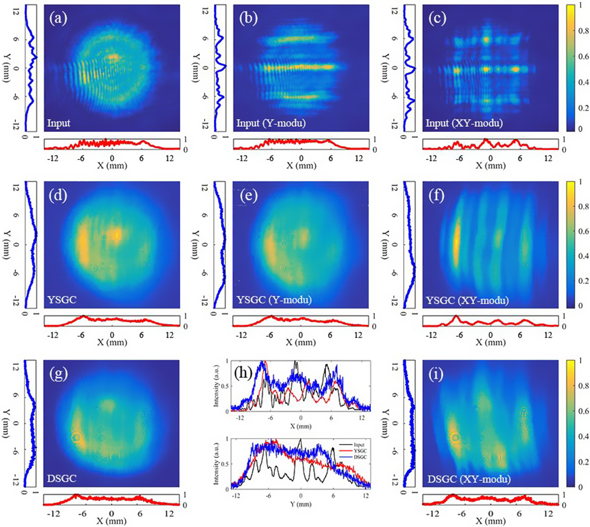
Figure 7 The spatial intensity distributions of input pulses without modulation (a), with longitudinal modulation (b) and with longitudinal and transverse modulation (c). (d)–(f) Corresponding spatial intensity distributions of output pulses from the YSGC. (g), (i) Output pulses of (a) and (c) from the DSGC. (h) Intensity distribution comparison along the X or Y direction of (c), (f) and (i).
Firstly, we separately analyze the spatial intensity distribution change before and after the YSGC. Not only the PTA in the X or Y direction (represented by PTA x or PTA y , respectively), but also the PTA of the whole spot (represented by PTAall) is used in evaluation. Figures 7(d)–7(f) illustrate the output spot intensity distributions from the YSGC, corresponding to the input spots from Figures 7(a)–7(c), respectively. With the smoothing effect of the YSGC, the PTA x of the spot without modulation decreased from 1.63 to 1.61 (1.2% reduction) after compression, PTA y decreased from 1.86 to 1.40 (24.7% reduction) and PTAall decreased from 5.21 to 3.16 (39.3% reduction). The obvious PTA decline in the whole spot after the YSGC demonstrates that the output energy can be increased by 1.65 times considering the damage threshold of the grating. For the input pulse with longitudinal modulation, the smoothness of the YSGC in the Y direction is more conspicuous. As Figures 7(b) and 7(e) show, PTA y decreased from 2.59 to 1.29 (50.2% reduction), corresponding to output energy increasing by 2.01 times. In addition, PTAall decreased from 6.09 to 3.32 (45.5% reduction), corresponding to output energy increasing by 1.83 times. A more comparative situation was considered with a longitudinal and transverse modulated input pulse, for which input and output spots are shown in Figures 7(c) and 7(f). It is evident that the hot spots in Figure 7(c) were smoothed to strips in the Y direction by the YSGC, but in the X direction the PTA x did not decrease. The detailed PTA values of all the spots are listed in Table 1.
Although the YSGC has a remarkable smoothing effect in the longitudinal direction, the hot spots in the practical output spot are irregular, such as those shown in Figure 7(c). Modulation in the transverse dimension cannot be eliminated effectively by the YSGC. Analogously, it is the same for the AFGC. Therefore, it is natural to simultaneously introduce out-of-plane angle and grating pair distance difference in the FGC to smooth the spot in two dimensions – that is, the DSGC. It was proposed in Ref. [Reference Khazanov20] and implemented in a proof-of-principle experiment in Ref. [Reference Kiselev, Kochetkov, Yakovlev and Khazanov31] where horizontal smoothing was provided not by different grating distances but rather by different incident angles in the diffraction plane. We introduced a 60 mm perpendicular distance change of two grating pairs in the YSGC, with which one can obtain sufficient transverse spatial dispersion while avoiding spectral shearing.
Table 1 PTA values of measured spots.
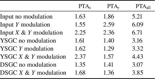
For the input spot without modulation, the DSGC shows a better smoothing ability in the X direction compared to the YSGC, as Figure 7(g) illustrates. For the input spot with longitudinal (Y) and transverse (X) modulation, the DSGC has a more prominent smoothing effect, no matter whether in the X or Y direction, as Figure 7(i) shows. As for the input spot with longitudinal modulation, its output spot from the DSGC is similar to that shown in Figure 7(g), and is not shown separately. An obvious contrast can be seen from PTA values. When PTA x decreased from 2.25 to 1.68 (25.3% reduction), PTA y decreased from 2.36 to 1.36 (42.4% reduction), which is much lower than the value for the YSGC. For PTAall, it decreased by 1.74 times, which means a 0.74 times output energy increase achieved by the DSGC. For the YSGC, this value is 0.51. More visualized intensity distributions along the X and Y directions of Figures 7(c), 7(f) and 7(i) are depicted in Figure 7(h). The transverse and longitudinal spatial modulations were eliminated step-by-step by introducing corresponding spatial dispersion.
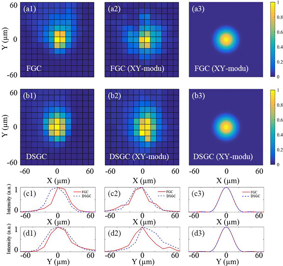
Figure 8 The far fields of output light spot from the FGC and DSGC. From left to right, the first to third columns are the input pulses without modulation, with longitudinal and transverse modulation and corresponding simulation results. Lines 1–3 are far fields of the FGC and DSGC and intensity distributions along the X or Y direction.
3.3 Focal spots
Practical applications prioritize far-field beam quality due to its direct correlation with focal intensity maxima, as demonstrated through experimental measurements using a 300 mm focal-length lens and 11 μm/pixel CCD resolution (Figure 8). The FGC exhibited comparable FWHM dimensions (22 μm X/33 μm Y) for both modulated and unmodulated inputs, aligning with simulated 24 μm predictions. For the DSGC, the FWHM increased to 33 μm in the X direction and 44 μm in the Y direction for both with and without modulation input spots, due to the spatial dispersion. Although the focal spots compressed by the DSGC present a little broadening on the spatial scale, the overall intensity distribution is compact and uniform, demonstrating a high focal quality. Once again we emphasize that, as was shown in Refs. [Reference Khazanov20,Reference Khazanov23], far-field intensity is the same for any type of compressor – AFGC, YSGC and DSGC.
4 Discussion and conclusion
The compressor, comprising gratings with limited damage threshold and size, is the main factor limiting high-peak-power laser output currently. Therefore, improving grating area utilization and reducing spot spatial intensity modulation are two important approaches promoting output power under the limited grating size.
The recent multistep pulse compressor (MPC) was proposed as an efficient path to achieving hundreds-of-PW lasers by reducing spot spatial intensity modulation only[ Reference Liu, Shen, Du and Li35]. Further, the DSGC can be a key step to replace the AFGC in MPCs, without adding any additional components. Also, full-aperture compressors[ Reference Trentelman, Ross and Danson36– Reference Vyatkin and Khazanov38] may be upgraded by this double-axis smoothing. Different from the in-plane compressor, the three-dimensional structure of the DSGC allows the grating area to be fully utilized without spectral shearing[ Reference Kalinchenko, Vyhlidka, Kramer, Lerer and Rus25, Reference Smith, Erdogan and Erdogan28]. In particular, due to the introduction of out-of-plane angles, the intensity of the spot can be dispersed in the longitudinal direction of the grating. Meanwhile, the double-smoothing function of the DSGC further improves the tolerance of spot intensity, which is significantly superior to those of the YSGC and AFGC according to the simulations and principle-verification experiments. Moreover, the compressed pulse from the DSGC can be improved further by post-compression[ Reference Chen, Liang, Xu, Shen, Wang, Liu and Li39, Reference Khazanov, Mironov and Mourou40].
In summary, through simulation and an experiment on a home-made FGC system, the temporal compression, focus ability and spatial smoothing abilities of the DSGC were verified and it was demonstrated that the DSGC has a superior smoothing effect compared with the YSGC or AFGC. The simulation considering the single hot spot verified that by introducing an appropriate out-of-plane angle and grating pair distance difference, LSIM can be decreased from 2.0 to 1.16. Simulation results of a practical amplified spot in a 10 PW facility proved its smoothing ability once again. Later a smoothing simulation and a corresponding pulse compression experiment employing the DSGC confirmed the DSGC’s smoothing effect by calculating the PTA of near-field spots. In addition, the temporal and far-field characteristics of the DSGC were not significantly different from those of traditional TCs.
Overall, based on its practicality, effectiveness and simplicity, the DSGC has certain application potential in high-power laser facilities.
Acknowledgements
This work was supported by the Shanghai Municipal Natural Science Foundation (Grant No. 20ZR1464500), the National Natural Science Foundation of China (NSFC) (Grant Nos. 61905257 and U1930115), the Shanghai Municipal Science and Technology Major Project (Grant No. 2017SHZDZX02) and the Ministry of Science and Higher Education of the Russian Federation (Project No. FFUF-2024-0038).
Author contributions
J. L., E. A. K., X. S. and R. C. conceived the idea. R. C. performed the simulations. R. C., W. L., S. D. and Y. X. performed the experiments. J. L., R. C., X. S. and P. W. analyzed the data. R. C. and J. L. prepared the manuscript and discussed it with all authors. J. L., E. A. K., Z. L. and R. L. supervised the project.


 Open access