


1. Introduction
The large bandwidth available in the millimeter-wave (mm-wave) band can be used for high capacity and high data-rate applications in 5G. The n257 and n258 5G New Radio bands are defined at the lower end of the mm-wave spectrum between 24.25 and 29.50 GHz [1]. The higher propagation loss in the mm-wave band compared to the 4G frequency range below 6 GHz requires smaller cell sizes for 5G mm-wave. Providing complete coverage in Urban Macro and Urban Micro cells with inter-site distances of typically 500 and 200 m [2, 3], respectively, is very challenging at mm-wave. Challenges of 5G mm-wave communication include high propagation losses and shadowing [Reference Rangan, Rappaport and Erkip4]. Many mm-wave channel measurements are required for accurate channel characterization and modeling.
Wideband mm-wave channel measurements are often performed with expensive channel sounders. Popular channel sounders are the wideband-correlation [Reference Papazian, Gentile, Remley, Senic and Golmie5, Reference Muller, Hafner, Dupleich, Luo, Schulz, Herrmann, Schneider, Thoma, Lu and Wang6], sliding-correlation [Reference Rappaport, MacCartney, Samimi and Sun7, Reference Kwon, Kim and Chong8] and Vector Network Analyzer (VNA) [Reference Yang, Smulders and Herben9–Reference Lei, Zhang, Lei and Du11] based channel sounders. Wideband correlation channel sounders are capable of fast untethered channel measurements, but require high-speed analog-to-digital converters. Sliding-correlation channel sounders alleviate this requirement at the cost of a longer measurement time. VNAs require even longer measurement times, but have a simpler system design and require less additional hardware. VNAs require a wired connection between the transmitter and receiver and are thus limited to short-range measurements.
An untethered mm-wave measurement setup for narrowband path loss (PL) and angle-of-arrival (AOA) measurements, which can be composed with hardware that is either low-cost or ubiquitous in most radio-frequency (RF) laboratories, is presented in this paper. This setup is a cost-effective narrowband alternative to conventional channel sounders for PL and AOA measurements. An algorithm is developed to improve the measurement accuracy and limit the measurement time of the setup. An uncertainty analysis is performed to provide insight into the trade-offs between measurement time and accuracy and the combined standard uncertainty is estimated. The measurement setup is designed for evaluation of the 24 GHz band, but the presented setup can also be used for measurements in other frequency bands. This is only limited by the frequency range of the hardware. The algorithm and uncertainty analysis can also be applied in other frequency bands, but system parameters and settings might have to be adjusted and uncertainties will vary.
5G mm-wave early deployment targets high capacity applications, like stadiums and open squares. The coverage range of a base station at an open square might be extended to non-line-of-sight (NLOS) areas by smart use of building reflections. Previous research shows that building materials like tinted glass, metal and concrete can provide low-loss mm-wave reflections [Reference Zhao, Mayzus, Sun, Samimi, Schulz, Azar, Wang, Wong, Gutierrez and Rappaport12, Reference Violette, Espeland, DeBolt and Schwering13]. The developed measurement setup is used to measure the PL and AOA in a NLOS area, where two buildings could provide low-loss paths via specular reflections.
The novelties presented in this work include an algorithm for improved measurement accuracy and reduced measurement time, an uncertainty analysis of a narrowband measurement setup and an analysis of mm-wave specular building reflections. The remaining of this paper is organized as follows. The measurement setup and algorithm are discussed in section “Cost-effective mm-wave measurement setup for narrowband PL and AOA measurements”. The uncertainty analysis of the measurement setup is presented in section “Uncertainty analysis”. The measurement scenario and results of specular building reflections are discussed in sections “Measurement scenario” and “Measurement results”, respectively. This paper is concluded in section “Conclusion”. This work is an extended version of a paper, which was presented at the European Conference on Antennas and Propagation 2020 (EuCAP 2020) and was published in its Proceedings [Reference Schulpen, Bronckers, Smolders and Johannsen14].
2. Cost-effective mm-wave measurement setup for narrowband PL and AOA measurements
2.1 Hardware
A block diagram of the measurement system is depicted in Fig. 1. At the transmitter (Tx), a 0 dBm continuous-wave (CW) signal is sequentially generated at 24.000, 24.125, and 24.250 GHz by an HP8350B sweep oscillator (SO). This signal is amplified by a 20 dB power amplifier (PA) [15]. The signal power is measured with a hand-held FieldFox N9918A spectrum analyzer (SA) at the receiver (Rx) after it is amplified by a 23 dB low-noise amplifier (LNA) [16]. The Tx and Rx antennas are identical 17 dBi standard gain horn antennas with a half-power beamwidth (HPBW) of 24.2° in the H-plane and 24.6° in the E-plane [17]. A vertical antenna polarization is used as default setting.

Fig. 1. Block diagram of the measurement setup.
The Rx antenna is rotated 360° in 9° steps in the horizontal ϕ-plane by a low-cost motorized rotation platform, which is depicted in Fig. 2. This rotation platform is 3D-printed using the Fused Deposition Modeling (FDM) process. The rotation is accomplished by stepper motors with drivers, which are controlled via an Arduino micro-controller. The position of the rotation platform with respect to the cart is determined using a Hall sensor. The orientation of the cart with respect to True North is determined with a compass and a compensation for the declination angle is applied. The rotation platform is initialized at each measurement location to align the Rx pointing angle ϕ = 0° to True North.

Fig. 2. Picture of the measurement equipment.
The core components of the measurement setup are the SO and SA. The purpose of the amplifiers is to increase the maximum measurable PL. The SO is well suited for the transmission of CW signals with the option to sequentially transmit several discrete frequencies. The SA is designed for the analysis of the RF spectrum, but it can also be used for power measurements. The advantage of a SA over a broadband power sensor is its larger dynamic range, higher sensitivity, and suppression of out-of band interference at the cost of a reduced amplitude accuracy [Reference Small18]. The peak detector setting is used during the measurements for the detection of the CW signals. The amplitude accuracy of the SA can be improved by optimization of its settings, often at the cost of an increased measurement time.
The SA and LNA are equipped with batteries to enable untethered wireless channel measurements. A challenge for untethered PL measurements is the relative frequency drift between the SO and SA. This drift can cause the received signal to fall outside the measured frequency span of the SA. Measurement of a large frequency span with many points could eliminate this issue, but at the cost of an increased measurement time. The choice of resolution bandwidth (RBW) of the SA is a trade-off between dynamic range and measurement time. The relative frequency drift affects the minimum possible RBW, because the signal may not drift outside the measured RBW during its measurement.
2.2 Software (algorithm)
An algorithm is developed to enable accurate and fast PL measurements on a SA. The algorithm enables measurements with a small frequency span and small RBW, where the measurement time is greatly reduced by the small frequency span compared to conventional SA measurements. Multiple snapshots can be measured to improve the measurement accuracy.
A flow chart of the algorithm is depicted in Fig. 3. The algorithm consists of two stages: an initialization stage and a measurement stage. The main parameters of the SA are its center frequency f c, frequency span f span, number of frequency points N f, and RBW. The parameters for both stages are given in Table 1. The purpose of the initialization stage is to detect the frequency f p at which the peak signal is detected by the SA. The measurement time of the single snapshot taken in this stage is relatively long due to the large 8 MHz frequency span that is required to always detect the signal at the start of the measurement when the relative drift is not known accurately. f p is used as center frequency for the first snapshot of the measurement stage. In the measurement stage, the frequency span is reduced to 25 kHz, which reduces the measurement time while remaining wide enough to capture the signal. N s snapshots are taken for each measurement to improve the measured power accuracy. After each snapshot, f c is updated to the f p of the previous snapshot to keep the received signal within f span. After N s snapshots are taken, the logarithmic mean of the peak power of the snapshots is calculated as P meas.

Fig. 3. Flow chart of the measurement algorithm.
Table 1. Parameters of the initialization and measurement stage of the measurement algorithm with the two options O1 and O2 for the measurement stage

This algorithm is repeated for all carrier frequencies. Synchronization of the SO and SA is accomplished by synchronizing the Tx and Rx sweeps with the system time of the Tx and Rx systems, respectively. Guard intervals of 1 s are used to maintain synchronization in case of relative clock drift during a measurement campaign.
2.3 Measurement settings and parameters
Two measurement setting options are considered: option 1 (O1) with RBW = 1 kHz and N f = 2001 and option 2 (O2) with RBW = 5 kHz and N f = 401. The impact of N f on the measurement time is small in case of the used FFT mode and small f span on the SA. The 1 kHz RBW is the smallest RBW that can be used without severe measurement impairments, which are due to the relative frequency drift being too large compared to the measurement time of one frequency bin. Accuracy of measurements with a 5 kHz RBW is less affected by the drift, but is more affected by noise. These measurement settings are compared in the uncertainty analysis in section “Uncertainty analysis”. The impact of N s on the measurement accuracy is also investigated there.
The PL in dB can be calculated as

where P cal(f) is a calibration term in dBm and

where P meas(f, ϕ, n) is the measured power in dBm at frequency f, Rx pointing angle ϕ and snapshot n, and N s(f, ϕ) is the number of snapshots. The measurement system is calibrated via an over-the-air (OTA) calibration as described in [Reference Schulpen, Konstantinou, Rommel, Johannsen, Tafur Monroy and Smolders19], which provides calibration term P cal(f). The mean PL as function of ϕ can be calculated as

where 〈 · 〉f denotes the mean over frequency. The antenna pattern is not de-embedded from the measurements, hence $\overline {{\rm PL}}( \phi )$ should be evaluated at its minimum. The minimum PL is defined as

where ϕ min denotes the Rx pointing angle at which the mean PL over frequency is minimum.
3. Uncertainty analysis
The uncertainty analysis of the measurement setup focuses on the stability of $P^{av}_{meas}$ and P meas, because constant offsets are compensated for by P cal(f) in (1). Measurement setting options O1 and O2 are compared at 24.25 GHz. This uncertainty analysis includes a noise analysis, general system impairments, amplifier linearity, and antenna misalignment. The chosen measurement settings for the measurement campaign and the corresponding combined uncertainty are discussed at the end of this section.
3.1 Noise analysis
Noise can severely impact the measurement accuracy and stability at low received power levels. The goals of this noise analysis are to determine the relationship between receiver noise and the uncertainty of P meas, and to determine how averaging of multiple snapshots improves the uncertainty of $P^{av}_{meas}$ . The first step in the noise analysis is to model the receiver noise. It is assumed that the receiver noise is additive white Gaussian noise (AWGN). The noise voltage detected at the envelope detector within the SA then exhibits a Rayleigh distribution [20]. The probability density function (PDF) of this Rayleigh distribution is defined as

where σ is the Rayleigh parameter and x the envelope voltage in mV. The measured receiver noise power P noise in dBm can be written as the transformed random variable

The PDF of Y can be calculated via the change-of-variable technique [Reference Hogg, Tanis and Zimmerman21] as

The noise of the Rx including LNA is measured in order to verify (7) for a RBW of 1 kHz (O1) and 5 kHz (O2). The sample detector mode of the SA is used with f span = 5 MHz and N f = 501. These different measurement settings are required to accurately determine the noise distribution for O1 and O2 in the presence of a CW signal. In total, 1377750 noise floor samples are measured for each option and the corresponding probability distributions are depicted in Fig. 4. The fit of f Y(y, σ) to the measured noise is plotted as a solid line. The calculated PDFs fit the measurement data well, which validates the AWGN assumption. The estimated Rayleigh parameters are σ = 2.4×10⁻⁴ for O1 and σ = 5.3×10⁻⁴ for O2. The noise floor is 7 dB higher in case of O2, which is due to its five times larger RBW.

Fig. 4. Probability distribution of receiver noise power P noise for O1 and O2. The fit of the noise model to the measurement data is plotted by a solid line.
The next step is to include the CW signal and create the signal plus noise model

where v signal is the received RMS signal voltage, v noise is the Rayleigh distributed noise random variable, and ϕ noise is the uniformly distributed phase of the noise relative to the signal phase. The measured power can then be calculated as

A back-to-back measurement of the complete setup with P meas ≈ -60.5 dBm on average is performed for O1 and O2 to validate the signal plus noise model. The measurement settings in Table 1 are used and 18800 samples are measured for O1 and O2 each. The theoretical model in (8) and (9) uses 10 million samples to obtain a probability distribution that approximates the PDF. The Rayleigh parameters obtained from (7) for O1 and O2 are used in the signal plus noise model. The probability distribution of the measurements is compared to this model in Fig. 5. The model shows a good match with the measurement data for both O1 and O2. The higher noise power of O2 results in a larger spread in P meas.

Fig. 5. Comparison of the signal plus noise model with measurement data for O1 and O2.
The final step in the noise analysis is to investigate the effect of averaging on the uncertainty of $P^{av}_{meas}$ . The signal plus noise model in (8) and (9) is used in a Monte Carlo simulation to obtain one million instances of N s snapshots of P meas. These snapshots are averaged to obtain $P^{av}_{meas}$
 for each instance. The error can be defined as

where P signal is the theoretical received signal power in dBm at the input of the SA. A Monte Carlo simulation is run for O1 and O2, with P signal ranging from − 75 to −30 dBm in 5 dB steps and for an N s of 1, 10, and 100. Figure 6 depicts the probability distribution of ε for O1 with P signal = −75 dBm and N s = 10. The 95.45% confidence interval is calculated as

where ν is the confidence limit. The − ν and ν bounds in Fig. 6 show that 95.45% of the averaged measurements have an absolute error of less than 1.1 dB. Confidence limit ν is used as a measure for the uncertainty due to receiver noise. The probability distribution of ε approximates a normal distribution N ~ (0, σ N) when P signal ≫ P noise with ν equal to 2σ N.

Fig. 6. Probability distribution of ε for O1 with P signal = −75 dBm and N s = 10.
Figure 7 depicts ν as a function of P signal for O1 and O2 with N s equal to 1, 10, and 100. ν is large for P signal close to the noise floor, but can be decreased by taking more snapshots. ν decreases for increasing P signal and is less than 0.1 dB for P signal > −35 dBm.

Fig. 7. Confidence limit ν of the error due to receiver noise as function of P signal for O1 and O2 and various N s.
3.2 General system impairments
The general system impairments are defined as the non-separable impairments that affect the stability of P meas. These include temperature drift and the relative frequency drift between the SO and SA. The general system impairments are estimated in a temperature-controlled lab with limited temperature variation. Larger variations in the environmental temperature during measurement campaigns could increase the uncertainty, but this is regarded as future research.
The general system impairments are estimated by measuring a back-to-back measurement of the setup with P signal ≈ −10 dBm. The confidence limit ν for noise variation at P signal = −10 dBm is less than 0.01 dB for N s = 1 in case of both O1 an O2, so variation due to noise is considered negligible. Seventy-one measurements are taken for O1 and O2 12 h after system start. Each measurement consists of 200 snapshots. Figure 8 shows the variation in $P^{av}_{meas}$ with N s = 200 and normalized to the first measurement of O1. The mean of each measurement is depicted by a solid line and the error bars show the worst outliers. A drift of maximally 0.1 dB over 10 h can be observed for the mean of both O1 and O2. These mean values show the same trend, but have a relative offset of 0.02 dB on average. This is due to the smaller RBW of O1, which cannot be measured fast enough to measure the true signal power before it is drifted outside the bandwidth as a result of the relative frequency drift between the SO and SA. This is also the cause of the larger variation in measured power of individual snapshots of O1. The offset in mean is negligible, but automatically accounted for in calibration term P cal(f), which corrects for constant offsets. The long-term drift can result in either a positive or negative offset, thus the uncertainty limits of the long-term general system impairments are ±0.1 dB.

Fig. 8. Normalized variation in P meas (error bars) and $P^{av}_{meas}$ (solid line) with N s = 200 due to general system impairments for O1 and O2. The error bars indicate the worst outliers.
Figure 9 depicts the probability distribution of the measured snapshot power normalized to the mean over the 200 snapshots to remove the long-term variation. This figure shows that the large outliers are rare and thus the power variation between different snapshots can be mitigated by averaging of snapshots. A Monte Carlo simulation of one million runs is performed in which 10 snapshots are taken from the probability distribution of O1 in Fig. 9 to approximate the probability distribution of the general system impairments for N s = 10. The resulting 95.45% confidence limits for the short-term uncertainty of the general system impairments are ±0.02 dB.

Fig. 9. Probability distribution of P meas normalized to the corresponding $P^{av}_{meas}$ with N s = 200 to show the approximate distribution of the short-term variation within one measurement.
3.3 Amplifier linearity
LNA linearity can affect the accuracy of $P^{av}_{meas}$ . The linearity of the LNA is determined via back-to-back measurements of the SO, LNA, and SA, including a 20 dB attenuator to prevent saturation of the LNA. The SO transmit power is swept in 10 dB steps, such that P signal ranges between between −66 and −6 dBm. The measurement settings of O1 are used at 24.000 GHz with N s = 200. The power variation due to inaccuracy in the SO power steps is compensated for by subtracting the result of the corresponding back-to-back measurements without the LNA. The linearity of the LNA is estimated to be within 0.05 dB over the measured range.
The linearity of the PA is determined similarly, because the calibration is performed at a 10 dB lower transmit power than the measurements. The difference in power for these settings is 0.1 dB, which is included in P cal(f) to compensate for it.
3.4 Antenna misalignment
The measurement setup is calibrated OTA with both antennas at broadside, so PL(f, ϕ) is most accurate for paths that depart from and arrive in broadside direction of the Tx and Rx, respectively. PL(f, ϕ) of paths that depart from or arrive in different directions is overestimated. This could be compensated for when the antenna patterns, AOA, and angles of departure are accurately known. The uncertainty due to antenna misalignment in the horizontal plane is approximated here for the measurements described in section “Measurement scenario”, under the simplified assumption that all channels only include a specularly reflected path. The Rx antenna is rotated in 9° steps, so the maximum horizontal misalignment is 4.5°. The gain of the Rx antenna is within 0.5 dB of the broadside gain for angles within ± 4.5°, thus limiting the overestimation of PL(f, ϕ) to maximally 0.5 dB. The horizontal misalignment error of the Tx antenna is limited to 0.2 dB due to the limited field of view of the Tx antenna. Vertical misalignment errors depend on the location of the Rx and are not included in the uncertainty analysis.
3.5 Measurement settings and combined uncertainty
PL measurements require accurate measurement of the power over a large dynamic range. Hence option O1 with N s = 10 is chosen for the measurements described in section “Measurement scenario”. It allows for measurements with P signal as low as −75 dBm, which translates to a maximum measurable PL of 137, 138, and 139 dB for respectively 24.000, 24.125, and 24.250 GHz. The measurement time per frequency is 8 s. Measurement of the three frequencies and rotation to the next angle ϕ takes 30 s. The total measurement time over the 40 Rx pointing angles ϕ per location is 20 min.
The standard uncertainties with a 68.27% confidence interval are estimated for the discussed impairments using the guidelines in [Reference Taylor and Kuyatt22] and are provided in Table 2. The standard uncertainty of receiver noise at maximum measurable PL, u noise, is estimated as 0.5ν under the assumption of a normal probability distribution. Similarly, the standard uncertainty of the short-term general system impairments, u gen, short, is determined as half of its 95.45% confidence limit. The standard uncertainties for the LNA linearity, Tx antenna misalignment, and Rx antenna misalignment, u LNA, u ant, Tx, and u ant, Rx, respectively, are estimated as $a/\sqrt {3}$ , where a is the half-width between the upper and lower limit of the corresponding uncertainty and it is assumed that these uncertainties have a uniform probability distribution.
Table 2. Estimated standard uncertainties for the discussed impairments, and the combined standard uncertainty both including and excluding the uncertainty due to receiver noise

Since the considered uncertainty contributions are due to largely unrelated mechanisms, it is assumed that these uncertainty contributions are uncorrelated when calculating their combined effect. The combined standard uncertainty u c at maximum measurable PL can then be calculated as the root sum squared of all individual standard uncertainties and is 0.57 dB. The combined standard uncertainty for low PL measurements, where the uncertainty due to noise is negligible, is 0.17 dB. The combined uncertainty with a 95.45% confidence level ranges from 0.3 to 1.1 dB and depends on the measured PL value.
4. Measurement scenario
The measurement setup is used in a measurement campaign to investigate the use of building reflections for extended coverage to a NLOS area at the Eindhoven University of Technology campus in Eindhoven, the Netherlands. Figure 10 depicts a modified map of this area generated with Google Earth Pro. Three buildings are labeled B1, B2, and B3. The building outlines at ground level are marked in yellow. The picture is taken at a small angle, so these outlines do not fully coincide with the depicted buildings. The Tx antenna is placed at a balcony of B1 at a height of 17 m. This balcony is faced toward a 12000 m2 open square. The Tx antenna is pointed toward the middle of B2. The six Rx locations are labeled Rx 1–6. The Rx antenna height is 1.5 m. No direct LOS link between the Tx and Rx locations is possible due to blockage by B1. Indirect paths via specular reflections from B2 and B3 are possible within the red area in Fig. 10.

Fig. 10. Top view of measurement scenario including specular paths between Tx and Rx locations and building outlines at ground level.
The measurements were performed during a weekday. Almost all parking spaces in the parking lot were occupied during the whole measurement campaign. There was movement of people in the area, but movement directly in front of the Rx antenna was prevented.
4.1 Analysis of specular reflections and possible obstructions
The surfaces of buildings B2 and B3 are depicted in Figs 11(a) and 11(b), respectively. B2, which was built in 1972, contains many metal and glass surfaces. A square flat surface at the top right of the building is identified as a potential reflector. Furthermore, the pedestrian bridge and trees in front of B2 could block paths at small heights. B3 was built in 2014 according to modern building requirements. It is mainly covered by glass and metal and it has a high isolation value. The surface of B2 is very flat, making it a potentially good specular reflector. However, the trees in front of the building could block or attenuate reflections.

Fig. 11. Pictures of the surfaces of buildings B2 and B3. (a) Building B2. (b) Building B3.
The red zone in Fig. 10 displays the area that can be reached from the Tx via specular reflections at B2 and B3. The edges of the red zone intersect with the yellow outline of B1. Specular paths toward the Rx locations are also shown in Fig. 10. No specular path between Tx and Rx 2 is possible.
The most likely possible obstructions are the trees in front of B2 and B3, and the pedestrian bridge between B1 and B2. The trees around Rx 3–5 are so tall that only their trunks could cause blockage. Figure 12 shows the vertical cut of the environment spanning the specular paths between the Tx and Rx 1, 4, and 6. The effect of the slightly different path of Rx 1 in the horizontal plane compared to Rx 4 and 6 is neglected. The Tx, Rx, and building locations are depicted, as well as the pedestrian bridge and the trees in front of B2. The height range of the square flat surface of B2 is depicted in blue in Fig. 12. The paths between the Tx and Rx locations are drawn assuming also specular reflections in the vertical plane. The vertical cut shows that a reduction in PL could be expected at Rx 1 due to possible blockage of the specular path by the bridge and the trees, and since the specular path does not intersect with the flat surface at B2. For Rx 4 and 6, there is no blockage expected from the bridge and the trees. Moreover, their specular paths intersect with the square flat surface of B2. The specular paths of Rx 4 and 6 do not show any influence of obstructions. However, there are three trees in front of B3 that are close to the specular path of Rx 4. There are also trees in the specular paths of Rx 3 and 5, as can be seen in Fig. 10.

Fig. 12. Vertical cut of specular paths between Tx and Rx 1, Rx 4 and Rx 6, including possible obstructions.
5. Measurement results
5.1 Measured PL
Figure 13 depicts $\overline {{\rm PL}}( \phi )$ , the mean PL over frequency as function of Rx pointing angle ϕ, calculated using (1)–(3). Figure 14 displays these data on a map. There is no value displayed for some angles ϕ of the Rx locations, because there is no snapshot with a measured power above the lower bound of −75 dBm in these cases. The main lobe of the antenna pattern is clearly visible in the results. For every Rx location, there is only one dominant direction in which $\overline {{\rm PL}}( \phi )$
 is lowest. The signal is received via a single-building reflection at Rx 1, 2, and 6. The minimum PL is obtained via a double-building reflection from B2 and B3 for Rx 3–5.
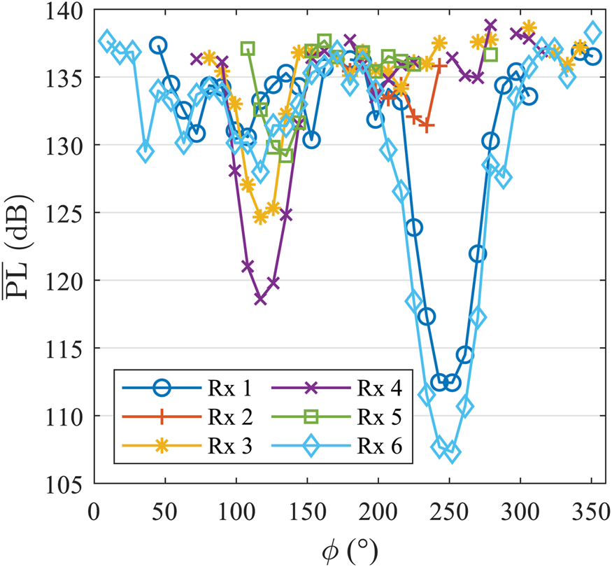
Fig. 13. $\overline {{\rm PL}}( \phi )$ at the six Rx locations.

Fig. 14. Spatial representation of $\overline {{\rm PL}}( \phi )$ .
.
For Rx 1 and 6, ϕ min matches the direction of the specular paths well. In case of Rx 3 and 4, there is a mismatch in the order of an angular step of 9° between ϕ min and the specular paths. The specular paths are within the HPBW of the Rx antenna at ϕ min for Rx 3 and 4. So the mismatch could be explained by multipath fading, which is discussed in section “Likelihood of multipath fading”. A different cause could be blockage by trees in or close to the specular paths. The mismatch is in the range of 20° − 25° for Rx 5. This could be due to the specular path of Rx 5 being at the estimated boundary of the red zone in Fig. 10. This predicted specular path is also close to the edge of the building where a tree is in the specular path. $\overline {{\rm PL}}_{ {min}}$ , the minimum PL, is highest at Rx 2, where no specular path is possible. $\overline {{\rm PL}}_{ {min}}$
 is 19 dB larger at Rx 2 compared to Rx 1, which is a nearby location with a specular path. The larger $\overline {{\rm PL}}_{ {min}}$
 at Rx 1 compared to Rx 6 could be explained by blockage from the obstructions discussed in section “Measurement scenario”.
5.2 Likelihood of multipath fading
A comparison of the PL at the different measured frequencies gives insight into the likelihood of multipath fading. Figure 15 depicts PL(f,ϕ min) and ΔPLmax, which is the maximum variation in PL over frequency at ϕ min. ΔPLmax is less than 1 dB for Rx 1 and 6, which suggests that there is no significant multipath fading in these measurements, where a strong specular component is present. ΔPLmax is 7 dB at Rx 2. The combined uncertainty with a confidence level of 95.45% is 1.1 dB at the maximum measurable PL, so the variation in PL at Rx 2 is not due to the uncertainty of the measurement setup and is caused by multipath fading. For Rx 3–5, ΔPLmax is between 3 and 6 dB and also affected by multipath fading. In [Reference Rappaport, Sun, Mayzus, Zhao, Azar, Wang, Wong, Schulz, Samimi and Gutierrez23], the effect of small-scale fading is investigated by moving an Rx over a 10 wavelengths long track at an interval of a half wavelength. A 6 dB fading variation of the main peak in the power delay profile (PDP) is reported there and indicated as having little influence on the AOA and received power level of multipath signals. Although no direct comparison can be made between power variation in a PDP and in the frequency domain, this shows that such variation in measured PL can also be expected in wideband channel measurements. Measuring more frequency points in a wider frequency band would improve the fading detection. In this work, the effect of multipath fading is reduced by averaging over frequency.

Fig. 15. PL for ϕ min at the measured frequencies. ΔPLmax is the maximum variation in PL between the measured frequencies at ϕ min.
5.3 Comparison of measured ${\overline {{\rm PL}}}_{ {min}}$ and FSPL

Figure 16 depicts $\overline {{\rm PL}}_{ {min}}$ and the FSPL for a distance equal to the path length of the corresponding specular path of Rx 1 and 3–6. The FSPL is averaged over frequency. The path via ϕ min is used in case of Rx 2, where no specular path is present. The excess loss at Rx 6 is <1 dB, which indicates that a building like B2 can be a very good specular reflector. The excess loss for Rx 1 is 9 dB. This larger excess loss compared to Rx 6 could be due to blockage by the obstructions in front of B2 and because the specular path does not intersect with the square flat surface of B2. Only 9 dB excess loss is measured at Rx 4 for a double specular reflection. It cannot be conclusively determined which parts of this loss are due to reflection loss, fading, and blockage by obstructions. The excess loss of 28 dB at Rx 2 suggests that the lack of a specular path significantly increases the PL. This observation is supported by the relatively large PL for ϕ pointing toward B2 at Rx 3–5 as can be seen in Fig. 14.

Fig. 16. Excess loss of $\overline {{\rm PL}}_{ {min}}$ with respect to the FSPL corresponding to the specular paths as depicted in Fig. 10.
6. Conclusion
A narrowband mm-wave measurement setup consisting of low-cost and ubiquitous hardware is presented in this paper. The measurement time and accuracy of this setup are improved by a measurement algorithm, which allows for measurements in a small frequency span despite the relative frequency drift between the Tx and Rx.
The uncertainty analysis of the measurement setup shows the impact of receiver noise, amplifier linearity, general system impairments, and antenna misalignment on the measurement accuracy. A theoretical model of the impact of receiver noise on the measured signal power is derived and verified with measurement data. This model is applied in Monte Carlo simulations to show how averaging of snapshots improves the measurement uncertainty. In the measurement campaign on specular building reflections, a 1 kHz RBW and 10 snapshots are used to enable PL measurements up to 139 dB. The combined uncertainty with a 95.45% confidence level is 1.1 dB at the maximum measurable PL and 0.3 dB in the case of low PL, where the uncertainty due to receiver noise is negligible.
The presented measurement campaign on specular building reflections shows that single- and double- specular building reflections are the main propagation mechanism in the measured NLOS area. The measurements show an excess loss of 1–9 dB for single-building reflections and 9–20 dB for double-building reflections with respect to FSPL. There is a good agreement between the specular path and the angle of minimum PL for single-building reflections. This agreement is less accurate in case of a double-building reflection, which is possibly caused by blockage from obstructions and/or multipath fading. An excess loss of 28 dB is measured for a single reflection without a specular path. These results support the hypothesis that buildings could be used as efficient mm-wave specular reflectors to increase the coverage in NLOS areas.
Acknowledgment
This work is part of the Flagship Telecom collaboration between KPN and the Eindhoven University of Technology.
 Robbert Schulpen received his M.Sc. degree (cum laude) in electrical engineering from the Eindhoven University of Technology in 2017. He is currently pursuing his Ph.D. degree in electrical engineering at the Eindhoven University of Technology. His research interests include millimeter-wave channel characterization and channel sounder design, calibration, and verification.
 Sander Bronckers received the M.Sc. degree (cum laude) in electrical engineering from Eindhoven University of Technology (TU/e), The Netherlands, in 2015. In 2018, he was a visiting researcher at NIST (Boulder, Colorado) on antenna measurements in reverberation chambers. He obtained the Ph.D. degree (cum laude) in electrical engineering in 2019, within the electromagnetics group at TU/e, on design and measurement techniques for next-generation integrated antennas. He is currently an assistant professor on Metrology for Antennas and Wireless Systems at TU/e. His research interests include antenna measurements in reverberation and anechoic chambers, channel sounding and emulation, and RF material characterization.
 Bart Smolders received his Ph.D. degree in electrical engineering from the Eindhoven University of Technology (TU/e) in 1994. He is an expert in smart antenna systems and worked at TNO, THALES ASTRON, and NXP semiconductors. Since 2010, he is a full-time professor at the TU/e in the Electromagnetics Group with special interest in smart antenna systems and applications. He currently leads several large research projects in the area of integrated antenna systems for 5 G/6 G wireless communications and radar. Next to his research activities, he is the dean of the Electrical Engineering department. More details can be found at: https://www.tue.nl/en/research/researchers/bart-smolders/
 Ulf Johannsen received his Dipl.-Ing. degree in communications engineering from Hamburg University of Technology (TUHH, Germany) in 2009. In 2013, he obtained his Ph.D. in electrical engineering from Eindhoven University of Technology (TU/e, the Netherlands). From 2013 until 2016 he worked as a Senior Systems Engineer at ATLAS ELEKTRONIK GmbH (Bremen, Germany), where his role was system designer and engineering manager on autonomous underwater vehicle (AUV) systems with sonar payloads. In 2016, he was appointed Assistant Professor with the Electromagnetics group at the TU/e department of Electrical Engineering. His research interest is focused on millimetre-wave antenna systems and antenna integration. Dr. Johannsen is chair person of the IEEE Benelux joint AP/MTT chapter, member of EuMA, and an associate member of INCOSE.


 Open access