


Introduction
The previous decade has witnessed significant advances made in the automotive sector. With the industry targeting complete or at least partial autonomous driving in the next 5 years, it becomes necessary to also take a few moments to consider the automated parking function of cars. This is a crucial function which is expected to be standard in almost all currently sold premium segment cars, and is gradually making inroads in the lower segment ones as well. Originally, parking functions were implemented based on the perception information delivered by ultrasound sensors [Reference Carullo and Parvis1, Reference Nascimento, Cugnasca, Vismari, Camargo Junior and de Almeida2]. Ultrasound sensors, however, are much more vulnerable to delivering erroneous data dependent on external factors, for example, a thin film of rain water on the surface of the sensor can induce false-positive detections. In addition, they are also susceptible to performance degradations in the presence of wind and sources of external noise.
On the other hand, radar sensors are much less susceptible to being influenced by external factors. Thus parking assistance systems are becoming increasingly dependent on radar sensors [Reference Waldschmidt and Meinel3]. Radars are inherently adept at resolving moving objects by discriminating them based on their Doppler response, since this is a function of velocity [Reference Winkler4].
However, for parking applications, where most objects are normally immobile, it is crucial to have the ability to resolve stationary targets. The most promising radar technique for achieving fine resolution images of parked cars and other immobile objects is synthetic aperture radar (SAR). There have been numerous implementations of automotive SAR which have been published in recent times [Reference Huaming and Zwick5–Reference Gisder, Meinecke and Biebl12]. Initially, it was necessary to adapt the SAR algorithms for automotive scenarios and also to examine the effects of motion on SAR [Reference Huaming and Zwick5, Reference Iqbal, Sajjad, Mueller and Waldschmidt7]. The influence of false positions of the radar were also examined. Building on these fundamentals, it was thus possible to build a SAR demonstrator and have it image a typical parking scenario [Reference Wu, Zwirello, Li, Reichardt and Zwick6]. The motion compensation was accomplished with the combination of a gyroscope and an accelerometer.
In a further advancement toward making SAR a viable solution for facilitating the search for parking spaces, a graphical processing unit (GPU) was employed for processing. The time-domain backprojection algorithm was implemented on a GPU such that the backprojection algorithm [Reference Yegulalp13] could be processed in parallel. This considerably reduced the time needed to generate an image of the target scenery to a few seconds [Reference Gisder, Harrer and Biebl9, Reference Harrer, Pfeiffer, Löffler, Gisder and Biebl10, Reference Gisder, Meinecke and Biebl12]. This represented a significant step from “offline” processing to “online” processing. In offline processing, data are first collected and then processed later on a PC which may not even be located in the vehicle used, while in online processing, the data are processed immediately as soon as it is ready and new data are simultaneously acquired in the background.
A necessary requirement for automotive SAR is a relatively high radar duty-cycle. This implies that the cycle time (the amount of time before the data from a new block of chirp sequences is available) should be as short as possible. Usually this is a limitation due to the hardware and is also dependent on the modes of operation of the radar. It is not perceivable that a radar will be dedicated solely for SAR imaging, hence there may be gaps in time where no chirps are available. It has been shown that this gap may be bridged by zeros or in the best case, the missing chirps may be reconstructed via compressed sensing [Reference Iqbal, Schartel, Roos, Urban and Waldschmidt11].
The results presented in this paper are the outcome of continued efforts to improve upon the status previously published by the authors [Reference Iqbal, Löffler, Mejdoub and Gruson14]. In this article, a deeper discussion will be presented of the radar signal processing, ego trajectory calculation as well as time synchronization. Improvements in processing and algorithms made over the previous paper will be highlighted in each respective section.
Measurement set-up and parameters
The car used for all SAR measurements is displayed in Fig. 1. The radar sensors mounted to the car are encircled in red. The front sensor is used to calculate the ego trajectory of the vehicle, while the sensor placed at the rear-right corner of the car is used to acquire measurements for SAR processing. The duty cycle of the rear-right sensor is 97% when considering the time for used chirps over the complete cycle time. The time during which the transmitter is switched on is defined as the quotient of on-time to chirp-time (as illustrated in Fig. 2). Thus the in-chirp duty cycle is 44% which results in a total duty cycle of 43%.

Fig. 1. Measurement set-up for SAR. Height of rear-right sensor: 40 cm, height of front sensor: 50 cm.

Fig. 2. Visual explanation of in-chirp duty cycle. f 0 denotes the start frequency.
The radar sensors mounted to the car are based on a development platform back-end with a front-end (antennae) analogous to that of the sixth-generation short-range radar (SRR) [15]. Since these are pre-series research specimens, the size of the sensor does not reflect the eventual size of the radar that will be commercially available.
The parameters for both radar sensors are summarized in Table 1. The bandwidth for the front sensor was initially only 166 MHz, but with an update in the configuration, the bandwidth was increased to 1 GHz. This shall be discussed in greater detail in section “Radar processing chain”.
Table 1. Parameters for the front radar (ego trajectory calculation)

The time-domain backprojection algorithm [Reference Yegulalp13] was employed for the processing of the raw radar measurements into SAR images. The SAR processing was implemented on a GPU to exploit the faster processing speed and higher available memory. The resolution of the calculated SAR images has been set to 5 cm in both the azimuth and range directions. This was done to make a trade-off between the quality of the processed SAR images and the processing time. A finer resolution would increase the computational efforts and slow down the processing chain. The actual resolution in range is 15 cm given by the bandwidth of the transmitted signal. It has been artificially enhanced to 5 cm with the help of zero padding.
The details of the processing chain are discussed in section “Rear-right radar with SAR processing”.
Ego trajectory calculation
For the correct processing of SAR images, an accurate trajectory is of utmost importance. Due to previous experience with GPS and vehicle dynamics based dead reckoning, it was decided to deploy a radar-based solution for the trajectory calculation. The other mentioned approaches could not deliver trajectory information with the accuracy required to generate SAR images.
The radar-based approach for trajectory estimation has already been reported in literature [Reference Checchin, Gérossier, Blanc, Chapuis, Trassoudaine, Howard, Iagnemma and Kelly16–Reference Kellner, Barjenbruch, Klappstein, Dickmann and Dietmayer18]. One important difference to the work published by Kellner et al. ([Reference Kellner, Barjenbruch, Klappstein, Dickmann and Dietmayer18]) is the possibility for the calculation of the yaw rate of the car. For more accurate yaw rate calculations however, at least one more radar is required with a tilted mounting position. A crucial condition for this approach is that the number of stationary targets in a scenario must top the number of dynamic targets. In order to make the complete system more reliable in situations where the number of dynamic detections exceeds the number of static detections, the vehicle dynamics (wheel speeds available over vehicle bus) could be used to bridge the gap. Indeed, the information available from the vehicle dynamics could also be fused with the ego velocity calculated as described below, with the use of a Kalman filter. As the quality of vehicle dynamics is inherently low, a fusion-based approach would mitigate the poor quality and reduce the rate of failure significantly.
The radar acquiring measurements for trajectory calculation was affixed to the front of the measurement vehicle so that it is always aligned with the heading vector of the car. This way the measurements delivered by the sensor can be evaluated to calculate the driven distance in the direction of the heading vector (in positive x direction). To calculate the trajectory involving lateral movements, a second sensor mounted at an angle is necessary. However, for the scope of the research presented here, only straight driven trajectories are considered. SAR with curved trajectories will be considered at a later stage.
The functional concept is clarified in Fig. 3. The radar is placed at the front of the car while the targets are represented by the orange dots in front of the car. The velocities of the targets (v t) are denoted in orange while the radial velocities (v r) of the targets are visible in black. The angle denoted by θ is the angle between the particular target's radial velocity and the radar bore-sight. This is the azimuth angle as seen by the radar. The small coordinate system to the right of the car illustrates the orientation and direction of the x, y, and ω axes. Below the car is a set of axes representing the velocity against the azimuth angle (ω). Here the various stationary targets are plotted at their respective azimuth angles corresponding to the component of their velocity which results in the radial velocity. At ω = 0, the velocity vector aligns perfectly with the heading vector and thus gives the velocity of the car. Dynamic targets are not shown on the parabola since they are out-liers and do not fall on the curve.
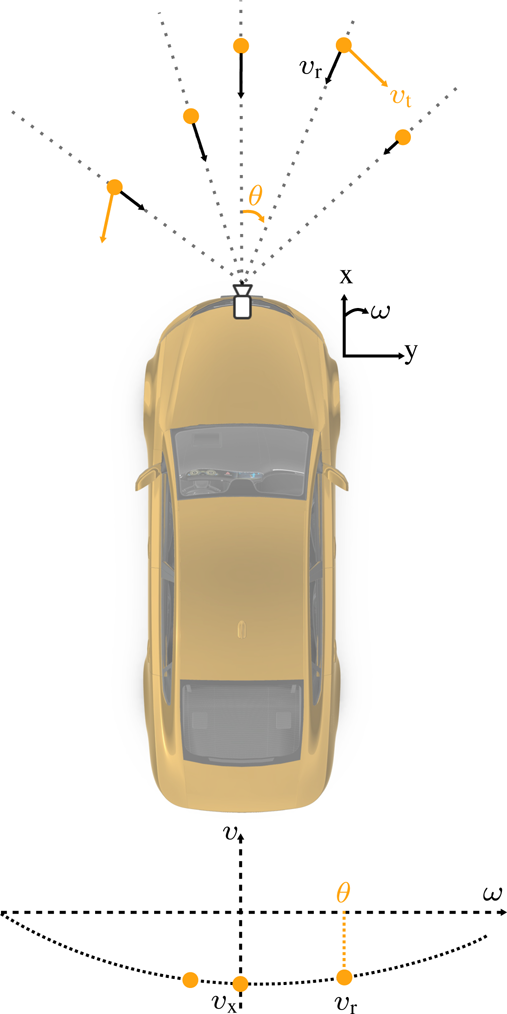
Fig. 3. Diagram clarifying the position of the radar and targets [Reference Kellner, Barjenbruch, Klappstein, Dickmann and Dietmayer18]. Target velocity (v t) vectors are displayed in orange while the radial velocity (v r) vectors in black. The coordinate system to the right of the car shows the orientation and direction of x, y, and ω axes. In the bottom part of the figure, the velocities are plotted against the azimuth angle (ω) for the stationary targets. v x represents the ego velocity since it is in the same direction as the heading vector.
A generalized radar mounting position is shown in Fig. 4 along with the heading vector (direction of travel of the car), and the two angles between the heading vector and radar bore-sight (θ) and between the target and radar bore-sight (ρ). This will help to gain a clearer picture of the processing steps and the equations which will be introduced in the following paragraphs.
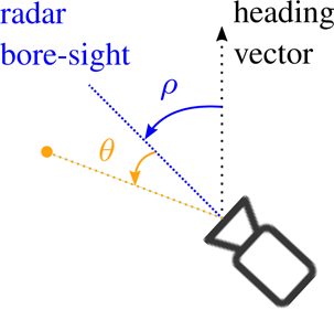
Fig. 4. Generalized radar mounting position along with a visual definition of the heading vector, the angle between the heading vector and the radar bore-sight (ρ) and the angle between the radar bore-sight and the target (θ).
The processing steps for the ego trajectory calculation are shown with the help of a flow diagram in Fig. 5. The process starts with the arrival of new detections from the front radar. Once new data are available, the Random Sample Consensus (RANSAC [Reference Fischler and Bolles19]) process is started which encompasses numerous processing stages as displayed in Fig. 5. The processing is programmed such that, a single thread is dedicated for the processing stages in one iteration. Thus, depending on the capability of the computer, as many processes are started as the maximum number of threads which can be simultaneously executed.

Fig. 5. Flow diagram depicting the processing steps for the ego trajectory calculation.
Each process selects detections from the new data at random and builds a velocity model based on these detections. Each detection includes the azimuth angle (ρ) and the radial velocity (v r) of the target it represents. The velocity model calculates a hypothetical fit for each data point according to the relationships defined by the following equations,

where v x, v y are the components in Cartesian coordinates of the instantaneous ego velocity and ω is the yaw rate. These terms constitute the output values of the ego trajectory calculation block. vr denotes the vector of radial velocities

comprising the velocities of each detection respectively. C+ is defined as the pseudo-inverse of the covariance matrix defined as

with U i = cos(θ i + ρ), V i = sin(θ i + ρ), W i = cos(θ i + ρ) · l s,x and X i = sin(θ i + ρ) · l s,y. The parameters l s,x and l s,y represent the sensor positions in the x and y dimensions, respectively.
Once the ego velocities and the yaw rate (v x, v y, and ω) have been calculated, an error function is used to discriminate the out-liers from the in-liers. The error function compares the calculated velocities with the radial velocities of the remaining detections by converting the radial velocities into their Cartesian components. If the difference (error) between the calculated and the actual velocities of the detections is larger than a set threshold, the detections are classified as out-liers. Next, the results are saved to memory and the stopping criterion is checked. If the stopping condition is satisfied, the best model over all the processes is found and returned. Based on this model, and the previous results, the traveled trajectory is calculated in both x and y dimensions. This result is then transferred to a ring buffer in memory from where the result can be recalled by the next block in the processing chain.
Radar processing chain
In the measurement set-up illustrated in Fig. 1 and discussed in detail in section “Measurement set-up and parameters”, there are two radar sensors being simultaneously used. For SAR processing, it is necessary to designate an ego position, x and y coordinates, to each and every chirp that is processed into the SAR image. In order to accomplish this, the front and rear-right radar sensors need to be time synchronized accurately. In the following sub-sections, the details of the time synchronization as well as the signal processing chains of both radars are discussed.
Precision time protocol (PTP)-based time synchronization
The precision time Protocol (PTP)-based timing architecture is depicted in Fig. 6. Here one of the measurement computers in the car is designated as a PTP-master and it is connected to a GPS receiver which is enabled to receive time messages with an accuracy down to tens of nanoseconds (< 100 ns). The accuracy of the timestamps, however, is dependent on the clock frequency of the individual slave devices which receive the timestamped data. The radar sensors have been verified to provide timestamps with an accuracy of at least 200 ns.

Fig. 6. PTP network architecture for accurate time synchronization between the front (calculate trajectory) and rear-right (SAR measurements) radar sensor.
Once the PTP-master has a solid GPS fix, the time is shared with a PTP-capable switch which itself acts as a master for the two radar sensors and also any other instruments or devices which subscribe to PTP messages on the network. All PTP messages are distributed over a 1 Gbps Ethernet connection.
Using this approach, it is guaranteed that the chirp sequence is stamped with the time at the source. This way any delays and latencies due to network impairments are ruled out.
Front radar
The processing steps involved in the calculation of the ego trajectory are illustrated in Fig. 7. As was mentioned in section “Measurement set-up and parameters”, the sensors used are development back-ends delivering digitized IF signals in time domain. Therefore, in the first step, fast Fourier transforms are carried out in three dimensions producing what is referred to in the automotive industry as a radar cube (comprising range, Doppler, and azimuth angle of targets).

Fig. 7. Processing chain and data flow diagram showing detailed steps for the front sensor.
In the next step, a constant false alarm rate threshold [Reference Rohling20] based technique is used to identify and locate peaks from the radar cube. Essentially, notable reflections are separated from clutter and noise. The so-called peaks are then potential targets which are processed in the next step into valid detections. In order to validate peaks into detections, various algorithms are used to discriminate actual targets from ghost targets or other Doppler artifacts which, dependent on the scenario, may be present in the signal.
All the processes depicted in Fig. 7 are executed on a GPU and the interprocess exchange of data is done via shared memory.
Compared to the previous software status of the front sensor, a couple of important updates have been made thereby leading to improvements in the overall chain:
(1) Field of view: In the software version used previously in [Reference Iqbal, Löffler, Mejdoub and Gruson14], though the radar had a broad field of view, only those detections could be processed which were located in a + / − 30° cone from the radar bore-sight. This was due to the nature of how software development is carried out in versions and its effects can be visually seen in Fig. 8. Here the radar detections are plotted in Cartesian coordinates. The red lines depict the + / − 30° region centered around the radar bore-sight. This is a very narrow region and the radar detections available from here might be too little for an accurate trajectory calculation dependent on the characteristics of the location.
For example, it was noticed that the accuracy of the calculated ego trajectory was significantly lower when the car was driven toward a wide wall or other structure which extends far to the right and left side of the car. Upon investigation, it was discovered that such extended targets like walls behave as mirrors for the transmitted waves and thus targets behind the car appear to the radar to actually be in front. However, the Doppler and azimuth angle information is distorted due to reflection from the wall, leading to errors in the trajectory calculation.
By updating the software and thereby increasing the field of view to + / − 80°, a higher number of detections are thus available and the mirroring effects from wall-like structures can be more easily filtered out by RANSAC. Radar detections of a similar scenario, as in Fig. 8, obtained from the updated software chain are depicted in Fig. 9. It is immediately apparent that the number of detections has increased enormously.
(2) Increased bandwidth: In another update, a high-resolution configuration for the radar was created which supports a higher bandwidth of 1 GHz. To accommodate the high-resolution mode, the maximum range of the sensor was reduced to approximately 40 m as the chirp length remained constant.
The result of the high-resolution mode is a much improved quality of radar detections even when the car approaches large extended structures like walls. In relatively closed locations, the high-resolution mode is the appropriate mode for trajectory estimation, while in open spaces the older configuration with a coarse resolution will suffice.
The error percentage of the calculated trajectories using the pre-update and updated software versions are summarized in Table 2. The measurements were carried out in the same closed location (approaching a wall) and repeated multiple times for both software versions. The values shown in Table 2 are chosen from one representative measurement of each version.
Table 2. Accuracy comparison of the calculated trajectories

The error as expected is large when the trajectory is calculated with the older software version. This error in the trajectory translates into blurry and unfocused SAR images, as each SAR chirp is assigned an erroneous location on the traveled trajectory. Using the updated software version, this error has been reduced to a level which is in the tolerance range.

Fig. 8. Plot of detections obtained from output of the older processing chain.
Rear-right radar with SAR processing
The architecture and processing blocks for the data from the rear-right sensor are depicted in Fig. 10. The data from the front sensor are first processed into trajectory information and then the trajectory points are pushed into a ring buffer as already discussed in detail in section “Radar processing chain”.
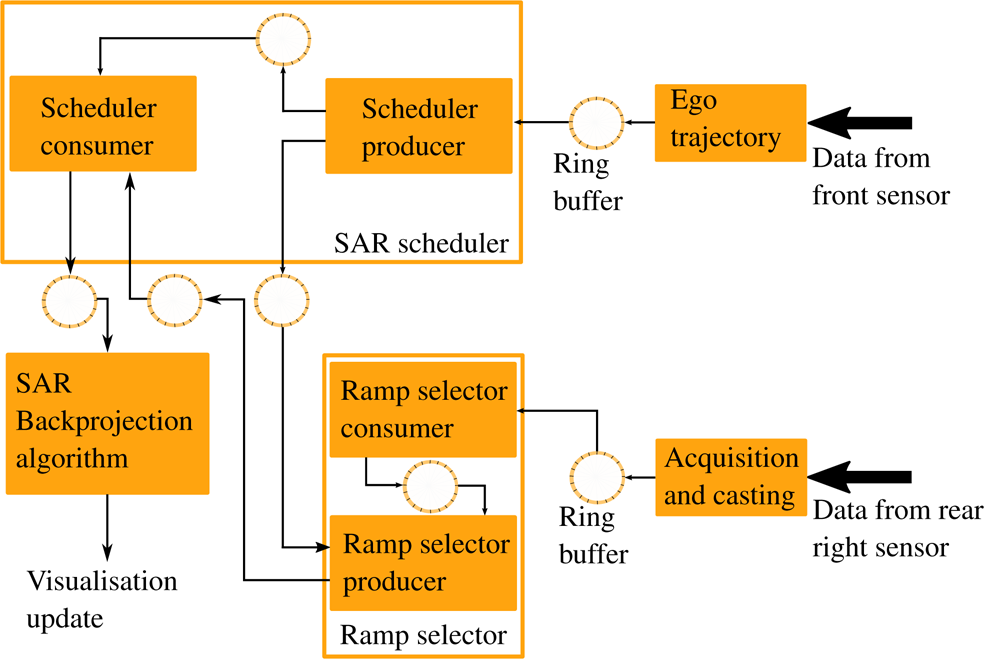
Fig. 10. Data flow diagram depicting how and where data from both the front and rear-right radar sensors are processed.
The trajectory points are fetched from the ring buffer by the SAR scheduler producer thread where they are filtered into waypoints such that each waypoint is equidistant at an interval of 1 mm. This grid of trajectory waypoints is shared via ring buffers with the scheduler consumer as well as the ramp selector producer threads.

Fig. 9. Plot of detections obtained from output of the updated processing chain.
Meanwhile the data from the rear-right sensor consisting of FMCW ramps meant to be processed into SAR images are fetched from the ring buffer by the ramp selector consumer thread. The consumer thread of the ramp selector is tasked with creating a timestamped grid of radar ramps. The block of ramps is already stamped with the UTC time directly in the sensor, as mentioned in section “Precision time protocol (PTP)-based time synchronization”). Using these timestamps, every individual ramp is assigned a unique UTC timestamp via interpolation from the block timestamp issued by the sensor. The timestamps grid corresponding to the radar ramps are pushed into the ring buffer once ready.
In the next step, the producer thread of the ramp selector fetches the next trajectory waypoint prepared by the scheduler producer as well as the ramps grid from their respective ring buffers which are illustrated in Fig. 10. The ramp selector producer then searches for a ramp which matches the trajectory waypoint timestamp. The trajectory waypoints are treated as masters, since one FMCW ramp is needed every 1 mm, since to avoid aliasing a measurement is needed every λ/4. The wavelength at 77 GHz is approximately 4 mm, thereby one ramp every millimeter. Though depending on the ego velocity, there may be multiple ramps available for a particular trajectory point. Therefore, a corresponding ramp is allotted to each trajectory waypoint and not the other way around.
Once the closest ramps (in time) to a queried trajectory waypoint are found, the complete block of the ramps is transferred to a ring buffer, from where the scheduler consumer can fetch them. The scheduler consumer interpolates the radar ramps to the requested trajectory waypoint timestamp. Once this has been accomplished, each 1 mm waypoint is associated to its corresponding interpolated radar ramp.
These matched pairs of radar ramps and trajectory waypoints are then pushed into the next ring buffer from where the SAR backprojection algorithm can access them. The backprojection algorithm has been programmed such that an update to the SAR image is calculated every time new trajectory and SAR ramps are available from the previous 12 cm worth of trajectory. This is to ensure that updates are quick enough without completely blocking the process on the one hand, while on the other hand the updates are substantial enough to provide new information. An update every centimeter, for example, would block the process and each update to the SAR image would have less significant information content, since not a lot of new information can be gathered by traveling just 1 cm further.
The SAR image calculation through the backprojection algorithm has been implemented on a GPU, which requires <76 μs to process a ramp corresponding to a trajectory of 1 mm in length. Compared to the early stages of development where the backprojection was implemented in MATLAB, the processing on the GPU is approximately 45 times faster. Therefore, the calculation time has been reduced to such an extent that the SAR image is ready in real-time, that is within a couple of seconds after measurement.
After each update has been processed, a new SAR image is sent to the visualization block which updates the image on the screen. Currently, for demo purposes, the SAR image is displayed as a picture on a screen; however, the calculated SAR values can from this instance be used as an input for further radar processing algorithms.
In an update to the SAR processing reported in [Reference Iqbal, Löffler, Mejdoub and Gruson14], the ramp selector described above was modified to tackle the issue of missing chirps illustrated in Fig. 11. Due to the duty cycle as well as hardware restrictions, there are some gaps between blocks of chirps where no ramps are available. At low ego speeds, the missing ramps are hardly noticeable since enough adjacent ramps are available to enable successful interpolation. However, at higher speeds, attempting to recreate the missing ramps through interpolation will lead to phase errors, since the adjacent ramps are spatially too far apart. This leads to blurred SAR images.

Fig. 11. Diagram illustrating how some chirps are missing between two blocks of chirp sequences.
To resolve this issue, the ramp selector simply substitutes zeros in place of the missing chirps instead of attempting to recreate them via interpolation. This way blurring in SAR images even at high speeds is significantly reduced as shown in section “Measurement results”.
Measurement results
One of the first measurement scenarios is displayed in Fig. 12. Along with the car, a small scooter, child's car, and bike are the objects of interest which need to be seen in the image as important targets which a parking car needs to avoid driving over.

Fig. 12. The first measurement scenario. Red arrow indicates the driving direction and the green arrow shows the direction of the SAR sensor bore-sight.
The processed SAR image for the scenario from Fig. 12 is shown in Fig. 13. The contour of the car can clearly be made out while the scooter and bicycle in particular seem to be merged into the car. This occurs since the distance from the bicycle and scooter to the car is small (<1 m). The scooter is encircled in purple around 5 m in azimuth while the bicycle has a green ellipse around it at approximately 11 m in azimuth. The child's car, highlighted in white, though is very easy to make out since it is further away from the car.

Fig. 13. Processed SAR image of scenario from Fig. 12. Trajectory start point is in the top left corner. Ego speed is 10 km/h.
This scenario was chosen to represent a challenging parking situation where a large target (car) has smaller targets in the direct vicinity. The smaller targets have lower radar cross-sections especially when one keeps the orientations of the scooter and bicycle in mind, from Fig. 12. The scooter is lying such that its body is slanted and most of the incident radar energy is reflected away, while the bicycle is placed such that its slim front is oriented toward the radar. Both these targets, therefore, can easily be overlooked if classical radar imaging is used. Using SAR, even though it may not be possible to clearly discern the contour of the scooter and bicycle when placed so close to the car, it is nevertheless possible to see that the respective space is occupied by a target.
In order to generate a control image of the objects from Fig. 12, the measurement was repeated but this time the spacing was increased as shown in Fig. 14. The scooter is deep in the background (encircled in red), lying with its broad metal bottom oriented toward the radar. The bicycle has also been rotated, so that the larger side is seen by the radar. This measurement allows imaging of the objects without being influenced by the car's signature. The SAR image from this scenario can be seen in Fig. 15.

Fig. 14. Repeat of scenario from Fig. 12 with greater spacing between the objects. Red arrow indicates the driving direction and the green arrow shows the direction of the SAR sensor bore-sight. The scooter is encircled in red in the background.

Fig. 15. Processed SAR image of scenario from Fig. 14. Trajectory start point is in the top left corner. Ego speed is 20 km/h.
The effect of the orientation of the scooter and bicycle is immediately obvious when Fig. 15 is compared with Fig. 13 corresponding to the previous scenario. In Fig. 15, the scooter's distinct shape is readily visible including the long metal rod used for steering. The bicycle and small child's car can also be easily recognized.
These two scenarios represent an important criterion for parking applications. That is the detection and avoidance of small targets which may be lower in height than the car and may not always be visible to the driver. Nonetheless, with help from SAR, it is possible to detect such targets and avoid them.
In order to gauge the imaging capability at higher speeds, the black car from Fig. 14 was parked next to a concrete block and this scenario was recorded at an ego speed of 45 km/h. The SAR image thus obtained is displayed in Fig. 16. The image is as sharply focused as the measurements obtained at slower speeds, with no observable streaking. As mentioned in section “Rear-right radar with SAR processing”, by inserting zeroes in place of the missing chirps instead of interpolating, the phase errors can be minimized. This has a direct result on the quality of the SAR image. The contour of the car is visible directly after 5 m in azimuth until 10 m and a range of 4 m. The block of concrete can also be seen just before 15 m in azimuth and a range of slightly more than 6 m.

Fig. 16. SAR image of car parked next to a block of concrete. Trajectory start point is in the top left corner. Ego speed is 45 km/h.
Finally, a scenario was chosen to demonstrate the capability of the processing chain to handle long trajectories. The scenario chosen for this is shown in Fig. 17. The two sub-figures show different parts of the same scenario for easy cross-reference between the SAR image and the optical photo-based ground truth. The objects shown in Fig. 17(a) correspond to the initial part of the trajectory while the scenario depicted in Fig. 17(b) illustrates the various objects in the latter part of the measurement.

Fig. 17. Measurement scenario with various target objects and a trajectory of 100 m. The two pictures show different portions of the same measurement trajectory. (a) Initial part of the measurement involving a parked car, curved kerb, and some trees. (b) Latter part of the measurement consisting of a perpendicular fence, a sign board, and a building.
The processed SAR image for the long trajectory scenario from Fig. 17 is illustrated in Fig. 18. The most striking feature of the SAR image is the kerbstone which runs along almost the complete trajectory. In two places, the kerbstone curves away from the ego vehicle which can also be easily seen in the SAR image. The first line from the top is the actual kerb while the second line which runs parallel to the first one corresponds to the boundary where the kerbstone comes to an end and the grass begins. The car parked between the first curved kerbstone can be easily seen at approximately 12 m in azimuth.

Fig. 18. Processed SAR image of scenario from Fig. 17. Trajectory start point is in the top left corner. Ego speed is 25 km/h.
The large trees visible in Fig. 17 can also be made out in the SAR image between 18 and 67 m in azimuth. The reflections from the trees are not strong since the numerous leaves and branches present a diffused target which either reflect the incident waves away from the radar or depolarize the incoming waves such that the radar cannot receive them. Additionally, the foliage penetration depth is very low at 77 GHz, therefore there are very few reflections from tree trunks.
After the trees, just before the kerb curves into the street, there is a fence which is outlined by a blue ellipse in Fig. 18. It is possible even to see the individual metal posts holding the fence together in the SAR image. Right after the fence is the metal sign board with various company names on it. This sign board is encircled in green in Fig. 18.
Upon close scrutiny of Fig. 17(b), it is possible to see a small dark porch just in front of the door to the large building. This porch can also be seen in the SAR image highlighted in white. Right after this the kerbstone continues further alongside the wall of the building. For this scenario, a trajectory of 100 m was driven along, while measurements were recorded. This measurement result is a testament to the accuracy of the calculated trajectory, since even small errors in trajectory can accumulate and cause major deterioration in the SAR image, particularly toward the end of the trajectory. In this case however, the SAR image has the same sharp focus toward the end as at the start.
Conclusion
In this paper, a high-resolution radar imaging implementation is presented which is capable of delivering high-resolution SAR images of stationary targets in real time. Coupled with the fact that the hardware used for this implementation can easily be replaced by embedded systems and thus can be developed into a series product, making automotive SAR a competitive enabler for automated parking functions.
Additionally, SAR can also be used to create high-resolution maps which can be shared (e.g. through a cloud) between highly autonomous vehicles, thereby making automated driving in urban environments easier. This way a vehicle which itself may not be SAR-capable can benefit from the maps created by other vehicles which created and updated the map a few minutes or even seconds ago.
It has been shown here with the help of measurements that the signal processing chain is quick enough to output high-resolution images with high accuracy even at large ranges and speeds in excess of 45 km/h. The previous issue of streaking at high speeds reported in [Reference Iqbal, Löffler, Mejdoub and Gruson14] has also been resolved.
Hence, it can safely be said that the combination of a SRR and SAR can outperform ultrasonic parking sensors in range, accuracy, and sensitivity. Plus SAR does not suffer deterioration in performance from wind, rain, snow, and external noise, such as from construction equipment, like ultrasonic sensors do.
 Hasan Iqbal obtained his B.Sc. and M.Sc. degrees in Electrical Engineering from COMSATS University in Islamabad, Pakistan and Ulm University in Ulm, Germany in 2008 and 2013, respectively. He is currently working as an Algorithm Developer for the next generation of novel and innovative radar sensors and systems at Continental, Business Unit Advanced Driver Assistance Systems (ADAS).
 Andreas Löffler received his Diploma degree in Electrical Engineering from the Friedrich-Alexander University of Erlangen-Nuremberg, Germany in 2006. He is currently working at Continental, Business Unit Advanced Driver Assistance Systems (ADAS) as an Expert in Advanced Radar Sensors and Systems with focus on the next generation of radar sensors.
 Mohamed Nour Mejdoub graduated with M.S in Computer Science from Ecole Nationale des Sciences de l'Informatique Tunis in 2012. He also received degrees in Autonomous Driving Cars and Robotic Software in 2017 and 2019, respectively, from Udacity. His current research interests include tracking, sensor fusion, and machine learning.
 Daniel Zimmermann received the B.Sc. and M.Sc. degree in Electrical Engineering from RWTH Aachen, Germany, in 2016 and 2020, respectively. He is currently working at Continental, Business Unit Advanced Driver Assistance Systems (ADAS) in Radar System Engineering as HiL System Architect.
 Frank Gruson is Head of Advanced Engineering Radar at ADC Automotive Distance Control Systems GmbH (a Continental Company) in Lindau, Germany. Since 2007 he has served Continental in numerous positions in the area of RF development and systems engineering. Frank is strongly engaged in the worldwide harmonization of frequency spectrum for automotive radar sensors, both on European level (ETSI) and on international level. Frank contributed to several successfully funded research projects on EU and BMBF level, such as KOKON, RoCC, MOSARIM, SafeMove, IMIKO and VIVALDI. Prior to joining Continental, Frank was active in semiconductor technology, RF chipset design, application engineering and marketing in the semiconductor business and in the Research Center of the Daimler AG in Ulm. Frank received his Masters degree in Physics from the University of Ulm in 1994 and his PhD in Electrical Engineering in 2010.


 Open access