


Introduction
Due to the high number of mobile and satellite communication services, the electro-magnetic spectrum is getting more crowded and the resource “bandwidth” is becoming scarce. The performance of the filters especially at the output stage after amplification is very important to fulfill the stringent out-of-band rejection requirements of a transmitter system. Depending on the application of the filter to be designed, requirements in terms of near-band rejection, losses, and volume/weight are often in the focus of interest.
Transmission zeros (TZs) are important in the filter design process as the near-band selectivity of the filter can drastically be improved without increasing the filter order n and hence the associated losses [Reference Cameron, Kudsia and Mansour1]. Real- and complex TZs might be realized by destructive and constructive interference, respectively. The importance of complex pairs of TZs is mainly defined by the phase linearity constraints.
Nevertheless, the classical approach as comprehensive presented in e.g. [Reference Cameron, Kudsia and Mansour1] has fundamental limitations. TZs might only be realized by cross-couplings or extracted pole sections. The first type may lead to difficult to realize diagonal cross-couplings, which is often a severe problem especially in waveguide filters. Extracted pole filters are an interesting alternative but suffer from an increased footprint due to the need of non-resonating nodes which couple the extracted pole resonators [Reference Montejo-Garai and Rebollar2]. A further limitation is the theoretical maximal number of TZs n fz which is limited by the filter order n itself and cannot exceed it.
These limitations are circumvented in the set-ups presented in this paper. Different techniques for the generation of TZs are combined within one filter set-up, leading to in total up to eight real frequency axis TZs by a filter order of n = 4. Apart from classical destructive interference, bypass-couplings as proposed in e.g. [Reference Bastioli3, Reference Amari and Rosenberg4] are used to increase the total number of TZs. Additionally, a frequency-dependent coupling aperture [Reference Szydlowski, Lamecki and Mrozowski5–Reference Rosenberg, Amari and Seyfert8] is able to introduce one additional TZ by replacing a classical (non-resonant) coupling aperture. Furthermore, the direct source to load (SL) coupling is able to realize two types of TZs simultaneously. On the one hand, TZs are generated by the classical destructive interference while on the other hand dispersive/resonant TZs might additionally occur [Reference Miek, Reinhardt, Daschner and Höft9–Reference Mokhtaari, Bornemann, Rambabu and Amari12].
Four slightly different filter set-ups are presented in this paper which make use of some of the TZ generating mechanism or even all. This paper is organized as follows. Based on [Reference Miek, Morán-López, Ruiz-Cruz and Höft13], the basic filter set-up is shortly repeated in section “Basic filter set-up”. In section “Phase equalized filter with six TZs”, it is shown that the proposed set-up is able to realize a complex pair of TZs for phase equalization as well, leading to in total six TZs. The total number of TZs might be increased by using a double-slotted source to load cross-coupling aperture as described in section “Filter set-up with double source to load coupling” while section “Filter set-up with additional frequency-dependent coupling structures” exploits the use of frequency-dependent coupling apertures. Section “Conclusion” concludes this paper.
Basic filter set-up
The basic filter set-up was first proposed in [Reference Miek, Morán-López, Ruiz-Cruz and Höft13] and is repeated in Fig. 1 for the sake of clarity. The desired filter specifications are set to the lower and upper passband edge of f 1 = 14 GHz and f 2 = 14.25 GHz, respectively, while the desired return-loss in the passband is set to RL = 20 dB. Two TZs in the initial design are foreseen at normalized frequency f TZ,Lp = ±j2. The associated coupling topology is a quadruplet with a negative coupling factor between cavity one and four (m 14) [Reference Cameron14]. The synthesis of the initial filter dimensions is accomplished based on [Reference Cameron, Kudsia and Mansour1, Reference Hong and Lancaster15]. First, substructures (two cavities coupled by a blend aperture) are simulated to find the correct coupling factors in terms of eigenmode simulations. The length of the different cavities can be estimated by the loading as described in [Reference Cameron, Kudsia and Mansour1] Ch. 14.5. Finally, the fine tuning of the filter takes place by coupling matrix extraction and adjustment techniques using the Cauchy method [Reference Lampérez, Sarkar and Palma16]. Note that the filter dimensions obtained here are used as a basis for the further adaptions made in the next sections.

Fig. 1. Basic filter set-up for the realization of up to seven real frequency axis TZs. Dimensions are identical as proposed in [Reference Miek, Morán-López, Ruiz-Cruz and Höft13]. The dimensions of the waveguide are chosen according to the Ku-band standard: a = 15.7988 mm and b = 7.8994 mm.
For the realization of the two real frequency axis TZs, a negative cross-coupling between resonator one and four is required [Reference Miek, Morán-López, Ruiz-Cruz and Höft13]. Many approaches are known in the literature for the realization of negative coupling factors in waveguide filter techniques. Stacked filter topologies are a common solution as electric and magnetic couplings might easily be realized through the bottom/cover of a cavity. Depending on the position of the coupling aperture (e.g. near the side wall or in the center), the magnetic or even electric field coupling dominates [Reference Miek, Reinhardt, Daschner and Höft9, Reference Miek, Morán-López, Ruiz-Cruz and Höft10]. For lower frequencies, even small probes for the coupling of electric fields are possible [Reference Miek and Höft17]. Nevertheless, in higher frequency ranges, aperture couplings are preferred, as the tuning of e.g. probes becomes complicated and the losses increase. The solution used here for the realization of a negative coupling factor m 14 is to turn around the direction of the magnetic fields in oversized cavities as e.g. proposed in [Reference Rosenberg18]. Therefore, cavity two and four are designed to resonate at their basic TE 101 mode whereas cavity one and three resonate at the TE 102 mode. Figure 1(b) gives an overview over the relative positions of the cavities as well as the magnetic fields at center frequency. Note that the magnetic fields in adjacent cavities along the main-line are oppositely oriented to each other. The coupling factor of two adjacent cavities i and j is proportional to the electric and magnetic fields, which couple through the aperture according to (1).

By comparing the direction of the magnetic fields with the definition in (1), all main-line couplings realize a positive coupling factor. However, considering the cross-coupling aperture, it becomes obvious that a negative coupling factor between cavity one and four arises. The electric field component in (1) can be neglected in this case as there are only magnetic coupling apertures. Therefore, two TZs are generated by the destructive interference between cavity one and four.

However, as discussed in [Reference Miek, Morán-López, Ruiz-Cruz and Höft13], additional coupling paths between the source port and cavity two (m S2), the source port and cavity four (m S4) as well as cavity two and four (m 24) arise. The reason is that the basic TE 10 mode is excited in the oversized cavities one and three, realizing bypass couplings for the generation of an additional TZ above the passband of the filter. The corresponding field lines of the basic non-resonant modes are shown in Fig. 1(b) while the associated coupling scheme is shown in Fig. 2(a). A modeling of the bypass couplings with non-resonant nodes in the coupling scheme would be possible as well, but as discussed in [Reference Bastioli3] the design by using “classical” coupling paths is sufficient in the considered case.

Fig. 2. Coupling schemes of the filter set-up from Fig. 1: (a) set-up without direct source to load cross-coupling and (b) set-up with direct source to load cross-coupling [Reference Miek, Morán-López, Ruiz-Cruz and Höft13].
The filter of Fig. 1(a) was manufactured as a proof of concept in brass as a conventional H-plane filter. Tuning screws can be inserted in the cover of the filter at positions indicated by circles in Fig. 1(b). The measurement results in comparison to the simulation are shown in Fig. 3. Three TZs as expected by the simulation and the coupling diagram of Fig. 2(a) arise while a quality factor of Q u ≈ 2100 can be reached. Please note that until now the direct source to load cross-coupling as shown in Fig. 1(a) is not used and was therefore closed by a small brick for the measurement.

Fig. 3. Measured S-parameters in comparison to simulation and the coupling matrix from Table 1. The outer TZ at 14.7 GHz arises by bypassing the oversized cavities [Reference Miek, Morán-López, Ruiz-Cruz and Höft13].

A suitable coupling matrix for the topology in Fig. 2(a) might be calculated by a series of similarity transformations, starting from the filter polynomials calculated by e.g. [Reference Lampérez, Sarkar and Palma19]. An alternative to similarity transformations is the calculation of coupling matrices by optimization as basically proposed in [Reference Amari, Rosenberg and Bornemann20]. The coupling matrix which fits the simulation results over nearly the whole frequency range is given in Table 1 and was found by optimization. The coupling matrix proposed in [Reference Miek, Morán-López, Ruiz-Cruz and Höft13] was used as a starting point for the optimization and the additional coupling factors m S2, m S4 as well as m 24 are enabled as additional variables to account for the bypass couplings. The S-parameters of the coupling matrix are plotted in Fig. 3 as well. As can be seen, only small deviations far away from the passband arise while the position of the TZs are in good accordance. The bypass couplings can be modeled as simple coupling paths between the corresponding resonators with relatively small coupling-strengths due to the inferior excitation [Reference Bastioli3].
Additional TZs might be realized by including the direct source to load cross-coupling as implied by Fig. 1. This cross-coupling is able to introduce more than the two expected TZs by exploiting standing waves in the source/load port. For this reason, it might be necessary to shift this aperture relatively far away from the actual filter structure, which may be problematic in low-frequency ranges. However, the filters proposed here can be down scaled to higher frequencies where the focus is often not on size constraints while manufacturing tolerances are an issue. The fabrication of a coupling slot between the source and the load port might be easily realizable as the manufacturing of several cavities, which fulfill similar attenuation requirements in the stopband.
In [Reference Miek, Morán-López, Ruiz-Cruz and Höft13], parameter studies in terms of the distance of the source to load coupling aperture s 0 as well as the diameter d SL were accomplished, realizing the simplified coupling scheme in Fig. 2(b). Depending on the position of the SL coupling aperture in relation to the position of the input/output coupling blend, multiple TZs may occur [Reference Mokhtaari, Bornemann, Rambabu and Amari12].
In e.g. [Reference Miek, Reinhardt, Daschner and Höft9, Reference Miek, Morán-López, Ruiz-Cruz and Höft10], two additional TZs (in total four TZs) were generated by introducing an SL coupling in a symmetrical filter set-up. Depending on parameters s 0 and d SL, four TZs are introduced by the source to load coupling in this set-up as well. A measurement result for parameters s 0 = 31.8 mm and d SL = 5.6 mm is shown in Fig. 4(a). Other meaningful parameter combinations are possible as well [Reference Miek, Morán-López, Ruiz-Cruz and Höft13]. The Q-factor remains unchanged compared to the first measurement while now a high suppression above the passband is realized by four successive TZs.
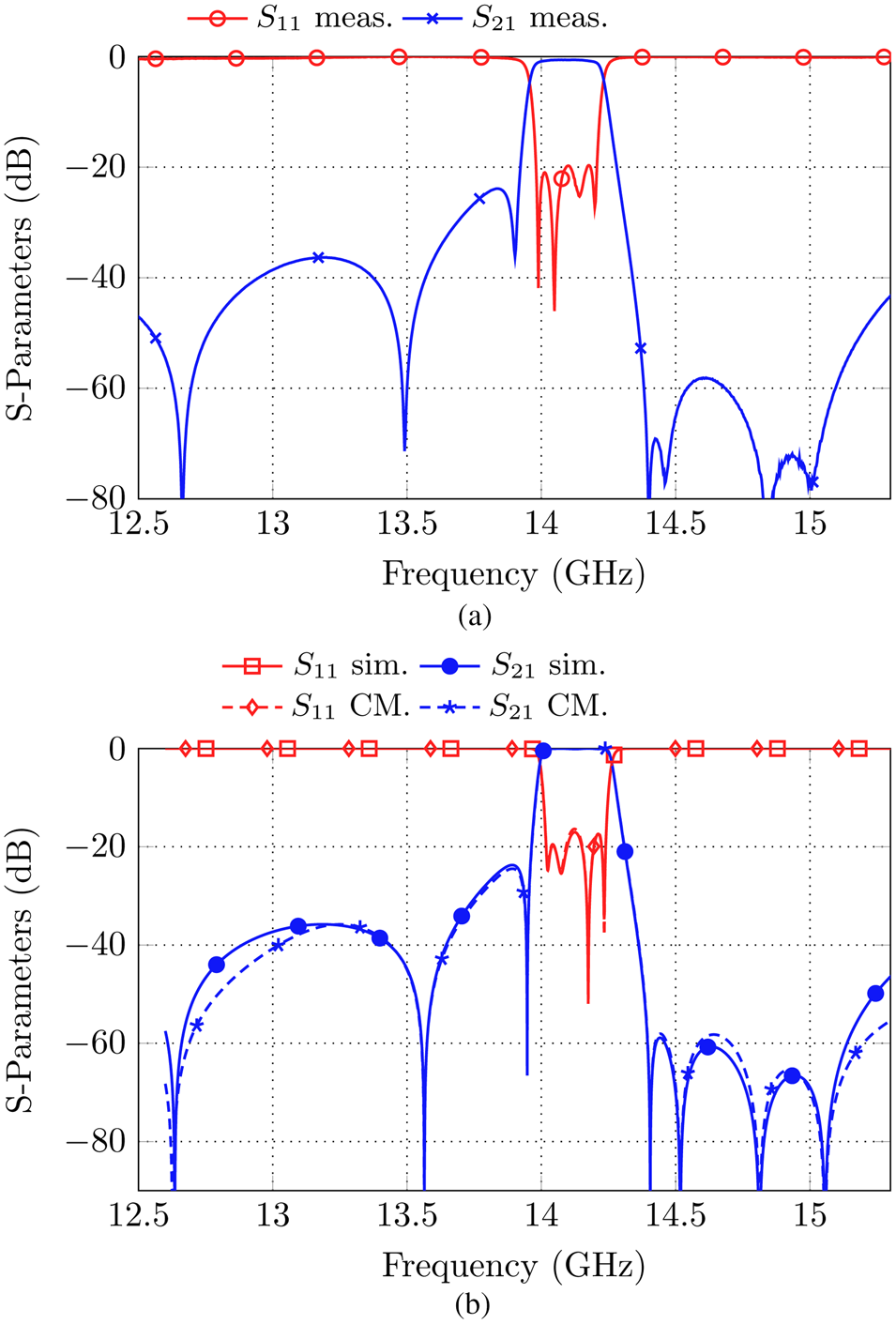
Fig. 4. (a) Measurement results of the filter set-up shown in Fig. 1(a) with additional source to load cross-coupling (with parameters s 0 = 31.8 and d SL = 5.6) [Reference Miek, Morán-López, Ruiz-Cruz and Höft13], (b) comparison of the simulated S-parameters with the coupling matrix in (2).
It is furthermore possible to find a coupling matrix description even for the improved design based on the coupling diagram proposed in [Reference Mokhtaari, Bornemann, Rambabu and Amari12]. There, a source-load cross-coupled fourth-order dual-band filter with two extra TZs is investigated (in total six TZs arise). The extra TZs are modeled by two additional de-tuned resonators in the source/load port. In total, six resonators are necessary to model the near passband behavior and the six TZs correctly. A very similar approach with six resonators is used in the following section “Phase equalized filter with six TZs” to determine the coupling matrix of a fourth-order phase equalized filter with in total six TZs as well.

Nevertheless, in the case investigated here in total seven instead of six TZs are observed, therefore one more, i.e. three, de-tuned resonators are assumed between the source/load port based on the approach in [Reference Mokhtaari, Bornemann, Rambabu and Amari12]. Please note that in the case investigated here the number of TZs determines the number of nodes in the coupling matrix. n = 4 nodes are resonant while n fz − n = 3 nodes must be de-tuned. The reason can be found in the description of the S-parameters according to [Reference Cameron, Kudsia and Mansour1]:


where E(s) and F(s) are of degree n and P(s) is of degree n fz. The order of P(s) determines the number of TZs. However, as a filter is a passive system, the condition n ≥ n fz must be fulfilled. It is therefore required to add n fz − n de-tuned nodes to the coupling scheme. The proposed topology is shown in Fig. 5 with the corresponding coupling matrix in (2), which was found by optimization. As a starting point, the entries of the coupling matrix in Table 1 were used and all entries according to the coupling scheme in Fig. 5 are enabled for optimization. It is possible to fit the simulated S-parameter response over nearly the whole simulation range as shown in Fig. 4(b), where the simulation results are compared with the S-parameters generated from the coupling matrix. However, multiple couplings between the de-tuned resonators and the remaining nodes are necessary for a sufficient coupling matrix fit wherefore the physical clarity suffers. In the following section “Phase equalized filter with six TZs”, a more suitable coupling matrix and topology for a six TZ filter is proposed.
Phase equalized filter with six TZs
The filter set-up proposed in section “Basic filter set-up” (Fig. 1) can be used in different configurations. By changing the parameter s 1, which defines the position of the cross-coupling aperture between cavity one and four on the z-axis, a phase equalized filter might be realized by exploiting a complex pair of TZs. For relatively large values of s 1, it is obvious that destructive interference arises between the right magnetic circle of cavity one and the magnetic field in cavity four (compare Fig. 1(b)), realizing two real frequency axis TZs as proven by the measurements in Fig. 3. However, for small values of s 1, constructive interference between cavity one and four arises. In this case, the left magnetic circle in cavity one couples with the magnetic field in cavity four, implementing a coupling with equal sign as the main-line couplings. The filter of section “Basic filter set-up” was used as a starting point and the Trust Region Framework in CST Microwave Studio as well as coupling matrix extraction techniques are used to adapt the filter dimensions. Simulation results for a filter set-up without a direct source to load coupling show in total three TZs, two of which realize a complex pair while the real frequency axis TZ arises below the passband. However, for the direct source to load coupled filter set-up, a maximal number of six TZs can be reached. The simulated S-parameter response is shown in Fig. 6(a).

Fig. 5. Coupling diagram to fit the simulated S-parameters in Fig. 4 based on the description in [Reference Mokhtaari, Bornemann, Rambabu and Amari12].
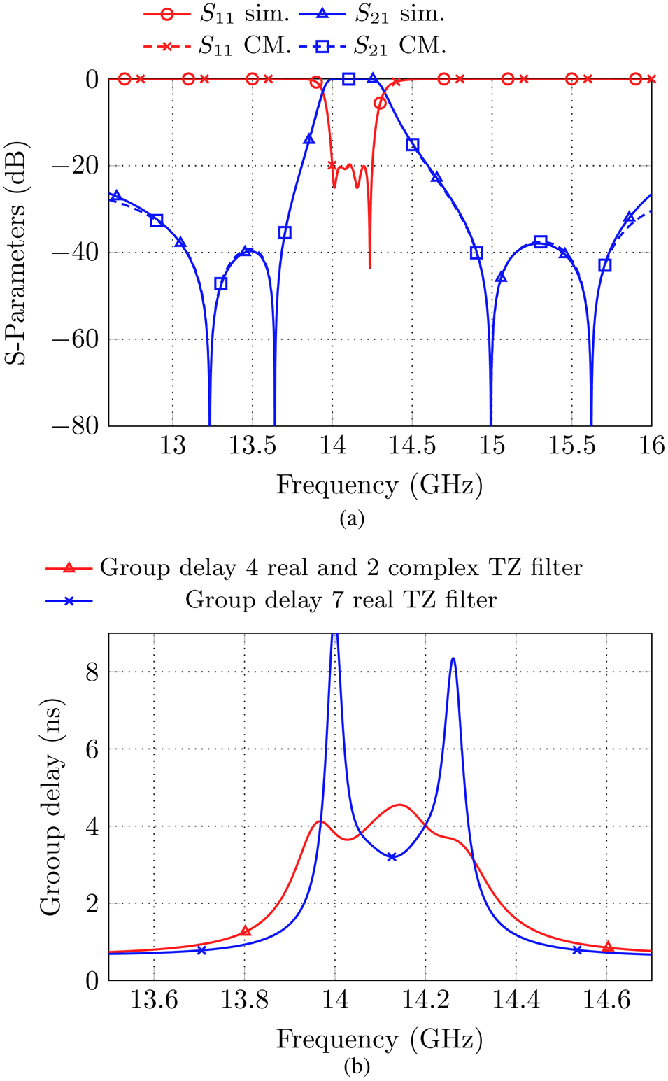
Fig. 6. (a) Simulated S-parameters in comparison to the S-parameters from the coupling matrix in (3) for the phase equalized fourth-order filter. (b) Comparison of the group-delay of the phase equalized filter and the 7 TZ filter from section “Basic filter set-up”.
The presence of a complex pair of TZs is proven by the relatively flat group delay compared to the filter with seven real frequency axis TZs, as shown in Fig. 6(b). The group delay variation within the passband is limited to less than 1 ns. The filter with seven real TZs shows a variation of roughly 5 ns from the passband center to the edge of the passband. The S-parameters of Fig. 6(a) are found for parameters s 0 = 5 mm, d SL = 8.25 mm, and s 1 = 8 mm. In the considered case, the physical source to load cross-coupling aperture is quite close to the cavities, which does not influence the footprint significantly.
A coupling matrix which fits the simulated S-parameter response might be found by adding two further de-tuned resonators close to the source/load port, similar to the approach in section “Basic filter set-up” [Reference Mokhtaari, Bornemann, Rambabu and Amari12]. These resonators account for the distance between the source and load port to the cross-coupling and are necessary to model the additional TZs. The coupling matrix to fit the adapted topology in Fig. 7 is shown in (3). A comparison of the S-parameters from simulation and the response from the coupling matrix is shown in Fig. 6(a) and shows very good agreement. The coupling matrix is again found by optimization, where the coupling matrix in Table 1 is used as a starting point. The resonators five and six are strongly de-tuned, which becomes obvious by observing the main-diagonal in (3). Nevertheless, this coupling matrix has a better physical clarity as there are less couplings necessary between resonator five/six and source/load or resonator one/two compared to the coupling matrix in (2).

Fig. 7. Coupling topology for the coupling matrix in (3).
Filter set-up with double source to load coupling
The aim of this section and the following one is to increase the total number of TZs provided by the filter set-up within the useful frequency region of the Ku-band. Two approaches are therefore investigated: in this section, the influence of a double-slotted source to load coupling on the number of TZs is examined, while in section “Filter set-up with additional frequency-dependent coupling structures”, additional frequency-dependent coupling structures are added to the physical filter set-up.
The basic filter structure investigated in this section is similar to the one proposed in Fig. 1(a) and is shown in Fig. 8 for the sake of clarity. Identical filter specifications are desired for an easy comparability among the set-ups. The additional TZs in section “Basic filter set-up” are mainly realized by the dispersive/resonant behavior of the source to load cross-coupling. Far away from the passband of the filter, standing waves arise due to the reflected energy from the first blend in the source/load port. These standing waves interfere constructively or destructively with each other, depending on the frequency as well as on the position and diameter of the source to load coupling. An empirical approach is therefore to add a further slot in the parallel source/load port for the realization of a double-slotted source to load coupling. The basic structure with parameters s 0,1 = 34.224 mm, s 0,2 = 6.693 mm, d SL,1 = 4.1 mm, and d SL,2 = 5.5 mm is shown in Fig. 8, while Fig. 9 shows a photo of the manufactured filter. To increase the Q-factor, the lower half as well as the cover were manufactured in aluminium. Tuning screws can be inserted at identical positions as in Fig. 1(b).
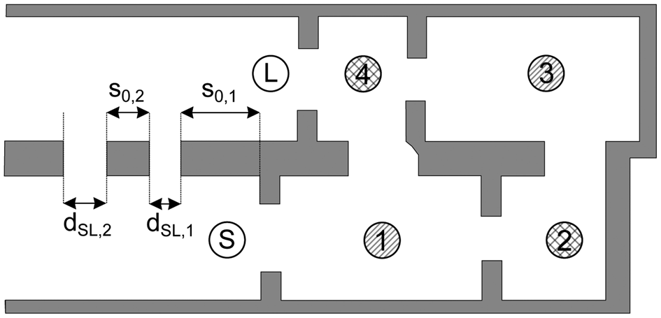
Fig. 8. Schematic view of the proposed filter set-up with a double-slotted source to load coupling.

Fig. 9. Manufactured filter with a double-slotted source to load coupling.
As can be seen in the measurement results in Fig. 10, in total eight TZs in the usable frequency region of the Ku-band can be realized. Above the passband, the appearance of the TZs is similar to the one in Fig. 4. Nevertheless, below the passband, four TZs are now generated as well. Compared to former measurements, the attenuation behavior above the passband is nearly identical but below the passband an improvement can be noticed. All in all, the measurement results show good agreement with the simulation and the position of all TZs is nearly as expected. The inset in Fig. 10 shows the insertion loss performance in the passband, which corresponds to a Q-factor of Q u ≈ 2700.

Fig. 10. S-parameter response of the manufactured filter from Fig. 9 in comparison to the simulation.
Filter set-up with additional frequency-dependent coupling structures
Filter set-up without source to load cross-coupling
The aim of the following investigation is to increase the number of available TZs of the basic Ku-band filter set-up from section “Basic filter set-up” by using frequency-dependent coupling structures. Different types of frequency-dependent couplings were investigated in the literature until now, e.g. [Reference Szydlowski, Lamecki and Mrozowski5–Reference Rosenberg, Amari and Seyfert8, Reference Szydlowski, Lamecki and Mrozowski21, Reference Rosenberg and Amari22]. The advantage of these structures is that TZs might be realized in an in-line configuration without requiring cross-couplings between non-adjacent cavities or extracted pole cavities. A commonly known structure of a frequency-dependent coupling aperture is a partial height post, as proposed the first time in [Reference Rosenberg and Amari22] for the application in band-stop filters. The utilization in in-line band-pass filter configurations was proven in [Reference Politi and Fossati7, Reference Szydlowski, Lamecki and Mrozowski21] while in [Reference Szydlowski, Lamecki and Mrozowski5] the application within a cross-coupling was proposed to increase the number of TZs generated by a quadruplet from two to three. However, the combination of frequency-dependent coupling structures with usual cross-couplings, bypass couplings as well as a direct source to load coupling was not investigated until now to the best of the authors knowledge.
The basic filter structure is similar to the one proposed in section “Basic filter set-up” (Fig. 1), where now the former inductive couplings between the source port and cavity one as well as cavity four and the load port are replaced by a partial height post, leading to the coupling diagram in Fig. 11(a) and the filter structure in (b). All couplings which are now realized by a frequency-dependent coupling are marked by an arrow. Please note that also the bypass couplings m S2 and m S4 become frequency-dependent by the insertion of a partial height post in the source port. Furthermore, the topology in Fig. 11(a) needs no additional de-tuned resonators as at this point the filter is investigated without a direct source to load cross-coupling. The presence of additional TZs can be modeled by the frequency-dependent couplings generated by the partial height posts.

Fig. 11. (a) Topology of the fourth-order Ku-band filter with frequency-dependent couplings between the source port and cavity one as well as cavity four and the load port and (b) position of the frequency-dependent posts in the overall filter set-up.
The basic structure of a post within a waveguide channel with all available degrees of freedom is shown in Fig. 12(a). The discrete equivalent circuit is shown in Fig. 12(b) and is identical to the one proposed in [Reference Szydlowski, Lamecki and Mrozowski23], where the partial height post was investigated in depth. A classical T-inverter is assumed where the series impedances Z 1 + Z 2 load the adjacent resonators. The frequency dependence of the coupling factor K can be calculated directly from the S-parameters, which are obtained by EM-simulations. Relation (6) can be obtained by equating the ABCD parameters of an ideal inverter with the ones generated by the equivalent circuit from Fig. 12(b).

Note that a phase de-embedding of the S-parameters to the center of the post is necessary for the evaluation of the equation above, implied by the length l deemb in Fig. 12(a).

Fig. 12. (a) Partial height post with height h, side-length t, and offset from the center position o c in a waveguide channel, (b) discrete equivalent circuit from [Reference Szydlowski, Lamecki and Mrozowski5].
It is assumed that the post in Fig. 12(a) has a square footprint of length t, a height h (which is smaller than the waveguide height b), and an offset from the center position o c. The basic dependencies of the coupling coefficient K from these parameters are shown in Figs. 13(a)–13(c). In Fig. 13(a), the footprint of the post is varied. Obviously, the position of the TZ generated by the post (indicated by the zero-crossing) is only minor affected whereas the coupling factor can be adapted by the parameter t. The position of the TZs might be adapted by the height h as well as the offset of the post o c, as shown in Figs. 13(b) and 13(c). Depending on both parameters, TZs above and below the passband can be realized.

Fig. 13. Parameter study of the post coupling structure for the variation of (a) the footprint (1 mm ≤ t ≤ 4 mm with fixed parameters h = 4.61 mm and o c = 5.13 mm), (b) the height (3.25 mm ≤ h ≤ 6.75 mm with fixed parameters t = 2.55 mm and o c = 5.13 mm) and (c) the offset from the center position (1 mm ≤ o c ≤ 6 mm with fixed parameters t = 2.55 mm and h = 4.61 mm).
For the realization of the coupling scheme in Fig. 11(a), a partial height post is inserted in the source port and a second one in the load port, replacing the former inductive irises. The design of the posts dimensions might follow the coupling matrix synthesis technique as proposed in [Reference Szydlowski, Lamecki and Mrozowski5, Reference Szydlowski, Leszczynska and Mrozowski24]. However, it is also possible to use the following procedure to find the physical dimensions of the posts with standard coupling matrix and optimization techniques:
(1) Based on the dependencies found in Fig. 13, the TZ generated from the post is shifted relatively far away from the passband by e.g. increasing the post height.
(2) As subsequently no TZ is generated from the post in the near vicinity of the passband, standard coupling matrix extraction techniques can be used for initial filter tuning, e.g. [Reference Macchiarella and Traina25].
(3) In the next step, the TZ is shifted step-by-step close to the passband at the desired position, where de-tuning effects might be compensated by optimization techniques in a full-wave simulator, e.g. the Trust Region Framework in CST Microwave Studio.
The standard design (without SL coupling) in Fig. 1 reveals three TZs, two of which above and one below the passband (compare also the measurement results in Fig. 3). Two TZs are now added below the passband by using the partial height posts. The post in the source port is designed to realize a TZ at 13.05 GHz, while the post in the load port reveals a TZ at 13.48 GHz. Dimensions as shown in Table 2 were found for the posts.
Table 2. Dimensions of the posts in the source/load port.

A coupling matrix description is possible if the frequency-dependent couplings are considered in e.g. the optimization procedure. The starting point is the well-known impedance matrix description of a coupled resonator filter given by [Reference Cameron, Kudsia and Mansour1]

with M1 is the classical (n + 2) × (n + 2) coupling matrix and s is the complex lowpass frequency variable. M2 is an identity matrix which accounts for the frequency dependence of the resonators and is therefore zero at positions (1, 1) and (n + 2, n + 2). The matrix R accounts for the resistive source and load terminations and has therefore entries only at position (1, 1) and (n + 2, n + 2). The frequency dependence of the couplings m S1, m S2, m S4 as well as m 4L can now be accommodated in matrix M2. For the generation of the impedance matrix (7), the coupling matrix in Table 1 is used as a starting point for the optimization and only the frequency-dependent entries in M2 are varied. To achieve a sufficient good fit between the simulation and the coupling matrix, all entries in M1 and M2 are optimized in a second step. The results are shown in Tables 3 and 4. Note, that the appearance of the frequency-independent coupling matrix in Table 3 is very similar to the one of the basic set-up as shown in Table 1. Figure 14 compares the simulated S-parameters of the filter set-up in Fig. 11 with the S-parameters from the coupling matrices from Tables 3 and 4. A very good agreement over nearly the whole frequency region is achieved. Furthermore, the dotted lines illustrate the frequency response of only the frequency-independent coupling matrix M 1. Three TZs are present, while the outer TZ is shifted to higher frequencies. However, if the frequency-dependent coupling matrix is taken into account as well, five TZs arise. The three TZs below the passband are realized by the partial height posts and by the cross-coupling of cavities one and four.

Fig. 14. Simulated S-parameters in comparison to the S-parameters generated by the coupling matrices.
Table 3. Coupling matrix M1 to fit the S-parameters in Fig. 14

Table 4. Coupling matrix M2 to fit the S-parameters in Fig. 14

As a proof of concept, the filter was manufactured in aluminum (AlMg3), as shown in Fig. 15. The direct source to load cross-coupling can be closed by a small brick and is therefore only used in the second measurement. The posts are very close to the side wall of the waveguide channel. It is therefore not possible to manufacture them in one piece with the waveguide filter due to milling issues. Hence, the posts are manufactured separately with a thread on the lower side. Holes are foreseen at the post position in the waveguide filter and after manufacturing all posts can be screwed at the desired positions.

Fig. 15. Manufactured fourth-order waveguide filter with frequency-dependent couplings in the source and load port for the realization of the coupling scheme in Fig. 11. The direct source to load coupling slot is closed by a small brick for the measurement results in section “Filter set-up without source to load cross-coupling” and only used for the measurements in section “Measurement set-up with additional source to load cross-coupling”.
The measured S-parameters in comparison to the simulation are shown in Fig. 16. The insertion loss in the passband is on average approximately 0.5 dB, which corresponds to a quality factor of Q u ≈ 3200.

Fig. 16. Measurement results in comparison to the simulation for the filter set-up with frequency-dependent couplings in the source and load port.
Measurement set-up with additional source to load cross-coupling
The filter in Fig. 15 is able to realize additional TZs by using the direct source to load cross-coupling. The aperture was positioned at s 0 = 44 mm and d SL = 5.45 mm. The position was found by parameter sweeps as an analytical calculation of the position to reproduce a certain TZ pattern is not possible until now. The S-parameter response is shown in Fig. 17, revealing very good agreement between measurement and simulation. A small frequency shift might by observed which occurs due to the chosen tuning state. Again, four TZs above the passband between 14.4 and 15 GHz very similar to the former measurements can be observed. In this frequency region, an attenuation of better than 60 dB can be reached. The TZ pattern below the passband differs from the one in Fig. 10. Two TZs very close to the passband realize a steep slope and two further TZs at 13.4 GHz as well as at 12.75 GHz can be observed. The attenuation behavior below the passband is better than 38 dB over the whole frequency region. The inset of the plot shows a close-up of the measured insertion-loss. Compared to the former measurements in Fig. 16, higher losses arise. A Q-factor of approximately Q u ≈ 2600 can be calculated. The reason for the lower Q-factor compared to the first measurement in Section “Filter set-up without source to load cross-coupling” might be that the screws for the cover were not pulled tight enough or an increasing oxide film reduces the electrical conductivity at the transitions between cover/bottom and the flanges.
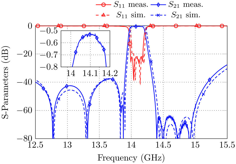
Fig. 17. Measurement results in comparison to the simulation for the filter set-up with frequency-dependent couplings in the source and load port with additional direct source to load cross-coupling.
Conclusion
In this paper, a fourth-order Ku-band filter for the realization of multiple TZs is investigated. Based on the initial design, which is able to realize seven TZs in the useful Ku-band frequency range, three additional set-ups are investigated in this paper. The first set-up shows the versatility of the proposed configuration as by small changes a phase-equalized filter can be implemented. This filter is able to realize in total up to six TZs, while two of which are complex. Eight real frequency axis TZs can be realized by a similar filter with double slotted source to load cross-coupling. Finally, frequency-dependent couplings are added to the basic filter set-up. As a result, five TZs are obtained for the set-up without an SL coupling while again eight TZs are realized by the set-up with SL coupling. Three simulation results were proven by measurements, which show very good agreement with the simulation over nearly the whole frequency band. Furthermore, two coupling matrices to model the filter with six and seven TZs are derived and a frequency-dependent coupling matrix to model a five TZ filter set-up is proposed.
Acknowledgements
The authors would like to thank M. Mrozowski and A. Lamecki for valuable discussion about frequency-dependent coupling apertures.
 Daniel Miek received the B.Sc. and M.Sc degrees in electrical engineering and information technology from the University of Kiel, Kiel, Germany in 2015 and 2017, respectively, where he is currently pursuing the Dr.-Ing. degree as a member of the Chair of Microwave Engineering with the Institute of Electrical Engineering and Information Technology. His current research interest includes the design, realization, and optimization of microwave filters as well as parameter extraction and computer-aided tuning.
 Patrick Boe received the B.Sc. and M.Sc. degrees in electrical engineering, information technology and business management from Kiel University, Kiel, Germany, in 2017 and 2019, respectively. Currently he is pursuing the Dr.-Ing. degree as a member of the Chair of Microwave Engineering with the Institute of Electrical Engineering and Information Technology. His current research interest includes the design, realization, and optimization of dielectric resonator filters as well as dielectric multi-mode filters.
 Fynn Kamrath received the B.Sc. and M.Sc. degrees in electrical engineering and information technology from Kiel University, Kiel, Germany in 2017 and 2019, respectively. Currently he is pursuing the Dr.-Ing. degree as a member of the Chair of Microwave Engineering with the Institute of Electrical Engineering and Information Technology. His current research interests include the design, realization, and optimization of center frequency and bandwidth tunable microwave filters in the Ka-Band.
 Michael Höft was born in Lübeck, Germany, in 1972. He received the Dipl.-Ing. degree in electrical engineering and Dr.-Ing. degree from the Hamburg University of Technology, Hamburg, Germany, in 1997 and 2002, respectively. From 2002 to 2013, he joined the Communications Laboratory, European Technology Center, Panasonic Industrial Devices Europe GmbH, Lüneburg, Germany. He was a Research Engineer and then Team Leader, where he had been engaged in research and development of microwave circuitry and components, particularly filters for cellular radio communications. From 2010 to 2013, he had also been a Group Leader for research and development of sensor and network devices. Since October 2013 he is a Full Professor at the Kiel University, Kiel, Germany in the Faculty of Engineering, where he is the Head of the Microwave Group of the Institute of Electrical and Information Engineering. His research interests include active and passive microwave components, (sub-) millimeter-wave quasi-optical techniques, and circuitry, microwave, and field measurement techniques, microwave filters, microwave sensors, as well as magnetic field sensors. Dr. Höft is a member of the European Microwave Association (EuMA), the association of German Engineers (VDI), a member of the German Institute of Electrical Engineers (VDE), and a senior member of IEEE.


 Open access