


1. Introduction
In the last three to five years, brands and retailers have begun aggressive marketing campaigns for sustainable products due in large part to consumers becoming increasingly environmentally conscious. Best and Mitchell (Reference Best and Mitchell2018) found that brands and retailers are shifting their focus to marketing sustainable products to a more environmentally cognizant generation that desires products aligning with their values. This has put additional pressure on the cotton industry to document field-level practices to ensure sustainable practices were used throughout the production process. Sustainable Development Goals, which have replaced Millennial Development Goals, encompass 17 goals, each with multiple underlying targets and associated data indicators that are to be achieved by 2030. These goals are predicted to incorporate $5 to $7 trillion around the world each year to achieve desired sustainability goals over a 15-year period between 2015 and 2030 (Vorisek and Yu, Reference Vorisek and Yu2020). According to Mkele (Reference Mkele2018), sustainable attributes are becoming a more essential component of agricultural products as consumers are becoming more conscious towards the environment around them. These trends are causing agricultural producers to face an increasing demand to benchmark sustainable practices at the field level.
The general concept of agricultural sustainability, originally outlined in the Brundtland Report is built upon three basic pillars: economic viability, social equitability, and friendliness towards the environment (WCED, 1987; Hansmann, Mieg, and Frischknecht, Reference Hansmann, Mieg and Frischknecht2012). To ensure that sustainability is obtained and maintained in these three categories within the agricultural sector, WCED (1987) concluded that humanity must ensure that it meets the needs of the present without compromising the productivity of future generations. The lack of clear, defining characteristics for agricultural sustainability presents an issue for the diverse production occurring in the agricultural sector. Though maintaining economic viability and reducing environmental degradation seem to present clear goals for sustainable agricultural production, what actually accomplishes these objectives is very nuanced among producers. Also, research has proposed that accurately portraying the complex reality of agriculture’s impact on the environment and framing agricultural sustainability from a conceptual perspective is necessary for further development going forward (Janker and Mann, Reference Janker and Mann2020).
Changing consumer preferences has created world-wide demand for sustainably produced cotton and has put added pressure on U.S. cotton growers to document their farm practices. As a combination of science and marketing begin to play an increasingly critical role in how society views food and fiber products, there is a need for upcoming generations to find common ground with agricultural producers regarding sustainability. The desire to provide economic, environmental, and social equitability is constantly increasing throughout agricultural supply chains (Saitone and Sexton, Reference Saitone and Sexton2017). Because of this, producers find themselves living and working within standards set by consumer demands of sustainably produced goods. Sustainability is a relatively new criterion that most farmers, ranchers, and other agricultural producers will have to satisfy as consumer market power slowly shifts to more environmentally mindful generations. Over 75% of Brazilian cotton is BCI certified as sustainably produced, and 23% of the total global cotton supply is BCI certified, creating a differentiated cotton product in the market (BCI, 2020). To compete with BCI and to increase U.S. international competitiveness, the U.S. Cotton Trust Protocol was developed to provide farmers with a framework to create standards for continuous improvement throughout the supply chain; however, adoption among growers has been low.
There are tradeoffs to be made in the adoption of sustainable practices for both the consumer and producer as a new equilibrium is established for sustainable agricultural goods (Risbey et al., Reference Risbey, Kandlikar, Dowlatabadi and Graetz1999). Singh, Singh, and Singh (Reference Singh, Singh and Singh2015) show that producers’ awareness and skill sets should be altered to minimize losses in yield and maximize revenue to sustain future productivity in the agricultural sector that is shifting more importance towards sustainability. Assessing sustainability in agriculture has generally focused on environmental and technical issues in the past while neglecting economic and social aspects, the multifunctionality of agriculture, and the application of past results which has served as a hindrance for further development (Binder, Feola, and Steinberger, Reference Binder, Feola and Steinberger2010).
Developing a framework to quantify sustainability in agricultural production will help ensure the rebalancing of market power for all producers, consumers, and marketers within the supply chain. Van Passel et al. (Reference Van Passel, Nevens, Mathijs and Huylenbroeck2007) highlights the importance of establishing sustainable benchmarks to compare farmer-provided data to measure sustainable efficiency, which helps combine the sustainable use of natural resources with strong economic performance. The goal is not to create a perfect method to measure sustainability but to set industry-wide standards that generally apply to all crops to increase and encourage environmental stewardship in the agricultural supply chain (Sabiha et al., Reference Sabiha, Salim, Rahmanand. and Rola-Rubzen2016). The lack of valid and reliable indices to accurately quantify agricultural sustainability is a significant issue for the agricultural sector and further obstructs producers from implementing sustainable practices (Valizadeh and Hayati, Reference Valizadeh and Hayati2021). In addition, the development of these indicators could encourage consumer participation in furthering sustainable agricultural development to help foster comradery between producers and consumers (Hayati, Ranjbar, and Karami, Reference Hayati, Ranjbar and Karaami2010).
The objectives of this research were (1) to estimate producer willingness to accept (WTA) across preferred incentive categories for participating in sustainability programs, which includes providing information regarding management practices, financial aspects related to growing season, and other various aspects of growing practices to fulfill data requirements, as well as incentive amounts, (2) to evaluate WTA values for implementing sustainable practices, and (3) to analyze producers’ socio-demographic effects on WTP values for sustainability program attributes.
2. Materials and methods
The data for this research was collected through an online survey administered through Qualtrics in both Texas and Oklahoma. To increase survey response, over 200 producers, gins, cooperatives, and mills were called and visited to encourage participation, and survey participants were administered an Amazon e-gift card for $25.00. The survey was designed using a discrete choice framework while also incorporating both double-bounded contingent valuation (DBCV) questions and choice-based conjoint analyses to assess producer WTA. The SAS (SAS Institute, 2024) and STATA (StataCorp, 2023) code used in the following analysis is available upon request.
Discrete choice models have routinely been used to describe the relationship of decision maker’s choices when facing varying alternatives, and the contingent valuation method uses nonmarket valuations procedures to show variations from what can be interpreted as ‘common.’ Also, the double-bounded contingent valuations method builds upon the single-bounded method to increase the efficiency of both willingness to pay (WTP) and WTA measurements (Hanemann, Loomis, and Kanninen, Reference Hanemann, Loomis and Kannine1991).
The survey was conducted from August 1 to October 1 during 2021 after receiving approval from both the Texas Tech University Human Research Protection Program Institutional Review Board. Special precautions regarding COVID-19 were also taken when visiting various agricultural establishments to encourage participation. Achieving large sample sizes is challenging when conducting surveys with agricultural producers due to issues such as internet connectivity, time constraints, and sociodemographic characteristics of the respondents themselves (National Research Council, 2008; Ulrich-Schad et al., Reference Ulrich-Schad, Li, Arbuckle, Avemegah, Brasier, Burnham, Kumar Chaudhary, Eaton, Gu, Haigh, Jackson-Smith, Metcalf, Pradhananga, Prokopy, Sanderson, Wade and Wilke2022). Although there is not a general recommendation for the size of a sample, an n ≥ 30 is enough to satisfy the central limit theorem across many practical research applications (Montgomery and Runger, Reference Montgomery and Runger2011; Piepho et al., Reference Piepho, Gabriel, Hartung, Büchse, Grosse, Kurz, Laidig, Michel, Proctor, Sedlmeier, Toppel and Wittenburg2022). In total, 220 surveys were completed by producers with 160 used in the analysis after removing incomplete responses.Footnote 1
The first section of the survey obtained sociodemographic characteristics of producers including farming background and operation-specific information. This was followed by a section used to collect information of grower knowledge, attitudes, and perceptions towards sustainability and sustainability programs. The third part incorporated the double-bounded contingent valuation questions to evoke what monetary value producers would be willing to accept of a per acre basis to adopt a sustainable practice. This was followed by the choice-based conjoint analyses posed specifically to cotton producers to find their WTA for various incentives, prices, incentive combinations, and tradeoffs for cotton growers. Finally, the fifth section included a brief statement thanking the producers for their participation and an anonymous link for participants to enter their name and email address so they could subsequently be sent an Amazon e-gift card. In total, there were five survey versions that were randomly administered to respondents. Again, after pretesting snowball recruiting was used to reach producers through agricultural gins, mills, co-ops, and through direct contact with farmers.
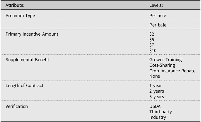
Since the cotton industry has been routinely advocating for the adoption of sustainability programs among producers and the potential of exogenous factors associated with other crops, the choice-experiments were only presented to cotton producers. Table 1 presents the attribute list with the different levels for each attribute. The premium was offered on either a per acre or per bale basis, and two separate models were created to interpret each premium level. The primary incentive amount is the level of premium the producer would be offered on a per acre or per bale contract. The $2.00 per bale premium offered by BASF’s e3 sustainability program was used as the base price for each contract type with three higher premium amounts of $5, $7, and $10. Higher premiums were included because of low participation rates and evidence from previous literature revealing that $2.00 is too low a premium amount. Supplemental benefits represent an offer of additional incentives in addition to the primary incentive amount, and the contract length, which varied from one to three years. Contract lengths can very considerably. In this case, short-term contracting lengths were used due to uncertainties with incentive amounts and program longevity (MacDonald et al., Reference MacDonald, Perry, Ahearn, Banker, Chambers, Dimitri, Key, Nelsen and Southard2004.) Also, most sustainability programs currently require third-party field-level verification so participants were presented with an option of who would potentially conduct field inspections with the assumption of no cost to the grower (U.S. Cotton Trust Protocol, 2024).
Table 1. Levels of attributes for the choice sets
For the DBCV questions in the survey, the objective was to find the minimum amount producers would be willing to accept per bale in order to adopt and incorporate sustainable practices into their operations. Figure 1 presents the flow of the DBCV question presented in the survey. Initially, producers were offered a bid amount of $5/bale, if they answered “yes” to the initial bid the bid amount was lowered to $2.50/bale. If the respondent answered “no” to the initial bid, they were presented with a higher bid amount of $10/bale.
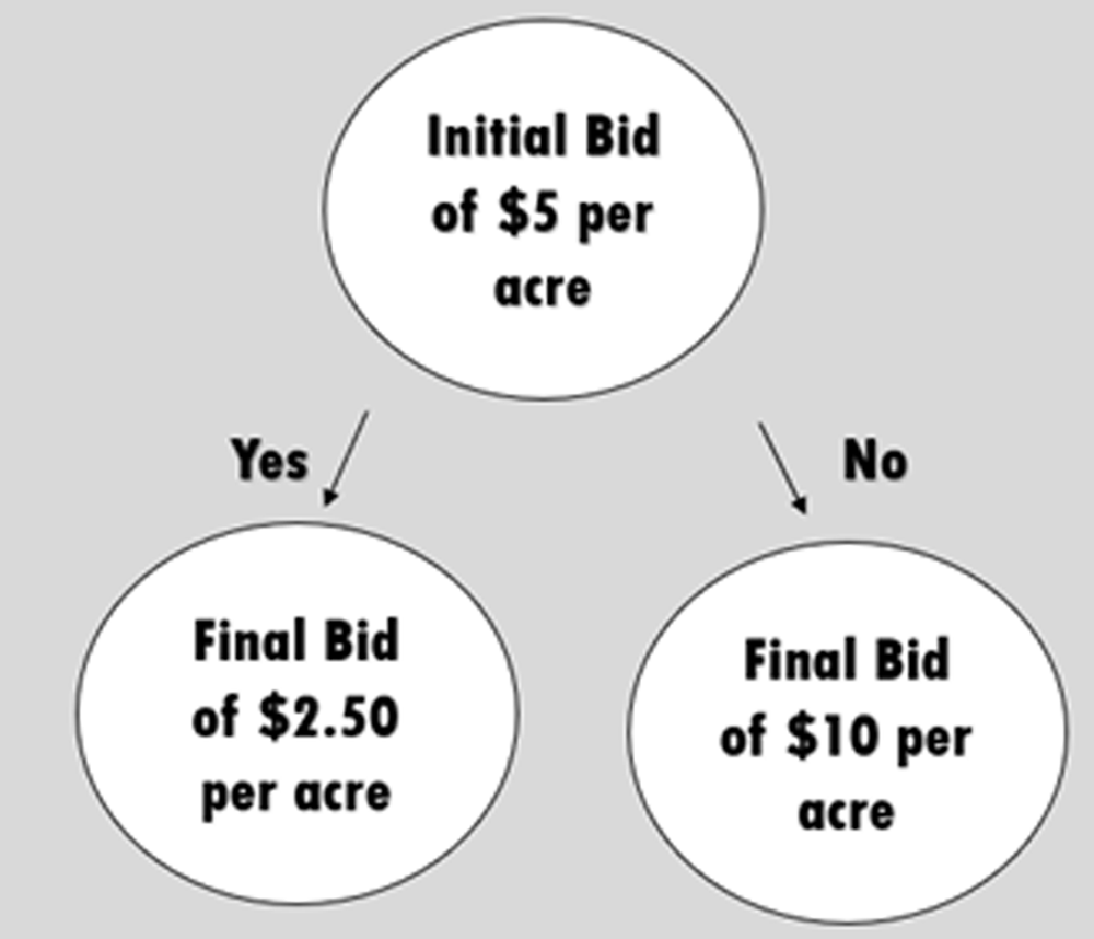
Figure 1. Double-bounded contingent valuation question flow.
The model used to estimate producer WTA in this study is based upon Lancaster’s (Reference Lancaster1966) demand theory regarding characteristics or attributes of the product and the random utility model (McFadden, Reference McFadden and McFadden1972). Following Lancaster (Reference Lancaster1966), instead of consumers having preferences for individual products, the growers’ preference for specific sustainability program attributes. Therefore, growers choose the program with a particular bundle of attributes that will maximize their utility subject to a budget constraint. In this study, the bundle of attributes is premium type, primary incentive amount, supplemental benefits, length of contract, and verification.
To estimate the parameters of the grower’s utility function, the probability of grower n to pick product l in choice scenario t, conditional on the coefficient vector θ n = [y n w ′ n ], is:
 $$P_{nlt}\left(\theta _{n}\right)=(e^{{V_{nlt\left(\theta _{n}\right)}}})/(\Sigma _{l}e^{{V_{nlt\left(\theta _{n}\right)}}})$$
where V nlt = − γ n p nlt + (γ n w n )′x nlt (Revelt and Train, Reference Revelt and Train1998). Conditional on ϴ n , the probability of grower n′s noted series of L choices is conveyed as:
 $${R_n}\left( {{\theta _n}} \right) = {\Pi _l}{p_{nt\left( {n,l} \right)l}}\left( {{\theta _n}} \right),$$
where t(n,l) denotes a specific product l that grower n selects in choice scenario t (Train, Reference Train1998). θ n is a coefficient vector and is unobserved for every grower n and varies through the population with density g(θ_n ∣ Γ), where the parameters of the distribution of θ_n are Γ. Therefore, the mixed logit (unconditional) choice probability of the observed choice sequence is:
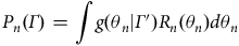 $${P_n}(\Gamma ) = \int g ({\theta _n}|\Gamma '){R_n}({\theta _n})d{\theta _n}$$
The log-likelihood function for grower n is:
 $$LL(\Gamma ) = {\Sigma _n}in\,{{\rm{P}}_n}(\Gamma )$$
The population density parameters, Γ, were found by using simulated maximum likelihood procedures in STATA (Rigby and Burton, Reference Rigby and Burton2006; Train, Reference Train1998). With respect to the distribution of the coefficients in θ n , the price coefficients are specified as lognormal, and the WTA distributions for non-price attributes are assumed to be normal.
The estimation of each individual grower’s WTA values is found through an application of Bayes’ rule. Because the density of θ n relies on the parameter vector for each individual’s choice sequence, it is as:
 $$f({\theta _n}|\Gamma ) = (g({\theta _n}|\Gamma ){R_n}({\theta _n}))/({P_n}(\Gamma ))$$
and the expected value of θ n is given by:
 $$E({\theta _n}|\Gamma ) = \int {} {\theta _n}{\rm{ }}f({\theta _n}|\Gamma )$$
which can be estimated using simulations:
 $$\widehat E({\theta _n})|\Gamma ) = ({\Sigma _d}{\theta ^d}{R_n}({\theta ^d}))/({\Sigma _d}{R_n}({\theta ^d})),$$
where θ d corresponds to the d-th draw from the population density g(θ n ∣ Γ), and R n (θ d ) is the probability of individual n’s sequence of choices (Revelt and Train, Reference Revelt and Train1998). Estimated parameters Γ 𐇤 are used in place of the parameters Γ𐇤 (Hess, Reference Hess2007). The stability of the estimated E𐇤(θ n ∣ Γ) values were verified using various sample draws.
Following this, a random effects panel regression model for the grower-related attributes are estimated:
 $$WTA_{nc}=t_{c}+y'_{n}b+h_{i}+u_{nc}$$
Where WTA nc is the nth grower’s WTA for each attribute, t c and b are coefficients, y n is a vector of grower-specific characteristics, h i is grower-specific random error, and u nc is the error term (Campbell, Reference Campbell2007). This approach provides estimates of the marginal effects of the growers’ related characteristics (knowledge, use, and perceptions and socio-demographic characteristics) on average WTA values for the attributes (Campbell, Reference Campbell2007).
Parametric and nonparametric methods were used for the DBCV estimations. The parametric approach for estimation uses parametric forms for the choice probabilities corresponding to the components of the equation (López-Feldman, Reference López-Feldman2012; Zapata et al., Reference Zapata, Carpio, Isengildina-Massa and Lamie2013). The probability that a respondent i answers “yes” to the first bid and “yes” to the second bid (Pr yy i ) is:
 $${Pr^{yy}}_{i}=\Pr \left({WTA_{i}}\leq PL_{i}\right)=G(PL_{i},\theta ),$$
in which G(., θ) is a parametric statistical cumulative density function with parameters θ. The probability that a respondent answers “yes” to the first bid and “no” to the second bid Pr yn i is:
 $${Pr^{yn}}_{i}=\Pr \left(PI_{i}\leq WTA_{i}\lt PL_{i}\right)=G\left(PI_{i},\theta \right)- G\left(PL_{i},\theta \right).$$
Similarly, the probability that a respondent answers “no” to the first bid and “yes” to the second bid Pr ny i is:
 $${Pr^{ny}}_{i}=\Pr \left(PI_{i}\lt WTA_{i}\leq PH_{i}\right)=G\left(PH_{i},\theta \right)-G\left(PI_{i},\theta \right).$$
Finally, the probability that a respondent answers “no” to both bids Pr nn i is:
 $${Pr^{nn}}_{i}=\Pr \left(PH_{i}\lt WTA_{i}\right)=1-G(PH_{i},\theta ).$$
Given a sample of N individuals, the log-likelihood becomes:
 $$\eqalign{L& =\Sigma _{i=1}^{N}d_{i}^{y_{i}^{1}=1y_{i}^{2}=0}\ln \left(G\left(PI_{i}, \theta \right)-G\left(PL_{i},\theta \right)\right)+d_{i}^{y_{i}^{1}=1y_{i}^{2}=1}\ln \left(G\left(PL_{i}, \theta \right)\right)\cr& \quad+d_{i}^{y_{i}^{1}=0y_{i}^{2}=1}\ln \left(G\left(PH_{i}, \theta \right)-G\left(PI_{i},\theta \right)\right)+d_{i}^{y_{i}^{1}=0y_{i}^{2}=0}\ln \left(1-G\left(PH_{i},\theta \right)\right),}$$
in which d i indicates the individuals belonging to the ith bidding process outcome, and y i 1 and y i 2 are used to denote the responses (1 = Yes or 2 = No) to the first and second binary choice questions, respectively (Cameron, Reference Cameron1988). Estimation of the parameters in the log-likelihood equation requires the assumption of a specific distributional form for G(., θ). In total, five statistical distributions were considered (normal, Weibull, log-normal, exponential, and log-logistic). The “best” model was selected using the Akaike information criterion, and the ratio of the maximum likelihood method proposed (Cameron and Trivedi, Reference Cameron and Trivedi2005; Raqab, Al-Awadhi, and Kundu, Reference Raqab, Al-Awadhi and Kundu2018).
Explanatory variables can also be introduced into the procedure by modeling some components of the parameter vector θ as a function of the explanatory variables. For example, the log-normal distribution is defined by two parameters (µ and σ); thus µ = X ′ i β, in which X ′ i is the vector of explanatory variables.
3. Results
3.1. Summary of sociodemographic characteristics
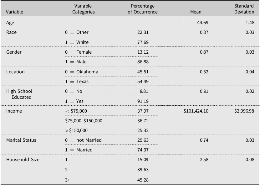
Table 2 shows the summary of statistics for the sociodemographic variables included in the analysis. The average age of respondents was 45 years old and 77.69% of respondents identifying as white. Notably, 13.12% of respondents were female despite the lack of attention women typically receive as a production partner or the lead-decision maker in agricultural operations (Joyce and Leadley, Reference Joyce and Leadley1977). Producers were evenly split between Oklahoma and Texas with 45.51% and 55.49% operating in each state, respectively. Farm size varied from 20,000 acres or less (65%), 2,000 to 5,000 acres (26%), 5,000 to 7,500 acres (6%), and greater than 7,500 acres (3%). For all respondents, 91.19% received at least a high school diploma and 74.37% were married. Also, average income was just over $100,000, which is above the average household income reported by the Bureau of Economic Analysis for 2021, and average household size was 2.58 including the lead decision-maker.
Table 2. Summary of sociodemographic variables for survey respondents
3.2. Summary of understanding and knowledge of sustainability
Respondents were asked to self-identify their level of understanding of sustainability on a five point likert scale, and 36.25% indicated they understood sustainability a moderate amount, 31.25% said a lot, 24.38% said a great deal, and 8.12% said a little or none at all. When asked about mandatory implementation of sustainable practices in the future, 40% said they might or might not be forced, 36.88% said probably yes, 11.88% said definitely yes, and 11.24% said probably no or definitely no. Also, all but one producer indicated they already implement at least one sustainable practice with the majority implementing crop rotation, cover crops, or no-till either separately or in conjunction with one another.
Regarding the three pillars of agricultural sustainability, producers were asked which category was the toughest to achieve with 74.84% choosing economic viability, 15.09% said social equitability, and 10.07% choosing friendliness towards the environment. The majority of respondents choosing economic viability is similar to results from previous research where 40% of farmers were found to be driven primarily by monetary goals (Ridley, Reference Ridley2004). Because one goal of this research was to increase producer participation in sustainability programs, one survey question asked if respondents were currently enrolled in such a program that encouraged sustainable behavior. Only 17.5% of respondents were currently enrolled in a sustainability program with 50% of those having neutral feelings towards the program, and the majority of producers not enrolled in a program indicated that it being a time-consuming process and the fear of their information being used against them as reasoning for not participating.
Producers were also asked what their main cash crop was with 34.59% selecting cotton, 33.96% wheat, 12.58% soybeans, 8.81% “other,” 6.29% corn, and 3.77% selecting sorghum. The average total acres farmed was 2,370.68 per farmer, and 48.75% of producers said they do not sell through a cooperative. Regarding employment, 50.62% indicated farming was their full-time job with the majority of producers (53.55%) farming greater than sixteen years, and 73.77% were at least a third-generation farmer.
3.3. Mixed logit results
The mixed logit model results are presented in Table 3, where Model 1 uses the per acre payout and Model 2 incorporates the same attributes but uses the per bale premium amount. Average WTA amounts for each contract type are calculated from the ratio of ASC to incentive amount for each payout type. The average values that producers would accept for enrolling in a sustainability program under the per acre and per bale contract are $16.84 and $4.93, respectively. These average values are the baseline WTA amounts for each payout type when no other attributes are considered. From the initial mixed logit results, the coefficients for each attribute do not have direct interpretation but are used for further analysis subsequently.
Table 3. Mixed logit estimation results for Model 1 and Model 2
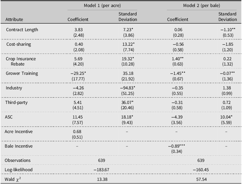
Notes: Panel Mixed Logit model using 100 Halton draws to maximize producers’ utilities in both models (Zeng, Reference Zeng2016). Attributes assigned a normal distribution with the exception of acre incentive that was designed to follow a lognormal distribution. ASC represents the alternative specific constant.
***indicates significance at 1% level, **indicates significance at 5%, and *indicates significance at 10%.
Values in parentheses indicate the standard error of the coefficient.
Tables 4 and 5 present the estimated marginal WTA values obtained from the mixed logit results in Table 3, respectively. Negative amounts are interpreted as the monetary values producers are willing to accept while positive amounts are the values they are willing to give up for enrolling in a sustainability program relative to the baseline. Negative signs indicate an increase in overall contract payment while positive signs show a decrease in overall contract payout. From here, willingness to pay (WTP) is used to show the monetary values producers would be willing to pay to not participate in such a program, or deviation from the minimum value producers require for participation. For the supplemental benefits attribute, the baseline was none and for verification the baseline was government (i.e., USDA).
Table 4. Estimated marginal willingness to accept estimates ($/acre) in Model 1
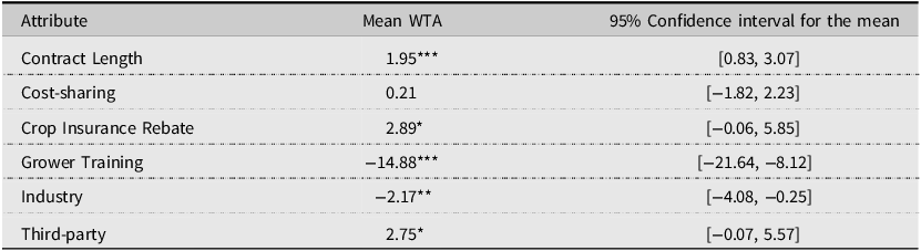
Notes: β represents the attribute’s mean coefficient estimated in equation (5).
***Indicates significance at 1% level, ** indicates significance at 5%, and * indicates significance at 10%.
Carson and Czajkowski (Reference Carson and Czajkowski2019), when the price attribute follows a lognormal distribution and constraining the standard deviation of price to 0 and other variables all follow a normal distribution to obtain the mean WTA values.
95% confidence intervals were found using Fieller (Reference Fieller1954) method.
Table 5. Estimated marginal willingness to accept estimates ($/bale) in Model 2
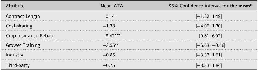
Notes: β represents the attribute’s mean coefficient estimated in equation (5).
***indicates significance at 1% level and **indicates significance at 5% level.
Carson and Czajkowski (Reference Carson and Czajkowski2019), when price attribute follows a lognormal distribution and constraining the standard deviation of price to 0 and other variables all follow a normal distribution to obtain the mean WTA values.
95% confidence intervals were found using Fieller (Reference Fieller1954) method.
The positive values in Table 4 show that producers are willing to decrease the price of their overall contract for an increase in contract length, to have cost-sharing or a crop insurance rebate as the supplemental benefit, and to have a third-party as the verification entity. On average, WTP for both contract length and crop insurance rebate as the supplemental benefit were statistically significant and were $1.95 per acre and $2.89 per acre, respectively. Additionally, producers were willing to accept an average of $14.88 per acre for grower training as the supplemental benefit, compared to no supplemental benefit. Moreover, producers were willing to accept, on average, $2.17 per acre for industry as the verification entity, compared to USDA verification. These results are consistent with previous research showing that both the length of a sustainability contract and trust association with verification entity have a significant impact on whether farmers would enroll in a hypothetical contract (Arifin et al., Reference Arifin, Swallow, Suyanto and Coe2009; Jin, Bluemling, and Mol, Reference Jin, Bluemling and Mo2015).
Table 5 shows the estimated marginal WTA values for the per bale contract calculated using the marginal effects from the mixed logit results. With the per bale contract, farmers were willing to pay, on average, $0.14 per bale as the length of the contract increases. For the supplemental benefits, producers were willing to pay, on average, $3.42 per bale for a crop insurance rebate, compared to no benefit. However, producers were willing to accept an average of $1.38 and $3.55 for cost-sharing and grower training as the supplemental benefits, compared to none benefit, respectively. Also, they were willing to accept $0.85 and $0.75 for industry and third-party verification, compared to USDA verification, respectively.
3.4. Effects of sociodemographic characteristics on WTA
Following the previous marginal analyses, random effect regression models were estimated to identify the relationships between WTA for sustainability program contracts on a per acre and per bale basis, producer demographic characteristics, and operational specifics. For each contract type, three random effects regression models were estimated. The random effects models include WTA values for contract length, verification entity with industry as the baseline, and supplemental benefits with cost-sharing as the baseline attribute.
Table 6 presents the random effects model results for the per acre models. The results show that producers were willing to accept, on average, $0.19 and $0.06 more per acre for a crop insurance rebate and grower training compared to the baseline of cost sharing as the supplemental benefit, respectively. Compared to the baseline of industry verification, producers were willing to pay $0.34 more per acre for third-party verification.
Table 6. Random effect regression models for acre incentives

Note: ***indicates significance at 1% level, **indicates significance at 5%, and * indicates significance at 10%.
Regarding the included producers’ demographic characteristics (age, race, gender, and education), only producers’ gender was found to be statistically significant for all three regressions. Specifically, male producers were willing to accept $2.54, $28.20, and $3.06 more per acre, compared to their female counterparts, for the contract length attribute, the verification entity attribute, and supplemental benefit attribute, respectively. For the Contract Length regression, each year increase in age was associated with a $0.04 increase in producers WTA values for the contract length attribute. For the same regression, producers identifying as White had a higher WTA of $2.55 per acre for the contract length attribute, compared to producers identifying as a different race. Also, in the contract length regression, producers currently enrolled in a sustainability program were willing to pay $1.19 per acre for the contract length attribute, compared to those not currently enrolled in such a program. For the verification entity regression, producers identifying as white had a higher WTA compared to other races of $15.32 per acre for the verification attribute. Finally, in the supplemental benefits regression a one-year increase in age increased WTA for the supplemental benefit attribute, by $0.05 per acre.
Table 7 shows the results for the random effects regressions for the per bale model. The regressions were constructed in the manner and included the same variables as the per acre model. For the supplemental benefits regression, producers were willing to accept $23.59 per bale for crop insurance rebate and were willing to pay $97.08 per bale for grower training as the supplemental benefit compared to the baseline of cost sharing. For verification entity, producers were willing to accept $4.58 per bale for third-party verification compared to industry as the verification entity. None of the included demographic variables exhibited statistical significance across all three regressions but they were all statistically significant, with the exception of producers’ age, race and gender, in the regression for contract length. Specifically, each additional year age is associated with a $0.01 per bale increase in WTA values for the contract length attribute. Producers identifying as White were willing to accept, on average $1.15 per bale more for the contract length attribute relative to producers identifying as a different race. Male producers had higher WTA values, on average, $1.46 per bale relative to female producers for the contract length attribute. Also, producers currently enrolled in a sustainability program were willing to pay $0.92 per bale more than producers not enrolled in such a program for the contract length attribute.
Table 7. Random effect regression models for bale incentives
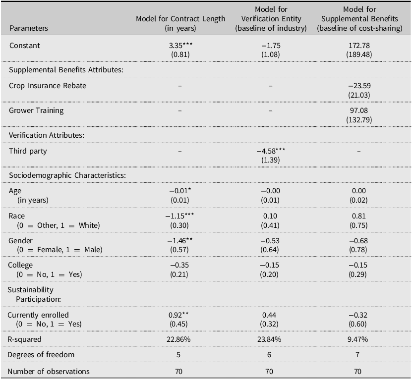
Note: ***indicates significance at 1% level, **indicates significance at 5%, and *indicates significance at 10%.
3.5. Double-bounded contingent valuation results
Regarding the double-bounded contingent valuation questions included in the survey, respondents were first asked if they would be willing to adopt a sustainable practice (i.e, a cover crop, integrated livestock management, row crops, etc.) for $5 per acre. If they responded yes to this initial bid, they were then asked the same question with a bid amount of $2.50 per acre. If they denied the initial bid amount, then the bid amount was increased to $10 per acre. Table 8 presents the estimated WTA amount from the double-bounded contingent valuation portion of the survey. Results show a statistically significant WTA amount of $5.01 per acre, on average, for the adoption of sustainable practices. Johnson et al. (Reference Johnson, Mitchell-McCallister, DeVilleneuve and Berthold2024) reported a WTA value of $26/acre for new cover crop adoption; however, the amounts would be lower for more educated and younger growers or those who have previously utilized cover crops (Bergtold et al., Reference Bergtold, Duffy, Hite and Raper2012; Dunn et al., Reference Dunn, Ulrich-Schad, Prokopy, Myers, Watts and Scanlon2016).
Table 8. Double-bounded contingent valuation results
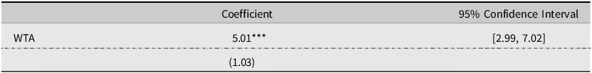
Note: ***indicates significance at 1% level.
Table 9 shows the effects of sociodemographic characteristics on producers’ WTA values for adopting a sustainable practice. Both farming experience and current use of cover crops were statistically significant at the 1% level. Farming experience had a negative effect on WTA with each year increase in experience causing a decrease of $2.08 per acre on WTA. That is, producers with more experience were willing to accept a smaller amount per acre to implement sustainable practices. In contrast, producers who were already employing a sustainable practice in the form of a cover crop would have to be paid $6.16 per acre to adopt and implement additional sustainable practices.
Table 9. Effects of sociodemographic characteristics for double-bounded contingent valuation
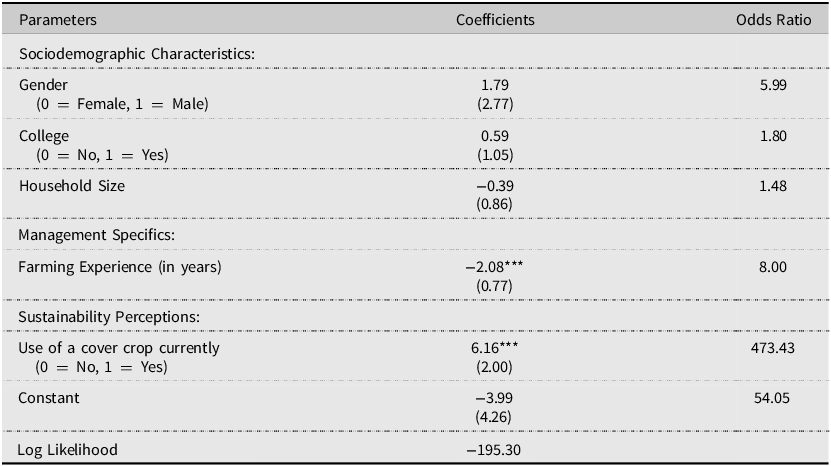
Note: ***indicates significance at 1% level.
4. Discussion and conclusions
The aim of this study was to evaluate growers’ knowledge and perceptions of sustainability programs in agricultural production. After gaining a baseline understanding of how respondents viewed such programs, the goal was to evaluate their preferences for certain contract attributes to determine WTA values for participation in sustainability programs, how various demographic characteristics affected the results, and to determine monetary values producers would require to implement a sustainable practice in their production process.
Results from the mixed logit model and marginal WTA models provide insights on how to meet producer needs for participation in sustainability programs. Overall, the results show producers were willing to pay (i.e., decrease the overall contract price) to increase the length of their contract. Regarding the supplemental benefit for the contract, grower training was the only one to consistently increase the price of the contract instead of yielding a positive value to be interpreted as WTP as cost-sharing did in the per acre contract and crop insurance rebate in both the per acre and per bale contracts. This result also showed that producers may place less importance on the supplemental benefit compared to the other components of a contract. For verification entity, when using the USDA as the baseline both models resulted in a negative value for industry as the verification entity which would increase the overall price of the contract. This shows producers are wary of sharing their production data and would have to be paid more to enroll in a sustainability program that included industry verification. However, third-party verification was positive in the per acre contract (WTP) and negative in the per bale contract (WTA) leading to the conclusion that producers are, overall, indifferent regarding a third-party verification entity.
For both the per acre and per bale contract, a WTP amount was found for length of contract length. This shows producers are willing to decrease the overall amount of a contract in return for an increase in contract length. A crop insurance rebate as the supplemental benefit also yielded a WTP value for both the per acre and per bale contract showing producers were willing to accept a lower contract price if they could have a crop insurance rebate. Also, grower training as the supplemental benefit and industry as the verification entity both yielded WTA values for both models. This shows that producers would rather have no supplemental benefit instead of having grower training and they are wary of sharing their data with industry as both of these attributes increased the overall price of the contract. These results are also supported by a global meta-analysis by Boufous, Hudson, and Carpio (Reference Boufous, Hudson and Carpio2023) who also found agricultural producers will need to be financially incentivized to increase new adoption.
While this study was limited by limited survey responses across one cotton producing region, the results show that producers are willing to enroll in sustainability programs and gives insight into what components make program contracts more appealing to producers. The results for the attributes and their corresponding levels in this study can be used to increase participation rates for producer enrollment in sustainability programs by altering contracts to better reflect producer preferences. Overall, the findings of this study can be used to increase producer willingness to provide their production data, create preliminary contracts for sustainability program enrollment, and to increase overall grower participation.
Data availability
For replication purposes, the data that support the findings of this study are available from the corresponding author, D.M-M., upon reasonable request.
Acknowledgements
None.
Author contribution
Conceptualization, D.M.-M.; Methodology, D.M.-M., and D.H.; Formal Analysis, G.B., T.D.J., and D.M-M.; Data Curation, G.B.; Writing – Original Draft, G.B. and D.M.-M.; Writing – Review and Editing, Q.K. and T.D.J., Supervision, D.M.-M..; Funding Acquisition, D.M.-M.
Funding statement
This project was supported by Cotton Incorporated grant no. 21-444TX and The Cotton Foundation.
Competing interests
Authors declare no competing interest.
AI contributions to research
The study does not involve contributions from artificial intelligence.


 Open access