


The end of the American Civil War brought the end of slavery, but it did not bring the end of the Southern planters. On the contrary, their persistence in power is often thought of as one reason for the South’s slow growth after the war. Their continued political and economic influence led to institutions that favored an agricultural economy with low wages and low education provision (Acemoglu and Robinson Reference Acemoglu and Robinson2006, Reference Acemoglu and Robinson2008a, 2008b). In line with this argument, several papers have found a high wealth persistence in the South after the war (Wiener Reference Wiener1976, Reference Wiener1978; McKenzie Reference McKenzie1993; Dupont and Rosenbloom Reference Dupont and Rosenbloom2018; Ager, Boustan, and Eriksson Reference Ager, Boustan and Eriksson2021). However, relatively little work has documented the persistence of former slave owners in politics, even though the political choices of the Postbellum South clearly reflected their preferences.
This continuity in political power is the focus of our study, which provides systematic evidence for the persistence of slave owners in politics long after the abolition of slavery. We draw on a dataset of Texas state legislators between 1860 and 1900 and link these legislators to their or their paternal ancestors’ census records in 1860. Doing so allows us to calculate the share of each legislature’s members that comes from a slave-owning background. We find that during the American Civil War nearly all Texas legislators were slave owners. Their share dropped substantially during Congressional Reconstruction, but then rebounded and continued on a slow downward trend of only 0.3 percentage points per year till the end of the century. In 1900, still around 50 percent of all state legislators came from a slave-owning background. The share of legislators with more than 20 slaves was even steadier and does not show any downward trend. In 1900, it stood at 11.5 percent, just a bit short of its value in 1861. The high persistence in itself is remarkable. It echoes the high persistence of wealth in the Postbellum South and highlights an important mechanism in how the planter elite kept its de facto power: The former slave owners not only continued to exert control over the productive land, they also remained highly influential in politics.
Does it matter for politics whether legislators come from slave-owning backgrounds? We provide evidence that the likely answer is yes. Former slave owners were more likely to represent the Democratic Party, which at this time constituted the conservative party in the South. Importantly, this holds when controlling for real estate wealth, indicating that the effect is more than a pure wealth effect. Former slave owners were also more likely to serve as committee chairs, suggesting that they were more influential than the average legislator. Drawing on key roll-call votes from three legislatures, we further show that former slave owners voted differently even conditional on party membership: They were more likely to oppose policies that supported blacks’ access to education or the protection of their voting rights and to support the introduction of poll taxes. Consistent with this, we also find that counties that elected more slave owners also displayed worse education outcomes for blacks in the early twentieth century.
Finally, we show that at the county level, the prevalence of slave-owning legislators after the end of Reconstruction is positively correlated with the importance of the cotton economy and with the local persistence of the landed elite after the Civil War. On the other hand, we find Reconstruction-era progress of blacks to be negatively associated with a county’s subsequent propensity to elect former slave owners.
Our paper adds to a large and growing literature on the political economy of the Postbellum South. Canonical accounts include Du Bois (Reference Du Bois1971, writing in 1935), Woodward (Reference Woodward1951), Kousser (Reference Kousser1974), Wright (Reference Wright1986), and Alston and Ferrie (Reference Alston and Ferrie1999). In recent years, especially Acemoglu and Robinson (Reference Acemoglu and Robinson2006, Reference Acemoglu and Robinson2008a, 2008b) have shifted the focus on the planters’ persistence in what they term “de facto political power.” According to this view, continued control over land allowed the antebellum agricultural elite to keep political control of the South. They used this to also keep control over the labor force by blocking land reforms, disenfranchising black voters, and restricting worker mobility. Consistent with this, Ager (Reference Ager2013) shows that counties with a stronger agricultural elite before the war invested less in human capital after the war and had lower labor productivity.
Several studies have analyzed the economic persistence of the planter class. Wiener (Reference Wiener1976, Reference Wiener1978) examined data from five counties in Alabama. He showed that the probability of a rich planter family to remain in a county’s elite was as high after the Civil War as before. McKenzie (Reference McKenzie1993) found similar results for eight counties in Tennessee. Dupont and Rosenbloom (Reference Dupont and Rosenbloom2018) comprehensively analyze the persistence of wealth in both North and South. They find that the rate of persistence of wealthy Southerners was lower than that of their Northern counterparts, but there was still substantial persistence in the South after the Civil War. Ager, Boustan, and Eriksson (Reference Ager, Boustan and Eriksson2021) specifically focus on slave owners and find that the abolition of slavery was a significant negative wealth shock for them, but that their sons and grandsons were able to fully recover these losses. None of these studies looks at the persistence of political power. This is done by Ager (Reference Ager2013) who shows that the majority of delegates in the constitutional conventions of Alabama and Mississippi came from the pre-war elite. However, he focuses on only three points in time— 1865 and 1875 for Alabama, and 1865 and 1890 for Mississippi. To our knowledge, our study is the first that analyzes the persistence of slave owners in regular legislatures and over a long time period.
The advantage of this approach is that it covers the whole evolution of Texas political economy: From the Civil War and its immediate aftermath to Congressional Reconstruction, “Redemption,” the Populist Movement, and finally the early emergence of the “Solid South.” It is remarkable that during all these times the share of former slave owners in the state legislature was usually between 50 and 70 percent and never below 30 percent. Campbell (Reference Campbell1974) and Lowe and Campbell (Reference Lowe and Campbell1975) have analyzed the socioeconomic background of the political leaders in Texas before the Civil War. The latter find that 58 and 68 percent of Texas political leaders held slaves in 1850 and 1860, respectively. While their definition of a political leader is somewhat broader than ours, these values are very similar to what we observe in the 1870s and 1880s, and just a bit above the average in the 1890s. Our results thus indicate that the overrepresentation of (former) slave owners in power hardly changed after the Civil War.
We also show how variables such as the local importance of cotton, local wealth persistence, or the presence of black officeholders correlate with electing slave-owning representatives. In this respect, our study is related to several other recent contributions on the political impact and legacy of slavery. Hall, Huff, and Kuriwaki (Reference Hall, Huff and Kuriwaki2019) show that there was a positive effect of slave ownership on fighting for the Confederacy, while Chacon and Jensen (Reference Chacon and Jensen2020a) find that slave-owning counties were over-represented in the secession conventions in 1861. Logan (Reference Logan2020) uses the within-state distribution of free blacks in 1860 to estimate the causal effect of black policymakers during Reconstruction. He finds that regions with black politicians experienced greater per capita county tax revenue, more land redistribution, and higher black literacy. Relatedly, Chacon and Jensen (Reference Chacon and Jensen2020b) find that the presence of the Union army after the Civil War supported blacks’ political participation. Finally, a recent literature in political science has documented that slavery also mattered in the very long run. Acharya, Blackwell, and Sen (Reference Acharya, Blackwell and Sen2015, Reference Acharya, Blackwell and Sen2016, Reference Acharya, Blackwell and Sen2018) show that whites in regions marked by a greater prevalence of slavery exhibit more conservative political views and higher racial resentment nowadays. For contemporary blacks, a regional heritage of slavery is associated with the lower voting turnout. Much of this persistence can be explained by behavioral path dependence and reinforcing local institutions. Our result that cotton production positively correlates with the persistence of former slave owners in power is in line with these findings.
RECONSTRUCTION AND “REDEMPTION”
The Southern Planter Elite and Reconstruction
The Antebellum South was marked by great wealth inequality, and much of this wealth was in the form of slaves. In 1860, a sample of Southern farmers showed a Gini coefficient for wealth inequality of more than 0.7. Farmers with slaves on average owned 14 times the total wealth of Southern farmers without any slaves (Ransom Reference Ransom1989, p. 63). While it might be too simplistic to conclude from this that the planters were also politically dominant (Wright Reference Wright1978, ch. 2), slave owners were clearly overrepresented among the political leaders of the Antebellum period (Campbell Reference Campbell1974; Lowe and Campbell Reference Lowe and Campbell1975). With the end of the American Civil War, the slave owners lost their slaves, but they kept control over the land. Southern planters were able to fend off attempts at land confiscation or redistribution to the freed slaves, and the plantation units often stayed intact (Wright Reference Wright1986).
Politically, the course of President Andrew Johnson toward the South immediately after the Civil War was lenient. Johnson hoped that loyal Unionists and small farmers would govern the South and lead it back into the Union. However, as put by historian Eric Foner (Reference Foner2006, p. 110) “when the South’s white electorate went to the polls in the fall of 1865 […], it filled the region’s offices with former Confederate generals and public officials.” Frustrated by this, Congress took over. In 1867, it passed the Reconstruction Act over Johnson’s veto. This act divided the South into five military districts and stipulated that the Southern states would not be readmitted before they had accepted universal (male) suffrage (Foner Reference Foner2006, ch. 4 ).
In the following elections, propelled by the vote of the freedmen and by many whites abstaining, the Republicans—the party of Abraham Lincoln and slave emancipation—won all over the South. Biracial governments and legislatures became reality in the South, and over the following years, 2,000 blacks held public offices, despite Klan violence. The resulting state constitutions affirmed racial equality, provided for state school systems, and for other government programs that heretofore had not existed in the South (Foner Reference Foner2006, ch. 5). Public support for Congressional Reconstruction waned, however, in the wake of the financial crisis of 1873, and the federal government loosened its grip on Southern politics. The Democratic Party in the South reconstituted and regained several Southern states, often helped by increasing violence and intimidation of black voters and politicians.Footnote 1 The resulting “Redeemer” governments started to turn the wheel backward. In 1877, as part of the compromise in the close Presidential election, President Hayes ordered federal troops to stop guarding the statehouses in Louisiana and South Carolina. As a consequence, the last Southern state governments fell to the Democrats, and Congressional Reconstruction ended (Foner Reference Foner2006, ch. 7). Eric Foner (Reference Foner2006, p. 198f.) quotes one former slave’s assessment: “The whole South […] had got into the hands of the very men who held us as slaves.”
The Redeemers’ control of the South was not uncontested, though, and black voters did not completely disappear after 1877. However, beginning in the late 1890s, Southern states introduced voting restrictions such as poll taxes or literacy tests. These measures reduced the turnout of black and poor white voters, ensuring a political monopoly of the Democratic Party that would last until the 1960s (Kousser Reference Kousser1974; Foner Reference Foner2006, ch. 7; Besley, Persson, and Sturm Reference Besley, Persson and Sturm2010; Kuziemko and Washington Reference Kuziemko and Washington2018). In addition, the disenfranchisement of black voters, together with the Supreme Court’s Plessy v. Ferguson decision in 1894, also propelled the enactment of Jim Crow laws and the resulting segregation of blacks and whites (Foner Reference Foner2006, ch. 7; Naidu Reference Naidu2012).
The Case of Texas
At first glance, Texas differed somewhat from the other Southern states. It was the westernmost of the 11 states that in 1861 formed the Confederacy, and also the youngest, having been admitted to the United States only in 1845. It was still a very sparsely populated “frontier” state, but at the same time growing fast: Between 1850 and 1860, the population nearly tripled. Economically, it was not as focused on cotton as other Southern states, since for example, ranching was another important driver of its economy. Still, cotton was the state’s most important crop. In 1859, it accounted for more than half the value of the state’s entire agricultural output. Cotton was also closely linked to the institution of slavery. The 1850 census counted roughly 58,000 slaves, and this number rose to more than 182,000 by 1860. Eastern and Northeastern Texas in particular were marked by cotton production and slavery. Along with slavery came a hierarchical social system like in the other Southern states, with a small planter elite at the very top: 72 percent of all slaves in Texas belonged to only 7 percent of the Texan population. Generally, inequality was higher in the older counties in the East than in the younger, recently settled areas in the West (Stephens Reference Stephens2010; Moneyhon Reference Moneyhon2004, ch. 1). Overall, despite the state’s peculiarities, antebellum Texas was also characterized by a cotton-based economy, slavery, and the influence of the slave-owning class.
The political development in Texas after the war was also very similar to the other Southern states, but the transition from Congressional Reconstruction to Redemption occurred even faster. The 11th Legislature was the first one elected after the war, in 1866. Elected during Presidential Reconstruction, it contained so many former Confederate officers that it became known as the “Bloody Eleventh” (Handbook of Texas Online 2013). Its conservative stance is exemplified by the fact that it refused to ratify the 13th and 14th Amendments, which abolished slavery and gave blacks citizenship and equal protection of the laws, respectively. Instead, the 11th Legislature enacted vagrancy and apprenticeship regulations to regulate the labor of freed blacks. Blacks were also precluded from voting and were not allowed to testify in court against whites (Moneyhon Reference Moneyhon2004, ch. 4).
Under Congressional Reconstruction, Governor Throckmorton was removed from office by General Griffin in August 1867. A new constitutional convention was called. This time, blacks were allowed to vote, and voter registration was protected by federal authorities. When the first elections were held under the new constitution, Radical Republicans won a majority in the 12th Legislature. This legislature subsequently ratified the 13th, 14th, and 15th Amendments and created a State Board of Education and a state police force. Texas was readmitted to the United States Congress in March 1870 (Moneyhon Reference Moneyhon2004, chs. 5-7).
The policies of the 12th Legislature led to an increased tax burden, which served as a rallying point for the reorganizing Democrats. They won an overwhelming victory in 1872, with majorities both in the State House and Senate. The 13th Legislature (in session 1873) subsequently abolished the state police and biracial militia companies, reduced the power of the state school superintendent, and redistricted the state so that blacks would find it more difficult to get elected. Many of the laws passed by this legislature reflected the interests of the landowners. For example, by excluding illiterate people from the jury, the legislature increased the power of landowners in civil lawsuits with tenants.
In the 1873 election, which was held without the presence of either the federal army or the state police, black turnout declined across the state. The Democrats won both the governorship and the majority of the legislature. In the following years, through laws and a constitutional convention, the Texas Redeemer Democrats continued with their counterrevolution. They reduced the taxing power of the state government and virtually abolished the state school system, which the Republicans had intended to be a promoter of social change and general education. In addition, the 14th Legislature also passed the “Landlord and Tenant Act,” which greatly increased the rights of landlords over tenants and their crops. State laws also began to separate facilities for black and white citizens, beginning with railroad wagons (Moneyhon Reference Moneyhon2004, chs. 9-12).
Kousser (Reference Kousser1974) cautioned that the victory of the Redeemer Democrats in the 1870s did not mean that they had uncontested control over the South. There was always the danger that a coalition of blacks and poor whites could oust the Democrats. It was only the passage of suffrage restriction laws in the late nineteenth and early twentieth century that completely sealed off this possibility. The same was true in Texas, where the Greenback movement in the late 1870s, the Farmer Alliance in the 1880s, and the Populist Party in the 1890s posed threats for the agricultural elite in power. Using a mixture of concessions to white farmers, violence, and intimidation, and appeals to racial solidarity, the Redeemers were able to fend off these attacks (Moneyhon Reference Moneyhon2004, ch. 12). In 1902 then, after several failed attempts, a poll tax was introduced. This greatly reduced the voter turnout of poor whites and blacks, leaving the Democrats in uncontested power for the next half century (Kousser Reference Kousser1974, pp. 196-209).
DATA
We start from the database “Texas Legislators: Past & Present” (henceforth Texas Database), which is maintained by the Legislative Reference Library of Texas. It contains the names, dates of service, and other information for all members of the Texas State Legislature since 1846. In addition to legislators’ roles in the legislature (dates of services, district and counties represented, party membership, whether they chaired a committee), this database also has biographic details on the legislators such as their birth years and their residence when elected. In addition, for many legislators, it offers links to further biographical resources such as articles about them from the Texas State Historical Association’s Handbook of Texas or on the genealogy webpage Find a Grave™. In the late 1880s and 1890s, this also includes links to biannual publications on the “Personnel of the Texas State Government,” which contained detailed biographical sketches.
Based on the biographical information in this database, we find the census entries of legislators prior to being elected, using the searchable census records provided by ancestry.com. From there, we trace the legislators back to their own or their patrilineal ancestor’s records in the 1860 census.Footnote 2 For all these ancestors, we then collect their 1860 slaveholdings, and their real estate and personal property values. We also record their residence, birth state, birth year, and their occupation, and the number of generations since the 1860 ancestor. Since we focus on legislators serving between 1860 and 1900, for most legislators the difference in generations to 1860 is either 0 or 1: we either find them directly or their parents in 1860. For simplicity, we will refer to the 1860 entry as the “ancestor” of the legislator. Many black legislators were still enslaved in 1860 and hence cannot be matched to an 1860 entry. When we could identify a legislator as black, we coded him as a non-slave owner and a match. There are 43 black legislators in total.
The aim of this paper is to measure whether legislators come from slave-owning families. Because of this, the ancestor will typically be the head of the household in the 1860 census in the patrilineal line from the legislator. In some cases, however, the patrilineal ancestral household contains more members who own property. Within the ancestral household, we, therefore, count the slaveholdings and wealth levels of all the people in this household that are directly in an ancestral line with the legislator. For example, when both father and mother of the legislator own slaves, we add up their slaveholdings. Similarly, if the legislator himself is present in the 1860 census, lives with his parents and does not yet have a family of his own, but some personal property, we also include his property in the wealth measure. However, we do not include the property of siblings (unless the sibling is the household head). In ten cases, the household head is a stepfather. When the legislator (or his ancestor) is present with an older household head, but is clearly already of economically active age and already has a family, we take his values.Footnote 3
In addition to these ancestral data, we also record the legislators’ birth state, and their occupation in the last census prior to being elected. For many legislators elected in the 1890s, this information is missing, since there are no 1890 census records, and many of the legislators were still attending school by the time of the 1880 census.
We could find ancestral data for around 75 percent of our sample of legislators. This match rate is very high compared to studies that have used automated matching.Footnote 4 Battiston (Reference Battiston2018), for example, uses a machine-learning algorithm to match names from ship passenger lists to census records and has a match rate of around 12 percent. Abramitzky, Boustan, and Eriksson (2014) match people across different censuses and obtain a matching rate of 16 percent for natives and 12 percent for immigrants. The reason for our high match rate is the amount of information contained in the Texas Database’s links to biographical information. For many legislators (mostly those serving between 1885 and 1893, and from 1897 on), there are very detailed biographical sketches that often contain parents’ names and complete lists of past residences, which greatly simplifies the task of finding and verifying census records.
Still, the 25 percent unmatched legislators pose the question of whether matched and unmatched legislators are inherently different along certain characteristics. In Online Appendix A, we relate the probability of getting matched to legislator characteristics such as whether the Texas Database contains their full first name or only their initial, how many terms and in which chamber they served, and which party they represented. We find that holding constant the quality of different legislators’ entries in the Texas Database, the match probability does not depend on party affiliations or the role of the legislator in the legislature.
In order to analyze whether former slave owners had different policy preferences, we digitized recorded votes on several key legislative issues. Our first focus is the fight over Reconstruction measures that took place during the 12th and 13th Legislature. We focus on these two legislatures, as they were crucial for the evolution of Reconstruction in Texas. While the Republican-led 12th Legislature (in session 1870/71) attempted to provide the free blacks with access to basic education and voting rights, the 13th Legislature (in session 1873) with its “Redeemer” majority tried to undo most of the changes enacted by the 12th Legislature. Guided by the narrative in Moneyhon (Reference Moneyhon2004), we, therefore, collect recorded votes on the most controversial pieces of legislation in these two legislatures. These include the establishment of a public school system, a militia bill that provided for biracial companies, a voter registration bill, and an act that gave the (Republican) governor the power to fill some vacant public offices. We code these laws as either “progressive” or “conservative” and then classify votes accordingly. The basic idea is that “progressive” votes supported the Reconstruction program of the Republicans, while “conservative” votes aimed at first stopping and later undoing this program. Thus, voting yes on the 1870 education bill that established a system of free school is coded as progressive, while a yes vote on the 1873 bill that repealed the state police act is coded as conservative.
In addition to these Reconstruction-era votes, we also collected recorded votes for two resolutions introduced in the 26th Legislature (in session 1899-1901). Both of these resolutions tried to introduce a poll tax as a prerequisite for voting. As Kousser (Reference Kousser1974, p. 205) notes, both resolutions failed in the 26th Legislature, but both were reintroduced in 1901, and one of them then became the basis for the constitutional amendment introducing a poll tax in Texas. All roll call votes were taken from the respective House and Senate Journals. Details on the laws and the coding of the respective votes can be found in Online Appendix C.
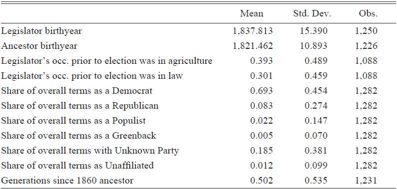
In order to analyze whether the persistence of slave owners in power is related to local socioeconomic characteristics, we calculate a number of county-level characteristics. For a given county, we calculate the share of all legislators that represented this county and that were slave owners. Our interest in this analysis is in the years after the end of Reconstruction. Since the Democrats regained the majority with the 13th Legislature in 1873, we thus calculate the average over Legislatures 13-26, corresponding to the years 1873-1899.Footnote 5 Our explanatory variables for this exercise come from various sources. Based on the 1870 census (Haines et al. 2010), we calculate the county’s cotton intensity, defined as the number of bales produced per acre of improved land. Based on the same source, we also calculate the amount of county tax per capita. Data on black officeholders come from Logan (Reference Logan2019a, 2020). We focus on blacks holding office during Reconstruction and therefore restrict the definition to the years 1867-1872. Counties had between 0 and 5 black officeholders during these times, with the vast majority being in the 0 category. As a result, we code this variable as a simple dummy for having any black officeholder during Reconstruction. Finally, we also create a measure of local wealth persistence. For this, we make use of recent advances in automated linking procedures that allow us to link people across different censuses. Using linking crosswalks from Abramitzky, Boustan, and Rashid (2020) and full-count census data from IPUMS (Ruggles et al. Reference Ruggles, Flood, Goeken, Grover, Meyer, Pacas and Sobek2020), we link white men aged 25-39 in 1860 from the 1860 census to the 1870 one. We then calculate the share of the linked men that were in their county’s top wealth quartile in 1860, still live in the same county in 1870, and are still in the top wealth quartile. We do this separately for total wealth and real estate wealth. This gives us two measures of how persistent the local upper class was. Summary statistics for all variables used in the cross-sectional dataset are shown in Table 1. As can be seen, local persistence in land wealth is larger than in total wealth, which is likely due to the abolition of slavery. In Online Appendix D, we provide a more detailed overview of the construction and sources of these variables.
Table 1 SUMMARY STATISTICS AT THE COUNTY LEVEL

Sources: Authors’ calculation. For data sources, see section “Data” and Online Appendix D.
County borders are taken according to the respective census years.
One problem with this county-level approach is that many electoral districts extend over several counties, creating spatial dependence and a weaker mapping between legislators and county characteristics. A usual remedy would be to aggregate counties to electoral districts and run our analysis at this level, but this is also difficult since electoral districts change frequently. We, therefore, address the spatial dependence in two ways.
Firstly, for this county-level analysis, we focus exclusively on members of the state house and drop all senators, whose districts are considerably larger.Footnote 6 Secondly, in calculating the county-level average of slave-owning legislators, we drop legislators that represented the county when the county was part of a large house district, defined to contain more than 11 counties (the 75th percentile of the distribution of counties per district). In addition, we cluster standard errors at larger geographic units (Bester, Conley, and Hansen Reference Bester, Conley and Hansen2011). To do this, we create an artificial grid of size 100x100 km and then assign counties to this grid depending on their 1890 centroid. By clustering our standard errors at the level of this grid, we allow the errors of all the counties within the same 100x100 km grid cell to be correlated. In the Online Appendix, we show that our results are not sensitive to these choices.Footnote 7
ASSESSING THE PERSISTENCE OF SLAVE OWNERS IN THE TEXAS LEGISLATURE
Table 2 shows cross-sectional summary statistics of the matched legislators. Agriculture and law are the two most common occupations prior to having been elected. Nearly 70 percent of all legislators were working in either of these professions. The majority of legislators were Democrats. Party affiliations here are averaged over a legislator’s total service, in other words, a value of 0.5 for the Democrats means that the given legislator served half of his terms as a Democrat. The vast majority of legislators never changed party affiliation, but there are some exceptions. Only around 8 percent of all legislators’ terms were spent as Republicans, and even fewer with the Populist Party or Greenback Party, which, however, were only active for short time periods. Around 20 percent of legislators’ terms have no party information; this high value is due to the first three legislatures in our sample (elected in 1861, 1863, and 1866, respectively), for which the Texas Database has no party information altogether.Footnote 8 On average, 0.5 generations are between the legislator and the 1860 census ancestor, meaning that in most cases, the match is based on the legislator himself or his parents. This is also in line with the birth years of the legislators and the ancestors, which are separated by around half a generation.
Table 2 SUMMARY STATISTICS AT THE LEGISLATOR LEVEL
Sources: Authors’ calculation. For data sources, see section “Data” and Online Appendix D.
Did legislators come from high socioeconomic backgrounds? The fact that nearly a third of them worked as lawyers, attorneys, or judges indicates so. Further evidence for this comes from Table 3. It shows different wealth measures of legislators’ ancestors and compares them to Texas state averages in 1860 that were obtained from Haines et al. (2010). Nearly 54 percent of all legislators had slave-owning ancestors. Comparing this to the baseline population is not straightforward, since the reference population is not obvious. We, therefore, show two comparisons: In Column (3), we show the ratio of total Texas slaveholders to the number of families. Column (4) instead shows the ratio of slaveholders to the number of white men aged 20 or more. The two shares differ somewhat, but both are substantially below the prevalence of slaveholders among the ancestors of legislators. Thus, the ancestors of the men that became Texas legislators between 1860 and 1900 were considerably more likely to own slaves than the general Texas population in 1860. When looking at certain thresholds, a similar pattern emerges: While 7 percent of all Texan families had ten slaves or more in 1860, 23 percent of all legislator ancestors fell into that category. Moneyhon (Reference Moneyhon2004, p. 11) puts the threshold for belonging to the planter class at owning 20 slaves. Throughout Texas in 1860, less than 3 percent of all families satisfied this criterion, but nearly 10 percent of all legislators had a planter background. In addition, legislators also descended from ancestors that owned more real estate, and more property in general. Texas legislators came from a selected background out of all slaveholders in the state: While the average Texas slaveholder owned 8.3 slaves, the average slave-owning ancestor of a legislator had more than 13. Perhaps most strikingly, while ten slaves was the 75th percentile of slaveholdings in the whole of Texas, 42.5 percent of all slave-owning ancestors had ten or more. Clearly, legislators came from a higher than average socioeconomic background, they were typically from occupations of high standing, and their families in 1860 on average were richer than the average and more likely to own slaves.
Table 3 LEGISLATORS AND AVERAGE WEALTH
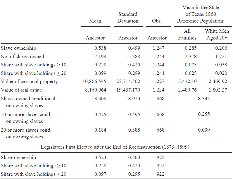
Sources: Authors’ calculation. For data sources, see section “Data” and Online Appendix D.
Figure 1 shows how the share of legislators with slave-owning backgrounds evolved. During the American Civil War, the vast majority of Texas legislators came from a slave-owning family. This share then declined over the 40 years between 1860 and 1900, but remained at around 50 percent by the late 1890s. A clear drop is observed for the 12th Legislature that was elected in 1869, the only such election that took place in Texas during Congressional Reconstruction. The resulting legislature is a clear outlier. The 13th Legislature, elected in 1872 and took office in 1873, brought the Democrats back to power and also increased the share of former slave owners in the legislature back to around 60 percent, a level around which it then stabilized for the following decade. To illustrate how persistent the share of slave owners in the legislature was after the end of Reconstruction, Figure 1 also displays the fitted line of a simple regression of the share of a legislature that has a slave-owning background on time for the post-1873 years. The resulting linear time trend is estimated to be statistically significant and negative, but not very large. It indicates that on average, the share of legislators with a slave-owning background declined by only 0.3 percentage points per year or 3 percentage points by decade.Footnote 9
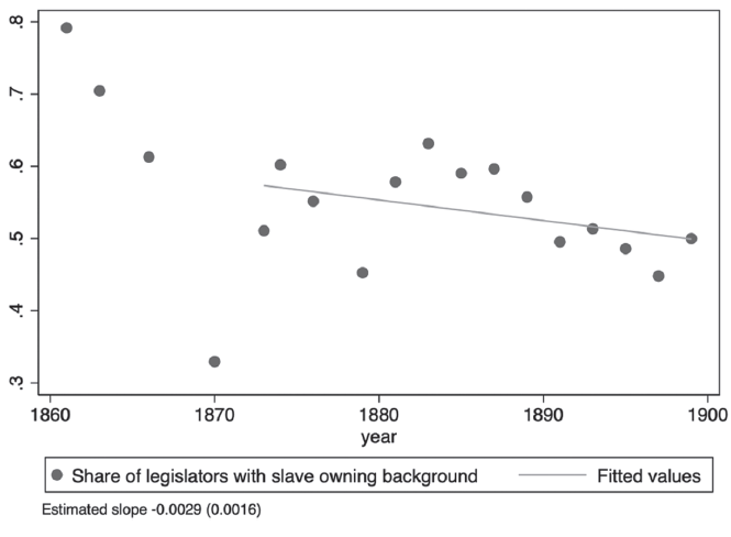
Figure 1 SHARE OF TEXAS LEGISLATORS WITH A SLAVE-OWNING BACKGROUND, 1860–1900
Note: The fitted line shows an estimated linear time trend after the end of Reconstruction in 1873.
Sources: Authors’ calculation. For data sources, see section “Data” and Online Appendix D.
Figure 2 displays the share of legislators with large slave-holding backgrounds (ten or more) over time. This variable fluctuates more and shows even less of a downward trend than the share of legislators with any slave-holding background. There is no drop immediately after the
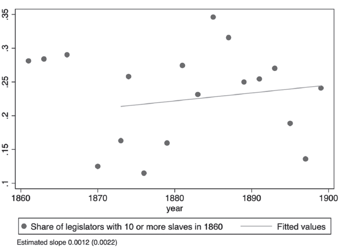
Figure 2 SHARE OF TEXAS LEGISLATORS WITH A LARGE SLAVE-HOLDING BACKGROUND, 1860–1900
Note: The fitted line shows an estimated linear time trend after the end of Reconstruction in 1873.
Sources: Authors’ calculation. For data sources, see section “Data” and Online Appendix D.
Civil War, consistent with the conservative stance of the 11th Legislature, which was elected in 1866 and voted 70-5 against ratification of the 14th Amendment (Moneyhon Reference Moneyhon2004, p. 52). The share then drops in the 1870s, but by 1900 is still at 25 percent. Consistent with this, we estimate the post-Reconstruction linear time trend to be positive, albeit not significantly different from zero.
Finally, Figure 3 looks at the planter elite, those owning 20 slaves or more. Recall that in Texas, less than 3 percent of all families belonged to this bracket. Yet, before the American Civil War, between 10 and 15 percent of all legislators belonged to this group. Again there is a sharp drop for the 12th Legislature in 1870, during Congressional Reconstruction. There is also again a quick rebound after the end of Congressional Reconstruction, and afterward the share fluctuates around its pre-war mean until the 1890s when we see another decrease, followed by an increase by 1900. The linear trend after Reconstruction is estimated to be -0.06 percentage points per year and is not statistically significant.
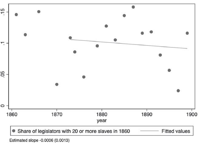
Figure 3 SHARE OF TEXAS LEGISLATORS WITH A PLANTER BACKGROUND, 1860–1900
Note: The fitted line shows an estimated linear time trend after the end of Reconstruction in 1873.
Sources: Authors’ calculation. For data sources, see section “Data” and Online Appendix.
Overall, it becomes apparent that the former slave-owning elite did not only keep its “de facto power.” Slave owners and their ancestors were also powerful in a “de jure” sense, forming a majority in the Texas State Legislature until at least the late 1890s. However, our results also show a noteworthy difference between slave owners and the planter elite: The share of slave owners remained high but declined steadily and by 1899 stood 30 percentage points below its 1861 level. The share of planters, on the other hand, hardly shows any downward trend. Thus, conditional on being former slave owners, the share of former planters increases. This is consistent with the argument brought forward by Oakes (Reference Oakes, Robert and Stephen2015): Due to the changed economic conditions, yeomen farmers and formerly small slaveholders found it increasingly hard to keep their farms. As a consequence, land and power became more concentrated in the hands of former planters.
DOES A LEGISLATOR’S BACKGROUND MATTER?
The fact that former slave owners and their descendants formed a majority in the Texas State Legislature long past the end of slavery is interesting in its own right. It provides further evidence for one important channel through which the old elite managed to keep its de facto power. By holding a majority of the seats in the state legislature, former slave owners shaped the law to reflect their political views. However, this assumes that legislators with slave-owning backgrounds actually had different political views than the average Southern legislator. Perhaps former slave owners were just the most vocal supporters of policies that also would have been supported by state politicians who did not belong to the antebellum elite?
The graphical evidence in Figure 1 seems to suggest a correlation between slave owner prevalence and the policies of a legislature. The 11th and 13th Legislatures, elected in 1866 and 1872, both were marked by policies favoring wealthy whites: abolition of the state police force, restrictions on labor mobility, refusal to ratify the Reconstruction Amendments. They also both had slave owner shares of around 60 percent. The 12th Legislature, on the other hand, with its more progressive policies, also had the lowest share of slave owners during our period of observation.
We therefore next turn to a quantitative analysis of whether legislators with slave-owning backgrounds advocated different policies. We start by examining differences in party membership, a variable that is available for our whole sample. Since it can vary over time, we use our legislator-legislature panel and run regressions of the form
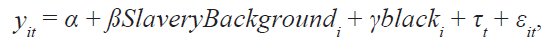 $${y_{it}} = a + \beta SlaveryBackgroun{d_i} + {\rm{ }}\gamma blac{k_i}{\rm{ }} + {\rm{ }}{\tau _t}{\rm{ }} + {\rm{ }}{\varepsilon _{it}},$$
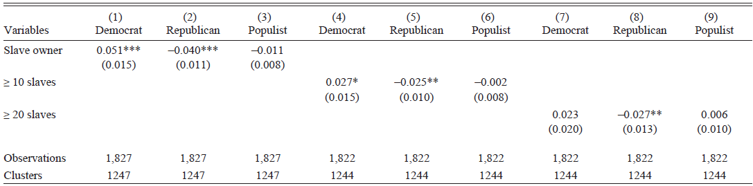
where y is a series of dummy variables for various parties. SlaveryBackground is coded as before via three dummies for having any slaves, 10 slaves or more, or 20 slaves or more. black is a dummy for black legislators and t are legislature fixed effects that control for average changes over time.Footnote 10 Results from these regressions are shown in Table 4. Columns (1)-(3) use a dummy for any slave holdings in 1860 as the main explanatory variable, Columns (4)-(6) use a dummy for slave holdings above 10, and Columns (7)-(9) a dummy for slave holdings above 20.
Table 4 THE RELATIONSHIP BETWEEN LEGISLATOR CHARACTERISTICS AND PARTY CHOICE
Sources: Authors’ calculation. For data sources, see section “Data” and Online Appendix D.
Notes: Regressions control for legislature fixed effects and a dummy for being black. Standard errors, clustered at the legislator level, in parentheses, *** p < 0.01, ** p < 0.05, * p < 0.1
Legislators with slave-owning backgrounds were considerably more likely to be Democrats and less likely to be Republicans. Given the role of the Democratic Party in the Postbellum South, this is not surprising. It confirms the notion that the Democratic Party best represented the interests of the landed elite and indicates that former slave owners on average were more conservative than other legislators. The results regarding large slave owners are usually less precise than for the simple slave-owning dummy, which reflects the lower variation in the large slaveholder dummy variables. The point estimates are usually weaker but remain economically meaningful. We do not find a clear pattern with the Populist Party. This is a bit surprising, given the Populist Party’s policy stance, which according to Goodwyn (Reference Goodwyn1976, p. 297) offered a “nineteenth-century version of ‘black power’” and was partly rooted in “the most radical dream of all - an intersectional, interracial, farmer-labor coalition of the ‘plain people’”(p. 279). However, it has to be kept in mind that this party was only active for four legislatures and is thus a relatively rare occurrence in our dataset.
One issue with the previous results is that in the context of the Postbellum U.S. South, slave ownership might conflate two different aspects of legislator behavior: On the one hand, we use it as a measure of being part of the Antebellum socioeconomic elite. On the other hand, slavery is also a measure of simply being wealthy. This poses the question of whether the differences we observe are due to being former slave owners, or due to just coming from a wealthy background. To analyze this, Table 5 repeats the analysis of Columns (1)-(3) and (7)-(9) of Table 4, but additionally includes the value of real estate owned by the ancestor in 1860.Footnote 11 Real estate wealth is very skewed, and we would ideally use its natural logarithm. This is problematic since many ancestors report no wealth at all. We, therefore, use the inverse hyperbolic sine transformation (Johnson Reference Johnson1949; Burbidge, Magee, and Robb 1988) of real estate wealth, which has become a common practice in such cases. As can be seen, pure real estate wealth does not seem to matter, conditional on being a slave owner. Slave-owning backgrounds, however, are still strongly correlated with party choice.
Table 5 SLAVE OWNINGS AND REAL ESTATE WEALTH
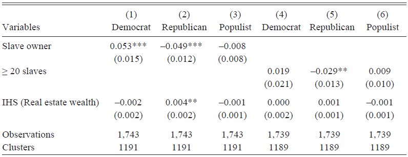
Notes: Regressions control for legislature fixed effects and a dummy for being black. Standard errors, clustered at the legislator level, in parentheses, *** p < 0.01, ** p < 0.05, * p < 0.1
Sources: Authors’ calculation. For data sources, see section “Data” and Online Appendix D.
The evidence so far suggests that slave owners and non-slave owners had different policy preferences. To hone in on this, we turn to analyze key roll-call votes during Reconstruction. In Table 6, we relate a dummy for voting progressively to slave ownership, always controlling for bill fixed effects. Across our three different categories of slave ownership, we find clear evidence that former slave owners voted against progressive policies. Of course, this pattern could simply be due to the fact that slave owners were more likely to be Democrats, and were less likely to be black. In Columns (4)-(6), we therefore additionally control for race and party membership. We find that even compared to white Democrats, former slave owners were still considerably more conservative, especially if they were large slave owners. Even conditional on party membership, slave owning thus seems to have correlated with opposition to Reconstruction and support for “Redemption.”Footnote 12
Given that former slave owners voted more conservatively when it came to black education and political participation, a natural further question is whether we also see worse outcomes for blacks in regions that elected more former slave owners into office. To analyze this, we focus on education as one particularly contentious issue in the Postbellum South. In Table 7, we examine whether counties that elected more former slave owners into power between 1873 and 1899 also provided less education to blacks in the early twentieth century. As outcomes, we use several county-level education measures based on Reference Carruthers and WanamakerCarruthers and Wanamaker (2019): The relative school year length of black students to whites in 1918, the relative annual salary of black teachers to whites in 1925, and the log of total education spending per enrolled student in 1918.Footnote 13 Across all three variables, we see a negative pattern: Counties that continued to elect former slave owners after the end of Reconstruction also had shorter school year lengths for black students relative to whites, paid black teachers less than their white colleagues, and generally spent less on education. These results neatly complement those of Ager (Reference Ager2013), who shows that regions with a stronger Antebellum planter elite had persistently lower levels of labor productivity, literacy, and educational attainment.
Table 6 VOTING BEHAVIOR
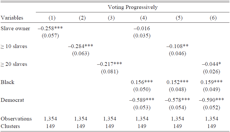
Notes: Voting progressively captures support for the Republicans& Reconstruction measures, see Online Appendix C for details on the recorded votes. Regressions control for bill fixed effects. Standard errors, clustered at the legislator level, in parentheses, *** p < 0.01, ** p < 0.05, * p < 0.1
Sources: Authors’ calculation. For data sources, see section “Data” and Online Appendix D.
Table 7 VOTING FOR SLAVE OWNERS AND EDUCATION SPENDING
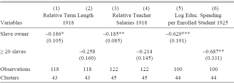
Notes: Robust standard errors, clustered at 100x100 km grid cells, in parentheses. Observations are weighted by the number of matched legislators. *** p < 0.01, ** p < 0.05, * p < 0.1
Sources: Authors’ calculation. For data sources, see section “Data” and Online Appendix D. Relative term length refers to the ratio of the lengths of the school year (measured in days) of black schools relative to white schools in the county. Relative teacher salaries are defined as the ratio of the average annual black teacher salary to the average annual white teacher salary. Spending per enrolled student is defined as the ratio of total school expenditures to the sum of black and white student enrollment.
The evidence so far mostly focuses on slave owners having more conservative preferences regarding the political and economic participation of blacks. Do these differences also extend to the political participation of poor whites? As noted, for example, by Kousser (Reference Kousser1974) and Oakes (Reference Oakes, Robert and Stephen2015), the voting restrictions that many Southern states passed in the late nineteenth and early twentieth century not only virtually disenfranchised black citizens, but also poor white citizens, giving “tiny white minorities in the black belt political power equal to that of overwhelming white majorities elsewhere in the South” (Oakes Reference Oakes, Robert and Stephen2015, p. 156). Were former slave owners and planters more in favor of these measures? To assess this, we collected two roll-call votes from the 26th Legislature in 1899, which aimed at introducing a poll tax. It is already noteworthy that the two legislators that introduced these two resolutions both came from slave-owning families. In Table 8, we analyze whether this is a general pattern, relating whether a legislator voted yes for these resolutions to whether he came from a slave-owning background. As before, Columns (1)-(3) show a simple correlation that only controls for bill fixed effect (which in this case are essentially chamber fixed effects, as each bill only got voted on in one chamber). We find a positive, but insignificant effect for slave owners per se. However, the coefficients for the two wealthier slave owner categories are much larger and statistically different from zero. Former planters, for example, were more than 37 percentage points more likely to support suffrage restriction in 1899. In Columns (4)-(6), we additionally control for party membership in the form of dummies for Democrats and Populists, with Republicans being the omitted reference category.Footnote 14 Not surprisingly, we find that Democrats were considerably more supportive of a poll tax than Populists and Republicans. However, this does not change our conclusions from before: Even conditional on party membership, former planters and large slaveholders were more likely to support suffrage restriction.
Table 8 SUPPORT FOR 1899 POLL TAX BILLS

Notes: All regressions control for bill fixed effects. Robust standard errors in parentheses.
*** p < 0.01, ** p < 0.05, * p < 0.1
Sources: Authors’ calculation. For data sources, see section “Data” and Online Appendix D.
Another way that a legislator’s slave-owning background could have affected the political process is if former slave owners were particularly influential legislators. The influence of legislators is of course hard to measure, but one proxy that we can observe over our whole time period is whether legislators were more likely to chair committees—a common measure for legislative influence (Berry and Fowler Reference Berry and Fowler2018). For this analysis, we create a legislator-legislature panel and run the regression
 $$chai{r_{it}} = a + \beta SlaveryBackgroun{d_i} + {\rm{ }}\gamma blac{k_i}{\rm{ }} + {\rm{ }}{\tau _t}{\rm{ }} + {\rm{ }}{\varepsilon _{it}},$$
where chair is a dummy for whether legislator i chaired one of the committees in legislature t. SlaveryBackground is defined as above. black is a dummy for black legislators and τ are legislature fixed effects that control for average changes over time. Results are shown in Table 9. Columns (1)-(3) use all the legislators between 1860 and 1899, while Columns (4)-(6) focus on the Post-Reconstruction years, beginning with the 13th Legislature. While precision is sometimes low, we find that former slave owners were considerably more likely to chair committees. Former slave owners thus were not only overrepresented in the legislature itself, they were also more influential conditional on being in the legislature.
Table 9 THE RELATIONSHIP BETWEEN SLAVE OWNING AND CHAIRING A COMMITTEE
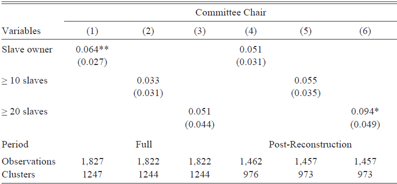
Notes: Regressions control for legislature fixed effects and a dummy for being black. Standard errors, clustered at the legislator level, in parentheses, *** p < 0.01, ** p < 0.05, * p < 0.1
Sources: Authors’ calculation. For data sources, see section “Data” and Online Appendix D.
Overall, our evidence indicates that former slave owners indeed differed from legislators without a slave-owning background. They were more likely to belong to the Democratic Party, even conditional on their wealth levels. During Reconstruction, former slave owners voted more conservatively, even when comparing them to other members of their respective parties, and in the late nineteenth century, they were more fervent supporters of a poll tax that would have disenfranchised a large part of the black and poor white population. Finally, former slave owners were also more likely to be committee chairs and thus had more influence in the legislature than their peers without slave-owning backgrounds.
POTENTIAL DRIVERS OF SLAVE OWNERS’ PERSISTENCE
Which regional characteristics influenced the degree of persistence of former slave owners in power after the end of Reconstruction? To analyze this question, we turn to our cross-sectional dataset that averages the share of slave-owning legislators over time by county. In this analysis, we relate the slave-owning share of all legislators that represented a given county between 1873 and 1899 to several explanatory variables. One potential problem with these county-level results is that Texas counties underwent substantial territorial changes between 1860 and 1890, especially in the Western part of the state. We therefore always show results for our full sample, and for a restricted one that drops all counties whose area between 1860 and 1890 changed by more than 25 percent.
A first potential explanation for the persistence of slave owners in power is the local importance of cotton. We hypothesize that regions with a greater reliance on slave labor and the cotton economy before the war were more likely to continue electing slave owners after the Civil War. This could be due to two different, but related channels: On the one hand, more cotton-intensive counties likely had more slave owners, so that there might have been simply more former slave owners as potential candidates than in counties where the slave economy was less dominant. On the other hand, counties with a greater reliance on cotton might also have had a more politically entrenched planter elite. At the same time, it should be noted that regions with a more intense slave economy also had more black voters after the war and thus potentially more political opposition to former slave owners, at least until voting restriction reduced blacks’ opportunities to vote. To empirically investigate this, we relate the slave-owning share of all legislators that represented a given county during our period of analysis to the county’s cotton production in 1870, measured in bales per acre of improved land. The results of this analysis are shown in Columns (1) and (2) of Table 10. We find a positive and significant correlation between cotton production and the subsequent prevalence of slave owners in power. Increasing the intensity of cotton production by one bale for every 10 acres of improved land is associated with a roughly 6 percentage points increase of the share of subsequently elected legislators that come from a slave-owning background. Areas whose geography is conducive to slave labor thus display a stronger persistence of the former slave-owning elite in power, which is consistent with the findings of Acharya, Blackwell, and Sen (Reference Acharya, Blackwell and Sen2015, Reference Acharya, Blackwell and Sen2016, Reference Acharya, Blackwell and Sen2018) on the long-run effects of slavery.
Table 10 COUNTY-LEVEL CORRELATES OF SLAVE OWING LEGISLATORS
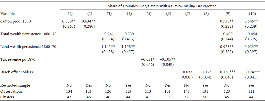
Notes: Robust standard errors, clustered at 100x100 km grid cells, in parentheses. The outcomes code the share of all legislators elected after 1871. The restricted sample removes counties whose are between 1860 and 1890 changed by more than 25 percent. Cotton production in 1870 is measured in bales per acre of improved land. Local wealth persistence is measured as the share of 1860 county residents in the top wealth quartile that still are present in the county’s top wealth quartile in 1870, based either on total or real estate wealth. The presence of black officeholders is measured by a dummy for whether the county had any black officeholders between 1867 and 1871. Observations are weighted by the number of matched legislators. *** p < 0.01, ** p < 0.05, * p < 0.1
Sources: Authors’ calculation. For data sources, see section “Data” and Online Appendix D.
As a second explanation for why slave owners remained in power long after the end of Reconstruction, we consider that their persistence in local political power mirrored their persistence in local economic power. Acemoglu and Robinson (Reference Acemoglu and Robinson2008b) argue that even though slave owners might have lost their slave wealth, they continued to control the land, which in turn kept the basic plantation-based agricultural system intact. Relatedly, Ager, Boustan, and Eriksson (Reference Ager, Boustan and Eriksson2021) show that while the abolition of slavery led to substantial wealth losses for slave owners, this loss was fully recovered by their descendants. We hypothesize that counties with a high degree of wealth persistence also have a high degree of political persistence of the slave-owning class. To examine this, we relate the share of slave owners elected to our two measures of local wealth persistence described earlier. The results of this are presented in Columns (3) and (4) of Table 10. We find a positive correlation of land wealth persistence with slave-owning legislators, which we view as consistent with the argument of Acemoglu and Robinson (Reference Acemoglu and Robinson2008b): In counties where land ownership persisted more, political power persisted more. On the other hand, total wealth persistence has a negative, but insignificant coefficient, which likely reflects the result by Ager, Boustan, and Eriksson (Reference Ager, Boustan and Eriksson2021) that the abolition of slavery was a substantial short-run adverse wealth shock for slave owners.
Finally, we examine the role of Reconstruction-era policies in affecting the persistence of former slave owners in power. Logan (Reference Logan2019b) shows that across the South, there was a violent backlash against black political officeholders in counties where taxes had been particularly increased during Reconstruction. Did this backlash against Reconstruction also manifest itself in electing more former slave owners into office? We use two measures of the local “intensity” of Reconstruction. Columns (5) and (6) of Table 10 show results for tax revenue per capita in 1870, Columns (7) and (8) look at the prevalence of black officeholders between 186772. Interestingly, if anything, we find negative correlations. Tax revenue per capita especially seems to be related in a negative way to the subsequent election of slave owners. The point estimate for black officeholders is also negative, but statistically not significantly different from zero. Taken together, though, these results if anything suggest that former slave owners were less likely to be elected in counties where blacks had made progress during Reconstruction. This could point toward some persistence in these gains. Given the correlational nature of our empirical analysis, we do not want to overinterpret this result. However, a similar persistence in gains in political participation has been found by Ramos-Toro (Reference Ramos-Toro2021), who shows that Southern counties that contained refugee camps during the Civil War displayed lower Democratic vote shares until the late 1880s. In Columns (9) and (10) of Table 10, we introduce all of our measures at the same time.Footnote 15 While the correlation with local wealth persistence becomes weaker, our qualitative conclusions do not change.
Finally, in Table 11, we repeat the analysis from the previous table, but focus on the planter class. Several findings are qualitatively similar: We again find that counties with a high degree of cotton production in 1870 later on elected more planters, whereas the correlation with 1870 tax revenue is negative. The coefficient for land wealth persistence also remains positive and significant. However, there are also some notable differences compared to Table 10. The negative coefficient of total wealth persistence, for example, becomes larger in absolute value and statistically significant. Given that the abolition of slavery affected planters with many slaves more than slave owners with only a few, we find this result plausible and also in line with Ager, Boustan, and Eriksson (Reference Ager, Boustan and Eriksson2021). Another difference compared to Table 10 is that the coefficient for black officeholders in Columns (7) and (8) is now positive. However, as before, this effect is statistically not distinguishable from zero.
Table 11 COUNTY-LEVEL CORRELATES OF PLANTING CLASS LEGISLATORS

Notes: Robust standard errors, clustered at 100x100 km grid cells, in parentheses. The outcomes code the share of all legislators elected after 1871. The restricted sample removes counties whose are between 1860 and 1890 changed by more than 25 percent. Cotton production in 1870 is measured in bales per acre of improved land. Local wealth persistence is measured as the share of 1860 county residents in the top wealth quartile that still are present in the county’s top wealth quartile in 1870, based either on total or real estate wealth. The presence of black officeholders is measured by a dummy for whether the county had any black officeholders between 1867 and 1871. Observations are weighted by the number of matched legislators. *** p < 0.01, ** p < 0.05, * p < 0.1
Sources: Authors’ calculation. For data sources, see section “Data” and Online Appendix D.
CONCLUSION
In this paper, we have examined the persistence of former slave owners in Southern politics after the American Civil War. Using a rich database of Texas State Legislators and census records from ancestry.com, we have linked more than 1,200 legislators to their ancestors and their slaveholdings in 1860. This has allowed us to document the great persistence of the former slave-owning elite in Texas Postbellum lawmaking: Even though only 21 percent of Texas’s 1860 adult white male population owned slaves, slave owners represented more than half of each legislature’s members until the late 1890s. During the brief episode of Congressional Reconstruction, the share of slave owners in the legislature declined substantially, but then rebounded immediately after its end. On average, the share of former slave owners in the legislature declined by only 0.3 percentage points per year after the end of Reconstruction, or 3 percentage points per decade. For planters, the rate of decline is even lower.
We have also shown that legislators with slave-owning backgrounds differ from those without: Over our whole sample period, they are affiliated to the Democratic Party to a greater extent, indicating more conservative political preferences. Consistent with this, we also find that during Reconstruction, former slave owners voted more conservatively in the legislature, even conditional on being Democrats. The continued presence of slave owners in the legislature thus made it harder for the Republicans to implement their Reconstruction measures, and easier for the Redeemer Democrats to undo these very measures later on. At the end of the nineteenth century, former slave owners were more prone to support suffrage restrictions.
Finally, we have documented that the post-Reconstruction persistence of slave owners in power can be partly explained by several local economic factors. The share of former slave owners elected to office is positively correlated with the local intensity of cotton production and with the degree of local wealth persistence in land property. On the other hand, it is negatively correlated with Reconstruction-era tax revenues. Examining the role of other local socioeconomic conditions for the persistence of the old elite should be a fruitful avenue for future research.


 Open access