Recruitment and Service

WWII was the first occasion Australians were conscripted into active wartime service. Compulsory military training existed during 1911–1929, but only volunteers were enlisted into active service in WWI, serving overseas as the Australian Imperial Force (Ville and Siminski Reference Ville and Siminski2011). On the outbreak of war in 1939, a second Australian Imperial Force of volunteers was raised to fight overseas. At the beginning of 1940, compulsory training was resumed. Unmarried men aged 21 were drafted for three months of training and then required to serve for three months (Dennis et al. Reference Dennis, Grey and Morris2008). The conscription coverage gradually broadened over the first two years of the war, eventually being fixed at 18–45 for single men and 18–35 for married men (Ville and Siminski Reference Ville and Siminski2011). Initially, conscripts were only required to serve in Australia, along with New Guinea and adjacent islands. In 1942, as the war in southeast Asia came closer to Australian shores, conscripts could be expected to serve in territories in the “South West Pacific Zone,” which included Indonesia, the Philippines, and Japanese-held islands south of the equator. The Australian Army formed the majority of the defence force, with 728,000 enlisted (Robertson Reference Robertson1981, p. 64), compared with the Royal Australian Air Force (RAAF), with more than 200,000 recruits and the Royal Australian Navy with 37,000 recruits (Beaumont Reference Beaumont2001, pp. 147, 181).

More than half of a million (550,000) Australians went on active service overseas, about 1 in 12 of the population (Beaumont Reference Beaumont1996, p. xx). Their experience of service was highly variable. Only a fraction of recruits were in front line activities that were likely to expose them directly to battle. Some Australians served in units alongside fellow countrymen, whereas others, especially in the RAAF, were part of a broader British Commonwealth force. While many Australians served in New Guinea and nearby Pacific islands, others found themselves in a variety of locations in Europe and the Middle East, which exposed them to quite different forms of engagement. The early campaigns in the Middle East were conducted on flat terrain, with aircraft and artillery bombardments regularly experienced (Gullett Reference Gullett1984). The Pacific saw the majority of combat in heavy jungle, involving close fighting in small groups where the front lines were often inaccessible to larger specialist weapons. Fighting in the Pacific also comprised short and intense engagement, compared with the drawn out battles of attrition in the Middle East (Long Reference Long1973). At least 27,000 Australians died as a result of combat, from wounds, or in prisoner of war camps. A further 23,000 were wounded or injured (Beaumont Reference Beaumont1996, pp. xx, xxv; Long Reference Long1963, p. 634). Probably another 13,000 died in training or in non-combat situations while on service.Footnote ⁷ We do not have data on how many were disabled.

Repatriation

Wartime service impacted upon an individual's workforce opportunities and capabilities. By being removed from the civilian workforce, servicemen missed out on a period of work experience or education and training, which could impact their lifetime earnings and employability. In addition, the physical or psychological damage caused by service could further affect employability. Offsetting these disadvantages, to some degree, were the training, discipline, camaraderie, and teamwork skills that formed part of the military experience (Johnston Reference Johnston1996; Elder and Clipp Reference Elder and Clipp1988; Costa and Kahn Reference Costa and Kahn2003, p. 520).

Repatriation policy in Australia, as elsewhere, recognised that the net effect of wartime service on future employment was probably negative. Compensation policies took several forms. The main compensatory payments of interest, dating back to WWI, were the disability payment (historically called the war pension) along with service pensions paid to veterans on the grounds of age, permanent incapacity to work, or total blindness (Department of Veterans' Affairs (DVA) 2003). Disability payments were based on the level of incapacity. Most countries, including Britain, used deciles working down from 100 percent. For Australia, any incapacity deemed below 10 percent was considered slight enough to warrant no compensation. Britain was slightly more stringent, with anything below 20 percent receiving no compensation (Garton Reference Garton1996, p. 99). Since the Repatriation Act 1920, there is also a special rate of disability pension for those who are totally and permanently incapacitated (TPI), which pays above the normal pension (DVA 2003).

Pension eligibility fell into two categories: those with or without operational service. Operational service included any service outside Australia, and domestic service which incurred danger from hostile forces (DVA 2003). Operational service had no effect on the range or level of compensation, but determined the standard of proof that would be applied. Disability pension claims by veterans with operational service have effectively been assessed under a “reverse-criminal” standard of proof since 1943 (DVA 2003, p. 85). Under this standard of proof, responsibility lay with the Department of Repatriation to prove that a veteran's injury or disability was not a result of military service. A civil standard of proof (balance of probabilities) was applied to claims made by veterans without operational service.

One of the new initiatives for the WWII veterans was the Commonwealth Rehabilitation Training Scheme (CRTS), which was available for all who had served at least six months and were honourably discharged. This was intended to equip and prepare returned servicemen and women with the skills and qualifications to help them re-enter the labor market at the end of the conflict (Garton Reference Garton1996, pp. 81, 98–99). The CRTS provided them with the opportunity to undertake university education or enter technical education or apprenticeships by paying a living allowance and the cost of fees, tools of trade, and books (Lloyd and Rees Reference Lloyd and Rees1994).

In addition to the CRTS and liberal pension offerings, servicemen returned to a period of post-war reconstruction, increased economic activity, and high levels of growth in employment and incomes (Garton Reference Garton1996). Some servicemen may have been incentivized to take the disability pension rather than to work, given the liberal standard of proof. Conversely, the period of increased economic activity and job opportunities may have made servicemen less likely to take the pension.

Further assistance into the workforce was embodied in the employment preference policy. Dating back to WWI, the policy sought to ensure that no ex-servicemen were disadvantaged by employers in seeking to return to the workforce. Anecdotal evidence from disgruntled former servicemen suggests this policy was difficult to monitor and enforce. Even in the public service, where government could exercise a more direct influence, returning servicemen often had to work their way up the ladder in competition with younger employees (Garton Reference Garton1996, pp. 89–91).

Housing Benefits

A severe shortage of housing among discharged servicemen after both world wars motivated a housing benefits policy. Employment disadvantages and absence while on service might impact a veteran's ability to become a home owner. Beginning in 1918, under the Defence Service Homes (DSH) Scheme, veterans who had been on active overseas service were able to access loans to purchase or build their home on terms preferential to the market including low interest rates, no deposit, extended payment terms, and rent-to-purchase provisions. Initially, the government had in mind building houses in blocks to sell to veterans. Within a few years this had failed due to the inexperience of the War Services Homes Commissioner and the urgency of housing demand. In its place, applicants could be funded to build their own home or to buy a new or existing one including refinancing mortgages. This was normally restricted to one loan for one house except when a veteran relocated for work reasons. Such measures continued during and after WWII: the maximum loan amounts were regularly increased and the scope of the policy was extended in 1941 to cover the air force, all nursing services, and spouses (Australian Housing Corporation 1976: part 1, attachments A-G). The United States had a similar scheme as part of the GI Bill (Ingold Reference Ingold1991).

Between 1944–1945 and 1975 there were around 426,000 applications for home loans from among 582,000 qualifying former servicemen, most of whom served in WWII. Of these, approximately 268,000 servicemen had received grants by 1975, a take up rate of 46 percent among eligible veterans (Australian Housing Corporation 1976: part 2, attachments H-O). The Commonwealth-State Housing Agreement (CSHA) was also established in 1945 to address the general housing shortage. It focussed on rental support and allocated 45 percent of its budget to defence force veterans. The revised 1956 CSHA shifted focus to encourage home ownership through low interest rate loans or subsidised purchase prices. But the scheme was dwarfed by the DSH since only 3,402 homes were purchased by ex-servicemen by 1975 through the CSHA (Australian Housing Corporation 1976, p. 61).

First-Stage Data

For the first-stage, we require military participation rates for males by financial year of birth.Footnote ⁹ The numerators of these proportions are estimated using the World War Two Nominal Roll (World War Two Nominal Roll Reference Bound and Turner2002). The denominators are taken from the 1933 and 1947 Australian Censuses.Footnote ¹⁰

The Nominal Roll was created to honour those Australians who served in WWII. It includes data from service records held by the Department of Defence, as well as data from the Commonwealth War Graves Commission for those who died in service. It includes DOB, residency, start and end date of service, date of death, and prisoner of war status. The records are held by the National Archives of Australia.

These counts are subject to measurement error for three reasons. First, the Nominal Roll does not record gender. In personal correspondence, DVA advised that the Nominal Roll includes an estimated 60,000 women overall (or 5.88 percent of the total). Without further information on the age distribution of those women, we assume that this proportion is constant across cohorts, and we deflate the counts accordingly. Second, there are multiple records in the Nominal Roll for some individuals who had a break in service. We have been advised by the data custodians that the extent of such duplication has never been estimated, on the basis that many such duplicates likely contain minor changes in personal details, due either to recording inaccuracy or to enlistees' strategic reasons. Finally, 108,320 records (approximately 10 percent) are missing date of birth (DOB). Those records are excluded. It is difficult to gauge whether the upward bias due to duplicate records is of similar magnitude to the offsetting (10 percent) downward bias due to missing DOB. But the duplication of records would need to exceed 20 percent of the overall count for that count to be biased by more than 10 percent. A further limitation of the Nominal Roll is that it does not flag those who were deployed, and so we cannot attempt to separately identify the effects of deployed and non-deployed service.

The denominator of the participation rates (i.e., counts of men by year of birth) is sourced from published data from the 1933 and 1947 Censuses. The 1933 Census was the last Census prior to WWII and the 1947 Census was the first one after WWII. We regard both as very good proxies for the size of the WWII-era male population by year of birth because migration was low during this era (Phillips, Klapdor, and Simon-Davies Reference Phillips, Klapdor and Simon-Davies2010; Hatton and Withers Reference Hatton, Withers, Ville and Withers2015, p. 352).Footnote ¹¹ When constructing the proportions using 1947 Census counts, we exclude men who died during WWII, since they are obviously excluded from the denominators as well.

Figure 1 shows the resulting estimated WWII participation rates for men born from 1911–1912 to 1939–1940, using the 1933 and 1947 Census counts, respectively, as well as the average of the two.Footnote ¹² Encouragingly, these proportions are not sensitive to the choice of 1933 or 1947 Census counts in the denominators. For the main analysis, we set the military service proportion for each birth year to the average of the two proportions calculated using population counts from the 1933 and 1947 Censuses, respectively.

Notes: The numerators for each birth year are calculated from the World War Two Nominal Roll after adjusting for gender composition. The denominators are taken from the 1933 and 1947 Censuses. For parsimony, 1912 refers to the 1911–1912 financial year birth-cohort, similarly for the other years. The main analysis uses those 17 birth cohorts between the vertical lines. Source: Authors' calculations.

Figure 1 AUSTRALIAN MALE WWII MILITARY PARTICIPATION RATES BY YEAR OF BIRTH

Figure 1 also shows much variation in participation between birth cohorts, with a major drop from 86 percent for the 1924 cohort to just 2 percent in the 1928 cohort. This is due to the conflict coming to an end, and the subsequent reduced need for Australian manpower.

In our main analysis, the first-stage data consist of 17 observations, one for each year of birth between 1917–1918 and 1933–1934. These birth cohorts include approximately 1.02 million Australian men at the end of WWII.Footnote ¹³ This data window was chosen to be centred around 1925–1926, which is the midpoint of the dramatic decline in service participation rates. We conduct extensive sensitivity tests to the bandwidth of this data window.

The upper panel of Table 1 shows descriptive statistics from the first stage database for the main estimation sample. Across the 17 birth cohorts, 46.7 percent of men served in the WWII era. Among those who did serve, 3.6 percent died in service, 2.1 percent were captured as prisoners of war, and the average length of service was 3.25 years.

Table 1 DESCRIPTIVE STATISTICS

∗ The Census collected data on number of rooms in the dwelling in 1966 and 1971, and the number of bedrooms in subsequent years.

Source: The first-stage database was created by the authors drawing on data from the World War Two Nominal Roll and the 1933 and 1947 Australian Censuses. The second-stage data are sourced from the five Australian Censuses of Population and Housing held between 1966 and 1986. In each case, the sample is restricted to men born between July 1917 and June 1934. Post-WWII migrants are excluded from the second-stage data.

Second-Stage Data

The data used in the second-stage regressions are from the five Australian Censuses of Population and Housing held between 1966 and 1986. Using the Australian Bureau of Statistics' customised data service, we obtained a set of tables derived from the full database from each Census, for which 100 percent of the Australian population was in scope. This service is not available for earlier Censuses. Specifically, these were two-way frequency tabulations for a range of outcome variables including labor market status, marital status, housing outcomes, and educational attainment, each by single year of age from each Census.

We used the customised service because these data are not available in published form, nor as microdata. Published two-way frequency tabulations from Census data are generally presented in five- or ten-year age bands, which is not sufficient for our analysis. Microdata sample files are available to researchers to access directly for Censuses held from 1981 onwards, but we preferred to instead draw on the custom tabulations from the full population.

Men who reported arriving in Australia after WWII were excluded from the tabulations. The number of remaining respondent males born between 1917–1918 and 1933–1934 was 958,307 in the 1966 data, declining in each subsequent Census to 808,532 for 1986 due presumably to mortality and emigration. This implies sample attrition rates of between 6 percent (at 1966) and 21 percent (at 1986). Such attrition may be related to military service, though it is not clear how much bias this would contribute to our estimates. We are not aware of any Australian studies that have estimated the link between WWII service and post-service mortality.

The lower panel of Table 1 shows descriptive statistics for each second-stage database, limited to the estimation sample in our main analysis. It shows that 96 percent of men in these cohorts were employed in 1966, when they were 32–48 years old. The corresponding proportions were 93 percent in 1971 and 90 percent in 1976. The proportion unemployed was below 1 percent in 1966 and 1971, and 2.3 percent in 1976, while the remainder were not in the labor force. We do not consider labor market outcomes using 1981 or 1986 Census data, because many of the relevant birth cohorts were aged 60 or over by then. There is a considerable discontinuity in employment rates at age 60 in each Census year, because many people retire at this age. In this context, our strategy of controlling for secular differences between cohorts using polynomial functions of age would not be reliable if the data window were to span those discontinuities.

Table 1 also shows the very low level of university qualifications by this cohort, between 2.9 percent in 1966 and 4.0 percent in 1986. A much higher proportion of men had some form of post-school qualification. In each census, a majority of such qualified men had obtained a trade qualification.Footnote ¹⁴

The proportion of men who were home owners was 70.7 percent in 1966, increasing further with each census up to 76.8 percent in 1986. From 1976 onwards, home-owners with and without a mortgage were separately identifiable. In 1976, slightly more than half of them had a mortgage. By 1986 it was less than a quarter. The proportion living in rental accommodation declined steadily from 21.3 percent in 1966 to 12.2 percent in 1986. In 1966 and 1971, data were collected on the number of rooms in the dwelling. Among men in these cohorts, the average number of reported rooms was 5.6 in 1966 and 5.4 in 1971. Subsequent Censuses instead asked about the number of bedrooms, for which the average response was 2.9 in each year for these cohorts.

Table 1 also shows the progression of marital status between 1966 and 1986. The proportion married was high in all years, but declined from a peak of 83.6 percent in 1971 to 78.8 percent in 1986. The proportion never married also declined from 11.9 percent in 1966 to 8.5 percent in 1986. During this same period, the proportion permanently separated or divorced more than doubled from 3.9 percent to 8.4 percent, and the proportion who were widowers increased by a similar share from 0.8 percent to 4.2 percent.

Our empirical approach relies on the assumption that smooth functions of age adequately control for all non-service factors that vary between cohorts. We scrutinise this assumption for key outcome variables in Figure 2, using 1976 Census data. The upper-left panel shows the proportion of men classified as employed by birth year. This variation is indeed very smooth, at least from the 1917 birth cohort onwards. Indeed, a quadratic function of age explains 99.1 percent of the variation in employment rates between cohorts, after excluding pre-1917 birth cohorts. The discontinuity at age 60 (i.e., between the 1916 and 1917 cohorts) is not surprising, because eligibility for some pensions and annuities commences at age 60. There are similar discontinuities in other Census years. We therefore exclude cohorts older than 60 from any version of the analysis of labor market outcomes. The rationale is that any smooth function of age is not an adequate control for non-service differences between cohorts.

Source: Authors' calculations from 1976 Census of Population and Housing. Males who arrived in Australia after WWII are excluded. The main analysis uses those 17 birth cohorts between the vertical lines.

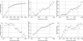
Figure 2 KEY OUTCOME VARIABLES AT 1976, FOR MALES BY FINANCIAL YEAR OF BIRTH

The upper-middle panel of Figure 2 shows a similar scatterplot for attainment of post-school qualification, albeit with a different scale on the vertical axis. This proportion increases steadily between the 1916 and 1926 birth cohorts, falls between the 1926 and 1928 cohorts, then continues its upward trajectory. The corresponding plot for university qualifications follows a similar pattern (upper-right panel), albeit with a less pronounced drop between the 1926 and 1928 cohorts, and with a much smaller proportion throughout.

The lower-left panel of Figure 2 shows the scatterplot for home ownership. Here, there is little variation between cohorts up to the 1925 birth cohort, before dropping steadily for younger birth cohorts. The lower-middle panel shows the unconditional proportion of men that own their home, but have a mortgage. There is much variation in this series across cohorts, varying from around 16 percent for the oldest cohort to 50 percent for the youngest cohort, reflecting life-course differences in mortgage repayment. This variation appears very smooth, but not monotonic. In particular, the series briefly turns downward at the same cohorts where military service rates also fall (Figure 1). A similar pattern is evident in the corresponding plots for the other Census years where this variable is available.

The lower-right panel of Figure 2 shows a corresponding scatterplot, for the proportion of men who were married, which is high for every birth cohort. It is characterised by an upward trend. The proportions for the early-1920s birth cohorts appear somewhat higher than the overall trend.

Labor Market Outcomes

Table 2 shows the estimated effects of military service on labor market outcomes from a series of IV regressions. Since the values of the parameters in the first-stage equation are known without sampling error, there is no first-stage regression output, following Imbens and van der Klaauw (Reference Imbens and van der Klaauw1995), as discussed earlier. Each column shows results for a different Census year.Footnote ¹⁵ Each estimate is derived from models which draw on the 17 birth cohorts centred around 1926 (i.e., 1918–1934), controlling for a quadratic trend in age. The Online Appendix shows extensive sensitivity tests to both the order of the age polynomial and the bandwidth. Unless otherwise specified, the results are not sensitive to these variations in specification.

Table 2 INSTRUMENTAL VARIABLE REGRESSION RESULTS—LABOR MARKET OUTCOMES

Notes: This table shows estimated effects of WWII service on various outcomes, exploiting between-cohort variation in the probability of service through an IV model. The estimation sample consists of the 17 financial-year birth cohorts spanning July 1917 to June 1934. Each regression includes a quadratic function of age. Robust (HC3) standard errors are shown in parentheses. The data sources are described in the notes to Table 1.

^∗ p < 0.10, ^∗∗ p < 0.05, ^∗∗∗ p < 0.01

Source: Authors' calculations.

The proportion of men employed is the dependent variable in Panel A. The estimates for each year are small and quite precise, despite the small number of observations in each regression. There is evidence of a small negative effect on employment in 1966 (–0.4 percentage points), but no evidence of an effect in 1971 or 1976. These results are not generally sensitive to alternate specifications (Online Appendix Table A.1), although the cubic specification does suggest a possible negative effect on employment in 1971 as well.

Panels B and C show results for being not-in-labor-force (NILF) and unemployed, respectively. For 1966, there is a significant positive effect on NILF, which mostly offsets the negative employment effect. The estimated effect on unemployed is small and not statistically significant. There is no evidence that military service affected the chance of NILF or unemployment in 1971 or 1976, mirroring the absence of effects on employment.

This small and temporary effect suggests that most veterans were effectively reintegrated into the civilian labor market, perhaps assisted by government policy to prioritise veterans in public sector recruitment. Moreover, the negative experiences of wartime service should also be set against the positive aspects of training and camaraderie discussed earlier. The results lend only very limited and temporary support to the view that Australian servicemen fared worse in the labor market (Garton Reference Garton1996). That said, employment is a crude measure of labor market outcomes. It would be informative to also study effects on earnings, but such data were not collected in the Census. Furthermore, we cannot rule out more substantial effects on employment in the period between WWII and 1966, for which we do not have data on employment or earnings.

Educational Outcomes

Results for educational outcomes are shown in Table 3, which has the same structure as Table 2, apart from including results for all five census years from 1966 to 1986. Panel A shows that military service had a significant, but relatively modest, effect on post-school qualifications, increasing the rate of attainment by about 3 percentage points at 1971. This effect is equal to about 10 percent of the mean. The CRTS is presumably the mechanism for this effect.

Table 3 INSTRUMENTAL VARIABLE REGRESSION RESULTS—EDUCATIONAL QUALIFICATIONS

Notes: See Table 2 notes.

Source: Authors' calculations.

However, Panel B shows that military service did not have a large effect, if any, on the rate of university qualifications, regardless of which Census year is analysed. This is in stark contrast to the experience of U.S. veterans, for whom the GI Bill greatly increased college education (Bound and Turner Reference Bound and Turner2002).

This is perhaps unsurprising given that 90 percent of CRTS recipients had chosen vocational and technical, rather than university, education (Mackinnon and Proctor Reference Mackinnon, Proctor, Bashford and Macintyre2013, p. 439). Further corroborating evidence for this result is provided by the low prevalence of university qualifications for the 1919–1924 birth cohorts (of whom 90 percent had WWII service). Of these men, only 2.9 percent had obtained a university qualification by 1976. In comparison, 13.0 percent of U.S. men from the same birth cohorts were college graduates by 1970.Footnote ¹⁶

This result conflicts with the conclusions reached by Australian scholars who relate the post-war expansion of university enrolments to the CRTS (Anderson and Eaton Reference Anderson and Eaton1982, p. 10; Groenewegen Reference Groenewegen2009, pp. 57–59). From a very low base, university enrolments expanded considerably after WWII (Booth and Kee Reference Booth and Kee2011, pp. 259–61). But there are other potential explanations for this: pent up demand, regular increases in government funding to the sector including scholarships, and changing popular attitudes and expectations towards tertiary education in the post-war era are all contenders. Our results motivate further research into the reasons for post-war university expansion in Australia.

Housing Outcomes

Results for housing outcomes are shown in Table 4, which follows the structure of the previous two tables. It suggests that the effects on housing were substantial. Panel A shows estimated effects on the probability of being a home owner. It shows evidence that military service increased the probability of home ownership in 1966 substantially (1.8 percentage points). For all later years, the point estimates are around 1 percentage point in each year, although they are not always statistically significant and somewhat sensitive to alternate specifications (Table A.4). Overall, these results suggest that veterans housing benefits did increase the probability of home ownership. The larger estimates for 1966 also suggest that veterans' benefits may have induced some veterans to purchase homes earlier than they would otherwise have done, consistent with Fetter's (Reference Fetter2013) findings for the United States.Footnote ¹⁷

Table 4 INSTRUMENTAL VARIABLE REGRESSION RESULTS—HOUSING OUTCOMES

Notes: See Table 2 notes.

Source: Authors' calculations.

The terms of the DSH Scheme were more favourable than those available from commercial borrowers. Repayment periods of between 32 and 45 years were significantly longer than for commercial loans of around 20 to 30 years. In addition, veterans could effectively borrow 100 percent of the home value—90 percent from the DSH with permission to obtain the remaining 10 percent from another borrower, compared with 70 to 90 percent normally offered by other lenders (Hill Reference Hill, Hirst and Wallace1974, pp. 334–50; Australian Housing Corporation 1976, p. 35). The combination of longer terms and higher loan percentage made it easier for veterans to enter the housing market.

From 1976 onwards, the Census separately identifies home owners with and without mortgages. Panels B and C show results from models that use these as outcome variables. They show that military service had a large negative effect (around 6 or 7 percentage points in each year where we have data) on the probability of being an outright home owner without a mortgage, mirrored by a large positive effect on having a mortgage (around 7 or 8 percentage points). This suggests that the DSH greatly reduced the probability of paying off mortgages. The most likely reason for this is that DSH loans became cheap credit when commercial rates, already above DSH rates since WWII, rose and diverged sharply from the DSH rates from the early 1970s (Figure 3). The role of the DSH in influencing Australian home ownership patterns warrants further investigation.

Sources: Commercial interest rates 1947–1950: Makeham-Kirchner, A (2007) ‘Home loan interest rates and repayments’, Parliament of Australia, http://www.aph.gov.au/About_Parliament/Parliamentary_Departments/Parliamentary_Library/pubs/BN/0708/HomeLoanInterestRates 1950–1959: Reserve Bank of Australia, Australian Economic Statistics 1949–1950 to 1996–1997, Occasional Paper No. 8, No. 3.21b, RBA, Sydney. 1959–1990: Reserve Bank of Australia 2013, Indicator Lending Rates, Cat. No. F5, RBA, Sydney. Defence Service Homes Scheme Although an interest rate of 5 percent per annum was specified in the first War Service Homes Act 1918, the actual rate charged was 3.75 percent from 1946 until the Defence Service Homes Act 1974, when a stepped rate was adopted: 3.75 percent up to $12,000, thereafter 7.25 percent. From March 1980 to November 1988 balances over $15,000, were charged 10 percent. In our Figure, the DSH interest rate between 1974 and 1988 is based on an “average blended rate” calculated by determining the average loan per house. In Defence Service Homes Amendment Act 1988, an interest rate of 6.85 percent was adopted. Malcolm R. Hill, “Housing Finance Institutions” in The Australian Capital Market, edited by Ronald R. Hirst and Robert H. Wallace, p. 349. Melbourne, Australia: Cheshire, 1974. Australian Bureau of Statistics, Year Book Australia, each year 1974–1988, Cat. No. 1301.0, ABS, Canberra.

Figure 3 MORTGAGE INTEREST RATES BY SCHEME AND MONTH

Panel D shows results for the probability of living in a rented dwelling. It shows small negative effects of service, which are statistically significant in 1966 and 1986. These effects are consistent with the positive effects on home ownership in Column 1.Footnote ¹⁸

Panel E of Table 4 shows results for number of (bed)rooms in the residence.Footnote ¹⁹ The number of rooms is a proxy for housing quality. The results suggest that service did not have a large effect on housing quality. If it did have an effect, it seems to have been negative. The point estimates are negative in each year since 1971. However, only for 1981 is it statistically significant at the 5 percent level. The estimate is also largest in 1981, suggesting a reduction in the number of bedrooms by 0.036.

Marital Outcomes

Table 5 shows estimated effects on marital outcomes. The results suggest that effects on marital outcomes are small, but also that they changed over time. The results in Column 1 show little evidence that military service affected marital outcomes in 1966. However, the effect on the probability of being married is positive and highly significant in each of the other Census years (Panel A). While the estimate is rather small in each year, it increases over time, reaching 1.6 percentage points in 1986.

Table 5 INSTRUMENTAL VARIABLE REGRESSION RESULTS—MARITAL STATUS

Notes: See Table 2 notes.

Source: Authors' calculations.

Panels B and C show no significant effects on the probability of being “divorced or permanently separated,” or of being a widower at any of these time points. Panel D shows that the positive effects on being married are largely mirrored by corresponding negative effects on the probability of having never married.

These results suggest that military service induced some men, who otherwise may never have married, to marry for the first time when aged in their 50s. Some caution should be taken with this interpretation, however, given that the point estimates for “never married” in Panel D do not change markedly over the 1966–1986 period. Indeed, the corresponding point estimates for “divorced or permanently separated” in Panel B change slightly more over this period. This suggests that remarriage could also partly explain the positive marriage effect. Regardless, one potential mechanism for the increasing positive effect on being married is veterans' higher pension wealth, which may be advantageous in the marriage market. This is due to earlier eligibility for a retirement pension for the veteran (at age 60, compared to 65 for non-veterans) and for his wife (55 compared to 60), as well as disability compensation payments for many veterans.

In any case, the results do not support the suggestion that WWII service led to family disruption and dissolution, at least later in life (Damousi Reference Damousi2001). Similar results were found by other quasi-experimental studies for Australian veterans of the Vietnam War (Siminski and Ville Reference Siminski and Ville2012), and for U.S. veterans of WWII (Larsen et al. Reference Larsen, McCarthy and Moulton2015) and Vietnam (Conley and Heerwig Reference Conley and Heerwig2013).