WWII prompted one of the largest shifts in female labor supply in U.S. history. Roughly 6.7 million additional women went to work during the war, increasing the female labor force by almost 50 percent in a few short years.Footnote 1 A large share of these new entrants worked in previously male-dominated jobs constructing aircraft, assembling munitions, and staffing a burgeoning federal service. Manufacturing alone accounted for more than three million more female workers between 1940 and March 1944, rising from 21 to 34 percent of total female employment. The arrival of peace, however, ended the wartime boom in female employment almost as abruptly as it began. Female employment declined precipitously in the fall of 1945 and spring of 1946, returning aggregate female labor force participation (FLFP) almost to pre-war levels, as shown in Figure 1.

Figure 1 Civilian Labor Supply and Military Inductions During WWII
A large literature has examined how this impressive but short-lived surge of female workers shaped the post-war course of female employment, particularly for white and married women, who experienced substantial growth in labor force participation rates over the 1940s.Footnote 2 In an important contribution, Claudia Goldin (Reference Goldin1991) used a retrospective survey known as the Palmer Survey to show that women working in 1950 were more likely to have joined the labor force after the war than during it, suggesting limited direct effects of wartime employment by the end of the decade. The limited geographic scope of the Palmer Survey and its focus on married workers, however, left unclear if more comprehensive data might yield different conclusions. A series of recent papers attempts to provide a broader perspective by proxying for geographic variation in the intensity of female wartime work with state-level rates of manpower mobilization for the armed forces, arguing that women entered local labor markets to replace drafted men. This literature finds positive “shocks” to some groups of women’s labor force participation that persisted into the 1950s and beyond, as well as effects on education, intergenerational preference formation, fertility, and other outcomes (Acemoglu, Autor, and Lyle Reference Acemoglu, Autor and Lyle2004; Fernandez, Fogli, and Olivetti Reference Fernandez, Fogli and Olivetti2004; Goldin and Olivetti Reference Goldin2013; Jaworski Reference Jaworski2014; Doepke, Hazan, and Maoz Reference Doepke, Hazan and Maoz2015).
The purpose of this article is to assess the impacts of the WWII boom in female work directly using data on the spatial distribution of more than four million women working in war-related industries in 1943 and 1944 and the placement of women into more than ten million jobs by public employment offices over the same period. This dataset, much of which is new to the literature, allows for a richer characterization of female work during the war, including its geographic concentration and relationship to both industrial and manpower mobilization, as well as its rapid decline when peace arrived. The data also allow me to test directly whether parts of the country exposed to more female wartime work had higher levels of FLFP by 1950 and to contrast these results with similar tests that use manpower mobilization as a proxy.
Three primary results emerge. First, both the data and contemporary documents show that the exigencies of war production appear to have been the primary drivers of the location and intensity of female wartime work. The allocation of military supply contracts across the country is closely related to the quantity of female workers in 1943 and 1944 across a broad set of industries. In many areas, the need for workers in critical war plants drew virtually the entire female workforce into the war effort. For example, in Fort Wayne, Indiana, which was home to a number of converted military vehicle plants, more women were working in war production by the summer of 1944 than were employed in any job in 1940. Manpower mobilization, on the other hand, appears largely unrelated to female wartime employment as measured in these data. These results suggest that labor demand and active recruiting for critical war jobs was a central force behind the wartime female worker boom, rather than draft-induced local labor shortages or shocks to household income as husbands and fathers transitioned to modest military payrolls.
Second, I show that despite large shocks, areas most exposed to the wartime boom in female employment did not see dramatic gains in FLFP by 1950 when compared to less exposed areas. The weak overall effect masks slightly faster growth in durable manufacturing employment and declines in jobs in non-durable goods industries like apparel and textiles, particularly for white women. The same patterns appear across multiple levels of geographic aggregation (states and local labor markets, defined later) and across multiple measures of female wartime employment intensity. The effect on durables, which was a critical driver of the wartime boom, suggests some lasting, direct effects of the war on female employment composition and supports recent parallel work in Price Fishback and Dina Shatnawi (Reference Fishback and Shatnawi2017), who use Pennsylvania data to show that demand for female manufacturing production workers boomed during the war and remained elevated afterwards relative to trends over the 1920s. Declines in non-durables may partly reflect the fact that many war industries drew female workers from existing civilian jobs, leading them to switch industries permanently at the war’s conclusion.
Finally, to understand why the wartime boom did not have a larger impact in 1950, I study the sharp declines in female work in the spring of 1945 and fall of 1946. These declines appear to have been the combined result of layoffs in industries scaling back wartime production, displacement in industries that traditionally favored men or with explicit policies to rehire returning veterans, and large discrepancies in the wages and positions available to laid-off women relative to their wartime work. Detailed records from the U.S. Employment Service (USES) show sharp drops in the female share of job placements exactly when WWII veterans began to rejoin the civilian workforce. The industries that experienced the largest drops in total job placements, such as ordnance, rubber, and aircraft manufacturing, also saw the sharpest declines in female placement shares. Reductions in female labor supply, on the other hand, appear to have been a smaller factor. Women continued to apply for work in large numbers and swelled the unemployment compensation rolls in urban areas like Atlanta, Georgia; Trenton, New Jersey; and Columbus, Ohio. Moreover, changes in female application patterns at USES offices within states in 1946 are unrelated to changes in female placement shares.
These results contribute to substantial literature on the role of WWII in female labor supply changes during the 1940s and after. Although the temporary surge in wartime employment was initially seen as a “watershed” moment for female workers, historians and economists in the 1980s and 1990s argued that the war had little direct impact on female employment in 1950 or after. Goldin’s (Reference Goldin1991) work, already mentioned earlier, was critical to this “revisionist” view. A series of case studies has since provided additional support and context for the view that WWII played a modest role in the growth of female employment over the 1940s. Sherrie A. Kossoudj and Laura J. Dresser (Reference Kossoudj and Dresser1992a, Reference Kossoudj and Dresser1992b), for example, examine employment records for Ford’s Willow Run bomber plant and show that many of the factory’s female workers were laid off and not recalled as the plant converted to peace-time production, despite the fact that jobs requiring similar skills existed at the converted plant. Casey B. Mulligan (Reference Mulligan1998) argues that non-pecuniary incentives were the primary driver of wartime work, perhaps explaining its exceptional and short-lived impact. This article provides an important complement to this literature by directly characterizing the sources of female wartime work’s rise and fall through the expansion and contraction of labor demand for war production, as well as by identifying effects on durables manufacturing employment in 1950.
More recently, a growing literature using manpower mobilization as a proxy for female wartime work has nuanced the revisionist view, finding effects of WWII on female labor supply, education, and other outcomes. The first article to exploit this strategy was Daron Acemoglu, David Autor, and David Lyle (Reference Acemoglu, Autor and Lyle2004), who find that women worked 1.1 more weeks on average in states with 10 percentage points higher mobilization rates. Raquel Fernandez, Alessandra Fogli, and Claudia Olivetti (Reference Fernandez, Fogli and Olivetti2004) show that higher mobilization rates are associated with differences in labor force participation for women likely to have had young children during the war, as well as the subsequent generation’s employment in 1960. Goldin and Olivetti (Reference Goldin2013) find that effects on participation are concentrated among white, married women from the top half of the education distribution, who likely worked in white-collar occupations during the war. Taylor Jaworski (Reference Jaworski2014) uses within-state variation in mobilization across time to argue that exposure to WWII decreased educational attainment among high-school aged women and reduced their later employment and earnings. Matthias Doepke, Moshe Hazan, and Yishay Maoz (Reference Doepke, Hazan and Maoz2015), meanwhile, argue that mobilization-induced labor supply increases intensified labor market competition for women who entered adulthood in the 1950s, leading them to exit the workforce and start families earlier.
The results in this article provide important context for this literature. The draft process, which diverted millions of men from local civilian employment, does not appear to have drawn more women into the workforce to replace them. The weak relationship between female wartime work and mobilization makes it difficult to interpret results that use the latter as a proxy for the former. While mobilization may be associated with female wartime employment in industries not well covered in the data used here or with specific demographic groups’ employment during the war (e.g., white, married women), this is difficult to test without additional information. Interpreting several results in this literature is also complicated by the focus on a labor supply measure that changed definition between the 1940 and 1950 censuses; using alternative, consistent measures suggests that manpower mobilization is correlated with intensive margin increases in labor supply, but not increases in overall participation rates.
The remainder of this article is organized as follows. In the next section, I detail the new and existing data sources analyzed. I then present results on the determinants of spatial variation in female wartime employment. Next, I analyze the relationship between female wartime work, manpower mobilization, and FLFP in 1950. Finally, I analyze the mechanisms behind women’s exit from the labor force after the war.
Data and Sample Construction
I focus here on sources of female wartime employment and job placements data that are new to the literature and refer the reader to previous work for detailed discussions of data that have been used more extensively elsewhere. Across all datasets, an important consideration is the choice of a consistent geographic unit. Because counties are unavailable in public use census data for 1950 and beyond, I use State Economic Areas (SEAs), a grouping of counties within states with similar economic characteristics frequently used in analyses of 1940 and 1950 census data. Because information on wartime female employment is reported for metropolitan areas that straddle state borders, and thus fall into multiple SEAs, I group SEAs that overlap with the same metropolitan area into a new, single, geographic unit.Footnote 3 The results are robust to using alternative geographies, including 1990 Commuting Zones, which were constructed to proxy local labor markets in 1990, but provide good coverage of the metropolitan areas that existed in 1940 as well.
Female Wartime Employment
I use two separate data sources on female employment in the wartime economy. The first consists of reports from the War Manpower Commission’s (WMC) form ES-270, a regular labor force survey of employers in critical war industries and labor markets conducted by local field offices. The survey focused on critical manufacturing and ordnance industries, but also covered employment in government, transport, mining, and other sectors.Footnote 4 ES-270 reports were previously studied by William J. Collins (Reference Collins2001) in the context of fair employment laws, but have not been used to study female workers, to my knowledge.
The WMC produced detailed summaries of these reports for several months between 1943 and 1945, providing point-in-time measures of female employment in metropolitan areas across the United States. The summary reports for July 1944, when total female employment was highest in the data, cover more than 14.3 million employees and 4.6 million women, 3.8 million of whom worked in manufacturing industries, and 438,000 of whom worked in government.Footnote 5 The Bureau of Labor Statistics (BLS) estimated that 5.6 million women were employed in manufacturing in March 1944 (see Table 1), while the U.S. civil service commission lists 1.1 million total female employees in the federal civilian service in 1944 (U.S. Department of Labor 1953, p. 31). This suggests that the ES-270 reports, while not comprehensive, capture a meaningful share of female employment in manufacturing and government, which were the primary drivers of the wartime female employment boom.
Table 1 Shifts in Industrial Composition of Female Employment
Sources and Notes: Totals are reported in thousands. Data for 1940 and 1950 are from U.S. Department of Labor (1953), Table 8, which compiles Current Population Survey Data. Information from March 1944 is taken from U.S. Department of Labor (1944), a special report of the Women’s Bureau analyzing supplemental questions added to the March Current Population Survey. Other includes government positions.
The second source consists of monthly reports on the activities of the USES, a network of public employment offices originally created before WWI and reinstated during the Great Depression to recruit men for President Roosevelt’s Civilian Conservation Corps. During the war, the USES became an important labor market clearinghouse, especially for defense-related industries. By the third quarter of 1944, seven out of ten jobs in manufacturing were filled by the USES, according to the agency (War Manpower Commission 1943–1945, July 1944, p. 40). In 1944 alone, the USES filled 11.4 million jobs, including 3.8 million with women. About 6.8 million of these jobs were in manufacturing industries, with the remainder in retail and wholesale trade, transport, government, and other sectors.
USES activities were detailed in monthly reports published under a variety of names as the department was transferred between agencies over the course of the war.Footnote 6 These reports typically included information on job applications and placements for women, nonwhites, and veterans, often broken down by detailed industry and occupation categories, state, or both. Alongside the job placement data, the reports provided qualitative summaries of the employment situations in a diverse set of industries ranging from airframes to department stores. The reports also contain data from several one-off studies of local labor markets. In what follows, I make use of information from a study of unemployment compensation claimants in Atlanta, Georgia; Columbus, Ohio; and Trenton, New Jersey, in the fall of 1945.
The WMC and USES datasets capture related but distinct aspects of the female employment experience during WWII. While roughly 80 percent of reported employment in the ES-270 data is in manufacturing industries, USES placements data provides broader coverage. During the war, 50 to 60 percent of placements were in manufacturing, with the remainder spread across retail and wholesale trade, services, government, and private households. The two measures remain highly correlated, however: 84 percent of the cross-state variation in total female USES placements is explained by cross-state variation in total WMC female employment in July 1944.
In what follows, I consider total WMC female employment in July 1944 at the state level and in SEAs. I assign WMC employment counts to the combined SEA that contains the metropolitan area listed in the ES-270 reports. The WMC data also report employment in several “unclassified” areas that I am unable to assign to specific SEAs. These areas are excluded from the analysis.Footnote 7 Since the USES data are only available for individual states, I consider total placements from 1943–1945 at that level of aggregation.Footnote 8
Manpower Mobilization
I use several sources of data on manpower mobilization. State-level data come from tables in Selective Service Administration documents, which report the total number of men registered for the draft in each state through 1 September 1945 and the number of men who enlisted or were drafted (Selective Service System 1948). Mobilization intensity is measured as the fraction of registered men who were drafted and enlisted, which given the broad scope of later draft registrations approximates the share of military-aged men who served. The same or similar data are used and discussed in Acemoglu, Autor, and Lyle (Reference Acemoglu, Autor and Lyle2004), Goldin and Olivetti (Reference Goldin2013), and Jaworski (Reference Jaworski2014), all of which provide additional detail on the draft process and mobilization measure.Footnote 9
To measure mobilization at the sub-state level, I use a National Archives database of about nine million individual induction records for the U.S. Army and Army Air Forces (National Archives and Records Administration 1938–1946). The data were created from the Army’s original induction “punch cards” that recorded inductees’ serial number, name, address of residence, rank, height, weight, and other information on paper index cards. In 1994, the National Archives and the Census Bureau converted more than a thousand microfilm rolls of punch card images into a digital format. Because some microfilm roles were unreadable, several blocks of known Army serial numbers are missing. Unfortunately, serial numbers began with two digits that denoted the soldier’s state of origin in clusters of three to nine states. As a result, several states are missing significant shares of total inductions reported in other documents such as Selective Service System (1948).Footnote 10 Online Appendix Figure 1, Panel A maps measured mobilization intensity in the areas where the data provides at least 80 percent coverage of official totals, highlighting the extent of the missing data.
These enlistment records also only cover members of the Army, which comprised the bulk but not totality of U.S. fighting forces. Of the 14.7 million men who served in the Armed Forces by September 1945, 70 percent served in the Army (Selective Service System 1948). The Army’s share was relatively consistent across states, with 41 of 49 continental states and the District of Columbia falling within 5 p.p. of the national average and no clear geographic clustering.Footnote 11 Army enlistments may thus provide a noisy but unbiased measure of total armed forces mobilization.
To obtain a more comprehensive measure of manpower mobilization, I also collect data on total war deaths by county. Army and Army Air Forces data come from War Department documents hosted at the National Archives and known as the “Honor Roles of Dead and Missing” (War Department: The Adjutant Generals’ Office 1946). For each death, the data report either the soldier’s home upon enlistment or, if he gave no address when inducted, the address of his next-of-kin. Data for the Navy, Marine Corps, and Coast Guard were added from similar lists also available at the National Archives (Department of the Navy 1946). If the conditional probability of being killed in action is uncorrelated with other county-level characteristics that influence the outcomes of interest, death rates can provide a noisy but unbiased measure of county-level induction rates. Online Appendix Figure 1, Panel B shows that inductions and war deaths are indeed highly correlated in areas where inductions data provide strong coverage of known totals.
I consider both induction and war death rates at the state and SEA level. In SEA analyses, I normalize by the 1940 male population aged 21 to 54, which roughly captures the population of eligible men. In state-level analyses, I normalize by total draft registrants as in the previous literature studying manpower mobilization. When studying the induction data, I restrict to states where the data captures at least 80 percent of the known totals. The results are not sensitive to similar restrictions (i.e., 70 or 90 percent), but using all inductions data likely introduces bias given the geographic clustering of states with low coverage obvious in Figure 2, Panel A. Similar results are obtained, however, if the data are treated as missing-at-random within states and state fixed-effects are included.

Figure 2 Pre-Trends in Effects of WMC Employment on Labor Force Outcomes
Additional Data
To measure the scale and geography of industrial mobilization for the war, I use measures of county-level spending on WWII military contracts from the Census Bureau’s County Data Book of 1947 (as studied by Fishback and Cullen Reference Fishback and Cullen2013), sourced from Haines and Interuniversity Consortium for Political and Social Research (henceforth Haines and ICPSR Reference Haines2010). This dataset lists total spending on equipment and non-equipment related supplies and facilities between June 1940 and September 1945. Spending is allocated to individual counties if the primary producing plants were located there. I use the sum of spending across all categories and normalize by the 1940 population aged 16 or older.
The core data on female labor market outcomes for each state and local area come from the Integrated Public Use Microdata Series (IPUMS) samples for 1880–1970 (Ruggles, Genadek, Goeken, et al. Reference Ruggles, Genadek and Goeken2017). Whenever possible, I use the 1940 complete count census to construct 1940 measures. I also use ICPSR’s State and County data books to collect additional covariates, such as the share of land devoted to agriculture in each SEA (Haines and ICPSR Reference Haines2010).
Results
Female Wartime Employment
While women worked in war-related industries and were placed into new jobs by the USES in every state across the country, wartime employment was concentrated in select areas in the West Coast, Great Lakes, and the Northeast. The top ten labor markets accounted for more than 40 percent of female WMC employment by the end of 1944, including more than a quarter million in the Chicago area and similar concentrations in Newark-Trenton and Detroit. In Oregon, California, and Washington, meanwhile, the USES placed more than three times as many women into jobs on a per capita basis during the war than in Oklahoma, Nebraska, or Montana.
Of course, areas with substantial WMC employment may have also had more defense-related employment in 1940, making the growth in female employment from 1940 to 1944 more informative than the levels. To construct a growth measure, I take the difference between reported WMC female employment and the number of women working in 1940 in industries reported in the WMC data, which include mining and construction, manufacturing (for both durables and non-durables), transportation, communication and public utilities, and government. The choice of 1940 industries is the same as in Collins’ (Reference Collins2001) study of WMC data and minority employment. Since similarly sized absolute changes in employment may represent relatively small or large shocks depending on each SEA’s size and female employment level, I use the difference in the inverse hyperbolic sine of each year’s female employment as an approximation to the natural logarithm.Footnote 12
The spatial variation in female employment growth is tightly linked to where military contracts increased the need for new workers to rivet, stitch, solder, and otherwise help supply the Allied fighting forces. Online Appendix Figure 2 maps female employment changes (Panel A) and the distribution of wartime military supply contracts per capita (Panel B). Similar spatial concentrations are clearly visible in both maps, such as in the aircraft manufacturing hubs in the Pacific Northwest and the Detroit-area auto hubs. A linear fit suggests that contract spending explains roughly 30 percent of the spatial variation in war-related employment.
In Table 2, I test whether the relationship between WMC employment and military contracts holds conditional on other controls likely to affect female employment during the war. I do so by estimating the following specification: ${\Delta _{1940 - 44}}{\rm{asinh}}\left( {WM{C_s}} \right) = \alpha + {\beta _1}{Z_s} + {\beta _2} {X_s} + {\varepsilon _s},$
where Δ1940–44WMCs is the change in the inverse hyperbolic sine of female WMC employment from 1940 to 1944, Zs is the variable of interest (e.g., wartime contracts per 1940 person aged 16 or older), and Xs is a vector of 1940 characteristics of SEAs. Because the left-hand side is a difference across two time periods only, this specification is equivalent to estimating the effects of a shock (e.g., contracts) on WMC employment in a panel setting with SEA fixed effects included.
Table 2 Female Wartime Employment, Contracts, and Manpower Mobilization

* = Significant at the 5 percent level.
** = Significant at the 1 percent level.
*** = Significant at the 0.1 percent level.
Sources and Notes: The dependent variable is the inverse hyperbolic sine (asinh) of total female WMC employment in July 1944 minus asinh 1940 female employment in industries covered by WMC data (IPUMS 1950 industry codes 200–599 and 900–946), adjusted to have mean zero and a standard deviation of one. War contracts per capita is total spending from 1940–1945 divided by the 1940 population 16 or older. Inductions is total inductions divided by the 1940 male population aged 21–54, and war deaths is total war deaths divided by the same measure. Contracts, inductions, and war deaths measures are also standardized. In columns 3–5, I first use all SEAs, then subset to SEAs where enlistment data cover 80 percent or more of known totals in column 4, then add controls in column 5. Columns 6 and 7 use all SEAs. Regressions are weighted by total SEA population in 1940.
To make coefficient sizes interpretable across specifications, I standardize the outcome and war contracts, inductions, and war deaths measures to have mean zero and a standard deviation of one. Column 1 shows that a one standard deviation increase in war contracts per capita is associated with a 0.50 standard deviation increase in female employment growth. As shown in column 2, the relationship is weakened slightly, but remains large and statistically significant after accounting for 1940 characteristics of SEAs, including the share of employment in manufacturing, white share of population, median schooling for women 25 years or older, and the female labor force participation rate.
These results stand in stark contrast to the relationship between manpower mobilization and female wartime employment. Both manpower mobilization and war deaths exhibit a negative but insignificant unconditional relationship with female WMC employment growth, as shown in column 3 of Table 2. Column 4 shows that this relationship remains similarly weak when only states with at least 80 percent coverage in enlistment data are used. Column 5 shows that the relationship is also small and insignificant after controlling for the same set of 1940 characteristics. Columns 6 and 7 show a similar pattern for war deaths.
To compare these results to the previous literature, I conduct the same exercise at the state level in Table 3, which allows me to use the same mobilization measure as in Acemoglu, Autor, and Lyle (Reference Acemoglu, Autor and Lyle2004) and others. To make comparisons across columns easier, I continue to standardize both the outcomes and explanatory variables to have a mean equal to zero and standard deviation equal to one.Footnote 13 The results paint a similar picture. War contracts are correlated with changes in total female employment, while inductions and war deaths exhibit an either weak or negative relationship.
Table 3 State Level Relationship Between Female Wartime Employment, Contracts, and Manpower Mobilization
* = Significant at the 5 percent level.
** = Significant at the 1 percent level.
*** = Significant at the 0.1 percent level.
Sources and Notes: The dependent variable is the same as in Table 2, except defined at the state level. WMC cities that fall into multiple states are allocated to each state (introducing some double counting), although results are similar if these areas are dropped instead. Only North Dakota has no reported female WMC employment. War contracts per capita is total spending from 1940–1945 divided by the 1940 population 16 or older. Inductions is total inductions divided by male registrants, as studied in the previous literature, and war deaths is total war deaths divided by male registrations. Regressions are weighted by total state population in 1940.
Analyzing state-level information also allows me to make use of USES data on female placements into new jobs, which I do in Table 4. Because no measure of 1940 female job placements is available, however, here I use total placements during the war divided by the 1940 female population aged 16 or older as the outcome of interest. Panel A shows that the state-level relationship between USES placements and contracts and mobilization follows a familiar pattern: Contracts are associated with more placements, both with and without the use of additional controls, while inductions and war deaths are not.
Table 4 State Level Relationship Between Female Uses Placements, Contracts, and Manpower Mobilization
* = Significant at the 5 percent level.
** = Significant at the 1 percent level.
*** = Significant at the 0.1 percent level.
Sources and Notes: The dependent variable in Panel A is total female USES placements 1942–1944 divided by the 1940 female population aged 16 or older. In Panel B it is female placements in clerical and sales occupations divided by 1940 female population aged 16 or older. Explanatory variables are identical to those used in Table 3. Regressions are weighted by total population in 1940. See the Online Data Appendix for additional detail on data construction.
USES placements also provide an opportunity to study female wartime employment in jobs not well covered in WMC data, including positions in white-collar clerical and sales jobs. Goldin and Olivetti (Reference Goldin2013), exploiting mobilization as a proxy for wartime employment, suggest that wartime white collar jobs led to persistent increases in labor force participation for women who were white, married, and more educated. In Panel B, I test the relationship between female placements in clerical and sales occupations and contracts and mobilization. While military contracts are correlated with more white-collar jobs (although the relationship is weaker than in Panel A), inductions and war deaths are not.
Taken together, these results suggest that the geography of rapidly ramping-up wartime production, rather than manpower shortages due to the draft, appears to have driven female employment during the war. There are several reasons why this may be the case. First, female wartime workers were not primarily the wives of soldiers picking up new jobs to supplement meager military pay. In a BLS analysis of special questions added to a CPS survey in the spring of 1944, married women constituted 44 percent of the female workforce, but only 7.7 percent of workers had a husband absent in the armed forces (U.S. Department of Labor 1944). Thus, it does not appear that the bulk of female wartime workers were making up for lost income as the household’s primary earner joined the military.
Second, war industries drove a disproportionate share of the female employment boom. Manufacturing industry jobs climbed from 21 percent of female employment in 1940 to 34 percent by March 1944, with many of the gains coming from ordnance, rubber products, scientific instruments, industrial electrical equipment, and telecommunications equipment essential to the war effort, as shown in Table 1. Areas like Detroit, which was home to a large cluster of defense-related jobs, more than doubled the number of women in their labor force after active recruiting efforts by the USES and local employers (War Manpower Commission 1943–1945, May 1943, p. 12). The scope of labor shortages generated by large-scale war production appears to have dominated any decreases in male labor supply caused by the carefully managed manpower mobilization process. Hence, “the industrial composition of an area largely determines the extent of [female] employment in that area,” as the USES noted in a 1943 report (War Manpower Commission 1943–1945, May 1943, p. 12).
Effects of Wartime Work in 1950
If the WWII employment experience had any immediate effect on female work or industry choice, one would expect areas that experienced more wartime work to have higher levels of FLFP by 1950, either overall or within specific sectors. To test this hypothesis, I employ the difference-in-difference specification from Acemoglu, Autor, and Lyle (Reference Acemoglu, Autor and Lyle2004) using the IPUMS micro samples. The primary estimating equation is: ${Y_{ist}} = {\alpha _s} + {\beta _0}1\left\{ {t = 1950} \right\} + {\beta _1}WM{C_s}1\left\{ {t = 1950} \right\} + {\beta _2}{X_{ist}} + {\beta _3}{X_{ist}}1\left\{ {t = 1950} \right\} + {e_{ist}},$
where Yist is the outcome variable for individual i in SEA s at time t (either 1940 or 1950), αs is a SEA fixed effect, WMCs is the growth in female employment in WMC industry categories from 1940 to 1944, as studied in the previous subsection, and Xist is a set of individual characteristics, such as age, state of birth, and marital status, and SEA-level controls measured as of 1940, such as median education and the white share of the population.Footnote 14 The primary coefficient of interest is β 1, which reflects differential changes in the outcome as a result of variation in WMCs, conditional on all controls. I estimate Specification (2) on the pooled sample of IPUMS 1940 and 1950 census data for all females aged 14 to 64 and not working in farm occupations and industries.
The identifying assumption in Specification (2) is not that war production was randomly assigned across SEAs. Instead, it is parallel trends: β 1 provides an unbiased estimate of the effect of WMC employment intensity on female labor force outcomes in 1950 if, absent differences in WMCs, areas that experienced relatively more wartime employment would have had similar changes in female labor force outcomes from 1940 to 1950 compared to areas that experienced relatively less. Specification (2) also interacts area characteristics such as industrial composition and educational attainment (measured in 1940) with an indicator for 1950 (captured by β 3). This weakens the identifying assumption by instead requiring parallel trends for SEAs with relatively more or less residual variation in WMC employment intensity after controlling for these factors.
What is this source of this residual variation in WMC employment? As noted in the previous subsection, female wartime employment was primarily driven by the location and scale of war production. While much production occurred in existing manufacturing hubs and converted plants, the urgent need for war materials often transformed local labor markets well positioned to supply a critical good in unpredictable ways. For example, in Beaumont, Texas, which the USES described as the “number one boomtown of Texas” in the summer of 1943, the primary pre-war industry was oil and gas refining (War Manpower Commission 1943–1945, Aug. 1943, p. 21). The war, however, transformed Beaumont’s ship building industry. The town had 2,800 workers in six shipyards in 1941 and 29,600 workers in dozens of shipyards in 1943. Women were hired in Beaumont in “ever-increasing” numbers, even in small shipyards that had been “reluctant to utilize women” (War Manpower Commission 1943–1945, August 1943, p. 21). It seems unlikely that production ramped up so dramatically in Beaumont because of characteristics of the local female work force. It is this variation that Specification (2) attempts to isolate.
The main results are presented in Table 5, where the outcome variables of interest are an indicator for whether the individual reported being in the labor force and the total hours worked during the census reference week. Because labor force participation trended differently for all women, white women, and white, married women over this period, I test for effects on these three groups separately in Panels A, B, and C, respectively. As in the previous section, I normalize WMC employment intensity to have a standard deviation of one so that coefficients can be easily interpreted and compared across panels.
Table 5 Impact of Wartime Work on Female Labor Force Participation In 1950
* = Significant at the 5 percent level.
** = Significant at the 1 percent level.
*** = Significant at the 0.1 percent level.
Sources and Notes: Sample includes all female individuals aged 14 to 64 and not working in farming occupations and industries (IPUMS1950 occupation codes 100, 123, 810, 820, 830, 840 and industry codes 105–126). Birth place, age, marital status dummies are indicator variables for place of birth, integer age, and marital status category in the sample. Observations are weighted using the IPUMS-provided census person weights, since no outcomes are sample-line questions. Standard errors are clustered at the SEA level.
The effects in column 1 of Panel A suggest that the unconditional relationship between wartime employment and FLFP growth is very close to zero. Column 2 shows that the results are not affected by the inclusion of individual-level controls, including age, birthplace, and marital status dummies. Column 3, however, shows that after accounting for 1940 characteristics of SEAs, WMC employment appears to have had a modest positive impact on overall FLFP growth. The coefficient reported implies that a one standard deviation increase in WMC employment intensity would generate a 0.3 p.p. increase in FLFP. The results in columns 4–6 show a similar pattern and suggest small positive effects on hours worked after accounting for 1940 controls.
Panel B shows that these results are driven primarily by white women. For this group, effects on both labor force participation and hours worked are positive, although only participation is statistically distinguishable from zero (p < 0.05). The coefficients reported in Panel C for white, married women are similar, although it is more difficult to detect effects due to the loss of precision.
The results in Table 5 are robust to a variety of alternative specifications. Similar effects are obtained, for example, if WMC employment intensity is winsorized by replacing values above the 95th percentile with the 95th percentile, which reduces the influence of several SEAs that experienced exceptionally large employment shocks relative to their 1940 employment base, such as in the naval cluster around Hampton Roads, Virginia. Similar results are also obtained if alternative definitions of WMC employment intensity are used, including normalizing by 1940 female employment or population (instead of using the growth) and excluding all areas that reported no WMC employment. Finally, using 1990 commuting zones instead of SEAs also leads to similar results.
To investigate these small effects further, in Table 6 I estimate Specification (2) with an indicator for participation in various industries and the total hours worked in each industry as the outcome variables. Each cell in the table contains the coefficients and standard error for β 1 from a separate regression. The positive effects reported earlier appear to be driven largely by the durables manufacturing industry, where similar effects are found on both participation and hours worked for all and white women. These effects, however, are partly offset by declines in the non-durables industries. Industry-level effects for white, married women are generally small and insignificant.
Table 6 Sea-Level Impacts by Industry
* = Significant at the 5 percent level.
** = Significant at the 1 percent level.
*** = Significant at the 0.1 percent level.
Sources and Notes: Each cell displays the coefficient and standard error for the relevant labor force outcome in a separate estimation of Specification 2. Hours worked refers to total hours worked in the census references week multiplied by an indicator for participation in the relevant industry. Sample definition is the same as in Table 5. Industries are categorized using the first digit of IPUMS 1950 industry codes. Observations are weighted using the IPUMS-provided census person weights, since no outcomes are sample-line questions. Standard errors are clustered at the SEA level.
The durables manufacturing category includes many industries directly involved with war production, such as aircraft and shipbuilding, electrical machinery, and transport equipment. It seems likely that elevated participation in these industries by 1950 may be the result of wartime work. The non-durables category, meanwhile, includes many relatively female-heavy industries, such as textiles and apparel. War manufacturing industries disproportionately drew female workers from other sectors, as opposed to students and those out of the labor force: 33 percent of the sector’s workers in March 1944 were working in other industries before Pearl Harbor, compared to 24 percent for transport, communication, and public utilities and 14 percent for wholesale and retail trade (U.S. Department of Labor 1944). It thus appears that while wartime employment increased durables manufacturing work for white women, this was partly due to substitution from other industries.
Interpreting the estimates in Tables 5 and 6 as causal requires that the parallel trends assumption discussed earlier holds. While it is not possible to test for parallel trends in counterfactual female labor force outcomes, one can test whether areas exposed to relatively more or less residual WMC employment experienced similar trends before 1940, which I do in Figure 2. Panel A plots the raw data for the share of women in the labor force in SEAs with above and below median female WMC employment intensities residualized on the 1940 SEA characteristics included in all regressions. The two groups trend similarly both before and after the war, supporting the small overall effects reported earlier.
In Panel B, I produce the same figure for the share of women reporting employment in the durables manufacturing industry (analogous figures for the four largest other industries are included in the Online Appendix). The two groups appear to display parallel trends from 1920 to 1940, although high WMC employment areas also experienced faster growth from 1900 to 1920. However, the universe of women asked about their industry changed over this period (see the notes to the figure), making it difficult to interpret the results directly. The gap between the two groups widens considerably in 1950 and 1960, before closing in 1970. The effects detected in 1950, therefore, reflect differential growth after two decades of similar trajectories.
In the previous section, I showed that manpower mobilization is uncorrelated with wartime work in both WMC and USES data. However, it is possible that manpower mobilization drew women into jobs not well covered by these datasets and had independent effects on FLFP growth from 1940 to 1950, as suggested by several previous studies. To test this hypothesis, in Table 7, I re-estimate Specification (2) using inductions and war deaths at the SEA level as the explanatory variable of interest. Unlike WMC employment intensity, however, neither inductions nor war deaths appear to predict changes in female labor force participation from 1940 to 1950, regardless of the demographic group considered. The point estimates for hours worked are positive but generally smaller than those reported for WMC employment and not statistically distinguishable for zero. Encouragingly, results for war deaths and inductions have the same sign and are impacted similarly by controls, supporting the use of the former as a proxy for the latter.
Table 7 Impact of Inductions and War Deaths on Female Labor Supply In 1950
* = Significant at the 5 percent level.
** = Significant at the 1 percent level.
*** = Significant at the 0.1 percent level.
Sources and Notes: Sample and specification are identical to Table 5, except explanatory variables are either inductions or war deaths. Inductions is total inductions divided by the 1940 male population aged 21–54, and war deaths is total war deaths divided by the same measure. Observations are weighted using the IPUMS-provided census person weights, since no outcomes are sample-line questions. Only SEAs with all constituent counties falling in states where at least 80 percent of known total inductions are captured are included in regressions using inductions as an explanatory variable.
To reconcile these results with previous estimates of the effects of mobilization, I replicate the results from Acemoglu, Autor, and Lyle (Reference Acemoglu, Autor and Lyle2004) for all women. The estimating equation is identical to Specification (2), but is estimated across states and uses the state-level measure of mobilization intensity considered in the existing literature as the explanatory variable of interest. Results are reported in Table 8. Column 1 shows that, as in Acemoglu, Autor, and Lyle (Reference Acemoglu, Autor and Lyle2004), there is a positive relationship between increases in total weeks worked. The result is weakened but remains positive and significantly different from zero at conventional confidence levels after the introduction of individual and state-level controls (column 2).
Table 8 Impact of Dependent Variable Choice on Mobilization Estimates
* = Significant at the 5 percent level.
** = Significant at the 1 percent level.
*** = Significant at the 0.1 percent level.
Sources and Notes: Sample is restricted to women ages 14 to 65, not living in Alaska, Hawaii, Nevada, or the District of Columbia, which were omitted from Acemoglu, Autor, and Lyle (2004) either because they were not states at the time or due to large population shifts over the period. Farm employment (IPUMS1950 occupation codes 100, 123, 810, 820, 830, 840 and industry codes 105–126) is excluded. Birth place, age, marital status dummies are indicator variables for each place of birth, age, and marital status category in the sample. As shown in Specification 2, all variables (except state of residence and birth place fixed effects) are interacted with an indicator for year = 1950. In 1950, weeks worked last year was asked only to sample line respondents, so 1950 observations are weighted using sample line weights. 1940 observations are weighted using standard IPUMS-provided census person weights. Standard errors are clustered at the state-year level.
Columns 3 and 4, however, show that these results do not hold for an indicator for positive weeks worked in the last year or labor force participation during the census reference week (columns 5–6). One possible explanation for this difference is the changing definitions of the weeks worked variable between 1940 and 1950. In 1940, census enumerators asked respondents to report the number of full-time equivalent weeks worked in the reference year. A full-time equivalent week was defined as the “number of hours locally regarded as a full-time week for the given occupation” or 40 hours if the respondent was unsure. In 1950, however, enumerators counted a week in which any work was done as a whole week. This change mechanically inflates intensive labor supply measures for part-time workers. A woman working every Monday and Tuesday only, for example, would have reported roughly 10 weeks worked in 1940. This same woman would have reported 52 weeks worked in 1950. It appears that the prevalence of part-time work is also correlated with mobilization in 1940, as shown in Online Appendix Figure 3, which plots mobilization against median weeks worked in 1940.

Figure 3 Uses Placement Patterns
If mobilization is correlated with purely intensive margin increases, however, we should expect similar results using hours worked during the census reference week, which was measured consistently between 1940 and 1950. The estimates in columns 7 and 8 suggest that mobilization is correlated with intensive margin increases in hours. The estimate implies that a one standard deviation increase in mobilization rate (3.5 p.p.) would increase average hours worked by 0.37, or 4 percent of the mean. This estimate suggests some real response to mobilization along the intensive margin, although attributing this effect to wartime female employment is complicated by the weak relationship between the two, as discussed earlier.
Why Did Women Stop Working?
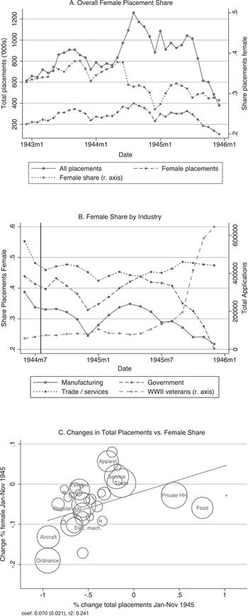
Given the scale of the WWII boom, the modest effects of wartime work on female labor force participation in 1950 might be surprising. Detailed records from the USES can help explain this result. These data reveal that just as industrial mobilization quickly drew women into the workforce, demobilization and the re-integration of veterans into civilian industries appear to have displaced them. Figure 3 Panel A shows that the aggregate female share of USES job placements rose from 32.9 percent at the end of 1942 to 37.7 in mid-1944, before declining to 28.4 percent by the end of 1945. The initial declines, however, were driven by increases in non-female placements. Total female placements remained at roughly 1943 levels before dropping precipitously in mid-1945, when WWII veteran applications and placements began to climb.
These placement declines were concentrated in industries where women competed directly with veterans for jobs. Panel B shows that while the female share of placements in trade/services industries was roughly constant from mid-1945 through the start of 1946, manufacturing and government placements became increasingly male-dominated. The timing of the large declines in female placement shares in government and manufacturing jobs coincided with the return of many WWII veterans, who turned to the USES to find work. Many of these veterans had a legal right to their old jobs or received priority for new ones due to formal and informal “veteran’s preference” rules.
Regular USES reports published at the time provide a remarkable narrative window into the extent of female displacement in the wake of VE Day and VJ Day. A 1946 USES report on the airframe industry, for example, notes that employment opportunities were limited “almost entirely to veterans, who receive preference in nearly all plants” (War Manpower Commission 1943–1945, February 1946, p. 13). In 48 large plants with 160,000 total employees, 4,000 veterans were hired in December 1945, despite net employment declines of 2,000 jobs.Footnote 15 A similar report on the rubber tires and tubes industry, which had been roughly 20 percent female since it became critical in mid-1944, noted “women to be displaced...many employers have indicated to the USES that they expect to replace most of the women on the production line with men” (War Manpower Commission 1943–1945, January 1946, p. 15).
Other industries that were large wartime employers of women, such as the ordnance industry, all but disappeared in 1945. Cutbacks in the industry after VE Day and continuing with VJ Day dropped total employment in ordnance plants from 1,360,000 in March 1945 to 250,000 by September. The female employment share, meanwhile, dropped from 33 to 23 percent (War Manpower Commission 1943–1945, October 1945, p. 11). Government employment also declined significantly. Federal civilian employment in February 1946 stood at roughly 2.4 million, more than half a million less than at the time of Japan’s surrender. While total employment shrank, many veterans returned to reclaim their old jobs at the end of 1945. From July 1944 to the start of 1946, 120,000 veterans had returned to federal service jobs under re-employment rights (War Manpower Commission 1943–1945, February 1946, p. 17). The female share of federal jobs, meanwhile, declined from wartime peaks of 38 to 28 percent by year-end 1946 and 22 percent by 1950, slightly above the 1940 figure of 19 percent (U.S. Department of Labor 1953).
Industries that did not cut back on female workers tended to be those that had traditionally employed women in production and those that did not see sizable cutbacks as the war wound down. A USES report from early 1946 noted that the footwear industry was in dire need of women in jobs overseeing conveyers, operating power sewing machines, and as stitchers (War Manpower Commission 1943–1945, July 1946, p. 21). Men, on the other hand, were needed as shoemakers and assemblers. Even in female-heavy industries, however, wartime occupational and employment gains were often reversed. The USES noted that in the hosiery industry, where two-thirds of employees were female, some women hired to knitting and machine-fixing jobs were “bumped” as veterans returned (War Manpower Commission 1943–1945, October 1946, p. 14).
The patterns shown in Figure 3 Panel C are consistent with this narrative evidence. The graph plots the change in female share of placements over 1945 against the proportional change in total placements for 37 detailed industries. The diameter of the circles corresponds to total female placements in January–March 1945, indicating the industry’s relative importance to wartime female employment. The upward sloping regression line indicates that industries with the largest employment cutbacks also saw the sharpest drops in their female share of job placements.
While this evidence suggests that many women were displaced by returning WWII veterans and laid off in declining industries, it is also possible that as the war wound down, many women simply withdrew from these jobs voluntarily. Several pieces of evidence suggest this is not the predominant explanation for the postwar decline in female labor supply.
First, women continued to apply for jobs from the USES in large numbers. The USES received more than 660,000 new applications for work from women in the first quarter of 1946.Footnote 16 By this point, however, USES placements appear to have shifted towards veterans. The USES received 105,942 job applications from veterans in January 1945, which represented 54 percent of the application pool. It placed 77,735 veterans that same month, for 7 percent of the total. In December, the USES received 644,448 new applications from veterans (66 percent of the total) and placed 116,793 (31 percent of the total). Despite the fact that total placements declined by 65 percent over this same period, veteran placement shares increased roughly four times as much as veterans’ application shares.
Consistent with veterans receiving priority in USES placements, differences in female application patterns across states do not explain differences in female placement shares, as shown in Figure 4 Panel A. Each point on this graph is a state-month combination in January-March 1946. While states with a higher female application share also had a higher female placement share on average, the coefficient on the regression line plotted is 0.549 (se: 0.141), which implies that doubling the female application share would only lead to a 50 percent higher female placement share. Figure 4 Panel B shows that changes in female application patterns are also not associated with changes in female placements within states. Each point in this figure plots the January to March 1946 change in female application share against the January to March change in female placement share for each state. The flat regression line indicates that female application changes are not correlated with shifts in female placements within states.Footnote 17 The USES explained the drops in female placements at the time by noting that “women job seekers have become more sharply limited to the types of jobs which they had held before the war” (War Manpower Commission 1943–1945, January 1946, p. 5).
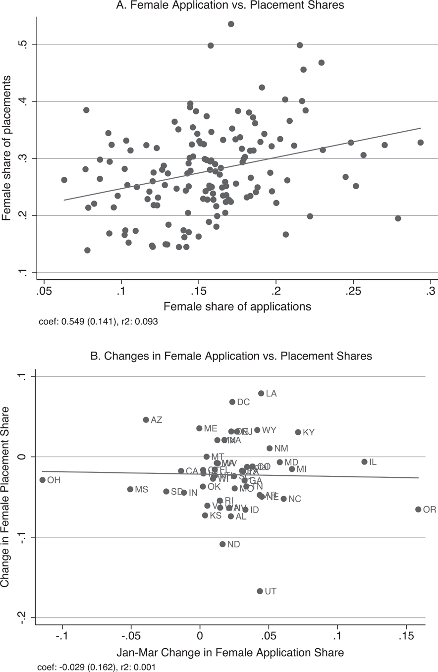
Figure 4 Female Uses Job Applications and Placements
A second piece of evidence comes from a special USES and Bureau of Employment Security study of unemployment compensation (UC) claimants in three cities in the fall of 1945. In Atlanta, Georgia; Trenton, New Jersey; and Columbus, Ohio, in October 1945 women comprised 60, 69, and 77 percent of UC claimants, respectively. The proportion of women is striking given that at their wartime peak in 1945 women comprised roughly 35 percent of the civilian labor force. Being eligible for UC required that these women did not quit voluntarily and were actively looking for work while claiming. Few employers were looking for them, however: 60 to 81 percent of jobs posted in USES offices in these cities specified “men only,” leaving two and half times as many female UC claimants as jobs open for women.
The compensation offered in available jobs at USES offices represented steep wage cuts relative to UC claimants’ previous earnings, especially for women. Matching claimants with available jobs implied a 34 to 49 percent wage cut for men and 49 to 53 percent cut for women. Less than 1 percent of women in Atlanta could have been offered a job paying 90 cents an hour, while 68 percent had previously earned as much. In Columbus, 1 percent of jobs for women were offering wages of 80 cents an hour, while 77 percent of claimants had previously earned as much.
The distribution of UC claimants’ previous and usual occupations relative to the mix in available jobs is also telling. The modal unemployed woman in these three cities left the home to work in a semi-skilled job during the war, but primarily faced low-paying white-collar job opportunities at its conclusion. Roughly 38–50 percent of female UC claimants listed their usual occupation as “housewife” in the three cities. 70 to 75 percent had worked in skilled or semi-skilled occupations in their last job. 50 to 60 percent of available jobs, however, were categorized as professional and managerial, clerical and sales, and service occupations.
According to USES reports, the same pattern repeated itself across other labor markets both during and after the war. After an ordnance plant in St. Louis cut back employment in 1943, for example, the USES noted that “skills developed in ordnance are not generally transferable to other industries, and many of the dismissed women found new employment only by taking pay cuts. In many instances women went from rates of 85 to 90 cents per hour down to 45 to 50 cents” (War Manpower Commission 1943–1945, June 1944, p. 12). Taken together, the USES evidence suggests that the immediate post-war labor market was not favorable to women transitioning successfully from wartime to peacetime employment, especially in jobs that offered comparable compensation to their wartime work.
Conclusion
WWII prompted one of the largest re-organizations of the civilian labor force in U.S. history. As the economy converted to wartime production, women became a central component of the war effort in ammunition plants, shipyards and government offices across the country. But as the war concluded, women left the workforce almost as quickly as they had entered, returning female labor force participation close to pre-war levels.
In this article, I used newly digitized data on the geographic distribution of employment in war-related industries and the activities of public employment offices to argue that despite the size of this experiment in female employment, its impacts on 1950 female labor supply were small. While there are positive effects on white women’s employment in durables manufacturing, these effects are small and partially offset by declines in non-durables jobs. Other recent results arguing that areas that experienced higher rates of manpower mobilization saw larger increases in female labor force participation from 1940 to 1950 are difficult to interpret given mobilization’s weak relationship with female wartime employment. Changing definitions of census variables between 1940 and 1950 also make it difficult to interpret estimates relying on annual weeks worked measures of labor supply. Taken together, the results suggest WWII played a limited direct role in the future course of American women’s employment rates.
Data from the activities of public employment offices, as well as narrative evidence on labor markets and industries at the war’s conclusion, can help make sense of this finding. Women’s exit from the labor force in 1945 and 1946 was the result of mass layoffs in war-related industries, displacement by returning veterans, and poor job opportunities relative to wartime work. Although women’s wartime employment experience was exceptional in its breadth, rewards, and novelty, this short-lived exception to prevailing norms was only made possible by the extreme circumstances of war and was abruptly ended by the arrival of peace.