


1. Introduction
Syringomyelia is a condition characterized by the appearance of slender fluid-filled cavities, known as syrinxes, within the spinal cord (Rizk Reference Rizk2023). An illustration showing the typical location of the syrinx is given in figure 1(a). The condition frequently appears in patients with Chiari I malformation (Milhorat et al. Reference Milhorat, Chou, Trinidad, Kula, Mandell, Wolpert and Speer1999; George & Higginbotham Reference George and Higginbotham2011), a structural abnormality in which the lower part of the cerebellum herniates into the spinal canal, obstructing the normal flow of cerebrospinal fluid (CSF), the colourless Newtonian fluid that bathes the central nervous system. Alternative factors, such as arachnoiditis, spinal cord tumours or physical trauma, can also result in the formation of a syrinx (Klekamp et al. Reference Klekamp, Batzdorf, Samii and Bothe1997; Milhorat Reference Milhorat2000).

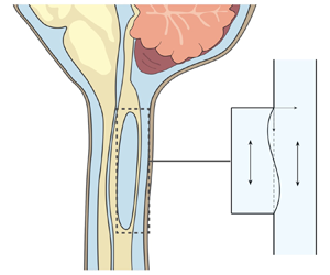
Figure 1. Schematic representation of the problem, including (a) a general view of the central nervous system for a subject having a syringomyelia syrinx at the cervical level, (b) view of the cross-section of the spinal canal at a syrinx-free location, (c) a close view of the cavity with indication of the induced sloshing motion, (d) illustration of the longitudinal flow along the spinal SAS and (e) close view of a spinal cord periarterial space.
The location of the syrinx within the spinal cord depends on the initiating cause. For example, in syringomyelia linked to Chiari I malformation, syrinx cavities typically form in the cervical region of the spine as an expansion of the central canal (canalicular syringomyelia), a CSF-filled space that extends along the spinal cord (see figure 1b,d). In contrast, for syringomyelia associated with spinal cord trauma (post-traumatic syringomyelia), extracanalicular syrinxes generally develop adjacent to the site of the injury (Bertram Reference Bertram2009). The two types of syrinxes are represented in figures 2(a) (canalicular syringomyelia) and 2(b) (extracanalicular syringomyelia), with the former plot depicting a Chiari I malformation (see e.g. Brodbelt & Stoodley (Reference Brodbelt and Stoodley2003), Ahuja et al. (Reference Ahuja, Wilson, Nori, Kotter, Druschel, Curt and Fehlings2017) and Vaquero et al. (Reference Vaquero, Hassan, Fernández, Rodríguez-Boto and Zurita2017) for related clinical images).

Figure 2. Schematic representations of canalicular (a) and extracanalicular (b) syringomyelia, and of the canonical model investigated here (c). The schematic (a) of the canalicular syrinx depicts a Chiari I malformation, while no specific cause is indicated for the extracanalicular case shown in (b).
Despite extensive research, the pathophysiology of the disease remains unclear (Stoodley Reference Stoodley2014). Numerous theories have been advanced over the years (Elliott et al. Reference Elliott, Bertram, Martin and Brodbelt2013). Since the conditions and injuries that precede syringomyelia involve abnormalities in the motion of CSF, it is now generally agreed that CSF flow and its associated pressure variations play an important role in the formation and enlargement of the cavity, as first hypothesized by Gardner & Angel (Reference Gardner and Angel1959).
Magnetic resonance imaging (MRI) techniques have been instrumental in gaining understanding of the CSF flow dynamics. It is now well established that CSF displays an oscillatory motion in the subarachnoid space (SAS) surrounding the spinal cord, as indicated in figure 1(d). The oscillatory velocities, with peak values of the order of a few centimetres per second, are driven by the respiratory and cardiac cycles (Linninger et al. Reference Linninger, Tangen, Hsu and Frim2016; Kelley & Thomas Reference Kelley and Thomas2023), with the former being dominant in the lumbar region (Gutiérrez-Montes et al. Reference Gutiérrez-Montes, Coenen, Vidorreta, Sincomb, Martínez-Bazán, Sánchez and Haughton2022) and the latter being dominant in the cervical region (Yildiz et al. Reference Yildiz, Thyagaraj, Jin, Zhong, Heidari Pahlavian, Martin, Loth, Oshinski and Sabra2017, Reference Yildiz, Grinstead, Hildebrand, Oshinski, Rooney, Lim and Oken2022), where most syrinxes are formed.
Oscillatory motion synchronized with the cardiac cycle has also been observed inside large syrinxes, with associated velocities comparable to those found in the SAS (Brugières et al. Reference Brugières, Idy-Peretti, Iffenecker, Parker, Jolivet, Hurth, Gaston and Bittoun2000; Lichtor, Egofske & Alperin Reference Lichtor, Egofske and Alperin2005). For instance, Vinje et al. (Reference Vinje, Brucker, Rognes, Mardal and Haughton2018) measured peak velocities of 3.6 and 2.0 cm s $^{-1}$ in the SAS and syrinx of a patient with Chiari I malformation, with the values decreasing to 2.7 and 1.5 cm s
 $^{-1}$ after the cavity shrank following surgery. As indicated in the schematic of figure 1(c), the motion in the syrinx displays a sloshing character, with the internal fluid motion inducing cyclic variations of the cavity shape that can be visualized using high-resolution dynamic MRI (Honey, Martin & Heran Reference Honey, Martin and Heran2017). This fluid slosh and its associated pressure fluctuations exert on the surrounding spinal cord tissue a cyclic traction that may contribute to the enlargement of the cavity (Honey et al. Reference Honey, Martin and Heran2017). As revealed by phase-contrast (PC) MRI measurements (Vinje et al. Reference Vinje, Brucker, Rognes, Mardal and Haughton2018), the motion in the syrinx displays multiple oscillations per cardiac cycle, an intriguing feature of the flow resulting from the fluid–structure dynamical interactions taking place.
Central to the pathophysiology of syringomyelia is the physical mechanism that produces the accumulation of fluid within the syrinx (the so-called ‘filling mechanism’; Stoodley Reference Stoodley2014), a key aspect of the problem that remains unclear despite significant research efforts (Williams Reference Williams1980; Klekamp Reference Klekamp2002; Heiss et al. Reference Heiss, Jarvis, Smith, Eskioglu, Gierthmuehlen, Patronas, Butman, Argersinger, Lonser and Oldfield2019; Bhadelia et al. Reference Bhadelia, Chang, Oshinski and Loth2023). Early investigators (Gardner & Angel Reference Gardner and Angel1959; Williams Reference Williams1969) postulated that CSF flows into the syrinx from the fourth ventricle of the brain through the central canal as a result of a dissociation in craniospinal pressure. These initial ideas could not explain, however, the development of the syrinx in patients with an obstructed central canal, that being the case in most adults (Ball & Dayan Reference Ball and Dayan1972; Williams Reference Williams1990; Garcia-Ovejero et al. Reference Garcia-Ovejero, Arevalo-Martin, Paniagua-Torija, Florensa-Vila, Ferrer, Grassner and Molina-Holgado2015).
Alternative theories on the onset of syringomyelia point at a deregulation of the transmedullary flow established between the SAS and the central canal (Oldfield et al. Reference Oldfield, Muraszko, Shawker and Patronas1994; Heiss et al. Reference Heiss1999, Reference Heiss2012; Lloyd et al. Reference Lloyd, Fletcher, Clarke and Bilston2017; Heiss et al. Reference Heiss, Jarvis, Smith, Eskioglu, Gierthmuehlen, Patronas, Butman, Argersinger, Lonser and Oldfield2019). In vivo experiments using injection of fluorescent tracers in sheep, rats and mice have shown that radial inflow and outflow occur predominantly along perivascular spaces surrounding blood vessels (Stoodley, Jones & Brown Reference Stoodley, Jones and Brown1996; Stoodley et al. Reference Stoodley, Brown, Brown and Jones1997; Wei et al. Reference Wei, Zhang, Xue, Shan, Gong, Wang, Tao, Xu, Zhang and Wang2017; Liu et al. Reference Liu, Lam, Sial, Hemley, Bilston and Stoodley2018, Reference Liu, Bilston, Flores Rodriguez, Wright, McMullan, Lloyd, Stoodley and Hemley2022). For instance, as shown by Wei et al. (Reference Wei, Zhang, Xue, Shan, Gong, Wang, Tao, Xu, Zhang and Wang2017), when the tracer is released in the surrounding SAS, inflow occurs mainly along the perivascular space surrounding penetrating arterioles (see figure 1e). This phenomenon has been addressed by Bilston, Stoodley & Fletcher (Reference Bilston, Stoodley and Fletcher2010), who investigated effects of changes in the timing of SAS pressure on perivascular flow into the spinal cord, and by Elliott (Reference Elliott2012), who developed one-dimensional models of transmedullary flow accounting for the presence of perivascular spaces. Transmedullary tracer dispersion is assisted by interstitial flow through the parenchyma (Wei et al. Reference Wei, Zhang, Xue, Shan, Gong, Wang, Tao, Xu, Zhang and Wang2017), at different rates in grey and white matter (Liu et al. Reference Liu, Lam, Sial, Hemley, Bilston and Stoodley2018). The role of the spinal-cord-tissue poroelasticity in the interstitial flow across the spinal cord has been investigated both numerically (Støverud et al. Reference Støverud, Alnæs, Langtangen, Haughton and Mardal2016) and analytically (Cardillo & Camporeale Reference Cardillo and Camporeale2021). An imbalance between the inflow and outflow of CSF, associated with alterations of the transmedullary pressure difference, may lead to accumulation of fluid within the cavity. In this regard, Ball & Dayan (Reference Ball and Dayan1972) suggest that sudden increases in thoracoabdominal pressure could force CSF into the cord, while Oldfield et al. (Reference Oldfield, Muraszko, Shawker and Patronas1994) argue that accentuated pressure waves transmitted by the downward displacement of the cerebellar tonsils during systole play a main role in syrinx formation. A key observation regarding syringomyelia is that the accumulation of fluid is very slow relative to the hydrodynamic time scales (Elliott et al. Reference Elliott, Bertram, Martin and Brodbelt2013), with the consequence that even quantitatively small changes of the existing pressure field, associated for instance with alterations of the normal CSF flow, may have a significant effect when acting over the long time scales characterizing cavity growth.
Numerical simulations and in vitro experiments have been extensively used to investigate different aspects of syringomyelia hydrodynamics (Elliott et al. Reference Elliott, Bertram, Martin and Brodbelt2013). One-dimensional inviscid propagation of large-amplitude pressure waves along elastic channels was studied by Carpenter and co-workers (Berkouk, Carpenter & Lucey Reference Berkouk, Carpenter and Lucey2003; Carpenter, Berkouk & Lucey Reference Carpenter, Berkouk and Lucey2003) to ascertain whether the interactions of a large pressure impulse (e.g. generated by a cough or sneeze) with partial obstructions of the spinal canal could lead to damage of the cord tissue, a hypothesis not supported by subsequent studies (Bertram, Brodbelt & Stoodley Reference Bertram, Brodbelt and Stoodley2005; Bertram Reference Bertram2009; Elliott, Lockerby & Brodbelt Reference Elliott, Lockerby and Brodbelt2009). The sloshing motion induced in the syrinx by a periodic pressure gradient has been investigated numerically (Bertram Reference Bertram2010; Drøsdal et al. Reference Drøsdal, Mardal, Støverud and Haughton2013; Vinje et al. Reference Vinje, Brucker, Rognes, Mardal and Haughton2018) and experimentally (Martin et al. Reference Martin, Labuda, Royston, Oshinski, Iskandar and Loth2010). The studies of Bertram (Reference Bertram2010) and Martin et al. (Reference Martin, Labuda, Royston, Oshinski, Iskandar and Loth2010) considered a spinal cord with a large fluid-filled cavity adjacent to a SAS stenosis. As noted by Bertram (Reference Bertram2010), the cycle-averaged pressure distribution resulting from fluid–structure interaction (FSI) involves a transmural pressure difference that could potentially drive CSF across the spinal SAS into the syrinx, a finding further corroborated in subsequent computations accounting for the permeability of the spinal cord (Heil & Bertram Reference Heil and Bertram2016; Bertram & Heil Reference Bertram and Heil2017).
Like the analyses mentioned in the preceding paragraph, the present paper addresses syringomyelia hydrodynamics, including the sloshing motion induced in the cavity by the oscillating SAS flow and the resulting transmural pressure. Unlike the previous investigations, however, our study is fundamentally analytic in nature, the aim being to clarify the essential FSI dynamics of syringomyelia cavities with use of a simple canonical model problem that affords description of elastic interactions between a confined fluid space and an open canal with oscillatory flow. In some sense, our approach is similar to that followed in investigating oscillations in collapsible tubes (Grotberg & Jensen Reference Grotberg and Jensen2001; Heil & Hazel Reference Heil and Hazel2011), for which the simple Starling resistor (Knowlton & Starling Reference Knowlton and Starling1912) is used as an idealized canonical representation of the flow. Both planar and axisymmetric configurations have been employed (Heil & Hazel Reference Heil and Hazel2011). The former, often used in Navier–Stokes simulations of the flow (Heil & Hazel Reference Heil and Hazel2011), consists of a two-dimensional (2-D) channel in which a finite section of one of the rigid walls is replaced by a deformable wall, represented by a prestressed elastic membrane that separates the channel fluid from a pressure chamber. Wall deformations are induced by the viscous pressure variations in the channel flow, with the wall stiffness dominated by the axial tension of the membrane, leading to complicated FSI dynamical behaviours (Grotberg & Jensen Reference Grotberg and Jensen2001; Heil & Hazel Reference Heil and Hazel2011).
As shown in figure 2(c), the present analysis employs a variant of the 2-D Starling resistor to investigate the two-way-coupled dynamics between the oscillatory flow in the spinal SAS, represented by an infinite channel of constant thickness, and the oscillatory flow in the syrinx, represented by a slender rectangular cavity, with an impermeable elastic membrane subject to longitudinal tension used to model the thin layer of spinal cord tissue separating both spaces. As indicated in figure 2, this 2-D configuration, chosen here to maximize analytic simplification, can be envisioned as an approximate representation of extracanalicular syrinxes, with the rigid wall opposing the membrane representing the internal spinal cord tissue. It is worth mentioning that the use of the 2-D model neglects the hoop stresses induced by the azimuthal stretching of the tube, which can be important, especially for canalicular syrinxes, for which an axisymmetric configuration appears to be a more appropriate model. Also note that, by using an impermeable membrane, our analysis also neglects effects of transmedullary interstitial flow (Støverud et al. Reference Støverud, Alnæs, Langtangen, Haughton and Mardal2016; Wei et al. Reference Wei, Zhang, Xue, Shan, Gong, Wang, Tao, Xu, Zhang and Wang2017; Cardillo & Camporeale Reference Cardillo and Camporeale2021), a reasonably valid approximation in investigating the cavity sloshing flow, since its characteristic time is much smaller than that associated with the slow interstitial velocities.
As shown below, simplifications afforded by the disparity of scales present in the problem enable a rigorous asymptotic treatment of the canonical configuration represented in figure 2(c), leading to closed-form expressions for all quantities of interest. Although the predictive capability of the model is limited by the degree of simplification, the analysis provides insights into the oscillatory cavity motion, yielding results in qualitative agreement with previous in vivo observations pertaining to the prevailing cavity-flow frequency (Vinje et al. Reference Vinje, Brucker, Rognes, Mardal and Haughton2018). Our analytic approach enables a complete parametric description of the resulting transmural pressure to be made, including influences of cavity size and SAS-flow frequency, which can be instrumental in guiding future FSI investigations addressing anatomically correct systems.
The rest of the paper is organized as follows. The mathematical formulation of the problem and associated dimensionless governing parameters are presented in § 2. The oscillatory motion arising at leading order in the limit of small stroke lengths is investigated in § 3. The closed-form expressions obtained are used to explore parametric dependences of the sloshing motion. The analysis is extended to investigate non-sinusoidal flow rates, as those found in the spinal canal. The steady motion arising at the following order in the asymptotic description is presented in § 4. Expressions are obtained for the slow time-averaged Lagrangian motion of the fluid, involving the sum of the cycle-averaged Eulerian velocity and the Stokes drift, and also for the stationary transmembrane pressure, representative of the transmural pressure difference investigated in previous numerical studies (Bertram Reference Bertram2010; Heil & Bertram Reference Heil and Bertram2016; Bertram & Heil Reference Bertram and Heil2017). Finally, concluding remarks are provided in § 5.
2. Formulation of the problem
2.1. Preliminary considerations
As a simplified model of the SAS/cavity configuration, let us consider a 2-D channel of width  $h_{o}$ separated from a cavity of width
  $h_{c}$ and length
  $L\gg h_{o}\sim h_{c}$ by an elastic membrane, as sketched in figure 1(e). Both regions are filled with the same incompressible viscous fluid of density
  $\rho$ and kinematic viscosity
  $\nu$ (for CSF,
  $\rho \simeq 10^3\,{\rm kg}\,{\rm m}^{-3}$ and
  $\nu \simeq 0.7 \times 10^{-6}\,{\rm m}^2\,{\rm s}^{-1}$). The fluid moves along the channel with a prescribed flow rate that varies harmonically with time
  $t'$ according to
  $Q'_o\cos (\omega t')$, with the motion featuring characteristic longitudinal velocities
  $u_c=Q'_o/h_{o}$ and order-unity values of the associated Womersley number
 \begin{equation} \alpha=\left(h_{o}^{2}\omega/\nu\right)^{1/2}, \end{equation}
where  $\omega$ denotes the angular frequency. The longitudinal pressure variations associated with the flow in the channel, of order
  $\rho u_c \omega L$ as follows from a balance between local acceleration and pressure gradient, induce membrane deformations that drive an oscillatory motion in the cavity. The analysis below addresses the distinguished limit in which there exists two-way coupling between the cavity motion and the departures from Womersley flow emerging in the channel.
The deformation of the membrane is to be characterized in terms of the local distance  $h$ to the rigid channel wall (see figure 1e). Its response to the transmembrane pressure difference is described with the simple linear elastic equation
  $T \partial ^{2}h/\partial x^{\prime 2}=\Delta p'$, where
  $T$ is the constant longitudinal tension,
  $x'$ is the streamwise coordinate and
  $\Delta p'$ is the pressure difference across the membrane induced by the fluid motion, with
  $\Delta p'=0$ for
  $Q'_o=0$, so that in the absence of motion the membrane remains flat (i.e.
  $h=h_o$). Volume conservation in the closed cavity implies that
 \begin{equation} \int_0^L (h_o-h)\, {\rm d}\kern0.06em x'=0, \end{equation}
at any instant of time.
In the analysis, it is assumed that the characteristic stroke length of the oscillatory motion in the canal  $u_c/\omega$ is much smaller than the cavity length
  $L$, so that their ratio
 \begin{equation} \varepsilon=u_{c}/(L \omega) \ll 1 \end{equation}
defines a small asymptotic parameter measuring the effects of convective acceleration (i.e.  $\varepsilon$ is the inverse of the relevant Strouhal number). The distinguished limit considered here involves values of the membrane tension of order
  $T \sim \rho \omega ^2 L^4/h_o$, for which the magnitude of the relative membrane deformation
 \begin{equation} \frac{h_o-h}{h_o} \sim \frac{\rho u_c \omega L^3}{T h_o}, \end{equation}
deduced from an order-of-magnitude analysis of the membrane elastic equation with 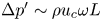 $\Delta p' \sim \rho u_c \omega L$, is of order
  $(h_o-h)/h_o \sim \varepsilon$. The problem is described with use of Cartesian coordinates with longitudinal and transverse components
  $(x,y)$ scaled with
  $L$ and
  $h_{o}$, respectively, and accompanying velocity components
  $(u,v)$ scaled with
  $u_{c}$ and
  $u_{c}h_{o}/L$, the latter scaling following from continuity. The pressure variations are scaled with
  $\rho u_c \omega L$ to give the variable
  $p$ and the membrane displacement is written in the dimensionless form
 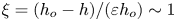 $\xi =(h_{o}-h)/(\varepsilon h_{o}) \sim 1$. The superscripts
  $o$ and
  $c$ are used to denote the values of
  $u$,
$u$,  $v$ and
  $p$ in the channel and in the cavity, respectively.
2.2. Dimensionless equations
In the slender-flow approximation, which applies with small relative errors of order  $(h_{o}/L)^{2}$, viscous stresses associated with longitudinal velocity derivatives can be neglected in the first approximation along with transverse pressure differences, so that
  $p=p(x,t)$ with
  $t=\omega t'$. The problem reduces to the integration of
 \begin{equation} \dfrac{\partial u}{\partial x}+\dfrac{\partial v}{\partial y}=0\quad\text{and}\quad\dfrac{\partial u}{\partial t}+\varepsilon\left(u\frac{\partial u}{\partial x}+v\frac{\partial u}{\partial y}\right)={-}\dfrac{\partial p}{\partial x}+\dfrac{1}{\alpha^{2}}\dfrac{\partial^{2}u}{\partial y^{2}}, \end{equation}
for  $0 \le x \le 1$ with boundary conditions at the lateral boundaries
 \begin{equation} u^{o}=v^{o}=0, \quad {\rm at} \ y=1 \quad {\rm and} \quad u^{o}=v^{o}-\partial \xi/\partial t=0, \quad {\rm at}\ y=\varepsilon \xi \end{equation}
for the channel flow and
 \begin{equation} u^{c}=v^{c}=0, \quad {\rm at} \ y={-}H \quad {\rm and} \quad u^{c}=v^{c}-\partial \xi/\partial t=0, \quad {\rm at}\ y=\varepsilon \xi \end{equation}
for the cavity flow, where  $H=h_c/h_o$ denotes the dimensionless cavity width.
Since the flow rate takes the prescribed value  $\int _0^1 u^o \,{\rm d} y=\cos t$ upstream and downstream from the cavity, the velocity in the channel for
  $x<0$ and
  $x>1$ reduces to the familiar Womersley solution
 \begin{equation} u^o=\mathrm{Re}\left\{\frac{1-\cosh[\alpha \sqrt{\mathrm{i}}(y-1/2)]/\cosh(\alpha \sqrt{\mathrm{i}}/2)}{1-\tanh(\alpha \sqrt{\mathrm{i}}/2)/(\alpha \sqrt{\mathrm{i}}/2)}\mathrm{e}^{\mathrm{i} t}\right\} \quad {\rm with} \ v^o=0. \end{equation}
For  $0< x<1$, the local flow rate
  $Q^o(x,t)=\int _{\varepsilon \xi }^1 u^o \,{\rm d} y$, different in general from the prescribed boundary value
  $Q^o=\cos t$, is related to the flow rate in the cavity
  $Q^c=\int _{-H}^{\varepsilon \xi } u^{c} \,\text {d}y$ by
 \begin{equation} \frac{\partial}{\partial x} \left(\int_{\varepsilon \xi}^1 u^{o} \,{\rm d} y\right)={-}\frac{\partial}{\partial x} \left(\int_{{-}H}^{\varepsilon \xi} u^{c}\, {\rm d} y\right)=\frac{\partial \xi}{\partial t}, \end{equation}
obtained by integrating the first equation in (2.5a,b). Using the known boundary values
 \begin{equation} Q^o=\int_{\varepsilon \xi}^{1}u^{o}\,\text{d}y=\cos t \quad {\rm and} \quad Q^c=\int_{{-}H}^{\varepsilon \xi}u^{c}\,\text{d}y=0 \quad {\rm at} \ x=0,1 \end{equation}
in integrating (2.9) yields
 \begin{equation} \int_{{-}H}^{\varepsilon \xi} u^{c} \,{\rm d} y=\cos t-\int_{\varepsilon \xi}^1 u^{o} \,{\rm d}y={-}\int_0^x \frac{\partial \xi}{\partial t} \,{\rm d}\kern 0.06em \hat{x}, \end{equation}
where  $\hat {x}$ represents a dummy integration variable. The above expression reveals that the flow rate in the cavity is balanced by a reverse flow in the channel of the same magnitude, so that the sum of both remains equal to the Womersley value
  $\cos t$.
The cavity and channel motions are coupled through the elastic equation
 \begin{equation} \mathcal{T} \frac{\partial^2 \xi}{\partial x^2}=p^{o}-p^{c},\end{equation}
with the membrane deformation  $\xi$ satisfying the boundary conditions
 \begin{equation} \xi=0, \quad {\rm at} \ x=0,1 \end{equation}
along with the integral constraint
 \begin{equation} \int_0^1 \xi \,{\rm d}\kern0.06em x=0, \end{equation}
consistent with (2.2). In the elastic equation, the factor
 \begin{equation} \mathcal{T}=\frac{T h_o}{\rho \omega^2 L^4} \end{equation}
is a dimensionless membrane tension.
2.3. Governing parameters and solution procedure
Besides the geometrical parameter  $H=h_c/h_o$, the problem formulated above displays three parameters, namely the Womersley number
  $\alpha$ defined in (2.1), the dimensionless stroke length
  $\varepsilon$ defined in (2.3) and the dimensionless membrane tension
  $\mathcal {T}$ defined in (2.15). The canonical model is designed to represent the dynamical behaviour encountered in syringomyelia syrinxes, with transverse sizes
  $h_c$ comparable to, or somewhat larger than, the thickness of the surrounding SAS
  $h_o \sim 1\unicode{x2013}4$ mm, so that the focus below is on order-unity values of
  $H$. For cardiac-driven flow, the angular frequency is of order
  $\omega =2{\rm \pi}$ s
 $^{-1}$ (i.e. assuming a cardiac rate of 60 beats per minute), so that the resulting Womersley number typically lies in the range
  $3 \lesssim \alpha \lesssim 12$, as follows from (2.1) when the value
  $\nu \simeq 0.7 \times 10^{-6}\,{\rm m}^2\,{\rm s}^{-1}$ of the CSF kinematic viscosity at normal body temperature is used in the evaluation. With CSF peak velocities of the order of a few centimetres per second in the cervical SAS and cavity lengths of the order of a few centimetres, the resulting stroke length
  $\varepsilon =u_c/(\omega L)$ is moderately small (i.e.
  $\varepsilon \simeq 0.1\unicode{x2013}0.2$), motivating an asymptotic description leveraging the limit
  $\varepsilon \ll 1$. The value of the dimensionless membrane tension
  $\mathcal {T}$ must be selected to represent the dynamical deformation of the spinal cord tissue. The previous in vivo measurements of Vinje et al. (Reference Vinje, Brucker, Rognes, Mardal and Haughton2018) reveal velocities in the syrinx that are comparable with those in the SAS, which in our model problem require membrane displacements
  $\xi$ of order unity (e.g. see (2.11)) and corresponding values of
  $\mathcal {T}$ also of order unity, according to (2.12). It appears therefore reasonable to explore the distinguished limit
  $\mathcal {T} \sim 1$ in which the channel and cavity flows display two-way coupling. Note that this limit arises when the characteristic wavelength
  $\lambda _{e}=[(T h_{o})/(\rho \omega ^{2})]^{1/4}$ of the elastic membrane deformations associated with a forcing frequency
  $\omega$ is comparable with the cavity length
  $L$.
$L$.
In the following quantitative description, pertaining to general order-unity values of  $H$,
$H$,  $\alpha$ and
  $\mathcal {T}$ and asymptotically small values of
  $\varepsilon$, all dependent variables are expressed as expansions in powers of
  $\varepsilon \ll 1$ (e.g.
  $u^{o}=u_{0}^{o}+\varepsilon u_{1}^{o}+\cdots$), leading to a hierarchy of problems that can be solved sequentially. The leading-order terms in the expansions, satisfying a linear problem, are purely harmonic, so that their cycle-averaged values are identically zero. In contrast, the first-order velocity corrections contain a non-zero steady-streaming component involving a non-zero transmembrane pressure difference, to be determined below. To facilitate the development, it is convenient to replace
  $y$ with a normalized transverse coordinate
  $\eta$ defined as
 \begin{equation} \eta=\frac{y-\varepsilon\xi}{1-\varepsilon\xi} \text{(channel)}\quad\text{and}\quad\eta={-}\frac{y-\varepsilon\xi}{H+\varepsilon\xi} \text{(cavity)}, \end{equation}
such that  $\eta =0$ at the membrane and
  $\eta =1$ at the opposite flat wall.
3. Leading-order oscillatory motion
3.1. Velocity field
The leading-order solution can be expressed in the form
 \begin{equation} (u_{0}^{o},v_{0}^{o},p_{0}^{o},u_{0}^{c},v_{0}^{c},p_{0}^{c},\xi_{0})=\mathrm{Re}[(U,V,P,\tilde{U},\tilde{V},\tilde{P},\chi)\mathrm{e}^{\mathrm{i} t}] \end{equation}
in terms of the complex functions  $U(x,\eta )$,
  $V(x,\eta )$,
  $P(x)$,
  $\tilde {U}(x,\eta )$,
  $\tilde {V}(x,\eta )$,
  $\tilde {P}(x)$ and
  $\chi (x)$. In the channel, the solution reduces to the integration of
 \begin{equation} \dfrac{\partial U}{\partial x}+\dfrac{\partial V}{\partial\eta}=0\quad\text{and}\quad\dfrac{1}{\alpha^{2}}\dfrac{\partial^{2}U}{\partial\eta^{2}}-\mathrm{i} U=\dfrac{\text{d}P}{{\rm d}\kern0.06em x}, \end{equation}
with boundary conditions  $U=V=0$ at
  $\eta =1$,
  $U=V-i\chi =0$ at
  $\eta =0$, as follows at this order from (2.5a,b) and (2.6a,b), with the reduced velocity satisfying the additional constraint
  $\int _{0}^{1}U\,\text {d}\eta =1$ at
  $x=0,1$, consistent with (2.10a,b). Integrating the second equation in (3.2a,b) with
  $U=0$ at
  $\eta =(0,1)$ yields
 \begin{equation} U=\mathrm{i} \left\{1-\dfrac{\cosh\left[\varLambda\left(2\eta-1\right)\right]}{\cosh\varLambda}\right\}\dfrac{\text{d}P}{{\rm d}\kern0.06em x}, \end{equation}
where  $\varLambda =\alpha \sqrt {\mathrm {i}}/2$. The expression for
  $U$ can be used in the first equation in (3.2a,b) to provide
 \begin{equation} V={-}\mathrm{i} \left\{\eta-1-\dfrac{\sinh\left[\varLambda\left(2\eta-1\right)\right]-\sinh\varLambda}{2\varLambda\cosh\varLambda}\right\}\dfrac{\text{d}^{2}P}{{\rm d}\kern0.06em x^{2}} \end{equation}
upon integration with use of  $V=0$ at
  $\eta =1$.
The same integration procedure can be applied to the cavity flow to give
 \begin{gather} \tilde{U}=\mathrm{i} \left\{1-\frac{\cosh[H\varLambda\left(2\eta-1\right)]}{\cosh\left(H\varLambda\right)}\right\}\dfrac{\text{d}\tilde{P}}{{\rm d}\kern0.06em x}, \end{gather}
 \begin{gather}\tilde{V}=\mathrm{i} H \left\{\eta-1-\frac{\sinh[H\varLambda\left(2\eta-1\right)]-\sinh\left(H\varLambda\right)}{2H\varLambda\cosh\left(H\varLambda\right)}\right\} \dfrac{\text{d}^{2}\tilde{P}}{{\rm d}\kern0.06em x^{2}}. \end{gather}
The velocity profiles (3.3) and (3.5) can be used to evaluate the integrals
 \begin{equation} \int_0^1 U \,{\rm d}\eta=\frac{1}{\beta} \dfrac{\text{d}P}{{\rm d}\kern0.06em x} \quad {\rm and} \quad H \int_0^1 \tilde{U} \,{\rm d}\eta=\frac{1}{\tilde{\beta}} \dfrac{\text{d}\tilde{P}}{{\rm d}\kern0.06em x}, \end{equation}
which enter in the computation of the leading-order oscillatory flow rates
 \begin{align} Q^o_0=\int_0^1 u_0^o \,{\rm d} y=\mathrm{Re}\left(\int_0^1 U {\rm d}\eta \, \mathrm{e}^{\mathrm{i} t} \right)\quad {\rm and} \quad Q^c_0=\int_{{-}H}^0 u_0^c \,{\rm d} y=\mathrm{Re}\left(H \int_0^1 \tilde{U}\, {\rm d}\eta \, \mathrm{e}^{\mathrm{i} t} \right), \end{align}
with
 \begin{equation} \beta={-}{\rm i}\left[1-\varLambda^{{-}1}\tanh\varLambda\right]^{{-}1} \quad {\rm and} \quad \tilde{\beta}={-}{\rm i}\left[H-\varLambda^{{-}1}\tanh(H\varLambda)\right]^{{-}1}. \end{equation}
As can be seen from (3.3) and (3.4), when the pressure gradient takes the uniform unperturbed value  ${\rm d}P/{\rm d}\kern0.06em x=\beta$, the leading-order velocity in the channel
  $(u^o_0,v^o_0)=\mathrm {Re}[(U,V)\mathrm {e}^{\mathrm {i} t}]$ reduces to the familiar Womersley solution (2.8) existing for
  $x<0$ and
  $x>1$.
3.2. Membrane deformation
The pressure distributions in the channel and in the cavity  $P(x)$ and
  $\tilde {P}(x)$, which complete the determination of the flow at this order, are related to the membrane deformation by
 \begin{equation} \dfrac{\text{d}^{2}P}{{\rm d}\kern0.06em x^{2}}=\mathrm{i} \beta \chi \quad \text{and} \quad \dfrac{\text{d}^{2}\tilde{P}}{{\rm d}\kern0.06em x^{2}}={-}\mathrm{i} \tilde{\beta} \chi, \end{equation}
as follows from using the boundary conditions  $V=\tilde {V}=\mathrm {i} \chi$ at
  $\eta =0$ in (3.4) and (3.6). Their values are coupled through
 \begin{equation} \mathcal{T} \frac{{\rm d}^2 \chi}{{\rm d}\kern0.06em x^2}=P-\tilde{P}, \end{equation}
obtained at leading-order from (2.12). Differentiating twice the above equation followed by substitution of (3.7a,b) provides the boundary-value problem
 \begin{equation} \dfrac{\text{d}^{4}\chi}{{\rm d}\kern0.06em x^{4}}-\frac{\mathrm{i} (\beta+\tilde{\beta})}{\mathcal{T}}\chi=0\quad\text{with}\ \left\{ \begin{array}{@{}r} \text{d}^{3}\chi/{\rm d}\kern0.06em x^{3}=\beta/\mathcal{T}\\ \chi=0 \end{array}\right.\quad\text{at}\ x=\left(0,1\right) \end{equation}
for the membrane displacement  $\chi$. The boundary condition involving the third derivative follows from imposing the conditions
  ${\rm d} P/{\rm d}\kern0.06em x-\beta ={\rm d} \tilde {P}/{\rm d}\kern0.06em x=0$ at
  $x=0,1$, corresponding to
  $\int _{0}^{1}U\,\text {d}\eta -1=\int _{0}^{1}\tilde {U}\,\text {d}\eta =0$. The deformation satisfies
  $\int _0^1 \chi \,{\rm d}\kern0.06em x=0$, as can be readily verified by performing a first quadrature of (3.12).
The solution to (3.12) can be written as
 \begin{align} \chi=\dfrac{\beta}{\mathcal{T}} \left\{\dfrac{\sin\left(\dfrac{\gamma}{2\mathcal{T}^{1/4}}\right)\sinh\left[\dfrac{\gamma}{\mathcal{T}^{1/4}}\left(x-\dfrac{1}{2}\right)\right]-\sinh\left(\dfrac{\gamma}{2\mathcal{T}^{1/4}}\right)\sin\left[\dfrac{\gamma}{\mathcal{T}^{1/4}}\left(x-\dfrac{1}{2}\right)\right]}{\left(\dfrac{\gamma}{\mathcal{T}^{1/4}}\right)^{3} \left[\sinh\left(\dfrac{\gamma}{2\mathcal{T}^{1/4}}\right)\cos\left(\dfrac{\gamma}{2\mathcal{T}^{1/4}}\right)+\cosh\left(\dfrac{\gamma}{2\mathcal{T}^{1/4}}\right)\sin\left(\dfrac{\gamma}{2\mathcal{T}^{1/4}}\right)\right]}\right\}, \end{align}
where 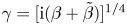 $\gamma =[\mathrm {i} (\beta +\tilde {\beta })]^{1/4}$. The above expression can be used in (3.7a,b) to obtain
  $\text {d}^2 P/\text {d}\kern 0.06em x^2$ and
  $\text {d}^2 \tilde {P}/\text {d}\kern 0.06em x^2$, needed in (3.4) and (3.6). On the other hand, integration of (3.7a,b) subject to
  $\text {d}P/\text {d}\kern 0.06em x-\beta =\text {d}\tilde {P}/\text {d}\kern 0.06em x=0$ at
  $x=0$ provides the pressure gradients required in (3.3) and (3.5), resulting in
 \begin{equation} \frac{1}{\beta} \dfrac{\text{d}P}{{\rm d}\kern0.06em x}-1={-}\frac{1}{\tilde{\beta}} \dfrac{\text{d}\tilde{P}}{{\rm d}\kern0.06em x}=\mathrm{i}\int_0^x\chi\,\text{d}\kern 0.06em \hat{x} \end{equation}
with
 $$\begin{align} &\mathrm{i} \int_0^x\chi\,\text{d}\kern 0.06em \hat{x}=\frac{\beta}{\beta+\tilde{\beta}} \left\{ \coth[\gamma/(2\mathcal{T}^{1/4})]+\cot[\gamma/(2\mathcal{T}^{1/4})]\right\}^{{-}1} \nonumber\\ &\times \left(\dfrac{\cosh\left[\dfrac{\gamma}{\mathcal{T}^{1/4}}\left(x-\dfrac{1}{2}\right)\right]\!-\!\cosh\left(\dfrac{\gamma}{2\mathcal{T}^{1/4}}\right)}{\sinh[\gamma/(2\mathcal{T}^{1/4})]}+ \dfrac{\cos\left[\dfrac{\gamma}{\mathcal{T}^{1/4}}\left(x-\dfrac{1}{2}\right)\right]\!-\!\cos\left(\dfrac{\gamma}{2\mathcal{T}^{1/4}}\right)}{\sin[\gamma/(2\mathcal{T}^{1/4})]}\right), \end{align}$$
the latter entering when using (3.7a,b) and (3.7a,b) for the determination of the flow rates
 \begin{equation} \int_{{-}H}^0 u_0^c \,{\rm d} y=\cos t-\int_0^1 u_0^o \,{\rm d} y={-}\mathrm{Re}\left(\mathrm{i} \int_0^x\chi\,\text{d}\kern 0.06em \hat{x} \, \mathrm{e}^{\mathrm{i} t} \right). \end{equation}
Note that the last equation corresponds to the leading-order form of (2.11).
3.3. Oscillatory motion
The closed-form expressions derived above can be used to investigate the main features of the FSI oscillatory dynamics and its parametric dependences. We begin by plotting in figures 3(b,e,h) and 3(c,f,i) snapshots of streamlines and membrane displacement at two different instants of time corresponding to a configuration with  $\alpha =5$ and
  $H=1$. Colour contours are used to represent the associated vorticity, which in the slender-flow approximation reduces to
  $-\partial u_0/\partial y$. The accompanying temporal variations of the leading-order flow rates
  $Q_0^c=\int _{-H}^0 u_0^c \,{\rm d} y$ and
  $Q_0^o=\int _0^1 u_0^o \,{\rm d} y$ at the canal middle section
  $x=0.5$ are shown in figure 3(a,d,g). The computations reveal, in particular, that the value of
  $\mathcal {T}$ needs to be much smaller than unity to induce significant membrane displacements (and therefore significant motion in the cavity). For example, for
  $\mathcal {T}=0.05$, the case shown in figure 3(g–i), the membrane displacement is limited to values
  $\xi _0 <0.1$ and the fluid remains nearly stagnant in the cavity, associated departures from Womersley flow in the channel being correspondingly small.

Figure 3. Oscillatory flow for a configuration with  $\alpha =5$,
  $H=1$ and
  $\mathcal {T}=$ (a–c)
  $0.0001$, (d–f)
  $0.01$ and (g–i)
  $0.05$. (a,d,h) The variation with time of the channel (blue) and cavity (red) flow rates
  $Q_0^o=\int _0^1 u_0^o \,{\rm d} y$ and
  $Q_0^c=\int _{-H}^0 u_0^c \,{\rm d} y$ at
  $x=0.5$ evaluated using (3.16). (b,e,h,c,f,i) Streamlines and colour contours of vorticity at
  $t={\rm \pi} /4$ and
  $t={\rm \pi}$ along with the corresponding membrane displacement
  $\xi _0$. To facilitate comparisons, a fixed constant streamline spacing of
  $\delta \psi _0=0.05$ has been used in representing the streamlines, with the stream function
  $\psi _0$ computed using
  $\partial \psi _0/\partial y=u_0$ and
  $\partial \psi _0/\partial x=-v_0$.
The limited membrane displacement found for  $\mathcal {T} \sim 1$ can be attributed to the smallness of the term in curly brackets in the general expression (3.13). This can be seen more clearly by considering the limit of very stiff membranes
  $\mathcal {T} \gg 1$, in which one can readily integrate (3.12) to give the approximate result
 \begin{equation} \chi\simeq\dfrac{\beta}{\mathcal{T}}\dfrac{x}{6}\left(x-\dfrac{1}{2}\right)\left(x-1\right) \quad \text{for} \ \mathcal{T} \gg 1. \end{equation}
Straightforward evaluation reveals that the maximum displacement in this limit, reached at  $x=1/2\pm \sqrt {3}/6$, is
  $\chi \simeq 8.02 \times 10^{-3} \beta /\mathcal {T}$, with the small numerical factor being consistent with the results shown in the figure.
In contrast to the case  $\mathcal {T}=0.05$, the configurations with
  $\mathcal {T}=10^{-4}$ and
  $\mathcal {T}=10^{-2}$, shown in figures 3(a–c) and 3(d–f), respectively, show velocities in the cavity that are comparable with those in the channel. The streamlines in all plots have been represented using the same values of the stream function, so that their inter-spacing characterizes the local flow speed. The comparison of the streamlines in figures 3(a–c) and 3(d–f) reveals that the flow patterns become more complicated as the membrane becomes more flexible for decreasing values of
  $\mathcal {T}$. In interpreting this result, it is worth recalling that the dimensionless membrane tension can be expressed as
  $\mathcal {T}=(\lambda _e/L)^4$ in terms of the characteristic elastic wavelength
  $\lambda _{e}=[(Th_{o})/(\rho \omega ^{2})]^{1/4}$, so that the number of membrane undulations increases for decreasing values of
  $\mathcal {T}$, driving separate regions of recirculating flow.
The dynamics of the sloshing motion induced in the cavity is characterized in figure 4 by plotting the temporal variation over a cycle of the tightly coupled cavity deformation  $\xi _0$, flow rate
  $Q_o^c=\int _{-H}^0 u_0^c \,{\rm d} y$ and oscillatory transmembrane pressure
  $p_0^c-p_0^o=\mathrm {Re}[(\tilde {P}-P)\mathrm {e}^{\mathrm {i} t}]$, with
  $\tilde {P}-P$ evaluated from (3.11) by straightforward double differentiation of (3.13). As can be expected from (3.11) and (3.16), the membrane displacement is in phase with
  $p_0^c-p_0^o$, while the flow rate is in quadrature. At the initial time
  $t={\rm \pi} /4$ selected in the figure, the membrane is practically flat and the transmembrane pressure difference is very small. The fluid, with an initially negative flow rate, moves upstream, deforming the membrane and inducing a negative pressure gradient that slows down the motion, so that the velocity vanishes when the deformation reaches its maximum at
  $t=3{\rm \pi} /4$. The flow reverses for
  $t>3{\rm \pi} /4$, with the negative pressure gradient driving the flow downstream. A nearly flat membrane with negligible transmembrane pressure gradient is found for
  $t=5{\rm \pi} /4$ as the flow rate reaches its peak positive value. The sloshing behaviour is replicated over the second half of the cycle following the expected sinusoidal pattern. In view of figure 3(a–c), it can be anticipated that the sloshing-flow structure becomes more complicated as the elastic wavelength becomes much smaller than
  $L$ for decreasing values of
  $\mathcal {T}$, that being the case investigated below.

Figure 4. The variation with time of (a) the membrane displacement  $\xi _0$, (b) cavity flow rate
  $Q_o^c=\int _{-H}^0 u_o^c \,{\rm d} y$ and (c) oscillatory transmembrane pressure difference
  $p_0^c-p_0^o$ for a cavity with
  $\alpha =5$,
  $H=1$ and
  $\mathcal {T}=0.01$.
3.4. Very flexible membranes
For values of  $\mathcal {T}$ smaller than those considered in figure 3, the membrane undulations, of larger amplitude for decreasing
  $\mathcal {T}$, remain mostly confined to near-edge regions scaling with the elastic-wave wavelength. Illustrative results pertaining to this limit of very flexible membranes are shown in figure 5, including instantaneous membrane shapes at selected times and associated cavity flow rates.

Figure 5. The streamwise variation of (a–c) the membrane displacement  $\xi _0$ and (d–f) cavity flow rate
  $Q_0^c=\int _{-H}^0 u_0^c \,{\rm d} y$ at (a,d)
  $t=0$, (b,e)
  $t = {\rm \pi}/4$ and (c,f)
  $t = {\rm \pi}/2$ for
  $\alpha =3$,
  $H=2$ and
  $\mathcal {T}=(10^{-3},10^{-5},10^{-8}$).
The structure that emerges can be investigated by exploring the asymptotic limit  $\mathcal {T} \ll 1$, wherein (3.12) reduces to
  $\chi =0$ while (3.11) yields
  $P=\tilde {P}$, so that the fluid moves in the channel and in the cavity under the action of the same pressure gradient. This solution fails near the edges of the membrane, in two boundary regions
  $x\sim \mathcal {T}^{1/4}\ll 1$ and
  $(1-x)\sim \mathcal {T}^{1/4}\ll 1$, where
  $\chi \sim \mathcal {T}^{-1/4}\gg 1$ and
  $P\sim \tilde {P}\sim \mathcal {T}^{1/4}\ll 1$ whose solution determines the pressure gradient driving the uniform flow rate in the central region. Introducing the rescaled variables
  $\zeta =x/\mathcal {T}^{1/4}$ (replaced by
  $\zeta =(1-x)/\mathcal {T}^{1/4}$ in the description of the right-hand-side edge region),
  $\chi _e=\mathcal {T}^{1/4}\chi$,
  $P_e=P/\chi ^{1/4}$ and
  $\tilde {P}_e=\tilde {P}/\chi ^{1/4}$ leads to the modified boundary-value problem
 \begin{equation} \dfrac{\text{d}^{4}\chi_e}{\text{d}\zeta^{4}}-\gamma^{4}\chi_e=0\quad\left\{ \begin{array}{@{}ll} \dfrac{\text{d}^{3}\chi_e}{\text{d}\zeta^{3}}-\beta=\chi_e=0, & \text{at}\ \zeta=0,\\ \chi_e\rightarrow0, & \text{as}\ \zeta\rightarrow\infty, \end{array}\right. \end{equation}
which can be integrated to give
 \begin{equation} \chi_e=\dfrac{\beta}{\gamma^{3}\left(1-i\right)}\left(\mathrm{e}^{\text{i}\gamma\zeta}-\mathrm{e}^{-\gamma\zeta}\right).\end{equation}
Without loss of generality, in writing the above expression we have used the complex root  $\gamma =[\mathrm {i} (\beta +\tilde {\beta })]^{1/4}$ lying in the first quadrant, so that
  ${\rm e}^{{\rm i}\gamma \zeta }\rightarrow 0$ and
  $e^{-\gamma \zeta }\rightarrow 0$ as
  $\zeta \rightarrow \infty$. Substituting (3.19) into the rescaled form of (3.14) and (3.16) yields
 \begin{equation} \frac{1}{\beta}\dfrac{\text{d}P_e}{{{\text{d}\zeta}}}-1={-}\frac{1}{\tilde{\beta}} \dfrac{\text{d}\tilde{P}_e}{{{\text{d}\zeta}}}=\frac{\beta}{\beta+\tilde{\beta}} \left(\frac{\mathrm{e}^{-\gamma\zeta}-\mathrm{i} \mathrm{e}^{\text{i}\gamma\zeta}}{1-\mathrm{i}}-1 \right) \end{equation}
and
 \begin{equation} \int_{{-}H}^0 u_0^c \,{\rm d} y=\cos t-\int_0^1 u_0^o \,{\rm d} y={-}\mathrm{Re}\left[\frac{\beta}{\beta+\tilde{\beta}} \left(\frac{\mathrm{e}^{-\gamma\zeta}-\mathrm{i} \mathrm{e}^{\text{i}\gamma\zeta}}{1-\mathrm{i}}-1 \right) \mathrm{e}^{\mathrm{i} t} \right] \end{equation}
for the pressure gradients and flow rates in the near-edge regions. The result can be evaluated as  $\zeta \rightarrow \infty$ to obtain the uniform values
 \begin{equation} \dfrac{\text{d}P}{{{{\rm d}\kern0.06em x}}}=\dfrac{\text{d}\tilde{P}}{{{{\rm d}\kern0.06em x}}}=\frac{\beta\tilde{\beta}}{\beta+\tilde{\beta}} \end{equation}
and
 \begin{equation} \int_{{-}H}^0 u_0^c \,{\rm d} y=\cos t-\int_0^1 u_0^o \,{\rm d} y=\mathrm{Re}\left(\frac{\beta \mathrm{e}^{\mathrm{i} t}}{\beta+\tilde{\beta}}\right) \end{equation}
that prevail away from the edge regions.
3.5. Parametric dependences of the flow rate
As can be inferred from (3.16), the parametric dependences of the oscillating flow rate in the cavity (and, correspondingly, of the departures from Womersley flow in the channel) are embodied in the function  $\mathrm {i} \int _0^x \chi \, {\rm d}\kern0.7pt \hat {x}$ given in (3.15). A measure of the induced motion is provided by the local amplitude of the oscillating flow rate across the central section
  $x=1/2$ of the cavity, given by the modulus
  $|\!\int _0^{1/2}\chi \,\text {d}\kern 0.06em x|$, which is also proportional to the corresponding stroke volume
  $\int _t^{t+2{\rm \pi} } |Q_0^c(1/2,t)| \,{\rm d}t/(2{\rm \pi} )=(2/{\rm \pi} ) |\!\int _0^{1/2}\chi \,\text {d}\kern 0.06em x|$. The variation of
  $|\!\int _0^{1/2}\chi \,\text {d}\kern 0.06em x|$ with
  $\mathcal {T}$ is represented in figure 6 for different values of
  $H$ and
  $\alpha$.

Figure 6. The variation with  $\mathcal {T}$ of the amplitude of the oscillating flow rate
  $|\!\int _0^{1/2}\chi \,\text {d}\kern 0.06em x|$ across the central section
  $x=1/2$ of the cavity for
  $\alpha =3$ (a) and
  $\alpha =6$ (b) and four different values of
  $H=(0.5,1,2,\infty )$. The inset in (a) represents an expanded view of the curves as they merge for increasing
  $\mathcal {T}$ while that in (b) gives the variation with
  $\alpha$ of the peak value of
  $|\!\int _0^{1/2}\chi \,\text {d}\kern 0.06em x|$ for three different values of
  $H$.
$H$.
The curves reproduce the trends previously identified. In particular, the motion is very limited for values of  $\mathcal {T} \gtrsim 0.1$, when the flow rate becomes independent of
  $H$, as seen in the inset of figure 6(a), with a value that decays for
  $\mathcal {T} \gg 1$ according to
  $|\!\int _0^{1/2}\chi \,\text {d}\kern 0.06em x|=|\beta |/(384 \mathcal {T})$, a result derived with use of (3.17). In the opposite limit
  $\mathcal {T} \ll 1$ of very flexible membranes, the flow-rate amplitude approaches the constant value
  $|\!\int _0^{1/2}\chi \,\text {d}\kern 0.06em x|=|\beta /(\beta +\tilde {\beta })|$, larger for larger
  $H$, with
  $|\!\int _0^{1/2}\chi \,\text {d}\kern 0.06em x|=0.5$ when
  $\beta =\tilde {\beta }$ for
  $H=1$. The flow rate in the central part of the cavity becomes maximum for an intermediate value of
  $\mathcal {T}$ lying in the range
  $10^{-3} < \mathcal {T} < 10^{-2}$, with the peak becoming more pronounced with increasing
  $\alpha$, as shown in the inset of figure 6(b). Between their peak values and the asymptotic values approached as
  $\mathcal {T} \rightarrow 0$, the curves in figure 6 display oscillations of decreasing amplitude, which are related to the development of an increasing number of membrane undulations as the cavity length
  $L$ becomes larger than the elastic wavelength
  $\lambda _e$ for decreasing values of
  $\mathcal {T}=(\lambda _e/L)^4$.
3.6. Effects of complex waveform
The rapid decay from its peak value experienced by  $|\!\int _0^{1/2}\chi \,\text {d}\kern 0.06em x|$ as
  $\mathcal {T}$ increases, more prominent for larger
  $\alpha$, is indicative of a strong frequency dependence of the flow rate induced in the cavity. As indicated by the plots in figure 6, for intermediate values of
  $\mathcal {T} \sim 10^{-2}$, increasing the frequency (i.e. reducing the value of
  $\mathcal {T} \propto \omega ^{-2}$ and increasing the value of
  $\alpha \propto \omega ^{1/2}$) may promote significantly the motion in the cavity, with implications concerning the characteristics of the oscillatory flow in syringomyelia syrinxes, an aspect of the flow investigated below.
The typical waveform of the cardiac-driven flow rate  $Q'$ at the entrance of the spinal canal has a non-sinusoidal waveform, so that the Fourier decomposition of the signal has multiple harmonics of frequency
  $n \omega$. For instance, a Fourier analysis of the periodic flow rate corresponding to a Chiari patient, shown in figure 7(a), obtained by rescaling PC MRI velocity measurements reported by Vinje et al. (Reference Vinje, Brucker, Rognes, Mardal and Haughton2018), yields
 \begin{equation} Q'/\langle|Q'|\rangle=\sum_{n=1}^\infty \mathrm{Re} \left(A_n \mathrm{e}^{\mathrm{i} n t}\right), \end{equation}
where  $A_n$ are complex constants of order unity, with
  $A_1=0.2765 - 1.4686\mathrm {i}$,
  $A_2=0.0206- 0.6748 \mathrm {i}$ and
  $A_3=-0.1203- 0.2222\mathrm {i}$ for the first three modes. Here, we have normalized the flow rate with its average amplitude
  $\langle |Q'|\rangle =\int _0^{2{\rm \pi} } |Q'| \,{\rm d}t/(2{\rm \pi} )$. For comparison, figure 7(a) includes the purely sinusoidal case
  $Q'/\langle |Q'|\rangle =({\rm \pi} /2) \sin (t)$ (i.e.
  $A_1=-({\rm \pi} /2) \mathrm {i}$ with
  $A_n=0$ for
  $n>1$).

Figure 7. (a) Comparison of the dimensionless flow rate at the entrance of the spinal canal measured by cardiac-gated PC MRI (adapted from Vinje et al. Reference Vinje, Brucker, Rognes, Mardal and Haughton2018) (solid curve) with the sinusoidal signal  $Q'/\langle |Q'|\rangle =({\rm \pi} /2) \sin (t)$ (dashed curve). The two waveforms are used to determine the response of the cavity flow for a configuration with
  $\alpha =5$,
  $\mathcal {T}=0.02$ and two different cavity widths
  $H=1$ (red curves) and
  $H=4$ (blue curves), including (b) the variation with time of the cavity flow rate
  $Q_0^c=\int _{-H}^0 u_0^c \,{\rm d} y$ at
  $x=1/2$ determined from (3.25) and (c) the streamwise variation of the transmural steady pressure difference
  $\langle\, p_{1}^{c}\rangle -\langle\, p_{1}^{o}\rangle$ computed from (4.28). For consistency with (a), the solid/dashed curves in (b,c) are computed with the complex/sinusoidal channel-flow waveforms.
The analysis given above, pertaining to a simple sinusoidal flow rate, can be readily extended to account for the presence of the different harmonics, leading to the flow-rate expressions
 \begin{equation} \int_{{-}H}^0 u_0^c \,{\rm d} y=\sum_{n=1}^\infty \mathrm{Re} \left(A_n \mathrm{e}^{\mathrm{i} n t}\right)-\int_0^1 u_0^o \,{\rm d} y={-}\mathrm{Re}\left(\sum _{n=1}^\infty A_n \mathrm{i} \int_0^x\chi_n\, \text{d}\kern 0.06em \hat{x} \, \mathrm{e}^{\mathrm{i} n t} \right), \end{equation}
with  $u_c=\langle |Q'|\rangle /h_o$ used as characteristic velocity in scaling the problem. The value of
  $\mathrm {i} \int _0^x\chi _n\, \text {d}\kern0.7pt\hat {x}$, measuring the amplification of a specific mode
  $n$, can be determined from the general expression (3.15) by simply replacing
  $\mathcal {T}$ with
  $\mathcal {T}/n^2$ and evaluating
  $\beta$,
  $\tilde {\beta }$ and
  $\gamma =[\mathrm {i}(\beta +\tilde {\beta })]^{1/4}$ with use of
  $n^{1/2} \alpha$ in place of
  $\alpha$.
Bearing in mind the frequency dependence discussed above in connection with figure 6, one may anticipate that, for configurations with  $\mathcal {T}$ sufficiently large, higher-order harmonics
  $n>1$ may have values of the amplification factor
  $\mathrm {i} \int _0^x\chi _n \text {d}\kern0.7pt\hat {x}$ that are larger than those of the fundamental frequency, that being a result of the variation of the frequency-weighted membrane tension
  $\mathcal {T}/n^2$ and Womersley number
  $n^{1/2} \alpha$. As a consequence, although the fundamental mode with frequency
  $\omega$ is clearly dominant in the flow rate at the entrance of the spinal canal
  $Q'$, so that the waveform is nearly sinusoidal, as shown in figure 7(a), the motion induced in the syrinx may exhibit pronounced oscillations at higher frequencies
  $n \omega$. As previously discussed in the introduction, such dynamics has been observed in in vivo non-invasive measurements performed in syringomyelia patients both before and after craniovertebral decompression (Vinje et al. Reference Vinje, Brucker, Rognes, Mardal and Haughton2018). In the preoperative study, the flow in the syrinx was found to display three full oscillations per cardiac cycle (i.e. Vinje et al. (Reference Vinje, Brucker, Rognes, Mardal and Haughton2018) report 210 cycles per minute for a heart rate of 73 beats per minute), indicating that the third harmonic
  $n=3$ was dominant. In contrast, two months after surgery, the flow in the syrinx, now reduced in size (i.e. corresponding to a smaller value of
  $H$ in our analysis), exhibited instead two full oscillations per cardiac cycle (i.e. 200 cycles per minute for a heart rate of 97 beats per minute), consistent with the second harmonic
  $n=2$ being dominant instead in the postoperative state.
The results of the simple FSI model developed here can be used to investigate this intriguing behaviour. Results of an illustrative computation are given in figure 7 for a configuration with  $\alpha =5$,
  $\mathcal {T}=0.02$ and two different values of
  $H$. Figure 7(b) shows the waveform of the periodic flow rate
  $Q_0^c=\int _0^{1} u_0^c \,{\rm d} y$ across the cavity middle section
  $x=1/2$ as determined from (3.25) using the sinusoidal flow rate
  $Q'/\langle |Q'|\rangle =({\rm \pi} /2) \sin (t)$ (dashed curves) and using ten modes in the Fourier expansion (3.24) for the spinal canal flow rate represented with the solid curve in figure 7(a) (solid curves). As can be seen, the flow rate induced in the cavity when the channel flow is purely sinusoidal follows the fundamental frequency. In contrast, the cavity-flow response to the complex waveform, of much larger amplitude, exhibits multiple cycles. In particular, it is seen that the curve with
  $H=4$, representative of the preoperative state, exhibits three cycles, in agreement with the previous in vivo observations (Vinje et al. Reference Vinje, Brucker, Rognes, Mardal and Haughton2018). Interestingly, when the width of the cavity is reduced to
  $H=1$, mimicking the reduction in syrinx transverse size that follows surgery, the second harmonic becomes dominant, so that the resulting waveform of the cavity flow rate shows two cycles instead, again in agreement with the observations (Vinje et al. Reference Vinje, Brucker, Rognes, Mardal and Haughton2018). It is remarkable that, while the configuration investigated here is much too simple to enable quantitative predictions to be made, it is still able to reproduce some aspects of the observed in vivo dynamics when the value of
  $\mathcal {T}$ is selected in the appropriate range.
4. Secondary motion
4.1. Steady streaming
The leading-order solution investigated in the preceding section has a zero time average, so that it does not result in a net transmembrane pressure difference. In contrast, the first-order corrections include a steady component, which can be determined by taking the time average of the corresponding governing equations, obtained by collecting terms of order  $\varepsilon$ in (2.5a,b). In the channel, the problem reduces to the integration of
 \begin{equation} \frac{\partial \langle u_1^o \rangle}{\partial x}+\frac{\partial \langle v_1^o \rangle}{\partial \eta}+G\left(x,\eta\right)=0\quad\text{and}\quad\dfrac{1}{\alpha^{2}} \dfrac{\partial^{2}\langle u_1^o \rangle}{\partial\eta^{2}}=\dfrac{\text{d}\left\langle\, p_{1}^{o}\right\rangle }{{\rm d}\kern0.06em x}+F\left(x,\eta\right) \end{equation}
subject to  $\langle u_1^o \rangle =\langle v_1^o \rangle =0$ at
  $\eta =0,1$ and
  $\int _0^1 \langle u_1^o \rangle \,{\rm d}\eta =0$ at
  $x=0,1$, with
  $\langle \dots \rangle =$
 $\int _{t}^{t+2{\rm \pi} } \, {\rm d}t/(2{\rm \pi} )$ representing the time-averaging operator. The steady motion is driven by the effect of convective acceleration and the nonlinear interactions stemming from the deformation of the canal, which enter in the problem through the functions
 $$\begin{gather} G=\left(\eta-1\right)\left\langle \dfrac{\partial\xi_{0}}{\partial x}\dfrac{\partial u_{0}^{o}}{\partial\eta}\right\rangle +\left\langle \xi_{0}\dfrac{\partial v_{0}^{o}}{\partial\eta}\right\rangle \end{gather}$$
and
 $$\begin{gather}F=\left(\eta-1\right)\left\langle \dfrac{\partial\xi_{0}}{\partial t}\dfrac{\partial u_{0}^{o}}{\partial\eta}\right\rangle +\left\langle u_{0}^{o}\dfrac{\partial u_{0}^{o}}{\partial x}\right\rangle +\left\langle v_{0}^{o}\dfrac{\partial u_{0}^{o}}{\partial\eta}\right\rangle -\dfrac{2}{\alpha^{2}}\left\langle \xi_{0}\dfrac{\partial^{2}u_{0}^{o}}{\partial\eta^{2}}\right\rangle. \end{gather}$$
The time averages of products of harmonic functions in the above expressions can be written in terms of  $U$,
$U$,  $V$ and
  $\chi$ with use of the identity
  $\langle \mathrm {Re}(\mathrm {e}^{\mathrm {i} t} A) \, \mathrm {Re}(\mathrm {e}^{\mathrm {i} t} B) \rangle = \mathrm {Re}(A B^*)/2$, which applies to any generic time-independent complex functions
  $A$ and
  $B$, with the asterisk denoting complex conjugates.
Because of the canal deformation, the cycle-averaged velocity is non-solenoidal, as seen in the first equation of (4.1a,b), resulting in a non-zero flow rate  $\langle Q_1^o \rangle =\int _0^1 \langle u_1^o \rangle \,{\rm d}\eta$. Its value can be determined directly by integrating the continuity equation across the canal with
  $\langle v_1^o \rangle =0$ at
  $\eta =0,1$ to give
 \begin{equation} \frac{\rm d}{{\rm d}\kern0.06em x}\left[\int_0^1 \langle u_1^o \rangle \,{\rm d}\eta -\left\langle \xi_{0}\int_{0}^{1}u_{0}^{o}\,\text{d}\eta\right\rangle\right]=0 \end{equation}
after use is made of integration by parts to reduce  $\int _0^1 G \,{\rm d}\eta$. Since
  $\int _0^1 \langle u_1^o \rangle \,{\rm d}\eta =0$ at
  $x=0,1$, where
  $\xi _0=0$, it follows that
 \begin{equation} \int_0^1 \langle u_1^o \rangle \,{\rm d}\eta=\left\langle \xi_{0}\int_{0}^{1}u_{0}^{o}\,\text{d}\eta\right\rangle.\end{equation}
As seen later in § 4.2, this non-zero flow rate is balanced exactly by that of the Stokes drift, so that the mean Lagrangian motion has a zero flow rate, as it should.
The steady-streaming velocity in the channel is computed by integrating the second equation in (4.1a,b) subject to  $\langle u_1^o \rangle =0$ at
  $\eta =0,1$ to give
 \begin{equation} \langle u_1^o \rangle={-}\alpha^{2}\left[\dfrac{\eta}{2}\left(1-\eta\right)\dfrac{\text{d}\left\langle\, p_{1}^{o}\right\rangle }{{\rm d}\kern0.06em x}+\int_{0}^{\eta}\hat{\eta}F\,\text{d}\hat{\eta} +\eta\left(\int_{\eta}^{1}F\,\text{d}\hat{\eta} -\int_{0}^{1}{\eta}F\,\text{d}{\eta}\right)\right],\end{equation}
which can be used in integrating the first equation in (4.1a,b) with the condition  $\langle v_1^o \rangle =0$ at
  $\eta =0$ to obtain
 $$\begin{align} \langle v_1^o \rangle &=\alpha^{2}\dfrac{\partial}{\partial x}\left[\dfrac{\eta^{2}}{2}\left(\dfrac{1}{2}-\dfrac{\eta}{3}\right)\dfrac{\text{d}\left\langle\, p_{1}^{o}\right\rangle}{{\rm d}\kern0.06em x} -\dfrac{1}{2}\int_{0}^{\eta}F\hat{\eta}^2\,\text{d}\hat{\eta}\right.\nonumber\\ &\quad + \left.\eta\int_{0}^{\eta}F\hat{\eta}\,\text{d}\hat{\eta} +\dfrac{\eta^{2}}{2}\left(\int_{\eta}^{1}F\,\text{d}\hat{\eta} -\int_{0}^{1}F\eta\,\text{d}\eta\right)\right] -\int_{0}^{\eta}G\,\text{d}\hat{\eta}, \end{align}$$
where the pressure gradient is given by
 \begin{equation} \dfrac{\text{d}\left\langle\, p_{1}^{o}\right\rangle }{{\rm d}\kern0.06em x}={-}\frac{12}{\alpha^2} \left\langle \xi_{0}\int_{0}^{1}u_{0}^{o}\,\text{d}\eta\right\rangle - 6 \int_{0}^{1}F\eta\left(1-\eta\right)\,{\rm d}\eta, \end{equation}
as follows from substitution of (4.6) into (4.5). A similar analysis of the cavity flow provides
 \begin{gather} \langle u_1^c \rangle={-}\left(\alpha H\right)^{2}\left[\dfrac{\eta}{2}\left(1-\eta\right)\dfrac{\text{d}\left\langle\, p_{1}^{c}\right\rangle }{{\rm d}\kern0.06em x}+\int_{0}^{\eta}\hat{\eta}\tilde{F}\,\text{d}\hat{\eta} +\eta\left(\int_{\eta}^{1}\tilde{F}\,\text{d}\hat{\eta} -\int_{0}^{1}\eta\tilde{F}\,\text{d}\eta\right)\right], \end{gather}
 \begin{gather}\begin{aligned}\langle v_1^c \rangle &={-}\alpha^2 H^3\dfrac{\partial}{\partial x}\left[\dfrac{\eta^{2}}{2}\left(\dfrac{1}{2}-\dfrac{\eta}{3}\right) \dfrac{\text{d}\left\langle\, p_{1}^{c}\right\rangle}{{\rm d}\kern0.06em x} -\dfrac{1}{2}\int_{0}^{\eta}\tilde{F}\hat{\eta}^2\,\text{d}\hat{\eta}\right.\nonumber\\ &\quad + \left.\eta\int_{0}^{\eta}\tilde{F}\hat{\eta}\,\text{d}\hat{\eta} +\dfrac{\eta^{2}}{2}\left(\int_{\eta}^{1}\tilde{F}\,\text{d}\hat{\eta} -\int_{0}^{1}\tilde{F}\eta\,\text{d}\eta\right)\right] +H\int_{0}^{\eta}\tilde{G}\,\text{d}\hat{\eta}, \end{aligned}\end{gather}
with
 \begin{equation} \dfrac{\text{d}\langle\, p_{1}^{c}\rangle }{{\rm d}\kern0.06em x}=\frac{12}{\alpha^2 H^3} \left\langle \xi_{0}\int_{0}^{1} u_{0}^{c} \,\text{d}\eta \right\rangle -6 \int_{0}^{1}\tilde{F}\eta\left(1-\eta\right)\,{\rm d}\eta \end{equation}
and
 \begin{equation} \int_0^1 \langle u_1^c \rangle \,{\rm d} \eta={-}\dfrac{1}{H}\left\langle \xi_{0}\int_{0}^{1}u_{0}^{c}\,\text{d}\eta\right\rangle, \end{equation}
where
 \begin{gather} \tilde{G}= \left(\dfrac{1-\eta}{H}\right)\left\langle \dfrac{\partial\xi_{0}}{\partial x}\dfrac{\partial u_{0}^{c}}{\partial\eta}\right\rangle -\dfrac{1}{H^2}\left\langle \xi_{0}\dfrac{\partial v_{0}^{c}}{\partial\eta}\right\rangle, \end{gather}
 \begin{gather}\tilde{F}= \left(\dfrac{1-\eta}{H}\right)\left\langle \dfrac{\partial\xi_{0}}{\partial t}\dfrac{\partial u_{0}^{c}}{\partial\eta}\right\rangle +\left\langle u_{0}^{c}\dfrac{\partial u_{0}^{c}}{\partial x}\right\rangle -\dfrac{1}{H}\left\langle v_{0}^{c}\dfrac{\partial u_{0}^{c}}{\partial\eta}\right\rangle -\dfrac{2}{\alpha^{2}H^{3}}\left\langle \xi_{0}\dfrac{\partial^{2}u_{0}^{c}}{\partial\eta^{2}}\right\rangle. \end{gather}
Using (3.16) together with (4.5) and (4.12) finally gives
 \begin{equation} H\int_{{-}H}^0 \langle u_1^c \rangle \,{\rm d} y=\int_0^1 \langle u_1^o \rangle \,{\rm d} y-\frac{1}{2} \mathrm{Re}(\chi)=\frac{1}{2} \mathrm{Re}\left(\mathrm{i} \chi \int_0^x \chi^* \,{\rm d} \hat{x} \right), \end{equation}
which can be used in conjunction with (3.13) and (3.15) to evaluate the flow rates across the channel  $\langle Q_1^o \rangle =\int _0^1 \langle u_1^o \rangle \,{\rm d} y \simeq \int _0^1 \langle u_1^o \rangle \,{\rm d} \eta$ and cavity
  $\langle Q_1^c \rangle =\int _{-H}^0 \langle u_1^c \rangle \,{\rm d} y \simeq H \int _0^1 \langle u_1^c \rangle \,{\rm d} \eta$.
To show the complicated structure of the resulting flow, selected results corresponding to a configuration with  $\alpha =6$ and
  $H=1.5$ are shown in figures 8(a) (
 $\mathcal {T}=0.01$) and 8(b) (
 $\mathcal {T}=0.001$). Since the continuity equation, given for the channel in (4.1a,b), contains a source term arising from the membrane deformation, it is not possible to use the stream function to define the streamlines. Instead, the streamlines shown in the upper panels were obtained by direct integration of
  $\,{\rm d}\kern0.06em x/\langle u_1 \rangle =\,{\rm d} y/\langle v_1 \rangle$. As a consequence, unlike the plots in figure 3, computed with the stream function corresponding to the leading-order harmonic flow, the distance between streamlines in figure 8(a,b) does not represent the magnitude of the local velocity. A measure of the flow magnitude is provided in this case by the volumetric flow rates shown in the lower panels and also by the colour contours of vorticity
  $-\partial \langle u_1 \rangle /\partial y\simeq -\partial \langle u_1 \rangle /\partial \eta$, which are superposed to the streamlines in the upper panels. As can be seen, for
  $\mathcal {T}=0.01$ the motion in the channel is nearly three orders of magnitude stronger than that in the cavity, while for
  $\mathcal {T}=0.001$ their magnitudes are comparable.

Figure 8. Secondary flow for  $H=1.5$ and
  $\alpha =6$ with
  $\mathcal {T}=0.01$ (a,c,e,g) and
  $\mathcal {T}=0.001$ (b,d,f,h) including (a,b) streamlines, colour contours of vorticity and channel and cavity flow rates corresponding to the steady-streaming velocity
  $\langle \boldsymbol {v_1}\rangle =(\langle u_1\rangle,\langle v_1 \rangle )$, (c,d) streamlines and colour contours of vorticity corresponding to the Stokes drift velocity
  $\boldsymbol {v}_{SD}=(u_{SD},v_{SD})$, (e,f) streamlines and colour contours of vorticity corresponding to the mean Lagrangian velocity
  $\boldsymbol {v}_L=\langle \boldsymbol {v_1}\rangle +\boldsymbol {v}_{SD}$ and (g,h) membrane deformation
  $\langle \xi _1 \rangle$ and stationary transmembrane pressure difference
  $\langle\, p_{1}^{c}\rangle -\langle\, p_{1}^{o}\rangle$.
The Eulerian flow structure depicted in figure 8(a,b), symmetric about the centreline  $x=1/2$, exhibits a variety of singular points. Four centres separated by a saddle point located along the symmetry plane characterize the flow in the channel for
  $\mathcal {T}=0.01$, with the lower nodes involving streamlines originating at the membrane. As the membrane tension is increased to
  $\mathcal {T}=0.001$, the four centres become spiral points and the structure becomes more complicated upon the emergence of new saddle points as well as two new centres. On the other hand, the motion in the cavity is characterized by the existence of several nodes, giving a flow structure that is markedly different from that found in the channel.
4.2. The mean Lagrangian velocity
The complicated streamline structure associated with the steady-streaming velocity  $\langle \boldsymbol {v_1}\rangle =(\langle u_1\rangle,\langle v_1 \rangle )$ shown in figure 8(a,b) does not represent actual cycle-averaged trajectories of fluid particles. In characterizing the secondary flow, it is important to bear in mind that the mean Lagrangian velocity of the fluid particles, smaller than the oscillatory velocity by a factor
  $\varepsilon$, has in general a contribution arising from the so-called Stokes drift (Stokes Reference Stokes1847), additional to that associated with the time-averaged Eulerian velocity
  $\langle \boldsymbol {v} \rangle =\varepsilon \langle \boldsymbol {v_1}\rangle$ computed above (see e.g. Larrieu, Hinch & Charru (Reference Larrieu, Hinch and Charru2009) and Alaminos-Quesada et al. (Reference Alaminos-Quesada, Coenen, Gutiérrez-Montes and Sánchez2022) for related channel-flow examples). If the factor
  $\varepsilon$ is incorporated in the scaling of the Lagrangian velocity
  $\boldsymbol {v}_L=(u_L,v_L)$, then it follows that
  $\boldsymbol {v}_L=\langle \boldsymbol {v_1}\rangle +\boldsymbol {v}_{SD}$. The Stokes drift
  $\boldsymbol {v}_{SD}=(u_{SD},v_{SD})$, resulting from small displacements of the Lagrangian particle during its phase cycle, can be computed from (van den Bremer & Breivik Reference van den Bremer and Breivik2018)
 \begin{equation} \boldsymbol{v}_{SD}=\left\langle (\delta_x,\delta_\eta) \boldsymbol{\cdot} \boldsymbol{\nabla} \boldsymbol{v}_0\right\rangle, \end{equation}
where  $\boldsymbol {v}_0=(u_0,v_0)$ is the leading-order oscillatory velocity and
  $(\delta _x,\delta _\eta )$ is the corresponding linear displacement (scaled with
  $\varepsilon$), to be obtained by integration of the trajectory equations, with account taken of the coordinate stretching (2.16a,b) in the computation of the vertical displacement. For example, for the channel the trajectory equations become
 \begin{equation} \frac{\partial \delta_x}{\partial t}=u_0^o \quad \text{and} \quad \frac{\partial \delta_\eta}{\partial t}=v_0^o+(\eta-1) \frac{\partial \xi_0}{\partial t}, \end{equation}
yielding upon integration  $\delta _x=\int u_0^o \,{\rm d}t$ and
  $\delta _\eta =\int v_0^o \,{\rm d}t+(\eta -1)\xi _0$. Substitution into (4.16) provides
 \begin{gather} u^o_{SD}=\dfrac{\partial}{\partial\eta}\left\langle u_{0}^{o} \int v_{0}^{o}\,\text{d}t\right\rangle+\left(\eta-1\right)\dfrac{\partial}{\partial\eta}\left\langle \xi_{0} u_{0}^{o}\right\rangle, \end{gather}
 \begin{gather}v^o_{SD}=\dfrac{\partial}{\partial x}\left\langle v_{0}^{o}\int u_{0}^{o}\,\text{d}t\right\rangle +\left(\eta-1\right)\dfrac{\partial}{\partial\eta} \left\langle\xi_{0}v_{0}^{o}\right\rangle \end{gather}
in the channel, while a similar development leads to
 \begin{gather} u^c_{SD}=\dfrac{\partial}{\partial\eta}\left\langle u_{0}^{c}\int v_{0}^{c}\,\text{d}t\right\rangle-\left(\frac{\eta-1}{H}\right)\dfrac{\partial}{\partial\eta}\left\langle \xi_{0}u_{0}^{c}\right\rangle, \end{gather}
 \begin{gather}v^c_{SD}=\dfrac{\partial}{\partial x}\left\langle v_{0}^{c}\int u_{0}^{c}\,\text{d}t\right\rangle -\left(\frac{\eta-1}{H}\right)\dfrac{\partial}{\partial\eta} \left\langle\xi_{0} v_{0}^{c}\right\rangle \end{gather}
in the cavity. It is interesting to note that, just like the steady-streaming velocity  $\langle \boldsymbol {v_1}\rangle$, the Stokes velocity is non-solenoidal, as can be seen by computing the divergence to give
 \begin{equation} \frac{\partial u^o_{SD}}{\partial x}+\frac{\partial v^o_{SD}}{\partial \eta}-G=0 \end{equation}
in the channel, where the function  $G$ is defined in (4.2). By way of contrast, the Lagrangian velocity
  $\boldsymbol {v}_L=\langle \boldsymbol {v_1}\rangle +\boldsymbol {v}_{SD}$ is solenoidal, as can be verified by adding (4.22) to the first equation in (4.1a,b). Correspondingly, the flow rate associated with the Stokes drift, equal to
  $\int _0^1 u^o_{SD}\,{\rm d}\eta =-\langle \xi _0 \int _0^1 u_0^o \,{\rm d} \eta \rangle$ in the channel, balances out with that of the steady-streaming motion, given for the channel in (4.5), so that the Lagrangian flow rate satisfies
  $\int _0^1 u_{L} \,{\rm d}\eta =0$, as it should.
Streamlines computed with use made of (4.18)–(4.21), showing the expected symmetry about  $x=1/2$, are represented in figure 8(c,d). According to the above discussion, corresponding flow rates
  $\int _0^1 u^o_{SD} \,{\rm d} y$ and
  $\int _{-H}^0 u^c_{SD} \,{\rm d} y$ can be obtained by simply changing the sign of those given for the steady-streaming motion in figure 8(a,b). Just as in the case of steady streaming, the resulting flow structure shows multiple singular points, different in the cavity and in the channel. In contrast, the structure of the mean Lagrangian flow, depicted in figure 8(e,f), is somewhat simpler, in that it comprises four counter-rotating vortices in the channel and in the cavity, resulting in a zero volume flux, with the flow in the channel displaying symmetry about
  $y=1/2$. As revealed by additional computations, not shown here, the number of Lagrangian vortices depends on the values of
  $\alpha$ and
  $\mathcal {T}$. For instance, for
  $\alpha =6$ and
  $\mathcal {T}=10^{-4}$, the four symmetrically arranged vortices that characterize the channel flow in figure 8(e,f) split to give four vortex pairs, each occupying one quadrant of the channel, while the corresponding cavity flow features in each half-space
  $0 < x<1/2$ and
  $1/2 < x<1$ three dissimilar vortices arranged in a triangular fashion.
4.3. Stationary transmembrane pressure difference and membrane deformation
While the computation of the oscillatory flow at leading order requires simultaneous consideration of the membrane deformation, as seen in § 3, the steady-streaming flow described by (4.6)–(4.11) is independent of the mean membrane displacement  $\langle \xi _1 \rangle$. The computation of
  $\langle \xi _1 \rangle$ involves the elastic equation (2.12), which yields at this order the boundary-value problem
 \begin{equation} \mathcal{T} \dfrac{\text{d}^{2}\left\langle \xi_{1}\right\rangle }{{\rm d}\kern0.06em x^{2}}=\left\langle\, p_{1}^{o}\right\rangle -\left\langle\, p_{1}^{c}\right\rangle; \quad \left\langle \xi_{1}\right\rangle(0)=\left\langle \xi_{1}\right\rangle(1)=0. \end{equation}
Differentiating once the above equation and substituting (4.8) and (4.11) provides a third-order equation, which can be integrated with the additional integral condition  $\int _{0}^{1}\langle \xi _{1}\rangle \,\text {d}\kern 0.06em x=0$, stemming from (2.14), to give
 \begin{align} \left\langle \xi_{1}\right\rangle =\frac{1}{\mathcal{T}}\left[x\int_{0}^{1}\mathcal{I}\left(1-x\right)\,{\rm d}\kern0.06em x -3x\left(1-x\right)\int_{0}^{1}\mathcal{I}x\left(1-x\right)\,{\rm d}\kern0.06em x +\int_{0}^{x}\mathcal{I}\tilde{x}\,\text{d}\tilde{x} - x\int_{0}^{x}\mathcal{I}\,\text{d}\tilde{x}\right] \end{align}
and
 \begin{equation} \left\langle\, p_{1}^{c}\right\rangle -\left\langle\, p_{1}^{o}\right\rangle=\mathcal{I}\left(x\right)-6 \int_{0}^{1}\mathcal{I}x(1-x)\,{\rm d}\kern0.06em x, \end{equation}
where
 \begin{equation} \mathcal{I}\left(x\right)=\int_0^x \left[\frac{12}{\alpha^2} \left\langle \xi_0 \int_0^1 (u_0^o+u_0^c/H^3)\,{\rm d}\eta\right\rangle+6\int_0^1 (F-\tilde{F})\eta(1-\eta)\,{\rm d}\eta\right] \,{\rm d}\kern0.06em x. \end{equation}
The cycle-averaged distributions of membrane displacement  $\langle \xi _1 \rangle$ and transmembrane pressure difference
  $\langle\, p_{1}^{c}\rangle -\langle\, p_{1}^{o}\rangle$ evaluated from (4.24) and (4.25) with use made of (4.26), both symmetric about
  $x=1/2$, are plotted in figure 8(g,h). As can be seen, for
  $\mathcal {T}=0.01$, the membrane is convex towards the channel at its centre, where the cavity overpressure reaches its maximum value, while for
  $\mathcal {T}=0.001$ the membrane at its centre is concave and the local value of
  $\langle\, p_{1}^{c}\rangle -\langle\, p_{1}^{o}\rangle$ is negative.
A relevant magnitude of interest is the spatially averaged value of the transmembrane pressure difference
 \begin{equation} \int_{0}^{1}\left(\left\langle\, p_{1}^{c}\right\rangle -\left\langle\, p_{1}^{o}\right\rangle\right) \,{\rm d}\kern0.06em x=\int_0^1 \mathcal{I}(1-6x+6x^2)\,{\rm d}\kern0.06em x, \end{equation}
related to the end slope of the membrane  ${\rm d} \langle \xi _{1}\rangle /{\rm d}\kern0.06em x(0)=-{\rm d} \langle \xi _{1}\rangle /{\rm d}\kern0.06em x(1)$ according to
  $\int _{0}^{1}(\langle\, p_{1}^{c}\rangle -\langle\, p_{1}^{o}\rangle ) \,\text {d}\kern 0.06em x=2 \mathcal {T}\, \text {d}\langle \xi _{1}\rangle /\text {d}\kern 0.06em x (0)$, as follows from (4.23). This quantity can be thought to be representative of the transmural pressure induced by the CSF motion in syringomyelia cavities, which has been reasoned to play an important role in the development of the disease (Bertram Reference Bertram2010; Heil & Bertram Reference Heil and Bertram2016; Bertram & Heil Reference Bertram and Heil2017), as SAS overpressures can drive CSF from the SAS through the spinal cord tissue to fill the cavity. As can be inferred from the pressure distributions in figure 8(g,h), the value of
  $\int _{0}^{1}(\langle\, p_{1}^{c}\rangle -\langle\, p_{1}^{o}\rangle ) \,\text {d}\kern 0.06em x$ is negative for
  $\mathcal {T}=0.01$ but positive for
  $\mathcal {T}=0.001$, so that both cavity overpressures and SAS overpressures may arise, depending on the conditions. Values computed over an extended range of
  $\mathcal {T}$ for different values of the cavity width and two different values of
  $\alpha$ are shown in figure 9.

Figure 9. The variation with  $\mathcal {T}$ of the spatially averaged transmembrane pressure difference
  $\int _{0}^{1} (\langle\, p_{1}^{c}\rangle -\langle\, p_{1}^{o}\rangle ) \,\text {d}\kern 0.06em x$ for
  $\alpha =3$ (a) and
  $\alpha =6$ (b) with
  $H=(0.5,1,2,\infty )$. The inset on the right depicts the evolution with
  $\alpha$ of the peak values of
  $\int _{0}^{1}(\langle\, p_{1}^{c}\rangle -\langle\, p_{1}^{o}\rangle )\, \text {d}\kern 0.06em x$ for
  $H=2$ (red) and
  $H=\infty$ (black).
Since the stationary pressure differences originated by the fluid motion are due to nonlinear interactions involving the leading-order oscillatory solution, the curves in figure 9 are seen to correlate with those shown in figure 6 for the magnitude of the oscillating flow rate. Thus, for rigid membranes, corresponding to values of  $\mathcal {T} \gtrsim 0.1$, the stationary pressure differences originated by the fluid motion are negligibly small. The peak transmembrane pressure difference is attained in figure 9 at an intermediate value of
  $\mathcal {T}$, coincident with the maximum in oscillating flow rate shown in the corresponding curves of figure 6. Both sets of curves also display oscillations as the membrane develops a larger number of undulations for
  $\mathcal {T}=(\lambda _e/L)^4 \ll 1$.
As seen in figure 9(a), for  $\alpha =3$ the cavity exhibits overpressures regardless of the cavity size and membrane tension. However, a more complicated behaviour arises for
  $\alpha =6$, a case shown in figure 9(b) for which the sign of
  $\int _{0}^{1}(\langle\, p_{1}^{c}\rangle -\langle\, p_{1}^{o}\rangle ) \,\text {d}\kern 0.06em x$ depends on the value of
  $H$ in the intermediate range of values of
  $\mathcal {T}$ where the motion is more vigorous. As can be seen, large cavities tend to display negative pressures, more pronounced for increasing values of
  $H$. This aspect of the solution is further investigated in an inset showing the variation of the peak pressure up to values of
  $\alpha$ exceeding the largest value
  $\alpha =12$ estimated to be relevant for cardiac-driven CSF flow in the cervical region.
The parametric dependences revealed by figure 9 may have implications regarding the development of syringomyelia cavities. If one assumes that SAS overpressures are needed to drive the transmedullary flow responsible for syrinx growth, then, according to the results shown in figure 9(a), the syrinx would never develop if  $\alpha =3$, since cavity overpressures (i.e. positive values of
  $\int _{0}^{1}(\langle\, p_{1}^{c}\rangle -\langle\, p_{1}^{o}\rangle ) \,\text {d}\kern 0.06em x$) prevail for all values of
  $H$ and
  $\mathcal {T}$. The more complicated variation of
  $\int _{0}^{1}(\langle\, p_{1}^{c}\rangle -\langle\, p_{1}^{o}\rangle ) \,\text {d}\kern 0.06em x$ shown for
  $\alpha =6$ in figure 9(b) suggests that, in the intermediate range of values of
  $\mathcal {T}$ where the cavity flow is more pronounced, changes in the syrinx transverse size might have an important effect, with cavity overpressures turning to SAS overpressures as
  $H$ increases. Further increase of
  $H$ may result in a self-accelerating process that possibly leads to runaway cavity growth. The curves for
  $\alpha =6$ also indicate that, for a constant
  $H$, there can be situations where the initial SAS overpressure eventually turns to cavity overpressure as the dimensionless membrane tension
  $\mathcal {T}$ decreases with increasing syrinx lengths
  $L$, thereby leading to stabilization of a finite-sized syrinx. Naturally, one must bear in mind that these identified trends pertain to an SAS flow rate of sinusoidal form, thereby neglecting the influence of higher harmonics, which may have an important effect on the transmembrane pressure, as discussed below.
With the frequency entering in the scale  $\rho u_c \omega L$ used to define the dimensionless pressures
  $p^o$ and
  $p^c$, higher frequencies can be expected to lead to larger transmural pressures, a trend that is further enhanced by the dependence on
  $\mathcal {T}\propto \omega ^{-2}$ previously discussed in connection with the curves in figure 6. This observation underscores once more the potential importance of the higher harmonics arising in the presence of non-sinusoidal flow rates, as those encountered in the spinal canal. Just as the first or second harmonic can dominate the sloshing dynamics in the cavity, as revealed by in vivo measurements (Vinje et al. Reference Vinje, Brucker, Rognes, Mardal and Haughton2018) and illustrated in the sample computations of figure 7(b), the steady transmural pressure difference induced by the higher harmonics can be possibly larger than that of the fundamental frequency. Because of this frequency-dependent flow amplification, a result of the underlying FSI dynamics, numerical simulations and in vitro experiments utilizing a SAS flow rate (or longitudinal pressure gradient) with presumed sinusoidal waveform may significantly underpredict the associated transmural pressure.
To illustrate the previous point, one can use
 \begin{equation} \left\langle\, p_{1}^{c}\right\rangle -\left\langle\, p_{1}^{o}\right\rangle=\sum_{n=1}^{\infty}n \lvert A_n\rvert ^2 \left( \left\langle\, p_{1,n}^{c}\right\rangle -\left\langle\, p_{1,n}^{o}\right\rangle\right) \end{equation}
to evaluate the streamwise variation of the transmembrane pressure difference  $\langle\, p_{1}^{c}\rangle -\langle\, p_{1}^{o}\rangle$ for a channel flow rate of general periodic form (3.24). In the above expression, the contribution of each mode is weighted by
  $n\lvert A_n\rvert ^2$, where the factor
  $n$ stems from the proportionally
  $\Delta p' \propto \omega$ present in the definition of the dimensionless pressure
  $p$. Correspondingly, the dependences on the flow frequency present in the definitions of
  $\mathcal {T}$ and
  $\alpha$ suggest that, in using (4.25) to compute the pressure difference
  $\langle\, p_{1,n}^{c}\rangle -\langle\, p_{1,n}^{o}\rangle$ associated with
  $n$th mode, one must replace
  $\mathcal {T}$ and
  $\alpha$ with
  $\mathcal {T}/n^2$ and
  $n^{1/2}\alpha$ when evaluating the integral function (4.26). The expression (4.28) was used to determine the longitudinal distributions of
  $\langle\, p_{1}^{c}\rangle -\langle\, p_{1}^{o}\rangle$ shown in figure 7(c), corresponding to the sinusoidal and complex-wave flow rates shown in figure 7(a). As anticipated in the previous paragraph, the presence of higher harmonics in the channel-flow waveform has a dramatic effect on the magnitude of
  $\langle\, p_{1}^{c}\rangle -\langle\, p_{1}^{o}\rangle$. Correspondingly, the spatially averaged transmembrane pressure difference, which takes the values
  $\int _{0}^{1} (\langle\, p_{1}^{c}\rangle -\langle\, p_{1}^{o}\rangle ) \,\text {d}\kern 0.06em x=(-0.0117,-0.0151)$ for
  $H=(1,4)$ when a sinusoidal SAS-flow rate is assumed, increases to
  $\int _{0}^{1} (\langle\, p_{1}^{c}\rangle -\langle\, p_{1}^{o}\rangle ) \,\text {d}\kern 0.06em x=(0.1404,-0.3059)$ for
  $H=(1,4)$ when the physiologically correct flow rate is used in the computation. For the latter, the change in sign of the transmembrane pressure with increasing
  $H$ may have implications concerning transmedullary flow. Clearly, additional work involving more accurate models is needed before these identified trends can be used for predictive purposes.
5. Conclusions
The time-periodic hydrodynamics of syringomyelia cavities, involving a FSI problem in which the motion in the spinal cord cavity is coupled with that in the surrounding SAS through the dynamic response of the separating tissue, has been analysed with use of a canonical flow configuration, schematically represented in figure 2(c). In seeking maximum simplification, the conservation equations are written in the slender-flow approximation, appropriate for the description of long syrinxes, with the separating tissue represented by a membrane satisfying a linearly elastic equation. An asymptotic analysis for small stroke lengths leads to closed-form expressions for the velocity, pressure and membrane displacement, involving integrals that can be easily evaluated to investigate the characteristics of the solution for relevant values of the three controlling parameters, namely the Womersley number  $\alpha$, the reduced membrane tension
  $\mathcal {T}$ and the cavity-to-channel width ratio
  $H$.
$H$.
The oscillatory flow that appears at leading order, with zero mean, characterizes the sloshing motion in the cavity. An important finding of the analysis is that, as a consequence of the underlying FSI dynamics, the magnitude of the cyclic motion induced in the cavity by the external flow oscillations exhibits a strong dependence on the driving frequency. Because of this frequency-dependent flow amplification, in systems involving non-sinusoidal external flow, the intracavitary flow may be dominated by higher harmonics. For example, for the flow-rate waveform encountered in the spinal canal, shown in figure 7(a), it was found that the flow in the cavity may exhibit multiple pulsations per cycle (see figure 7b), in agreement with previous in vivo observations pertaining to flow in syringomyelia cavities (Vinje et al. Reference Vinje, Brucker, Rognes, Mardal and Haughton2018). Interestingly, also consistent with those observations, the model predicts that the number of pulsations per cycle decreases as the transverse dimension of the cavity shrinks. It is worth noting that the current prediction is based on a linear elastic model, and therefore precludes effects of nonlinear cavity resonance, which should be investigated in future work.
The first-order corrections are seen to include a steady component resulting from the combined action of the convective acceleration and the nonlinear interactions of the membrane deformation with transverse velocity gradients. The sum of the steady streaming and the Stokes drift determines the recirculating mean Lagrangian motion, as depicted in figure 8. The associated cycle-averaged transmembrane pressure difference  $\langle\, p_{1}^{c}\rangle -\langle\, p_{1}^{o}\rangle$, which represents in the model the stationary transmural pressure driving the CSF transmedullary flow in syringomyelia cavities, has been computed over extended parametric ranges. The results reveal that, just like the leading-order oscillatory flow, the transmembrane pressure difference shows a prominent dependence on the frequency, once more underlying the potential relevance of higher harmonics. Depending on the conditions, the cycle-averaged intracavitary pressure can be either higher or lower than the SAS pressure. For the sinusoidally varying flow rate of figure 9, large SAS overpressures (negative values of
  $\langle\, p_{1}^{c}\rangle -\langle\, p_{1}^{o}\rangle$) are predicted when
  $\alpha \gtrsim 6$ for large cavities in the intermediate range of values of
  $\mathcal {T}$ for which the sloshing motion is more pronounced. These large SAS overpressures and their potential contribution to the transmedullary flow clearly warrant future investigation.
Future extensions of the analytical work presented here should consider an improved model for the dynamics of the tissue separating the cavity from the SAS, possibly replacing the elastic membrane with a compliant wall having inertia, damping and flexural rigidity (Davies & Carpenter Reference Davies and Carpenter1997). Axisymmetric configurations (i.e. a fluid-filled tubular cavity separated from a coaxial channel by a flexible membrane) are attractive for investigations of canalicular syringomyelia. In this axisymmetric geometry, the restoring force arises primarily from the hoop stresses induced by the azimuthal stretching, so that (2.12) would be replaced with the condition that the membrane displacement be linearly proportional to the transmembrane overpressure, with axial membrane tension becoming important only inside boundary-layer regions located at the two ends of the cavity. While the quantitative results of the axisymmetric model can be expected to depart from those of the 2-D cavity, the solution would probably exhibit many of the features identified above, including the strong dependence of the cavity flow on the frequency of the external oscillatory stream and the existence of a steady transmural pressure.
More accurate models accounting for the finite thickness of the separating tissue and its poroelastic properties (Venton et al. Reference Venton, Bouyagoub, Harris and Phillips2017; Cardillo & Camporeale Reference Cardillo and Camporeale2021) would be needed to enable accurate quantitative predictions. A thorough investigation of effects of flow-rate waveform could help further assess effects of higher harmonics. Also, by modifying the width distribution along the channel representing the SAS, the model could be readily extended to address effects of SAS tapering and stenosis, which are known to lead to important changes in the flow (Bertram Reference Bertram2010; Martin et al. Reference Martin, Labuda, Royston, Oshinski, Iskandar and Loth2010; Heil & Bertram Reference Heil and Bertram2016; Bertram & Heil Reference Bertram and Heil2017). The results of the theoretical analysis can help guide future computational efforts aimed at providing accurate quantitative predictions of transmural pressure differences, required to clarify outstanding questions pertaining to the ‘filling mechanism’ (Stoodley Reference Stoodley2014). In view of the present results, besides consideration of anatomically correct models, these future computations should consider CSF flow-rate waveforms and spinal cord elastic properties that are physiologically correct, as needed for an accurate description of high-frequency transmural flow amplification.
Acknowledgements
We are grateful to Professor Martínez-Bazán and Professor Gutiérrez-Montes for insightful discussions and to Ms C. Martínez for assistance with the figures.
Funding
This work was supported by the National Institute of Neurological Disorders and Stroke through contract no. 1R01NS120343-01. The work of W.C. was partially supported by the Spanish MICINN through the coordinated project PID2020-115961RB.
Declaration of interests
The authors report no conflict of interest.


 Open access