


1. Introduction
The atmospheric surface layer (ASL), typically identified as the bottom 10 % of the atmospheric boundary layer (ABL), extends up to 50–100 m above the ground. It is a layer where the Coriolis effects are minor and may be ignored in the mean momentum balance. Because the air kinematic viscosity $\nu$
is small, but typical length and velocity scales associated with turbulence are large, the ASL can serve as a testing ground for assessing asymptotic convergence of laboratory experiments and theories in the limit where similarity coefficients become independent of Reynolds number (Morrison et al. Reference Morrison, McKeon, Jiang and Smits2004; Marusic et al. Reference Marusic, McKeon, Monkewitz, Nagib, Smits and Sreenivasan2010; Marusic & Monty Reference Marusic and Monty2019; Hwang et al. Reference Hwang, Hutchins and Marusic2022). However, comparing the ASL to the much studied inertial sublayer (ISL) in canonical turbulent boundary layers of flumes, pipes and wind tunnels is not free from challenges. Unlike laboratory settings where the boundary layer height is often known or controlled, the ABL height varies in time and space and is often not measured. Pragmatic issues such as achieving statistical convergence while ensuring stationarity also arise. The ASL is undoubtedly influenced by diurnal surface heating and cooling, preventing a strict attainment of adiabatic states. Daytime conditions are usually characterized by higher winds but also experience higher surface heating, thereby complicating the full attainment of very large Reynolds numbers in a strict adiabatic manner. Moreover, flow statistics in the ASL are complicated by a plethora of other factors, such as surface heterogeneity, terrain effects and upstream influences, making a zero-pressure gradient condition difficult to ensure (Marusic et al. Reference Marusic, McKeon, Monkewitz, Nagib, Smits and Sreenivasan2010). Despite these difficulties, several observational and comparative studies revealed that the ASL shares some similarities with the ISL of canonical wall-bounded incompressible flows such as zero-pressure gradient boundary layers and fully developed pipe and channel flow (Smits et al. Reference Smits, McKeon and Marusic2011; Hutchins et al. Reference Hutchins, Chauhan, Marusic, Monty and Klewicki2012; Marusic et al. 2013; Huang & Katul Reference Huang and Katul2022). Long-term ASL experiments may offer a large ensemble of runs where a subset of those runs permits identifying conditions that match expectations from idealized laboratory studies.
$\nu$
is small, but typical length and velocity scales associated with turbulence are large, the ASL can serve as a testing ground for assessing asymptotic convergence of laboratory experiments and theories in the limit where similarity coefficients become independent of Reynolds number (Morrison et al. Reference Morrison, McKeon, Jiang and Smits2004; Marusic et al. Reference Marusic, McKeon, Monkewitz, Nagib, Smits and Sreenivasan2010; Marusic & Monty Reference Marusic and Monty2019; Hwang et al. Reference Hwang, Hutchins and Marusic2022). However, comparing the ASL to the much studied inertial sublayer (ISL) in canonical turbulent boundary layers of flumes, pipes and wind tunnels is not free from challenges. Unlike laboratory settings where the boundary layer height is often known or controlled, the ABL height varies in time and space and is often not measured. Pragmatic issues such as achieving statistical convergence while ensuring stationarity also arise. The ASL is undoubtedly influenced by diurnal surface heating and cooling, preventing a strict attainment of adiabatic states. Daytime conditions are usually characterized by higher winds but also experience higher surface heating, thereby complicating the full attainment of very large Reynolds numbers in a strict adiabatic manner. Moreover, flow statistics in the ASL are complicated by a plethora of other factors, such as surface heterogeneity, terrain effects and upstream influences, making a zero-pressure gradient condition difficult to ensure (Marusic et al. Reference Marusic, McKeon, Monkewitz, Nagib, Smits and Sreenivasan2010). Despite these difficulties, several observational and comparative studies revealed that the ASL shares some similarities with the ISL of canonical wall-bounded incompressible flows such as zero-pressure gradient boundary layers and fully developed pipe and channel flow (Smits et al. Reference Smits, McKeon and Marusic2011; Hutchins et al. Reference Hutchins, Chauhan, Marusic, Monty and Klewicki2012; Marusic et al. 2013; Huang & Katul Reference Huang and Katul2022). Long-term ASL experiments may offer a large ensemble of runs where a subset of those runs permits identifying conditions that match expectations from idealized laboratory studies.
In the ISL of laboratory flows, one of the most widely cited models describing the velocity statistics at very high Reynolds numbers is the attached-eddy model (AEM) (Townsend Reference Townsend1976; Marusic & Monty Reference Marusic and Monty2019). For the mean streamwise velocity and streamwise velocity variance, the AEM predicts
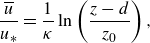 \begin{equation} \frac {\overline {u}}{u_*} = \frac {1}{\kappa } \ln \left (\frac {z-d}{z_0}\right ), \end{equation}
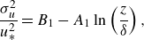 \begin{equation} \frac {{\sigma }_u^{2}}{u_{*}^{2}} = B_1-A_1 \ln \left (\frac {z}{\delta }\right ), \end{equation}
where $u$
is the streamwise velocity component,
$u$
is the streamwise velocity component, $z$
is the wall-normal distance with
$z$
is the wall-normal distance with $z=0$
set at the ground,
$z=0$
set at the ground, $d$
is the zero-plane displacement,
$d$
is the zero-plane displacement, $z_0$
is the momentum roughness length,
$z_0$
is the momentum roughness length, $\sigma _u^{2}=\overline {u^{\prime 2}}$
is the variance of
$\sigma _u^{2}=\overline {u^{\prime 2}}$
is the variance of $u$
, where the prime indicates turbulent fluctuations around the mean state, and the overline represents ensemble averaging (often represented by time averaging in the analysis of field data,
$u$
, where the prime indicates turbulent fluctuations around the mean state, and the overline represents ensemble averaging (often represented by time averaging in the analysis of field data, $u_*=(\tau /\rho )^{1/2}$
is the friction velocity, assumed to be the normalizing velocity for the flow statistics in the AEM, where
$u_*=(\tau /\rho )^{1/2}$
is the friction velocity, assumed to be the normalizing velocity for the flow statistics in the AEM, where $\tau$
is the wall (or ground) stress defined as
$\tau$
is the wall (or ground) stress defined as $\tau = \mu \left . ({\partial u}/{\partial z}) \right |_{z=0}$
,
$\tau = \mu \left . ({\partial u}/{\partial z}) \right |_{z=0}$
, $\mu$
is the dynamic viscosity of the fluid,
$\mu$
is the dynamic viscosity of the fluid, $\rho$
is the density of the fluid, and
$\rho$
is the density of the fluid, and $\delta$
is the outer length scale of the flow. The
$\delta$
is the outer length scale of the flow. The $\delta$
value is defined here as the ABL height, which differs from the ASL height or
$\delta$
value is defined here as the ABL height, which differs from the ASL height or $z$
used in previous work (Kunkel & Marusic Reference Kunkel and Marusic2006; Metzger et al. Reference Metzger, McKeon and Holmes2007; Marusic et al. 2013). These definitional differences translate to higher bulk Reynolds number here when compared to prior work. The coefficient
$z$
used in previous work (Kunkel & Marusic Reference Kunkel and Marusic2006; Metzger et al. Reference Metzger, McKeon and Holmes2007; Marusic et al. 2013). These definitional differences translate to higher bulk Reynolds number here when compared to prior work. The coefficient $\kappa$
is the von Kármán constant,
$\kappa$
is the von Kármán constant, $A_1$
is often referred to as the Townsend–Perry coefficient, and
$A_1$
is often referred to as the Townsend–Perry coefficient, and $B_1$
is an empirical coefficient dependent on the flow (i.e. pipe flow versus wind tunnels). Here,
$B_1$
is an empirical coefficient dependent on the flow (i.e. pipe flow versus wind tunnels). Here, $\kappa$
,
$\kappa$
, $A_1$
and
$A_1$
and $B_1$
are presumed to attain asymptotic constant values at very large Reynolds numbers defined as
$B_1$
are presumed to attain asymptotic constant values at very large Reynolds numbers defined as $Re_{\tau }=u_*\delta /\nu$
(Marusic et al. 2013; Smits et al. Reference Smits, McKeon and Marusic2011). For the vertical velocity (
$Re_{\tau }=u_*\delta /\nu$
(Marusic et al. 2013; Smits et al. Reference Smits, McKeon and Marusic2011). For the vertical velocity ( $w$
) variance (
$w$
) variance ( $\sigma _w^{2}=\overline {w}^{\prime 2}$
), the AEM predicts
$\sigma _w^{2}=\overline {w}^{\prime 2}$
), the AEM predicts
 \begin{equation} \frac {\sigma _w^{2}}{u_{*}^{2}}=B_2, \end{equation}
where $B_2$
is a coefficient that is also expected to reach an asymptotic constant value at very large
$B_2$
is a coefficient that is also expected to reach an asymptotic constant value at very large $Re_{\tau }$
. The logarithmic behaviour of
$Re_{\tau }$
. The logarithmic behaviour of $\overline {u}/u_*$
dates back to work before Townsend (e.g. Prandtl, von Kármán, Izakson and others, as reviewed elsewhere; see Monin & Yaglom Reference Monin and Yaglom1971), but this is consistent with Townsend’s attached-eddy hypothesis and thus is organized here as part of the AEM predictions.
$\overline {u}/u_*$
dates back to work before Townsend (e.g. Prandtl, von Kármán, Izakson and others, as reviewed elsewhere; see Monin & Yaglom Reference Monin and Yaglom1971), but this is consistent with Townsend’s attached-eddy hypothesis and thus is organized here as part of the AEM predictions.
The work here seeks to examine the applicability of the AEM to the adiabatic ASL with a focus on $\sigma _u^{2}$
, which is needed in a plethora of applications, such as footprint modelling and air quality studies (Banta et al. Reference Banta, Pichugina and Brewer2006; Wyngaard Reference Wyngaard, Venkatram and Wyngaard1988). Additionally, its numerical value is significant to wind energy assessments and to the stability of structures such as towers, bridges and trees (Lumley & Panofsky Reference Lumley and Panofsky1964). There is a growing number of laboratory studies supporting the logarithmic behaviour of
$\sigma _u^{2}$
, which is needed in a plethora of applications, such as footprint modelling and air quality studies (Banta et al. Reference Banta, Pichugina and Brewer2006; Wyngaard Reference Wyngaard, Venkatram and Wyngaard1988). Additionally, its numerical value is significant to wind energy assessments and to the stability of structures such as towers, bridges and trees (Lumley & Panofsky Reference Lumley and Panofsky1964). There is a growing number of laboratory studies supporting the logarithmic behaviour of $\sigma _u^{2}$
in the ISL (Marusic et al. Reference Marusic, McKeon, Monkewitz, Nagib, Smits and Sreenivasan2010, Reference Marusic, Monty, Hultmark and Smits2013). However, there have been few studies testing the logarithmic behaviour of
$\sigma _u^{2}$
in the ISL (Marusic et al. Reference Marusic, McKeon, Monkewitz, Nagib, Smits and Sreenivasan2010, Reference Marusic, Monty, Hultmark and Smits2013). However, there have been few studies testing the logarithmic behaviour of $\sigma _u^{2}$
and associated coefficients in the ASL, partly because profiling
$\sigma _u^{2}$
and associated coefficients in the ASL, partly because profiling $\sigma _u^{2}$
in the ASL demands high-fidelity measurements collected at multiple levels and obtaining such data is still challenging. Additionally, links between the logarithmic behaviour of
$\sigma _u^{2}$
in the ASL demands high-fidelity measurements collected at multiple levels and obtaining such data is still challenging. Additionally, links between the logarithmic behaviour of $\sigma _u^{2}$
and the ‘
$\sigma _u^{2}$
and the ‘ $-1$
’ scaling law in the streamwise velocity energy spectrum did not receive proper attention except in a handful of studies (e.g. Huang & Katul Reference Huang and Katul2022).
$-1$
’ scaling law in the streamwise velocity energy spectrum did not receive proper attention except in a handful of studies (e.g. Huang & Katul Reference Huang and Katul2022).
An extensive dataset with turbulence measurements at multiple levels within the ASL is used. These measurements enable a direct evaluation of the logarithmic behaviour of $\sigma _u^{2}$
in the near-neutral ASL, and the inference of
$\sigma _u^{2}$
in the near-neutral ASL, and the inference of $A_1$
from the profiles of
$A_1$
from the profiles of $\sigma _u^{2}$
. Before doing this, a brief review of current formulations of
$\sigma _u^{2}$
. Before doing this, a brief review of current formulations of $\sigma _u^{2}$
(or streamwise standard deviation
$\sigma _u^{2}$
(or streamwise standard deviation $\sigma _u$
) and the concomitant energy spectrum in turbulent boundary layers, in both atmosphere and laboratory settings, is provided.
$\sigma _u$
) and the concomitant energy spectrum in turbulent boundary layers, in both atmosphere and laboratory settings, is provided.
Table 1. A summary of formulations for the normalized streamwise velocity variance. Here, $\sigma _u$
represents the streamwise velocity standard deviation,
$\sigma _u$
represents the streamwise velocity standard deviation, $\sigma _u^{2}$
indicates the streamwise velocity variance,
$\sigma _u^{2}$
indicates the streamwise velocity variance, $z$
is the height of the sensor,
$z$
is the height of the sensor, $\delta$
is the boundary layer height,
$\delta$
is the boundary layer height, $L$
is the Obukhov length,
$L$
is the Obukhov length, $V_g$
is a viscous correction term that depends on the viscous Reynolds number
$V_g$
is a viscous correction term that depends on the viscous Reynolds number $Re^+ = z u_*/\nu$
, and
$Re^+ = z u_*/\nu$
, and $W_g$
is a wake correction term. The bulk Reynolds number is defined as
$W_g$
is a wake correction term. The bulk Reynolds number is defined as $Re_{\tau } = \delta u_*/\nu$
.
$Re_{\tau } = \delta u_*/\nu$
.
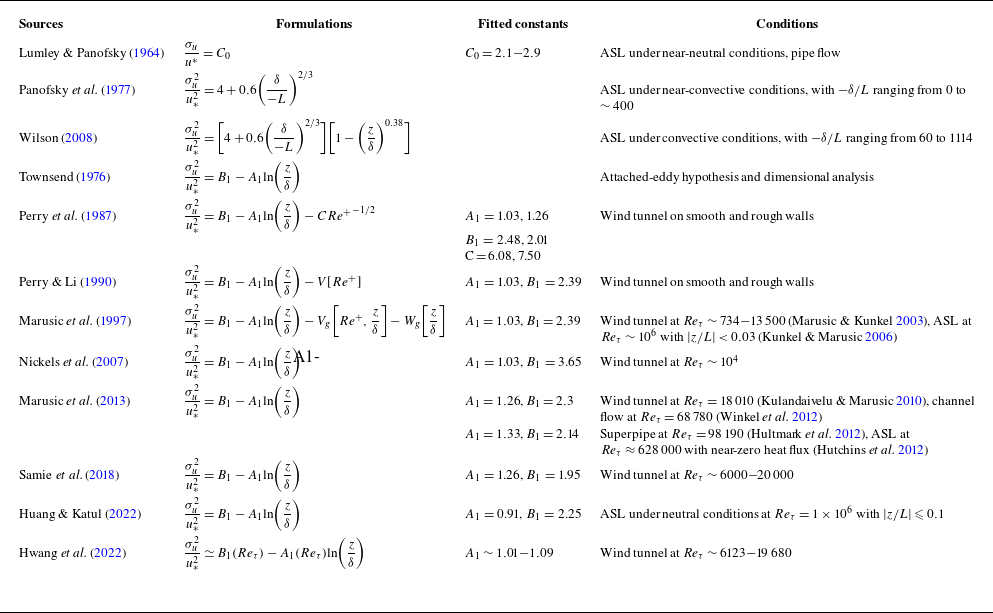
1.1. Magnitude of the turbulent velocity fluctuations
1.1.1. Review of ASL formulations for $\sigma _u$

Table 1 summarizes the formulations of $\sigma _u$
and
$\sigma _u$
and $\sigma _u^{2}$
found from field experiments in the ASL. According to Monin–Obukhov similarity theory (MOST), the streamwise velocity standard deviations can be expressed as (Obukhov Reference Obukhov1946; Monin & Obukhov Reference Monin and Obukhov1954)
$\sigma _u^{2}$
found from field experiments in the ASL. According to Monin–Obukhov similarity theory (MOST), the streamwise velocity standard deviations can be expressed as (Obukhov Reference Obukhov1946; Monin & Obukhov Reference Monin and Obukhov1954)
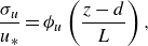 \begin{equation} \frac {\sigma _{u}}{u_*} = \phi _{u}\left (\frac {z-d}{L}\right ), \end{equation}
where $L$
is the Obukhov length measuring the height at which mechanical production of turbulence kinetic energy (TKE) approximately balances buoyancy production or destruction of TKE, whose calculation will be detailed in § 2.4. Here,
$L$
is the Obukhov length measuring the height at which mechanical production of turbulence kinetic energy (TKE) approximately balances buoyancy production or destruction of TKE, whose calculation will be detailed in § 2.4. Here, $\phi _{u}$
is a non-dimensional stability function that varies with the stability parameter
$\phi _{u}$
is a non-dimensional stability function that varies with the stability parameter $(z-d)/L$
. Under neutral conditions where
$(z-d)/L$
. Under neutral conditions where $|L|\rightarrow \infty$
,
$|L|\rightarrow \infty$
, $\phi _{u}$
reduces to
$\phi _{u}$
reduces to
 \begin{equation} \frac {\sigma _u}{u_*} = C_0. \end{equation}
Many ASL measurements conducted under near-neutral conditions as well as laboratory flows have been used to fit the empirical parameter $C_0$
. Lumley & Panofsky (Reference Lumley and Panofsky1964) surveyed several experiments, and stated that
$C_0$
. Lumley & Panofsky (Reference Lumley and Panofsky1964) surveyed several experiments, and stated that $C_0$
appears to be independent of
$C_0$
appears to be independent of $z$
but varies with terrain, with values ranging between 2.1 and 2.9. The survey also noted that under varying stability conditions, vertical and horizontal velocity components exhibit distinct behaviours. While the vertical velocity standard deviation aligns well with MOST predictions, streamwise velocity components are affected differently by
$z$
but varies with terrain, with values ranging between 2.1 and 2.9. The survey also noted that under varying stability conditions, vertical and horizontal velocity components exhibit distinct behaviours. While the vertical velocity standard deviation aligns well with MOST predictions, streamwise velocity components are affected differently by $z-d$
and
$z-d$
and $1/L$
. Specifically, a change in
$1/L$
. Specifically, a change in $z$
has a negligible effect on streamwise velocity standard deviations, whereas a change in stability (e.g.
$z$
has a negligible effect on streamwise velocity standard deviations, whereas a change in stability (e.g. $z/L$
) has a pronounced effect. A recent study attributed this limitation of MOST to the anisotropy of the Reynolds stress tensor (Stiperski & Calaf Reference Stiperski and Calaf2023).
$z/L$
) has a pronounced effect. A recent study attributed this limitation of MOST to the anisotropy of the Reynolds stress tensor (Stiperski & Calaf Reference Stiperski and Calaf2023).
To account for the ‘non-MOST’ behaviour of streamwise velocity components and the increase of streamwise wind fluctuations with the deepening of boundary layer height under near-convective conditions, Panofsky et al. (Reference Panofsky, Tennekes, Lenschow and Wyngaard1977) proposed an empirical formulation fitted by ASL observations from 30 m to 87 m, with $-\delta /L$
ranging from 0 to
$-\delta /L$
ranging from 0 to $\sim 400$
given by
$\sim 400$
given by
 \begin{equation} \frac {\sigma _u^{2}}{u_{*}^{2}} = 4 + 0.6 \left (\frac {\delta }{-L} \right )^{2/3}. \end{equation}
It should be noted that under neutral conditions, (1.6) is similar to (1.5). This formulation became popular in atmospheric sciences (Wyngaard Reference Wyngaard, Venkatram and Wyngaard1988), although it assumed that changes in $z$
have a negligible effect on
$z$
have a negligible effect on $\sigma _u$
even for near-neutral conditions. Another extensive study was undertaken for unstable conditions with
$\sigma _u$
even for near-neutral conditions. Another extensive study was undertaken for unstable conditions with $-\delta /L$
ranging from 60 to 1114 (Wilson Reference Wilson2008) where TKE production and TKE dissipation rates were in approximate balance. These experiments reported a mild
$-\delta /L$
ranging from 60 to 1114 (Wilson Reference Wilson2008) where TKE production and TKE dissipation rates were in approximate balance. These experiments reported a mild $z$
-dependence of the streamwise velocity variance. A refinement to Panofsky’s formulation followed, given as
$z$
-dependence of the streamwise velocity variance. A refinement to Panofsky’s formulation followed, given as
 \begin{equation} \frac {\sigma _u^{2}}{u_{*}^{2}} = \left [4+0.6\left (\frac {\delta }{-L}\right )^{2/3}\right ]\left [1-\left (\frac {z}{\delta }\right )^{0.38}\right ]. \end{equation}
In the near-neutral limit, this expression is reduced to
 \begin{equation} \frac {\sigma _u^{2}}{u_{*}^{2}} = 4\left [1-\left (\frac {z}{\delta }\right )^{0.38}\right ], \end{equation}
which confirms that increasing $z/\delta$
reduces
$z/\delta$
reduces $\sigma _u^{2}/u_*^{2}$
, as expected from the AEM. Moreover, for very small
$\sigma _u^{2}/u_*^{2}$
, as expected from the AEM. Moreover, for very small $z/\delta$
, the predicted
$z/\delta$
, the predicted $\sigma _u/u_*=2$
agrees with the expected values reported for the ASL (Lumley & Panofsky Reference Lumley and Panofsky1964).
$\sigma _u/u_*=2$
agrees with the expected values reported for the ASL (Lumley & Panofsky Reference Lumley and Panofsky1964).
Nonetheless, those developments have been viewed as ‘adjustments’ to MOST, and have made no apparent contact with the AEM. In fact, after the work of Kaimal (Reference Kaimal1978), Bradshaw (Reference Bradshaw1978) commented that MOST formulations for the ASL appear to have missed predictions from the AEM about the role of $\delta$
in
$\delta$
in $\sigma _u^{2}/u_*^{2}$
(Bradshaw Reference Bradshaw1967), which is briefly reviewed next.
$\sigma _u^{2}/u_*^{2}$
(Bradshaw Reference Bradshaw1967), which is briefly reviewed next.
1.1.2. Townsend’s attached-eddy hypothesis
The AEM postulates that turbulence in wall-bounded flows can be described by a hierarchy of self-similar eddies attached to the wall (Townsend Reference Townsend1976). These eddies are geometrically similar at different scales, with their size proportional to their distance from the wall. Using the equilibrium layer hypothesis where the mechanical production of TKE balances the viscous dissipation, the AEM predicts a specific scaling law in the energy spectrum (Perry et al. Reference Perry, Henbest and Chong1986; Perry & Li Reference Perry and Li1990). Further, by integrating the streamwise velocity spectrum across all wavenumbers, $\sigma _u^{2}$
can be formulated as in (1.2) for the overlap region (where the inner region overlaps with the outer region) of turbulent flows. This relation is a cornerstone of the AEM, linking the spectral characteristics of turbulence at a given
$\sigma _u^{2}$
can be formulated as in (1.2) for the overlap region (where the inner region overlaps with the outer region) of turbulent flows. This relation is a cornerstone of the AEM, linking the spectral characteristics of turbulence at a given $z$
to the profile of
$z$
to the profile of $\sigma _u^{2}$
(Townsend Reference Townsend1976; Perry & Chong Reference Perry and Chong1982). Meanwhile, the only difference between the smooth and rough walls from the point of view of the Perry & Chong (Reference Perry and Chong1982) model is that the smallest hierarchy scales with
$\sigma _u^{2}$
(Townsend Reference Townsend1976; Perry & Chong Reference Perry and Chong1982). Meanwhile, the only difference between the smooth and rough walls from the point of view of the Perry & Chong (Reference Perry and Chong1982) model is that the smallest hierarchy scales with $\nu /u_*$
on smooth walls, while it scales with the roughness length on rough walls.
$\nu /u_*$
on smooth walls, while it scales with the roughness length on rough walls.
Since the classic book by Townsend (Reference Townsend1976), the AEM has drawn significant experimental and theoretical interest (see table 1). Perry et al. (Reference Perry, Henbest and Chong1986) expanded the AEM to include near-wall regions, addressing inner flow dynamics, and providing a theoretical and experimental foundation for the logarithmic law. Subsequently, Perry et al. (Reference Perry, Lim and Henbest1987) introduced a $C\, {Re^+}^{-1/2}$
term that depends on the viscous Reynolds number (
$C\, {Re^+}^{-1/2}$
term that depends on the viscous Reynolds number ( $Re^+ = z u_*/\nu$
) to (1.2) to account for different surface types – smooth, rough and wavy – identifying distinct coefficients (
$Re^+ = z u_*/\nu$
) to (1.2) to account for different surface types – smooth, rough and wavy – identifying distinct coefficients ( $A_1$
,
$A_1$
, $B_1$
,
$B_1$
, $C$
) for each. In a further advancement, Perry & Li (Reference Perry and Li1990) incorporated a viscous correction term
$C$
) for each. In a further advancement, Perry & Li (Reference Perry and Li1990) incorporated a viscous correction term $V[Re^+]$
, arguing for the formulation’s independence from Reynolds number variations, and showing that the constant
$V[Re^+]$
, arguing for the formulation’s independence from Reynolds number variations, and showing that the constant $A_1$
is the same on both the smooth and rough walls. Building on these foundations, Marusic et al. (Reference Marusic, Uddin and Perry1997) proposed a similarity relation to describe the streamwise velocity variance in the logarithmic region, considering inviscid attached eddies and incorporating a viscous correction term
$A_1$
is the same on both the smooth and rough walls. Building on these foundations, Marusic et al. (Reference Marusic, Uddin and Perry1997) proposed a similarity relation to describe the streamwise velocity variance in the logarithmic region, considering inviscid attached eddies and incorporating a viscous correction term $V_g[Re^+, {z}/{\delta }]$
in the inner region, and a wake correction term
$V_g[Re^+, {z}/{\delta }]$
in the inner region, and a wake correction term $W_g[ {z}/{\delta }]$
in the outer region. This formulation was evaluated using wind tunnel and near-neutral ASL data with success.
$W_g[ {z}/{\delta }]$
in the outer region. This formulation was evaluated using wind tunnel and near-neutral ASL data with success.
Metzger et al. (Reference Metzger, McKeon and Holmes2007) tested this similarity formulation using data collected at the Surface Layer Turbulence and Environmental Science Test (SLTEST) facility, confirming the logarithmic behaviour of $\sigma _u^{2}$
in near-neutral ASL conditions. Nickels et al. (Reference Nickels, Marusic, Hafez, Hutchins and Chong2007) further explored this formulation by neglecting the correction terms for the viscous and outer flow effects, which were deemed insignificant in their study. These experiments matched well with AEM predictions when setting
$\sigma _u^{2}$
in near-neutral ASL conditions. Nickels et al. (Reference Nickels, Marusic, Hafez, Hutchins and Chong2007) further explored this formulation by neglecting the correction terms for the viscous and outer flow effects, which were deemed insignificant in their study. These experiments matched well with AEM predictions when setting $A_1 = 1.03$
, consistent with the prior value reported in Perry & Li (Reference Perry and Li1990).
$A_1 = 1.03$
, consistent with the prior value reported in Perry & Li (Reference Perry and Li1990).
Further experimental support for (1.2) was provided by Marusic et al. (Reference Marusic, Monty, Hultmark and Smits2013), who analyzed four datasets including boundary layers, pipe flow and ASL measurements with $2\times 10^4 \lt Re_{\tau } \lt 6\times 10^5$
. Specifically, neutral boundary layer conditions were identified by near-zero heat flux in the ASL dataset (Hutchins et al. Reference Hutchins, Chauhan, Marusic, Monty and Klewicki2012). Their results not only affirmed the presence of a universal logarithmic region, but also estimated
$2\times 10^4 \lt Re_{\tau } \lt 6\times 10^5$
. Specifically, neutral boundary layer conditions were identified by near-zero heat flux in the ASL dataset (Hutchins et al. Reference Hutchins, Chauhan, Marusic, Monty and Klewicki2012). Their results not only affirmed the presence of a universal logarithmic region, but also estimated $A_1$
to be approximately 1.26 for lab flow and 1.33 for ASL data, which is different from the previous estimation
$A_1$
to be approximately 1.26 for lab flow and 1.33 for ASL data, which is different from the previous estimation $A_1= 1.03$
. They also acknowledged the uncertainties in
$A_1= 1.03$
. They also acknowledged the uncertainties in $A_1$
estimation arising from the curve-fitting procedure (e.g.
$A_1$
estimation arising from the curve-fitting procedure (e.g. $\pm 0.17$
in their ASL dataset). Samie et al. (Reference Samie, Marusic, Hutchins, Fu, Fan, Hultmark and Smits2018) reported
$\pm 0.17$
in their ASL dataset). Samie et al. (Reference Samie, Marusic, Hutchins, Fu, Fan, Hultmark and Smits2018) reported $A_1 = 1.26$
based on wind tunnel data within the range
$A_1 = 1.26$
based on wind tunnel data within the range $6000 \lt Re_{\tau } \lt 20000$
. Similarly, Wang & Zheng (Reference Wang and Zheng2016) found that their ASL experiments supported the estimate
$6000 \lt Re_{\tau } \lt 20000$
. Similarly, Wang & Zheng (Reference Wang and Zheng2016) found that their ASL experiments supported the estimate $A_1 = 1.33$
, while Huang & Katul (Reference Huang and Katul2022) used SLTEST data near the wall (just above the roughness layer) to study the high-order moments of the streamwise velocity, finding a fitted
$A_1 = 1.33$
, while Huang & Katul (Reference Huang and Katul2022) used SLTEST data near the wall (just above the roughness layer) to study the high-order moments of the streamwise velocity, finding a fitted $A_1$
of approximately 0.9 under near-neutral conditions (
$A_1$
of approximately 0.9 under near-neutral conditions ( $| z/L| \leqslant 0.1$
). This value appears to be closer to the value reported by Katul & Chu (Reference Katul and Chu1998) for the near-neutral ASL derived from streamwise velocity spectra.
$| z/L| \leqslant 0.1$
). This value appears to be closer to the value reported by Katul & Chu (Reference Katul and Chu1998) for the near-neutral ASL derived from streamwise velocity spectra.
Alongside the variability in $A_1$
, the debate continues regarding the origin of the log law of the streamwise velocity variance. Some studies have employed spectral budget analysis and dimensional analysis, complemented by laboratory experiments (Nikora Reference Nikora1999; Banerjee & Katul Reference Banerjee and Katul2013), to explain the logarithmic behaviour of streamwise velocity variance. Recently, Hwang et al. (Reference Hwang, Hutchins and Marusic2022) introduced a model inspired by Townsend’s original work, addressing the spectrum in the logarithmic layer for various
$A_1$
, the debate continues regarding the origin of the log law of the streamwise velocity variance. Some studies have employed spectral budget analysis and dimensional analysis, complemented by laboratory experiments (Nikora Reference Nikora1999; Banerjee & Katul Reference Banerjee and Katul2013), to explain the logarithmic behaviour of streamwise velocity variance. Recently, Hwang et al. (Reference Hwang, Hutchins and Marusic2022) introduced a model inspired by Townsend’s original work, addressing the spectrum in the logarithmic layer for various $z/\delta$
values. This model suggests that the coefficients
$z/\delta$
values. This model suggests that the coefficients $A_1$
and
$A_1$
and $B_1$
depend on the Reynolds number. Their analysis of wind tunnel data at
$B_1$
depend on the Reynolds number. Their analysis of wind tunnel data at $Re_{\tau } \sim 6123 {-}19\,680$
indicated that the approximated
$Re_{\tau } \sim 6123 {-}19\,680$
indicated that the approximated $A_1$
values vary between 1.01 and 1.09. Furthermore, their model challenges the notion that a ‘
$A_1$
values vary between 1.01 and 1.09. Furthermore, their model challenges the notion that a ‘ $-1$
’ power law in the streamwise energy spectrum is necessary for the logarithmic behaviour in streamwise velocity variance. This evolving understanding underscores the need to verify the universality of the logarithmic behaviour of streamwise velocity variance, particularly within the ASL, and assess to what extent the coefficient
$-1$
’ power law in the streamwise energy spectrum is necessary for the logarithmic behaviour in streamwise velocity variance. This evolving understanding underscores the need to verify the universality of the logarithmic behaviour of streamwise velocity variance, particularly within the ASL, and assess to what extent the coefficient $A_1$
can be derived from the spectrum of the streamwise velocity at a single level
$A_1$
can be derived from the spectrum of the streamwise velocity at a single level $z$
.
$z$
.
1.2. Streamwise velocity energy spectrum
In the production range, TKE is generated primarily by the mean shear and ‘active’ eddies. The streamwise velocity energy spectrum $E_{uu}(k)$
as a function of streamwise wavenumber
$E_{uu}(k)$
as a function of streamwise wavenumber $k$
in this range typically exhibits a peak corresponding to the energy-containing eddies. In the absence of long-term trends in the record,
$k$
in this range typically exhibits a peak corresponding to the energy-containing eddies. In the absence of long-term trends in the record, $ E_{uu}(k)$
is expected to level off to a constant value as
$ E_{uu}(k)$
is expected to level off to a constant value as $k\rightarrow 0$
(Kaimal & Finnigan Reference Kaimal and Finnigan1994). The AEM argues that in the limit
$k\rightarrow 0$
(Kaimal & Finnigan Reference Kaimal and Finnigan1994). The AEM argues that in the limit $Re_{\tau } \rightarrow \infty$
, and when the wall-normal distance is much smaller than the boundary layer height (
$Re_{\tau } \rightarrow \infty$
, and when the wall-normal distance is much smaller than the boundary layer height ( $z \ll \delta$
), the pre-multiplied power spectral density for
$z \ll \delta$
), the pre-multiplied power spectral density for $k \sim \mathcal{O}(1/\delta )$
should exhibit a characteristic
$k \sim \mathcal{O}(1/\delta )$
should exhibit a characteristic $\delta$
scaling:
$\delta$
scaling:
 \begin{equation} \frac {k\, E_{uu}(k,z)}{u_{*}^{2}} = h_1(k\delta ). \end{equation}
Similarly, for $k \sim \mathcal{O}(1/z)$
, the pre-multiplied power spectral density should follow a
$k \sim \mathcal{O}(1/z)$
, the pre-multiplied power spectral density should follow a $z$
scaling:
$z$
scaling:
 \begin{equation} \frac {k\,E_{uu}(k,z)}{u_{*}^{2}} = h_2(kz).\end{equation}
In the overlap region where both the outer scaling ( $\delta$
) and the inner scaling (
$\delta$
) and the inner scaling ( $z$
) are valid simultaneously (
$z$
) are valid simultaneously ( $1/\delta \ll k \ll 1/z$
), matching these scaling arguments requires
$1/\delta \ll k \ll 1/z$
), matching these scaling arguments requires
 \begin{equation} h_1(k\delta ) = h_2(kz) = C_1, \end{equation}
where $h_1$
and
$h_1$
and $h_2$
are two universal functions, and
$h_2$
are two universal functions, and $C_1$
is a constant independent of both
$C_1$
is a constant independent of both $k z$
and
$k z$
and $k \delta$
, corresponding to coefficient
$k \delta$
, corresponding to coefficient $A_1$
in (1.2).
$A_1$
in (1.2).
This matching also suggests that in the overlap region (or ISL), the power spectral density must satisfy
 \begin{equation} E_{uu}(k)=C_1 u_{*}^{2} k^{-1}, \end{equation}
and is independent of $z$
and
$z$
and $\delta$
. This spectrum is consistent with the presence of large, energy-containing, self-similar eddies attached to the wall (Bradshaw Reference Bradshaw1967; Perry & Abell Reference Perry and Abell1977). The
$\delta$
. This spectrum is consistent with the presence of large, energy-containing, self-similar eddies attached to the wall (Bradshaw Reference Bradshaw1967; Perry & Abell Reference Perry and Abell1977). The $k^{-1}$
power law, originally reported in pipes (Klebanoff Reference Klebanoff1954), has also been confirmed in many pipe flow experiments since then (Bremhorst & Bullock Reference Bremhorst and Bullock1970; Perry & Abell Reference Perry and Abell1975, Reference Perry and Abell1977; Bullock et al. Reference Bullock, Cooper and Abernathy1978).
$k^{-1}$
power law, originally reported in pipes (Klebanoff Reference Klebanoff1954), has also been confirmed in many pipe flow experiments since then (Bremhorst & Bullock Reference Bremhorst and Bullock1970; Perry & Abell Reference Perry and Abell1975, Reference Perry and Abell1977; Bullock et al. Reference Bullock, Cooper and Abernathy1978).
However, observing a clear $k^{-1}$
scaling in
$k^{-1}$
scaling in $E_{uu}(k,z)$
is not straightforward. It was already pointed out by Antonia & Raupach (Reference Antonia and Raupach1993) that while the
$E_{uu}(k,z)$
is not straightforward. It was already pointed out by Antonia & Raupach (Reference Antonia and Raupach1993) that while the $k^{-1}$
scaling in
$k^{-1}$
scaling in $E_{uu}(k,z)$
was observed in their high Reynolds number wind tunnel experiments, they precluded its existence in the ASL, citing unavoidable ground (and thermal) inhomogeneity and weak non-stationarity. It was also suggested that the logarithmic layer could be influenced by large-scale motion induced by non-turbulence processes (Wang & Zheng Reference Wang and Zheng2016). The presence of other turbulence structures, such as detached eddies, wake turbulence or other flow irregularities, can contribute to the energy spectrum and obscure the
$E_{uu}(k,z)$
was observed in their high Reynolds number wind tunnel experiments, they precluded its existence in the ASL, citing unavoidable ground (and thermal) inhomogeneity and weak non-stationarity. It was also suggested that the logarithmic layer could be influenced by large-scale motion induced by non-turbulence processes (Wang & Zheng Reference Wang and Zheng2016). The presence of other turbulence structures, such as detached eddies, wake turbulence or other flow irregularities, can contribute to the energy spectrum and obscure the $k^{-1}$
behaviour (Baars & Marusic Reference Baars and Marusic2020) that would otherwise be observed in the production range (i.e. the range over which TKE is produced) dominated by attached eddies.
$k^{-1}$
behaviour (Baars & Marusic Reference Baars and Marusic2020) that would otherwise be observed in the production range (i.e. the range over which TKE is produced) dominated by attached eddies.
Despite these complexities, several experiments reported a $k^{-1}$
power law in the ASL, with
$k^{-1}$
power law in the ASL, with $C_1$
values ranging from 0.9 to 1.1, as summarized in table 2. Compared to the values in table 1,
$C_1$
values ranging from 0.9 to 1.1, as summarized in table 2. Compared to the values in table 1, $C_1$
determined from fitting
$C_1$
determined from fitting ${k\,E_{uu}(k,z)}/{u_{*}^{2}}$
tends to be lower than
${k\,E_{uu}(k,z)}/{u_{*}^{2}}$
tends to be lower than $A_1$
derived from fitting the profile of
$A_1$
derived from fitting the profile of $\sigma _u^{2}$
. This discrepancy may be attributed to uncertainties in the fitting process and potential misalignment between the
$\sigma _u^{2}$
. This discrepancy may be attributed to uncertainties in the fitting process and potential misalignment between the $x$
-axis and the incoming wind. Such misalignment could introduce biases from the cross-stream component, thereby reducing the effective production measured (Huang & Katul Reference Huang and Katul2022). However, no study has yet simultaneously obtained and compared both
$x$
-axis and the incoming wind. Such misalignment could introduce biases from the cross-stream component, thereby reducing the effective production measured (Huang & Katul Reference Huang and Katul2022). However, no study has yet simultaneously obtained and compared both $A_1$
and
$A_1$
and $C_1$
from the same ASL experiments (i.e. very high Reynolds number), which partly motivated the study here.
$C_1$
from the same ASL experiments (i.e. very high Reynolds number), which partly motivated the study here.
Table 2. A summary of experiments reporting a $k^{-1}$
scaling in the ISL, along with the corresponding
$k^{-1}$
scaling in the ISL, along with the corresponding $C_1$
values.
$C_1$
values.
1.3. Objectives
The logarithmic behaviours of the streamwise velocity variance and the $k^{-1}$
scaling in the energy spectra of streamwise velocity in the ASL, as well as their interconnection, are to be explored. Specifically, the following questions are to be addressed.
$k^{-1}$
scaling in the energy spectra of streamwise velocity in the ASL, as well as their interconnection, are to be explored. Specifically, the following questions are to be addressed.
-
(i) Can a logarithmic profile of streamwise velocity variance be observed over a flat, homogeneous surface in the adiabatic ASL?
-
(ii) Using these ASL measurements, what are the dominant factors that influence the variability in
$A_1$
? -
(iii) Does a
$k^{-1}$
scaling regime exist in the energy spectrum of the streamwise velocity in the adiabatic ASL with a plateau value
$C_1=A_1$
?


To answer these questions, the paper is organized as follows. Section 2 introduces the field experiment and outlines the data processing and screening methods. Section 3 presents and discusses the results. Section 4 concludes and offers an outlook.
Figure 1. (a) Topography of the ESRP, Idaho, USA, based on the 30 m resolution Shuttle Radar Topography Mission (SRTM) dataset (Farr et al. Reference Farr2007). The red star marks the location of the 62 m tower GRID3. (b) A photo of the 62 m tower, viewing from the south-east. (c) The configuration of the 62 m and 10 m towers. (d) Dominant land surface vegetation at the site.
2. Methods
2.1. Study site
The study area is located in the Eastern Snake River Plain (ESRP), extending from Twin Falls, Idaho, to the Yellowstone Plateau in the north-east (see figure 1 a). The ESRP generally runs in a north-east to south-west direction, and is bordered by large mountain ranges. To the northwest are the Lost River, Lemhi and Bitterroot mountain ranges, which are oriented perpendicularly in a north-west to south-east direction, and rise to approximately 3000 m above mean sea level, approximately 1800 m above the mean elevation of the ESRP. Across the ESRP, the elevation is higher to the north and north-east, and lower to the south and south-west (Clawson et al. Reference Clawson, Rich, Eckman, Hukari, Finn and Reese2018). This area is commonly influenced by general ESRP downslope winds from the north-east during the night. During the day, this area often experiences synoptic south-westerly winds, and frequent afternoon winds from the south-west that are driven by radiative heating. Under these two prevailing wind conditions, the site has a relatively flat and uniform fetch extending tens of kilometres upwind (Finn et al. Reference Finn, Carter, Eckman, Rich, Gao and Liu2018a ,Reference Finn, Eckman, Gao and Liu b ). Additionally, the area experiences shallow nocturnal down-valley winds from the north-west associated with the Big Lost River channel.
2.2. Field experiments
The experiment took place at the Idaho National Laboratory (INL) facility (43 $^\circ 35^{\prime}30^{\prime\prime}$
N, 112
$^\circ 35^{\prime}30^{\prime\prime}$
N, 112 $^\circ 55^{\prime}50^{\prime\prime}$
W). The general surface of the INL, like that of the entire ESRP, consists of rolling grasslands and sagebrush (see figure 1
d). Previous work reported that this site is characterized by a zero-plane displacement (
$^\circ 55^{\prime}50^{\prime\prime}$
W). The general surface of the INL, like that of the entire ESRP, consists of rolling grasslands and sagebrush (see figure 1
d). Previous work reported that this site is characterized by a zero-plane displacement ( $d$
) close to zero, and median
$d$
) close to zero, and median $z_0$
approximately 3 cm for south-west winds and 3.8 cm for north-east winds (Finn et al. Reference Finn, Clawson, Eckman, Liu, Russell, Gao and Brooks2016; Clawson et al. Reference Clawson, Rich, Eckman, Hukari, Finn and Reese2018). As will be seen later, our estimates of
$z_0$
approximately 3 cm for south-west winds and 3.8 cm for north-east winds (Finn et al. Reference Finn, Clawson, Eckman, Liu, Russell, Gao and Brooks2016; Clawson et al. Reference Clawson, Rich, Eckman, Hukari, Finn and Reese2018). As will be seen later, our estimates of $ z_0$
have a median value of 8 cm during the study period, which extended from 20 September 2020 to 22 April 2021. In this period, 12 measurement levels of eddy-covariance systems were deployed on two towers. The primary measurement site consisted of a 62 m meteorological tower (GRID3) instrumented at eight levels (9, 12.5, 16.5, 23, 30, 40, 50 and 60 m). Additionally, an auxiliary 10 m tower instrumented at four levels (1.2, 2, 3.5 and 6 m) (see figure 1
b,c) was located approximately 15 m away from the GRID3 tower, and the alignment of the two towers was roughly perpendicular to the predominant mean wind direction. Despite the relatively flat and homogeneous surface, this set-up resulted in different measurement footprints between the two towers. The 62 m tower was equipped with retractable square booms (Tower Systems, Inc.) measuring 3.6 m (12 ft), mounted horizontally to provide stable platforms for the sensors. On the 10 m tower, 1.8 m (6 ft) poles were used, ensuring that the sensors were placed approximately 1.5 m away from the tower’s structure.
$ z_0$
have a median value of 8 cm during the study period, which extended from 20 September 2020 to 22 April 2021. In this period, 12 measurement levels of eddy-covariance systems were deployed on two towers. The primary measurement site consisted of a 62 m meteorological tower (GRID3) instrumented at eight levels (9, 12.5, 16.5, 23, 30, 40, 50 and 60 m). Additionally, an auxiliary 10 m tower instrumented at four levels (1.2, 2, 3.5 and 6 m) (see figure 1
b,c) was located approximately 15 m away from the GRID3 tower, and the alignment of the two towers was roughly perpendicular to the predominant mean wind direction. Despite the relatively flat and homogeneous surface, this set-up resulted in different measurement footprints between the two towers. The 62 m tower was equipped with retractable square booms (Tower Systems, Inc.) measuring 3.6 m (12 ft), mounted horizontally to provide stable platforms for the sensors. On the 10 m tower, 1.8 m (6 ft) poles were used, ensuring that the sensors were placed approximately 1.5 m away from the tower’s structure.
The eddy-covariance systems used in the experiment included two models of triaxial sonic anemometers (CSAT3B and CSAT3, Campbell Scientific, Inc.), and two models of infrared gas analysers (IRGAs; LI7500RS and LI7500, LICOR, Inc.). The sonic anemometers measured the velocity components along the north–south, east–west and vertical directions, respectively, relative to the reference frame fixed to the sonic anemometer. Sonic azimuth was estimated by comparing the calculated and measured wind directions from sonics and wind vanes. The sonic anemometers were oriented slightly towards the north-north-west, rather than directly north. The IRGAs measured the densities of water vapour and $\mathrm{CO_2}$
. The sampling frequency was 10 Hz for all anemometers. The CSAT3s had vertical sonic paths of 10 cm and horizontal paths of 5.8 cm, operating in a pulsed acoustic mode. Corrections for the effects of humidity and density fluctuations on the turbulent fluctuations of sonic temperature and the densities of water vapour and
$\mathrm{CO_2}$
. The sampling frequency was 10 Hz for all anemometers. The CSAT3s had vertical sonic paths of 10 cm and horizontal paths of 5.8 cm, operating in a pulsed acoustic mode. Corrections for the effects of humidity and density fluctuations on the turbulent fluctuations of sonic temperature and the densities of water vapour and $\mathrm{CO_2}$
have been detailed elsewhere (Gao et al. Reference Gao, Liu, Li, Yang, Walden, Li and Bogoev2024). These scalar measurements are needed only to estimate whether
$\mathrm{CO_2}$
have been detailed elsewhere (Gao et al. Reference Gao, Liu, Li, Yang, Walden, Li and Bogoev2024). These scalar measurements are needed only to estimate whether $L$
is sufficiently large and thus whether the flow is near neutral.
$L$
is sufficiently large and thus whether the flow is near neutral.
2.3. Data processing
Data processing involves coordinate rotation, detrending and neutral case screening. High-frequency spectral corrections are neglected because the contribution from the high-frequency region to turbulence intensity is small. For example, the data indicate that the errors caused by path averaging are 2–3 orders of magnitude smaller than the streamwise velocity variance ( ${\sigma }_u^{2}$
).
${\sigma }_u^{2}$
).
2.3.1. Averaging period
In the analysis of ASL data, fluctuations with periods less than approximately one hour are generally considered turbulence, while slower fluctuations are synoptic-scale and treated as part of the mean flow (Wyngaard Reference Wyngaard1992). Consequently, a one-hour averaging period is selected as a compromise between the need to resolve large eddies reliably and stationarity considerations. However, Metzger et al. (Reference Metzger, McKeon and Holmes2007) suggested that the neutral periods are often short, of the order of several minutes. Previous studies have used various averaging periods depending on the stability and conditions of the boundary layer. For instance, 10 min was used in the stable boundary layer in the CASES-99 experiment (Banta et al. Reference Banta, Pichugina and Brewer2006), 30 min in the unstable conditions when mechanical production of TKE was compared to viscous dissipation (Wilson Reference Wilson2008), 20 min in neutral conditions in the SLTEST experiment (Metzger et al. Reference Metzger, McKeon and Holmes2007), and 1 hour in neutral conditions in the same SLTEST experiment (Hutchins et al. Reference Hutchins, Chauhan, Marusic, Monty and Klewicki2012). Additionally, 30 min was used in SLTEST (Huang & Katul Reference Huang and Katul2022), 15 min in the unstable LATEX experiment (Li & Bou-Zeid Reference Li and Bou-Zeid2011), and 1 min for stable and 30 min for unstable conditions across 13 datasets (Stiperski & Calaf Reference Stiperski and Calaf2023).
A shorter sampling period, while increasing steadiness in mean meteorological conditions, can also affect statistical convergence by reducing sample size, increasing sensitivity to outliers, and potentially biasing the representative nature of the data. In general, the difference between ensemble averaging (the sought quantity) and time averaging is labelled as systematic bias. This bias declines with reduced $2 T_L/T_p$
(Lenschow et al. Reference Lenschow, Mann and Kristensen1994), where
$2 T_L/T_p$
(Lenschow et al. Reference Lenschow, Mann and Kristensen1994), where $T_L$
is the integral time scale of a flow variable, and
$T_L$
is the integral time scale of a flow variable, and $T_p$
is the averaging period. Typical
$T_p$
is the averaging period. Typical $T_L$
values for the streamwise velocity are of the order of 1–2 min, hence selecting
$T_L$
values for the streamwise velocity are of the order of 1–2 min, hence selecting $T_p=60$
min is acceptable for reducing the systematic bias.
$T_p=60$
min is acceptable for reducing the systematic bias.
A comparison between 1 hour and 30 min averaging periods is also conducted to assess the sensitivity of the results to the choice of averaging window. The results suggest that the 30 min averaging period only increases the variability in the fitted coefficients, while the overall conclusions of this study remain unaltered. Therefore, the 1 hour averaging period is considered a more suitable choice for the analysis, striking a balance between reducing systematic bias and maintaining statistical robustness.
2.3.2. Coordinate rotation
Assuming that the sonic anemometers are nearly level, requiring only minor tilt corrections to align the vertical axis perpendicular to the mean flow, the double rotation method (Wilczak et al. Reference Wilczak, Oncley and Stage2001) involves two sequential rotations: first, a pitch rotation to set the mean vertical velocity component ( $\overline {w}$
) to zero; and second, a yaw rotation to set the mean lateral velocity component (
$\overline {w}$
) to zero; and second, a yaw rotation to set the mean lateral velocity component ( $\overline {v}$
) to zero. Given the relatively flat and homogeneous terrain, this standard method is initially applied to correct the tilt of the anemometers.
$\overline {v}$
) to zero. Given the relatively flat and homogeneous terrain, this standard method is initially applied to correct the tilt of the anemometers.
Another commonly used rotation procedure in micrometeorology is the planar fit method (Wilczak et al. Reference Wilczak, Oncley and Stage2001; Aubinet et al. Reference Aubinet, Vesala and Papale2012), which is particularly suited for complex terrain where a non-zero mean vertical velocity may exist. To evaluate whether the fitted coefficients in the AEM are sensitive to different coordinate rotation methods, this study applies the planar fit method. The data are first grouped into six wind direction sectors at 60 $^\circ$
intervals, then a plane is fitted to all the data within each sector over the entire seven-month experimental period.
$^\circ$
intervals, then a plane is fitted to all the data within each sector over the entire seven-month experimental period.
2.3.3. Detrending
After the coordinate rotation, the time series in figure 2(a) shows a superposition of the high-frequency turbulent fluctuations and low-frequency oscillations. Detrending is employed to remove long-term trends or patterns in the data, which can result from various factors, such as instrument drift and atmospheric changes (Moncrieff et al. Reference Moncrieff, Clement, Finnigan and Meyers2004). By removing the low-frequency content, the analysis can focus on short-term variability (i.e. turbulence) and ensure a certain amount of stationarity.
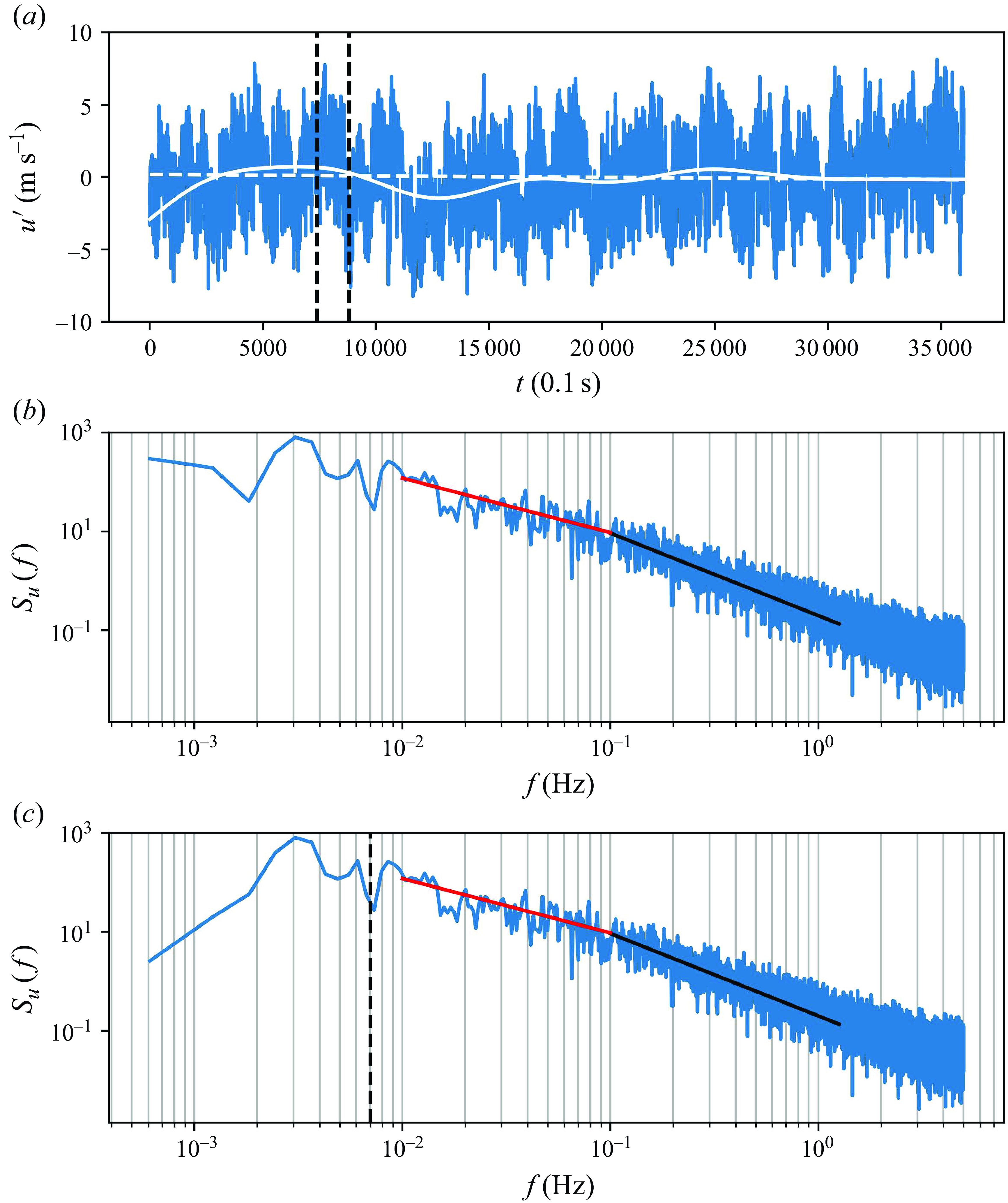
Figure 2. Streamwise velocity time series, $u$
, sampled at 10 Hz from the triaxial sonic anemometer at 12.5 m on 25 September 2020, at 15:00 local time (LT). (a) Turbulent component of streamwise velocity after coordinate rotation: the dashed white line shows the linear fit, the solid white line represents high-pass filtered low-frequency signals that are nonlinear, and the vertical dashed black lines mark the filter size for the high-pass method. (b) Energy spectrum of
$u$
, sampled at 10 Hz from the triaxial sonic anemometer at 12.5 m on 25 September 2020, at 15:00 local time (LT). (a) Turbulent component of streamwise velocity after coordinate rotation: the dashed white line shows the linear fit, the solid white line represents high-pass filtered low-frequency signals that are nonlinear, and the vertical dashed black lines mark the filter size for the high-pass method. (b) Energy spectrum of $u$
after linear detrending: the solid red line and solid black line represent
$u$
after linear detrending: the solid red line and solid black line represent $f^{-1}$
and
$f^{-1}$
and $f^{-5/3}$
scalings, respectively. (c) The energy spectrum of
$f^{-5/3}$
scalings, respectively. (c) The energy spectrum of $u$
after high-pass filtering: the vertical dashed black line indicates the cut-off frequency corresponding to a 2000 m wavelength, for which the filter size is 142 s.
$u$
after high-pass filtering: the vertical dashed black line indicates the cut-off frequency corresponding to a 2000 m wavelength, for which the filter size is 142 s.
A common method in micrometeorology is linear detrending, where the line of best fit over the averaging period (dashed white line in figure 2 a) is subtracted from the original time series. While primarily affecting the low-frequency part of the signal, linear detrending can impact all frequencies and introduce oscillations at higher frequencies (Moncrieff et al. Reference Moncrieff, Clement, Finnigan and Meyers2004).
Alternatively, high-pass filtering can isolate low-frequency signals by convolving the original data with a transfer function in the frequency domain, a method often used in post-processing (Nickels et al. Reference Nickels, Marusic, Hafez and Chong2005; Metzger et al. Reference Metzger, McKeon and Holmes2007; Hutchins et al. Reference Hutchins, Chauhan, Marusic, Monty and Klewicki2012). However, determining a clear cut-off frequency to separate turbulent motions from long-term trends is challenging, posing a risk of filtering out low-wavenumber turbulent motions. A tenth-order Butterworth filter is applied in this work, with a cut-off frequency equivalent to a 2000 m cut-off wavelength. It translates to filter size 100–350 s that varies with mean wind speed at different levels. Those sizes align closely with the observed time period of low-frequency signals in the time series (indicated by the two vertical lines in figure 2 a). This filter size is consistent with previous turbulent boundary layer studies that selected 180 s in Hutchins et al. (Reference Hutchins, Chauhan, Marusic, Monty and Klewicki2012) and 181.8 s in Puccioni et al. (Reference Puccioni, Calaf, Pardyjak, Hoch, Morrison, Perelet and Iungo2023).
As shown in figure 2(b), the linear detrended streamwise velocity energy spectrum $S_u(f)$
levels off as
$S_u(f)$
levels off as $f \to 0$
. In contrast, the high-pass filtered
$f \to 0$
. In contrast, the high-pass filtered $S_u(f)$
shows more removal of low-frequency content (very-large-scale motions) than linear detrending, with a much faster decay as
$S_u(f)$
shows more removal of low-frequency content (very-large-scale motions) than linear detrending, with a much faster decay as $f \to 0$
, as expected (see figure 2
c). Nevertheless, the best method depends on site conditions. Therefore, both methods are initially applied, and a comparison is performed to ensure the derived AEM coefficients are not sensitive to the detrending approach.
$f \to 0$
, as expected (see figure 2
c). Nevertheless, the best method depends on site conditions. Therefore, both methods are initially applied, and a comparison is performed to ensure the derived AEM coefficients are not sensitive to the detrending approach.
2.3.4. Turbulence statistics
After detrending, time averaging of all instantaneous data is conducted to obtain first the mean component and then the turbulent fluctuations as $u^\prime = u-\overline {u}$
,
$u^\prime = u-\overline {u}$
, $v^\prime = v-\overline {v}$
,
$v^\prime = v-\overline {v}$
, $w^\prime = w-\overline {w}$
and
$w^\prime = w-\overline {w}$
and $T^\prime = T-\overline {T}$
, where
$T^\prime = T-\overline {T}$
, where $T$
is the air temperature. The Reynolds stress methods and profile methods are two conventional approaches to estimating the friction velocity in the ASL and those two methods will also be compared for reference.
$T$
is the air temperature. The Reynolds stress methods and profile methods are two conventional approaches to estimating the friction velocity in the ASL and those two methods will also be compared for reference.
-
(i) Reynolds stress method. In an ideal ASL that is high Reynolds number, stationary, planar homogeneous, lacking subsidence and characterized by a zero mean pressure gradient, the momentum fluxes must be invariant to variations in
$z$
. To test the constant flux layer assumption and determine
$u_*$
to be used as a normalizing velocity in the AEM, a local friction velocity is defined as(2.1)
\begin{equation} u_* = \left[\overline {u^\prime w^\prime }^{2}+\overline {v^\prime w^\prime }^{2}\right]^{1/4}. \end{equation}
-
(ii) Profile method. Another approach to estimating
$u_*$
is based on the logarithmic law of the mean velocity as shown in (1.1). This technique, known as the Clauser chart method (Clauser Reference Clauser1956), is commonly used by boundary layer experimentalists. Measurements of the mean velocity profile can be used to estimate the friction velocity by fitting the measured
$\overline {u}$
against
$\ln (z)$
. To do so, it is necessary to identify the beginning and ending points that follow a log-linear relation, which can involve some subjectivity. The magnitude of the friction velocity is directly related to the choice of the von Kármán constant (Kendall & Koochesfahani Reference Kendall and Koochesfahani2008).


Agreement between these two methods is also used when identifying the span of the ASL.
2.4. Data selection
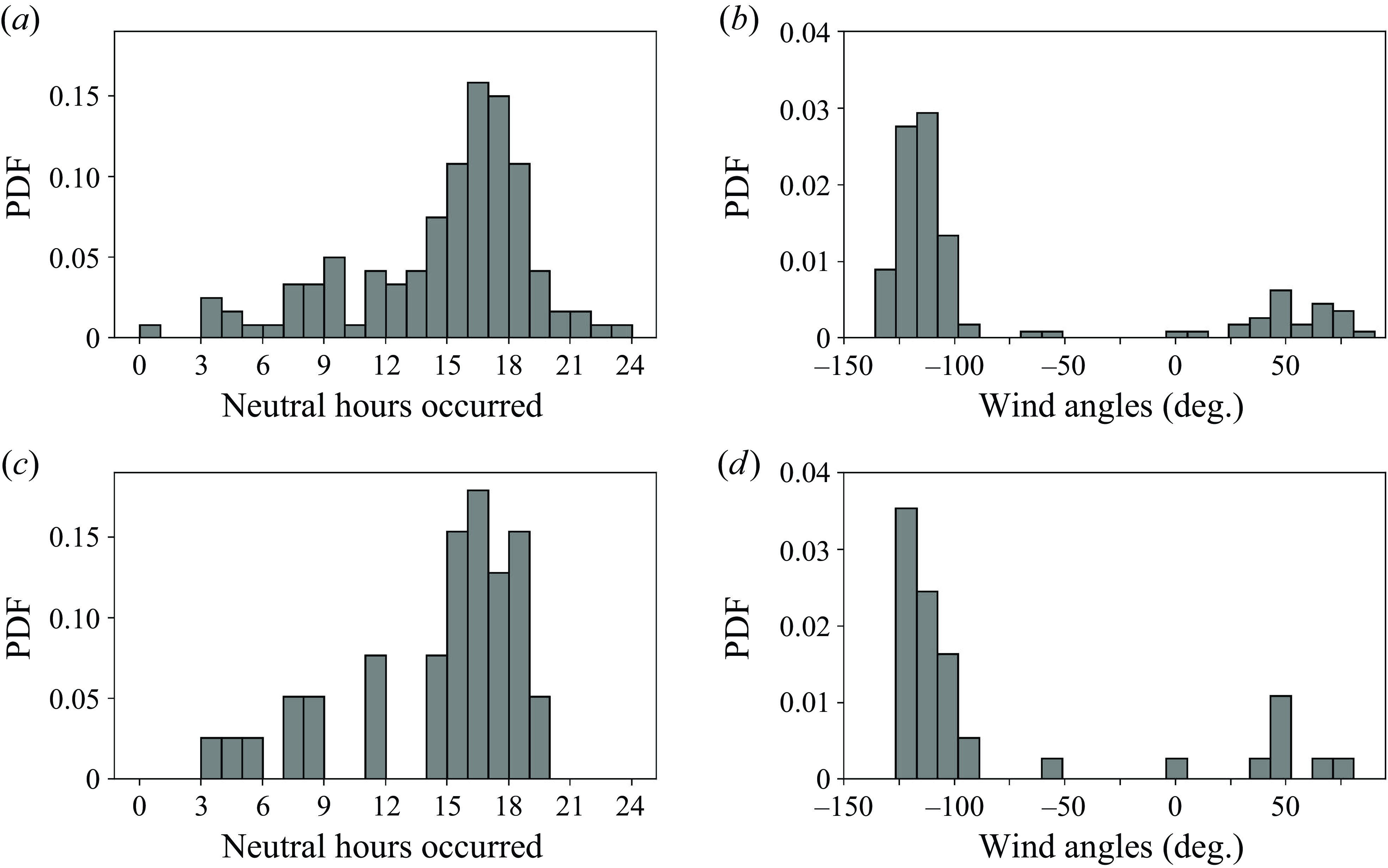
Figure 3. The PDFs of the 120 near-neutral cases (a) by time of day, and (b) by wind angles, at 16.5 m relative to true north, with positive values denoting clockwise, negative values anticlockwise, and 0 denoting northerly wind. Neutral conditions are identified during hours when $|z_{mean}/L_{median}|\lt 0.1$
is satisfied. The PDFs of the 39 post-screening near-neutral cases: (c) by time of day, and (d) by wind angles. Here, (c) and (d) are shown to facilitate comparisons before and after data quality control, with the data quality control discussed in detail in § 3.2.2.
$|z_{mean}/L_{median}|\lt 0.1$
is satisfied. The PDFs of the 39 post-screening near-neutral cases: (c) by time of day, and (d) by wind angles. Here, (c) and (d) are shown to facilitate comparisons before and after data quality control, with the data quality control discussed in detail in § 3.2.2.
From the 210 days of data recorded, the focus is placed on a subset that is approximately neutrally stratified. The stability of the surface layer is characterized by the stability parameter $|z/L|$
, where near-neutral conditions are defined as
$|z/L|$
, where near-neutral conditions are defined as $|z/L| \lt 0.1$
. The local Obukhov length
$|z/L| \lt 0.1$
. The local Obukhov length $L$
is calculated as
$L$
is calculated as $L = -\overline {T} u_*^3/ (\kappa g\, \overline {w'T'} )$
, where
$L = -\overline {T} u_*^3/ (\kappa g\, \overline {w'T'} )$
, where $g$
is the gravitational acceleration, and the time-averaged sonic temperature
$g$
is the gravitational acceleration, and the time-averaged sonic temperature $\overline {T}$
is assumed to be a good approximation to the virtual temperature
$\overline {T}$
is assumed to be a good approximation to the virtual temperature $\theta _v$
. Since multiple measurement levels are considered, the stability parameter is calculated as
$\theta _v$
. Since multiple measurement levels are considered, the stability parameter is calculated as $z_{mean}/L_{median},$
where
$z_{mean}/L_{median},$
where $z_{mean}$
is the geometric mean of the sensor heights, and
$z_{mean}$
is the geometric mean of the sensor heights, and $L_{median}$
is the median value of the local Obukhov length
$L_{median}$
is the median value of the local Obukhov length $L$
across the considered levels. This choice of using the median Obukhov length (
$L$
across the considered levels. This choice of using the median Obukhov length ( $L_{median}$
) and the geometric mean of sensor heights (
$L_{median}$
) and the geometric mean of sensor heights ( $z_{mean}$
) is consistent with the methodology outlined in Andreas et al. (Reference Andreas, Claffy, Jordan, Fairall, Guest, Persson and Grachev2006). This step results in 142 cases remaining. The following criteria are used for further data selection to be consistent with previous ASL studies (Li & Bou-Zeid Reference Li and Bou-Zeid2011).
$z_{mean}$
) is consistent with the methodology outlined in Andreas et al. (Reference Andreas, Claffy, Jordan, Fairall, Guest, Persson and Grachev2006). This step results in 142 cases remaining. The following criteria are used for further data selection to be consistent with previous ASL studies (Li & Bou-Zeid Reference Li and Bou-Zeid2011).
-
(i) Wind must face the sonic anemometers. The angles between the time-mean wind direction and the sonic anemometers have to be smaller than 120
$^\circ$
such that the interference and data contamination from the anemometer arms, tripods and other supporting structures are minimized, which further narrows down the runs to 139. -
(ii) The turbulence intensity (
$\sigma _u/\overline {u}$
) must be less than 0.5 to justify the use of Taylor’s frozen turbulence hypothesis (Taylor Reference Taylor1938), leading to 134 cases remaining.


After applying the above screening procedures and removing cases with pressure measurement errors associated with the gas analyser, 120 cases are retained for further analysis. Figure 3(a) illustrates the probability density function (PDF) of near-neutral conditions, showing that a neutrally stratified ASL can occur throughout the day, peaking at approximately 16:00 LT. The wind is consistently dominated by a west-south-westerly wind direction (as shown in figure 3 b), with few instances of wind from the east-north-east, likely occurring at night.
3. Results
3.1. Determination of the ISL
The local friction velocity computed using (2.1) is investigated first. Figure 4(a) illustrates the vertical distribution of local $u_*(z)$
and their deviations from the vertical average across all 12 levels (
$u_*(z)$
and their deviations from the vertical average across all 12 levels ( $\langle u^{all}_* (z ) \rangle$
, where the angle brackets indicate vertical average). Notably, the friction velocity at the lowermost four levels exhibits significant deviations from the vertical average with increasing trend in
$\langle u^{all}_* (z ) \rangle$
, where the angle brackets indicate vertical average). Notably, the friction velocity at the lowermost four levels exhibits significant deviations from the vertical average with increasing trend in $z$
. Three potential explanations are considered for this observation. First, the lower four levels are mounted on a separate 10 m tower, located approximately 10 m from the 62 m tower, as shown in figure 1(b). Despite the flat and aerodynamically homogeneous surface cover, variations in tower placement may influence turbulent momentum flux measurements near the ground. Second, although the sagebrush is relatively short (tens of centimetres) and the lowest anemometer level is at 1.2 m, the
$z$
. Three potential explanations are considered for this observation. First, the lower four levels are mounted on a separate 10 m tower, located approximately 10 m from the 62 m tower, as shown in figure 1(b). Despite the flat and aerodynamically homogeneous surface cover, variations in tower placement may influence turbulent momentum flux measurements near the ground. Second, although the sagebrush is relatively short (tens of centimetres) and the lowest anemometer level is at 1.2 m, the $z_0$
value derived from the log mean profile has median value approximately 0.08 m. According to Garrett (Reference Garrett1994), the roughness sublayer’s height can be 10–150 times
$z_0$
value derived from the log mean profile has median value approximately 0.08 m. According to Garrett (Reference Garrett1994), the roughness sublayer’s height can be 10–150 times $z_0$
. Assuming a factor of 100 times the roughness length (i.e. 7 m), the roughness sublayer would extend just above the 6 m level. Finally, volume averaging by the sonic anemometer path length (10–15 cm) has a disproportionate impact on the vertical velocity at levels close to the ground, leading to an underestimation of the covariance (and thus friction velocity) at those levels. Therefore, the analysis here excludes the bottom four levels when defining the ISL.
$z_0$
. Assuming a factor of 100 times the roughness length (i.e. 7 m), the roughness sublayer would extend just above the 6 m level. Finally, volume averaging by the sonic anemometer path length (10–15 cm) has a disproportionate impact on the vertical velocity at levels close to the ground, leading to an underestimation of the covariance (and thus friction velocity) at those levels. Therefore, the analysis here excludes the bottom four levels when defining the ISL.
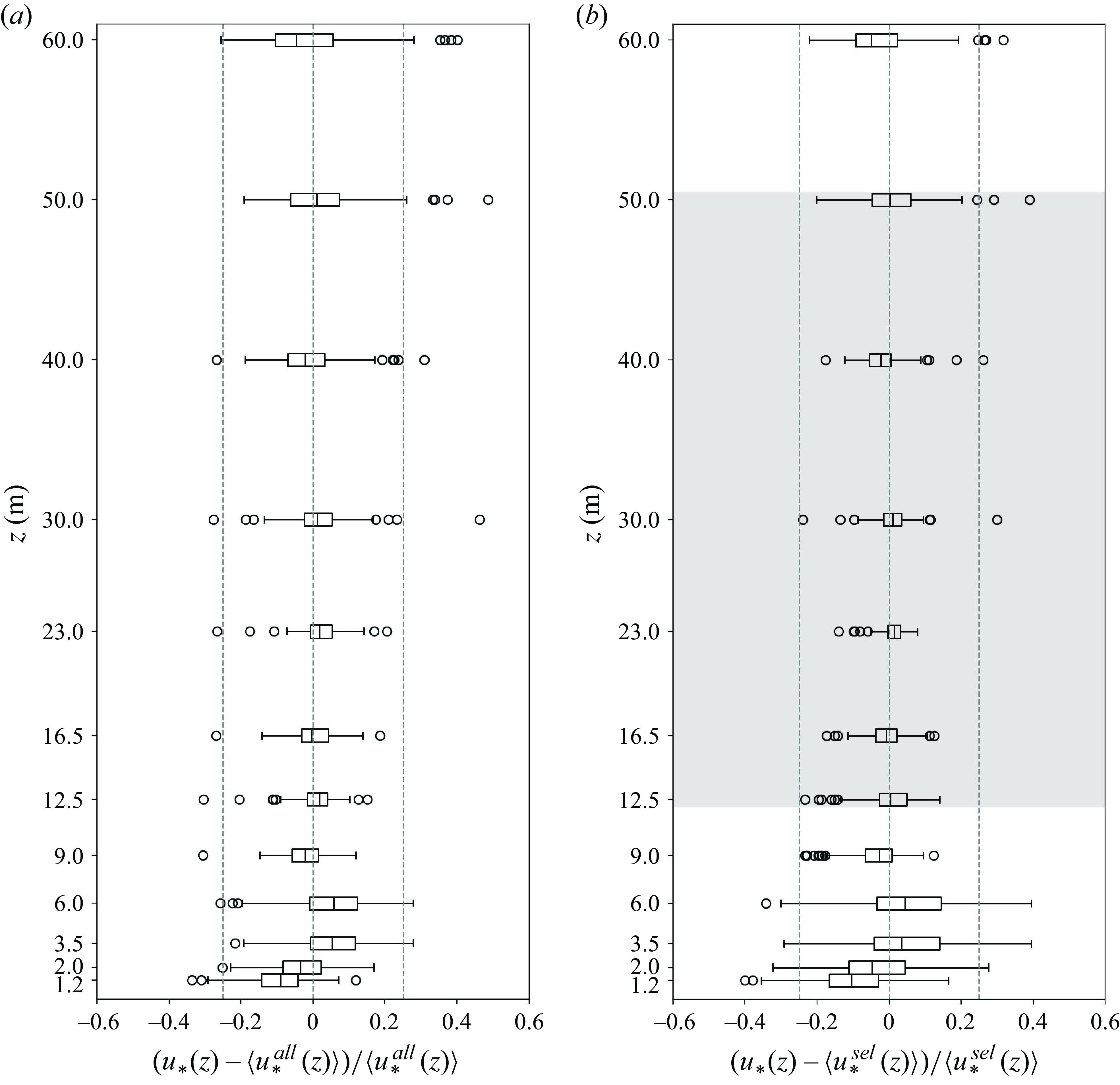
Figure 4. Deviation of locally measured friction velocity from the vertical mean averaged across (a) all twelve levels and (b) the six levels within the ISL for the linear detrended measurements. Box plot interpretation: from left to right, lines signify the minimum, first quartile, median, third quartile and maximum values. Black open circles denote outliers. Vertical dashed lines are set at $-0.25, 0, 0.25$
. The grey shaded region highlights the ISL identified between 12.5 m and 50 m, which is the operational range used in evaluating the AEM. The terms
$-0.25, 0, 0.25$
. The grey shaded region highlights the ISL identified between 12.5 m and 50 m, which is the operational range used in evaluating the AEM. The terms $ \langle u_*^{all}(z)\rangle$
and
$ \langle u_*^{all}(z)\rangle$
and $\langle u_*^{sel}(z)\rangle$
represent the friction velocities averaged over all twelve levels and the six shaded levels, respectively.
$\langle u_*^{sel}(z)\rangle$
represent the friction velocities averaged over all twelve levels and the six shaded levels, respectively.
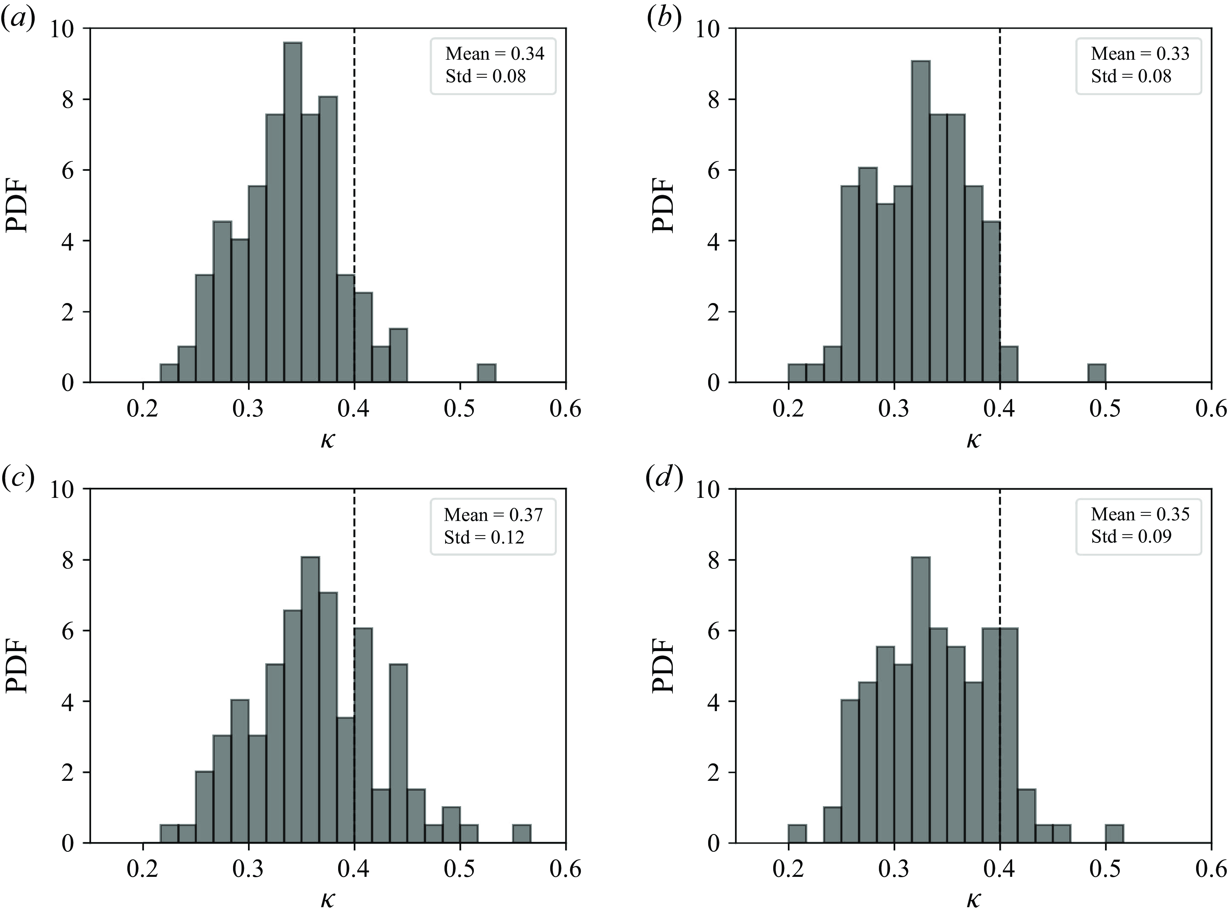
Figure 5. The PDFs for the inferred $\kappa$
values using the mean horizontal velocity from the following levels: (a) 9–50 m, (b) 9–60 m, (c) 12.5–50 m, (d) 12.5–60 m. Vertical dashed lines indicate
$\kappa$
values using the mean horizontal velocity from the following levels: (a) 9–50 m, (b) 9–60 m, (c) 12.5–50 m, (d) 12.5–60 m. Vertical dashed lines indicate $\kappa=0.4$
. The computed means and standard deviations of the fitted
$\kappa=0.4$
. The computed means and standard deviations of the fitted $\kappa$
are shown.
$\kappa$
are shown.
The remaining eight levels, from 9 m to 60 m, show consistent local $u_*$
vertical distribution. To test whether all these eight levels are within the ISL, (1.1) is further applied to fit a friction velocity
$u_*$
vertical distribution. To test whether all these eight levels are within the ISL, (1.1) is further applied to fit a friction velocity $u_*^{fit}$
, assuming
$u_*^{fit}$
, assuming $\kappa=0.4$
. The
$\kappa=0.4$
. The $u_*^{fit}$
value is consistently 10–20 % higher than the local
$u_*^{fit}$
value is consistently 10–20 % higher than the local $u_*(z)$
at these eight levels, implying that the measured turbulent momentum flux and mean velocity at these levels are not entirely consistent with a logarithmic mean velocity profile with
$u_*(z)$
at these eight levels, implying that the measured turbulent momentum flux and mean velocity at these levels are not entirely consistent with a logarithmic mean velocity profile with $\kappa=0.4$
.
$\kappa=0.4$
.
To identify data consistent with a logarithmic mean velocity profile with $\kappa$
close to 0.4, the local
$\kappa$
close to 0.4, the local $u_*$
is used to fit
$u_*$
is used to fit $\kappa$
. Using the remaining eight levels (ranging from 9 m to 60 m), four scenarios for fitting
$\kappa$
. Using the remaining eight levels (ranging from 9 m to 60 m), four scenarios for fitting $\kappa$
are tested: (a) using data from 9 m to 50 m; (b) using data from 9 m to 60 m; (c) using data from 12.5 m to 50 m; and (d) using data from 12.5 m to 60 m. The PDFs of the inferred
$\kappa$
are tested: (a) using data from 9 m to 50 m; (b) using data from 9 m to 60 m; (c) using data from 12.5 m to 50 m; and (d) using data from 12.5 m to 60 m. The PDFs of the inferred $\kappa$
values are shown in figure 5 for all these scenarios. The results indicate that only when using data from 12.5 m to 50 m does the fitted
$\kappa$
values are shown in figure 5 for all these scenarios. The results indicate that only when using data from 12.5 m to 50 m does the fitted $\kappa$
have mean close to 0.4 and exhibit a quasi-Gaussian distribution in the spread, while other scenarios produce
$\kappa$
have mean close to 0.4 and exhibit a quasi-Gaussian distribution in the spread, while other scenarios produce $\kappa$
values that either deviate largely from 0.4 or do not follow a Gaussian distribution in their spread. The same analysis performed on high-pass filtered data produces results similar to those from the linearly detrended data, and are thus not presented.
$\kappa$
values that either deviate largely from 0.4 or do not follow a Gaussian distribution in their spread. The same analysis performed on high-pass filtered data produces results similar to those from the linearly detrended data, and are thus not presented.
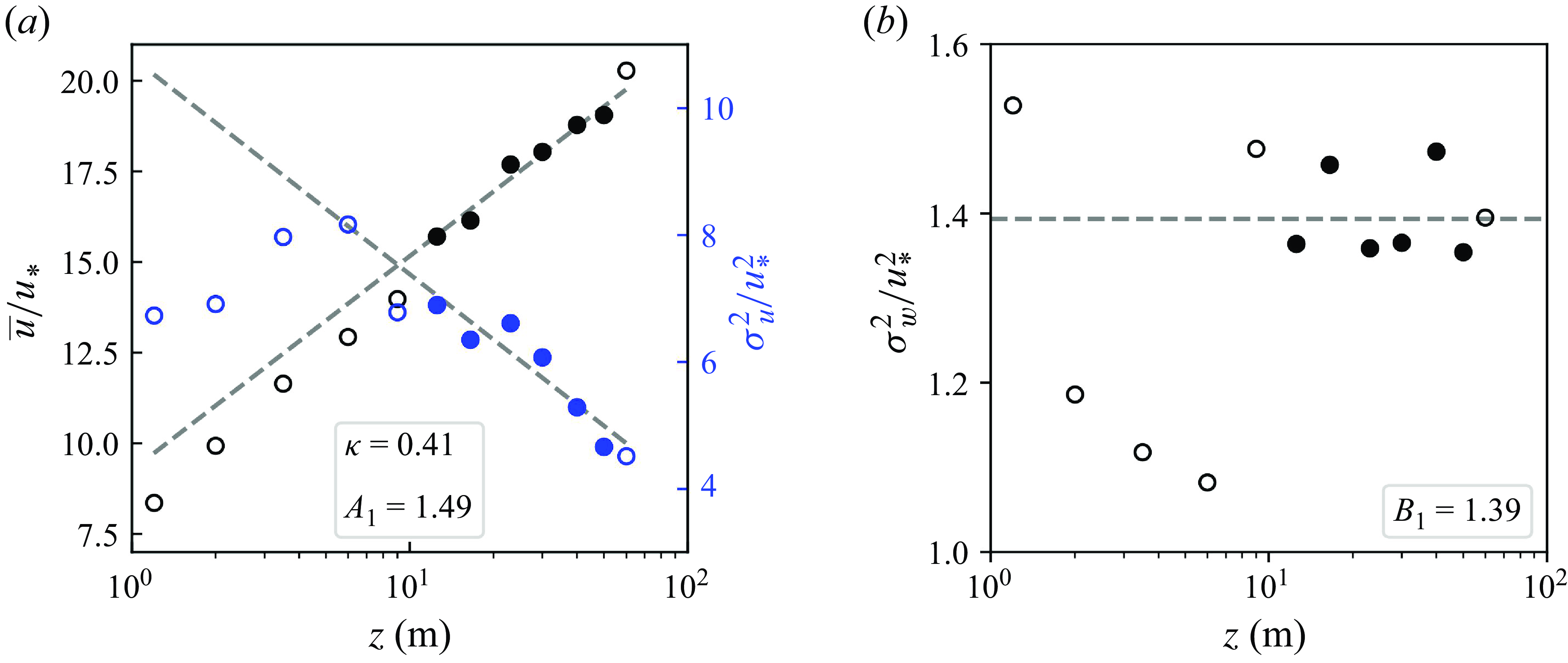
Figure 6. Fitting $\kappa$
,
$\kappa$
, $A_1$
and
$A_1$
and $B_2$
with high-pass filtered data on 25 September 2020, at 15:00 LT: (a) the mean velocity profile (in black), and the streamwise velocity variance profile (in blue); (b) the vertical velocity variance profile. Closed circles indicate the selected data within the ISL. Dashed grey lines denote the linear regression based on the selected data within the ISL. Insets show the results of the fitting.
$B_2$
with high-pass filtered data on 25 September 2020, at 15:00 LT: (a) the mean velocity profile (in black), and the streamwise velocity variance profile (in blue); (b) the vertical velocity variance profile. Closed circles indicate the selected data within the ISL. Dashed grey lines denote the linear regression based on the selected data within the ISL. Insets show the results of the fitting.
Based on this analysis of local $u_*$
, the data between 12.5 m and 50 m are selected for further analysis of the AEM, and this range is treated as the ISL (with the deviation of the locally measured
$u_*$
, the data between 12.5 m and 50 m are selected for further analysis of the AEM, and this range is treated as the ISL (with the deviation of the locally measured $u_*$
from their vertical average shown in figure 4
b). The friction velocity used for normalization in the following analysis is the vertically averaged friction velocity across this range (
$u_*$
from their vertical average shown in figure 4
b). The friction velocity used for normalization in the following analysis is the vertically averaged friction velocity across this range ( $\langle u^{sel}_* (z ) \rangle$
).
$\langle u^{sel}_* (z ) \rangle$
).
3.2. Magnitude of the turbulent velocity fluctuations
3.2.1. Estimation of
$\kappa$
,
$A_1$
and
$B_2$
in the ASL


With $u_*$
and
$u_*$
and $\sigma _u^{2}$
within the ISL measured, a linear regression is conducted to derive the values of
$\sigma _u^{2}$
within the ISL measured, a linear regression is conducted to derive the values of $A_1$
by fitting
$A_1$
by fitting $\sigma _u^{2}$
to
$\sigma _u^{2}$
to $\ln (z)$
utilizing (1.2). Notably, this fitting method for obtaining
$\ln (z)$
utilizing (1.2). Notably, this fitting method for obtaining $A_1$
does not require direct measurement of
$A_1$
does not require direct measurement of $\delta$
, but cannot be used to infer the
$\delta$
, but cannot be used to infer the $B_1$
constant of the AEM. Figure 6(a) demonstrates one such linear regression for the hour 15:00 LT on 25 September 2020, detrended by high-pass filtering. Note that only the closed circles are used for regression because they are situated in the ISL. The logarithmic mean velocity profile is also shown for comparison. The results indicate that the fitted
$B_1$
constant of the AEM. Figure 6(a) demonstrates one such linear regression for the hour 15:00 LT on 25 September 2020, detrended by high-pass filtering. Note that only the closed circles are used for regression because they are situated in the ISL. The logarithmic mean velocity profile is also shown for comparison. The results indicate that the fitted $\kappa$
(
$\kappa$
( $=0.41$
) is very close to the accepted 0.4 value. Moreover, the
$=0.41$
) is very close to the accepted 0.4 value. Moreover, the $\sigma _u^{2}$
profile aligns with AEM predictions, confirming the logarithmic dependence on
$\sigma _u^{2}$
profile aligns with AEM predictions, confirming the logarithmic dependence on $z$
of streamwise velocity variance within the ISL (highlighted by closed circles) at a very high Reynolds number.
$z$
of streamwise velocity variance within the ISL (highlighted by closed circles) at a very high Reynolds number.
To estimate $ B_2$
in (1.3),
$ B_2$
in (1.3), $ \sigma _w^{2}$
is fitted against the local
$ \sigma _w^{2}$
is fitted against the local $ u_*^{2}$
within the ISL, and the resulting slope is retrieved. For example, a
$ u_*^{2}$
within the ISL, and the resulting slope is retrieved. For example, a $ B_2$
value 1.39 is obtained for the hour 15:00 LT on 25 September 2020, as can be seen from figure 6(b). While similar values for
$ B_2$
value 1.39 is obtained for the hour 15:00 LT on 25 September 2020, as can be seen from figure 6(b). While similar values for $B_2$
(i.e. approximately 1.4) have been observed in the ASL literature (Yang & Bo Reference Yang and Bo2018), they are lower than the theoretically predicted value 1.65 for an idealized infinite Reynolds number case. The value 1.65 can be obtained by considering the vertical velocity energy spectrum
$B_2$
(i.e. approximately 1.4) have been observed in the ASL literature (Yang & Bo Reference Yang and Bo2018), they are lower than the theoretically predicted value 1.65 for an idealized infinite Reynolds number case. The value 1.65 can be obtained by considering the vertical velocity energy spectrum $ E_{ww} (k)$
, which consists of a flat energy-containing region spanning wavenumbers from
$ E_{ww} (k)$
, which consists of a flat energy-containing region spanning wavenumbers from $ k=0$
to
$ k=0$
to $ k=k_a$
(energy splashing region) and an inertial subrange from
$ k=k_a$
(energy splashing region) and an inertial subrange from $ k=k_a$
to
$ k=k_a$
to $ k=\infty$
, where
$ k=\infty$
, where $ k_a = (kz)^{-1}$
represents the transition wavenumber. Assuming a balance between TKE production and dissipation, the normalized vertical velocity variance is given by
$ k_a = (kz)^{-1}$
represents the transition wavenumber. Assuming a balance between TKE production and dissipation, the normalized vertical velocity variance is given by $ (\sigma _w/u_*)^{2}=(5/2) C_{o,w}$
, with
$ (\sigma _w/u_*)^{2}=(5/2) C_{o,w}$
, with $ C_{o,w}=0.65$
as the Kolmogorov constant for the one-dimensional vertical velocity spectrum in the inertial subrange. Thus for such an idealized case, this relation predicts
$ C_{o,w}=0.65$
as the Kolmogorov constant for the one-dimensional vertical velocity spectrum in the inertial subrange. Thus for such an idealized case, this relation predicts $ B_2 = 1.65$
. In the area calculation of
$ B_2 = 1.65$
. In the area calculation of $ E_{ww}$
,
$ E_{ww}$
, $ (3/2) C_{o,w}$
out of the total
$ (3/2) C_{o,w}$
out of the total $ (5/2) C_{o,w}$
originates from extending the inertial subrange from
$ (5/2) C_{o,w}$
originates from extending the inertial subrange from $ k=k_a$
to
$ k=k_a$
to $ k=\infty$
, while the remaining
$ k=\infty$
, while the remaining $ C_{o,w}$
comes from the large eddies (i.e. those with scales larger than
$ C_{o,w}$
comes from the large eddies (i.e. those with scales larger than $ 1/k_a$
). Therefore, the reduced
$ 1/k_a$
). Therefore, the reduced $ B_2$
observed here can potentially be attributed to sampling limitations. Specifically, the 10 Hz sampling frequency and path-averaging effects of the anemometer may disproportionately under-resolve the inertial subrange components of the vertical velocity (
$ B_2$
observed here can potentially be attributed to sampling limitations. Specifically, the 10 Hz sampling frequency and path-averaging effects of the anemometer may disproportionately under-resolve the inertial subrange components of the vertical velocity ( $ w$
) compared to its longitudinal (
$ w$
) compared to its longitudinal ( $ u$
) counterpart.
$ u$
) counterpart.
To assess the consistency of the logarithmic behaviour of the streamwise velocity and associated AEM coefficients in the near-neutral ASL, the same fitting procedures are applied across all 120 neutral cases. The goodness of fit for (1.1)–(1.3) is quantified using the coefficients of determination ( $R^{2}$
). The comparison of the results between linearly detrended data and high-pass filtered data can be found in table 3. Note that the linear detrending method and the high-pass filtering method give different
$R^{2}$
). The comparison of the results between linearly detrended data and high-pass filtered data can be found in table 3. Note that the linear detrending method and the high-pass filtering method give different $\overline {u}$
,
$\overline {u}$
, $u_*$
and
$u_*$
and $\sigma _u$
. The analysis shows that the mean estimated values of
$\sigma _u$
. The analysis shows that the mean estimated values of $\kappa$
for both methods are similar, yet smaller than 0.4. This result aligns with previous experiments (Andreas et al. Reference Andreas, Claffy, Jordan, Fairall, Guest, Persson and Grachev2006; Marusic et al. Reference Marusic, McKeon, Monkewitz, Nagib, Smits and Sreenivasan2010) and theoretical predictions based on the co-spectral budget (Katul et al. Reference Katul, Porporato, Manes and Meneveau2013), where
$\kappa$
for both methods are similar, yet smaller than 0.4. This result aligns with previous experiments (Andreas et al. Reference Andreas, Claffy, Jordan, Fairall, Guest, Persson and Grachev2006; Marusic et al. Reference Marusic, McKeon, Monkewitz, Nagib, Smits and Sreenivasan2010) and theoretical predictions based on the co-spectral budget (Katul et al. Reference Katul, Porporato, Manes and Meneveau2013), where $ \kappa$
is linked to the Rotta constant – an isotropization parameter associated with rapid distortion theory – and the Kolmogorov constant. However, the fitted values of
$ \kappa$
is linked to the Rotta constant – an isotropization parameter associated with rapid distortion theory – and the Kolmogorov constant. However, the fitted values of $ \kappa$
exhibit substantial variability. Such variability is not uncommon since extensive evidence suggests that
$ \kappa$
exhibit substantial variability. Such variability is not uncommon since extensive evidence suggests that $ \kappa$
is not a universal constant but rather depends on flow conditions even for weak (in)stability effects (Österlund et al. Reference Österlund, Johansson, Nagib and Hites2000; Andreas et al. Reference Andreas, Claffy, Jordan, Fairall, Guest, Persson and Grachev2006; Nagib & Chauhan Reference Nagib and Chauhan2008). Furthermore, the fitted
$ \kappa$
is not a universal constant but rather depends on flow conditions even for weak (in)stability effects (Österlund et al. Reference Österlund, Johansson, Nagib and Hites2000; Andreas et al. Reference Andreas, Claffy, Jordan, Fairall, Guest, Persson and Grachev2006; Nagib & Chauhan Reference Nagib and Chauhan2008). Furthermore, the fitted $B_2$
are relatively consistent between two detrending methods. As a result, the current analysis focuses on
$B_2$
are relatively consistent between two detrending methods. As a result, the current analysis focuses on $A_1$
. The high-pass filtered data exhibit a more robust logarithmic scaling of
$A_1$
. The high-pass filtered data exhibit a more robust logarithmic scaling of $\sigma _ u^{2}$
than the linearly detrended data. This outcome is based on the finding that the linear detrending method yields a wider range of
$\sigma _ u^{2}$
than the linearly detrended data. This outcome is based on the finding that the linear detrending method yields a wider range of $R^{2}$
values, with average 0.67 and standard deviation 0.32. In contrast, the high-pass filtering yields a higher mean (0.81) and a lower standard deviation (0.23) in
$R^{2}$
values, with average 0.67 and standard deviation 0.32. In contrast, the high-pass filtering yields a higher mean (0.81) and a lower standard deviation (0.23) in $R^{2}$
scores. Moreover, the derived
$R^{2}$
scores. Moreover, the derived $A_1$
values of linear-detrended data exhibit significant variability, often departing considerably from the conventional range 1–1.3, and frequently resulting in negative
$A_1$
values of linear-detrended data exhibit significant variability, often departing considerably from the conventional range 1–1.3, and frequently resulting in negative $A_1$
values (31.63 % and 9.18 % negative occurrence for linear detrending and high-pass filtering, respectively). The potential reasons for this deviation are discussed next.
$A_1$
values (31.63 % and 9.18 % negative occurrence for linear detrending and high-pass filtering, respectively). The potential reasons for this deviation are discussed next.
Table 3. Comparison of the fitted values of the von Kármán constant ( $\kappa$
), AEM coefficient (
$\kappa$
), AEM coefficient ( $A_1$
) and
$A_1$
) and $B_2$
between group I (linear-detrended data), group II (high-pass filtered data), and group III (high-pass filtered data with
$B_2$
between group I (linear-detrended data), group II (high-pass filtered data), and group III (high-pass filtered data with $Re_{\tau } \gt 4 \times 10^7$
and
$Re_{\tau } \gt 4 \times 10^7$
and $R^{2} \gt 0.6$
). Here,
$R^{2} \gt 0.6$
). Here, $B_2$
is estimated from the slope of
$B_2$
is estimated from the slope of $\sigma _w^{2}$
over
$\sigma _w^{2}$
over $u_*^{2}$
within the ISL. The
$u_*^{2}$
within the ISL. The $R^{2}$
values represent the coefficients of determination of the fits. The first two rows display results from double rotation, while the bottom two rows are from planar fit.
$R^{2}$
values represent the coefficients of determination of the fits. The first two rows display results from double rotation, while the bottom two rows are from planar fit.
Given an averaging period of 1 hour, the turbulence data might experience unsteadiness associated with larger-scale meteorological influences such as static pressure gradients. According to Högström et al. (Reference Högström, Hunt and Smedman2002), ‘inactive’ turbulence becomes more significant as the pressure gradient increases, potentially obscuring the scaling behaviour predicted by the AEM. While the linear-detrending method only removes the mean trend, it might not sufficiently eliminate the (nonlinear) large-scale meteorological influences, potentially leading to negative fitted values of $A_1$
. This underscores the importance of removing larger-scale meteorological influences in ASL data when comparing them to a canonical turbulent boundary layer. Furthermore, sensitivity tests indicate that the fitting outcomes are not sensitive to the choice of the cut-off frequency in the 100–200 s range for the high-pass filtering method. Consequently, the following analysis focuses on high-pass filtered data.
$A_1$
. This underscores the importance of removing larger-scale meteorological influences in ASL data when comparing them to a canonical turbulent boundary layer. Furthermore, sensitivity tests indicate that the fitting outcomes are not sensitive to the choice of the cut-off frequency in the 100–200 s range for the high-pass filtering method. Consequently, the following analysis focuses on high-pass filtered data.
Finally, table 3 presents results from both the double rotation and planar fit methods, showing essentially no differences in the fitted $\kappa$
values. The fitted
$\kappa$
values. The fitted $A_1$
and
$A_1$
and $B_1$
differ between the two methods. However, as will be seen in § 3.2.2, once data quality control is applied, the difference between the double rotation and planar fit methods becomes much smaller even for fitted
$B_1$
differ between the two methods. However, as will be seen in § 3.2.2, once data quality control is applied, the difference between the double rotation and planar fit methods becomes much smaller even for fitted $A_1$
. As such, the following discussion is based primarily on the double rotation method.
$A_1$
. As such, the following discussion is based primarily on the double rotation method.
3.2.2. Objective data quality control
To understand the variations in the fitted $A_1$
, key factors that influence data quality are investigated, including statistical fitting performance, non-stationarity effects, the presence of a constant
$A_1$
, key factors that influence data quality are investigated, including statistical fitting performance, non-stationarity effects, the presence of a constant $\sigma _w$
with height in the ISL, and the Reynolds number effect. Other effects, such as wind turning with height and wind shear, are shown to be very small and are thus not considered.
$\sigma _w$
with height in the ISL, and the Reynolds number effect. Other effects, such as wind turning with height and wind shear, are shown to be very small and are thus not considered.
-
(i) Fitting performance. Before discussing the fitted coefficients of the AEM to the data here, it is necessary to evaluate the goodness of the logarithmic scaling for
$\sigma _u^{2}$
. The coefficient of determination (
$R^{2}$
) from the logarithmic fitting is examined, and anomalous cases less than a threshold are filtered out to ensure that only high-quality fits are considered when evaluating
$A_1$
. -
(ii) Non-stationarity effects. Stationarity is a necessary condition for the AEM and for the identification of the ISL. Two indices of stationarity (IST) defined here are in essence similar to the steady-state test described by Foken & Wichura (Reference Foken and Wichura1996):
(3.1)
\begin{equation} {IST_{wspd}} = \displaystyle\frac {\left|\frac {1}{12} \sum _{i=1}^{12} {\sigma _u^i}^{2}-\sigma _u^{2}\right|}{\sigma _u^{2}}, \end{equation}
(3.2)
\begin{equation} {IST_{wdir}(^\circ )} = {|wdir_{5min}-wdir_{1h}|}_{max}. \end{equation}
In (3.1),
${\sigma _u^i}^{2}$
is the streamwise velocity variance for each 5 min block within the 1 h run, and
$\sigma _u^{2}$
is the variance for the entire hour. In (3.2), the notation
$|\cdot |_{max}$
represents the maximum difference between the wind direction observed at a 5 min interval and the wind direction observed at a 1 h interval, among the 12 individual blocks. When the value of
${IST}$
is small (close to zero), the streamwise velocity time series can be viewed as stationary. As the value of
${IST}$
increases, the non-stationarity effects become significant. According to Moncrieff et al. (Reference Moncrieff, Clement, Finnigan and Meyers2004),
${IST_{wspd}}\lt 30\,\%$
should be achieved to ensure stationarity of the
$u$
time series, and this metric is employed here. -
(iii) Presence of a constant
${\sigma }_w$
. An index
$I_{\sigma _w}=|\sigma _w - \langle \sigma _w\rangle |/\langle \sigma _w\rangle$
is defined to measure the deviation of the vertical velocity standard deviation at each level from its depth-averaged value (
$\langle \sigma _w\rangle$
) across the ISL. A small value suggests that the vertical velocity standard deviation is vertically uniform consistent with the AEM. The necessary conditions for the vertical velocity variance to be invariant with
$z$
in the ISL may be derived from the mean vertical velocity equation for stationary, planar homogeneous flow in the absence of subsidence at very high Reynolds number. For these idealized conditions, the vertical velocity variance is given by(3.3)
\begin{align} \frac {\partial \sigma _w^{2}}{\partial z}=-\left (\frac {1}{\rho }\right )\left (\frac {\partial \overline {P}}{\partial z}\right )-g, \end{align}
where
$\overline {P}$
is the mean pressure. When
$\overline {P}=-\rho g z$
(i.e. hydrostatic),
$\partial \sigma _w^{2}/\partial z=0$
or
$\sigma _w^{2}$
is constant with respect to
$z$
within the ISL. That is, the AEM requires
$\overline {P}$
to be hydrostatic above and beyond the zero-pressure gradient condition needed to ensure a constant turbulent stress with
$z$
. The effects of adverse pressure gradients on
$C_1$
have already been reported in wind tunnels and pipes (Turan et al. Reference Turan, Azad and Kassab1987). In the absence of mean pressure gradients, values of
$C_1$
varying from 0.90 to 0.92 have been reported. Interestingly, for large adverse pressure gradients, a
$-1$
power law was still reported, but values of
$C_1$
as high as 17 were computed (Turan et al. Reference Turan, Azad and Kassab1987). These laboratory experiments underscore connections between the aforementioned constant
$\sigma _w^{2}$
with
$z$
, finite mean pressure gradients, and the numerical values of
$C_1$
and
$A_1$
. -
(iv) Reynolds number. As earlier noted, sufficiently large Reynolds numbers are necessary when applying the AEM, allowing for self-similarity of turbulent structures (Townsend Reference Townsend1976). Numerous studies highlight the importance of high Reynolds numbers in validating the AEM and observing the expected turbulent behaviour (Marusic et al. Reference Marusic, McKeon, Monkewitz, Nagib, Smits and Sreenivasan2010; Smits et al. Reference Smits, McKeon and Marusic2011; Banerjee & Katul Reference Banerjee and Katul2013; Huang & Katul Reference Huang and Katul2022). Therefore, the dependency of fitted
$A_1$
on
$Re_{\tau }$
is also investigated. To calculate a bulk Reynolds number analogous to what is reported in laboratory studies,
$\delta$
must be estimated. No direct measurement of
$\delta$
is available during the experiment, and the boundary layer height is estimated from
$\delta = C_a u_*/f_c$
, where
$C_a$
is a dimensionless empirical constant typically varying between 0.07 and 0.3 (Seibert et al. Reference Seibert, Beyrich, Gryning, Joffre, Rasmussen and Tercier2000). Here,
$C_a=0.1$
is used after examining the streamwise energy spectrum as discussed later, and
$f_c$
is the Coriolis parameter given by
$f_c=2\Omega \sin (\phi )$
, where
$\Omega$
is the angular velocity of the Earth, and
$\phi$
is the latitude of the location (Zilitinkevich Reference Zilitinkevich1972). While we acknowledge that the uncertainties of
$C_a$
can introduce uncertainties in the magnitude of the calculated boundary layer height
$\delta$
and the bulk Reynolds number
$Re_\tau$
, these uncertainties will not alter our main finding.


Before examining how fitted $A_1$
is affected by these individual factors mentioned above, it is noted that these factors are not entirely independent of each other. Figure 7(a) reveals a moderate negative correlation between
$A_1$
is affected by these individual factors mentioned above, it is noted that these factors are not entirely independent of each other. Figure 7(a) reveals a moderate negative correlation between $R^{2}$
and
$R^{2}$
and $\mathrm{IST}_{wspd}$
, indicating that increased non-stationarity in wind speed reduces the quality of the logarithmic fit. A weak negative correlation between
$\mathrm{IST}_{wspd}$
, indicating that increased non-stationarity in wind speed reduces the quality of the logarithmic fit. A weak negative correlation between $R^{2}$
and
$R^{2}$
and $\mathrm{IST}_{wdir}$
suggests a discernible decrease in fit quality with higher wind direction non-stationarity. More dynamically interesting is that higher computed Reynolds numbers (
$\mathrm{IST}_{wdir}$
suggests a discernible decrease in fit quality with higher wind direction non-stationarity. More dynamically interesting is that higher computed Reynolds numbers ( $Re_{\tau }$
) are positively correlated with a better fitting quality (
$Re_{\tau }$
) are positively correlated with a better fitting quality ( $R^{2}$
), agreeing with the basic assumption of the AEM. Non-stationarity in wind speed (
$R^{2}$
), agreeing with the basic assumption of the AEM. Non-stationarity in wind speed ( $\mathrm{IST}_{wspd}$
) is negatively correlated with
$\mathrm{IST}_{wspd}$
) is negatively correlated with $Re_{\tau }$
, and greater deviations in the vertical velocity standard deviation (
$Re_{\tau }$
, and greater deviations in the vertical velocity standard deviation ( $I_{\sigma _w}$
) and higher non-stationarity indices tend to occur at lower Reynolds numbers. Overall, a smaller
$I_{\sigma _w}$
) and higher non-stationarity indices tend to occur at lower Reynolds numbers. Overall, a smaller $Re_{\tau }$
reflects, to some extent, the non-stationarity effect and the absence of a constant
$Re_{\tau }$
reflects, to some extent, the non-stationarity effect and the absence of a constant $\sigma _w$
, all of which implicitly affect the fitting quality for the constants of the AEM at very high
$\sigma _w$
, all of which implicitly affect the fitting quality for the constants of the AEM at very high $Re_{\tau }$
. Therefore, the analysis focuses primarily on the role of
$Re_{\tau }$
. Therefore, the analysis focuses primarily on the role of $Re_{\tau }$
in describing the variations in fitted
$Re_{\tau }$
in describing the variations in fitted $A_1$
values.
$A_1$
values.
Figure 7. (a) Correlation heatmap between $R^{2}$
(coefficient of determination from the logarithmic fitting of the streamwise velocity variance),
$R^{2}$
(coefficient of determination from the logarithmic fitting of the streamwise velocity variance), $\mathrm{IST}_{wspd}$
(non-stationarity index of wind speed),
$\mathrm{IST}_{wspd}$
(non-stationarity index of wind speed), $\mathrm{IST}_{wdir}$
(non-stationarity index of wind direction),
$\mathrm{IST}_{wdir}$
(non-stationarity index of wind direction), $I_{\sigma _w}$
(absolute deviation of vertical velocity standard deviation from its mean across the ISL), and
$I_{\sigma _w}$
(absolute deviation of vertical velocity standard deviation from its mean across the ISL), and $Re_{\tau }$
(the bulk Reynolds number). Note that
$Re_{\tau }$
(the bulk Reynolds number). Note that $\mathrm{IST}_{wspd}$
,
$\mathrm{IST}_{wspd}$
, $\mathrm{IST}_{wdir}$
and
$\mathrm{IST}_{wdir}$
and $I_{\sigma _w}$
are calculated at every height and then averaged across the ISL. (b) Relation between
$I_{\sigma _w}$
are calculated at every height and then averaged across the ISL. (b) Relation between $A_1$
and
$A_1$
and $Re_{\tau }$
. Open circles represent the original 120 neutral cases, while closed circles denote the 39 cases with
$Re_{\tau }$
. Open circles represent the original 120 neutral cases, while closed circles denote the 39 cases with $Re_{\tau }\gt 4 \times 10^7$
and
$Re_{\tau }\gt 4 \times 10^7$
and $R^{2}\gt 0.6$
. The blue line represents the relation between
$R^{2}\gt 0.6$
. The blue line represents the relation between $A_1$
and
$A_1$
and $Re_{\tau }$
as described in Katul et al. (Reference Katul, Banerjee, Cava, Germano and Porporato2016), assuming
$Re_{\tau }$
as described in Katul et al. (Reference Katul, Banerjee, Cava, Germano and Porporato2016), assuming $ A_1 = C_1 = C_{o,u} \kappa ^{-2/3}$
, where
$ A_1 = C_1 = C_{o,u} \kappa ^{-2/3}$
, where $ C_{o,u}$
is the Kolmogorov constant for the one-dimensional streamwise velocity spectrum in the inertial subrange (
$ C_{o,u}$
is the Kolmogorov constant for the one-dimensional streamwise velocity spectrum in the inertial subrange ( $=0.49$
). The red line denotes
$=0.49$
). The red line denotes $A_1=1.25$
.
$A_1=1.25$
.
Figure 7(b) illustrates that the derived $A_1$
values vary appreciably at lower Reynolds numbers but tend to converge asymptotically towards a relatively constant range around 1.25 as
$A_1$
values vary appreciably at lower Reynolds numbers but tend to converge asymptotically towards a relatively constant range around 1.25 as ${Re}_{\tau }$
increases. This suggests that despite the ASL Reynolds numbers being on the order of
${Re}_{\tau }$
increases. This suggests that despite the ASL Reynolds numbers being on the order of $10^7$
, the fitted
$10^7$
, the fitted $A_1$
values remain dependent on the Reynolds number. But here we should again highlight that the Reynolds number effect is correlated with other factors such as non-stationarity, thus this Reynolds number dependence of
$A_1$
values remain dependent on the Reynolds number. But here we should again highlight that the Reynolds number effect is correlated with other factors such as non-stationarity, thus this Reynolds number dependence of $A_1$
cannot be strictly interpreted as the dependence of
$A_1$
cannot be strictly interpreted as the dependence of $A_1$
on the scale separation in turbulent flows (Marusic et al. Reference Marusic, McKeon, Monkewitz, Nagib, Smits and Sreenivasan2010; Smits et al. Reference Smits, McKeon and Marusic2011; Banerjee & Katul Reference Banerjee and Katul2013; Huang & Katul Reference Huang and Katul2022).
$A_1$
on the scale separation in turbulent flows (Marusic et al. Reference Marusic, McKeon, Monkewitz, Nagib, Smits and Sreenivasan2010; Smits et al. Reference Smits, McKeon and Marusic2011; Banerjee & Katul Reference Banerjee and Katul2013; Huang & Katul Reference Huang and Katul2022).
When $Re_{\tau }\gt 4 \times 10^7$
is used as the criterion, 41 cases remain, all of which satisfy
$Re_{\tau }\gt 4 \times 10^7$
is used as the criterion, 41 cases remain, all of which satisfy $\mathrm{IST}_{wspd}\lt 30\,\%$
. To determine an appropriate threshold for
$\mathrm{IST}_{wspd}\lt 30\,\%$
. To determine an appropriate threshold for $R^{2}$
values and identify potential outliers, the interquartile range (IQR) method (Komorowski et al. Reference Komorowski, Marshall, Salciccioli and Crutain2016) is applied. Outliers are defined as values outside the range
$R^{2}$
values and identify potential outliers, the interquartile range (IQR) method (Komorowski et al. Reference Komorowski, Marshall, Salciccioli and Crutain2016) is applied. Outliers are defined as values outside the range $(Q_1 - 1.5 \times \textit{IQR}, Q_3 + 1.5 \times \textit{IQR})$
, where
$(Q_1 - 1.5 \times \textit{IQR}, Q_3 + 1.5 \times \textit{IQR})$
, where $Q_1$
,
$Q_1$
, $Q_3$
are defined as the 25th and 75th percentiles of the data, and
$Q_3$
are defined as the 25th and 75th percentiles of the data, and $\textit{IQR} = Q_3-Q_1$
. For the 41 cases, the IQR analysis of
$\textit{IQR} = Q_3-Q_1$
. For the 41 cases, the IQR analysis of $R^{2}$
values results in
$R^{2}$
values results in $ Q_1 - 1.5 \times \textit{IQR} =0.62$
. Based on this analysis,
$ Q_1 - 1.5 \times \textit{IQR} =0.62$
. Based on this analysis, $R^{2} \gt 0.6$
has been adopted as the threshold for excluding outliers. This removes two outliers, shown as open circles. Therefore, the subsequent analysis focuses on the 39 cases where
$R^{2} \gt 0.6$
has been adopted as the threshold for excluding outliers. This removes two outliers, shown as open circles. Therefore, the subsequent analysis focuses on the 39 cases where $R^{2}\gt 0.6$
and
$R^{2}\gt 0.6$
and $Re_{\tau }\gt 4 \times 10^7$
.
$Re_{\tau }\gt 4 \times 10^7$
.
Table 3 and 4 present the results before and after applying the criteria $Re_{\tau }\gt 4 \times 10^7$
and
$Re_{\tau }\gt 4 \times 10^7$
and $R^{2}\gt 0.6$
. After these quality controls are applied, the mean value of
$R^{2}\gt 0.6$
. After these quality controls are applied, the mean value of $A_1$
changes from 1.25 to 1.22. The mean value of
$A_1$
changes from 1.25 to 1.22. The mean value of $\kappa$
remains consistent (from 0.37 to 0.38), though with a reduced standard deviation. The
$\kappa$
remains consistent (from 0.37 to 0.38), though with a reduced standard deviation. The $R^{2}$
values show marked improvement, and the non-stationarity indices decrease substantially. The vertical variability of
$R^{2}$
values show marked improvement, and the non-stationarity indices decrease substantially. The vertical variability of $\sigma _w$
also decreases from 0.03 to 0.02.
$\sigma _w$
also decreases from 0.03 to 0.02.
Table 4. Comparison of mean and standard deviation (Std) before and after applying the screening $Re_{\tau }\gt 4 \times 10^7$
and
$Re_{\tau }\gt 4 \times 10^7$
and $R^{2}\gt 0.6$
. Variables are defined as in figure 7.
$R^{2}\gt 0.6$
. Variables are defined as in figure 7.

Post-screening, the patterns of near-neutral occurrence hours and wind directions remain consistent with the previous data. Instances that are infrequent pre-screening become even rarer after the screening, while common instances become more frequent (see figure 3
c,d). The double rotation and planar fit methods show even smaller differences (see table 3). The analysis indicates that the variations in $A_1$
are driven primarily by non-stationarity considerations and Reynolds number dependence. However, the variability of
$A_1$
are driven primarily by non-stationarity considerations and Reynolds number dependence. However, the variability of $A_1$
(standard deviation 0.33) remains non-trivial compared to the classical values derived from laboratory experiments, despite all the data quality controls imposed on these ASL measurements. This highlights the complexity of ASL flows, necessitating case-by-case investigations, which will be discussed in § 3.3.2.
$A_1$
(standard deviation 0.33) remains non-trivial compared to the classical values derived from laboratory experiments, despite all the data quality controls imposed on these ASL measurements. This highlights the complexity of ASL flows, necessitating case-by-case investigations, which will be discussed in § 3.3.2.
3.2.3. Effect of stability
In unstable conditions, thermal plumes enhance vertical mixing and modify the turbulent eddy structure. In stable conditions, near-surface turbulence and the residual layer above it progressively decouple with increasing stability, reducing the influence of ABL-scale motions on near-surface turbulence, and diminishing the size of streamwise streaks. In those conditions, near-surface turbulence becomes intermittent (Dupont & Patton Reference Dupont and Patton2022). These modifications can influence the streamwise velocity variance and energy spectra, including the $k^{-1}$
scaling (Banerjee et al. Reference Banerjee, Katul, Salesky and Chamecki2015). In our study,
$k^{-1}$
scaling (Banerjee et al. Reference Banerjee, Katul, Salesky and Chamecki2015). In our study, $\left |z_{mean}/L_{median}\right |\lt 0.1$
is used to select near-neutral cases, which is not a strict condition. Whether the selected cases are still influenced by some remaining buoyancy effects (especially the higher
$\left |z_{mean}/L_{median}\right |\lt 0.1$
is used to select near-neutral cases, which is not a strict condition. Whether the selected cases are still influenced by some remaining buoyancy effects (especially the higher $z$
measurements) is now considered.
$z$
measurements) is now considered.
It is observed that sensible heat flux magnitude ( $|H|$
) shows a strong positive correlation with
$|H|$
) shows a strong positive correlation with $Re_{\tau }$
(correlation coefficient 0.65), indicating that higher sensible heat fluxes tend to be associated with higher Reynolds numbers. Given a constant
$Re_{\tau }$
(correlation coefficient 0.65), indicating that higher sensible heat fluxes tend to be associated with higher Reynolds numbers. Given a constant $C_a$
used in this study, the correlation between sensible heat flux magnitude and
$C_a$
used in this study, the correlation between sensible heat flux magnitude and $Re_{\tau }$
is caused by the friction velocity (
$Re_{\tau }$
is caused by the friction velocity ( $u_*$
). At our site, higher friction velocities are generally associated with higher sensible heat fluxes, maintaining near-neutral stability in the ASL.
$u_*$
). At our site, higher friction velocities are generally associated with higher sensible heat fluxes, maintaining near-neutral stability in the ASL.
Figure 8(a) illustrates the relation between the stability parameter and the fitted $A_1$
. The screening criteria
$A_1$
. The screening criteria $ Re_{\tau }\gt 4 \times 10^7$
and
$ Re_{\tau }\gt 4 \times 10^7$
and $ R^{2} \gt 0.6$
exclude data with stability parameters greater than 0.026 (positive, stable) and less than
$ R^{2} \gt 0.6$
exclude data with stability parameters greater than 0.026 (positive, stable) and less than $-0.05$
(negative, unstable). The remaining data are approximately evenly distributed across the range
$-0.05$
(negative, unstable). The remaining data are approximately evenly distributed across the range $(-0.05, 0.025)$
with no significant trend. This suggests that there is little stability effect on
$(-0.05, 0.025)$
with no significant trend. This suggests that there is little stability effect on $A_1$
after screening. This finding is not sensitive to the criterion
$A_1$
after screening. This finding is not sensitive to the criterion $\left |z_{mean}/L_{median}\right |\lt 0.1$
, which justifies its initial choice for indicating near-neutral conditions.
$\left |z_{mean}/L_{median}\right |\lt 0.1$
, which justifies its initial choice for indicating near-neutral conditions.

Figure 8. Relations between (a) the fitted $A_1$
and (b) the fitted
$A_1$
and (b) the fitted $\kappa$
and stability parameters
$\kappa$
and stability parameters $z_{mean}/L_{median}$
. Vertical dashed lines represent
$z_{mean}/L_{median}$
. Vertical dashed lines represent $z_{mean}/L_{median}=0$
, solid red lines denote the linear regression of the data, grey shadings denote the 95th confidence level, and closed circles denote the 39 cases with
$z_{mean}/L_{median}=0$
, solid red lines denote the linear regression of the data, grey shadings denote the 95th confidence level, and closed circles denote the 39 cases with $Re_{\tau }\gt 4 \times 10^7$
and
$Re_{\tau }\gt 4 \times 10^7$
and $R^{2}\gt 0.6$
. Note that two outliers in (a) and 3 outliers in (b) are not shown, for better visualization. The legends give the correlation coefficients (
$R^{2}\gt 0.6$
. Note that two outliers in (a) and 3 outliers in (b) are not shown, for better visualization. The legends give the correlation coefficients ( $R$
).
$R$
).
In contrast, the influence of stability conditions on the fitted values of $\kappa$
is visible in figure 8(b). Even after applying the stability constraint, the fitted
$\kappa$
is visible in figure 8(b). Even after applying the stability constraint, the fitted $\kappa$
values remain influenced by variations in atmospheric stability. This finding is consistent with Andreas et al. (Reference Andreas, Claffy, Jordan, Fairall, Guest, Persson and Grachev2006), who reported a range of
$\kappa$
values remain influenced by variations in atmospheric stability. This finding is consistent with Andreas et al. (Reference Andreas, Claffy, Jordan, Fairall, Guest, Persson and Grachev2006), who reported a range of $\kappa$
values between 0.2 and 0.6 for
$\kappa$
values between 0.2 and 0.6 for $-0.1 \lt z/L \lt 0.1$
in their figure 6. It is possible to correct the stability effect on
$-0.1 \lt z/L \lt 0.1$
in their figure 6. It is possible to correct the stability effect on $\kappa$
by employing MOST and the Businger–Dyer relation for the stability correction function (Businger Reference Businger1988). After correcting the stability effects, the median value of
$\kappa$
by employing MOST and the Businger–Dyer relation for the stability correction function (Businger Reference Businger1988). After correcting the stability effects, the median value of $\kappa$
estimated from the dataset analysed here is 0.36. This aligns with figure 8(b), where the vertical dashed line intersects the regression line approximately at
$\kappa$
estimated from the dataset analysed here is 0.36. This aligns with figure 8(b), where the vertical dashed line intersects the regression line approximately at $\kappa = 0.36$
.
$\kappa = 0.36$
.
3.3. Streamwise velocity energy spectrum
3.3.1. Ensemble streamwise velocity energy spectrum
The pre-multiplied streamwise velocity energy spectra are computed within the ISL using the Welch method (Welch Reference Welch1967) while applying a Hann window with a $2^{14}$
window size and
$2^{14}$
window size and $50\%$
overlap between consecutive windows. The power spectral density is then interpolated onto 500 logarithmically spaced frequencies, spanning from
$50\%$
overlap between consecutive windows. The power spectral density is then interpolated onto 500 logarithmically spaced frequencies, spanning from $10^{-4}$
Hz to 5 Hz (Nyquist frequency). Figure 9 shows the ensemble average (i.e. average over 39 post-screening cases) of the pre-multiplied
$10^{-4}$
Hz to 5 Hz (Nyquist frequency). Figure 9 shows the ensemble average (i.e. average over 39 post-screening cases) of the pre-multiplied $u$
-spectra. The streamwise wavenumber
$u$
-spectra. The streamwise wavenumber $k$
is calculated based on Taylor’s hypothesis as
$k$
is calculated based on Taylor’s hypothesis as $k=2\pi f/\overline {u}$
, where
$k=2\pi f/\overline {u}$
, where $f$
is the frequency. Due to the normalization of wavenumbers by
$f$
is the frequency. Due to the normalization of wavenumbers by $z$
(figure 9
b), the pre-multiplied spectra at different heights collapse well in the inertial subrange (Kaimal & Finnigan Reference Kaimal and Finnigan1994). The pre-multiplied
$z$
(figure 9
b), the pre-multiplied spectra at different heights collapse well in the inertial subrange (Kaimal & Finnigan Reference Kaimal and Finnigan1994). The pre-multiplied $u$
-spectrum rises at the tail due to high-frequency noise. However, this high-frequency noise does not significantly affect the streamwise velocity variance, and is neglected.
$u$
-spectrum rises at the tail due to high-frequency noise. However, this high-frequency noise does not significantly affect the streamwise velocity variance, and is neglected.
Figure 9. The ensemble average of the pre-multiplied streamwise velocity spectrum over 39 post-screening cases, from 12.5 m (lightest shade) to 50 m (darkest shade), with (a) $\delta$
scaling and (b)
$\delta$
scaling and (b) $z$
scaling. Horizontal dashed lines mark 1 and 1.25. Vertical dashed lines indicate that
$z$
scaling. Horizontal dashed lines mark 1 and 1.25. Vertical dashed lines indicate that $k\delta$
or
$k\delta$
or $kz$
equals 1. Solid red lines denote the
$kz$
equals 1. Solid red lines denote the $-2/3$
scaling. (c,d) The same as (a) and (b), respectively, but using a linear vertical axis scale.
$-2/3$
scaling. (c,d) The same as (a) and (b), respectively, but using a linear vertical axis scale.
A $k^{-2/3}$
power-law scaling is evident in the inertial subrange wavenumber region, consistent with Kolmogrov’s theory. More interestingly, a plateau of approximately 1–1.25 begins at
$k^{-2/3}$
power-law scaling is evident in the inertial subrange wavenumber region, consistent with Kolmogrov’s theory. More interestingly, a plateau of approximately 1–1.25 begins at $k\delta \approx 1$
(see figure 9
a), consistent with the onset of the
$k\delta \approx 1$
(see figure 9
a), consistent with the onset of the $k^{-1}$
scaling predicted by the AEM, suggesting that the estimation of
$k^{-1}$
scaling predicted by the AEM, suggesting that the estimation of $\delta = C_a u_*/f_c$
with
$\delta = C_a u_*/f_c$
with $C_a=0.1$
is plausible. Furthermore, this plateau occurs within the range
$C_a=0.1$
is plausible. Furthermore, this plateau occurs within the range $\mathcal{O}(0.1) \lt kz \lt \mathcal{O}(1)$
, as shown in figure 9(b), indicating a robust
$\mathcal{O}(0.1) \lt kz \lt \mathcal{O}(1)$
, as shown in figure 9(b), indicating a robust $k^{-1}$
power-law scaling for
$k^{-1}$
power-law scaling for $E_{uu}(k)$
. However, the
$E_{uu}(k)$
. However, the $k^{-1}$
scaling region is just under a decade in extent, prompting the question of whether individual cases show clear
$k^{-1}$
scaling region is just under a decade in extent, prompting the question of whether individual cases show clear $k^{-1}$
scaling and whether the plateau values (
$k^{-1}$
scaling and whether the plateau values ( $C_1$
) correspond to the fitted
$C_1$
) correspond to the fitted $A_1$
values, which will be discussed next.
$A_1$
values, which will be discussed next.
3.3.2. Additional quality control
To analyse the linkage between the logarithmic behaviour of streamwise velocity variance and the $k^{-1}$
scaling in the streamwise energy spectra (
$k^{-1}$
scaling in the streamwise energy spectra ( $E_{uu}$
), each of the 39 remaining cases is examined individually;
$E_{uu}$
), each of the 39 remaining cases is examined individually; $C_1$
is approximated by the 95th percentile values of
$C_1$
is approximated by the 95th percentile values of $kE_{uu}/u_*^{2}$
for simplicity. Although this is an approximation, it enables us to explore a general correlation between
$kE_{uu}/u_*^{2}$
for simplicity. Although this is an approximation, it enables us to explore a general correlation between $A_1$
and
$A_1$
and $C_1$
.
$C_1$
.
The profile of the vertical velocity variance and the TKE budget are also examined. In the ISL, the TKE budget simplifies to a balance between the mechanical production ( $P$
) and the viscous dissipation rate (
$P$
) and the viscous dissipation rate ( $\epsilon$
). The production rate is determined by
$\epsilon$
). The production rate is determined by
 \begin{equation} P=u_*^{2}\frac {\partial U}{\partial z}, \end{equation}
where ${\partial U}/{\partial z}$
is approximated in two ways: first, using
${\partial U}/{\partial z}$
is approximated in two ways: first, using ${u_*}/{\kappa z}$
based on the log law, where
${u_*}/{\kappa z}$
based on the log law, where $\kappa$
is the fitted value; second, using a third-order polynomial fitting with respect to
$\kappa$
is the fitted value; second, using a third-order polynomial fitting with respect to $\ln (z)$
applied to the mean wind profile across all 12 levels. These two methods yield similar results (as shown in figure 12
a in Appendix A). The production rate obtained using the second method is used in the analysis of the TKE budget. The dissipation rate (
$\ln (z)$
applied to the mean wind profile across all 12 levels. These two methods yield similar results (as shown in figure 12
a in Appendix A). The production rate obtained using the second method is used in the analysis of the TKE budget. The dissipation rate ( $\epsilon$
) is determined by both the second-order structure functions (
$\epsilon$
) is determined by both the second-order structure functions ( $D_2(r)$
) and the third-order structure functions (
$D_2(r)$
) and the third-order structure functions ( $D_3(r)$
), respectively. At very high Reynolds numbers, these are given as
$D_3(r)$
), respectively. At very high Reynolds numbers, these are given as
 \begin{equation} D_2(r)=C_2\epsilon ^{{2}/{3}}r^{{2}/{3}}, \end{equation}
 \begin{equation} D_3(r)=-\frac {4}{5}\epsilon r,\end{equation}
where $ C_2$
is a coefficient (
$ C_2$
is a coefficient ( $\approx 1.97$
for one-dimensional wavenumber), and
$\approx 1.97$
for one-dimensional wavenumber), and $r$
represents the separation distance in the streamwise direction, set to be the minimum between 1 m and
$r$
represents the separation distance in the streamwise direction, set to be the minimum between 1 m and $z/2$
(Chamecki & Dias Reference Chamecki and Dias2004). Prior studies have shown that the ratio of
$z/2$
(Chamecki & Dias Reference Chamecki and Dias2004). Prior studies have shown that the ratio of $D_2(r)$
in the vertical to the streamwise direction most closely matches the isotropic value
$D_2(r)$
in the vertical to the streamwise direction most closely matches the isotropic value $4/3$
when
$4/3$
when $0.63\leqslant r \leqslant1.0$
(Chamecki & Dias Reference Chamecki and Dias2004). A similar eddy size range was also identified in other ASL experiments (Katul et al. Reference Katul, Hsieh and Sigmon1997). Figure 12
b shows that the dissipation rates derived from the third-order structure function are slightly smaller than their second-order counterparts. The Taylor hypothesis is invoked here to compute
$0.63\leqslant r \leqslant1.0$
(Chamecki & Dias Reference Chamecki and Dias2004). A similar eddy size range was also identified in other ASL experiments (Katul et al. Reference Katul, Hsieh and Sigmon1997). Figure 12
b shows that the dissipation rates derived from the third-order structure function are slightly smaller than their second-order counterparts. The Taylor hypothesis is invoked here to compute $D_2(r)$
and
$D_2(r)$
and $D_3(r)$
. In the following analysis, both dissipation rates are used to assess the sensitivity of the AEM to TKE dissipation rate estimation.
$D_3(r)$
. In the following analysis, both dissipation rates are used to assess the sensitivity of the AEM to TKE dissipation rate estimation.
The 39 cases analysed are categorized into five distinct groups based on their turbulent properties.
-
(i) Group 1. This group includes three cases with anomalous
$\sigma _u^{2}$
profiles (figure 13), characterized by deviations in the streamwise velocity variance that do not align with the logarithmic shape. -
(ii) Group 2. Nine cases are categorized as exhibiting anomalous
$\sigma _w^{2}$
profiles, with distinct trends evident within the ISL (figure 14). -
(iii) Group 3. Seven cases are classified as having anomalous
$E_{uu}$
profiles, where the pre-multiplied streamwise velocity spectrum displays two or more peaks in the production range (figure 15). This might be related to the influence of very-large-scale detached eddies. -
(iv) Group 4. Five cases exhibit an anomalous TKE balance (figure 16), where the ratio of production to dissipation rates shows discernible trends in the ISL. These trends likely indicate non-equilibrium turbulence, potentially driven by sudden changes in wind speed, temperature gradients, or other transient meteorological phenomena.
-
(v) Group 5. Nine cases are identified as high-quality data, serving as benchmarks for analysis. These cases exhibit canonical turbulent behaviour and are used to investigate the connection between streamwise velocity variance and the streamwise velocity energy spectrum.


Anomalous behaviours identified in groups 1–4 may overlap, but such overlaps are not addressed explicitly in this categorization. It is emphasized that all cases – both anomalous and benchmark – passed the objective data quality control procedures outlined in § 3.2.2. The anomalies observed in groups 1–4 may stem from local topographic influences, instrumentation issues, or transient meteorological phenomena.

Figure 10. An example of a benchmark case collected on 29 March 2021, at 04:00 LT. (a) Profile of $\sigma _u^{2}$
. The dashed grey line denotes the linear regression of the data within the ISL, indicating the fitted
$\sigma _u^{2}$
. The dashed grey line denotes the linear regression of the data within the ISL, indicating the fitted $A_1=1.12$
of this case. (b) The pre-multiplied streamwise velocity spectrum normalized by
$A_1=1.12$
of this case. (b) The pre-multiplied streamwise velocity spectrum normalized by $u_*$
(
$u_*$
( $kE_{uu}/u_*^{2}$
) against wavenumber normalized by height (
$kE_{uu}/u_*^{2}$
) against wavenumber normalized by height ( $kz$
). The arrow represents increasing
$kz$
). The arrow represents increasing $z$
. The vertical dashed line marks
$z$
. The vertical dashed line marks $kz=1$
. Horizontal dashed lines mark the fitted
$kz=1$
. Horizontal dashed lines mark the fitted $A_1=1.12$
(in grey) and
$A_1=1.12$
(in grey) and $C_1=1.23$
(in black) estimated by the depth-average of the 95th percentile of
$C_1=1.23$
(in black) estimated by the depth-average of the 95th percentile of $kE_{uu}/u_*^{2}$
. The solid red line denotes the
$kE_{uu}/u_*^{2}$
. The solid red line denotes the $-2/3$
scaling. (c) Profile of
$-2/3$
scaling. (c) Profile of $\sigma _w^{2}$
. The dashed grey line represents the estimated
$\sigma _w^{2}$
. The dashed grey line represents the estimated $B_2=1.31$
. (d) The ratio of production rate
$B_2=1.31$
. (d) The ratio of production rate $p$
to dissipation rate
$p$
to dissipation rate $\epsilon$
against
$\epsilon$
against $z$
. Here,
$z$
. Here, $p$
is calculated by the third-order polynomial fitting of the mean wind profile, and
$p$
is calculated by the third-order polynomial fitting of the mean wind profile, and $\epsilon$
is calculated using both the second-order structure function (in black) and the third-order structure function (in red). The dashed grey line represents where
$\epsilon$
is calculated using both the second-order structure function (in black) and the third-order structure function (in red). The dashed grey line represents where $P/\epsilon =1$
. Closed circles indicate the selected ISL.
$P/\epsilon =1$
. Closed circles indicate the selected ISL.
Figure 10 provides an example of the high-performance group 5, on 29 March 2021, at 04:00 LT. The profile of $\sigma _u^{2}$
exhibits a logarithmic behaviour, with a fitted
$\sigma _u^{2}$
exhibits a logarithmic behaviour, with a fitted $A_1=1.12$
(figure 10
a). Similar to the ensemble average, the pre-multiplied
$A_1=1.12$
(figure 10
a). Similar to the ensemble average, the pre-multiplied $E_{uu}$
reach a plateau in the range
$E_{uu}$
reach a plateau in the range $\mathcal{O}(0.02)\lt kz\lt \mathcal{O}(1)$
. The estimated
$\mathcal{O}(0.02)\lt kz\lt \mathcal{O}(1)$
. The estimated $C_1$
is 1.23, marginally higher than the fitted
$C_1$
is 1.23, marginally higher than the fitted $A_1$
. At the inertial subrange, the streamwise energy spectra align well with a
$A_1$
. At the inertial subrange, the streamwise energy spectra align well with a $k^{-2/3}$
scaling (figure 10
b), as expected. The vertical velocity variance remains constant with
$k^{-2/3}$
scaling (figure 10
b), as expected. The vertical velocity variance remains constant with $z$
in the ISL (figure 10
c), with the
$z$
in the ISL (figure 10
c), with the $\sigma _w^{2}/u_*^{2}$
values centred around 1.3. The ratio
$\sigma _w^{2}/u_*^{2}$
values centred around 1.3. The ratio $P/\epsilon$
derived from both
$P/\epsilon$
derived from both $D_2(r)$
and
$D_2(r)$
and $D_3(r)$
is invariant with height within the ISL. However,
$D_3(r)$
is invariant with height within the ISL. However, $P/\epsilon$
based on
$P/\epsilon$
based on $D_2(r)$
is smaller than that based on
$D_2(r)$
is smaller than that based on $D_3(r)$
, with the latter being close to unity.
$D_3(r)$
, with the latter being close to unity.

Figure 11. (a) Relation between the fitted $A_1$
(closed symbols) as well as the estimated
$A_1$
(closed symbols) as well as the estimated $C_1$
(open symbols) against
$C_1$
(open symbols) against $Re_{\tau }$
. Group 1: 3 cases with anomalous
$Re_{\tau }$
. Group 1: 3 cases with anomalous $\sigma _u^{2}$
profiles denoted by grey circles. Group 2: 9 cases with anomalous
$\sigma _u^{2}$
profiles denoted by grey circles. Group 2: 9 cases with anomalous $\sigma _w^{2}$
profiles denoted by black stars. Group 3: 7 cases with anomalous
$\sigma _w^{2}$
profiles denoted by black stars. Group 3: 7 cases with anomalous $E_{uu}$
profiles denoted by blue left-pointing triangles. Group 4: 5 cases with anomalous TKE budget balance denoted by green right-pointing triangles. Group 5: 9 cases with high performance denoted by red upward triangles. (b) Relation between the estimated
$E_{uu}$
profiles denoted by blue left-pointing triangles. Group 4: 5 cases with anomalous TKE budget balance denoted by green right-pointing triangles. Group 5: 9 cases with high performance denoted by red upward triangles. (b) Relation between the estimated $C_1$
and the fitted
$C_1$
and the fitted $A_1$
. The grey dashed line denotes the one-to-one line.
$A_1$
. The grey dashed line denotes the one-to-one line.
To investigate whether a $C_1=A_1$
relation can be observed in the adiabatic ASL, the estimated
$C_1=A_1$
relation can be observed in the adiabatic ASL, the estimated $A_1$
and
$A_1$
and $C_1$
of the 39 post-filtered cases are grouped based on these additional quality controls, and plotted against
$C_1$
of the 39 post-filtered cases are grouped based on these additional quality controls, and plotted against $Re_{\tau }$
(see figure 11
a). Each vertical line connects the open and closed symbols for the same
$Re_{\tau }$
(see figure 11
a). Each vertical line connects the open and closed symbols for the same $ Re_{\tau }$
, indicating the difference between the corresponding
$ Re_{\tau }$
, indicating the difference between the corresponding $ A_1$
and
$ A_1$
and $ C_1$
for each case within the groups. In groups 1, 3 and 4, the estimated
$ C_1$
for each case within the groups. In groups 1, 3 and 4, the estimated $C_1$
values differ strongly from their corresponding
$C_1$
values differ strongly from their corresponding $A_1$
values. Groups 2 and 5 exhibit a spread of
$A_1$
values. Groups 2 and 5 exhibit a spread of $A_1$
and
$A_1$
and $C_1$
values across different
$C_1$
values across different $Re_{\tau }$
. Interestingly, while there are strong differences between
$Re_{\tau }$
. Interestingly, while there are strong differences between $A_1$
and
$A_1$
and $C_1$
at lower
$C_1$
at lower $Re_{\tau }$
, they appear to converge at higher
$Re_{\tau }$
, they appear to converge at higher $Re_{\tau }$
for groups 2 and 5. However, the limited data points prevent a more definitive conclusion. Figure 11(b) further explores the correspondence between
$Re_{\tau }$
for groups 2 and 5. However, the limited data points prevent a more definitive conclusion. Figure 11(b) further explores the correspondence between $A_1$
and
$A_1$
and $C_1$
, which seems to be better for groups 5 and 2 than groups 1, 3 and 4, consistent with the results in figure 11(a). Nonetheless, the limited data points, the narrow range of values used for the comparison, and the associated weak correlations between
$C_1$
, which seems to be better for groups 5 and 2 than groups 1, 3 and 4, consistent with the results in figure 11(a). Nonetheless, the limited data points, the narrow range of values used for the comparison, and the associated weak correlations between $A_1$
and
$A_1$
and $C_1$
do not provide concrete support for the
$C_1$
do not provide concrete support for the $C_1=A_1$
relation.
$C_1=A_1$
relation.
4. Conclusions
The logarithmic behaviour of the streamwise velocity variance ( $\sigma _u^{2}$
) in the near-neutral ASL predicted by the AEM is explored using eddy-covariance measurements from a 62 m tower located in the Eastern Snake River Plain, Idaho, USA. Additionally, the study examines the relation between the AEM similarity coefficient associated with the
$\sigma _u^{2}$
) in the near-neutral ASL predicted by the AEM is explored using eddy-covariance measurements from a 62 m tower located in the Eastern Snake River Plain, Idaho, USA. Additionally, the study examines the relation between the AEM similarity coefficient associated with the $z$
scaling of
$z$
scaling of $\sigma _u^{2}$
, and the similarity coefficient describing
$\sigma _u^{2}$
, and the similarity coefficient describing $u_*^{2} k^{-1}$
in the streamwise energy spectra at production scales.
$u_*^{2} k^{-1}$
in the streamwise energy spectra at production scales.
The analysis indicates that the streamwise velocity variance in the near-neutral ASL follows a logarithmic profile within the inertial sublayer (ISL). The fitted value of the Townsend–Perry coefficient ( $A_1$
) associated with the AEM is sensitive to weak non-stationarity. To bypass this issue, high-pass filtering is needed to remove any nonlinear trends. In contrast, the fitted von Kármán constant (
$A_1$
) associated with the AEM is sensitive to weak non-stationarity. To bypass this issue, high-pass filtering is needed to remove any nonlinear trends. In contrast, the fitted von Kármán constant ( $\kappa$
) to the mean velocity profile is not as sensitive to these effects, but is influenced by mild deviations in the atmospheric stability conditions from neutral conditions.
$\kappa$
) to the mean velocity profile is not as sensitive to these effects, but is influenced by mild deviations in the atmospheric stability conditions from neutral conditions.
The variability in the fitted value of $A_1$
is largely attributed to non-stationarity, Reynolds number dependence, and quality of the fitting process, factors that are interrelated rather than completely independent. After controlling for these factors, 39 hours of data remain, and their fitted
$A_1$
is largely attributed to non-stationarity, Reynolds number dependence, and quality of the fitting process, factors that are interrelated rather than completely independent. After controlling for these factors, 39 hours of data remain, and their fitted $A_1$
values converge to the range 1.0–1.25. However, this variability is non-trivial (mean 1.22, standard deviation 0.33, minimum 0.67, maximum 1.83).
$A_1$
values converge to the range 1.0–1.25. However, this variability is non-trivial (mean 1.22, standard deviation 0.33, minimum 0.67, maximum 1.83).
A further selection of nine cases with canonical $\sigma _u^{2}$
and
$\sigma _u^{2}$
and $\sigma _w^{2}$
profiles,
$\sigma _w^{2}$
profiles, $E_{uu}$
shapes, and expected TKE budget balance between production and dissipation reveals that, in these cases, the pre-multiplied
$E_{uu}$
shapes, and expected TKE budget balance between production and dissipation reveals that, in these cases, the pre-multiplied $E_{uu}$
reaches a plateau in the production range, spanning approximately a decade, equivalent to a
$E_{uu}$
reaches a plateau in the production range, spanning approximately a decade, equivalent to a $k^{-1}$
scaling in
$k^{-1}$
scaling in $E_{uu}$
. Both the fitted
$E_{uu}$
. Both the fitted $A_1$
and the estimated
$A_1$
and the estimated $C_1$
display some scatter at lower
$C_1$
display some scatter at lower $Re_{\tau }$
, but as
$Re_{\tau }$
, but as $Re_{\tau }$
increases, relatively tighter and more consistent values between
$Re_{\tau }$
increases, relatively tighter and more consistent values between $A_1$
and
$A_1$
and $C_1$
emerge (i.e.
$C_1$
emerge (i.e. $A_1=C_1$
). Further investigations with more data are needed to confirm (or refute) the equivalence between
$A_1=C_1$
). Further investigations with more data are needed to confirm (or refute) the equivalence between $A_1$
and
$A_1$
and $C_1$
.
$C_1$
.
These findings suggest that near-neutral ASL turbulence does obey the AEM, with coefficients commensurate with those reported for very high Reynolds number laboratory experiments. It also highlights the complexity of the ASL, where non-stationary effects, large-scale and very-large-scale eddies, and local topographic features complicate the identification of the ISL in streamwise velocity variance profiles and the $k^{-1}$
scaling range in the streamwise energy spectrum. Future studies will explore two inter-related aspects of ISL flow statistics: the
$k^{-1}$
scaling range in the streamwise energy spectrum. Future studies will explore two inter-related aspects of ISL flow statistics: the $m$
higher-order moments of
$m$
higher-order moments of $(\sigma _u/u_*)^m$
for near neutral conditions, and the role of atmospheric stability in shaping the scaling laws of
$(\sigma _u/u_*)^m$
for near neutral conditions, and the role of atmospheric stability in shaping the scaling laws of $\sigma _u$
and its spectral behaviours at large scales.
$\sigma _u$
and its spectral behaviours at large scales.
Acknowledgements
We thank the three anonymous reviewers for all the constructive comments. We thank Z. Gao at Sun Yat-sen University for his assistance with data collection and pre-processing.
Funding
Y.Q. and D.L. acknowledge support from the US National Science Foundation (NSF-AGS-1853354). G.K. acknowledges support from the US National Science Foundation (NSF-AGS-2028633) and the Department of Energy (DE-SC0022072). H.L. acknowledges support from the US National Science Foundation (NSF-AGS-1853050).
Declaration of interests
The authors report no conflict of interest.
Data availability statement
The data that support the findings of this study are openly available at https://doi.org/10.5281/zenodo.14052781
Appendix A. Supplementary figures
Figure 12. (a) Comparison between the mechanical production rate calculated using the log law ( $P_{log}$
) and the polynomial fitting to mean velocity data (
$P_{log}$
) and the polynomial fitting to mean velocity data ( $P_{poly}$
). (b) Comparison between the TKE dissipation rate calculated using the second-order structure function (
$P_{poly}$
). (b) Comparison between the TKE dissipation rate calculated using the second-order structure function ( $\epsilon _2$
) and the third-order structure function (
$\epsilon _2$
) and the third-order structure function ( $\epsilon _3$
). Grey dashed lines represent perfect agreement.
$\epsilon _3$
). Grey dashed lines represent perfect agreement.

Figure 13. Example of anomalous $\sigma _u^{2}$
; similar to figure 10, with data from 6 March 2021, at 15:00 LT.
$\sigma _u^{2}$
; similar to figure 10, with data from 6 March 2021, at 15:00 LT.
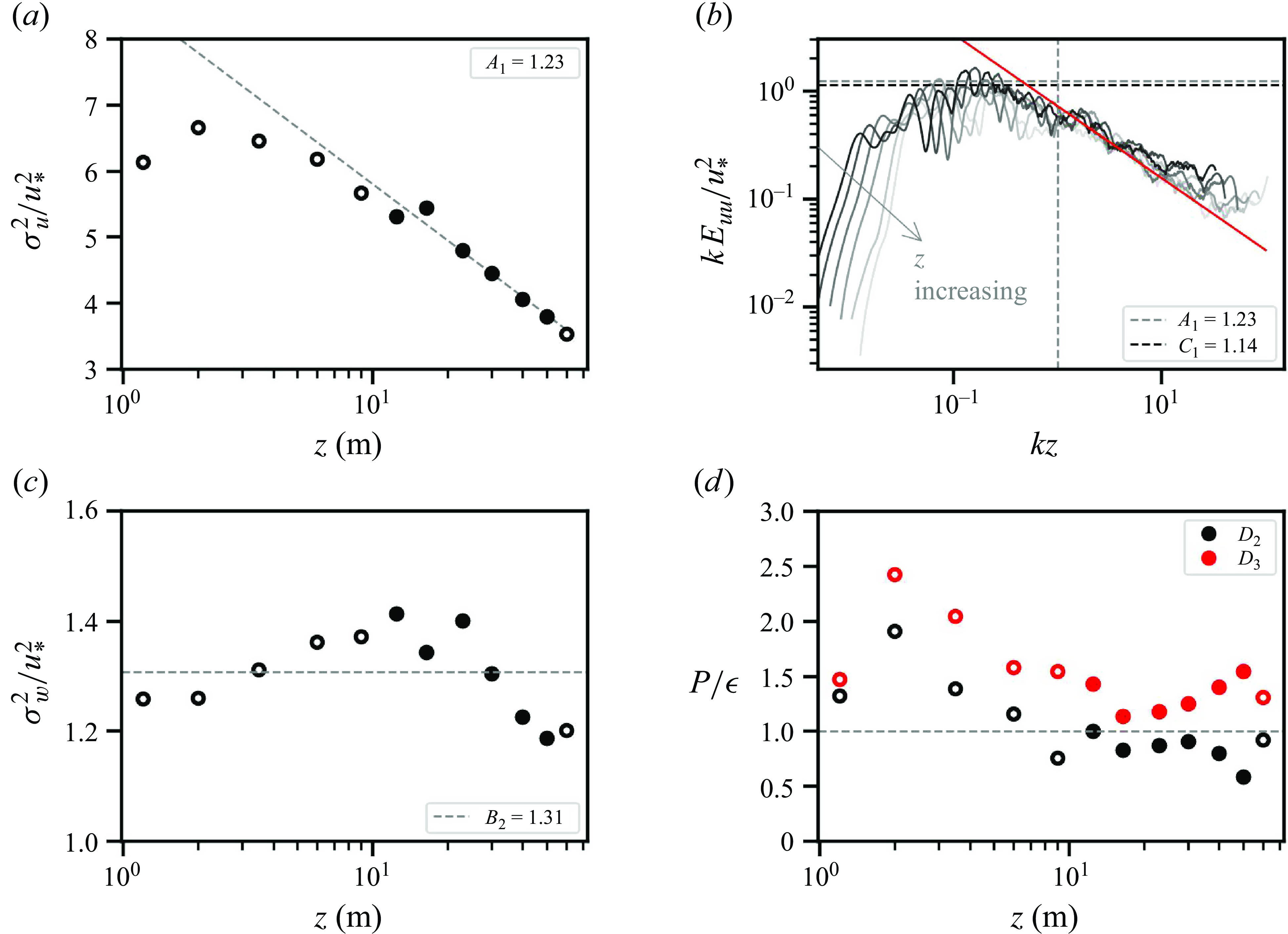
Figure 14. Example of anomalous $\sigma _w^{2}$
; similar to figure 10, with data from 14 April 2021, at 11:00 LT.
$\sigma _w^{2}$
; similar to figure 10, with data from 14 April 2021, at 11:00 LT.
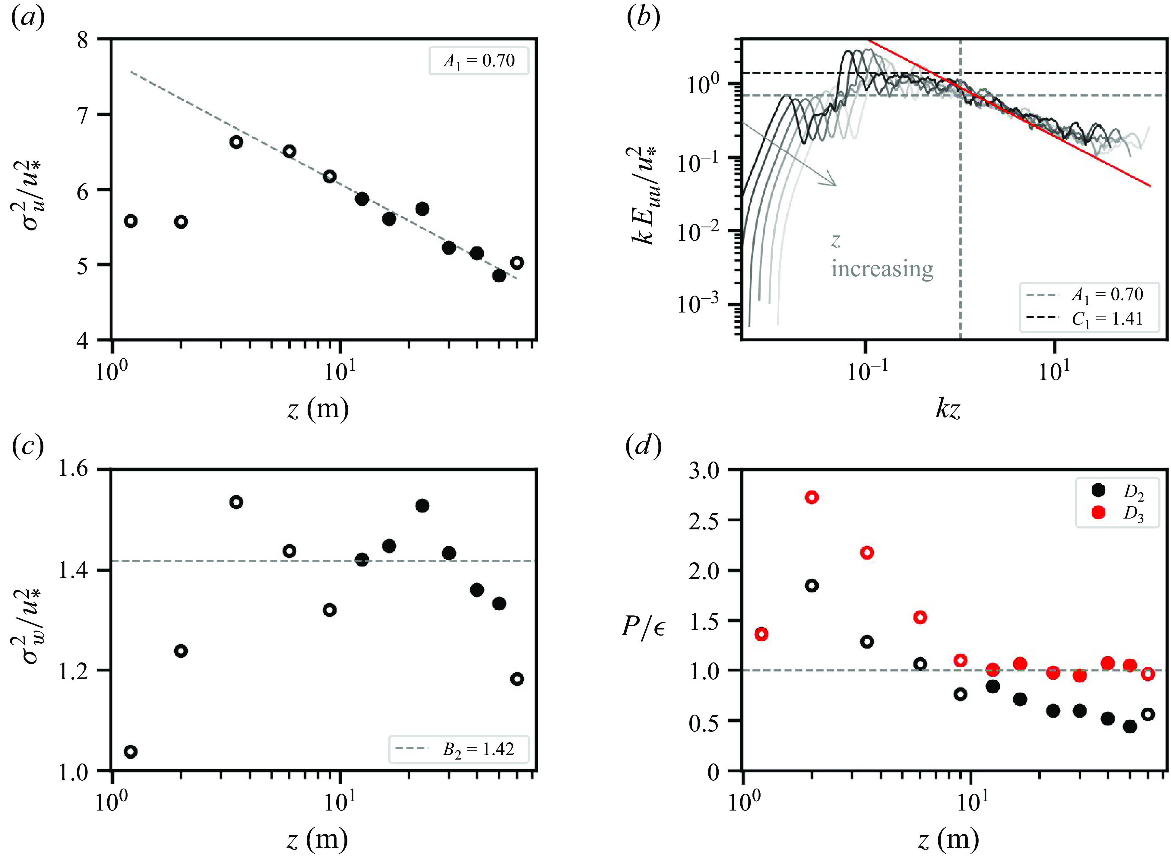
Figure 15. Example of anomalous $E_{uu}$
; similar to figure 10, with data from 10 October 2020, at 16:00 LT.
$E_{uu}$
; similar to figure 10, with data from 10 October 2020, at 16:00 LT.
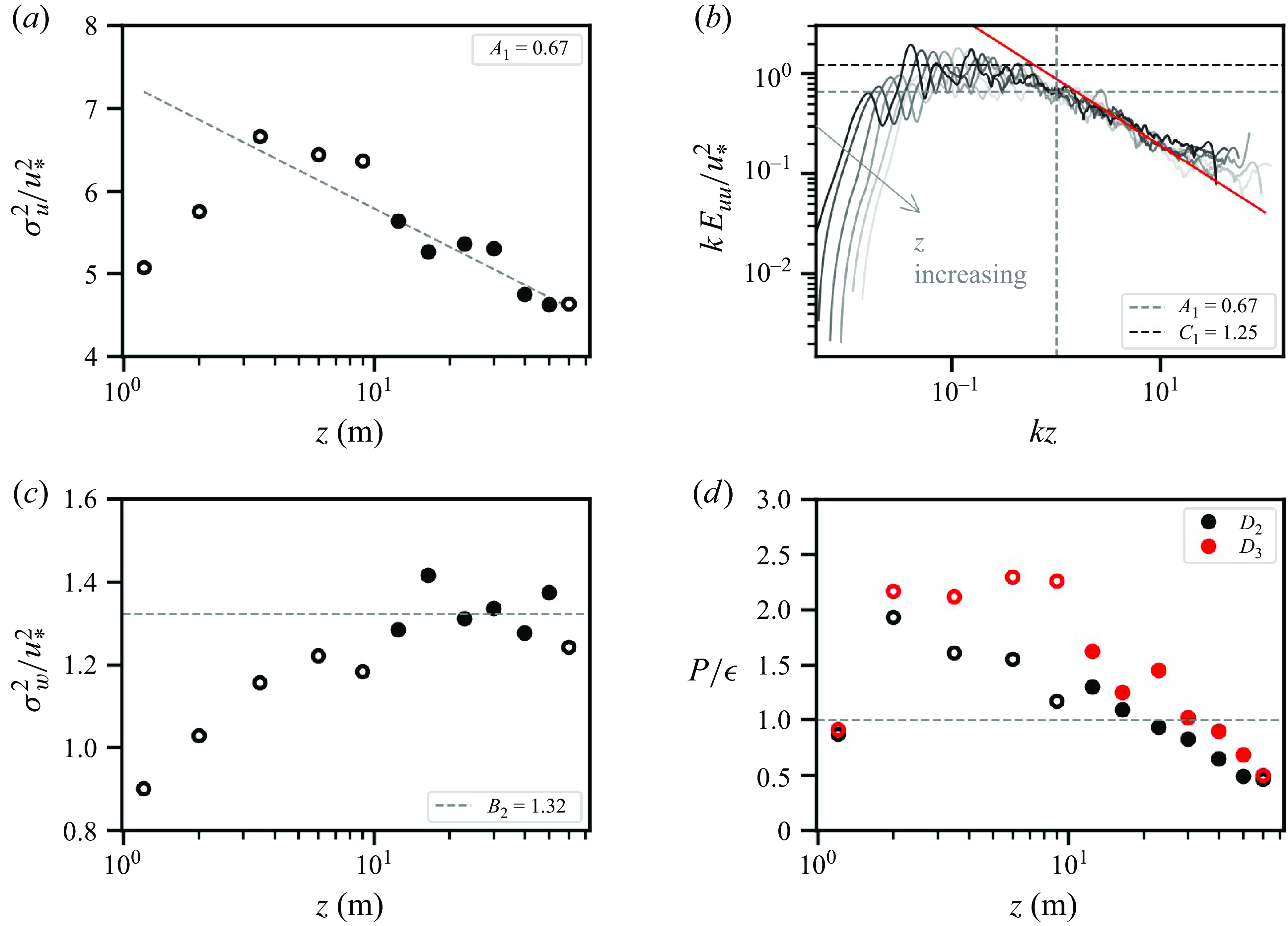
Figure 16. Example of anomalous TKE budget balance; similar to figure 10, with data from 19 November 2020, at 14:00 LT.


 Open access