


1. Introduction
Many coastal systems have topography composed of large roughness elements that is markedly different from well-studied sand grain roughness. On coral reefs and rocky coasts, for example, dominant length scales in the bottom topography can be centimetres to metres in size. Interactions of surface waves and currents with these topographies cause spatial patterns in pressure, currents, wave orbital velocities and turbulence that result in drag forces on moving water, dissipation of wave energy and mixing. In these systems, bottom friction is leading order in dynamical balances (Hench, Leichter & Monismith Reference Hench, Leichter and Monismith2008; Lowe et al. Reference Lowe, Falter, Monismith and Atkinson2009) and wave energy dissipation also affects radiation stress gradients (Monismith et al. Reference Monismith, Herdman, Ahmerkamp and Hench2013; Buckley et al. Reference Buckley, Lowe, Hansen and van Dongeron2016). Understanding combined wave and current interactions with topography composed of large roughness elements is therefore critical for predicting waves and circulation in these systems.
In systems with large roughness elements and steady flow, spatially averaged momentum and energy budgets have become a valuable tool for understanding flow over urban geometries, terrestrial forests and aquatic vegetation (as reviewed by Belcher, Harman & Finnigan (Reference Belcher, Harman and Finnigan2012) and Nepf (Reference Nepf2012)). In this approach, the Navier–Stokes equations are first time averaged, then averaged over fluid volumes thin in the vertical to resolve gradients but large in the horizontal to average over spatial variability. Spatial integration of pressure gradient and viscous terms around obstacle surfaces results in form drag and viscous drag terms in the spatially averaged momentum budget (Wilson & Shaw Reference Wilson and Shaw1977). Spatial averaging of the advective acceleration term introduces a dispersive stress, which represents momentum transport due to correlations between spatial variations in velocities within the averaging volume (Raupach & Shaw Reference Raupach and Shaw1982). The momentum balance for steady flow through obstacle arrays where obstacle layer height is substantially smaller than water depth is generally a balance between a shear stress gradient that drives the flow and form drag that opposes the flow (Nepf & Vivoni Reference Nepf and Vivoni2000). The shear stress at the top of the canopy that drives flow through the obstacle array is the same as the bottom shear stress exerted on the overlying boundary layer flow. The relative importance of turbulent (Reynolds) and dispersive stresses varies depending on array geometry; turbulent stress dominates for dense canopies in which horizontal roughness-element dimensions are small compared with canopy height (Poggi, Katul & Albertson Reference Poggi, Katul and Albertson2004), but dispersive stress is significant in sparse canopies and when horizontal roughness-element dimensions are similar to canopy height (Castro Reference Castro2017).
Less work has been done on flow over large roughness elements in coastal ocean settings, where surface waves dramatically alter boundary layer dynamics. The surface wave problem differs fundamentally from currents because boundary layer and obstacle wake development are limited by the wave period. Similar to the approach for steady flows through obstacle arrays, the Navier–Stokes equations are first phase averaged and then spatially averaged. This again results in a term that represents the force on the fluid volume due to pressure around obstacle surfaces (Lowe, Koseff & Monismith Reference Lowe, Koseff and Monismith2005; Rodriguez-Abudo & Foster Reference Rodriguez-Abudo and Foster2014; Yu, Rosman & Hench Reference Yu, Rosman and Hench2018); however, in oscillatory flows, this force has a component that is in phase with the fluid acceleration, added mass, and a component that is in phase with the velocity, form drag (Morison, Johnson & Schaaf Reference Morison, Johnson and Schaaf1950). Spatial averaging of the advective acceleration term leads to a wave dispersive stress term that is analogous to that for steady flows but varies with wave phase. In oscillatory flows over obstacle arrays, the wave dispersive stress can be as large as the oscillatory Reynolds stress (Yu et al. Reference Yu, Rosman and Hench2018).
The dynamics of oscillatory flow over an obstacle array depends on both array geometry and flow conditions. A key parameter is the Keulegan–Carpenter number (Lowe et al. Reference Lowe, Koseff and Monismith2005; Yu et al. Reference Yu, Rosman and Hench2018),  $KC=U_w T/D$, the ratio of wave orbital excursion to obstacle size multiplied by $2 {\rm \pi}$ (Keulegan & Carpenter Reference Keulegan and Carpenter1958). Here $U_w$ is the wave orbital velocity amplitude, $T$ is the wave period and $D$ is the obstacle diameter. An extensive body of work on sandy beds addresses the high $KC$ range, where orbital excursions are much larger than the obstacles and a turbulent wave boundary layer forms above the obstacle layer (e.g. Jonsson Reference Jonsson1966; Trowbridge & Madsen Reference Trowbridge and Madsen1984). In this regime, the obstacles are often thought of as surface roughness and the Reynolds stress immediately above the bed is assumed to be the same as the total force per unit area on the bottom. These models have been extended and applied in situations where $KC$ is small; however, there are fundamental differences in the dynamics at low $KC$ that these models do not capture.
A few field, laboratory and modelling studies specifically address the dynamics of wave-driven flow over obstacle arrays at lower  $KC$ (Barr et al. Reference Barr, Slinn, Pierro and Winters2004; Lowe et al. Reference Lowe, Koseff and Monismith2005, Reference Lowe, Falter, Koseff, Monismith and Atkinson2007; Nichols & Foster Reference Nichols and Foster2007; Yu et al. Reference Yu, Rosman and Hench2018). When $KC<100$, stresses above the obstacle layer are generally small compared with the total force on the bed (e.g. Sleath Reference Sleath1987; Yu et al. Reference Yu, Rosman and Hench2018). When $10< KC<100$, form drag is the dominant force exerted by the bottom on the oscillatory flow, and energy is removed from waves primarily in obstacle wakes (Lowe et al. Reference Lowe, Koseff and Monismith2005, Reference Lowe, Falter, Koseff, Monismith and Atkinson2007; Yu et al. Reference Yu, Rosman and Hench2018). Form drag due to obstacles in this parameter range can be substantially larger than the bed stress associated with the surface roughness due to sand grains (Rodriguez-Abudo & Foster Reference Rodriguez-Abudo and Foster2014). When $KC<10$, the effect of the canopy on oscillatory flow is primarily via the added-mass force, which reduces oscillatory flow in the obstacle layer. The added-mass force is in phase with the acceleration and in quadrature with the velocity; therefore, it does no work on the flow and does not result in dissipation of wave energy (Lowe et al. Reference Lowe, Koseff and Monismith2005, Reference Lowe, Falter, Koseff, Monismith and Atkinson2007). The added-mass force increases as $KC$ decreases, resulting in an apparent increase in friction factor with decreasing $KC$ when it is computed from the total force on the bed (Dixen et al. Reference Dixen, Hatipoglu, Sumer and Fredsøe2008; Yu et al. Reference Yu, Rosman and Hench2018). However, friction factors computed from only the drag force decrease as $KC$ decreases, as flow separation becomes weaker and obstacle drag coefficients decrease (Yu et al. Reference Yu, Rosman and Hench2018).
In the coastal ocean, waves and current coexist and interactions between waves and current impact dynamics and transport processes. Important parameters are the ratio of wave orbital velocity amplitude to current  $U_w/U_c$, the angle between waves and current and $KC$. Previous work on combined wave and current boundary layers has focused mainly on small-scale roughness, where $KC>O(10)$ (e.g. Soulsby et al. Reference Soulsby, Hamm, Klopman, Myrhaug, Simons and Thomas1993; Yuan & Madsen Reference Yuan and Madsen2015). In this parameter range, waves increase the time-averaged Reynolds stress near the rough bed and corresponding bottom drag on the steady flow (Umeyama Reference Umeyama2005). Waves also enhance turbulence generation at the bed, which increases the effective bottom roughness felt by the current and correspondingly the steady boundary layer thickness (Olabarrieta, Medina & Castanedo Reference Olabarrieta, Medina and Castanedo2010). Theoretical models based on simple eddy viscosity closures for turbulent stresses in the oscillatory (wave) and steady (current) boundary layers (Bakker & Van Doorn Reference Bakker and Van Doorn1978; Grant & Madsen Reference Grant and Madsen1979) have shown good agreement with laboratory experiments in this parameter range (Kemp & Simons Reference Kemp and Simons1982, Reference Kemp and Simons1983; Yuan & Madsen Reference Yuan and Madsen2015). However, these models do not represent the dynamics at lower $KC$, where the phase-averaged force per unit area acting on the flow can be different from the phase-averaged stress above the obstacle layer. Previous work on wave and current boundary layers at lower $KC$ has also observed apparent bed roughness describing the shape of the current boundary layer to be much larger than the physical roughness (Fredsøe, Andersen & Sumer Reference Fredsøe, Andersen and Sumer1999; Nayak et al. Reference Nayak, Li, Kiani and Katz2015). In this parameter range, turbulence properties vary substantially during the wave cycle as vortices are shed and interact with roughness elements (Fredsøe et al. Reference Fredsøe, Andersen and Sumer1999). The impact of these processes on the dynamics of the wave boundary layer and the energy removed from waves and current has not been fully investigated.
Interactions of flow with roughness elements are not resolved in most ocean circulation models and these subgrid-scale processes must be parametrized. Bottom friction is typically represented by a quadratic drag law with a wave friction factor for waves and a bulk drag coefficient for current. Wave friction factors,  $f_w$, are typically represented via a roughness length ( $k_s$), which is specified (e.g. Warner et al. Reference Warner, Sherwood, Signell, Harris and Arango2008). Friction factors are typically assumed to follow a single-valued function of the ratio of orbital excursion to roughness length ( $\zeta /k_s$), where the function is based on empirical relationships or theoretical curves developed for small roughness elements (e.g. Jonsson Reference Jonsson1966; Grant & Madsen Reference Grant and Madsen1979). Although applied across a broad parameter range (e.g. Lentz et al. Reference Lentz, Churchill, Davis and Farrar2016; Rogers et al. Reference Rogers, Monismith, Koweek and Dunbar2016; Rodriguez-Abudo & Foster Reference Rodriguez-Abudo and Foster2017), these curves typically assume the near-bed Reynolds stress balances the bottom drag per unit area, which is only true if roughness elements are small compared with orbital excursions (Yu et al. Reference Yu, Rosman and Hench2018). For the current, the near-bottom velocity profile is assumed to be logarithmic and bottom friction is represented via a roughness height $z_0$, which is proportional to $k_s$ (e.g. Warner et al. Reference Warner, Sherwood, Signell, Harris and Arango2008). The impact of waves on the friction felt by the current is also typically parametrized using boundary layer theory developed for small $KC$ (e.g. Grant & Madsen Reference Grant and Madsen1979). Recent observations on a coral reef suggest that bottom friction can be approximated using a quadratic drag law with combined wave and current near-bed velocities (Lentz, Churchill & Davis Reference Lentz, Churchill and Davis2018). However, the linkage between boundary layer dynamics for large roughness elements and appropriate bottom friction parametrizations is not well understood, and wave–current interactions remain among the least well-described mechanisms in most ocean wave and circulation models (Uchiyama, McWilliams & Shchepetkin Reference Uchiyama, McWilliams and Shchepetkin2010; Mellor Reference Mellor2015).
In this paper, we investigate the dynamics of combined wave–current flows over large roughness elements and implications for parametrizing bottom friction. We focus on roughness elements similar in size to wave orbital excursions,  $KC=O(1 - 10)$, an important parameter range in coastal systems like coral reefs and rocky coasts that has not been fully explored. We present a theoretical framework based on spatially and phase-averaged Navier–Stokes equations for analysing the dynamics of the steady boundary layer and the dynamics of the oscillatory flow in a combined flow. The framework is applied to results from a series of computational fluid dynamic (CFD) simulations with large-eddy simulation (LES) turbulence closure, in which important parameters were systematically varied, providing new insights into the physics of steady and oscillatory boundary layers over large roughness in combined wave–current flows. The spatial and phase averaging framework is then used to address implications for parametrization of drag on currents and dissipation of wave energy in combined flows over large roughness.
2. Background – spatial averaging framework
To investigate the dynamics of combined wave–current flow over topography, we employ a spatial and Reynolds averaging approach. The frameworks from steady (Wilson & Shaw Reference Wilson and Shaw1977) and oscillatory (Yu et al. Reference Yu, Rosman and Hench2018) flows are extended here to flows with combined currents and waves. The three velocity components and pressure are first decomposed into an ensemble average (e.g.  $\bar {u}$) and a turbulent fluctuation (e.g. $u'$). Here the phase average is used as the ensemble average. The phase-averaged streamwise velocity, for example, is defined as
 \begin{equation} {\bar{u}}(\boldsymbol{x},t) = \dfrac{\sum\limits_{n=0}^{N-1} {u}(\boldsymbol{x},t+nT)}{N}, \end{equation}
where  $T$ is the wave period, $t$ is time in the range $[0,T]$, $\boldsymbol {x}$ is position within the averaging volume and $N$ is the number of waves. The phase average is then decomposed into the spatial average, $\langle {\bar {u}}\rangle$, and the deviation from the spatial average, $\bar {{u}}''$. Spatial averaging is applied over volumes with horizontal length scales large compared with individual roughness elements but thin enough in the vertical direction to resolve the vertical structure of the flow. The intrinsic spatial average (Raupach & Shaw Reference Raupach and Shaw1982) is used, where the average is taken over the volume occupied by fluid between the bottom ( $z_1$) and top ( $z_2$) of the averaging volume:
 \begin{equation} \langle {\bar{u}}(z,t)\rangle= \dfrac{1}{V_f}\int_{z_1}^{z_2}\int_0^{L_y}\int_0^{L_x} {\bar{u}}(\boldsymbol{x},t)\,\textrm{d}V. \end{equation}
Here  $L_x$ and $L_y$ are the dimensions of the averaging volume in the horizontal directions; the spatial average is indicated by angle brackets; and $V_f$ is the volume of fluid within the averaging volume. The streamwise velocity is therefore decomposed as
 \begin{equation} {u} = \left\langle \bar{{u}}\right\rangle + \bar{{u}}'' + {u}'. \end{equation}
The same decomposition is used for the other velocity components.
The spatially averaged governing equations are derived by substituting expressions for the decomposed velocity into the Navier–Stokes equations, Reynolds (phase) averaging and then averaging each term over the fluid volume  $V_f$ (e.g. Wilson & Shaw Reference Wilson and Shaw1977; Raupach & Shaw Reference Raupach and Shaw1982; Nikora et al. Reference Nikora, McLean, Coleman, Pokrajac, McEwan, Campbell, Aberle, Clunie and Koll2007). When waves are present, it is useful to split the pressure gradient term into two parts: the oscillatory pressure gradient that drives the flow (subscript $f$) and the dynamic pressure response resulting from flow past obstacles (subscript $d$):
$d$):
 \begin{equation} \frac{\partial \bar{p}}{\partial x_i}=\frac{\partial \bar{p}_f}{\partial x_i} + \frac{\partial \bar{p}_d}{\partial x_i}. \end{equation}
The spatial averaging operator is then applied. It can be shown (see Nikora et al. Reference Nikora, McLean, Coleman, Pokrajac, McEwan, Campbell, Aberle, Clunie and Koll2007) that
 \begin{equation} \left\langle\frac{\partial \bar{p}_d}{\partial x_i}\right\rangle = \dfrac{1}{1-\phi} \dfrac{\partial (1-\phi) \langle \bar{p}_d \rangle}{\partial x_i} - \dfrac{1}{V_f}\displaystyle\int_S\bar{p}_dn_i\,\textrm{d}S. \end{equation}
The spatially averaged momentum equations can then be written as
 \begin{align} \dfrac{\partial \langle \bar{u}_i \rangle}{\partial t} + \langle \bar{u}_j \rangle \dfrac{\partial \langle \bar{u}_i \rangle}{\partial x_j} &=g_i-\dfrac{1}{\rho}\left\langle\dfrac{\partial \bar{p}_f}{\partial x_i}\right\rangle-\dfrac{1}{\rho (1-\phi)} \dfrac{\partial (1-\phi) \langle \bar{p}_d \rangle}{\partial x_i} \nonumber\\ &\quad + \dfrac{1}{\rho (1-\phi)} \dfrac{\partial (1-\phi) \tau_{ij}}{\partial x_j} -f_{Pi} - f_{Vi}, \end{align}
where
 $$\begin{gather} \tau_{ij} ={-}\rho\left\langle \overline{u'_iu'_j} \right\rangle - \rho\left\langle \bar{u}_i''\bar{u}_j''\right\rangle +\mu \dfrac{\partial \langle \bar{u}_i\rangle}{\partial x_j}, \end{gather}$$
 $$\begin{gather}f_{P_i} ={-}\dfrac{1}{\rho V_{f}}\displaystyle\int_S\bar{p}_dn_i\,\textrm{d}S, \end{gather}$$
 $$\begin{gather}f_{V_i} = \dfrac{\nu}{V_f}\displaystyle\int_S \dfrac{\partial \bar{u}_i}{\partial x_j} n_j \,\textrm{d}S. \end{gather}$$
Here,  $\phi$ is the solid volume fraction, $S$ is the solid surface, $n_i$ is the component in direction $x_i$ of the unit surface normal vector, and $\tau _{ij}$ is the sum of Reynolds stress, dispersive stress and viscous stress. The dispersive stress is the spatial analogue of the Reynolds stress and represents momentum transport due to the spatial heterogeneity of the phase-averaged flow. The pressure force term ( $f_{P_i}$) arises from expressing the spatially averaged dynamic pressure gradient in terms of the gradient of the spatially averaged dynamic pressure (2.5). The dynamic pressure field around the solid boundary exerts a force on the solid surface. There is an equal and opposite reaction force on the fluid and this is represented by $f_{P_i}$. Likewise, the viscous drag term ( $f_{V_i}$) represents the force on the fluid due to the integrated viscous stress over the solid boundary. The pressure force term is typically significantly larger than the viscous drag term; therefore, viscous drag can be neglected.
In steady flow, the pressure force  $f_{P_i}$ is equal to the form drag per unit fluid mass (e.g. Finnigan Reference Finnigan2000). In oscillatory flow, $f_{P_i}$ has an additional component due to the fluid accelerating as it moves over the solid surface (Lowe et al. Reference Lowe, Koseff and Monismith2005). Following the Morison equation (Morison et al. Reference Morison, Johnson and Schaaf1950), the total in-line force exerted on a solid body in an accelerating flow ( $U$) can be expressed as
 \begin{equation} F_x =\int_{S}\bar{p} n_x \,\textrm{d}S =\rho C_M V \dfrac{\textrm{d} U}{\textrm{d}t} + \dfrac{1}{2}\rho C_D A U\vert U \vert. \end{equation}
The first term on the right-hand side is the inertial force ( $F_I$) and the second term is the drag force ( $F_D$). The inertial force is in phase with the local flow acceleration and the drag force is in phase with the flow velocity. In the above, $V$ is the volume of the solid body, $A$ is the frontal area perpendicular to the flow direction, $C_M$ is the inertia coefficient and $C_D$ is the drag coefficient. The inertial force ( $F_I$) can be split into two terms: the added-mass force ( $F_\alpha$) and the Froude–Krylov or virtual buoyancy force ( $F_{FK}$). The Froude–Krylov force is the direct result of the unsteady pressure field that generates the oscillatory motion and is given by
 \begin{equation} F_{FK} = \int_S \bar{p}_f n_x \,\textrm{d}S=\rho V \dfrac{\textrm{d} U }{\textrm{d}t}. \end{equation}
Subtracting (2.11) from (2.10) yields
 \begin{equation} \int_S \bar{p}_d n_x \,\textrm{d}S = \rho C_\alpha V \dfrac{\textrm{d} U}{\textrm{d}t} + \dfrac{1}{2}\rho C_D A U\vert U \vert. \end{equation}
The right-hand side is the sum of the added-mass force and the drag force. The added-mass coefficient is  $C_\alpha = C_M - 1$.
The force applied on the fluid by the solid surface is equal and opposite to the force applied on the solid surface by the fluid. Dividing (2.12) by the fluid mass in the averaging volume,  $\rho V_f$, yields a parametrization for $f_{Px}$,
 \begin{equation} f_{Px} = \dfrac{C_\alpha \phi}{1-\phi}\dfrac{\textrm{d} \langle \bar{u} \rangle}{\textrm{d}t} + \dfrac{C_D A}{2V_f}\langle \bar{u}\rangle\vert \langle \bar{u} \rangle \vert , \end{equation}
where the spatially and phase-averaged velocity has been used for  $U$. The added-mass force is in phase with the local flow acceleration and in quadrature with the velocity; therefore, it does no work and does not remove energy from waves. Only the drag force, which is in phase with the flow velocity, removes energy from waves.
Although the accelerating flow also exerts a Froude–Krylov force on solid obstacles and there is a reaction force exerted on the flow, this force results from the integral around the solid surface of the pressure field that is driving the flow. The Froude–Krylov force does not appear in  $f_{Px}$ because the spatial average of the forcing pressure gradient is not split into the gradient of spatially averaged pressure and the surface integral in (2.6).
Phase-averaged quantities in the spatially averaged momentum budget are further decomposed into current and wave components. The current component, e.g.  $\langle \bar {u}_c\rangle$, is defined as the time average and the wave component is $\langle \bar {u}_w\rangle = \langle \bar {u}\rangle -\langle \bar {u}_c\rangle$. The phase-averaged streamwise velocity is therefore decomposed as
 $$\begin{gather} \langle\bar{u}\rangle = \langle \bar{u}_c \rangle + \langle \bar{u}_w \rangle , \end{gather}$$
 $$\begin{gather}\bar{u}'' = \bar{u}_c''+\bar{u}_w''. \end{gather}$$
Spanwise and vertical velocity components are decomposed in the same way. Pressure, stresses and the drag and added-mass forces are also decomposed into current and wave components in an analogous way. The governing equation for the current is then obtained by time averaging (2.6). The governing equation for the oscillatory motion is obtained by subtracting the time average from (2.6).
3. Methods
3.1. Model set-up
Numerical modelling experiments were carried out to study combined wave–current flow over a rough bottom at  $KC=2 - 12$, corresponding to wave orbital excursions ranging from ${1}/{3}$ to $2$ times the obstacle diameter. The bottom was an infinite two-dimensional array of regularly spaced hemispheres on a flat horizontal surface (figure 1). Hemisphere dimensions and spacing were based on field measurements on a reef flat in Moorea, French Polynesia, reported by Hench & Rosman (Reference Hench and Rosman2013) and Duvall et al. (Reference Duvall, Rosman and Hench2020). For the main set of simulations, the hemisphere diameter $D$ was 0.5 m, the centre-to-centre spacing $S$ was 1 m and the height $H$ of the domain (i.e. water depth) was 2 m. The horizontal dimensions of the simulation domain were equal to the distance between the centres of adjacent hemispheres ( $S$). Periodic boundary conditions were applied in both horizontal directions, a free-slip boundary condition was applied at the top, and a smooth-wall boundary condition was applied at the bottom, including the surface of the hemisphere.

Figure 1. Schematic diagram showing the hemisphere array, simulation domain and boundary conditions.
To assess potential effects of domain size, we carried out one simulation with a larger domain (2 $S$ in the flow direction and two hemispheres in the domain). While there were some differences in the steady boundary layer in the upper half of the domain, the drag force and phase-averaged velocities agreed well with the baseline simulation, with differences less than 3 %. Phase-averaged turbulent and dispersive stresses above the top of the canopy differed by about 10 % of the peak stresses, most likely because these higher-order statistics were more fully converged when the averaging volume was larger. Turbulence decorrelation length scales at $z/D=1$ were about 20 % of the domain size. These analyses indicate that turbulence length scales larger than the domain do not have a major role in the physics in the roughness sublayer and the domain size is not expected to affect our conclusions. To assess the importance of flow sheltering between adjacent hemispheres, two additional simulations with $S = 0.75~\textrm {m}$ were conducted. While the drag was slightly decreased due to flow sheltering for the more closely spaced hemispheres, the effect was minor and did not affect our conclusions, so these simulations are not discussed further.
The computational grid was generated using utilities in the OpenFOAM package (Weller et al. Reference Weller, Tabor, Jasak and Fureby1998). A block structured grid with finer cells near the hemisphere surface was used. The blockMesh utility was used to generate the grid and the mesh was fitted to the hemisphere surface using the blockMeshBodyFit tool. The smallest grid cells were 2.6 mm and the total number of grid cells was  $5.68 \times 10^6$. A fixed time step was chosen for each case such that a Courant number less than unity was maintained.
To obtain initial conditions for the combined wave and current simulations, we first ran a simulation with current only. Steady-state velocity and turbulence fields from those simulations were used to initialize simulations with combined waves and current. Simulations with combined waves and current reached a fully developed state, in which flow properties were stationary, in 50 wave cycles. Therefore, the first 50 wave cycles of each simulation were deemed ‘spin-up’ and not used in the analysis. After spin-up, the number of wave cycles used to compute flow and turbulence statistics was systematically increased to determine the number of wave cycles needed for the phase-averaged flow and turbulence statistics to converge. Although it was not feasible to continue simulations long enough that time-averaged stress profiles were perfectly smooth, there were no meaningful changes in quantities of interest after 40–50 wave cycles. Therefore,  $N=50$ wave cycles was used to calculate all phase averages. Simulations were run on high-performance computer clusters at the University of North Carolina at Chapel Hill and the University of Florida. Each simulation with current alone required about 25 000 CPU hours and each simulation with waves required an additional 40 000 CPU hours.
3.2. Large-eddy simulation model
Simulations were conducted using OpenFOAM (version 3.0; Weller et al. Reference Weller, Tabor, Jasak and Fureby1998). The current was driven by a constant pressure gradient term  $f_{c}$. Oscillatory motion was driven by an oscillating (sinusoidal) horizontal pressure gradient, representing near-bottom flow under small-amplitude waves in shallow or intermediate water depths. Sufficiently high above the hemispheres, the momentum equation describing the oscillating part of the flow reduces to
 \begin{equation} \dfrac{\partial u_{w,\infty}}{\partial t} ={-}\dfrac{1}{\rho} \dfrac{\partial p_w}{\partial x}. \end{equation}
A sinusoidal free-stream velocity was used with  $u_{w,\infty } = U_w\sin (\omega t)$, where $U_w$ is the amplitude of the oscillating free-stream velocity. The pressure gradient driving the combined flow was therefore $-\textrm {d}p_\infty /{\textrm {d} x}=\rho U_w\omega \cos (\omega t)+\rho f_c$. Hence, the governing equations can be written as
 $$\begin{gather} \dfrac{\partial u_i}{\partial x_i} = 0, \end{gather}$$
 $$\begin{gather}\dfrac{\partial u_i}{\partial t}+\dfrac{\partial u_i u_j}{\partial x_j} ={-}\dfrac{1}{\rho}\dfrac{\partial p_d}{\partial x_i} + \dfrac{1}{\rho}\dfrac{\partial \tau_{ij}}{\partial x_j}+U_w \delta_{i1}\omega \cos(\omega t) +f_c\delta_{i1}, \end{gather}$$
where  $u_i$ is the resolved fluid velocity, $p_d$ is the dynamic pressure, $\rho$ is the density of the fluid, $\tau _{ij}$ is the stress term, including both the turbulent stress and viscous stress components, and $\delta$ is the Kronecker delta. The total pressure is $p=p_d+(x-x_0)\,{\textrm {d}p_\infty }/{\textrm {d} x}$, where $x_0$ is a reference position at which pressure is defined to be zero.
LES turbulence closure was used to calculate the turbulent stresses. In LES, large-scale turbulent motions are resolved and the turbulent stress term represents only momentum fluxes by small-scale processes not adequately resolved on the computational grid. LES has been successfully applied to study flow over complex topography in many engineering applications (Barr et al. Reference Barr, Slinn, Pierro and Winters2004; Xie & Castro Reference Xie and Castro2009; Anderson et al. Reference Anderson, Passalacqua, Porté-Agel and Meneveau2012; Chakrabarti et al. Reference Chakrabarti, Chen, Smith and Liu2016). Unlike other turbulence models, LES captures interactions between turbulent wakes and roughness elements, which is important for mass and momentum transfer in the canopy and roughness sublayers of rough boundary layers.
The wall-adapting local eddy viscosity (WALE) model (Ducros, Nicoud & Poinsot Reference Ducros, Nicoud and Poinsot1998) was used as the subgrid closure. In the WALE model, the stress term is
 \begin{equation} \tau_{ij} = 2(\nu_t +\nu)S_{ij}, \end{equation}
where  $S_{ij}$ is the strain-rate tensor of the resolved scale, $\nu$ is the kinematic viscosity of the fluid and the eddy viscosity $\nu _t$ is given by
 \begin{equation} \nu_t = \varDelta_s^2 \dfrac{(S_{ij}^dS_{ij}^d)^{3/2}} {(S_{ij}S_{ij})^{5/2}+(S_{ij}^dS_{ij}^d)^{5/4}} , \end{equation}
with
 $$\begin{gather} \varDelta_s = C_wV_c^{1/3}, \end{gather}$$
 $$\begin{gather}S_{ij}^d=\tfrac{1}{2}(g_{ij}^2+g_{ji}^2)-\tfrac{1}{3}\delta_{ij}g_{kk}^2, \end{gather}$$
 $$\begin{gather}g_{ij} = \dfrac{\partial u_i}{\partial x_j}. \end{gather}$$
The constant  $C_w = 0.325$ and $V_c$ is the volume of the grid cell. While the WALE model can be overdissipative in strong vortical flows (Bricteux, Duponcheel & Winckelmans Reference Bricteux, Duponcheel and Winckelmans2009), it has been found to perform better than the dynamic Smagorinsky model for simulating flow separation (Arya & De Reference Arya and De2019) and flow over rough beds (Lian et al. Reference Lian, Dallmann, Sonin, Roche, Liu, Packman and Wagner2019). For this study, the main turbulent generation mechanism is eddies shed from the roughness elements and no strong shear layers formed; therefore, the WALE model is appropriate.
3.3. Simulations conducted
A series of 10 simulations with different parameter combinations were carried out (table 1). We used two current forcings,  $f_c$, which are referred to as weak current (cases 1 to 5) and strong current (cases 6 to 10). For a given $f_c$, the resulting current varied somewhat depending on wave properties. Both the depth-averaged current through the entire water column ( $U_{c,H}$) and the depth-averaged current within the canopy layer ( $U_{c}$) are reported in table 1. The dynamics is dominated by the interaction of the flow with the hemispheres; therefore, the spatially averaged velocity in the canopy layer, the layer containing solid obstacles, is used as the characteristic current velocity $U_c$. The two key dimensionless parameters, i.e. the ratio of wave orbital velocity to current ( $U_w/U_c$) and the Keulegan–Carpenter number ( $KC=U_w T/D$), were varied by changing the free-stream wave velocity amplitude ( $U_w$) and wave period ( $T$) for each current forcing. The Stokes number ( $\beta =D^2/\nu T$) is the squared ratio of the characteristic length scale of bottom topography to the laminar wave boundary layer thickness and was $O(10^4)$ for all simulations. The dependence of flow characteristics on $\beta$ was therefore weak and is not a focus of the analyses.
Table 1. Summary of simulation parameters.

4. Results
4.1. Flow kinematics
Depending on the relative strengths of the current and wave velocities, the mean flow may or may not change directions in the canopy layer during a wave cycle, resulting in different flow behaviour. Two contrasting cases are used to illustrate flow features for cases with different  $U_w/U_c$: a representative wave-dominated case with weak current forcing and $U_w = 0.3\ \textrm {m}\ \textrm {s}^{-1}$ ( $U_w/U_c = 8.6$, $KC = 12$; case 4); and a representative current-dominated case with strong current forcing and $U_w = 0.1\ \textrm {m}\ \textrm {s}^{-1}$ ( $U_w/U_c = 0.7$,
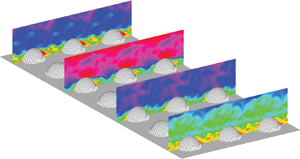
  $KC = 4$; case 7). For the wave-dominated case, there is weak flow separation, and the pressure fields under the wave peak (figure 2b,f) and wave trough (figure 2d,h) have similar small-scale fluctuations in the wake zones. However, due to the current, turbulence is slightly stronger at $\omega t = {\rm \pi}$ (decelerating) than at $\omega t = 0$ (accelerating). For the current-dominated case, $U_w/U_c$ is smaller than unity and the flow does not change direction even under the wave trough (figure 2i–p). During the part of the wave cycle when the velocity increases ( $\omega t$ from 0 to ${\rm \pi} /2$), the wake zone grows, flow separation is strong and more small-scale pressure fluctuations form (figure 2j). Because the flow does not reverse, the wake behind the hemisphere continues to grow, and eddies generated in the wake of adjacent hemispheres interact with the local hemisphere (figure 2k,o). At $\omega t=3{\rm \pi} /2$ (figure 2l,p), small-scale fluctuations can be seen all across the plane.

Figure 2. Example pressure and velocity fields from the LES at four different wave phases for: (a–h) a case with weak current and strong waves (case 4:  $U_{c,H} = 0.14\ \textrm {m}\ \textrm {s}^{-1}$, $U_w = 0.3\ \textrm {m}\ \textrm {s}^{-1}$, $T = 20\ \textrm {s}$); and (i–p) a case with strong current and weak waves (case 7: $U_{c,H} = 0.30\ \textrm {m}\ \textrm {s}^{-1}$, $U_w = 0.1\ \textrm {m}/$, $T = 20\ \textrm {s}$). Colours are dynamic pressure $p_d/\rho$ normalized by mean-squared velocity and vectors are velocity fields. The $x$–
$x$– $z$ plane is located in the centre of the domain and the $x$–
$x$– $y$ plane is located at $z/D = 0.2$.
Spatially averaged velocity profiles generally have two distinct parts (figure 3). Above  $z/D = 0.5$ the velocity profile has the shape of a characteristic steady boundary layer with a vertically uniform oscillatory velocity superposed. Inside the canopy layer, the velocity profile is affected by the flow structure around the hemispheres. Dissipation rates are generally small in the boundary layer above the hemispheres and much larger in the canopy layer, due to turbulence generated in hemisphere wakes. Dissipation rates are higher for cases with larger waves and highest when flow is decelerating, between the peak and trough when the flow excursion is greatest and the wake is longest. In the decelerating part of the wave cycle, some dissipation occurs above the hemispheres up to $z/D=1$ for cases with large waves, indicating that some turbulence is transported upwards into the water column above the canopy layer as the flow reverses (figure 3g,o). However, in all cases, most of the dissipation occurs in obstacle wakes within the canopy layer.

Figure 3. Phase- and spatially averaged (a–d) velocity and (e–h) dissipation rate profiles at four different wave phases for simulations with weak current and different wave velocity amplitudes and wave periods (cases 2–5). (i–p) Equivalent velocity and dissipation rate profiles for the strong current simulations (cases 7–10).
Waves have a more dramatic effect on velocity profile shapes and dissipation rates for cases with weak current than for cases with strong current. For weak current cases, dissipation rates are much higher in the canopy layer for cases with larger waves. At  $\omega t = 0$ and $\omega t = {\rm \pi}$ (figure 3a,c), velocity profiles from cases with small $KC = 4$ (case 2: $U_w = 0.1\ \textrm {m}\ \textrm {s}^{-1}$, $T = 20\ \textrm {s}$; and case 5: $U_w = 0.2\ \textrm {m}\ \textrm {s}^{-1}$, $T = 10\ \textrm {s}$) are similar to the steady current profile. However, velocity profiles from cases with larger $KC$ deviate from the steady current case because of the stronger turbulent mixing and dissipation. For cases with strong current, the normalized velocity profile shape only differs significantly from other profiles for the case with strongest waves (case 9: $U_w = 0.3\ \textrm {m}\ \textrm {s}^{-1}$, $T = 20\ \textrm {s}$) and the impact of waves on dissipation rates is less strong (figure 3i,p).
4.2. Drag and inertial forces
The primary influence of the hemispheres on the spatially averaged momentum balance is from forces exerted on water in the canopy layer due to the pressure field around the hemispheres. This force is equal and opposite to the force exerted by the fluid on the hemispheres. The total in-line force acting on the hemisphere in the streamwise direction was computed from the simulated pressure field as
 \begin{equation} F_x=\int_S p n_x \,\textrm{d}S = \int_S p_d n_x \,\textrm{d}S + \rho V_{hem} \dfrac{\textrm{d}u_{w,\infty}}{\textrm{d}t} + \rho V_{hem} f_c, \end{equation}
where  $n_x$ is the streamwise component of the unit normal vector and $V_{hem} = \tfrac {1}{12}{\rm \pi} D^3$ is the volume of the hemisphere. The second term on the right-hand side of (4.1) is the Froude–Krylov force caused by the unsteady pressure gradient that drives the flow. The last term represents the force due to the pressure gradient that drives the current.
The in-line force  $F_x$ was parametrized using Morison's equation (2.10). The instantaneous phase-averaged velocity was approximated as $\langle \bar {u}(t) \rangle = U_c + U_w \sin (\omega t)$, where $U_c$ is the depth-averaged current in the canopy layer and $U_w$ is the amplitude of the wave component of velocity. Morison's equation can then be written as
 \begin{equation} F_x = \dfrac{1}{2} \rho \alpha C_D A_{hem} (U_c + U_w\sin \omega t) \vert U_c + U_w \sin \omega t\vert + \rho C_M V_{hem} \dfrac{\textrm{d} \langle \bar{u} \rangle}{\textrm{d}t}. \end{equation}
The coefficient  $\alpha$ arises because of the way $C_D$ is defined. We define $C_D$ using the root-mean-square (r.m.s.) drag force and the r.m.s. spatially averaged velocity in the canopy layer:
 \begin{equation} C_D=\dfrac{F_{D,rms}}{\tfrac{1}{2}\rho A_{hem} (u_{rms})^2}. \end{equation}
The r.m.s. of the velocity squared, which appears in the quadratic drag parametrization, is  $(u^2)_{rms}=(U_c^4+3U_c^2U_w^2+\frac {3}{8}U_w^4)^{1/2}$, while the square of the r.m.s. velocity in the $C_D$ definition is $(u_{rms})^2 = U_c^2+\frac {1}{2}U_w^2$. The coefficient $\alpha$ is the ratio of these quantities, which can be written in terms of $U_w/U_c$ as
 \begin{equation} \alpha = \dfrac{(u_{rms})^2}{(u^2)_{rms}} = \dfrac{1+\dfrac{1}{2}\left(\dfrac{U_w}{U_c}\right)^2} {\,\sqrt{1+3\left(\dfrac{U_w}{U_c}\right)^2+ \dfrac{3}{8}\left(\dfrac{U_w}{U_c}\right)^4}\,}. \end{equation}
The drag and inertial forces and the force coefficients in (4.2) were obtained using a least-squares method, given  $F_x$, $U_c$, $U_w$ and $\textrm {d} \langle \bar {u} \rangle /\textrm {d}t$ from the simulations.
The quantity  $C_D\alpha$ varies by approximately a factor of 2 among all simulations with combined waves and current and has clear patterns with $U_w/U_c$ and $KC$ (figure 4). Generally, when $U_w/U_c$ is small (current-dominated cases), $C_D\alpha$ is high and there is little dependence on $KC$ but a strong dependence on $U_w/U_c$. When $U_w/U_c$ is large (wave-dominated cases), $C_D\alpha$ varies less with $U_w/U_c$ but increases strongly with $KC$, as orbital excursion increases and flow separation is more developed. At large $U_w/U_c$, $C_D\alpha$ converges to values for oscillatory flow simulations with no current from Yu et al. (Reference Yu, Rosman and Hench2018). The $C_D\alpha$ value decreases as wave velocity increases relative to current (increasing $U_w/U_c$) because flow separation is less developed and wakes are weaker in oscillating flows than in steady flows with similar r.m.s. velocities. For the same value of $U_w/U_c$, $C_D\alpha$ increases with $KC$, due to stronger flow separation and the $KC$ dependence becomes stronger as $U_w/U_c$ increases.

Figure 4. Drag parameter  $C_D \alpha$ versus ratio of wave orbital velocity to current in the canopy layer ( $U_w/U_{c}$) and Keulegan–Carpenter number ( $KC$). In (a,b), red diamonds are simulations with strong current (cases 6–10), blue circles are simulations with weak current (cases 1–5), and black triangles are simulations with no current from Yu et al. (Reference Yu, Rosman and Hench2018). In (c), diamonds are strong current cases, circles are weak current cases, and lines are contours of $C_D \alpha$; points and contours are coloured according to $C_D \alpha$.
To examine the variation of the drag force over a wave cycle, and compare it with quadratic drag law predictions, normalized drag force is plotted as a function of wave phase in figure 5. For simulations with small  $U_w/U_c$, flow direction does not strongly reverse during the wave cycle and in most cases the drag force shows a sharply peaked crest and a flat trough that are captured by the quadratic drag relationship. However, the drag force at the wave trough is underpredicted by the quadratic drag law for these cases. For cases with large $U_w/U_c$, the drag force is more symmetric between the positive and negative half-cycles of the wave, and this is also captured by the quadratic drag relationship. Generally, the variation in drag force over the wave cycle is captured well by the quadratic drag parametrization for simulations with high $KC$. Agreement with the quadratic drag relation is poorer for low $KC$ cases, probably because the wave period ( $T$) is short compared with the time scale for development of flow separation, which scales with $D/U_w$, so the wake and the pressure field around the hemisphere do not develop fully and adjust to the incident velocity throughout the wave cycle.

Figure 5. Drag force on a hemisphere as a function of wave phase for (a,c) weak current cases 2–5 and (b,d) strong current cases 7–10. (a,b) Drag force calculated from phase average of simulated pressure field, normalized using the mean-square spatially averaged velocity in the canopy layer. (c,d) Drag force predicted by a quadratic drag law and sinusoidal velocity in the canopy layer:  $\mathcal {U}=U_{c}+U_w\sin {\omega t}$, where $U_{c}$, $U_w$ and $C_D\alpha$ were set to values from each simulation.
4.3. Effects of waves on current
To investigate how waves affect the current, we consider the spatially averaged and phase-averaged momentum equations from (2.6). The spatial averaging volume is taken as a thin slab with horizontal dimensions equal to the centre-to-centre spacing between hemispheres. Because the domain is periodic in the horizontal ( $x$ and $y$) directions, horizontal gradients of the spatially averaged velocity components and stresses are zero. The spatially averaged vertical and lateral velocity components, $\langle \bar {w} \rangle$ and $\langle \bar {v} \rangle$, are zero following the continuity equation and boundary conditions. The pressure gradient driving the current is $f_c$ and the pressure gradient driving the oscillatory flow is $U_w \omega \cos (\omega t)$. The double-averaged momentum equation in the flow ( $x$) direction can therefore be simplified as
 \begin{equation} \frac{\partial \langle \bar{u} \rangle}{\partial t} = f_c+U_w \omega \cos \omega t - f_{P} + \frac {1}{\rho}\frac{\partial \tau_{xz}}{\partial z}, \end{equation}
where  $f_{P}$ represents the sum of drag and added-mass forces, and $\tau _{xz}$ is the sum of the spatially averaged Reynolds stress, dispersive stress and viscous stress terms. The viscous stress is negligible; therefore, $\tau _{xz} = \tau _{xz}^{turb}+\tau _{xz}^{disp}=-\rho \langle \overline {u'w'}\rangle -\rho \langle \bar {u}''\bar {w}'' \rangle$. To investigate wave effects on currents, (4.5) is time-averaged over the wave cycle, which gives
 \begin{equation} f_c - f_{D,c} + \frac{1}{\rho} \frac{\partial \tau_{xz,c}}{\partial z} = 0. \end{equation}
The subscript  $c$ represents the current component.
While Reynolds stress is the dominant stress component in the steady boundary layer above the hemispheres, dispersive stress is significant for vertical momentum transfer within the canopy (figure 6). For both weak and strong current cases, the dispersive stress peaks within the canopy layer and drops to zero quickly above the canopy. The non-zero dispersive stress much further away from the canopy layer in some cases is probably due to insufficient data to obtain good statistics. The dispersive stress increases with wave velocity and is more important for the weak current cases, for which waves dominate. For the weak current case with  $KC = 12$ (case 4), the peak dispersive stress is almost 60 % of the peak Reynolds stress (figure 6a). Other than case 7 ( $KC = 4$ with strong current), the time-averaged dispersive stress has the same sign as the Reynolds stress, indicating downward transport of faster-moving fluid (figure 6b). Above the top of the canopy layer, Reynolds stresses are consistent with the theoretical linear profile obtained when the drag force ( $f_{D,c}$) in (4.6) is zero. The enhanced peak in Reynolds stress near the top of the canopy layer ( $z/D = 0.5$) for more current-dominated cases is probably the result of stronger shear at the top of the canopy in those cases.

Figure 6. Time-averaged stress profiles. Three cases with different wave orbital amplitudes ( $U_w = 0.1\ \textrm {m}\ \textrm {s}^{-1}$, $0.2\ \textrm {m}\ \textrm {s}^{-1}$, $0.3\ \textrm {m}\ \textrm {s}^{-1}$) and the same wave period ( $T = 20\ \textrm {s}$) are shown for (a) weak current (cases 2–4) and (b) strong current (cases 7–9). Solid lines indicate turbulent stresses $\langle \overline {u'w'}\rangle _c$ and dashed lines indicate dispersive stresses $\langle \bar {u}'' \bar {w}'' \rangle _c$. Stresses are normalized by $\tau _c$, the force per unit horizontal area that must be exerted by the bottom on the fluid to balance the pressure gradient imposed to drive the current. The grey shaded region indicates the canopy layer.
The shear stress drives the current in the canopy layer and opposes the current in the water column above the hemispheres, although the relative importance of Reynolds stress and dispersive stress varies with wave conditions (figure 7). Above the canopy, the pressure gradient driving the flow is balanced by the shear stress gradient, which acts to decelerate the flow. In the canopy layer, the shear stress gradient, which acts to accelerate the flow, is balanced mostly by the drag force, and the pressure gradient imposed to drive the current ( $f_c$) is small by comparison. As $U_w/U_c$ increases, the dispersive stress gradient becomes progressively more important relative to the Reynolds stress gradient for driving the current in the canopy layer. For case 4 with strong waves and weak current ( $KC = 12$, $U_w/U_c=8.4$), the dispersive stress gradient is similar in size to the Reynolds stress gradient (figure 7a). For case 7 with weak waves and strong current ( $KC = 4$, $U_w/U_c = 0.7$), the dispersive stress is less important (figure 7b). However, near the top of the canopy layer, where the drag force is small, the dispersive stress gradient balances the Reynolds stress gradient. This suggests that, even when waves are weak relative to the current, the dispersive stress is important in the vertical momentum transfer at the top of the canopy layer.

Figure 7. Profiles of terms in the time- and spatially averaged momentum budget for (a) weak current and strong waves (case 4:  $U_w/U_{c} = 8.36$, $KC = 12$), and (b) strong current and weak waves (case 7: $U_w/U_{c} = 0.70$, $KC = 4$). Momentum budget terms are normalized by $f_c$, the pressure gradient force imposed to drive the current. The grey shaded region indicates the canopy layer.
We now examine how the net frictional force per unit bottom area ( $\rho u_*^2$) varies among cases with different wave and current conditions. In the depth-integrated time-averaged momentum balance for the entire water column, the pressure gradient that drives the flow is balanced by the total bottom friction that opposes the flow. The friction velocity can therefore be calculated from $u_* = \sqrt {f_c H_{eff}}$, where $H_{eff}$ is the effective water depth, equal to the total volume of water in the domain divided by the plan area. While $u_*$ is the same for all simulations with the same $f_c$, the currents that develop in response to the imposed $f_c$ differ. The normalized friction velocity $u_*/U_{c}$ increases with the ratio of wave velocity to current in the canopy layer (figure 8b). The effect of waves on $u_*/U_c$ can be predicted using a quadratic drag parametrization together with a sinusoidal velocity $U_c+U_w \sin (\omega t)$ in the canopy layer. This yields
 \begin{equation} u_*^2=\frac{F_{D,c}}{\rho S^2} =\frac{1}{\rm \pi}C_D\alpha \lambda_F U_c^2 \left( \left[1 + \frac{1}{2} \left(\frac{U_w}{U_c} \right)^2 \right] \arcsin{\frac{U_c}{U_w}} + \frac{3}{2} \sqrt{\left(\frac{U_w}{U_c}\right)^2-1} \right). \end{equation}
Here  $F_{D,c}$ is the time-averaged drag force on the hemisphere, $S$ is hemisphere spacing and $\lambda _F={\rm \pi} D^2/8 S^2$ is frontal area per unit plan bottom area in the array. Generally, friction velocities calculated from the simulations agree well with quadratic drag law predictions, although the quadratic model slightly underpredicts $u_*$ for wave-dominated cases (figure 8b).

Figure 8. Normalized friction velocity,  $u_*/U_{c}$, and zero-plane displacement, $d/D$, versus (a,c) $KC$ and (b,d) $U_w/U_{c}$. Red diamonds indicate simulations with weak current (cases 1–5) and blue circles indicate simulations with strong current (cases 6–10). Dotted lines in (b) are quadratic drag law predictions (4.7) with three different $C_D \alpha$ values.
Waves are also expected to enhance vertical mixing and momentum exchange between the canopy layer and the overlying water column. One indicator of vertical momentum transfer is the mean height of momentum absorption in the canopy layer. This represents the average position of the momentum sink (drag) in the canopy, or equivalently the depth to which the shear stress gradient driving flow through the canopy penetrates into the canopy. The displacement  $d$ was calculated following
 \begin{equation} d = \dfrac{\displaystyle\int_0^{D/2} \dfrac{\partial \tau_{xz,c}}{\partial z}z\,\textrm{d}z}{\displaystyle\int_0^{D/2} \dfrac{\partial \tau_{xz,c}}{\partial z}\,\textrm{d}z}. \end{equation}
In our study,  $d$ varies with both $KC$ and $U_w/U_c$ (figure 8c,d). The displacement $d$ is often written as $d = k h$, where $h$ is the height of the physical roughness element. At small $KC$ and $U_w/U_c$ (current-dominated), $d/D$ is around 0.3 for both the strong and weak current cases, which gives the value $k = 0.6$. When the wave velocity is larger than the current velocity, $U_w/U_c>1$, and the wave orbital excursion is substantial relative to the hemisphere diameter ( $KC>3$), $d/D$ is much smaller, around 0.05 to 0.1 ( $k = 0.1$ to 0.2). The relatively small values of $k$ in our study are probably due to the relatively sparse configuration of roughness elements. The zero-plane displacement $d$ decreases with $U_w/U_c$ for cases with the same $KC$ (figure 8d), because waves enhance vertical momentum transport by turbulence and dispersion in the canopy layer.
When roughness elements are small relative to the water depth, there is a portion of the boundary layer where turbulence is not affected by either the roughness elements or the water depth, resulting in a logarithmic velocity profile shape. The velocity profile in the logarithmic layer is typically written (Jackson Reference Jackson1981) as
 \begin{equation} u_c = \dfrac{u_*}{\kappa}\ln\dfrac{(z-d)}{z_0}, \end{equation}
where  $u_c$ is the current velocity at height $z$ above the bottom and $\kappa$ is the von Kármán constant. In this study, although the mean velocity profile appeared to be logarithmic over part of the water depth, the slope differed significantly from $u_*/\kappa$. This occurred because roughness-element height was a significant fraction of the water depth (0.125) and therefore no region existed in which turbulence was not affected by processes at the boundary or constrained by the water depth. For this reason, we do not report estimates for $u_*$, $d$ or $z_0$ from logarithmic fits to velocity profiles.
4.4. Effects of current on waves
To investigate how the current affects the waves, we used the phase-varying part of the spatially and phase-averaged momentum equations in (2.6). The momentum equation for the wave component is derived by subtracting (4.6) from (4.5), which yields
 \begin{equation} \dfrac{\partial(\langle \bar{u}\rangle_w - u_{w,\infty})}{\partial t} ={-}f_{P,w}+\frac{1}{\rho}\dfrac{\partial \tau_{xz,w}}{\partial z}. \end{equation}
Here  $u_{w,\infty }=U_w \sin (\omega t)$ is the oscillating part of the free-stream velocity and $f_{P,w}$ is the oscillating part of the force on the fluid from the pressure field around the hemisphere (drag and added-mass forces). The oscillating shear stress includes Reynolds stress and dispersive stress components, $\tau _{xz,w} = \rho (-\langle \overline {u'w'}\rangle _w - \langle \bar {u}_c''\bar {w}_w'' \rangle -\langle \bar {u}_w''\bar {w}_c'' \rangle -\langle \bar {u}_w''\bar {w}_w''\rangle _w$). The wave components of the stress terms are calculated as $\langle \overline {u'w'}\rangle _w = \langle \overline {u'w'}\rangle -\langle \overline {u'w'}\rangle _c$, $\langle \bar {u}_w''\bar {w}_w''\rangle _w=\langle \bar {u}_w''\bar {w}_w''\rangle -\langle \bar {u}_w''\bar {w}_w''\rangle _c$, in which the subscript $c$ means time average.
As indicated previously, the dispersive stress can be important in the dynamics when waves are present. To examine the relative contributions of the dispersive stress components and their variation through the wave cycle, figure 9 shows the decomposition of the dispersive stress term for a wave-dominated case and a current-dominated case. For the weak current (wave-dominated) case, the oscillatory dispersive stress (figure 9a) is much larger than the time-averaged dispersive stress (figure 9e). The spatial correlation between oscillating horizontal and vertical velocity components,  $\langle \bar {u}_w'' \bar {w}_w''\rangle _w$, is the dominant term, and it has peaks near the top of the canopy at phases when the flow changes direction before and after the wave trough, indicating strong vertical momentum transfer at the top of the canopy. For the strong current (current-dominated) case, the oscillatory dispersive stress (figure 9f) is similar in size to the time-averaged dispersive stress (figure 9j). The wave–wave component, $\langle \bar {u}_w'' \bar {w}_w''\rangle _w$, is small and the wave–current interaction terms almost cancel. The oscillatory dispersive stress is generally less significant for current-dominated cases than for wave-dominated cases.

Figure 9. Dispersive stress components versus wave phase and height above bottom for (a–e) weak current and strong waves (case 4), and (f–j) strong current and weak waves (case 7). Columns are (a,f) total oscillatory dispersive stress and (b–d,g-i) oscillatory dispersive stress components, which sum to (a,f). The time-averaged (steady) dispersive stress is shown in (e,j) for comparison. Stresses are non-dimensionalized by  $U_w \omega D$ to indicate their size relative to the pressure gradient force driving the oscillatory flow within the canopy layer. Dashed lines indicate the top of the canopy layer.
The wave momentum budget terms for a wave-dominated case ( $U_w/U_c = 8.36$, $KC = 12$) and a current-dominated case ( $U_w/U_c = 0.7$, $KC = 4$) are presented as functions of wave phase in figure 10. For both cases, drag and inertial forces are dominant terms within the canopy. There is a narrower peak and a longer, flatter trough in the drag force for the current-dominated case, and more symmetric peak and trough for the wave-dominated case (see also figure 5). The biggest difference between the wave- and current-dominated cases is the stress terms. Momentum transfer by turbulence is small for the weak current, wave-dominant case (figure 10d), while it is of first-order importance for the current-dominated case (figure 10f). In contrast, the dispersive stress gradient is more significant for the wave-dominated case, particularly near the top of the canopy layer at the flow reversal prior to the wave trough (figure 10e,j).

Figure 10. Momentum budget for waves, plotted as the difference between the momentum budget in the canopy layer and the momentum budget in the free stream. Momentum budget terms are shown versus phase and height above bottom for (a–e) weak current and strong waves (case 4), and (f–j) strong current and weak waves (case 7). Force terms in panels (b–e,h–j) sum to acceleration terms in panels (a,f). All terms are non-dimensionalized by  $U_w \omega$ to indicate their size relative to the pressure gradient force driving the oscillatory flow. Dashed lines indicate the top of the canopy layer.
The relative sizes of terms in the momentum budget for waves clearly differ depending on whether the oscillatory or steady flow component dominates in the canopy. These patterns are explored further by examining how the relative sizes of terms in the wave momentum budget vary with  $U_c/U_w$ and $KC$ (figure 11). For a sinusoidal within-canopy velocity $U_c + U_w \sin {\omega t}$, the ratio of the r.m.s. drag term to the r.m.s. oscillatory pressure gradient can be predicted using a quadratic drag approximation to be
 \begin{align} \frac{f_{D,w,{rms}}}{U_{w,{rms}} \omega} &=\frac{1}{\sqrt{2}{\rm \pi}} C_D \alpha \lambda_F \frac{U_w T}{D} \nonumber\\ &\quad \times \mathrm{r.m.s.} \left[ \left(\frac{U_c}{U_w}+\sin{\omega t}\right) \left\lvert\frac{U_c}{U_w}+\sin{\omega t}\right\rvert - \overline{\left(\frac{U_c}{U_w}+\sin{\omega t}\right) \left\lvert\frac{U_c}{U_w}+\sin{\omega t}\right\rvert} \right] , \end{align}
where  $\lambda _F={{\rm \pi} D^2}/{8 S^2}$ is the ratio of frontal area to bottom area in the canopy layer. Therefore, the ratio of the r.m.s. drag force to the r.m.s. free-stream acceleration is predicted to increase with $KC=U_wT/D$, and also with $U_c/U_w$.

Figure 11. Oscillatory momentum budget for cases with (a)  $KC = 4$ and (b) $KC = 12$, presented as the difference between canopy layer and free-stream momentum budgets (4.10). Values plotted are r.m.s. momentum budget terms normalized by $U_w \omega$ to indicate their size relative to the pressure gradient driving the oscillatory flow. Magenta dotted lines are quadratic drag law predictions for different $C_D \alpha$ values.
Momentum budget terms from the simulations are generally consistent with quadratic drag law predictions. At low  $KC$ (figure 11a) and small currents, flow separation is weak and the inertial force ( $f_\alpha$) dominates the dynamics (see also Yu et al. Reference Yu, Rosman and Hench2018). The relative importance of the drag force $f_{D,w}$ increases with $U_c/U_w$, as the current enhances flow separation, consistent with the quadratic drag law prediction (solid lines in (4.11)). At high $KC$, flow separation is strong even when the current is small, so the drag force is always important and similar in size to the inertial force (figure 11b). The drag force only increases slightly relative to other momentum budget terms with $U_c/U_w$ for the high $KC$ simulations, again consistent with quadratic drag predictions.
The stress terms significantly affect the shape of the oscillatory velocity profile within the canopy (figure 10); however, when integrated vertically over the canopy layer, they are generally small compared with other momentum budget terms (figure 11). This indicates that the net difference in oscillatory velocity between the canopy layer and the free stream is not strongly affected by stress gradients, and the stress at the top of the canopy exerted on the overlying oscillatory flow is small compared to the drag force per unit bottom area exerted on water within the canopy. For low  $KC$ cases, the turbulent stress term, $\partial \tau _{xz}^{turb}/\partial z$, increases with $U_c/U_w$ and approaches a constant at large $U_c/U_w$. The dispersive stress term does not show clear patterns with $U_c/U_w$ but it is generally more significant for high $KC$ cases than for low $KC$ cases.
5. Discussion
5.1. Dynamics of combined waves and current over large roughness elements
The spatially and phase-averaged governing equations for combined steady and oscillatory flows presented in this paper provide a valuable framework for understanding the dynamics of combined wave–current flows over topography. A spatial averaging approach has been used extensively for steady flows in terrestrial and aquatic vegetation canopies (Raupach & Shaw Reference Raupach and Shaw1982; Nepf Reference Nepf2012). Our previous work derived spatially and phase-averaged equations for purely oscillatory flows and applied them to study wave dynamics over large roughness elements (Yu et al. Reference Yu, Rosman and Hench2018). In this study, the spatially and phase-averaged equations were further decomposed into equations for the mean flow (current) and equations for oscillatory flow (waves). This procedure resulted in terms in each equation that represent wave–current interactions and can be used to understand the effects of waves on currents, and the effects of currents on waves over very rough bottoms.
Using the momentum budget for current, it can be seen that waves have important effects on form drag and stress gradients in the canopy layer. Owing to the nonlinear (quadratic) relationship between drag force and incident velocity, waves enhance the time-averaged drag on the current. Waves also enhance the time-averaged stress at the top of the canopy and this drives flow through the canopy and balances drag. Waves result in a new dispersive stress component that represents time-averaged vertical momentum transport due to spatial correlations in the oscillatory flow around roughness elements. We show that, as the ratio of wave orbital velocity to current increases, dispersive stresses are increasingly important relative to turbulent stresses for mean vertical momentum transfer in the canopy layer.
In the momentum budget for waves, drag and inertial forces are always important in the canopy layer, but dominant stress terms vary depending on the current. Drag increases relative to inertial forces as the Keulegan–Carpenter number increases, consistent with previous laboratory and field studies (Lowe et al. Reference Lowe, Koseff and Monismith2005, Reference Lowe, Falter, Koseff, Monismith and Atkinson2007). We show that drag also increases relative to inertial forces as the ratio of current to wave orbital velocity increases. These patterns are again predicted by a quadratic relationship between drag force and instantaneous velocity. When wave velocities are large relative to currents, dispersive stress gradients are the most important stress terms, while Reynolds stress gradients are most important when currents dominate. When waves are small relative to currents, waves modulate the strength of the current in the canopy layer but the flow does not change direction during the wave cycle. These modulations in velocity magnitude result in a modulation of the Reynolds stress, and these variations appear in the oscillatory momentum budget and affect the wave orbital motion in the canopy layer. For the range of parameters in this study, stress gradient terms did not significantly affect wave orbital motion above the obstacles, and dissipation of wave energy was largely confined to the canopy layer.
The impact of waves on drag acting on the current and the impact of current on drag acting on waves were generally quite well represented by a quadratic drag law using the instantaneous total velocity in the canopy layer (figures 5, 8 and 11); however, the  $C_{D} \alpha$ value required to parametrize this drag varied depending on $U_w/U_c$ and $KC$. When currents were very small relative to wave velocities, $C_{D} \alpha$ increased dramatically with $KC$ up to $KC \approx 10$, as flow separation became stronger and more well developed. The $C_{D} \alpha$ value also increased as current strength increased relative to wave orbital motion (decreasing $U_w/U_c$, figure 4). For most of the cases in this study, the wave orbital velocity was larger than the current in the canopy layer. The current therefore causes asymmetry where flow separation develops with a stronger velocity and a longer time when the wave velocity is with the current, and a weaker velocity and shorter time when the wave velocity opposes the current.
One can define effective Keulegan–Carpenter numbers that separately represent the ratios of flow excursion to obstacle diameter in the forward ( $KC_+$) and reverse ( $KC_-$) directions. Estimates of these effective $KC$ are derived by setting the instantaneous velocity to $U_c+U_w \sin {\omega t}$ and integrating with respect to time over the positive ( $KC_+$) and negative ( $KC_-$) parts of the wave cycle to obtain flow excursions in the forward and reverse directions, respectively:
 $$\begin{gather} KC_{+}= \left[ \left( \frac{\rm \pi}{2} + \arcsin{\frac{U_c}{U_w}} \right) \frac{U_c}{U_w} + \sqrt{1- \left( \frac{U_c}{U_w} \right)^2} \right] \frac{U_w T}{D} , \end{gather}$$
 $$\begin{gather}KC_{-}= \left[ \left( \frac{\rm \pi}{2} - \arcsin{\frac{U_c}{U_w}} \right) \frac{U_c}{U_w} - \sqrt{1- \left( \frac{U_c}{U_w} \right)^2} \right] \frac{U_w T}{D}. \end{gather}$$
Note that these expressions represent the total distance water travels when velocity is positive and negative, respectively, divided by the hemisphere diameter and multiplied by  ${\rm \pi}$, and both expressions converge to $KC$ when $U_w \gg U_c$. The current increases the effective $KC$ in the forward direction but decreases the effective $KC$ in the reverse direction (figure 12). Since the part of the wave cycle in which total velocity is in the same direction as the current is larger than the part in which total velocity is in the opposite direction to the current, the enhancement of flow separation in the forward direction dominates the impact on drag over the full wave cycle, resulting in the observed enhancement of $C_{D} \alpha$ for a given $KC$ as $U_w/U_c$ decreases (figure 4).

Figure 12. Effective Keulegan–Carpenter numbers, representing flow excursion in the forward (with current) and reverse (against current) directions relative to hemisphere diameter. Effective Keulegan–Carpenter numbers are normalized by  $KC$ for the same wave conditions in the absence of current.
If the current is larger than the wave velocity in the canopy layer, which can occur for large roughness elements (our cases 1, 6 and 7), then the oscillating wave velocity can be thought of as modulating the strength of the current. In this case, an additional parameter that indicates the degree to which flow separation adjusts to variations over the wave cycle can be defined (Duvall, Rosman & Hench, Reference Duvall, Rosman and Henchunpublished) as the ratio of the time scale over which the flow varies (the wave period) to the average time it takes for water to move past the obstacle:
 \begin{equation} KC_c=\frac{U_c T}{D}. \end{equation}
When  $KC_c\ll 1$, the flow separation does not adjust significantly to changes in flow magnitude during the wave period and is dominated by the current. When $KC_c\gg 1$, the flow separation adjusts to flow variations due to the wave to some extent. For current-dominated cases in our study, $KC_c$ varied from 4 (case 1) to 6 (cases 6 and 7), indicating that flow separation was expected to vary somewhat with wave velocity during the wave period. These values are greater than, but of the order of, unity, suggesting that flow separation may not fully adjust to flow variations over a wave cycle. This may explain why variations in the drag force over the wave cycle were overpredicted by a quadratic drag law using the instantaneous velocity for these cases (figure 5).
Here, we focused primarily on flow dynamics in the layer containing obstacles, and how these change with current and wave velocities in the canopy layer. Because roughness-element height was a significant fraction of the water depth, there was no true inertial sublayer in which turbulence was affected by neither water depth nor roughness geometry. Although the velocity profile was observed to be logarithmic in part of the water column, its shape was not consistent with the standard log law equation (4.9), most likely due to the finite roughness height to water depth ratio (0.125). Similar boundary layer profiles have been observed in laboratory studies of unidirectional flow over gravel beds with large roughness elements (Gaudio, Miglio & Dey Reference Gaudio, Miglio and Dey2010; Mohajeri et al. Reference Mohajeri, Grizzi, Righetti, Romano and Nikora2015). Further work is needed on turbulence dynamics and implications for the steady velocity profile shape in combined wave–current flows over large roughness elements in shallow water.
5.2. Scaling up: parametrizing bottom friction
Bottom friction in turbulent flows associated with pure wave motion or steady currents is typically represented using a quadratic drag law that relates the bottom shear stress, or drag per unit horizontal bottom area, to the instantaneous velocity (Jonsson Reference Jonsson1966). In a combined wave and current flow, this can be written as
 \begin{equation} \tau_{b} = \tfrac{1}{2}\rho f_{w}(u_c+u_w)^2, \end{equation}
where  $f_{w}$ is a friction factor associated with the combined flow, and $u_c$ and $u_w$ are the characteristic velocities for current and wave orbital motion, respectively. For characteristic wave velocity, the wave component of the free-stream velocity immediately above the bed can be used. Choice of characteristic current velocity is more complex, due to the strong variation of current velocity with height above bottom in the boundary layer. Here, we used the depth-averaged current velocity inside the canopy, $U_c$, because this is representative of the water velocity that interacts with the hemisphere to generate drag, and avoids complications in interpreting friction factors in a combined wave–current flow due to the different shapes of the wave orbital velocity profile and the current boundary layer.
The friction factor was calculated from simulation results by spatially averaging the drag force over the simulation domain. We used the drag force alone, since, in wave dissipation studies,  $\tau _{eff}$ represents the component of the total force exerted by the bottom that removes energy from the oscillatory flow. The inertial force is in quadrature with the water velocity and does not do work. It can be shown that the friction factor, representing force per unit horizontal bottom area, is related to the drag coefficient $C_D$ for an individual obstacle by
 \begin{equation} f_{w} = \dfrac{\alpha C_D\lambda_f}{(1-\phi)}, \end{equation}
where  $\alpha$ is defined in (4.4), $\lambda _f = A_{hem}/A_T$ is the frontal area per unit plan bottom area, following the notation by Britter & Hanna (Reference Britter and Hanna2003), and $\phi$ is the solid volume fraction. It is assumed that the same reference velocity, the instantaneous within-canopy velocity, is used in the definitions of $C_D$ and $f_w$. Drag coefficients (figure 4) were converted to friction factors using this expression.
Friction factors determined from our simulations, including both pure wave cases (Yu et al. Reference Yu, Rosman and Hench2018) and combined wave–current cases (this study), are compared with previous laboratory studies, as well as empirical and theoretical curves proposed in the literature, in figure 13. We only include data from studies in which  $k_s$ and $f_w$ were measured independently and omit those that used an expression for $f_w$ as a function of $\zeta /k_s$ to back out $k_s$ because they will necessarily fall on the theoretical curves that were used. As in Yu et al. (Reference Yu, Rosman and Hench2018), we used the diameter of the hemisphere as the roughness scale $k_s$ for simplicity, which gives the ratio of wave orbital excursion amplitude to roughness scale $\zeta /k_s = KC/2{\rm \pi}$. The simulations were all in the parameter range where wave boundary thickness predicted from the total bottom shear stress is small compared with the roughness-element height (grey shaded region); therefore, oscillatory turbulent stress at the top of the canopy layer is small compared with drag within the canopy layer, and friction factor curves based on wave boundary layer theory for small roughness elements are not appropriate. While friction factors from the simulations approached values from previous laboratory studies and wave boundary layer theory at large $\zeta /k_s$, they diverged for small $\zeta /k_s$ for this reason.

Figure 13. Friction factors ( $f_w$) versus the ratio of wave orbital excursion amplitude ( $\zeta$) to roughness length ( $k_s$). Values of $f_w$ from this study (triangles) were calculated from the r.m.s. drag force per unit horizontal area and $k_s$ was set to the hemisphere diameter $D$. Also shown are $f_w$ values from previous simulations with waves only (Yu et al. Reference Yu, Rosman and Hench2018); diamonds are values computed from the r.m.s. drag force and circles are values computed from the r.m.s. total force, which includes both drag and inertial forces. Black symbols are previous laboratory measurements and lines are previously proposed curves based on wave–current boundary layer theory (Grant & Madsen Reference Grant and Madsen1979) and empirical fits (Nielsen Reference Nielsen1992). The grey shaded area indicates the parameter range where the wave boundary layer height would be smaller than the height of roughness elements.
At small  $\zeta /k_s$, friction factors obtained from wave–current cases with the same $\zeta /k_s$ are much larger than pure wave cases, because of the asymmetry induced by the current, which results in a substantially larger flow excursion for a larger portion of the wave cycle as described above (figure 12). For the six combined wave–current runs with $\zeta /k_s<1$, three correspond to $U_w/U_c<1$ (cases 1, 6 and 7). For these cases, flow does not reverse and drag is dominated by flow separation associated with the current, so the Keulegan–Carpenter number does not represent the dynamics, and these may be better represented by the Reynolds number and $KC_c$. For the other three runs (cases 2, 5 and 10), $U_w/U_c$ is 1.33, 2.77 and 1.59; therefore, from (5.1), $KC_+/KC$ is 2.5, 1.6 and 2.2. Shifting these three points to the higher effective $KC$ values would bring them closer to alignment with the pure waves simulations. Overall, these analyses show that friction factor cannot be represented as a function of $KC$ alone when $U_w/U_c$ is of the order of unity, due to the enhancement of flow separation and hence drag coefficient by the current. Rather, friction factor is a function of both $KC$ and $U_w/U_c$ in the canopy layer. If the current and wave directions are not aligned, the angle between wave and current will also be important.
Friction factors determined from our simulations were one to two orders of magnitude smaller than friction factors that have been deduced from measurements of wave attenuation across reefs (Monismith et al. Reference Monismith, Rogers, Koweek and Dunbar2015; Lentz et al. Reference Lentz, Churchill, Davis and Farrar2016). This is not surprising, because, for the range of  $KC$ in this study, dissipation of wave energy is predominantly due to turbulence generated in roughness-element wakes, which can be estimated as work done by the drag force. Drag coefficients in oscillatory flows vary with the height, shape and density of the roughness elements (Sleath Reference Sleath1987; Mirfenderesk & Young Reference Mirfenderesk and Young2003), so some variation in friction factors is expected due to these factors alone. More significantly, drag force per unit bottom area is proportional to frontal area per unit bottom area within the canopy, so geometries with larger $\lambda _f$ generate larger drag and have correspondingly larger friction factors (5.5). The hemisphere arrays in this study were both smooth and had low frontal area per unit plan area ( $\lambda _f=0.1$); hence the relatively low friction factors. On real reefs, $f_w$ is expected to vary with the geometric properties of the topography.
6. Conclusions
Here we developed spatially and phase-averaged governing equations for combined steady and oscillatory flows. This framework is useful for understanding the dynamics of combined waves and currents over topography and parametrizing bottom friction in larger-scale models. The framework was applied to combined current and oscillatory flow over roughness elements at low Keulegan–Carpenter number ( $KC=2 - 12$), a previously unexplored region of the parameter space that is important for coastal systems like reefs. The analyses showed that waves enhance the drag force on the current and the time-averaged stress at the top of the canopy. As the ratio of wave orbital velocity to current ( $U_w/U_c$) increases, dispersive stresses due to spatial velocity correlations within the averaging volume are increasingly important relative to turbulent stresses in the canopy and roughness sublayers. While stresses have important effects on currents, for the parameter range in this study they did not significantly affect the oscillatory motion. The main effect of the bottom on the oscillatory flow was from forces due to the pressure field around solid obstacles. Form drag, which does work and results in removal of energy from the oscillatory flow, increases relative to the added-mass force as $KC$ increases and as $U_c/U_w$ increases. The dependences of drag and added-mass forces on $KC$ and $U_c/U_w$ were well predicted by the Morison equation with a quadratic drag law based on the velocity in the canopy layer, although the drag coefficient increased with $KC$ and $U_c/U_w$ due to more fully developed flow separation.
The spatial averaging framework provides a formal procedure for scaling up drag on individual obstacles to the net bottom friction on the spatially averaged steady and oscillatory flow. The resulting friction factors were significantly larger for cases with current and waves than for cases with waves alone due to the more fully developed flow separation, and they varied with  $KC$ and $U_c/U_w$ in the same way as the drag coefficient. The analyses illustrate that, in flows with waves and small $KC$ ( ${<}20$), bottom friction should be modelled as the sum of forces on obstacles per unit bottom area, rather than the shear stress above the roughness layer. The results show that, in this parameter range, friction factors not only depend on $KC$, but also vary strongly with $U_c/U_w$ and the frontal area per unit plan area of the topography.
Acknowledgements
All simulations were carried out on the KillDevil supercomputer cluster at the University of North Carolina at Chapel Hill and the HiperGator supercomputer cluster at the University of Florida. Computer resources, technical expertise and assistance provided by the KillDevil and HiperGator staff are gratefully acknowledged. The CFD model OpenFOAM is developed primarily by OpenCFD Ltd and available at https://www.openfoam.com/.
Funding
This work was funded by the National Science Foundation (Physical Oceanography program OCE-1435133, OCE-1435530, OCE-2123707, OCE-2123708 and OCE-2123709).
Declaration of interests
The authors report no conflicts of interest.


 Open access