


1. Introduction
An existing horizontal density stratification in a fluid gives rise to buoyancy-driven currents (Benjamin Reference Benjamin1968). Such exchange flows between two zones at different densities cause advective transport of mass, heat, particulates, chemical and biological substances, which often has undesirable consequences for one or both zones. They may occur in a variety of natural and industrial settings, across a wide range of temporal and spatial scales.
One problematic buoyancy-driven flow arises, for example, in ship locks where the intruding saltwater into inland freshwater areas may cause ecological or agricultural damage as well as contamination of drinking water reservoirs (van der Ven & Wieleman Reference van der Ven and Wieleman2017; van der Ven, O'Mahoney & Weiler Reference van der Ven, O'Mahoney and Weiler2018; Oldeman et al. Reference Oldeman, Kamath, Masterov, O'Mahoney, van Heijst, Kuipers and Buist2020). On a smaller scale, temperature differences between two rooms in a building or between indoors and outdoors drive exchange flows through open doorways. In both these example situations, it is often impossible to shut the gates or the doors since this would hinder or obstruct the passage of ships, humans or vehicles. Thus, alternative mitigation strategies for reducing the buoyancy-driven exchange flows have been devised.
A possible way of limiting the saltwater intrusion in ship locks is by injecting air bubbles from a line source placed normal to the horizontal density difference at the channel bottom. The rising bubbles form a multiphase line plume, the so-called bubble curtain. Similarly, in buildings the so-called air curtain devices are fitted across open doorways producing plane turbulent air jets that act as a separation barrier between two climatically different zones.
Despite the physical similarity between the two settings in which a bubble curtain and an air curtain are used as well as their common purpose of reducing the buoyancy-driven exchange flows, the two research directions on bubble curtains on the one hand, and on air curtains on the other, have so far been completely detached. In particular, their performances as separation barriers have been described using two different theoretical frameworks and two different sets of parameters. As a first goal of our present work, we establish a formal correspondence between a bubble curtain and an air curtain and unify the frameworks for their description.
Although bubble curtains have been in use since the 1960s, there are still little systematic experimental data on how well they perform as separation barriers when they are installed across a horizontal density stratification (Oldeman et al. Reference Oldeman, Kamath, Masterov, O'Mahoney, van Heijst, Kuipers and Buist2020). Similarly, there is still some uncertainty about the optimum parameters for operating the bubble curtain. As a second goal of the present study, we investigate the ability of a bubble curtain to reduce the saltwater intrusion into the freshwater zone by means of small-scale laboratory experiments. To the best of our knowledge and at the time of writing, this constitutes the most exhaustive systematic experimental study on the performance of the bubble curtain. By using insights gained from the air curtain theory as well as experimental observations, we establish a theoretical model that predicts the infiltration flux of saltwater across the bubble curtain into the freshwater zone. In particular, we provide an upper limit on the effectiveness of the bubble curtain.
In recent years, air curtains have attracted scientific attention as a means for reducing the energy consumption in buildings and for improving thermal comfort. Since the pioneering work by Hayes & Stoecker (Reference Hayes and Stoecker1969b,Reference Hayes and Stoeckera), the performance of air curtains has been extensively studied experimentally, theoretically and numerically for a variety of situations (Hayes & Stoecker Reference Hayes and Stoecker1969b,Reference Hayes and Stoeckera; Howell & Shibata Reference Howell and Shibata1980; Sirén Reference Sirén2003a,Reference Sirénb; Costa, Oliveira & Silva Reference Costa, Oliveira and Silva2006; Foster et al. Reference Foster, Swain, Barrett, D'Agaro and James2006, Reference Foster, Swain, Barrett, D'Agaro, Ketteringham and James2007; Gonçalves et al. Reference Gonçalves, Costa, Figueiredo and Lopes2012; Frank & Linden Reference Frank and Linden2014, Reference Frank and Linden2015; Khayrullina et al. Reference Khayrullina, van Hooff, Ruiz, Blocken and van Heijst2020; Ruiz et al. Reference Ruiz, van Hooff, Blocken and van Heijst2021). No exhaustive survey of the literature on air curtains is attempted here and we refer to these cited studies for a more in-depth review of the topic.
The early history of bubble curtains is summarised by Evans (Reference Evans1955). The research on bubble curtains was first motivated by their use as wave breakers (Evans Reference Evans1955; Taylor Reference Taylor1955). Since then, the studies on bubble curtains investigated their performance in many situations: as a barrier for neutrally buoyant objects, such as jellyfish (Lo Reference Lo1991); for oil-slick containment (Lo Reference Lo1997); for reduction of underwater noise (Würsig, Greene & Jefferson Reference Würsig, Greene and Jefferson2000); for oxygenation of water reservoirs (McGinnis et al. Reference McGinnis, Lorke, Wøest, Stöckli and Little2004); for fish herding (Zielinski et al. Reference Zielinski, Voller, Svendsen, Hondzo, Mensinger and Sorensen2014) as well as for ice control (Baddour Reference Baddour1990). As the field of application of bubble curtains is wide and versatile, we focus here in particular on a review of the literature that is directly relevant for the use of bubble curtains as barriers across horizontal density stratifications.
Bulson (Reference Bulson1961) conducted large-scale experiments in a large graving dock and measured vertical and water surface velocities induced by bubble curtains. Kobus (Reference Kobus1968) and Ditmars & Cederwall (Reference Ditmars and Cederwall1974) provided theoretical models for the flow in the rising line bubble plume based on conservation of mass, momentum and buoyancy, and Kobus (Reference Kobus1968) conducted large-scale experiments to measure the vertical velocities.
The first significant study on the prevention of salt intrusion through locks was conducted by Abraham, van der Burgh & De Vos (Reference Abraham, van der Burgh and DeVos1973). They performed large-scale experiments on bubble curtains in sea locks, without, however, varying the density stratification and parameters of the bubble curtain. Based on a simple physical picture, Abraham et al. (Reference Abraham, van der Burgh and DeVos1973) provided a theoretical model for the salt intrusion across the bubble curtain that, however, did not take into account important features of the flow such as recirculation cells next to the bubble curtain. Keetels et al. (Reference Keetels, Uittenbogaard, Cornelisse, Villars and van Pagee2011) presented experiments carried out in ship locks in the Netherlands (with an average water depth of 5 m) as well as laboratory experiments (with a water depth of approximately 30 cm). They indicate that a reduction of 85 % of the salt exchange can be reached with a tightly packed bubble curtain. Recently, van der Ven & Wieleman (Reference van der Ven and Wieleman2017) investigated the pattern of the flow created by a bubble curtain in small-scale experiments. They showed that the flow obtained at a small scale compares well with the full-scale measurements of Bulson (Reference Bulson1961), which indicates that small-scale experiments accurately represent large-scale scenarios. However, they did not study the effect of a density difference on the curtain and only claim that they will look into the process of salt intrusion in future tests. A numerical model for the performance of bubble curtains was developed by Oldeman et al. (Reference Oldeman, Kamath, Masterov, O'Mahoney, van Heijst, Kuipers and Buist2020) where they conducted numerical simulations to study their separation and mixing characteristics.
In the present paper, we conduct small-scale experiments on bubble curtains for varying air fluxes, water depths and horizontal density differences with the aim of developing a comprehensive theoretical model for the salt intrusion across the bubble curtain. Our study is structured as follows. In § 2, we establish a formal correspondence between the two sets of parameters used to describe an air curtain and a bubble curtain. In particular, in § 2.1, we derive a parameter determining the operating regime of a bubble curtain from the well known deflection modulus parameter of an air curtain. We proceed by revising the mass transfer characteristics of an air curtain in § 2.2 and propose a simple scaling law for the infiltration flux across a bubble curtain. In § 2.3, we discuss and compare the parameters conventionally used for assessing the performance of an air curtain and a bubble curtain, which are the effectiveness and the salt transmission factor, respectively. The set-up of our small-scale experiments is described in § 3. Our experimental results are presented in § 4, with § 4.1 focusing on the qualitative description of the flow field around the bubble curtain and § 4.2 detailing quantitative measurements. The theoretical modelling of the flow field around the bubble curtain is developed in § 5. In § 5.1, we suggest a scaling law for the size of the recirculation cell in the vicinity of the bubble curtain. A theoretical model for the infiltration flux of saltwater across the bubble curtain is derived in § 5.2, we compare our experimental results and theoretical predictions in § 5.3, and in § 5.4 we establish the upper limit on the effectiveness of the bubble curtain. The temporal evolution of the water density inside the mixed zones in the vicinity of the bubble curtain is discussed in § 5.5. We discuss the applications of our results to real-scale bubble curtains in § 6. The paper is concluded with a summary of the main results in § 7.
2. Theoretical frameworks of air curtains and bubble curtains
2.1. Deflection modulus
A bubble curtain in a ship lock used as a barrier across horizontal density stratification acts in a similar way as an air curtain installed in a doorway of a building to separate two rooms at different temperatures. The main difference is that the downwards blowing (unheated) air curtain, which is a typical installation in doorways, forms a plane air jet, whereas the rising bubbles create a multiphase line plume by entraining the ambient fluid. An important feature of multiphase plumes is that the bubbles possess the so-called slip velocity  $u_s$ by means of which they can separate from the entrained fluid flow and escape the water body after reaching the surface. Here, we establish a formal correspondence between the bubble curtain and the air curtain. This will allow us to use the theoretical foundations developed for air curtains to explain many experimental observations made on bubble curtains.
The theoretical framework for air curtains was first formulated by Hayes & Stoecker (Reference Hayes and Stoecker1969b,Reference Hayes and Stoeckera). They derived the so-called deflection modulus,
 \begin{equation} D_m = \frac{\rho_0 b_0 u_0^{2}}{g \Delta\rho H^{2}}=\frac{b_0 u_0^{2}}{g'H^{2}}, \end{equation}
as the governing parameter for the air curtain performance in the doorway of a building. The deflection modulus is a dimensionless parameter. Here,  $u_0$ is the discharge velocity of the plane air jet, $\rho _0$ its density and $b_0$ is the width of the rectangular thin outlet nozzle spanning the entire door width. The doorway height is denoted by $H$ and the density difference across the doorway is $\Delta \rho =\rho _d-\rho _l$, where $\rho _d$ is the density of dense fluid (at cold temperature $T_d$) and $\rho _l$ is the density of light fluid (at warm temperature $T_l$). The gravity acceleration $g$ can be combined with the density difference $\Delta \rho$ to give the reduced gravity $g'=g\Delta \rho /\bar \rho$. It is assumed that all the density differences are small and the Boussinesq approximation applies so that the reference density $\bar \rho$ can be taken as $\bar \rho =\rho _0$, $\bar \rho =\rho _l$ or $\bar \rho =\rho _d$ without introducing a significant error.
The deflection modulus represents the ratio between the momentum flux of the air curtain and the lateral pressure forces acting on it due to the horizontal density stratification across the doorway. Hayes & Stoecker (Reference Hayes and Stoecker1969b) delineated two possible operating regimes for the downwards blowing air curtain. For small values of the deflection modulus  $D_m\lessapprox 0.15$, the air curtain does not possess enough vertical momentum to withstand the lateral forcing. In this breakthrough situation, it is completely laterally deflected and discharges horizontally to one side of the doorway (to the dense-fluid side for the downwards blowing air curtain). The air curtain fails to act as a separation barrier and an unhindered infiltration flow through the doorway can take place in that case. For $D_m\gtrapprox 0.15$, the air curtain stably reaches the bottom of the doorway opening and ensures the aerodynamic sealing. The infiltration flux of dense fluid across the doorway is minimised for the deflection modulus values in the range of $D_m\approx 0.2\text {--}0.4$ depending on the specific doorway configuration. If the $D_m$ is increased further, the air curtain operates in the curtain-driven regime. The infiltration flux across the doorway is now due to the entrainment and mixing induced by the air curtain, and, as will be seen in § 2.2, the infiltration flux is a function of the initial volume flux per unit length $q_0=b_0 u_0$ as well as $b_0$ and $H$.
$H$.
We will study the bubble curtain acting as a separation barrier between two sides of the channel of water depth  $H$ and width $W$ (see figure 1). The bubbles are injected at the bottom of the channel with the volumetric flow rate $Q^{air}$ from a pierced manifold spanning the entire channel width, and they form a multiphase line plume as they rise towards the water surface. The air flow rate per unit length is denoted by $q_{air}=Q^{air}/W$.

Figure 1. Sketch of the experimental set-up used for small-scale experiments. The false floor (shown as solid grey on the left-hand side and as grey dashes on the right-hand side) was placed on both sides of the pierced manifold generating the bubble curtain (indicated by an arrow). The false floor on the right-hand side is displayed in dashes to make visible the air inlet tubes that were running to the bubble curtain along the bottom of the tank and were hidden underneath the false floor.
Starting from (2.1), we first formulate a similar dimensionless parameter for the bubble curtain. According to the plume theory built upon the fundamental work by Morton, Taylor & Turner (Reference Morton, Taylor and Turner1956), the governing parameters for a line plume in a non-stratified environment are the vertical distance  $z$ from the (virtual) origin of the plume and the source buoyancy flux per unit length $B$ which remains constant with height for single-phase plumes. Assuming a self-similar flow, the line plume characteristics scale as
 \begin{equation} b \sim z, \quad u \sim B^{1/3}, \end{equation}
where  $b$ is the line plume width and $u$ the upwards velocity.
In the case of a bubble plume, if we neglect the mass of the air, the vertical momentum flux per unit length (and unit density) of the rising plume is
 \begin{equation} b u^{2} \sim b B^{2/3} =b (g q_{air})^{2/3} \sim z(g q_{air})^{2/3}, \end{equation}
where  $B=gq_{air}$ and the variation in the air flux with height due to the changing bubble size is neglected. We discuss in § 6 whether the assumption of a constant $B=gq_{air}$ holds for real-scale bubble plumes in ship locks and how our results are affected if $B$ varies. In order to adapt (2.1) to the case of a bubble curtain, the momentum flux of the plane jet needs to be replaced by the momentum flux of the line plume. However, a central point in the derivation of $D_m$ by Hayes & Stoecker (Reference Hayes and Stoecker1969b) was that the momentum flux of the plane jet remains constant with height whereas for a plane plume, it increases linearly with $z$ (see (2.3)). Therefore, we will use the maximum momentum flux $M$ when the plume reaches the free surface $(z=H)$ in the definition of the deflection modulus for the bubble curtain. Note that although we define $z$ as the vertical distance from the virtual origin of the plume, the offset between $z=0$ and the channel bottom is negligible compared with the water depth $H$ in practical situations, such that $z\approx H$ at the surface. This is equivalent to $b_0\ll H$. Paillat & Kaminski (Reference Paillat and Kaminski2014) measured that the (total) line plume width grows as
 \begin{equation} b=2\alpha_E z \approx 0.14 z, \end{equation}
where  $\alpha _E\approx 0.071$ is the experimentally measured entrainment constant for single-phase line plumes. Therefore, we define the deflection modulus for a bubble curtain as
 \begin{equation} D_{m,b}=\frac{2\alpha_E H(g q_{air})^{2/3}}{g'H^{2}}=\frac{2\alpha_E(g q_{air})^{2/3}}{g'H}=2\alpha_E{\textit{Fr}}^{2}_{air}. \end{equation}
The air Froude number
 \begin{equation} {\textit{Fr}}_{air}=\frac{(g q_{air})^{1/3}}{\sqrt{g'H}}, \end{equation}
was previously used by Keetels et al. (Reference Keetels, Uittenbogaard, Cornelisse, Villars and van Pagee2011), van der Ven et al. (Reference van der Ven, O'Mahoney and Weiler2018) and Oldeman et al. (Reference Oldeman, Kamath, Masterov, O'Mahoney, van Heijst, Kuipers and Buist2020) to characterise the bubble curtain. In analogy to air curtains, we expect two operating regimes to exist for the bubble curtain as well, namely the breakthrough and the curtain-driven regime. The transition point between these two regimes should occur at a well-defined value of the deflection modulus  $D_{m,b}$ and we will determine this critical value from our experimental measurements.
We note that the bubble slip velocity  $u_s$ is expected to cause a separation of bubbles from the entrained water plume such that the bubbles might follow a different path than the fluid. Additionally, the entrainment coefficient $\alpha _E$ might depend on $u_s$. We will discuss this in more detail in the following sections.
2.2. Mass transfer
When the air curtain operates in the curtain-driven regime, the infiltration flux of dense fluid across the doorway is self-induced by the air curtain. The turbulent air curtain entrains fluid from both sides of the doorway, mixes it and then spills the mixed fluid back to both sides upon reaching the floor. Such an entrainment-spill mechanism should (to the leading order) be unaffected by the horizontal density stratification (see (2.11) and (2.16)). Instead, we can expect the infiltration flux to be caused by the vertical volume flux within the plane jet that is deflected laterally when the air curtain impinges on the floor. The governing parameters for a plane jet are its source momentum flux per unit length,  $b_0u_0^{2}$, and the vertical distance $z$. Thus, the vertical volume flux per unit length within the air curtain close to the floor scales as
 \begin{equation} q(H)\sim\sqrt{b_0u_0^{2}H}=q_0\sqrt{\frac{H}{b_0}}, \end{equation}
where  $q_0=b_0u_0$ is the initial volume flux per unit length. Therefore, we expect the infiltration volume flux per unit length of dense fluid across the doorway to scale as
 \begin{equation} q_{ac}\approx \frac{q(H)}{4}\sim\sqrt{b_0u_0^{2}H}=q_0\sqrt{\frac{H}{b_0}}, \end{equation}
where the subscript ‘ac’ stands for ‘air curtain’. The factor  $1/4$ arises since $q(H)$ is assumed to divide equally between two sides when the air curtain impinges on the floor and, assuming that the fluid inside the air curtain is well-mixed, the density of the spilled fluid is $(\rho _l+\rho _d)/2$. Hence, the infiltration flux of dense fluid across the air curtain is $q(H)/4$. The mass and the heat fluxes per unit length across the doorway can be calculated from the volume infiltration flux as, respectively,
 \begin{equation} q_{mass}=q_{ac}(\rho_d-\rho_l) \end{equation}
and
 \begin{equation} q_{heat}=q_{ac}\bar\rho c_p(T_l-T_d), \end{equation}
where  $c_p$ is the specific heat capacity. Conventionally, the heat and the mass transfer are described in terms of non-dimensional groups
 \begin{equation} \frac{{\textit{Nu}}}{{\textit{Re}}{\textit{Pr}}}=\frac{q_{heat}}{u_0b_0\bar\rho c_p(T_l-T_d)}=\frac{q_{ac}}{q_0}\sim\sqrt{\frac{H}{b_0}} \end{equation}
and, similarly,
 \begin{equation} \frac{{\textit{Sh}}}{{\textit{Re}} {\textit{Sc}}}=\frac{q_{mass}}{u_0b_0(\rho_d-\rho_l)}=\frac{q_{ac}}{q_0}\sim\sqrt{\frac{H}{b_0}}. \end{equation}
Here, the Reynolds, Prandtl and Schmidt numbers are
 \begin{equation} {\textit{Re}}=\frac{u_0b_0}{\nu}, \quad {\textit{Pr}}=\frac{\nu}{\kappa}, \quad {\textit{Sc}}=\frac{\nu}{D}, \end{equation}
where  $\nu$ is the kinematic viscosity, $\kappa$ is the thermal diffusivity and $D$ is the mass diffusion coefficient. The Nusselt number is defined as
 \begin{equation} {\textit{Nu}} = \frac{hH}{\bar\rho c_p \kappa}=\frac{q_{heat}}{\bar\rho c_p \kappa (T_l-T_d)}, \end{equation}
with  $h=q_{heat}/(H(T_l-T_d))$ being the convective heat transfer coefficient. The Sherwood number is given by
 \begin{equation} {\textit{Sh}}=\frac{kH}{D}=\frac{q_{mass}}{D(\rho_d-\rho_l)}, \end{equation}
with  $k=q_{mass}/(H(\rho _d-\rho _l))$ being the convective mass transfer coefficient.
It was demonstrated both numerically and experimentally that in the curtain-driven regime  ${\textit {Nu}}/({\textit {Re}}{\textit {Pr}})$ and ${\textit {Sh}}/({\textit {Re}}{\textit {Sc}})$ assume a constant value for a given geometrical configuration of the air curtain and the doorway (Hayes & Stoecker Reference Hayes and Stoecker1969b; Costa et al. Reference Costa, Oliveira and Silva2006; Frank & Linden Reference Frank and Linden2014), so for large values of $D_m$,
 \begin{equation} \frac{q_{ac}}{q_0}={\rm const.} \end{equation}
for fixed  $H$ and $b_0$. In particular, this confirms that the infiltration flux $q_{ac}$ is independent of the horizontal density difference across the doorway. The scaling relation (2.11) was theoretically derived by Sirén (Reference Sirén2003b). However, to the best of our knowledge, the basic scaling arguments in (2.7) and (2.8) based on a simple physical picture have not been presented in the existing literature on air curtains in this form before.
In order to derive the scaling for the infiltration mass flux across the bubble curtain in the curtain-driven regime, we make recourse to a similar simple physical picture (that was also used by Abraham et al. (Reference Abraham, van der Burgh and DeVos1973)): the bubble curtain entrains water from both sides of the channel, mixes it and the mixed fluid is then deflected laterally back to both sides when the bubble curtain reaches the free surface. Using (2.2a,b), the vertical volume flux per unit length of a line (multiphase) plume close to the water surface is
 \begin{equation} q(H)=bu\sim B^{1/3}H=(gq_{air})^{1/3}H. \end{equation}
Hence, the infiltration volume flux of dense water across the bubble curtain (and the associated mass flux) can be expected to scale as
 \begin{equation} q_{c}\approx\frac{q(H)}{4}\sim (gq_{air})^{1/3}H. \end{equation}
Note that the subscript ‘ $c$’ denotes ‘curtain’. In their numerical simulations, Oldeman et al. (Reference Oldeman, Kamath, Masterov, O'Mahoney, van Heijst, Kuipers and Buist2020) observed that during some initial time period after the start, the rate of mixing associated with the bubble curtain and, hence, the infiltration flux increased with the air flow rate. However, they did not quantify this increase. Using our experimental measurements, we will examine whether the infiltration flux $q_c$ of dense fluid across the bubble curtain obeys the scaling (2.18).
2.3. Effectiveness
The performance of an air curtain is conventionally described in terms of the effectiveness
 \begin{equation} E=\frac{q_{open}-q_{ac}}{q_{open}}=1-\frac{q_{ac}}{q_{open}}. \end{equation}
The effectiveness  $E$ quantifies the fraction by which the infiltration flux is reduced by the air curtain compared with the case of an open doorway. The buoyancy-driven flux per unit width due to the density (or, equivalently, temperature) difference across the doorway is conventionally calculated by means of the orifice equation (see e.g Rottman & Simpson Reference Rottman and Simpson1983; Wilson & Kiel Reference Wilson and Kiel1990; Shin, Dalziel & Linden Reference Shin, Dalziel and Linden2004) as
 \begin{equation} q_{open}=\frac{C_D}{3}H\sqrt{g'H}, \end{equation}
where  $C_D$ is the discharge coefficient that accounts for streamline contraction and frictional losses at the doorway. The effectiveness of an air curtain is very low in the breakthrough regime, assumes a maximum when the air curtain stabilises, and then decreases again in the curtain-driven regime as $D_m$ increases since using (2.11) and (2.20) we have
 \begin{equation} \frac{q_{ac}}{q_{open}}\sim\frac{q_0\sqrt{\frac{H}{b_0}}}{H\sqrt{g'H}}=\sqrt{D_m}. \end{equation}
The definition of the effectiveness (2.19) relies on the reduction of the buoyancy-driven flow (and the associated heating costs by means of (2.10)) but does not take into account the operating costs of the air curtain device. However, the fan power consumption of an air curtain device is negligible compared with the thermal load of the infiltrating air across the doorway (Gil-Lopez et al. Reference Gil-Lopez, Galvez-Huerta, Castejon-Navas and Gomez-Garcia2013).
The definition (2.19) for the effectiveness  $E$ presents a local view of the exchange process between two sides of the doorway. It is implicitly assumed that the exchange flow rates with and without the air curtain are both steady so that the effectiveness does not change with time. In particular, this means that the dimensions of the enclosures to both sides of the doorway are large enough that during the entire exchange process neither $q_{open}$ nor $q_{ac}$ are modified by the finite size effects of the room geometry. Furthermore, the initial transient processes associated with the opening of the door and the starting of the air curtain are also disregarded in the definition of the effectiveness.
To assess the performance of bubble curtains separating two sides of a channel or a ship lock, the so-called salt transmission factor has been used in the past (Abraham et al. Reference Abraham, van der Burgh and DeVos1973; Keetels et al. Reference Keetels, Uittenbogaard, Cornelisse, Villars and van Pagee2011; van der Ven et al. Reference van der Ven, O'Mahoney and Weiler2018; Oldeman et al. Reference Oldeman, Kamath, Masterov, O'Mahoney, van Heijst, Kuipers and Buist2020). It is defined as
 \begin{equation} {\textit{STF}}=\frac{V_c}{V_{open}}, \end{equation}
where  $V_c$ and $V_{open}$ are the volumes of brackish dense water present in the light-fluid half of the channel with and without the operating bubble curtain, respectively. The ${\textit {STF}}$ is calculated at a given time. It is expected to change as the time progresses to reflect the effects of the finite size geometry of the channel on the exchange process.
For the time period for which the initial transient flow features are negligible and the finite size effects are not present, the effectiveness  $E$ and the salt transmission factor ${\textit {STF}}$ are related as
 \begin{equation} {\textit{STF}}=1-E. \end{equation}
In our small-scale experiments, we will focus on such a time period to examine the mechanism of the infiltration flux of dense fluid into the light-fluid half of the channel across the bubble curtain.
3. Experimental set-up
Small-scale laboratory experiments were performed to investigate the separation effectiveness of a bubble curtain inside a horizontally stratified water tank (figure 1). The density difference  $\Delta\rho$ across the bubble curtain, the depth of fluid $H$ and the volumetric air flux $Q^{air}$ (or $q_{air}$ per unit length) in the bubble curtain were the three parameters that could be varied in the experiments. The tank used for this study was a channel tank with internal dimensions $2.0\,{\rm m} \times 0.2\,{\rm m} \times 0.25\,{\rm m}$ (length $\times$ width $\times$ height). The tank was back-lit by means of neon tubes behind a panel of translucent Perspex. The water depth $H$ in the tank varied between $9\,{\rm cm}$ and $20\,{\rm cm}$.
The two equal halves of the tank, filled with freshwater and brine solutions of different densities, were initially isolated by a removable sealing gate. From the angle of view of the camera, the right-hand side was filled with dense fluid  $\rho _d$ and the left-hand side with light fluid $\rho _l<\rho _d$, thus creating a horizontal stratification $\Delta \rho =\rho _d-\rho _l$. The entire range of densities obtainable with brine and freshwater mixtures was used: the densities varied between $998\,{\rm kg}\,{\rm m}^{-3}$ and $1180\,{\rm kg}\,{\rm m}^{-3}$. All the densities in this study were measured with an Anton PAAR DMA 5000 density meter with a precision of $\pm 0.007\,{\rm kg}\,{\rm m}^{-3}$.
A rectangular manifold, pierced with equally spaced holes, placed at the bottom of the tank and spanning the entire channel width  $W$, generated a line bubble plume. It was positioned next to the removable sealing gate on the dense-fluid side of the channel. The holes were $1.0\,{\rm mm}$ in diameter with a spacing of $2.0\,{\rm mm}$. In order to prevent the manifold from acting as an obstacle to the flow, a false floor was placed on both sides of the manifold at a height of 19 mm above the actual bottom of the tank. The manifold was fed through four air inlets, with tubes running beneath the false floor from the manifold to the compressed air supply of the laboratory (see figure 1). The air flux in the curtain was controlled by means of a flow meter. The compressed air flux ranged between $10\,{\rm l}\,{\rm min}^{-1}$ and $60\,{\rm l}\,{\rm min}^{-1}$ at standard conditions with the precision of $\pm 1\,{\rm l}\,{\rm min}^{-1}$, which was the reading accuracy of the device.
At the start of an experimental run, the bubble curtain was activated before removing the sealing gate in order to lessen transient effects. Since the air bubbles source was only on one side of the gate, the bubble curtain induced flow only in the dense-fluid half of the tank while the other half remained stationary. The gate was then carefully removed so as to avoid generating any gravity waves in the channel. The flow was allowed to exchange for some time  $t$. When the intruding dense fluid reached a certain position along the channel, a horizontal distance $L$ away from the bubble source and just ahead of the end wall in the light-fluid half, the experiment was ended by placing back the separation gate. The runtime $t$, measured with a stopwatch, depended on the initial density difference $\Delta \rho =\rho _d - \rho _l$ across the gate but typically varied between $10\,{\rm s}$ and $1\,{\rm min}$. We will see in (5.23) in § 5.3 how the runtime $t$ of an experiment can be predicted if the experiment is stopped when the intruding dense gravity current reaches a certain horizontal distance $L$ along the channel, where $L$ is measured from the bubble curtain source.
Two different types of experiments were conducted using this set-up.
3.1. Experiment A
In this experiment, blue food dye was added either to the light- or the dense-fluid side of the tank to visualise the flow. The flow was recorded using a Nikon D7000 video camera at 24 frames per second. After the gate was closed at the end of an experimental run, both sides of the tank were thoroughly mixed to obtain homogeneous mixtures and measure their average densities  $\rho _l^{end}$ and $\rho _d^{end}$. This experiment allows for the calculation of the volume of fluid exchanged across the bubble curtain during the run. It provides a ‘global’ diagnosis of the efficiency of the bubble curtain device.
3.2. Experiment B
The aim of this experiment was to obtain instantaneous values of the density at each location in the tank (averaged in the direction normal to the camera view) during an experimental run. We performed measurements using the dye attenuation technique with methylene blue as the light absorption agent. The flow was recorded using a JAI CVM4+MCL 1.3 megapixel camera equipped with a lens and a red filter. The data acquisition was performed by means of DigiFlow (see http://www.dalzielresearch.com/). The calibration was carried out using concentrations of methylene blue that varied between  $0$ and $1.7\times 10^{-1}\,\text {ppm}$ which was the range used for the subsequent experiments. The calibration data are provided in Appendix A.
The recorded images from the camera were converted into instantaneous density maps inside the tank by means of the technique described in detail in Appendix A. The experiment B allows us to understand in more detail the temporal and spatial evolution of the mixing process between the dense fluid and the light fluid. It provides a ‘local’ and instantaneous diagnosis of the exchange across the bubble curtain.
4. Results
4.1. Qualitative observations in experiments
After the removal of the sealing gate, the bubble curtain is subjected to a transverse force due to the horizontal density difference  $\Delta \rho$. Slight oscillations and twisting of the curtain can sometimes be observed as a result of the perturbation caused by the gate removal or by the surface waves induced by the curtain itself.
Depending on the values of the air flux  $Q^{air}$, the water depth $H$ in the channel and the water density difference $\Delta \rho$, two distinct flow regimes can be observed that differ in the flow pattern of the bubble curtain and the fluid intrusions in the opposite tank halves.
4.1.1. Breakthrough regime
The breakthrough regime occurs if, for given  $H$ and $Q^{air}$, the initial density difference $\Delta \rho$ is chosen high enough (which corresponds to low values of
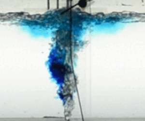
  $D_{m,b}$). A time sequence is shown in figure 2(a). The bubble curtain is violently bent first towards the light-fluid side (left) and then towards the dense-fluid side (right) in a ‘hook-like’ shape. Dense fluid (dyed in blue) penetrates through the bubble curtain into the light-fluid half, and reciprocally. The overall flow in the light-fluid half at a distance from the curtain resembles a lock-exchange flow. The bubble curtain mixes light and dense fluid around it. Due to the general up-flowing direction of the bubble curtain and the direction of the stack pressure forces, the mixed fluid appears to be mostly driven into the dense-fluid half. Apart from the presence of this mixed fluid, the flow in the dense-fluid half also looks similar to an intruding gravity current. In this breakthrough regime, the air flux is not strong enough for the bubble curtain to prevent the gravity current. This regime is defined by the competition between the vertical momentum of the bubble curtain (a rising plume of air and water) and the horizontal force exerted by the fluid around the curtain due to the initial horizontal stratification. When the momentum is too low, the curtain is overcome by the transverse force and is unable to separate the two halves of the tank. If the momentum is larger, the air curtain becomes more stable and the direct exchange across it becomes smaller.

Figure 2. Qualitative observations of different operating regimes of a bubble curtain. (a) Time sequence of the flow in the breakthrough regime for the air flux  $Q^{air}=20\,{\rm l}\,{\rm min}^{-1}$, the water depth $H=15\,{\rm cm}$ and the density difference $\Delta \rho =163\,{\rm kg}\,{\rm m}^{-3}$. (b) Time sequence of the flow in the curtain-driven regime for the air flux $Q^{air}=20\,{\rm l}\,{\rm min}^{-1}$, the water depth $H=15\,{\rm cm}$ and the density difference $\Delta \rho =30\,{\rm kg}\,{\rm m}^{-3}$. (c) Late frame of the time sequence shown in figure 2(b) ( $t=15.5\,{\rm s}$). The recirculation cell and the gravity current of mixed fluid originating from the cell are clearly visible in the left-hand half of the channel.
We note a distinct difference between the breakthrough regime for a bubble curtain and the breakthrough regime that is observed for single-phase air curtains, i.e. a real-scale air curtain in a building or a curtain consisting of a freshwater line jet in small-scale experiments. In the case of a single-phase air curtain, the upwards discharged curtain would be deflected entirely to the light-fluid side so that the gravity current in the upper half of the tank would be undisturbed. This difference arises due to the inherent slip velocity  $u_s$ of air bubbles. Due to this slip velocity $u_s$ the bubbles can escape the lateral deflection caused by the dense gravity current in the bottom half of the tank and cross the upper half of the tank where the light fluid forms an intruding gravity current into the dense fluid.
4.1.2. Curtain-driven regime
Once the vertical momentum flux of the bubble curtain is large enough to withstand the lateral stack pressure forces, the bubble curtain enters the so-called curtain-driven regime. A time sequence of this regime is shown in figures 2(b) and 2(c). At the very beginning of an experiment, the bubble curtain mixes surrounding fluid and drives it upwards. Upon reaching the free surface, the mixed fluid is deflected horizontally and all the bubbles escape out of the water due to the slip velocity  $u_s$ almost immediately. In particular, the escaping bubbles will change the buoyancy of the mixed fluid. The mixed fluid possesses a density which is larger than $\rho _l$ but less than $\rho _d$, so it behaves differently in the two halves of the tank. In the light-fluid half, the laterally deflected mixed fluid forms a recirculation cell of a finite horizontal extent. At some distance away from the curtain, there is a gravity current outflowing out of the recirculation cell along the bottom of the tank (see figure 2c). In the dense-fluid side, the quasi recirculation cell is less pronounced and the mixed fluid mostly outflows directly as a gravity current, though some mixing occurs and part of this mixed fluid is driven again back into the bubble curtain. The bubble curtain here acts as a separator between two sides of the channel and the exchange process is now due to the mixing induced by the bubble curtain itself.
4.2. Quantitative results
In our experiments, we observed that the slip velocity  $u_s$ of the bubbles was large enough such that all the bubbles escaped out of the water almost immediately after the bubble curtain impinged on the surface. Thus, the slip velocity $u_s$ is not included in the analysis of the infiltration flux $q_c$ or the recirculation cell that both arise due to the horizontally deflected fluid currents. We refer to § 6 for a discussion of the effects of a smaller slip velocity $u_s$.
4.2.1. Infiltration flux
After discussing the flow regimes that can occur for a bubble curtain, we present quantitative measurements of the infiltration flux  $q_c$ of dense fluid across the bubble curtain into the light-fluid half of the channel for a varying horizontal density difference $\Delta \rho$, water depth $H$ and the volume air flow rate $Q^{air}$ of the bubble curtain.
The infiltration flux per unit length  $q_c$ of dense fluid across the bubble curtain is calculated using the following procedure. We denote by $V$ the volume of fluid in the light-fluid side of the channel (so, the total water volume contained in the tank is $2V$) and by $V^{*}$ the volume of dense fluid intruding into the light-fluid side during an experimental run. The final water densities $\rho _l^{end}$ and $\rho _d^{end}$ in the channel at the end of an experiment obey the mass conservation
 \begin{equation} V\rho_l^{end} = (V-V^{*})\rho_l+V^{*}\rho_d, \end{equation}
where we implicitly assume that the net volume flux across the bubble curtain is zero.
The volume of dense fluid infiltrating the light-fluid side of the channel during an experiment is therefore
 \begin{equation} V^{*} = V \frac{\rho_l^{end}-\rho_l}{\rho_d-\rho_l}. \end{equation}
Hence, if  $t$ denotes the duration of an experiment, the infiltration flux of dense fluid per unit length is
 \begin{equation} q_c = \frac{V^{*}}{Wt}, \end{equation}
where  $W$ is the channel width.
We note that this way of calculating  $q_c$ does not account for the initial transients after the gate removal and the finite size effects of the tank. The flux $q_c$ in (4.3) is assumed to be steady, and for this to be valid the duration of the experiment should be chosen long enough for the transient effects to be negligible and short enough to avoid the effects of the finite channel length. We stopped our experimental runs at the time $t$ which was the moment shortly before the infiltrating gravity current reached the end wall of the channel. We will see later in § 5.4 whether such a choice of time $t$ was appropriate for all our experimental runs to guarantee the initial transient and finite geometry effects to be minimal.
Figure 3 shows the measured infiltration flux  $q_c$ (4.3) per unit length of dense fluid across the bubble curtain for our experiments. All the three panels in figure 3 possess the same legend which is displayed at the bottom.

Figure 3. Experimentally measured infiltration flux  $q_c$ per unit length of dense fluid across the bubble curtain.
Figure 3(a) plots  $q_c$ as a function of the relative horizontal density difference $\Delta \rho /\bar \rho$. We note that for the fixed water depth $H$ in the channel and the bubble curtain air flux $Q^{air}$, the infiltration flux $q_c$ is nearly constant for small values of $\Delta \rho /\bar \rho$ but rises sharply above a certain value of $\Delta \rho /\bar \rho$. The region of nearly constant $q_c$ corresponds to the curtain-driven regime in which the infiltration flux is due to the mixing by the bubble curtain whereas a sharp increase in $q_c$ indicates the breakthrough situation. The transition value of $\Delta \rho /\bar \rho$ between these two regimes depends on $Q^{air}$ and $H$. Furthermore, we observe that in the curtain-driven regime, the values of the infiltration flux $q_c$ noticeably increases with the water depth $H$ (symbols for a fixed colour). We can also detect a slight increase with the air flux $Q^{air}$ (colours for a fixed symbol) although it is less pronounced than the rise with $H$.
$H$.
The non-dimensionalised infiltration flux  $q_c(gq_{air})^{-1/3}/H$ is plotted as a function of $\Delta \rho /\bar \rho$ in figure 3(b). The scaling given by (2.18) yields a reasonable, albeit not a perfect, collapse of the data in the curtain-driven regime. The derivation of (2.18) was based on a simple physical picture of the bubble curtain entraining and spilling fluid to both sides of the channel. However, as explained in § 4.1.2, the real flow is more complicated with a pronounced recirculation cell building up next to the bubble curtain in the light-fluid half of the channel and the infiltrating gravity current of dense fluid propagating along the channel bottom and not next to the water surface. The non-negligible size of the recirculation cell compared with our finite channel length causes the variation of the scaled $q_c(gq_{air})^{-1/3}/H$ in the curtain-driven regime. We expect (2.18) to apply in the limit of an infinitely long channel. In § 5.2, we will develop a quantitative theoretical model for the calculation of $q_c$ which also will take into account the effects of the recirculation cell, and hence, the finite channel dimensions.
Finally, figure 3(c) illustrates the non-dimensionalised infiltration flux  $q_c(gq_{air})^{-1/3}/H$ as a function of the deflection modulus $D_{m,b}$ given in (2.5). We note a sharp transition between the breakthrough regime and a curtain-driven regime at approximately $D_{m,b}\approx 0.12$, or, equivalently, $Fr_{air}\approx 0.93$. This confirms that $D_{m,b}$ as defined in (2.5) is the governing parameter for the operating regime of the bubble curtain, similar to $D_m$ for air curtains. The transition value of $D_{m,b}\approx 0.12$ corresponds to the theoretically predicted transition value $D_m\approx 0.125$ for air curtains by Hayes & Stoecker (Reference Hayes and Stoecker1969b,Reference Hayes and Stoeckera). Furthermore, similar to air curtains (see (2.11), (2.12) and (2.16)), the infiltration flux $q_c$ appears to vary little with $D_{m,b}$ in the curtain-driven regime.
We note that the functional relationship between the non-dimensionalised infiltration flux  $q_c(gq_{air})^{-1/3}/H$ and the deflection modulus $D_{m,b}$ shown in figure 3(c) can also be established using a formal dimensional analysis.
The infiltration flux  $q_c$ across the bubble curtain can be written as a function of the variables in the problem as
 \begin{equation} q_c = f(g', H, B, L), \end{equation}
where we assume that the Boussinesq approximation applies. The length  $L$ is the horizontal distance that the intruding dense fluid propagates before the separation gate is closed. As explained in § 3, in our experiments $L$ corresponds just to the entire length of the light-fluid half. We can choose $H$ and $B$ as the repeating variables and form four dimensionless groups according to the Buckingham ${\rm \pi}$-theorem. These are
 \begin{equation} \frac{q_c}{B^{1/3}H}=\frac{q_c}{(gq_{air})^{1/3}H},\quad\frac{g' H}{B^{2/3}}\sim\frac{1}{D_{m,b}},\quad \frac{L}{H}. \end{equation}
Thus, in general, we expect a functional relationship
 \begin{equation} \frac{q_c}{(gq_{air})^{1/3}H} = f\left(D_{m,b},\frac{H}{L}\right). \end{equation}
Figure 3(c) shows  $q_c(gq_{air})^{-1/3}/H$ as a function of $D_{m,b}$ and neglects the dependence on $H/L$, which arises due to the finite channel dimensions. In § 5.2, we will derive a full functional relationship of the form (4.6).
4.2.2. Effectiveness of the bubble curtain
The purpose of using a bubble curtain in ship locks is to reduce salt intrusions into freshwater areas. In order to characterise the performance of a bubble curtain and in line with the effectiveness definition (2.19) for air curtains, we calculate the effectiveness for bubble curtains as
 \begin{equation} E = 1 - \frac{q_c}{q_{open}}. \end{equation}
We use (2.20) to calculate  $q_{open}$. Note that on dimensional grounds, $q_{open}$ for our channel is expected to scale as $q_{open}\sim H\sqrt {g'H}$. We keep the notation of the proportionality factor as $C_d/3$ and measure the discharge coefficient in a separate set of experiments presented in Appendix B. For our experimental set-up, $C_d\approx 0.55$.
Figure 4 plots the effectiveness  $E$ (4.7) as a function of $D_{m,b}$ (2.5). For low values of $D_{m,b}$ in the breakthrough regime, the effectiveness $E$ rises steeply. We observe that the maximum effectiveness of approximately $E\approx 0.8$ is achieved at the transition point $D_{m,b}\approx 0.12$, or $Fr_{air}\approx 0.93$, between the breakthrough and the curtain-driven regimes. For higher values of $D_{m,b}$ the effectiveness $E$ decreases, similar to how the effectiveness for air curtains also reduces with increasing $D_m$. We also observe an increased scatter in the data in the curtain-driven regime, creating an impression that $D_{m,b}$ might not be the correct parameter to collapse the data. However, as we will see in § 5.4, this is an artefact of the finite dimensions of our channel and the data are expected to collapse onto a single curve for an infinitely long channel.

Figure 4. Effectiveness  $E$ of the bubble curtain as a function of the deflection modulus $D_{m,b}$ for varying $\Delta \rho$, $H$ and $Q^{air}$.
We recall that for the time period when the initial transients and the finite size dimensions are negligible,  $E=1-{\textit {STF}}$. Based on their numerical simulations, Oldeman et al. (Reference Oldeman, Kamath, Masterov, O'Mahoney, van Heijst, Kuipers and Buist2020) reported a minimum value ${\textit {STF}}\approx 0.3$ for $Fr_{air}\approx 0.91$. This is in line with our measured maximum effectiveness value at $Fr_{air}\approx 0.93$, although our maximum effectiveness corresponds to ${\textit {STF}}\approx 0.2$. Oldeman et al. (Reference Oldeman, Kamath, Masterov, O'Mahoney, van Heijst, Kuipers and Buist2020) report two more data points of ${\textit {STF}}$ up to $Fr_{air}\approx 1.15$ that have slightly higher values than $0.3$. Our data presented in figure 4 comprise the data up until $Fr_{air}\approx 2.67$ and demonstrate a clear decrease in the effectiveness $E$, which corresponds to an increase in ${\textit {STF}}$. In particular, this clearly shows that the optimum operating regime of a bubble curtain is at $D_{m,b}\approx 0.12$, or equivalently at $Fr_{air}\approx 0.93$, which is the first explicit experimental confirmation for the optimum operating parameters of a bubble curtain.
4.2.3. Mixing cells in the curtain-driven regime
We examined the horizontal extent of the recirculation cells that appear in the curtain-driven regime (see § 4.1.2) in the light-fluid half of the channel. The measurements were conducted using the recorded images of experiments A. For each experimental run, 10 frames were chosen randomly during the steady phase of the flow, i.e. between the moment when the recirculation cell and the gravity current originating from it were clearly visible and the end of the experiment. These frames were then averaged and filtered. At each vertical height above the midheight of the channel, the horizontal extent of a cell was defined as the distance between the centre of the curtain and the point where the light intensity was the average between the average light intensity in the cell and that in the ambient fluid. The horizontal extent  $L_{cell}$ of the recirculation cell was then defined to be the average of these values. The results for the measured horizontal extent $L_{cell}$ as a function of the relative horizontal density difference $\Delta \rho /\bar \rho$ are shown in figure 5. The estimated error bars for the individual data points are within $2\text {--}3\,{\rm cm}$. The described procedure to determine the horizontal extent of the recirculation cells produced results that were consistent with their visually perceived boundaries.

Figure 5. The horizontal extent  $L_{cell}$ in metres of the recirculation cell in the curtain-driven regime plotted as a function of the relative horizontal density difference $\Delta \rho /\bar {\rho }$.
The most obvious trend is that the size  $L_{cell}$ of the cells decreases as the relative density difference $\Delta \rho /\bar {\rho }$ increases. Within the range of parameters involved in the experiments, the size of the cells is observed to vary by a factor of six. Varying the density difference alone within the given range, we can change the size of the cells by a factor of three. It can be seen in figure 5 that $L_{cell}$ increases with $Q^{air}$ but the influence of $H$ is less clear than that of the other two parameters. This is most likely because the water depth in our experiments ranges between $9\,{\rm cm}$ and $20\,{\rm cm}$, which is not sufficient to clearly delineate the effects of $H$. It can be expected that $L$ also scales with $H$ and $Q^{air}$ since these two parameters determine the effect of the curtain on the flow around it. Formally, we can write this using the dimensional analysis
 \begin{equation} L_{cell}=f(g',B,H), \end{equation}
where we again use the Boussinesq approximation and recall that  $B=gq_{air}$. We can now choose $g'$ and $H$ as our repeating variables, and invoking the Buckingham ${\rm \pi}$-theorem, we expect
 \begin{equation} \frac{L_{cell}}{H}=f\left(\frac{B}{(g'H)^{3/2}}\right). \end{equation}
In the next section, we provide some theoretical insights that explain our experimental measurements.
5. Theoretical modelling of experiments
The experiments revealed the existence of two operating regimes of the bubble curtain depending on the value of  $D_{m,b}$ that fundamentally differ in the mechanism of fluid exchange across the curtain: a nearly undisturbed lock-exchange flow in the breakthrough regime and an infiltration flow driven by the mixing induced by the curtain in the curtain-driven regime. The maximum effectiveness $E$ of the bubble curtain is achieved at the transition value of $D_{m,b}$ between these two regimes and starts to decrease slowly as $D_{m,b}$ is increased further in the curtain-driven regime. Since a bubble curtain acts as an effective separator between two sides of the channel at different densities only in the curtain-driven regime, we focus here on that regime and establish some theoretical models to explain and predict the observed flow behaviour. These theoretical considerations can be used to design a bubble curtain device that fits specific requirements and to understand the intrusions of salt in ship locks.
We note here that in the following theoretical considerations, we proceed with the assumption that the bubble size does not change as the bubble rises and the slip velocity  $u_s$ of the bubbles is high enough that the bubbles immediately escape out of the water upon reaching the surface. In other words, the buoyancy force due to the bubbles is constant with height and immediately disappears as the plume fluid flow is laterally deflected. Thus, the slip velocity $u_s$ of the bubbles is not taken into account in the derivation of the theoretical models in this section. We will discuss in § 6 how the bubble slip velocity $u_s$ could be included in a future expansion of the proposed models.
5.1. Scaling law for the cell size
We recall the scaling law for the line plume velocity
 \begin{equation} u\sim B^{1/3}\sim (g q_{air})^{1/3}, \end{equation}
that was discussed when we defined the deflection modulus  $D_{m,b}$ (2.5). We assume that the velocity of the horizontally deflected fluid after reaching the free surface will obey the same scaling (which was verified experimentally by Bulson (Reference Bulson1961)). The rising bubble plume mixes water from both sides, so the density difference between the horizontal flow next to the surface and the light-fluid side of the tank should be ${\sim}\Delta \rho$. Thus, the horizontally deflected fluid is subjected to the reduced gravity ${\sim}g'$ due to which it falls towards the bottom of the tank. The time for this process can be estimated as
 \begin{equation} t_{cell} \sim \sqrt{\frac{2H}{g'}}. \end{equation}
 Combining (5.1) and (5.2), we obtain a scaling prediction for the horizontal extent  $L_{cell}$ of the recirculation cell in the light-fluid half
 \begin{equation} L_{cell}\sim (g q_{air})^{1/3} \sqrt{\frac{2H}{g'}}. \end{equation}
 The experimentally measured values for the horizontal extent  $L_{cell}$ of the recirculation cell are plotted against the scaling (5.3) in figure 6. We observe a very satisfactory data collapse for $L_{cell}\lessapprox 0.5\,{\rm m}$, which is half the length of the light-fluid side. For higher values of $L_{cell}$, we expect the finite length of the channel to start affecting the flow. Furthermore, higher values of $(g q_{air})^{1/3} \sqrt {{2H}/{g'}}$ are mainly achieved by reducing $\Delta \rho$ in our experiments which renders an accurate measurement of $L_{cell}$ difficult since for small $\Delta \rho$ its boundaries may be blurred due to secondary flows and turbulent effects.

For  $L_{cell}\lessapprox 0.5\,{\rm m}$, we perform a linear fit of the data and obtain
 \begin{equation} L_{cell} \approx(0.62\pm 0.02)(g q_{air})^{1/3} \sqrt{\frac{2H}{g'}}. \end{equation}
We note here that the error in (5.4) is based on the 95 % confidence interval for the coefficient estimate of the linear regression model whereas an individual data point for the extent of the recirculation cell is determined within the accuracy of  $2\text {--}3\,{\rm cm}$ (see error bars in figure 6).
This can be rewritten as
 \begin{equation} \frac{ L_{cell}}{H} \approx(0.62\pm 0.02)\sqrt{2}\left(\frac{B}{(g'H)^{3/2}}\right)^{1/3}, \end{equation}
which is the functional relationship predicted by (4.9).
The recirculation cells around bubble curtains were studied by Fanneløp, Hirschberg & Küffer (Reference Fanneløp, Hirschberg and Küffer1991) and Riess & Fanneløp (Reference Riess and Fanneløp1998). Their experiments, however, were conducted in a homogeneous environment and did not include any density variations. McGinnis et al. (Reference McGinnis, Lorke, Wøest, Stöckli and Little2004) observed circulation patterns around bubble curtains in their field experiments in lakes that were vertically stratified. Keetels et al. (Reference Keetels, Uittenbogaard, Cornelisse, Villars and van Pagee2011) noted the presence of recirculation cells in their small-scale experiments on bubble curtains separating two sides at different densities but did not study the variation of the horizontal extent of the recirculation cells and how it depends on other parameters of the system.
The proportionality coefficient in (5.4) provides a good fit to our measured extents of recirculation cells in small-scale experiments. However, as will be discussed in § 6, it might be affected by the water depth  $H$ or the slip velocity $u_s$ and thus, might need to be adjusted for real-scale bubble curtains.
5.2. Model for the exchange through the curtain
Qualitative descriptions of the curtain-driven regime provided in § 4.1.2 indicate very clear features of the flow. A schematic of the flow is shown in figure 7.

Figure 7. Schematic of the steady flow in the curtain-driven regime. The right-hand side is initially filled with denser fluid and the left-hand side with lighter fluid. The notations used in the theoretical model are provided.
As before,  $\rho _l$ and $\rho _d$ are the initial densities of the light and dense fluids, respectively. We denote by $\rho _d'$ and $\rho _l'$ the densities of the weak quasi recirculation cell on the dense-fluid side and the recirculation cell on the light-fluid side, respectively, as is indicated in figure 7, and by $Q_H$ the volume flow rate of mixed fluid that the curtain discharges horizontally to each side upon reaching the water surface. The volume flow rate per unit width of the tank $W$ is denoted as $q_H$. To account for the recirculation, we denote the volume flow rate per unit width that leaves the cell on the light-fluid side as a gravity current as $\alpha q_H$ (or volumetric flow $\alpha Q_H$), on the dense-fluid side, as $\beta q_H$ (or $\beta Q_H$), where $\alpha <1$, $\beta <1$.
We have implicitly assumed that symmetry implies that the same volume flow of liquid per unit width  $q_H$ is discharged to each side. Similarly, we assume that the bubble curtain entrains the fluid equally from both sides, which is again $q_H$ in a steady state. We further postulate that the fluid in both recirculation cells (especially also in the quasi recirculation cell on the dense-fluid side) is well-mixed and that the gravity currents originating from them possess the same density: $\rho _d'$ or $\rho _l'$. We refer to figure 7 for a schematic of the involved flows.
The mass balance yields the density of the fluid rising within the plume as
 \begin{equation} \frac{1}{2}(\rho_l'+\rho_d'). \end{equation}
We can establish the mass balance equations in the recirculation cell in the light-fluid half as
 \begin{equation} \alpha q_H \rho_l + q_H \frac{1}{2}(\rho_l'+\rho_d') - \alpha q_H \rho_l' - q_H \rho_l' = 0 \end{equation}
and in the dense-fluid half as
 \begin{equation} \beta q_H \rho_d + q_H \frac{1}{2}(\rho_l'+\rho_d') - \beta q_H \rho_d' - q_H \rho_d' = 0. \end{equation}
This is equivalent to
 \begin{equation} \left(\begin{array}{cc}
-\tfrac{1}{2}-\alpha & \tfrac{1}{2}\\ \tfrac{1}{2} &
-\tfrac{1}{2}-\beta \end{array}\right)
\left(\begin{array}{c} \rho_l' \\ \rho_d'
\end{array}\right) = \left(\begin{array}{c} -\alpha\rho_l
\\ -\beta\rho_d \end{array}\right).
\end{equation}
\begin{equation} \left(\begin{array}{cc}
-\tfrac{1}{2}-\alpha & \tfrac{1}{2}\\ \tfrac{1}{2} &
-\tfrac{1}{2}-\beta \end{array}\right)
\left(\begin{array}{c} \rho_l' \\ \rho_d'
\end{array}\right) = \left(\begin{array}{c} -\alpha\rho_l
\\ -\beta\rho_d \end{array}\right).
\end{equation}
Therefore,
 \begin{equation} \left. \begin{aligned} \rho_l' & = \dfrac{\left(\tfrac{1}{2}+\beta\right)\alpha\rho_l+\tfrac{1}{2}\beta\rho_d}{\Delta} ,\\ \rho_d' & = \dfrac{\left(\tfrac{1}{2}+\alpha\right)\beta\rho_d+\tfrac{1}{2}\alpha\rho_l}{\Delta} , \end{aligned} \right\} \end{equation}
with
 \begin{equation} \Delta = \left(\frac{1}{2}+\alpha\right)\left(\frac{1}{2}+\beta\right)-\frac{1}{4} =\frac{\alpha+\beta}{2}+\alpha\beta. \end{equation}
Then, the equations for the gravity currents fluxes in both halves give (see (2.20))
 \begin{equation} \left. \begin{aligned} \alpha q_H & = \frac{C_d}{3}H^{3/2}g^{1/2}\left(\frac{\rho_l'-\rho_l}{\bar{\rho}}\right)^{1/2},\\ \beta q_H & = \frac{C_d}{3}H^{3/2}g^{1/2}\left(\frac{\rho_d-\rho_d'}{\bar{\rho}}\right)^{1/2}. \end{aligned} \right\} \end{equation}
 Solving the system (5.10) and (5.12) of four equations and four unknowns  $\rho _l'$, $\rho _d'$, $\alpha$ and $\beta$ yields
 \begin{gather} \alpha^{3}+\alpha^{2} = \frac{C_d^{2}}{18}\frac{H^{3} g'}{q_H^{2}}, \end{gather}
 \begin{gather}\alpha =\beta, \end{gather}
 \begin{gather}\rho_l'= \frac{\left(\frac{1}{2}+\alpha\right)\rho_l+\frac{1}{2}\rho_d}{\alpha + 1}, \end{gather}
 \begin{gather}\rho_d'= \frac{\left(\frac{1}{2}+\alpha\right)\rho_d+\frac{1}{2}\rho_l}{\alpha + 1}. \end{gather}
 The only obstacle with respect to the comparison of this model with our experiments is the unknown value of the volume flux per unit length  $q_H$. The dimensional scaling inspired by Morton et al. (Reference Morton, Taylor and Turner1956) that has been previously discussed is
 \begin{equation} q_H \sim (g q_{air})^{1/3} H. \end{equation}
 It is important, however, to determine the order of magnitude of the coefficient that goes with the scaling since the model we have developed is not a scaling law but aims at predicting the values as precisely as possible. Abraham et al. (Reference Abraham, van der Burgh and DeVos1973) suggest that the depth of the outflowing current is  $H/4$ and that the velocity increases linearly from a zero value at the lower boundary of the current to a maximum value at the water surface. Bulson (Reference Bulson1961) measured that the maximum surface velocity $V_{max}$ of the horizontal current created by a line bubble plume scales as
 \begin{equation} V_{max} \approx C_v (g q_{air})^{1/3} \end{equation}
with the proportionality factor  $C_v\approx 1.46$.
This results in
 \begin{equation} q_H \approx \frac{1}{2}V_{max}\frac{H}{4}=\frac{C_v}{8}(g q_{air})^{1/3} H\approx 0.18 (g q_{air})^{1/3} H. \end{equation}
We conducted some experiments to examine whether the scaling (5.18) is appropriate in our case (at our small scale, in particular) that are briefly presented in Appendix C.
5.3. Comparison between model and experiments
We now use the model developed in the previous section in order to predict the infiltration flux  $q_c^{th}$ of dense fluid across the bubble curtain during an experimental run and compare it with the experimentally measured flux $q_c$ (4.3). Note that the superscript ‘th’ stands for ‘theoretical’.
The procedure to calculate  $q_c^{th}$ is as follows. First, we use (5.13) to determine the value of the parameter $\alpha$ for each experimental run. The right-hand side of (5.13),
 \begin{equation} \frac{C_d^{2}}{18}\frac{H^{3}g'}{q_H^{2}}=\frac{64C_d^{2}}{18C_v^{2}}\frac{Hg'}{(gq_{air})^{2/3}}=\frac{64C_d^{2}\alpha_E}{9C_v^{2}}\frac{1}{D_{m,b}}\approx\frac{0.072}{D_{m,b}}, \end{equation}
where we use (5.19) for  $q_H$, contains the known initial condition $D_{m,b}$ along with proportionality coefficients measured in the previous literature and can be calculated directly for every experimental run. Equation (5.13) is then solved for $\alpha$. This yields one well-defined positive root $0<\alpha <1$ for any choice of initial conditions for which the bubble curtain is operating in the curtain-driven regime. A short proof of this statement is provided in Appendix D.
Once the value of  $\alpha$ is found, the infiltration flux $q_c^{th}$ is calculated as
 \begin{equation} q_c^{th}=\left(\alpha q_H+\frac{L_{cell}H}{2t}\right)\frac{1}{2(\alpha+1)}, \end{equation}
where  $L_{cell}$ can be computed using the correlation (5.4). Figure 8 elucidates the two terms inside the brackets contributing to the infiltration flux. The first term, $\alpha q_H$, is due to the gravity current propagating along the channel bottom. The second term, $L_{cell}H/2t$, arises because of the presence of the recirculation cell in the upper half of the channel next to the bubble curtain. It is calculated as the volume in the upper half of the recirculation cell $L_{cell}H/2$, which is fixed once the recirculation cell is established and is shown in the blue dashed square in figure 8, divided by the time $t$. We recall that we consider only those times $t$ which are longer than the initial transient time during which the recirculation cell is establishing. Note that this correction due to the recirculation cell decreases with an increasing duration $t$ of an experiment. The fluid inside the dyed volume in the light fluid possesses the density
 \begin{equation} \rho_l'=\frac{(1+2\alpha)\rho_l+\rho_d}{2(\alpha+1)}. \end{equation}
This means that a fraction of  $(1+2\alpha )/(2(\alpha +1))$ of fluid inside the dyed volume originates from the light-fluid half whereas a fraction of $1/(2(\alpha +1))$ is the original dense fluid that has infiltrated the light-fluid half across the bubble curtain. This explains the presence of the factor $1/(2(\alpha +1))$ in the calculation of the theoretical infiltration flux (5.21).

Figure 8. Sketch of the light-fluid half of the channel illustrating two volume contributions of the dyed fluid in the calculation of the theoretical infiltration flux  $q_c^{th}$ in (5.21).
Figure 9 shows the comparison between the experimentally measured flux  $q_c$ across the bubble curtain in experiments A and the theoretically expected infiltration flux $q_c^{th}$ calculated using (5.21) with (5.19) and (5.4). We observe a near perfect collapse of the data around the line $q_c=q_c^{th}$ which shows that our theoretical model makes an excellent prediction of the infiltration flux. We can calculate the mean deviation of the experimentally measured values from the bisectrix of the first quadrant as $\sqrt {{\sum }_i(q_c(i)-q_c^{th}(i))^{2}/N}\approx 2.1\,\textrm {cm}^{2}\,\textrm {s}^{-1}$, where the index $i$ runs through our experiments and $N$ is the total number of our measurements. We note here, however, that our model does not take into account any reflections of the intruding gravity current from the end wall of the tank.

Figure 9. Experimentally measured values of the infiltration flux per unit length  $q_c$ of dense fluid across the bubble curtain plotted against the theoretically expected infiltration flux per unit length $q_c^{th}$. We use (5.21) with (5.19) and (5.4) to calculate $q_c^{th}$ where $\alpha$ is determined for every set of initial conditions by (5.29). The black line depicts $q_c=q_c^{th}$.
We note that (5.21) presents the functional relationship given by (4.6). The time  $t$ can be linked to the horizontal propagation distance $L$ of the intruding gravity current as
 \begin{equation} t = \frac{3 L}{2C_d\sqrt{\dfrac{g(\rho_l'-\rho_l)}{\bar\rho}H}}=\frac{3L\sqrt{2(\alpha+1)}}{2C_d\sqrt{g'H}}, \end{equation}
where we apply (5.12) and model the intruding volume as  $\alpha q_H t = LH/2$. Then, using (5.19) and (5.4) we obtain
 \begin{align} \frac{q_c^{th}}{(gq_{air})^{1/3}H}&=\left(C_1\alpha+C_2\frac{1}{\sqrt{2(\alpha+1)}}\times\sqrt{\frac{H}{g'}}\times\frac{\sqrt{g'H}}{L}\right)\frac{1}{2(\alpha+1)}\nonumber\\ &=\left(C_1\alpha+C_2\frac{1}{\sqrt{2(\alpha+1)}}\times\frac{H}{L}\right)\frac{1}{2(\alpha+1)}, \end{align}
where  $\alpha = \alpha (D_{m,b})$ and $C_1$ and $C_2$ are constant coefficients. This is exactly the form of the functional relationship (4.6) expected from the dimensional analysis.
For an infinitely long horizontal propagation distance  $L$ (or, equivalently, for $t\to \infty$)
 \begin{equation} \frac{q_c^{th}}{(gq_{air})^{1/3}H}\to C_1\frac{\alpha}{2(\alpha+1)}, \end{equation}
which is equivalent to
 \begin{equation} q_c^{th}\to \frac{\alpha}{2(\alpha+1)}q_H. \end{equation}
We see that in this case, the non-dimensionalised infiltration flux is a function only of the deflection modulus, so that the scatter observed in figure 3(c) is an artefact of the finite length of our tank. We also recover the scaling proposed in (2.18) with the proportionality factor depending on  $D_{m,b}$ as argued in (5.20). Thus, in contrast to the relation given by (2.16) for air curtains, the ratio $q_c/q_H$ for a bubble curtain is not constant with $D_{m,b}$ for a fixed opening geometry in the curtain-driven regime. However, as figure 3(c) indicates, the variation of $q_c/q_H$ with $D_{m,b}$ in the curtain-driven regime is relatively slow.
Figure 8 allows us to estimate the relative contributions of the terms  $\alpha q_H$ and $L_{cell}H/2t$ to $q_c^{th}$ in (5.21). The first term dominates if the volume $\alpha q_H t$ is larger than the volume $L_{cell}H/2$, that is for those times $t$ when the recirculation cell is already established and the gravity current starts to flow out of the recirculation cell. Nevertheless, the correction due to the second term can be significant for a fixed finite length of the channel. Recall that we stopped our experiments when the gravity current reached the end wall of the light-fluid side. If, for example, the horizontal extent of the recirculation cell is half the length of the light-fluid side, then the correction due to the recirculation cell will be 50 %. We can assess the relative contribution of the correction due to the recirculation cell in our experiments by defining
 \begin{equation} q_c^{th,approx}=\frac{\alpha q_H}{2(\alpha+1)}, \end{equation}
which neglects the second term of (5.21). Figure 10 shows the experimentally measured flux  $q_c$ against the approximate infiltration flux $q_c^{th,approx}$ (calculated using (5.27) with (5.19)). The horizontal distance between the axis of ordinates and a point is the contribution due to the term $\alpha q_H$, the horizontal distance between a point and the bisectrix of the first quadrant (shown as a black line) is the missing contribution due to the term $L_{cell}H/2t$ in (5.21).

Figure 10. Experimentally measured values of the infiltration flux per unit length  $q_c$ of dense fluid across the bubble curtain plotted against the approximate infiltration flux per unit length $q_c^{th,approx}$ given by (5.27). The black line depicts the bisectrix of the first quadrant.
5.4. Effectiveness revisited
After establishing the model (5.13)–(5.16) allowing us to calculate the theoretical infiltration flux  $q_c^{th}$ in (5.21), we revisit the effectiveness measurements presented in § 4.2.2 and can now explain the observed scatter in the experimental data for large $D_{m,b}$.
For  $t\to \infty$, we can deduce that theoretically
 \begin{align} E&= 1-\frac{q_c^{th}}{q_{open}}\nonumber\\ &\to 1-\frac{\frac{\alpha}{2(\alpha+1)}\frac{C_v}{8}(gq_{air})^{1/3}H}{\frac{C_d}{3}H\sqrt{g'H}}\nonumber\\ &= 1-\frac{3\alpha C_v}{16C_d(\alpha+1)}\frac{\sqrt{D_{m,b}}}{\sqrt{2\alpha_E}}, \end{align}
where  $\alpha$ is given by
 \begin{equation} \alpha^{3}+\alpha^{2}=\frac{64C_d^{2}\alpha_E}{9C_v^{2}}\frac{1}{D_{m,b}}. \end{equation}
 This demonstrates that for  $t\to \infty$, the effectiveness $E$ can be expressed as a function of $D_{m,b}$ and we would expect the collapse of our measured data. The data scatter observed in figure 4 arises from the presence of the recirculation cell and the fact that our channel is not long enough to achieve the asymptotic scaling for the infiltration flux. Thus, it is an artefact of the finite dimensions of our channel. Indeed, if we superimpose the curve $E(D_{m,b})$ as given in (5.28) and (5.29) on our data as shown in figure 11, we observe that it constitutes the upper envelope of the measured data points. The data points for $H=9\,\textrm {cm}$ (diamonds) are closer to our theoretical limit than for $H=20\,\textrm {cm}$ (squares), which is the expected behaviour because of the smaller aspect ratio $H/L$ for $H=9\,\textrm {cm}$.

Figure 11. Theoretical curve  $E(D_m)$ in the limit $t\to \infty$ for an infinitely long channel calculated by means of (5.28) and (5.29). The experimentally measured effectiveness values (cf. figure 4) are below the theoretical curve due to the presence of the recirculation cell next to the bubble curtain and the finite length of the channel.
We stress here, in particular, that our theoretical model enables us to provide a theoretical upper limit on the effectiveness values of the bubble curtain by means of (5.28) and (5.29). The optimum effectiveness at  $D_{m.b}\approx 0.12$ can be theoretically calculated as $E\approx 0.83$. We also observe that for $D_{m.b}\to \infty$, we obtain $E\to 1-1/2\sqrt {2}\approx 0.65$.
5.5. Instantaneous density measurements in experiments B
Our set of model equations (5.13)–(5.16) allows not only the calculation of the infiltration flux  $q_c^{th}$ but also the prediction of the asymptotic values of densities $\rho _l'$ and $\rho _d'$.
Experiments B provide instantaneous and local density measurements in the curtain-driven regime by means of dye attenuation as explained in § 3.2. In particular, processing the data from an experiment B (see Appendix A) shows the temporal evolution of  $\rho _{l,exp}'(t)$ and $\rho _{d,exp}'(t)$ in the recirculation cells. This can confirm that a steady state has indeed been reached and allows for a comparison between the predicted final values of $\rho _l'$ and $\rho _d'$ given in (5.15) and (5.16) and their measured final counterparts $\rho _{l,exp}'$ and $\rho _{d,exp}'$.
The quantitative results for the final densities  $\rho _{l,exp}'$ and $\rho _{d,exp}'$ in experiments B are shown in table 1 while figure 12 shows a few examples of how $\rho _{l,exp}'(t)$ and $\rho _{d,exp}'(t)$ evolve over time. The examples provided in figure 12 show that the densities $\rho _{l,exp}'(t)$ and $\rho _{d,exp}'(t)$ in each half of the channel tend towards a constant value. The evolution $\rho _{l,exp}'(t)$ is steep near the beginning and quickly reaches its constant, asymptotic value. In contrast, the decrease of $\rho _{d,exp}'(t)$ is more stable and slower. An explanation for this asymmetry is that the flow itself is initially highly asymmetric around the bubble curtain. Indeed, on the dense-fluid side, the bubble curtain impinging on the surface immediately creates an outflowing gravity current which propagates in the upper half of the channel. Over time, some mixing occurs and some part of this mixed fluid is re-entrained by the bubble curtain giving rise to a weak quasi recirculation cell. In the light-fluid side, however, the fluid spilled laterally by the bubble curtain first sinks to the bottom and creates a recirculation cell so that this fluid can be re-entrained by the bubble curtain. Based on this physical picture, we indeed expect that the transient phase of $\rho _{d,exp}'(t)$ in the dense-fluid side will be longer because mixed fluid will require a longer time to recirculate.

Figure 12. Examples of the temporal evolution of densities  $\rho _{l,exp}'$ (red line) and $\rho _{d,exp}'$ (blue line) in experiments B. The dashed lines indicate their respective theoretical predictions $\rho _l'$ and $\rho _d'$. The time $t$ is real time with the $t=0\,\textrm {s}$ corresponding to the gate removal at the start of an experiment. Here (a) $Q^{air}=10\,\textrm {l}\,\textrm {min}^{-1}$, $H=9\,\textrm {cm}$, $\Delta \rho =12\,\textrm {kg}\,\textrm {m}^{-3}$; (b) $Q^{air}=30\,\textrm {l}\,\textrm {min}^{-1}$, $H=15\,\textrm {cm}$, $\Delta \rho =12\,\textrm {kg}\,\textrm {m}^{-3}$; (c) $Q^{air}=10\,\textrm {l}\,\textrm {min}^{-1}$, $H=9\,\textrm {cm}$, $\Delta \rho =25\,\textrm {kg}\,\textrm {m}^{-3}$; (d) $Q^{air}=30\,\textrm {l}\,\textrm {min}^{-1}$, $H=15\,\textrm {cm}$, $\Delta \rho =25\,\textrm {kg}\,\textrm {m}^{-3}$.
Table 1. Quantitative comparison of  $\rho _l'$ and $\rho _d'$ with their measured final counterparts $\rho _{l,exp}'$ and $\rho _{d,exp}'$ in experiments B. The measurement error in the density using the dye attenuation is approximately $1\,\textrm {kg}\,\textrm {m}^{-3}$.

Figure 13 shows the ratios  $(\rho _{l,exp}'-\rho _l')/\Delta \rho$ and $(\rho _{d,exp}'-\rho _d')/\Delta \rho$ of the 17 experiments listed in table 1. Given the measurement errors using the dye attenuation technique explained in § 3.2 and Appendix A, we observe that predicted values of $\rho _l'$ in (5.15) are very close to experimental measurements for $\rho _{l,exp}'$: the discrepancy is always within 10 % of the initial density difference $\Delta \rho$ and is in almost all experiments within $1\,\textrm {kg}\,\textrm {m}^{-3}$. There is, however, a bigger discrepancy when it comes to $\rho _d'$, with differences between the model and the experiments that sometimes reach $4\,\textrm {kg}\,\textrm {m}^{-3}$. In all experiments $\rho _{d,exp}'$ is underestimated by the theoretical values for $\rho _d'$ in (5.16). This may be a consequence of the fact that a steady state on the dense-fluid side is not quite reached in our experiments, as argued below.

Figure 13. The relative differences  $(\rho _{l,exp}'-\rho _l')/\Delta \rho$ (red diamonds) and $(\rho _{d,exp}'-\rho _d')/\Delta \rho$ (blue circles) of the 17 experiments listed in table 1.
As a side remark, we note that the asymptotic values of  $\rho _l'$ and $\rho _d'$ (or $\rho _{l,exp}'$ and $\rho _{d,exp}'$, respectively) are not the same: there is still a density difference between the recirculation cells on either side of the bubble curtain in the steady state. The difference between $(\rho _d-\rho _l)/2$ and both $\rho _l'$ and $\rho _d'$ gives an idea of how imperfectly the curtain acts as a mixing device. Indeed, if it were a perfectly efficient mixer we would have a fluid of perfectly homogeneous density around it. With our model $\rho _d'-\rho _l'=\alpha (\rho _d-\rho _l)/(\alpha +1)$, which goes to 0 as $D_{m,b}\to \infty$.
The results provided in table 1 and figure 12 are obtained by averaging the information collected in experiments B over the recirculation cells (see Appendix A). In order to try to understand the quasi-systematic discrepancy between the predicted values of  $\rho _d'$ and the measured values $\rho _{d,exp}'$, it is useful to consider the density maps inside the tank.
Figure 14 shows a density map for  $Q^{air}=30\,\textrm {l}\,\textrm {min}^{-1}$, $H=15\,\textrm {cm}$ and $\Delta \rho =25\,\textrm {kg}\,\textrm {m}^{-3}$. The quantitative data for this particular experiment B15 are listed in table 1 and the evolution of the density in both cells is shown in figure 12. At the end of the experiment, there is a noticeable volume of fluid at the bottom of the tank below the recirculation cell in the dense-fluid half (right-hand side of the tank), that is denser than the cell. This phenomenon was not taken into account in the theoretical model (see § 5.2) which could explain why there is a discrepancy between the model and the experiments in terms of $\rho _d'$.

Figure 14. Density map in  $\textrm {kg}\,\textrm {m}^{-3}$ obtained with data from experiment B15 for $Q=30\,\textrm {l}\,\textrm {min}^{-1}$, $H=15\,\textrm {cm}$ and $\Delta \rho =25\,\textrm {kg}\,\textrm {m}^{-3}$.
It is an interesting question where this bottom layer of fluid which is denser than the recirculation cell density  $\rho _d'$ comes from. It could either consist of the dense fluid $\rho _d$ that is attracted along the bottom of the channel by the entrainment flow created by the bubble curtain and, thus, would continue to exist in the final steady state. Alternatively, it could be the original boundary layer of pure dense fluid that slowly disappears as the quasi recirculation cell slowly builds up, but would in our case take more time to disappear than the experiment lasts. In this latter case, we expect $\rho _{d,exp}'(t)\to \rho _d'$ as $t\to \infty$, but the time for the final steady state in the dense-fluid side to be reached would be longer than the duration of our experiments.
A simple experiment was conducted to understand what happens at the bottom of the channel in the dense-fluid side. The set-up was the same as in experiment A (see § 3.1) except that the dense fluid was filled into the half of the channel where the water was still before the removal of the sealing gate, i.e. the left-hand side of the channel in the recorded videos. Some dyed dense fluid was carefully injected at the bottom of the dense-fluid half with the least possible momentum in order to create a stable bottom layer of dyed fluid in the dense-fluid half of the channel. This dyed layer at the bottom allows the visualisation of the flow at the bottom of the tank in the dense-fluid half. We qualitatively observed that the bottom dyed layer in the vicinity of the bubble curtain was slowly disappearing by mixing into the recirculation cell and its colour was gradually fading out. We did not observe any significant flow of dense dyed fluid along the channel bottom caused by the entrainment of the bubble curtain.
Based on this qualitative experiment, it appears that the layer of denser fluid underneath the recirculation cell observed in figure 14 is most likely the initial bottom layer of the dense fluid that is still in the process of being slowly mixed. In particular, based on our experimental observations we can estimate that the time it takes for the initial bottom layer of dense fluid to disappear and the steady state to be reached is longer than the duration of our dye attenuation experiments: in figure 15, we can observe that the dyed fluid from the bottom layer is still not entirely mixed after  $t=40\,\textrm {s}$ which is a typical duration of experiments B. Summarising, we expect that in the steady state $\rho _{d,exp}'(t)\to \rho _d'$. However, the times needed to reach this steady state are longer than the running times we were able to achieve in our dye attenuation measurements in experiments B. This is also corroborated by the observation of the blue curves in figure 12 that still appear to slowly decrease.

Figure 15. Time sequence of an experiment where only a thin layer of dense fluid is dyed at the bottom (the dense fluid is on the left and the light fluid is on the right) with  $Q=20\,\textrm {l}\,\textrm {min}^{-1}$, $H=15\,\textrm {cm}$ and $\Delta \rho =25\,\textrm {kg}\,\textrm {m}^{-3}$.
6. Discussion
In our small-scale experiments, the rising bubbles creating the bubble curtain had two distinctive features. First, the bubble size did not change as the bubbles were rising through the water column and, second, the slip velocity  $u_s$ of the bubbles was large enough that all the bubbles almost immediately escaped out of water as the curtain impinged on the surface rather than being laterally deflected by the horizontal outflowing currents. These were the two assumptions used in our theoretical modelling in § 5. Bubble plumes in real-scale water reservoirs with a depth of several metres exhibit variation in the buoyancy with height because of the bubble size expansion due to the hydrostatic pressure changes (Ditmars & Cederwall Reference Ditmars and Cederwall1974; Milgram Reference Milgram1983) as well as the gas exchange with the surrounding fluid (Wüest, Brooks & Imboden Reference Wüest, Brooks and Imboden1992; McGinnis & Little Reference McGinnis and Little2002; McGinnis et al. Reference McGinnis, Lorke, Wøest, Stöckli and Little2004). Furthermore, the slip velocity of the bubbles $u_s$ might be small enough that the bubbles are laterally deflected by horizontal currents when the curtain impinges on the water surface or in the breakthrough regime. Here, we discuss the applications and limitations of our model to real-scale bubble curtains.
Assuming the hydrostatic pressure distribution and the isothermal expansion of bubbles, the buoyancy flux varies with the vertical coordinate  $z$ as
 \begin{equation} B(z)=\frac{\dfrac{p_{atm}}{\bar\rho g}+H}{\dfrac{p_{atm}}{\bar\rho g}+(H-z)}gq_{air}, \end{equation}
where  $p_{atm}$ is the atmospheric pressure at the water surface.
For  $H=10\,\textrm {m}$, the buoyancy flux close to the surface would be $B(H)=2gq_{air}$ and for $H=5\,\textrm {m}$, $B(H)=3gq_{air}/2.$ However, as we see from (5.4), (5.19) and (5.21), the buoyancy flux enters the equations only with the power of $1/3$. So, for a channel of 5 m depth, the correction due to the changing buoyancy flux would be at most 15 %. As a side note, the uncertainty of 10 % in measuring $q_{air}$ at the low end of our parameter range in small-scale experiments, yields only a 3 % error for our measurements of $q_c$.
In fact, as can be seen in (6.1), the correction due to the changing buoyancy flux can be absorbed into the proportionality coefficients that would depend on the water depth  $H$ whereas the functional form of (5.4), (5.19) and (5.21) would remain the same. For example, in (5.19), this means defining $C_v(H)$ and measuring it for different water depths. However, the fact that to analyse our small-scale experiments we used the coefficient $C_v$ measured in real-scale experiments by Bulson (Reference Bulson1961) and obtained a good fit of the data with our model, suggests that this dependence should not be too pronounced (see also van der Ven & Wieleman Reference van der Ven and Wieleman2017).
Another mechanism by which the buoyancy flux can vary is the gas exchange via dissolution and stripping between the air bubbles and the dissolved oxygen and nitrogen in the surrounding water. This process is the main principle used for the hypolimnetic oxygenation of lakes and other water reservoirs (Wüest et al. Reference Wüest, Brooks and Imboden1992; McGinnis & Little Reference McGinnis and Little2002; McGinnis et al. Reference McGinnis, Lorke, Wøest, Stöckli and Little2004). However, the bubble plumes used for aeration are relatively weak such that the bubbles are all expected to dissolve in water. For bubble curtains, we can make the following estimate. For a stable bubble curtain, we need  $D_{m,b}\gtrapprox 0.12$, which yields
 \begin{equation} q_{air}=\frac{1}{g}\left(\frac{D_{m,b}Hg'}{2\alpha_E}\right)^{3/2}\gtrapprox 0.22\,{\rm m}^{2}\,{\rm s}^{{-}1}\approx 800\,{\rm m}^{2}\,{\rm h}^{{-}1}, \end{equation}
where we take as representative values  $g'=0.2\,\textrm {m}\,\textrm {s}^{-2}$ and $H=5\,\textrm {m}$. This value is $10^{3}$ times larger than the gas flow rate used for the oxygenation of lakes (McGinnis & Little Reference McGinnis and Little2002). The associated mass flux per unit width is approximately $270\,\textrm {g}\,\textrm {m}^{-1}\,\textrm {s}^{-1}$. Taking the solubility of gases (nitrogen and oxygen) in water to be approximately $0.04\,\textrm {g}\,\textrm {l}^{-1}=40\,\textrm {g}\,\textrm {m}^{-3}$, around $200\,\textrm {g}$ of gas can be dissolved in the water column of $1\,\textrm {m}^{2}$ cross-sectional area and $5\,\textrm {m}$ height around the bubble curtain. This means that after $1\,\textrm {s}$ the bubble curtain supplies more gas bubbles than can be dissolved in such a surrounding water column. Thus, we can conclude that the gas exchange does not noticeably change the buoyancy flux of the bubble curtain. We also note here that Bombardelli et al. (Reference Bombardelli, Buscaglia, Rehmann, Rincón and Garcıa2007) provided a full numerical solution of the model by Wüest et al. (Reference Wüest, Brooks and Imboden1992) including mass transfer and compressibility effects for a realistic water reservoir and showed that for the bubble sizes between 2 mm and 7 mm the assumption of a constant bubble radius is acceptable.
Additionally, in the derivation of our model for the infiltration flux, we neglected the inner structure of the bubble curtain, which is a multiphase line plume: the bubbles merely provided the buoyancy driving the plume, that immediately disappeared as the curtain reached the water surface. As a consequence, we did not measure the bubble size distribution in our small-scale experiments and our suggested models for the length of the recirculation cells (5.4) and the infiltration flux (5.21) do not include the slip velocity  $u_s$.
The effects of different slip velocities  $u_s$ are twofold. First, the entrainment constant $\alpha _E$ might depend on the slip velocity $u_s$ of the bubbles as well as on the gas flow rate (cf. Milgram Reference Milgram1983) which will change the volume flux in the rising bubble curtain. In our theoretical modelling, however, we have not explicitly used the volume flux in the bubble curtain but rather the flux $q_H$ (5.19) which we based on the experimental correlation obtained by Bulson (Reference Bulson1961) for real-scale bubble plumes. Thus, we expect the expression for $q_H$ to equally hold for real-scale bubble curtains. This also means that the expression for $\alpha$ (5.13) is expected to remain valid for the real-scale bubble curtains, and, hence the formulas for $\rho _l'$ and $\rho _d'$ given by (5.15) and (5.16), respectively.
Second, the slip velocity  $u_s$ determines how easily the bubbles are laterally deflected. In our experiments, the slip velocity $u_s$ was large enough for the bubbles to almost immediately escape out of water as the bubble curtain impinged on the surface. For real-scale bubble curtains, the bubble sizes in the millimetre range possess slip velocities $u_s=0.3\,\textrm {m}\,\textrm {s}^{-1}$ (Wüest et al. Reference Wüest, Brooks and Imboden1992). As the bubble curtain flow is laterally deflected upon reaching the surface, the bubbles must cross the maximum distance $\sim H/4$ to reach the surface and thus, we expect all the bubbles to escape at a time scale $\sim H/4u_s$. This time scale should be contrasted with the time scale $\sqrt {2H/g'}$ for the formation of the recirculation cells. For $H=5\,\textrm {m}$ and $g'=0.2\,\textrm {m}\,\textrm {s}^{-2}$, we can calculate the ratio of both time scales to be approximately 0.5. This means that the bubbles will remain suspended in the laterally deflected flows for a non-negligible amount of time and only gradually disappear. Hence, we can expect the buoyancy of the laterally deflected flows to gradually change over time and, as a consequence, the horizontal extent of the recirculation cells might be larger than predicted by (5.4), and the infiltration flux in (5.21) might increase due to the growing contribution of $L_{cell}$. We expect, however, the functional dependence of $L_{cell}$ on $g'$,
$g'$,  $q_{air}$ and $H$ to remain the same and the proportionality factor could be modelled as a function of $u_s$. It would be an interesting problem for a future study to investigate the dependence of the horizontal extent of recirculation cells on the slip velocity $u_s$. We also note here that in the breakthrough regime, the path of the rising bubbles in our small-scale experiments may be different from the path of the bubbles in the breakthrough regime for real-scale bubble curtains. However, since the bubble curtain does not act as an effective barrier in the breakthrough regime, this observation is of no further relevance to our study.
Summarising the preceding discussion, we might expect the form of the functional relationships for  $L_{cell}$, $q_H$, $q_c^{th}$, $\rho _l'$ and $\rho _d'$ to apply to real-scale air curtains although some of the proportionality coefficients may change depending on the water depth $H$ and the slip velocity of the bubbles $u_s$. Some further experiments on a larger scale would be desirable to understand the effects of $H$ and $u_s$ on these experimentally measured coefficients.
7. Conclusion
In this paper, we considered both experimentally and theoretically the ability of a bubble curtain to separate two water zones at different densities. Our small-scale experiments provide the most exhaustive investigation of the bubble curtain performance for varying density differences, air fluxes and water depths to date.
We first established a formal analogy between a bubble curtain and an air curtain and showed how the two theoretical frameworks used for their description can be unified. In particular, analogous to air curtains, we identified two operating regimes of the bubble curtain: the breakthrough regime, where the bubble curtain is too weak to stop the buoyancy-driven exchange flow, and the curtain-driven regime, where the bubble curtain successfully interrupts the gravity current. In the latter regime, the infiltration flux of dense fluid is solely due to the self-induced mixing of the bubble curtain. Both our theoretical reasoning and our quantitative measurements allowed us to conclude that the bubble curtain operates optimally at  $D_{m.b}\approx 0.12$, or $Fr_{air}\approx 0.93$, which is the value at the transition between the breakthrough and the curtain-driven regimes.
In the curtain-driven regime, we developed a theoretical model to predict the infiltration flux of dense fluid across the bubble curtain, the density inside the recirculation cells as well as the horizontal extent of the mixing cells in the light-fluid half. Our theoretical predictions for the infiltration flux across the bubble curtain are in excellent agreement with our measured data. This also allowed us to provide an upper limit on the effectiveness of the bubble curtain in the curtain-driven regime and show that, asymptotically for very long running times, the values for the effectiveness  $E$ are expected to collapse onto a single curve as a function of $D_{m.b}$. The optimum effectiveness achieved at $D_{m.b}\approx 0.12$ can be theoretically estimated to be $E\approx 0.83$. The prediction of the density $\rho _l'$ in the recirculation cell in the light-fluid half coincides very well with the measured values $\rho '_{l,exp}$. There is a slight discrepancy between the density $\rho _d'$ and the experimentally measured $\rho '_{d,exp}$ in the quasi recirculation cell in the dense-fluid side. However, we attribute this difference mostly to the fact that the running times of our experiments were not long enough to achieve a steady state in the dense-fluid side due to the limited size of our experimental set-up.
We may expect that our results and theoretical models derived from small-scale experiments apply to real-scale bubble curtains and can be helpful in minimising the salt transport from saltwater into the freshwater zone, which is the main goal of using a bubble curtain. For instance, the effectiveness reaches its peak at  $D_{m.b}\approx 0.12$. Thus, when operating a bubble curtain, the air flux $q_{air}$ could be adjusted for given $H$ and $g'$ to ensure the optimal performance of the bubble curtain. Our model developed in § 5.2 allows us to theoretically calculate the infiltration flux $q_c$ across the bubble curtain via (5.21). For example, it would allow an estimate of the maximum time that a lock can remain open if the objective is to keep the salt transport below a given acceptable level. The theoretical expression (5.21) for the infiltration flux could also be incorporated into models simulating the entire system of channels with multiple locks to estimate the salt intrusion into the system for a given ship traffic.
Summarising, the bubble curtain can be highly effective in preventing the saltwater intrusion with the effectiveness value  $E$ of 80 %. As we mentioned earlier, however, the definition of effectiveness does not take into account the operating costs of the bubble curtain. While the definition of effectiveness for air curtains can be easily linked to the resource economy (since the fan power consumption of air curtains is much lower than the thermal load of the infiltrating air), the estimate of the economic effectiveness of bubble curtains is much more complex and would depend on a specific scenario, such as the commercial costs of a specific ship lock as well as on how much damage the infiltrating saltwater would cause to the environment.
Acknowledgements
D.F. acknowledges support from Fitzwilliam College and Corpus Christi College in Cambridge, UK. We would like to thank D. Page-Croft for the technical support with our experimental apparatus. We are grateful to three anonymous referees whose comments and suggestions have helped us to improve the manuscript. The first and the second author contributed in equal amounts to the completion of the manuscript.
Funding
P.F.L. acknowledges funding from the European Research Council (ERC) under the European Union's Horizon 2020 research and innovation, grant no. 742480 ‘Stratified Turbulence And Mixing Processes’ (STAMP).
Declaration of interests
The authors report no conflict of interest.
Appendix A. Calibration and processing of experiments B
For the calibration measurements of the dye attenuation, the entire channel was filled with freshwater to the height of  $H=15\,\textrm {cm}$. A methylene blue solution of concentration $2.00\,\textrm {g}\,\textrm {l}^{-1}$ ( $200\,\textrm {ppm}$) was prepared in a separate flask. This solution was then added in different amounts to the water in the channel to calibrate the dye attenuation.
For each concentration of methylene blue in the channel, a video was recorded for 5 s at 24 frames s−1. The raw image sequence  $I^{(0)}(k)$ with the light intensity between 0 for ‘black’ and 1 for ‘white’ was then processed as follows using MATLAB 2019a. First, we removed the background by using the transformation $I^{(1)}(k)=I^{(0)}(k)/I_{bg}$. The background image $I_{bg}$ that was used was the one where the tank was entirely filled with fresh water to the height $H=15\,\textrm {cm}$ with no added dye. An average image $I_{avg}(c)=\sum _{k=1}^{100}I^{(1)}(k)$ was calculated out of 100 frames for each methylene blue concentration $c$. The light intensity $\mathcal {I}(c)$ for each methylene blue concentration in the channel was averaged over a box (see figure 16) in the image $I_{avg}(c)$.

Figure 16. Processed calibration image  $I_{avg}(c)$. The water depth is $H=15\,\textrm {cm}$ and the concentration of methylene blue is $c=0.04\,\textrm {ppm}$. The red box shows the region where the density is averaged.
The Beer–Lambert law for the light attenuation states that
 \begin{equation} \mathcal{I}(c)=\mathcal{I}(0)\exp({-}Kc), \end{equation}
where  $\mathcal {I}$ is the light intensity and $c$ is the concentration of the attenuating species. The factor $K$ generally depends on the wavelength of light and the travel distance through the solution but both were held fixed in our experiments (by using a filter for the camera and a fixed channel width $W$).
$W$).
The results for  $\ln {\mathcal {I}(c)/\mathcal {I}(0)}$ are shown in figure 17 as a function of the concentration $c$. The calibration constant $K$ is obtained by performing a linear fit to the experimental data. The error bars are smaller than the symbols. The calibration law used in the experiments is therefore
 \begin{equation} -\ln{\frac{\mathcal{I}(c)}{\mathcal{I}(0)}} \approx (6.02\pm 0.08)c.\end{equation}
Figure 17. Measurement of the light intensity after passing the dyed water in the channel as a function of the concentration  $c$ of methylene blue. The black line shows the linear fit to the data through the origin with a coefficient of approximately $K=6.02\pm 0.08$.
In experiments B, we used the following procedure to convert recorded images from the camera to instantaneous density maps inside the channel (see also Allgayer & Hunt Reference Allgayer and Hunt2012).
(i) We first transformed the raw sequence $I^{(0)}(k)$ of recorded images by removing the background to $I^{(1)}(k)=I^{(0)}(k)/I_{bg}$. The background image $I_{bg}$ showed the tank entirely filled with freshwater and no added dye to the height $H$ and there was one background image for each water height $H$.
(ii) The average light intensity
$\bar {\mathcal {I}}(k)$ in a fixed region (a box above the tank) in each image of $I^{(1)}(k)$ was compared with the average light intensity $\bar {\mathcal {I}}_{ref}$ in the same region of the first frame $I^{(1)}(0)$. The light intensity of $I^{(1)}(k)$ was then adjusted according to $I^{(2)}(k)={I}^{(1)}(k)\times \bar {\mathcal {I}}_{ref}/\bar {\mathcal {I}}(k)$. The purpose of this step is to reduce the effects of slow variations in intensity of the light bank that can occur over the course of several minutes.(iii) The first frame
$I^{(2)}(0)$ (with the gate still closed) was used to calculate $\mathcal {I}(0)$ by averaging the density over a box in the light-fluid half of the channel. By averaging the light intensity over a box in the dense-fluid half of the channel, we obtained the value $\mathcal {I}(c_{max})$. Using (A2) we could then determine the concentration $c_{max}$ of methylene blue that was present in the dense-fluid half of the channel at the beginning of the experiment and corresponded to $\rho _d$. The typical averaging boxes in the light- and dense-fluid halves are shown in figure 18. They extended from the bottom of the channel to approximately $3H/4$. The width of the box in the dense-fluid half was fixed in all experiments, the width of the box in the light-fluid half varied depending on the size of the recirculation cell. The width of the box in the dense-fluid half was chosen to correspond to the smallest width in the light-fluid half.(iv) In each frame
$I^{(2)}(k)$, the light intensity was averaged over the same two box regions, yielding $\mathcal {I}(c_l(k))$ and $\mathcal {I}(c_d(k))$, where $c_l(k)$ and $c_d(k)$ are the concentrations of methylene blue in the boxes in the light- and dense-fluid half, respectively. The values of $c_l(k)$ and $c_d(k)$ were determined using (A2) and then converted to $\rho _{l,exp}'(t)$ and $\rho _{d,exp}'(t)$ as
(A3)and, similarly, for\begin{equation} \rho_{l,exp}'(t)=\rho_l + \frac{c_l(k)}{c_{max}}(\rho_d-\rho_l), \end{equation}$\rho _{d,exp}'(t)$. To obtain the density map in figure 14, no averaging over boxes was performed and the methylene blue concentration as well as the corresponding densities were calculated directly for each pixel in the image $I^{(2)}(k)$.(v) The final asymptotic values
$\rho _{l,exp}'$ and $\rho _{d,exp}'$ were calculated by averaging $\rho _{l,exp}'(t)$ and $\rho _{d,exp}'(t)$ over the last 50 frames of the experiment. Table 1 lists these mean values along with the corresponding standard deviations.


Figure 18. Processed frame of an experiment B with  $Q=30\,\textrm {l}\,\textrm {min}^{-1}$, $H=20\,\textrm {cm}$ and $\Delta \rho =25\,\textrm {kg}\,\textrm {m}^{-3}$ showing typical averaging boxes for density calculation in the recirculation cells.
Appendix B. Determination of the discharge coefficient
The discharge coefficient  $C_d$ is an experimental constant that accounts for the discrepancy between the theory of lock-exchange flows (see Wilson & Kiel Reference Wilson and Kiel1990) and the experimental results. The orifice equation reads
 \begin{equation} q_{open} = \frac{C_d}{3}H\sqrt{g'H}. \end{equation}
We measured  $C_d$ with exactly the same procedure as for experiments A (see § 3.1) except that the bubble curtain was not activated.
The density difference  $\Delta \rho$ between both sides of the tank was varied, along with the water depth $H$. As in experiments A, the measured quantities are the densities on both sides before and after the experiment from which the infiltrating volume of dense fluid $V^{*}$ is deduced (see (4.2)). The duration $t$ of the experiment was also measured. The equation above can be written as
 \begin{equation} \frac{V^{*}}{W H^{2}} = \frac{C_d}{3} t \sqrt{\frac{g'}{H}}. \end{equation}
 The non-dimensionalised infiltration volume is proportional to the non-dimensionalised time  $t \sqrt {g'H^{-1}}/3$ by a factor $C_d$. In figure 19, we plot the experimentally measured non-dimensionalised volume as a function of the non-dimensionalised time. By performing a linear fit to the data through the origin, we determine $C_d$. The value that we use for our experiments is
 \begin{equation} C_d \approx 0.55\pm 0.02. \end{equation}
Figure 19. Plot of the non-dimensionalised infiltration volume  $V^{*}/(W H^{2})$ as a function of the non-dimensionalised time $t\sqrt {g'H^{-1}}/3$. The measurements were conducted for several values of the water depth $H$ and initial horizontal density difference $\Delta \rho$. The slope of the fitted black line is the discharge coefficient $C_d\approx 0.55\pm 0.02$.
Appendix C. Experiments on the scaling of $q_H$

In the formulation of our theoretical model for the infiltration flux  $q_c$ in § 5.2, we had to estimate the horizontal outflow $q_H$ induced by the bubble curtain next to the water surface. We used the results by Bulson (Reference Bulson1961) and by Abraham et al. (Reference Abraham, van der Burgh and DeVos1973) that the outflowing horizontal current has the maximum surface velocity $V_{max}\approx 1.46(gq_{air})^{1/3}$ (5.18) and the depth $H/4$, respectively. We conducted some experiments to roughly check whether these scaling relations are appropriate for our small-scale experiments.
C.1. Maximum surface velocity $V_{max}$

The experiments to estimate the maximum surface velocity  $V_{max}$ of the horizontal outflow were conducted by running the bubble curtain in the channel with $\Delta \rho =0$ for several values of $q_{air}$ and $H$. The velocity of the current close to the surface was observed by injecting the blue dye at the source of the bubble curtain with a syringe (see figure 20). We then measured the propagating horizontal velocity of the blue dye by performing the analysis of the recorded side-view videos. The results for measured $V_{max}$ are presented in figure 21 as a function of the scaling $(g'q_{air})^{1/3}$. The dispersion in the experimental data is very large and it is difficult to obtain any accurate quantitative correlations based on the crude blue dye visualisation that we used. However, we observe that $V_{max}$ does indeed appear to linearly scale as $(g'q_{air})^{1/3}$. A linear fit to the data through the origin yields a coefficient of approximately 0.8. It is in the same order of magnitude as reported by Bulson (Reference Bulson1961). We expect our coefficient to be smaller since in our side-view recordings the injected blue dye allows us to observe only the velocity close to the water surface but not the surface velocity itself. Similarly, van der Ven & Wieleman (Reference van der Ven and Wieleman2017) also observed in their small-scale experiments that the maximum horizontal velocities measured a few centimetres below the surface were lower than predicted by Bulson (Reference Bulson1961). The velocity vectors were, however, increasing towards the surface and, upon extrapolating their data, van der Ven & Wieleman (Reference van der Ven and Wieleman2017) found that the resulting surface velocities were in good agreement with Bulson (Reference Bulson1961). Hence, the scaling (5.18) proposed by Bulson (Reference Bulson1961) should be applicable to our small-scale experiments.

Figure 20. A frame of an experimental recording for  $Q^{air}=20\,\textrm {l}\,\textrm {min}^{-1}$ and $H=15\,\textrm {cm}$ showing that the blue dye which was injected with a syringe at the source of the bubble curtain is being carried into the outflowing horizontal current close to the water surface.

Figure 21. The experimentally measured values of the horizontal current velocity  $V_{max}$ as a function of the velocity scale $(g q_{air})^{1/3}$. The black line corresponds to the linear fit to the data through the origin with a coefficient of approximately 0.8.
C.2. Water depth
In order to obtain a first approximation for the depth of the horizontal outflow current close to the surface induced by the bubble curtain, we recorded a movie of the bubble curtain running for a few minutes in the channel with  $\Delta \rho =0$. By applying an appropriate threshold to the frames to only keep the bubbles present in the water and then superimposing them in one image, it was possible to obtain an idea of how deep the bubbles were driven in the horizontal current. Although the bubbles escape the water almost immediately due to their slip velocity, a few bubbles are deflected horizontally by the outflow current and can be used to estimate its depth in the immediate vicinity of the bubble curtain.
The results are shown in figure 22. The scaling of  $H/4$ for the depth of the outflow current appears to be reasonable. Obviously, the water depth $H$ in our experiments was not varied within ranges that are significant enough to find a precise scaling coefficient. It is important to note that for $Q^{air}=60\,\textrm {l}\,\textrm {min}^{-1}$ the bubble curtain tends to create a bulge at the free surface, which creates a downward current explaining why bubbles tend to go beyond $H/4$ for high values of the air flow. We use the coefficient of $1/4$ proposed by Abraham et al. (Reference Abraham, van der Burgh and DeVos1973) for our theoretical model.

Figure 22. Visualisation of the bubbles entrained by the outflowing horizontal current produced by different air flow rates  $Q^{air}$ for (a) $H=9\,\textrm {cm}$, (b) $15\,\textrm {cm}$, (c) $20\,\textrm {cm}$. The images have been rescaled in the horizontal direction. The black silhouette corresponds to $Q^{air}=10\,\textrm {l}\,\textrm {min}^{-1}$, the purple to $Q^{air}=20\,\textrm {l}\,\textrm {min}^{-1}$, the yellow to $Q^{air}=30\,\textrm {l}\,\textrm {min}^{-1}$ and the cyan to $Q^{air}=60\,\textrm {l}\,\textrm {min}^{-1}$. The horizontal lines indicate a depth of $H/4$ below the water surface.
Appendix D. Proof for the existence of a well-defined $0<\alpha <1$ in the curtain-driven regime

Here we give a brief proof for the existence of a well-defined root  $0<\alpha ^{*}<1$ of the (5.29) in the curtain-driven regime.
We consider the function
 \begin{equation} f(\alpha)=\alpha^{3}+\alpha^{2}-r, \end{equation}
where  $r>0$. We have $f(0)=-r$ and $f(1)=2-r$ so that $f(1)>0$ for $r<2$. Since $f$ is continuous, the intermediate value theorem ensures the existence of the root $0<\alpha ^{*}<1$ so that $f(\alpha ^{*})=0$ for $0< r<2$. Since $f'(\alpha )=3\alpha ^{2}+2\alpha >0$ for $0<\alpha <1$, the root $\alpha ^{*}$ is unique.
In the curtain-driven regime  $D_{m,b}\gtrapprox 0.1$. So, invoking (5.20)
 \begin{equation} r=\frac{64C_d^{2}\alpha_E}{9C_v^{2}}\frac{1}{D_{m,b}}\lessapprox 0.72 \end{equation}
in the curtain-driven regime, which concludes the proof.


 Open access