


1 Introduction
The appearance of density interfaces that separate two nearly homogeneous layers is very frequent in the natural environment. Some of the most important examples are: (i) the thermocline, which is the density interface between the upper mixed layer and the stratified pycnocline, (ii) the planetary boundary layer, which extends from the free atmosphere to the Earth’s surface, and (iii) interfaces that develop between dense gravity currents and a light ambient fluid.
The mixing mechanisms occurring across these density interfaces can vary depending on the nature of turbulence and the stratification of the fluid. They can be shear-free, when mixing is caused by external forces far from the interface, like wind stress and surface wave breaking responsible for the deepening of the ocean upper mixed layer. Some other mechanisms are based on shearing, like counter-flowing currents, gravity currents or imposed shear stress over a surface, and a velocity jump occurs at the interface (Thorpe Reference Thorpe1973).
The influence of background stratification over the flow shear also affects the mixing phenomena at interfaces and it is expressed by the Richardson number,  $Ri=g\unicode[STIX]{x0394}\unicode[STIX]{x1D70C}H/(\unicode[STIX]{x1D70C}_{0}u_{rms}^{2})$, where $g$ is gravitational acceleration, $\unicode[STIX]{x0394}\unicode[STIX]{x1D70C}$ is the mass density difference, $H$ is the height of the layer, $\unicode[STIX]{x1D70C}_{0}$ is the reference for density and $u_{rms}$ is the scale velocity. For strong stratification (large density gap, hence large $Ri$), the interface acts like a rigid surface and it is scoured by turbulent eddies that bump against it and flatten (Fernando & Long Reference Fernando and Long1988; Hannoun, Fernando & List Reference Hannoun, Fernando and List1988; Troy & Koseff Reference Troy and Koseff2005). In contrast, for weak stratification, turbulent eddies are more capable of penetrating the interface and overturning, raising heavy fluid in the buoyant surrounding through splashing mechanisms (Briggs et al. Reference Briggs, Ferziger, Koseff and Monismith1998; Fernando Reference Fernando1991).
The influence of the molecular diffusivity of passive scalars has also been examined. Turner (Reference Turner1965) found that with increasing density difference due to salinity with respect to that of temperature, heat transfer becomes faster than salt. Wolanski & Brush Jr (Reference Wolanski and Brush1975) confirmed that the entrainment velocity (i.e. the rate of change in concentration in one of the two layers) decays with the molecular diffusivity of the passive scalars at fixed  $Ri$.
$Ri$.
Many experimental studies have been devoted to the parametrization of the vertical flux of heat and salt in a two-layer or linearly stratified fluid, mixed mechanically by vertically oscillating grids (Linden Reference Linden1980; Fernando & Long Reference Fernando and Long1985, Reference Fernando and Long1988) or horizontally oscillating rods (Fernando & Long Reference Fernando and Long1988; Park, Whitehead & Gnanadeskian Reference Park, Whitehead and Gnanadeskian1994; Whitehead & Stevenson Reference Whitehead and Stevenson2007; Thorpe Reference Thorpe2016), or by rotating discs acting at the bottom (Boyer, Davies & Guo Reference Boyer, Davies and Guo1997) and at the surface (Shravat, Cenedese & Caulfield Reference Shravat, Cenedese and Caulfield2012) of a cylindrical tank filled with two layers of fluid with different density. Although a vertically oscillating grid has allowed several detailed analyses of the processes, some secondary flows and interferences have been documented (McKenna & McGillis Reference McKenna and McGillis2004). Non-invasive mixing across a density interface can be generated by a Taylor–Couette tank, and in this respect the vertical buoyancy flux exhibited a non-dependence either on the density difference between the two layers (Woods et al. Reference Woods, Caulfield, Landel and Kuesters2010) or on the number or height of the layers, provided that  $2<Ri<20$ (Oglethorpe, Caulfield & Woods Reference Oglethorpe, Caulfield and Woods2013) and that the vertical flux is rate-limited by turbulence (Petrolo & Woods Reference Petrolo and Woods2019). The stability conditions of the flow between two concentric cylinders in a circular Couette flow have been investigated experimentally and theoretically for stable linear density stratified fluid (Boubnov, Gledzer & Hopfinger Reference Boubnov, Gledzer and Hopfinger1995). Mixing across a density interface in stratified Taylor–Couette flow has been modelled by Balmforth, Llewellyn Smith & Young (Reference Balmforth, Llewellyn Smith and Young1998) with a mechanism of equipartition of energy production responsible for a more efficient entrainment, further detailed in Guyez, Flor & Hopfinger (Reference Guyez, Flor and Hopfinger2007). Numerous experiments on several aspects of mixing in a Taylor–Couette tank are documented in Oglethorpe (Reference Oglethorpe2014).
The source of turbulence also affects the definition of the variables in the Richardson number. In particular the length scale of turbulence is related to a geometric scale of the stirrer (Linden Reference Linden1980; Park et al. Reference Park, Whitehead and Gnanadeskian1994) or to the depth of the layers (Woods et al. Reference Woods, Caulfield, Landel and Kuesters2010), although a more coherent definition is based on the turbulent kinetic energy (TKE)  $\unicode[STIX]{x1D705}$ and on buoyancy gradient $b_{z}$, with $l=(\unicode[STIX]{x1D705}/b_{z})^{1/2}$ (Balmforth et al. Reference Balmforth, Llewellyn Smith and Young1998).
In this paper we devote an in-depth analysis to the flow field of a two-layer fluid in a Taylor–Couette tank, and in particular at the density interface. The dynamics of the density interface is responsible for salt flow and it has been demonstrated that under certain conditions the density gradient is sharp, while under other conditions it is smoothed. The open question is the main mechanism supporting buoyancy flux in the presence of a sharp gradient. In this condition, classical diffusive models fail and are not able to capture the subtle mechanisms behind the transfer process. Hence, new insights are required on the basis of dedicated experiments.
A series of measurements of density and fluid velocity, with an adequate accuracy and data rate, allows the description of the overall flow field, with (macro-)turbulence description, length scales and salt fluxes. In particular, the interface between the two fluids is populated by periodic perturbations. Some videos show how perturbations develop for all the rotation rates,  $\unicode[STIX]{x1D6FA}$, spread in the radial direction and advanced in the azimuthal direction, a mechanism already documented in Oglethorpe (Reference Oglethorpe2014). The characteristics of these perturbations are quantified by measurements of the interface level, with periodic fluctuations also in the presence of coherent structures in the flow field. The present experiments are the counterpart of experiments devoted to turbulence effects on gas and chemical exchange at a free surface (the interface between water and air) (Brumley & Jirka Reference Brumley and Jirka1987; Komori, Murakami & Ueda Reference Komori, Murakami and Ueda1989; Herlina & Jirka Reference Jirka2008; Longo Reference Longo2010, Reference Longo2011; Variano & Cowen Reference Variano and Cowen2013), with differences due to the density jump between the bottom- and the top-layer fluids and to the source of turbulence.
The paper is organized as follows. Section 2 describes the experiments and § 3 contains data analysis for the velocity and the turbulence field and for the length scales. Section 4 details the interface dynamics. Conclusions are drawn in § 5.
2 Experiments
In our experiments, we used a Taylor–Couette tank with a steady outer cylinder of radius  $R_{2}=17.2~\text{cm}$ and a rotating inner cylinder of radius $R_{1}=8.5~\text{cm}$ (see figure 1a). The annulus was filled with a two-layer fluid of total depth of $H=25~\text{cm}$ and each layer had an equal depth of $H/2=12.5~\text{cm}$, with the bottom having a higher salt content and so being denser than the upper. The device is similar to that reported in Woods et al. (Reference Woods, Caulfield, Landel and Kuesters2010) and in Petrolo & Woods (Reference Petrolo and Woods2019), also with an almost equal aspect ratio $A=(H/2)/\unicode[STIX]{x0394}R=1.43$, where $\unicode[STIX]{x0394}R=R_{2}-R_{1}$. For most experiments, the tank was initially filled with the upper layer (light fluid), then the bottom one (denser fluid) was slowly injected at the bottom of the tank in order to avoid mixing and to maintain a sharp interface.
Turbulence generated by the rotation of the inner cylinder induces a vertical salt transport and a decrease of the density difference at the interface (Woods et al. Reference Woods, Caulfield, Landel and Kuesters2010). For this reason, during our experiments the interface was stabilized by a source of fresh water and a source of salty water (salinity equal to 25 % by weight, i.e. approximately the maximum concentration of NaCl in water at ambient temperature), located near the surface and the bottom of the tank, respectively. In order to maintain a constant volume of fluid inside the tank, an equal volume of the fluid was withdrawn by two sinks located at the same depth of the two sources. The volume flux of each source/sink was  $q=2.50~\text{cm}^{3}~\text{s}^{-1}$ and it was controlled by peristaltic pumps. The densities of the two out-flowing fluids were periodically measured using hydrometers, and double-checked with a refractometer, in order to monitor the steady-state condition. The range of rotation rates of our experiments was $\unicode[STIX]{x1D6FA}=1.50{-}2.75~\text{rad}~\text{s}^{-1}$: we found that higher values of $\unicode[STIX]{x1D6FA}$ tend to erode the interface for the given $q$, and the system becomes linearly stratified. The main parameters of the experiments are listed in table 1.
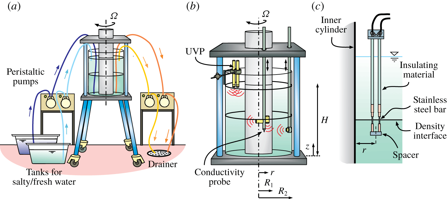
Figure 1. The experimental device. (a) Set-up of the experiments; (b) set-up of the conductivity and UVP probes in the tank; (c) the probe for interface position measurement.
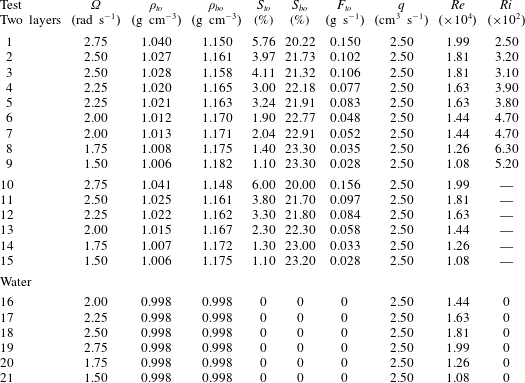
Table 1. Parameters of the experiments. Here  $\unicode[STIX]{x1D6FA}$ is the rotation rate of the inner cylinder; $\unicode[STIX]{x1D70C}_{to}$ and $\unicode[STIX]{x1D70C}_{bo}$ are the density of the top and bottom out-flowing fluid in state-state condition; $S_{to}$ and $S_{bo}$ are the salinity of the top and bottom out-flowing fluid in steady-state condition; $F_{to}$ is the vertical salt flux, measured as $F_{to}=q\unicode[STIX]{x1D70C}_{to}S_{to}$; $q$ is the volume flux of each source/sink; $Re=\unicode[STIX]{x1D714}R_{1}^{2}/\unicode[STIX]{x1D708}$ is the Reynolds number; and $Ri=g(\unicode[STIX]{x1D70C}_{bo}-\unicode[STIX]{x1D70C}_{to})\unicode[STIX]{x1D6EC}/(\unicode[STIX]{x1D70C}_{0}u_{rms}^{2})$ is the Richardson number ( $\unicode[STIX]{x1D70C}_{0}$ is the reference mass density and $\unicode[STIX]{x1D6EC}$ is the integral vertical length scale; see § 3.3).
Density data were recorded by a conductivity probe mounted on a traverse system that profiled the fluid at approximately  $33~\text{s}$ continuously in time (see figure 1b). The probe has two pins (micro USB type B connectors) that work as electrodes spaced ${\approx}0.2~\text{mm}$, with hardware described in Carminati & Luzzatto-Fegiz (Reference Carminati and Luzzatto-Fegiz2017). The volume of measurement is a cylinder of approximate height 0.4 cm and radius 0.2 cm, and the data rate is ${\approx}20~\text{Hz}$. Fluid velocity in the vertical, radial and azimuthal directions was measured by five ultrasound velocity profilers (UVPs; model DOP 2000, Signal Processing SA, Switzerland) with a carrier frequency of 8 MHz and data rate of 15–20 profiles per second, depending on the set-up. The fluid was seeded with $\text{TiO}_{2}$ parcels, characterized by high sonic impedance, so that the UVPs could measure their velocity at different distances (gates) along the axis of the ultrasonic cone on the basis of the Doppler shift of the echoes (see Longo et al. (Reference Longo, Ungarish, Di Federico, Chiapponi and Addona2016) for more details). Because the speed of sound depends on the density and temperature of the fluid, the position of the gate and parcel velocity were corrected using the model for density–bulk modulus–salinity suggested by Mackenzie (Reference Mackenzie1981).
In experiments 1–9 of table 1 the UVP probes were arranged as sketched in figure 1(b), with two probes aligned along the vertical direction (one of them in a fixed position at the middle of the gap, the other one could be manually moved along the radial direction), while the other three probes were aligned along the azimuthal, vertical and radial directions, and they profiled the fluid moving jointly with the conductivity probe.
In experiments 10–15, in order to detect the density perturbations travelling across the interface, a new specific probe, similar to that used in Wessels & Hutter (Reference Wessels and Hutter1996), was custom made with two stainless steel bars 1 mm in diameter, spaced 1 cm apart, exposed to the fluid for a length of 1.8 cm, and insulated along the remainder of the length (see figure 1c). During the experiments, the probe was located so that the mid-section of the exposed length was at the level of the density interface. The distance  $r$ of the probe from the inner cylinder could be varied manually and it was set to $r=2,4,6~\text{cm}$. At each of the three positions the signal was recorded for 20 min at a sampling frequency of ${\approx}20~\text{Hz}$. Other experiments required two of these probes spaced 7 cm in the azimuthal direction, with output signals cross-correlated to estimate the interfacial perturbation phase speed.
Experiments 16–21 were run with homogeneous fluid (fresh water), in order to build a reference for comparison.
Finally, some unpublished data from Petrolo & Woods (Reference Petrolo and Woods2019) are discussed in the present study, in particular in § 4.1, where we deal with shadowgraphy analysis.
2.1 The uncertainty in variables and parameters
The density of the fluid initially filling the tanks was measured with a hydrometer with an accuracy of  $\pm 10^{-3}~\text{g}~\text{cm}^{-3}$. The mass density of the top out-flowing fluid was measured with a refractometer with an accuracy of $\pm 2\times 10^{-3}~\text{g}~\text{cm}^{-3}$. Local and instantaneous mass density of the fluid in the tank during the experiments was measured with a conductivity probe upon calibration, with an overall accuracy of $\pm 3\times 10^{-3}~\text{g}~\text{cm}^{-3}$ also depending on fluid temperature fluctuations. Fluid velocity was measured with an accuracy ${\leqslant}4\,\%$ (Longo et al. Reference Longo, Liang, Chiapponi and Jiménez2012), resulting in a slightly larger uncertainty for the turbulent component ( ${\leqslant}4.5\,\%$) depending on the duration of acquisition for a given bandwidth of ${\approx}20~\text{Hz}$. The relative uncertainty in spectral peak frequency detection is ${\leqslant}2\,\%$. The geometry of the device (internal and external radius) was known with an absolute uncertainty of 0.2 cm. The flow rate of the pumps was known with an uncertainty ${\leqslant}2\,\%$.
The uncertainty of the derived variables has been estimated by adopting the classical error propagation rules, with  $\unicode[STIX]{x0394}Re/Re\leqslant 5\,\%$ and $\unicode[STIX]{x0394}Ri/Ri\leqslant 7\,\%$.
3 Experimental observations and discussion
3.1 The velocity field
The fluid velocity field in the  $z$–
$z$– $r$ plane was reconstructed with an appropriate set-up of the UVP probes. One probe was vertically aligned at a distance $r=0.5$, 1.3, 2, 3, 4, 5, 6, 7 and 8 cm from $R_{1}$, with the head immersed a few millimetres below the free surface of the upper layer and pointing downward. For every position, 6000 profiles were recorded along the vertical direction with a sampling frequency of ${\approx}20~\text{profiles}~\text{s}^{-1}$, a velocity resolution of ${\approx}0.11~\text{cm}~\text{s}^{-1}$ and an axial (with respect to the probe) space resolution of ${\approx}0.03~\text{cm}$.
A second ultrashort UVP probe was radially aligned, with the head at  ${\approx}1~\text{cm}$ from the inner radius of the external cylinder, pointing inward and moving up and down in the vertical direction jointly with the conductivity probe. Also for this second probe, $6000\times 9$ radial velocity profiles were registered, with a sampling frequency of ${\approx}15~\text{profiles}~\text{s}^{-1}$ and an accuracy of ${\approx}0.15~\text{cm}~\text{s}^{-1}$. The total number of UVP profiles for each test is 54 000, which corresponds to a whole number of ${\approx}100$ vertical excursions of the conductivity probe and of the radial probe, considering a time of ${\approx}33$ s for the probes to run the vertical depth $H$ of the fluid.
A typical example of the density profile and time-averaged vertical,  $w$, and radial, $u_{r}$, velocity fields is shown in figure 2(a–c), with data from experiment 1 in table 1, with $\unicode[STIX]{x1D6FA}=2.75~\text{rad}~\text{s}^{-1}$. The interface (density jump) is located at $z\approx 14~\text{cm}$.
Figure 2(b,c) shows the contours of the average vertical and radial velocity, positive upward and outward, respectively. The vectors are the fluid velocity in the  $z$–
$z$– $r$ plane. Blank zones are due to probes moving inside the fluid, and hence occupying a region where data cannot be available, or other geometric limitations. Figure 2(d) shows the instantaneous contour map of the radial velocity, with several recirculation cells not present in the average velocity map, and with a wider velocity range.
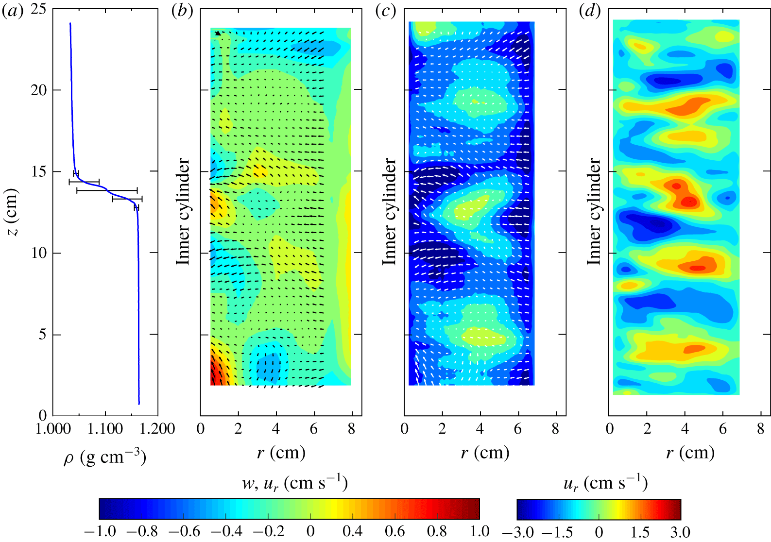
Figure 2. (a) Time-averaged density profile over the period of the steady state, with error bars corresponding to one standard deviation. (b–d) Typical velocity field in the  $z$–
$z$– $r$ plane for a two-layer ambient fluid: (b) contour plot of the time-averaged vertical velocity component, $w$; (c) contour plot of the average and (d) of the instantaneous radial velocity component, $u_{r}$ (positive for outward and negative for inward). The vectors are the time-averaged fluid velocity components. Data refer to experiment 1 of table 1; $\unicode[STIX]{x1D6FA}=2.75~\text{rad}~\text{s}^{-1}$.
The mean vertical velocity contour map exhibits a generally positive value, with a strong exchange of vertical flux at the interface. A red spot of an upward velocity is registered, close to the inner cylinder just below the interface, while a blue spot above the density jump carries fluid downward. A net upward flux is clearly visible at the bottom of the tank, close to the inner cylinder. This is a secondary inward radial flow driven by the centrifugally imbalanced pressure gradient at the bottom boundary, where a no-slip condition holds (Burin et al. Reference Burin, Ji, Schartman, Cutler, Heitzenroeder, Liu, Morris and Raftopolous2006). The mean radial velocity field presents coherent structures, with three persistent main patches of velocity directed towards the outer cylinder (see figure 2c). These features are typical for all the values of rotation rates tested (not shown).
This pattern is visible also for homogeneous fluid in experiment 19 (see figure 3): the parcels move up along the inner cylinder from the bottom of the tank, reaching almost the mid-height of the fluid where they diverge towards the outer cylinder, continuing to move upward. At the free surface, the motion is inverted and parcels start falling along the inner radius for mid-height and deviate to the outer radius. The vertical path is a figure-of-eight shape.
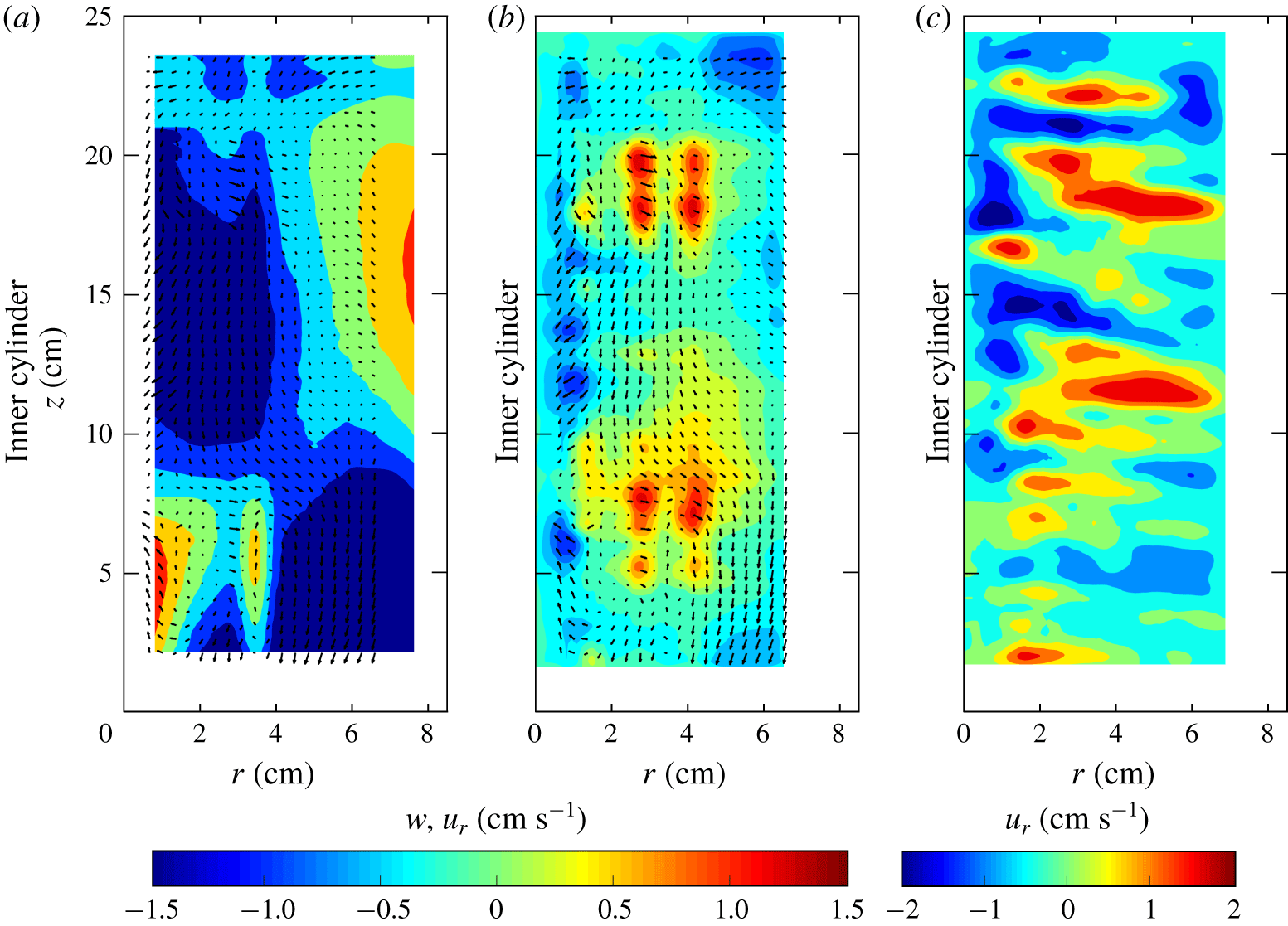
Figure 3. Typical velocity field in the  $z$–
$z$– $r$ plane for water. (a) Contour plot of the time-averaged vertical velocity component, $w$; (b) contour velocity of the time-averaged and (c) of the instantaneous radial velocity component, $u_{r}$, reconstructed by UVP signal from experiment 19 of table 1; $\unicode[STIX]{x1D6FA}=2.75~\text{rad}~\text{s}^{-1}$. The vectors are the time-averaged fluid velocity component.
3.2 The turbulence field
Turbulent velocity fluctuations were extracted by subtracting the instantaneous velocity from the time-averaged velocity. Figure 4 shows the vertical and radial TKE components for two experiments at different  $\unicode[STIX]{x1D6FA}$. Both components are damped near the density interface, and the overall pattern is similar, although with minor intensity for reduced rotation rate. The vertical component dominates near the inner cylinder, with a subsequent diffusion towards the mid-gap and transfer to the radial component.
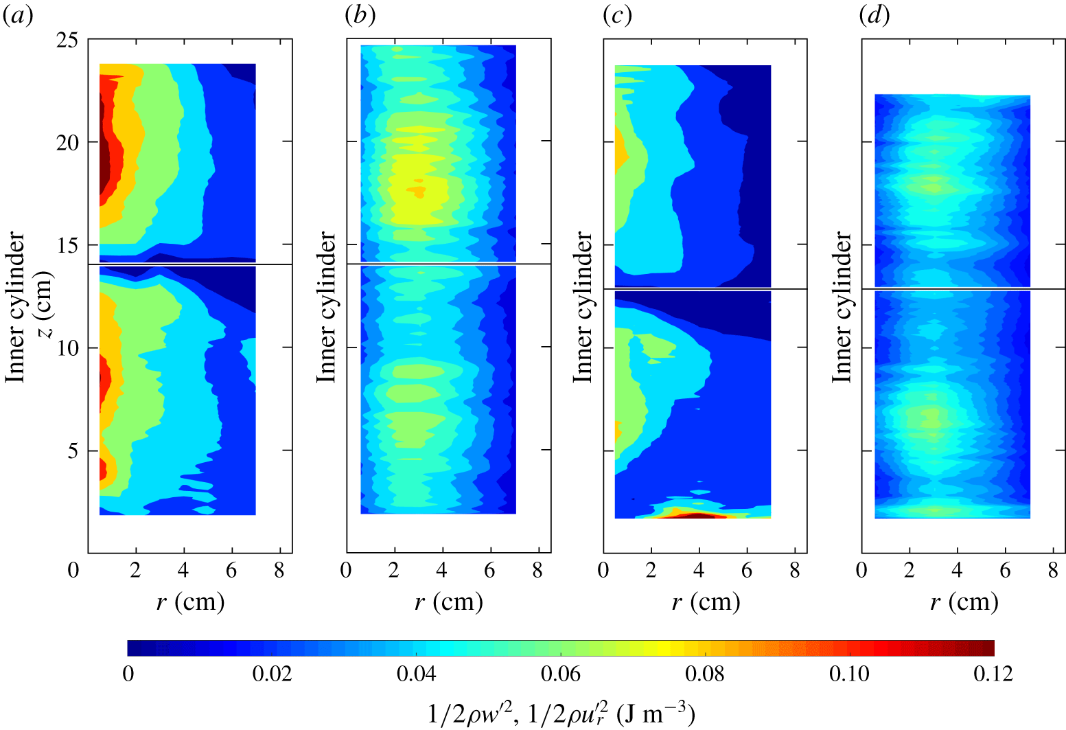
Figure 4. Turbulent kinetic energy. (a) Vertical and (b) radial component for experiment 1;  $\unicode[STIX]{x1D6FA}=2.75~\text{rad}~\text{s}^{-1}$. (c) vertical and (d) radial component for experiment 6; $\unicode[STIX]{x1D6FA}=2.00~\text{rad}~\text{s}^{-1}$. The horizontal line indicates the interface.
Figure 5(a) shows the three components of the TKE and the total value averaged along the total depth of the fluid,  $H$. At low $\unicode[STIX]{x1D6FA}$ (low Reynolds number) the vertical component dominates, followed by the radial component, and the turbulence field is anisotropic. At high $\unicode[STIX]{x1D6FA}$, the three contributions are almost equal and the turbulence field is almost isotropic; at low $\unicode[STIX]{x1D6FA}$ a kink is present that remains unexplained.
We compare the characteristics of our device with those of Woods et al. (Reference Woods, Caulfield, Landel and Kuesters2010), who used a tank with an inner radius of  $R_{1}=10~\text{cm}$ and an outer radius of $R_{2}=25~\text{cm}$, filled with fluid up to a depth $H=40~\text{cm}$. Figure 5(b) shows the fluctuating azimuthal velocity (time-, vertically and gap-averaged) for the different values of Reynolds number $Re=\unicode[STIX]{x1D6FA}R_{1}^{2}/\unicode[STIX]{x1D708}$. The red line represents the empirical relationship
 $$\begin{eqnarray}\langle u_{\unicode[STIX]{x1D703},rms}^{\prime }\rangle _{W10}=\frac{0.086\pm 0.01}{R_{2}-R_{1}}\ln \left(\frac{R_{2}}{R_{1}}\right)\unicode[STIX]{x1D708}Re=(6.3\pm 0.7)\times 10^{-7}Re,\end{eqnarray}$$
 which derives from equation (2.7) of Woods et al. (Reference Woods, Caulfield, Landel and Kuesters2010) ( $\langle u_{rms}^{\prime }r\rangle =(0.086\pm 0.01)\unicode[STIX]{x1D6FA}R_{I}^{2}$), after radial averaging and substituting $\unicode[STIX]{x1D6FA}R_{1}^{2}=\unicode[STIX]{x1D708}Re$. The comparison with the present data interpolation, dashed green line in figure 5(b), shows an adequate superposition although two outliers are evident, with the coefficient $K=0.068\pm 0.01$ instead of $K=0.086\pm 0.01$. This result indicates the scalability of the Taylor–Couette cell as a generator of turbulence.
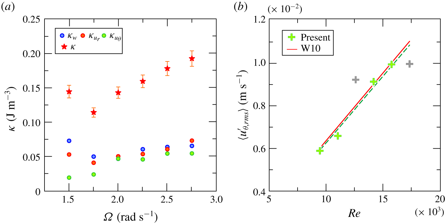
Figure 5. (a) Time- and space-averaged vertical (blue dots), radial (red dots), azimuthal (green dots) and total (red stars) TKE plotted as a function of rotation rate  $\unicode[STIX]{x1D6FA}$. (b) Time-averaged azimuthal fluctuating velocity as a function of $Re$.
$Re$.
3.3 The length scales
The integral,  $\unicode[STIX]{x1D6EC}$, and micro, $\unicode[STIX]{x1D706}$, length scales of the flow field along the three principal directions (vertical, radial and azimuthal) can be evaluated by means of the normalized autocorrelation function of the fluctuating velocity component $\unicode[STIX]{x1D712}(z,\unicode[STIX]{x1D70D})=\overline{u^{\prime }(z,y)u^{\prime }(z,y+\unicode[STIX]{x1D70D})}/\overline{u^{\prime 2}}$, with $u^{\prime }=w^{\prime },u_{r}^{\prime }$ or $u_{\unicode[STIX]{x1D703}}^{\prime }$ and $\unicode[STIX]{x1D70D}$ the space lag. We define the integral length scale $\unicode[STIX]{x1D6EC}(z)=\int _{0}^{\overline{\unicode[STIX]{x1D70D}}}\unicode[STIX]{x1D712}(z,\unicode[STIX]{x1D70D})\,\text{d}\unicode[STIX]{x1D70D}$, where $\overline{\unicode[STIX]{x1D70D}}$ is the length over which the autocorrelation function is positive, while the Taylor micro length scale is related to the curvature of the autocorrelation coefficient at the origin (see Tennekes & Lumley Reference Tennekes and Lumley1972). The integral length scale is representative of the size of the coherent macrostructures of the flow field (large eddies). The Taylor microscale is associated with the small-scale eddies and gives a convenient estimation for the fluctuating strain rate field. In the present analysis we are dealing with Eulerian length scales, since we are considering correlations between fluctuating velocities measured at fixed points in a fixed frame of reference.
Figure 6 shows the vertical, the radial and the azimuthal  $\unicode[STIX]{x1D706}$ and $\unicode[STIX]{x1D6EC}$, with error bands corresponding to one standard deviation, representing the variability within the set of velocity profiles. The general trend is of an increase of the scales with $\unicode[STIX]{x1D6FA}$ and a larger variability in the upper layer with respect to the lower layer. The most relevant variations are observed for the vertical length scales, which drop near the interface at low $\unicode[STIX]{x1D6FA}$. This drop can be related to the interface of thickness $H_{int}$, which, at large values of $Ri=g(\unicode[STIX]{x0394}\unicode[STIX]{x1D70C}/\unicode[STIX]{x1D70C})H_{int}/(\unicode[STIX]{x1D6FA}R_{1})^{2}$, acts like a rigid boundary where the colliding eddies flatten, transferring energy from vertical to horizontal scales (Hannoun et al. Reference Hannoun, Fernando and List1988; Briggs et al. Reference Briggs, Ferziger, Koseff and Monismith1998). The density difference between the layers increases as $\unicode[STIX]{x1D6FA}$ decreases, as the vertical salt transport shows a $\unicode[STIX]{x1D6FA}^{3}$-dependent behaviour (Woods et al. Reference Woods, Caulfield, Landel and Kuesters2010; Petrolo & Woods Reference Petrolo and Woods2019), so $Ri$ increases and the vertical length scales reduce. However, the reduction of energy contained in the vertical is not accompanied by an increase in the $r$–
$r$– $\unicode[STIX]{x1D703}$ plane.
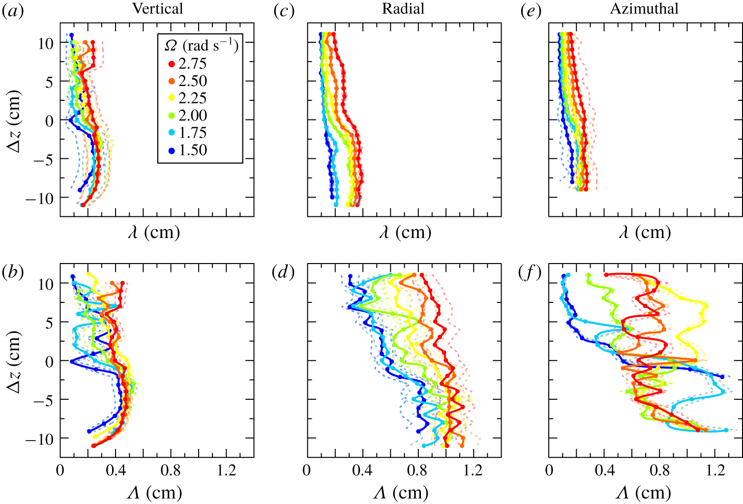
Figure 6. Vertical (a) micro length scales and (b) integral length scales; radial (c) micro length scales and (d) integral length-scales; azimuthal (e) micro length scales and (f) integral length scales as a function of  $z$ for rotation rates $\unicode[STIX]{x1D6FA}=1.50{-}2.75~\text{rad}~\text{s}^{-1}$.
The mean values of the micro length scales in the three directions do not seem to be markedly affected by the interface, as illustrated in figure 6(b,d,f). The micro length scales remain almost isotropic (Fernando Reference Fernando1991), with a mean value  $\unicode[STIX]{x1D706}\approx 0.2\pm 0.1~\text{cm}$. Their values generally decrease with height and $\unicode[STIX]{x1D6FA}$.
The radial and azimuthal  $\unicode[STIX]{x1D6EC}$ are larger than the vertical, with the azimuthal length scale showing a more chaotic trend along the vertical direction and a not-so-evident dependence on $\unicode[STIX]{x1D6FA}$. The eddy geometry is more confined in the vertical than in the radial and azimuthal directions. In these two directions the eddies are quite varying, possibly as a consequence of instabilities of the flow field.
The spatial variations of the three families of length scales are indicative of the role of the interface in forcing the structure of the eddies, mainly at low rotation rate, and of the overall effects of the geometry of the Taylor–Couette cell mainly on the large eddies. The integral length scales in the three directions show a progressive homogeneity for increasing  $\unicode[STIX]{x1D6FA}$.
4 Fluctuations at the interface
4.1 Preliminary visualization of the interface dynamics
A preliminary video image analysis was conducted in order to detect the features of the interface. For an easy visualization, coloured fluids with densities intermediate between those of top and bottom layers were injected by three small pipes at the interface, positioned at three different radial distances from the inner cylinder. These fluids float at the interface before being dispersed in the two layers. A similar analysis was conducted by Oglethorpe (Reference Oglethorpe2014) mainly with the use of shadowgraphy, a technique that will be described later on. Movie 1 is available as https://doi.org/10.1017/jfm.2020.362. Figure 7 shows three snapshots at the early stage of injection of the coloured dye streaks for different  $\unicode[STIX]{x1D6FA}$, with an evident different magnitude of fluctuations at different radial positions and rotation rates.
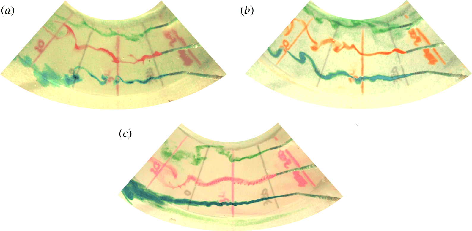
Figure 7. Snapshots of the dye streaks for (a) test at  $\unicode[STIX]{x1D6FA}=2.75~\text{rad}~\text{s}^{-1}$, (b) test at $\unicode[STIX]{x1D6FA}=2.00~\text{rad}~\text{s}^{-1}$ and (c) test at $\unicode[STIX]{x1D6FA}=1.50~\text{rad}~\text{s}^{-1}$. The radial lines are $20^{\circ }$ apart.
A top view obtained with three web cams (not shown) indicates that after an initial chaotic mixing of the dye streaks, a single wave-like perturbation appears (a crest of denser fluid invades the upper layer, eventually a trough of less dense fluid invades the lower layer), generated near the inner cylinder and progressively extending through the gap, with the coloured fluid accumulated behind the front of the perturbation.
Time series of radial lines of pixels are shown in figure 8(a–c) for different  $\unicode[STIX]{x1D6FA}$. The dashed lines mark the inclined fronts of the perturbations corresponding to an outwards excursion of the dye, with a period $T=14{-}23~\text{s}$, decreasing for increasing $\unicode[STIX]{x1D6FA}$. The dyes of three different colours mix and accumulate behind the front, occupying an increasing portion of the interface. It is also evident that the fluctuations of the dye are larger for the green one (the nearest to the inner cylinder) than for the blue one (the nearest to the outer cylinder), and are also increasing for increasing rotation rate. Figure 8(d) shows the time-averaged dye streaks, with an evident correlation of the outwards fluctuations for the green and the red ones. This indicates that the impulse arises near the inner cylinder and propagates radially, although it does not apparently reach the outer cylinder, since the blue streak is much less affected. A more complex scenario is reported in Oglethorpe (Reference Oglethorpe2014), where (i) the strong shear near the inner cylinder favours mixing of fluids, (ii) the mixed fluid travels outwards and generates a bore-like gravity current propagating radially and azimuthally, which (iii) finally spreads in the horizontal plane and in the vertical in both layers. However, the origin and the evolution of the wave-like disturbances are similar in both scenarios, although the events look more energetic in Oglethorpe’s experiments than in the present one. For instance, in the present experiments we could not observe the splash of the fluid on the outer cylinder.
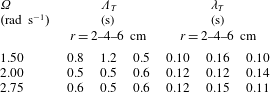
The perturbation dynamics at higher rotation rates is more complex and the perturbation front also includes the blue streaks. The fluctuations are highly self-correlated with a time lag approximately equal to 0.2 s, estimated by digitizing the pixel position and computing the autocorrelation of the signal. The integral and the micro time scales are listed in table 2. The integral time scale decreases for increasing rotation rate and for measurements near the inner cylinder  $r=2~\text{cm}$, indicating that the fluctuations become progressively more random in the region where turbulence is more intense; it remains constant at higher $\unicode[STIX]{x1D6FA}$ for measurements at $r=4{-}6~\text{cm}$. The micro time scales are much less affected by the distance from the inner cylinder and by $\unicode[STIX]{x1D6FA}$, taking an almost constant value.
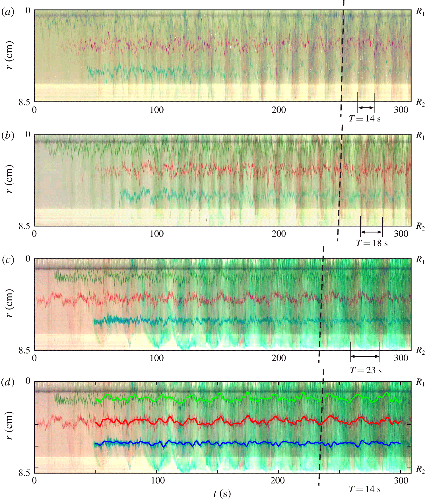
Figure 8. Time series of radial lines of pixels from top-view images: (a)  $\unicode[STIX]{x1D6FA}=2.75~\text{rad}~\text{s}^{-1}$, (b) $\unicode[STIX]{x1D6FA}=2.00~\text{rad}~\text{s}^{-1}$ and (c) $\unicode[STIX]{x1D6FA}=1.50~\text{rad}~\text{s}^{-1}$. (d) Averaged dye streaks for test with $\unicode[STIX]{x1D6FA}=1.50~\text{rad}~\text{s}^{-1}$, moving average with a time window of 3 s. The dashed lines indicate the crest of the perturbation.
Table 2. Integral,  $\unicode[STIX]{x1D6EC}_{T}$, and micro, $\unicode[STIX]{x1D706}_{T}$, time scales measured at distance $r=2$, 4 and 6 cm from the inner cylinder.
Similar information was obtained from a lateral view across the interface. Figure 9 shows three time series (for three different rotation rates) of a vertical line of pixels in false colour across the density interface, where a periodicity is observed. At high rotation rate  $\unicode[STIX]{x1D6FA}=2.75~\text{rad}~\text{s}^{-1}$ (figure 9a), the dye injected at the interface spreads in a vertical wave-like motion and diffuses more rapidly towards the top layer. For this reason, it is not straightforward to detect the periodicity of such perturbations; nevertheless the period $T\approx 14~\text{s}$ has been evaluated as a mean of two subsequent vertical dyed blue stripes. At lower rotation rate $\unicode[STIX]{x1D6FA}=2.00{-}1.50~\text{rad}~\text{s}^{-1}$ (figure 9b,c), the period is equal to $T\approx 19{-}24~\text{s}$, respectively. The enlargement shows a sawtooth profile, with the dye slowly expanding in the advancing disturbance. The different behaviour of the different colours, with cyan beneath the average interface and red mainly above it, is attributed to the different concentrations of the aniline powder, with a consequent slight difference in the density of the coloured fluid.
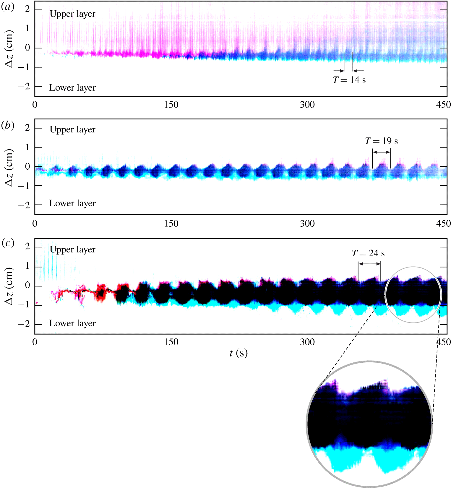
Figure 9. Time series of vertical lines of pixels from lateral-view images: (a)  $\unicode[STIX]{x1D6FA}=2.75~\text{rad}~\text{s}^{-1}$, (b) $\unicode[STIX]{x1D6FA}=2.00~\text{rad}~\text{s}^{-1}$ and (c) $\unicode[STIX]{x1D6FA}=1.50~\text{rad}~\text{s}^{-1}$. The enlargement shows the shape of the perturbation, with a smooth rising front and a steep rear.
A different view is offered by the shadowgraphs shown in figure 10, clearly showing a wake almost symmetric in the two layers with some eddies near the fronts. With the shadowgraph technique, it is possible to visualize any density variation by directing parallel light rays, perpendicularly to the fluid. In our experiments we used a carousel slide projector illuminating horizontally the outer cylinder and projecting shadows created by the density interface and other density variations onto the inner cylinder. We recorded a video with an HD video camera of a mobile phone. Because the tank of the present study had a metallic inner cylinder that reflected most of the light shed by the projector, we chose to show some unpublished data of Petrolo & Woods (Reference Petrolo and Woods2019), who used a tank with a white inner cylinder that made the shadowgraphy analysis much clearer and of higher quality. The wakes observed in the present study were almost identical to those of Petrolo & Woods (Reference Petrolo and Woods2019), with minor insignificant differences. The shadowgraphs of figures 10 and 11 refer to experiment 7 in Petrolo & Woods (Reference Petrolo and Woods2019) and are similar to the wake described in Oglethorpe (Reference Oglethorpe2014). The presence of wakes behind steady breakers at the air–water interface, in the water phase, has been previously detected (see Peregrine & Svendsen Reference Peregrine and Svendsen1978; Battjes & Sakai Reference Battjes and Sakai1981). A steady wake develops also in mixing layers, eventually in presence of fluids of different mass density (Brown & Roshko Reference Brown and Roshko1974). In the present experiments a singular wake develops and diffuses momentum and density upward and downward (see figure 11 where a time series of vertical lines of pixels is extracted from the same experiment shown in figure 10). The wake has a linear increasing transverse length, analogously to the earlier finding of Brown & Roshko (Reference Brown and Roshko1974) for wakes generated by a mixing layer between two fluids of different density; the two fronts delimiting the ambient fluid and the wake expand upward and downward at a speed of approximately  $0.7~\text{cm}~\text{s}^{-1}$ and seem to rebound (at least the front advancing in the upper layer of fluid seems to rebound at the free surface).
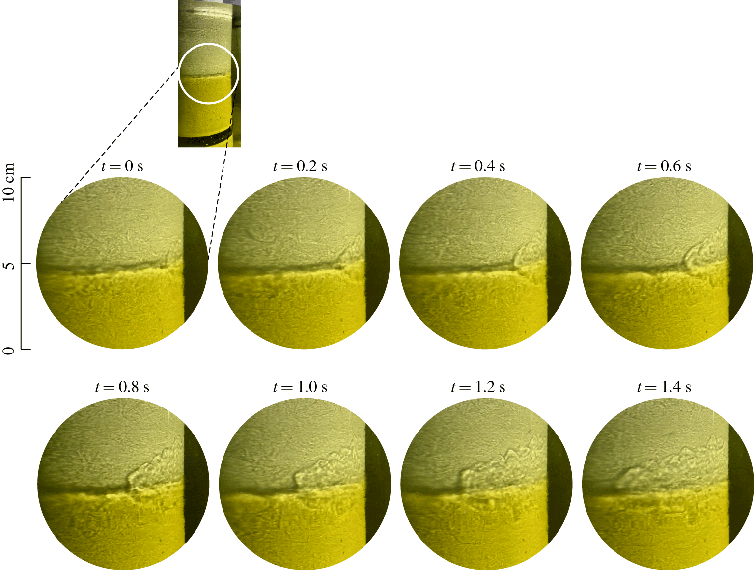
Figure 10. Snapshots of the interface in a two-layer fluid at  $\unicode[STIX]{x1D6FA}=2.50~\text{rad}~\text{s}^{-1}$. Experiment 7 in Petrolo & Woods (Reference Petrolo and Woods2019).
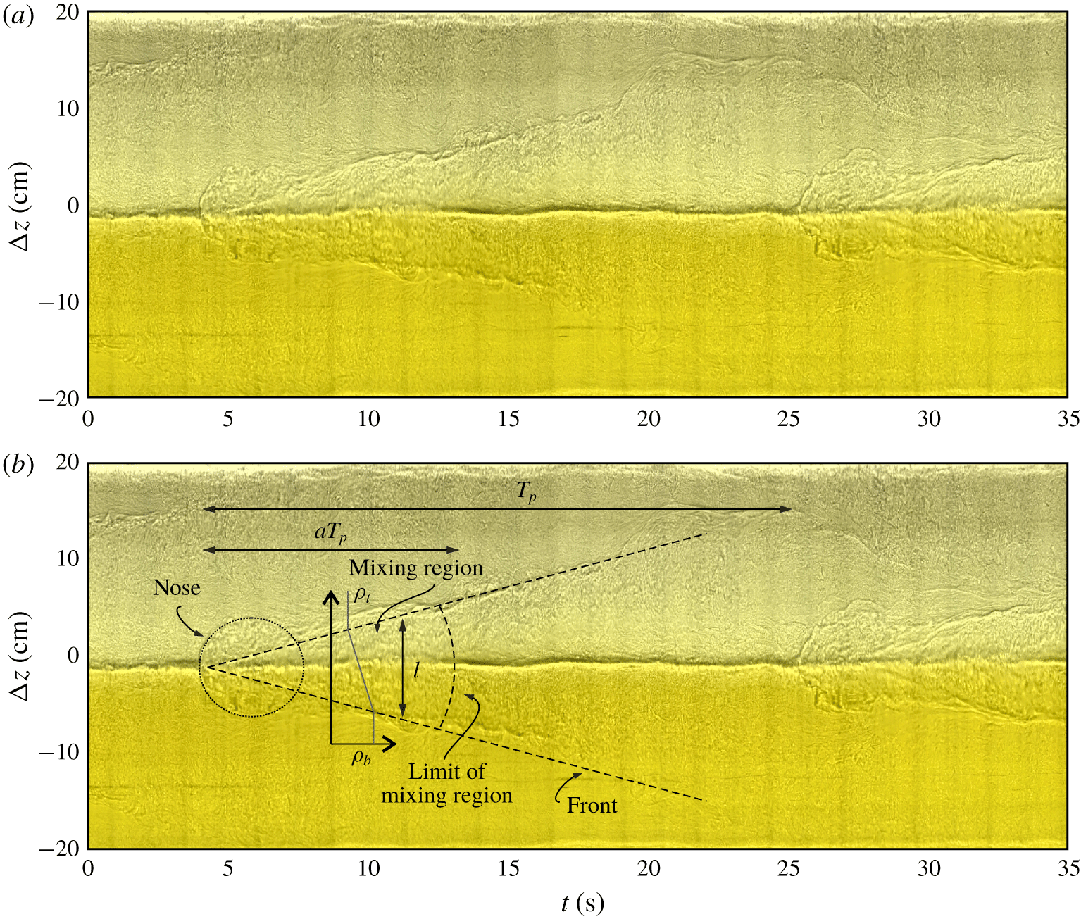
Figure 11. (a) Time series of a vertical line of pixels showing the evolution of the wake expanding from the interface. (b) Sketch of the main features of the wake and schematic for the salt transport model. The slightly different colours indicate the two layers. The dark horizontal band is the interface as evidenced by refraction of the collimated light. Experiment 7 at  $\unicode[STIX]{x1D6FA}=2.50~\text{rad}~\text{s}^{-1}$ in Petrolo & Woods (Reference Petrolo and Woods2019).
The wake enhances mixing and smooths out the sharp density gradient, with a strong diffusion of salt taking place without the singularity of the step density. The disruption of the step density is evident in the nose ( $t\approx 4;25~\text{s}$), where the shadow of the interface is diffused, and persists for several seconds, up to $t\approx 12;32~\text{s}$. The periodicity of the disturbances generates intermittency, with a sequence of low and intense diffusion and with an increasing average value if the disturbances are more frequent. The question remains open as to the source of these wakes and of the mechanism behind the periodicity. A possible explanation (see Singh et al. Reference Singh, Augier, Caulfield, Dalziel, Leclercq and Partridge2018) is a first mode gravity-wave instability forced by a highly turbulent flow at the interface, similar to that observed for a free-surface Taylor–Couette flow (Mujica & Lathrop Reference Mujica and Lathrop2006).
4.2 A model for salt transport
More detailed and quantitative information is given by a series of measurements focused on density and vertical velocity fluctuations across the interface. The conductivity probe and a short UVP probe (connected jointly with the vertical translation bar) acquired the signal for 120 s, moving in steps of 2 mm from one acquisition to the next. The measurement range was  $\pm 2~\text{cm}$ relative to the average position of the interface. Figure 12(a,b) shows the fluctuating density and fluctuating vertical velocity (root-mean-square values). The thickness of the interface $h_{interface}\approx 1~\text{cm}$ is estimated by the range of $\unicode[STIX]{x0394}z$ corresponding to 80 % of the cumulated area of the $\unicode[STIX]{x1D70C}_{rms}^{\prime }$ curve. At the density discontinuity, $\unicode[STIX]{x1D70C}_{rms}^{\prime }$ grows rapidly, whereas $w_{rms}^{\prime }$ decreases towards the interface more gradually, approaching zero at lower $\unicode[STIX]{x1D6FA}$. Figure 12(c) shows the correlation of the two fluctuating variables, with positive peaks near the interface, more localized at intermediate $\unicode[STIX]{x1D6FA}$ and spreading over a wider range if the rotation rate increases (equivalent to increasing $Re$). The vertical average value of $\overline{\unicode[STIX]{x1D70C}^{\prime }w^{\prime }}$ across the interface within the vertical interval comprising 98 % of the cumulated correlation across the interface, referred to a 4 cm window, can be interpreted as the vertical buoyancy flux per unit area. If we compare it with the buoyancy flux estimated as $B_{m}=q\unicode[STIX]{x1D70C}_{to}S_{to}g/\unicode[STIX]{x1D70C}_{0}=F_{to}g/\unicode[STIX]{x1D70C}_{0}$, where $\unicode[STIX]{x1D70C}_{to}$ and $S_{to}$ are the mass density and salinity of the upper out-flowing fluid and $F_{to}\equiv q\unicode[STIX]{x1D70C}_{to}S_{to}$ is the salt flux measured as mass of salt per unit of time (see figure 12d), we find an adequate overlap. The vertical buoyancy flux shows a $B_{m}\sim \unicode[STIX]{x1D6FA}^{3}$ dependence, as previously found by Woods et al. (Reference Woods, Caulfield, Landel and Kuesters2010) and Petrolo & Woods (Reference Petrolo and Woods2019), and vanishes at low $\unicode[STIX]{x1D6FA}$.
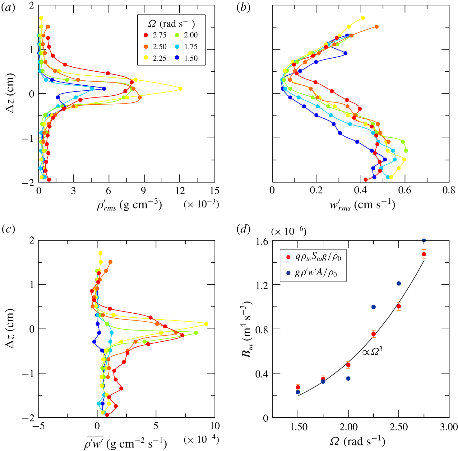
Figure 12. Detailed measurements across the interface. (a) Density fluctuations. (b) Vertical velocity fluctuations. (c) Correlation between density and vertical velocity fluctuations. (d) Comparison between the buoyancy flux measured as the integral vertical salt transport and salt transport across the density interface.
In order to model the effect of the wake on salt transport, we assume that at a given azimuthal position the wake has a transverse length scale  $l(t)$ (see figure 11b) and a linear density variation with a uniform vertical gradient of density equal to $(\unicode[STIX]{x1D70C}_{t}-\unicode[STIX]{x1D70C}_{b})/l(t)$, with a vertically invariant correlation in the mixing region modelled as
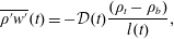 $$\begin{eqnarray}\overline{\unicode[STIX]{x1D70C}^{\prime }w^{\prime }}(t)=-{\mathcal{D}}(t)\frac{(\unicode[STIX]{x1D70C}_{t}-\unicode[STIX]{x1D70C}_{b})}{l(t)},\end{eqnarray}$$
 where  ${\mathcal{D}}(t)$ is the mass diffusivity. We assume that diffusion is relevant for a fraction $\unicode[STIX]{x1D6FC}T_{p}$ of the period of the wake (the mixing region in figure 11(b), where the mixing region was estimated by eye as limited by the nose and by the section where the interface gets ‘darker’ again after disruption), with an average vertical flux over a cycle equal to
 $$\begin{eqnarray}\frac{1}{T_{p}}\int _{t_{0}}^{t_{0}+\unicode[STIX]{x1D6FC}T_{p}}\overline{\unicode[STIX]{x1D70C}^{\prime }w^{\prime }}\,\text{d}t=-\frac{1}{T_{p}}\int _{t_{0}}^{t_{0}+\unicode[STIX]{x1D6FC}T_{p}}{\mathcal{D}}(t)\frac{(\unicode[STIX]{x1D70C}_{t}-\unicode[STIX]{x1D70C}_{b})}{l(t)}\,\text{d}t\equiv \frac{F_{t0}}{A},\end{eqnarray}$$
 where  $A$ is the cross-section of the tank. By assuming a diffusivity ${\mathcal{D}}(t)=k_{\unicode[STIX]{x1D70C}}l(t)c$, where $k_{\unicode[STIX]{x1D70C}}$ is a coefficient and $c$ is the speed of the wake (the velocity scale, see § 4.4), equation (4.2) yields
 $$\begin{eqnarray}k_{\unicode[STIX]{x1D70C}}\unicode[STIX]{x1D6FC}=\frac{F_{to}}{A(\unicode[STIX]{x1D70C}_{b}-\unicode[STIX]{x1D70C}_{t})c}.\end{eqnarray}$$
 Figure 13 shows the experimental value of  $k_{\unicode[STIX]{x1D70C}}\unicode[STIX]{x1D6FC}$ for increasing $\unicode[STIX]{x1D6FA}$, which attains a fairly constant value equal to $1.4\times 10^{-3}\pm 8\,\%$. For the experiment in figure 11, the results are $\unicode[STIX]{x1D6FC}\approx 0.4$ and $k_{\unicode[STIX]{x1D70C}}=0.0035$. In order to compare this result with the coefficient of the Prandtl model (Prandtl Reference Prandtl1942), we keep in mind that the Schmidt number for the diffusivity of the mass, defined as $Sc\equiv \unicode[STIX]{x1D708}_{T}/{\mathcal{D}}$, can be extremely variable, generally differs from unity (Brown & Roshko Reference Brown and Roshko1974; Variano & Cowen Reference Variano and Cowen2013) and has an important role in mixing processes (Leclercq et al. Reference Leclercq, Partridge, Augier, Caulfield, Dalziel and Linden2016a,Reference Leclercq, Partridge, Augier, Caulfield, Dalziel and Lindenb). By assuming for simplicity that $Sc=1$ the empirical proportionality coefficient for the flux of momentum is $k_{T}=k_{\unicode[STIX]{x1D70C}}$, which is slightly less than the coefficient of Prandtl for plane mixing layers, $k_{T,Prandtl}=0.01$. The difference is related to the velocity scale, here assumed for simplicity equal to the speed of the wake and that should more correctly be related to the defect of velocity in the mixing layer (e.g. Tennekes & Lumley Reference Tennekes and Lumley1972). We also neglected the entrainment and the region of the nose, characterized by a more complex scenario, and we have also pragmatically assumed that the structure of the wake is radially invariant.
Figure 13. Coefficient  $k_{\unicode[STIX]{x1D70C}}\unicode[STIX]{x1D6FC}$ relating the average diffusivity to the length and velocity scales.
4.3 Quadrant analysis
The fluctuating density and vertical velocity correlation was also analysed with a quadrant decomposition (e.g. Variano & Cowen Reference Variano and Cowen2013), with a conditional sampling of the events belonging to the first quadrant ( $\unicode[STIX]{x1D70C}^{\prime }>0,w^{\prime }>0$), to the second quadrant ( $\unicode[STIX]{x1D70C}^{\prime }<0,w^{\prime }>0$), to the third quadrant ( $\unicode[STIX]{x1D70C}^{\prime }<0,w^{\prime }<0$) and to the fourth quadrant ( $\unicode[STIX]{x1D70C}^{\prime }>0,w^{\prime }<0$). Figure 14 shows a schematic diagram depicting the events that control vertical transport of salt near the interface. Since the vertical density gradient is negative, the diffusive flux belongs to Q1 and Q3; the contra-diffusive flux belongs to Q2 and Q4.
A similar schematic is depicted in Odier, Chen & Ecke (Reference Odier, Chen and Ecke2012), where entrainment (detrainment) is defined when a parcel of fluid that is lighter (heavier) is advected into (out of) the current and thoroughly mixed. However, the model in Odier et al. (Reference Odier, Chen and Ecke2012) refers to a gravity turbulent current advancing in a homogeneous domain of fluid mainly at rest, whereas in the present experiments turbulence is present in both layers.
Figure 14. Schematic diagram showing the eddies carrying excess or deficit of density: Q1 ( $\unicode[STIX]{x1D70C}^{\prime }>0,w^{\prime }>0$), Q2 ( $\unicode[STIX]{x1D70C}^{\prime }<0,w^{\prime }>0$), Q3 ( $\unicode[STIX]{x1D70C}^{\prime }<0,w^{\prime }<0$), Q4 ( $\unicode[STIX]{x1D70C}^{\prime }>0,w^{\prime }<0$). The horizontal arrows indicate that part of the action of Q3 (Q1) is transferred to Q2 (Q4). Here $\text{Q}1+\text{Q}3$ is the diffusive action, $\text{Q}2+\text{Q}4$ is the contra-diffusive action.
The event-averaged (phase-averaged) contribution of the  $i$th quadrant is
 $$\begin{eqnarray}\langle \overline{\unicode[STIX]{x1D70C}^{\prime }w^{\prime }}\rangle _{i}=\frac{1}{N_{i}}\mathop{\sum }_{j=1}^{N_{i}}[(\unicode[STIX]{x1D70C}^{\prime }w^{\prime })_{j}]_{i}\quad \text{for }i=1,\ldots 4,\end{eqnarray}$$
 where  $N_{i}$ is the number of events in the $i$th quadrant. The time-averaged contribution of the $i$th quadrant is
 $$\begin{eqnarray}(\overline{\unicode[STIX]{x1D70C}^{\prime }w^{\prime }})_{i}=\frac{1}{N}\mathop{\sum }_{j=1}^{N_{i}}[(\unicode[STIX]{x1D70C}^{\prime }w^{\prime })_{j}]_{i}\quad \text{for }i=1,\ldots 4,\end{eqnarray}$$
 where  $N$ is the total number of events for all quadrants. Here $N_{i}/N$ is the time of permanence (concentration) of events in the $i$th quadrant, hence
 $$\begin{eqnarray}(\overline{\unicode[STIX]{x1D70C}^{\prime }w^{\prime }})_{i}=\frac{N_{i}}{N}\langle \overline{\unicode[STIX]{x1D70C}^{\prime }w^{\prime }}\rangle _{i},\quad \text{with }\overline{\unicode[STIX]{x1D70C}^{\prime }w^{\prime }}=\mathop{\sum }_{i=1}^{4}(\overline{\unicode[STIX]{x1D70C}^{\prime }w^{\prime }})_{i}.\end{eqnarray}$$
We can also analyse the events over a threshold, selecting only the correlation terms satisfying the relation
 $$\begin{eqnarray}|\unicode[STIX]{x1D70C}^{\prime }w^{\prime }|>\unicode[STIX]{x1D6FD}Th\equiv \unicode[STIX]{x1D6FD}(\unicode[STIX]{x1D70C}_{rms}^{\prime }w_{rms}^{\prime }),\end{eqnarray}$$
 where  $\unicode[STIX]{x1D6FD}$ is a coefficient of a threshold $Th$ assumed equal to the product of the root-mean-square values of density and vertical velocity fluctuations (a different scale can be selected).
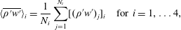
Figure 15 shows the concentration and the time- and phase-average quadrant contribution (no threshold, with  $\unicode[STIX]{x1D6FD}=0$) to the salt flux $\overline{\unicode[STIX]{x1D70C}^{\prime }w^{\prime }}$ for experiment 1, with positive contribution (upward flux) from quadrants 1–3 and negative contribution from quadrants 2–4, with the latter approximately half the value of the former. The average salt flux is positive, as expected, as a result of the dominant contribution of diffusive terms, almost equally distributed among quadrants 1–3. The intensity of the events, represented by the phase-average values, is stronger from quadrant 3, i.e. the lighter fluid of the upper layer sinking into the lower and denser one; these events have a time concentration generally lower than the other three quadrants, so they are not so frequent events but they are quite strong. The time-average peak value is ${\approx}0.6$, which decays to ${\approx}0.1$ at distance of $\unicode[STIX]{x0394}z=0.5~\text{cm}$.
Figure 16 shows the same data as in figure 15 for  $\unicode[STIX]{x1D6FD}=2$. The intense events are much less frequent and are non-zero only near the interface. Phase-averaged contributions of the four quadrants are generally more balanced, with events having comparable intensity for all quadrants, being more frequent for quadrants 1–3, with a dominance of quadrant 3 ( $\unicode[STIX]{x1D70C}^{\prime }<0,w^{\prime }<0$), revealing that the bursts of lighter fluid parcels downward are intense and frequent. According to this scheme, the (diffusive) action generating salt flux is turbulence in the upper layer, with lighter fluid eddies scraping the interface from the top. More than 60 % of the flux is related to these energetic events (the dimensionless value of the peak at the interface is equal to ${\approx}0.4$, whereas the corresponding values for all events equal ${\approx}0.6$). This analysis confirms that the flux of buoyancy is an intermittent phenomenon also at the small scale, with intense events occurring immediately after the passage of the wave-like perturbation described in § 4.1, although we do not have enough data to check it. However, we bear in mind that our measurements refer to a single radial position and that the scenario could be radially heterogeneous.
Figure 15. Cross-correlation of fluctuating density and vertical velocity, with conditional values from each quadrant, no threshold ( $\unicode[STIX]{x1D6FD}=0$). (a) Concentration. (b) Time-average correlation computed according to (4.5). (c) Phase-average correlation computed according to (4.6). Filled circles indicate the contribution from all quadrants, Q1 ( $\unicode[STIX]{x1D70C}^{\prime }>0,w^{\prime }>0$), Q2 ( $\unicode[STIX]{x1D70C}^{\prime }<0,w^{\prime }>0$), Q3 ( $\unicode[STIX]{x1D70C}^{\prime }<0,w^{\prime }<0$), Q4 ( $\unicode[STIX]{x1D70C}^{\prime }>0,w^{\prime }<0$). Data from experiment 1; $\unicode[STIX]{x1D6FA}=2.50~\text{rad}~\text{s}^{-1}$.
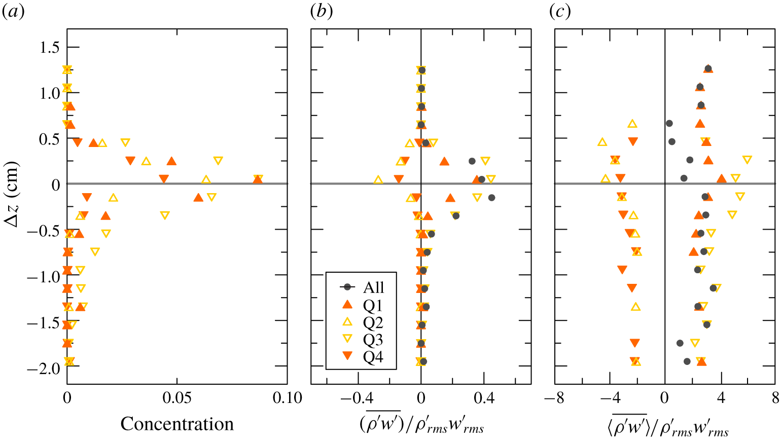
Figure 16. Cross-correlation of fluctuating density and vertical velocity, with conditional values from each quadrant and with  $\unicode[STIX]{x1D6FD}=2$. For details, see caption to figure 15.
Figure 17 shows the joint probability density functions for the events in the four quadrants, and figure 18 shows the contribution of each quadrant to the flux. This figure confirms the results of the quadrant analysis. We observe that in the upper layer negative density fluctuations are frequently characterized by negative vertical velocity fluctuations, i.e. lighter fluid descends into the denser and lower layer; in the lower layer, near the interface, there is an evident dominance of heavy fluid parcels moving preferentially upward. Below the interface the contribution of quadrant 1 is dominant; above the interface the most relevant contribution is due to quadrant 3.
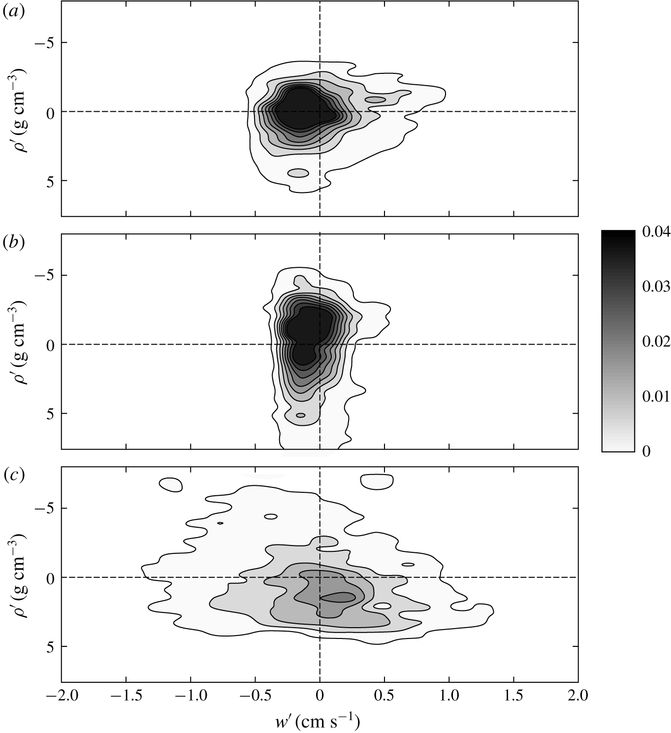
Figure 17. Joint probability density function of  $w^{\prime }$ and $\unicode[STIX]{x1D70C}^{\prime }$: (a) $\unicode[STIX]{x0394}z=0.85~\text{cm}$, (b) $\unicode[STIX]{x0394}z=0.65~\text{cm}$ and (c) $\unicode[STIX]{x0394}z=-0.35~\text{cm}$.
Figure 18. Frequency-weighted turbulent flux absolute value: (a)  $\unicode[STIX]{x0394}z=0.85~\text{cm}$, (b) $\unicode[STIX]{x0394}z=0.65~\text{cm}$ and (c) $\unicode[STIX]{x0394}z=-0.35~\text{cm}$.
4.4 The dynamics at the interface
In order to quantify the interface fluctuations, a twin-wire conductivity probe was assembled and connected to mainly the same electronics as was the density probe, and was calibrated by recording the conductivity of the quiescent two-layer fluid at different vertical positions with respect to the interface. The probe proved extremely sensitive and stable, with an overall accuracy better than  $0.1~\text{mm}$ and a frequency response of a few hertz. The recorded time series lasting for 10 min showed a drift of the average level of the interface up to ${\approx}1~\text{mm}$, which is mainly attributed to small imbalances of the peristaltic pumps. Figure 19(a) shows a time window of the raw signal (after de-trending), $\unicode[STIX]{x1D702}$, and of the moving-average signal of the interface position for experiment 10, run at $\unicode[STIX]{x1D6FA}=2.75~\text{rad}~\text{s}^{-1}$. A sequence of waves is observed, further analysed in the time domain with a zero (up)crossing method. The average wave height of the highest third of the waves (trough to crest; see e.g. Goda (Reference Goda2010)) and period of the waves are $H_{w,1/3}\approx 0.7~\text{mm}$ and $T_{1/3}\approx 15~\text{s}$, respectively. Period $T_{1/3}$ does not change dramatically with $\unicode[STIX]{x1D6FA}$, and reaches a peak of ${\approx}18~\text{s}$ at $\unicode[STIX]{x1D6FA}=2.00~\text{rad}~\text{s}^{-1}$ and a lowest value of ${\approx}12~\text{s}$ at $\unicode[STIX]{x1D6FA}=1.50~\text{rad}~\text{s}^{-1}$. On the other hand, $H_{w,1/3}$ decreases monotonically with $\unicode[STIX]{x1D6FA}$, reaching $H_{w,1/3}=0.2$ mm at $\unicode[STIX]{x1D6FA}=1.50~\text{rad}~\text{s}^{-1}$. Similar data can be retrieved in the frequency domain, observing the spectra showing peaks in correspondence of the waves (see figure 19b). We notice that the measured height of these fluctuations is much lower than that estimated in Oglethorpe (Reference Oglethorpe2014), where particle image velocimetry measurements suggested a value of less than 2 cm. Figure 20 shows the peak period of the interfacial disturbances computed from the spectra as a function of $\unicode[STIX]{x1D6FA}$. While near the inner cylinder ( $r=2~\text{cm}$) the peak period of the waves is strongly varying, without a specific trend except at high $\unicode[STIX]{x1D6FA}$, in the mid-gap and near the outer cylinder positions ( $r=4{-}6~\text{cm}$) the period is $T_{p}\propto \unicode[STIX]{x1D6FA}^{-1}$, and is radially homogeneous. This behaviour indicates that for $\unicode[STIX]{x1D6FA}<2.00~\text{rad}~\text{s}^{-1}$ the disturbances, generated near the inner cylinder (the ‘fetch’ in the context of wind gravity waves), propagate outward and coalesce with a nonlinear interaction, doubling the period and finally attaining a regime configuration. For $\unicode[STIX]{x1D6FA}>2~\text{rad}~\text{s}^{-1}$ the evolution of the perturbations is much faster and the regime configuration is obtained even at $r=2~\text{cm}$. The continuous curve is the interpolating function $T_{p}=12\unicode[STIX]{x03C0}/\unicode[STIX]{x1D6FA}$ (frequency peak of the disturbances equal to $1/6$ of the frequency of rotation). The experiments in Oglethorpe (Reference Oglethorpe2014) suggested $T=4.82\sqrt{(R_{2}-R_{1})/R_{1}}(2\unicode[STIX]{x03C0}/\unicode[STIX]{x1D6FA})$, which, for the present experimental configuration, gives $9.75\unicode[STIX]{x03C0}/\unicode[STIX]{x1D6FA}$. There is no clear explanation for the differences, although the analysis given in Mujica & Lathrop (Reference Mujica and Lathrop2006) for a free-surface Taylor–Couette flow shows that bistability and hysteresis are observed, with an azimuthal pattern related to the mean flow and free surface.
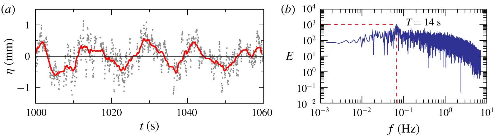
Figure 19. (a) Interface position for experiment 10. Raw signal after de-trending (grey dots) and moving average with a time window of  ${\approx}2.5~\text{s}$ (red line). The time origin is the start of the record. (b) Energy spectrum in the frequency domain for experiment 10.
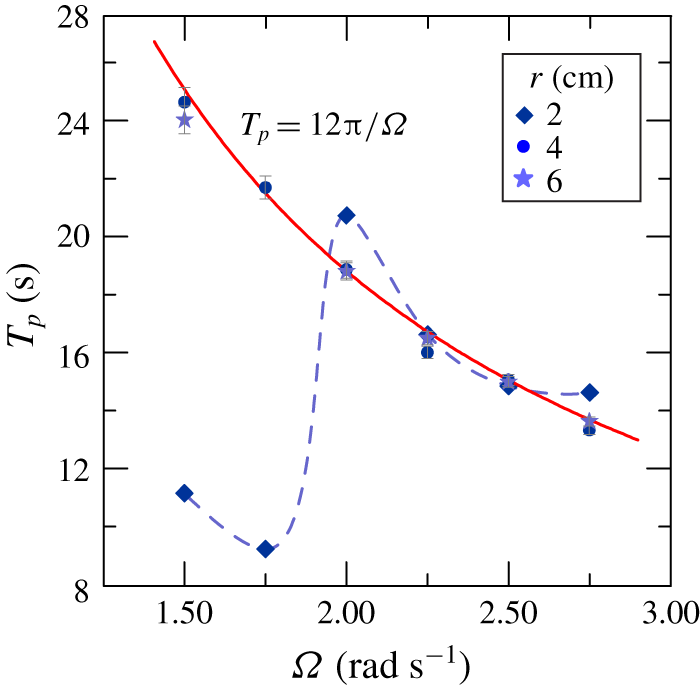
Figure 20. Experimental peak period (symbols) of the interfacial disturbances measured from the spectra at different radial positions as a function of  $\unicode[STIX]{x1D6FA}$. The dashed curve connects measurements near the inner cylinder; the continuous curve is the interpolating curve $T_{p}=12\unicode[STIX]{x03C0}/\unicode[STIX]{x1D6FA}$.
In order to underpin the nature of these perturbations, we assume that some part of the kinetic energy of a fluid element is transformed into potential energy (see also Boubnov et al. (Reference Boubnov, Gledzer and Hopfinger1995) for a similar approach).
The potential energy per unit area of the interface of the wave-like perturbations is equal to
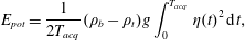 $$\begin{eqnarray}E_{pot}=\frac{1}{2T_{acq}}(\unicode[STIX]{x1D70C}_{b}-\unicode[STIX]{x1D70C}_{t})g\int _{0}^{T_{acq}}\unicode[STIX]{x1D702}(t)^{2}\,\text{d}t,\end{eqnarray}$$
 where  $T_{acq}$ is the duration of the acquisition. Figure 21(a) shows the time- and radially averaged TKE as a function of the height of the fluid, and it refers to the same experiment as that of figure 2. From the steady-state density profile reported in figure 2(a), we can see that a sharp density interface is present at $z=12.5{-}15~\text{cm}$. This interface determines a local TKE reduction, as shown in figure 21(a). As a pragmatic definition, we define the shaded area as the ‘missing TKE’, $\text{TKE}_{mis}$, which is energy by unit surface, and represents the TKE that we assume can be transformed into energy stored in the wave-like perturbations. Energy $\text{TKE}_{mis}$ can be decomposed into the three components due to the radial ( $r$-component), vertical ( $z$-component) and azimuthal ( $\unicode[STIX]{x1D703}$-component) velocity fluctuations, including their combinations.
Figure 21(b) shows the average potential energy from (4.8) as a function of  $\text{TKE}_{mis}$, with three different series referred to as only the vertical velocity fluctuations $w^{\prime }$ (blue dots), to the vertical and radial velocity fluctuations, $w^{\prime }$ and $u_{r}^{\prime }$ (orange dots), and to all three components of the velocity fluctuations (green dots). Energy $\text{TKE}_{mis}$ increases with rotation rate at low rotation rate, before reaching a plateau for $\unicode[STIX]{x1D6FA}>2.25~\text{rad}~\text{s}^{-1}$. In all the experiments the potential energy of the interface fluctuations is only a few percent of the missing TKE, and even if we could evaluate the total energy of the fluctuations by adding the kinetic energy of the wave-induced velocity (not measured in the present tests, but of the same order as the potential energy – equal to the potential energy for linear waves), it still would be a small amount of the missing TKE. For $\unicode[STIX]{x1D6FA}>2.25~\text{rad}~\text{s}^{-1}$, when turbulence becomes very intense, the missing TKE reaches a plateau as an indication of the progressive reduction of the difference between the density of the top and bottom layers in steady state. With increasing $\unicode[STIX]{x1D6FA}$, the density contrast between the layers becomes so small that it can be overturned by turbulence. Therefore, the fluid evolves towards a weak stratification and eventually, with a further increase in $\unicode[STIX]{x1D6FA}$, towards a well-mixed condition. The contribution of the vertical velocity fluctuations to missing TKE disappears for $\unicode[STIX]{x1D6FA}>2.75~\text{rad}~\text{s}^{-1}$. In fact, experiments run at $\unicode[STIX]{x1D6FA}=3.00~\text{rad}~\text{s}^{-1}$ (not presented) show that the interface is eroded by turbulent eddies and gradually disappears and the initial two-layer fluid evolves towards a linearly stratified fluid, with a completely different scenario. Because no density interfaces are present when the fluid becomes linearly stratified, there is no discontinuous profile of TKE, and it is no longer possible to detect the ‘missing TKE’.
Figure 21. (a) The time- and radially averaged TKE profile for experiment 1 in table 1, with the shaded area representing the ‘missing TKE’. (b) Potential energy of the density interface as a function of the missing TKE, evaluated as a function of only the vertical (blue dots), vertical and radial (orange dots) and the three components (green dots) of the fluctuating velocity.
Another study of interest is a comparison between the phase speed of the interfacial disturbances and the speed of the coherent structures, in order to analyse how these two quantities of the flow field are related. The phase speed  $c$ of the interfacial perturbations was estimated by correlating the signals of two twin-wire conductivity probes located at $r=3~\text{cm}$ (with the two wires radially aligned) and spaced $\unicode[STIX]{x1D6E5}=7~\text{cm}$ in the azimuthal direction, and measuring the time delay of the peak $\unicode[STIX]{x1D70F}_{p}$, with $c=\unicode[STIX]{x1D6E5}/\unicode[STIX]{x1D70F}_{p}$. The estimation of the speed of the coherent structures required a final series of measurements with two UVP probes pointing downward located at $r=3.5~\text{cm}$ and separated by $3.5~\text{cm}$ azimuthally, recording the vertical velocity over the depth of both top and bottom layers of fluid. A number of 2000 velocity profiles were recorded by each probe in multiplexing with a frequency of 10 couples of profiles per second. Figure 22 shows the typical pattern for high and low $\unicode[STIX]{x1D6FA}$, with the line at $\unicode[STIX]{x0394}z=0$ marking the position of the density interface. The experiment with $\unicode[STIX]{x1D6FA}=1.50~\text{rad}~\text{s}^{-1}$ has peaks only in the upper layer (not shown) whilst higher values of $\unicode[STIX]{x1D6FA}$ show evident peaks in the correlation in both layers. The peak of the correlation has a time delay equal to the time of travel of the coherent structures and allows for the computation of the speed of these structures. Since there is a limited variability in the vertical, we consider the average speed.
Figure 22. Cross-correlation map of vertical velocities in the time domain for two UVP probes at  $r=3.5~\text{cm}$ and $3.5~\text{cm}$ apart in the azimuthal direction. (a) Experiment 1 with $\unicode[STIX]{x1D6FA}=2.75~\text{rad}~\text{s}^{-1}$. (b) Experiment 8 with $\unicode[STIX]{x1D6FA}=1.75~\text{rad}~\text{s}^{-1}$. The lines at $\unicode[STIX]{x0394}z=0$ indicate the density interface.
Figure 23 shows the speed of the interfacial perturbations and the speed of the coherent structures. Both values increase for increasing  $\unicode[STIX]{x1D6FA}$ with coherent structures generally slower than the interfacial perturbations, with a decreasing difference for increasing $\unicode[STIX]{x1D6FA}$. The different values of the speed of coherent structures and speed of interfacial perturbations suggest that the dynamics of the two processes is controlled by different factors, with the velocity lag favouring mixing at the interface. A possible resonance is forecast for $\unicode[STIX]{x1D6FA}>2.75~\text{rad}~\text{s}^{-1}$, if the celerities become equal. In fact experiments at $\unicode[STIX]{x1D6FA}=3.00~\text{rad}~\text{s}^{-1}$ (not shown) indicate that, for the given buoyancy supplied at the base, the two-layer stratification evolves towards a linear stratification.
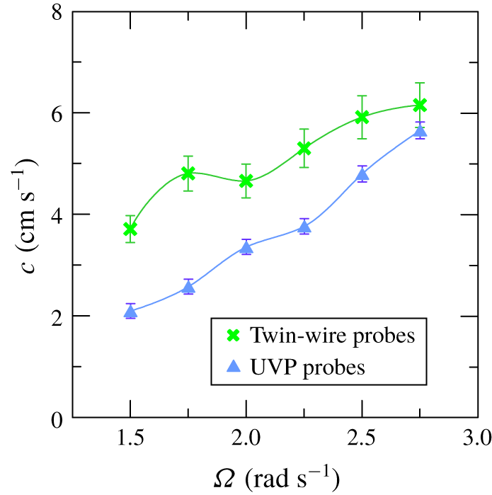
Figure 23. Speed of the interfacial perturbations (crosses) at  $r=3~\text{cm}$ and of the coherent structures (triangles) at $r=3.5~\text{cm}$. Error bars are one standard deviation.
5 Conclusion
Our experiments focused on the mechanisms of turbulent transport in a two-layer fluid in a non-invasive turbulence generator, a Taylor–Couette tank. In our experiments, we stabilized the density interface with a source of fresh water and salty water at the top and bottom of the tank, respectively. At the same time we withdrew the same volume flux as the supply by two sinks positioned at the same depths as the respective sources.
The fluid velocity was measured with UVPs. The average vertical velocity contour maps show a variegate pattern, with some recirculation cells that are affected by the two-layer configuration. A strong exchange of fluid occurs at the interface, near the inner cylinder, and a more in-depth analysis reveals that the interface is indeed affected by multiple complex mechanisms. Similar complexity is shown in the contour maps of the radial velocity, also characterized by a significant variation in time with (almost) instantaneous snapshots different from the time-average distribution. Outward and inward fluxes alternate in the vertical, with persistent cells, with an average velocity less than  $1~\text{cm}~\text{s}^{-1}$ but with short-time velocity up to $3~\text{cm}~\text{s}^{-1}$. Similar contour maps for the TKE components indicate higher energy near the inner cylinder, damped at the interface and radially spread. The turbulent field is anisotropic near the inner cylinder and progressively becomes isotropic and homogeneous, except at the interface. This is an indicator of the complex interaction of TKE and buoyancy flux. The overall mechanism of salt transport is not steady, and periodic disturbances develop and travel at the interface, with corresponding slower coherent structures propagating in the azimuthal direction.
A first preliminary analysis of the video image from the side of the tank showed that the disturbances (waves) are generated regularly and periodically near the inner cylinder and propagate progressively in the radial and azimuthal directions. Video 2 is available as supplementary material. The videos from above confirmed the presence of one single wave in the tank at a time. Further video analysis from a side view through the interface allowed the evaluation of the period of disturbances, which increases with the speed of rotation. The dye injected at the interface in the side view has a sawtooth profile, as it expands slowly or quickly, respectively, at low or high  $\unicode[STIX]{x1D6FA}$, in the advancing wave, before spreading upwards. Interfacial disturbances develop from the minimum rotation rate $\unicode[STIX]{x1D6FA}=1.50~\text{rad}~\text{s}^{-1}$ (below this value the turbulence is modest and most of the effects recorded at higher rotation rates are absent), and then disappear for $\unicode[STIX]{x1D6FA}>2.75~\text{rad}~\text{s}^{-1}$, when the two-layer fluid becomes linear stratified for the imposed buoyancy inflow rate.
Shadowgraphs show that the interfacial disturbances look like a wake in the vertical plane, with the two fronts propagating almost symmetrically in the two layers across the density interface. The wake disturbs the flow field, engulfs the surrounding fluid and enhances salt mixing, smoothing out the strong density gradient. The single wake travelling azimuthally in the gap, with a period decreasing for increasing  $\unicode[STIX]{x1D6FA}$, behaves like a blade and favours salt transport across the interface. There is still no clear identification of the mechanism behind the wake generation, although possible candidates are a breaking wave (or moving jumps) at the interface and a mixing layer. The mechanism of generation of these disturbances is not yet analysed in detail, although a good candidate is the gravity-wave instability at the interface.
Quantitative information was obtained by density and velocity measurements in a restricted area across the interface.
Firstly, as already detected by other researches, the turbulent vertical length scales are abruptly reduced, especially at low rotation rate. This could be attributed to the density interface which acts like a rigid boundary where colliding eddies flatten. However, on the basis of our experimental observations, the energy that is supposed to be transferred from vertical to horizontal scale (Briggs et al. Reference Briggs, Ferziger, Koseff and Monismith1998; Hannoun et al. Reference Hannoun, Fernando and List1988) does not seem to involve an increase of the radial and azimuthal length scales.
Secondly, at the interface density fluctuations  $\unicode[STIX]{x1D70C}_{urms}^{\prime }$ increase while vertical velocity fluctuations $w_{urms}^{\prime }$ decrease, and their correlation $\overline{\unicode[STIX]{x1D70C}^{\prime }w^{\prime }}$ (vertically averaged) is a fairly good approximation of the vertical buoyancy flux per unit area. A quadrant analysis separates diffusing and contra-diffusing contributions to the cross-correlation, and reveals that eddies carrying lighter fluid from the top downward are the most effective ones for salt flux. This analysis is limited to measurements in a single radial position, and measurements at different radial positions could show a different behaviour. Further experiments are required to completely validate the scenario and are left for future activity.
We have modelled salt transport in the vertical as an intermittent process at the interface, with a turbulent diffusion of salt in a fraction of the wake, the mixing region behind the nose. Variability in time and space of mixing was also reported by Guyez et al. (Reference Guyez, Flor and Hopfinger2007) in stratified fluids. By assuming a diffusivity in the mixing region proportional to the transverse length scale and to the speed of the wakes, a constant coefficient of proportionality results, and  $c\propto F_{to}$, where $c$ is the speed of the coherent structures and $F_{to}$ the vertical turbulent salt flux. Once the salt is transferred in the vertical, the small convective flows in the interior of the two layers guarantee the homogeneous density, if buoyancy is injected in the tank.
The interface perturbations were also detected by a twin-wire conductivity probe. The measured equivalent position of the interface shows a peak period  $T_{p}\propto \unicode[STIX]{x1D6FA}^{-1}$, with a coefficient equal to $12\unicode[STIX]{x03C0}$ slightly larger than the estimate of $9.75\unicode[STIX]{x03C0}$ by Oglethorpe (Reference Oglethorpe2014), and a potential energy per unit area that is only a few percent of the missing TKE, i.e. the TKE that would have been in the absence of the density discontinuity. Further analysis is needed to explain how the remainder of the TKE is converted, e.g. an inverse cascade process (see Pouquet et al. Reference Pouquet, Sen, Rosenberg, Mininni and Baerenzung2013). An obvious way could be a conversion into pure thermodynamic energy. The missing TKE disappears at $\unicode[STIX]{x1D6FA}>2.75~\text{rad}~\text{s}^{-1}$, when the turbulence is intense enough to erode the density interface and the fluid in the reservoir evolves towards a stratified linear condition.
The interfacial perturbations exhibit an increasing speed with  $\unicode[STIX]{x1D6FA}$ and they are faster than the coherent structures detected by the cross-correlation of the vertical velocity profiles, with a lag decreasing for increasing $\unicode[STIX]{x1D6FA}$. We infer that they approach the same value for $\unicode[STIX]{x1D6FA}>2.75~\text{rad}~\text{s}^{-1}$, with a resonance that could be the reason for the two-layer fluid becoming linearly stratified.
One open question is whether a similar diffusive mixing mechanism occurs at high values of  $\unicode[STIX]{x1D6FA}$ when turbulence is intense enough to overturn the density interface and the fluid evolves towards a linear stratification. Petrolo & Woods (Reference Petrolo and Woods2019) described the formation of layers at the base (or top) of the tank, gradually propagating upwards (or downwards). Further analysis may reveal if the flux $\overline{\unicode[STIX]{x1D70C}^{\prime }w^{\prime }}$ is still responsible for mixing through the propagating fronts of these layers. A second open question is whether the propagating fronts in a linear stratified fluid still manifest a wave-like structure and the same periodicity. It would be interesting to understand if the quantity $k_{\unicode[STIX]{x1D70C}}\unicode[STIX]{x1D6FC}$ still is a constant value with $\unicode[STIX]{x1D6FA}$.
As a final perspective, it could be of interest to introduce a heat source at the bottom of the tank to see how the velocity and turbulence field could be affected by the coupling of two buoyancy sources (salt and heat) and if there could be other visible mechanisms beyond the wake-like perturbation.
Acknowledgements
We thank Professor A. W. Woods for numerous and fruitful discussions and suggestions on this research project. D.P. spent several months during her PhD at the BP Institute in Cambridge, where she was introduced to the investigation of stratified fluids. We also thank the anonymous referees for a detailed review and for fruitful suggestions.
Declaration of interests
The authors report no conflict of interest.
Supplementary movies
Supplementary movies are available at https://doi.org/10.1017/jfm.2020.362.


