





1. Introduction
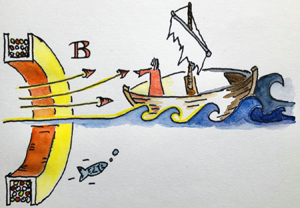
And the same day, when the even was come, he saith unto them, Let us pass over unto the other side. 4:36 And when they had sent away the multitude, they took him even as he was in the ship. And there were also with him other little ships. 4:37 And there arose a great storm of wind, and the waves beat into the ship, so that it was now full. 4:38 And he was in the hinder part of the ship, asleep on a pillow: and they awake him, and say unto him, Master, carest thou not that we perish? 4:39 And he arose, and rebuked the wind, and said unto the sea, Peace, be still. And the wind ceased, and there was a great calm (Mark 4:35–39, KJV Emerald Text Bible 2006).
Indeed, since the beginning of navigation, men have been threatened by waves, generated by wind blowing over the surface of water. The velocity difference across the interface between the air and the water drives the waves, as was demonstrated in early experiments by von Helmholtz (Reference von Helmholtz1868) and his friend Lord Kelvin (Thomson Reference Thomson1871). Their seminal works have given rise to the term Kelvin–Helmholtz instability (KHI) for this phenomenon.
Besides being a hazard, water waves are also an economic nuisance. According to Scheidt (Reference Scheidt2012), sea disturbances increase the fuel consumption of ships on all oceans by 3 %. Apart from divine intervention, oil poured onto the sea calms the waves, as reported already by Aristotle, Plutarch and Pliny the Elder (Scott Reference Scott1978). Landerer (Reference Landerer1894) even conducted test experiments to discover which type of oil has the best effect. However, this method has become obsolete because of pollution control. In contrast, the calming effect of rain on sea disturbances (Tsimplis Reference Tsimplis1991) is harmless, but does not happen on schedule. However, externally applied electric and magnetic fields can be switched on at will. But due to the tiny magnetic susceptibility of diamagnetic water ( $\chi \approx - 10^{-5}$) the latter have no effect for sea disturbances.
The same is not true for ferrofluid, a colloidal dispersion of magnetic nanoparticles (Rosensweig Reference Rosensweig1985), which has a huge susceptibility in the range of  $0 <\chi < 10$. It has been established both theoretically (Gailitis Reference Gailitis1977; Friedrichs & Engel Reference Friedrichs and Engel2001) and experimentally (Cowley & Rosensweig Reference Cowley and Rosensweig1967; Gollwitzer et al. Reference Gollwitzer, Matthis, Richter, Rehberg and Tobiska2007; Richter & Lange Reference Richter, Lange and Odenbach2009) that a magnetic field oriented normally to the static liquid layer destabilizes the interface. In contrast, early experiments for the tilted field instability in a resting layer of ferrofluid (Barkov & Bashtovoi Reference Barkov and Bashtovoi1977; Bercegol et al. Reference Bercegol, Charpentier, Courty and Wesfreid1987) have shown that a horizontal field component can stabilize the interface. This has been quantitatively confirmed by theory (Friedrichs Reference Friedrichs2002) and experiments (Reimann et al. Reference Reimann, Richter, Knieling, Friedrichs and Rehberg2005; Groh et al. Reference Groh, Richter, Rehberg and Busse2007).
Also for the KHI, the stabilizing effect of a tangential magnetic field, or more precisely the shift of the onset of the linear instability to higher flow velocities, was predicted in a seminal theoretical work by Sutyrin & Taktarov (Reference Sutyrin and Taktarov1975). Later it was modelled by Rosensweig (Reference Rosensweig1985), Malik & Singh (Reference Malik and Singh1992), Elhefnawy (Reference Elhefnawy1995) and Zakaria (Reference Zakaria2003). Whereas most models consider two layers of inviscid liquids in two dimensions, and are taking advantage of a velocity potential, more realistic calculations, such as those by Elhefnawy & Moatimid (Reference Elhefnawy and Moatimid2001), are few and far between. Taking into account viscosity, a three-dimensional confinement and a nonlinear magnetization curve, Yecko (Reference Yecko2009, Reference Yecko2010) simulated a low Reynolds number channel flow and concluded that the ‘stabilizing effect’ of a tangential magnetic field may be an oversimplification. This calls for an experiment.
For fluid under motion, the stabilizing effect of a horizontal magnetic field has so far been measured only by Zelazo & Melcher (Reference Zelazo and Melcher1969) for ferrofluid sloshing in a tank. To the best of our knowledge, the magnetic stabilization of the KHI for a magnetic liquid interface has never been explored experimentally in a macroscopic channel. This deficiency is somewhat surprising, because in plasma physics the stabilizing effect of magnetic fields on the KHI was examined in both theory (D'Angelo Reference D'Angelo1965) and experiment (D'Angelo & Goeler Reference D'Angelo and Goeler1966) long ago. Especially in the plasma of the solar corona, magnetic stabilization has been observed to play an important role (Foullon et al. Reference Foullon, Verwichte, Nakariakov, Nykyri and Farrugia2011). Recently Li et al. (Reference Li, Zhang, Yang, Hou and Erdélyi2018) showed evidence of the KHI emerging in between solar blowout jets guided by magnetic flux tubes. This is happening in such a way that the magnetic field is inherently tangential to the interface between the flux tubes.
In this article we report on earthbound experiments for a magnetic liquid interface in order to fill the above-mentioned gap. The article is organized as follows. As an introduction for the reader we present in § 2 the governing equations. Next, in § 3, the experimental set-up and the ferrofluid are characterized. Besides exploring spontaneously emerging interface waves we want to investigate as well waves of well defined frequency (and wavenumber). Therefore we sketch in the same section two different methods of periodic wave excitation. Our experimental results are reported in § 4. From the measured growth and decay rates of the interface undulations we determine the critical flow velocity for various excitation frequencies and applied magnetic fields. In addition we use the driving to measure the dispersion relation of the interface waves. The article finishes with a summary, discussion, and outlook (§ 5).
2. Governing equations
To deduce the dispersion relation for interfacial waves one may assume a two-dimensional system as shown in figure 1. It consists of two superposed layers of inviscid immiscible fluids of different densities  $\rho _a < \rho _b$. In agreement with the experiments the magnetic fluid with magnetic susceptibility $\chi$ is at rest in the top layer, whereas the diamagnetic fluid below is moving with constant velocity $U$. Note that this upside-down version of the classical arrangement (‘wind blowing over the sea’) is motivated by the availability of immiscible diamagnetic and superparamagnetic fluids (cf. § 3). For a flat interface the heights of the upper and lower layer are described by $a$ and $b$, respectively. The interfacial tension $\gamma$ between the two fluids is stabilizing the interface. Because we neglect viscosity and consequently shear stresses, we can assume a non-continuous velocity profile. We apply a homogeneous magnetic field of magnitude $H$ parallel to the unperturbed interface. In a linear stability analysis all small disturbances from the basic state are analysed into normal modes, i.e. they are described by the function $A(x,t)$ in the coordinate system given in figure 1. A linear wave, propagating in direction of the flow, is described by
 \begin{equation} A(x,t) = A_0\,\textrm{Re}\{ \textrm{e}^{\textrm{i}(kx-\omega t)}\}, \end{equation}
where the wavenumber  $k$ or the frequency $\omega$ can be complex, and one obtains a linear instability in space or time, respectively. An additional phase is not necessary for our purposes and can be omitted. For $\textrm {Im}(\omega )>0$, surface undulations will grow exponentially and the flat interface is unstable. Following the standard procedure of linear stability analysis, the dispersion relation of linear interface waves for semi-infinite layers can be derived (Sutyrin & Taktarov Reference Sutyrin and Taktarov1975; Rosensweig Reference Rosensweig1985), which reads in our notation
 \begin{equation} \omega^2 \rho_a + (\omega - kU)^2\rho_b = kg(\rho_b-\rho_a) + k^3\gamma + k^2 \tilde{\mu} H^2. \end{equation}
Here  $g$ denotes the gravitational acceleration, and $\tilde {\mu } = \mu _0 \chi ^2/(\chi +2)$ is proportional to the vacuum permeability $\mu _0$ and depends on the susceptibility $\chi$. Note that we can neglect here the effect of the finite layer thicknesses $a$ and $b$, because the observed wavenumbers are sufficiently high. The dispersion relation (2.2) can be written in the form
 \begin{equation} \omega_{1,2} = \underbrace{kU\frac{\rho_b}{\rho_a+\rho_b} }_{\hat{\omega}} \pm \underbrace{ \sqrt{ \frac{k^3\gamma}{\rho_a+\rho_b} - \frac{k^2U^2\rho_a \rho_b}{(\rho_a+\rho_b)^2} + \frac{k^2 \tilde{\mu} H^2}{\rho_a+\rho_b} + kg\frac{\rho_b-\rho_a}{\rho_a+\rho_b}}}_{\tilde{\omega}}, \end{equation}
giving a convenient equation for the instability in time. The right-hand side of (2.3) is made up of two terms. The first one,  $\hat {\omega }$, describes a convective movement with the constant velocity $\omega /k$ proportional to the flow velocity $U$. It vanishes for $U=0$ (see figure 2a), whereas it increases linearly with $k$ for $U>0$, as marked in figure 2(b–d) by a dashed black line. The second term, $\tilde {\omega }$, has a positive (negative) root, which is plotted in figure 2 by a green (blue) solid line, respectively. Under the root are three positive addends and one negative one. Both the second and the third addend depend on $k^2$. Obviously an increase in terms $U^2$ can be compensated by an increment in terms $H^2$. As long as $\tilde {\omega }$ is real, the amplitude of the wave remains the same. For a negative discriminant, however, $\tilde {\omega }$ becomes imaginary, which leads to a stable and an unstable branch in the dispersion relation. This destabilization occurs for a certain range of wavenumbers if the flow velocity $U$ is sufficiently high. On the other hand we can stabilize the system by increasing the surface tension, the density difference or, in our case, the applied magnetic field.

Figure 1. Illustrative sketch of the flow configuration.

Figure 2. Dispersion relation  $\omega (k)$ of interfacial waves illustrated for $H=0$ kA m $^{-1}$ and four different flow velocities $U$:
$U$:  $U=0$ (a), $U \lesssim U_{\mathit {crit}}^0$ (b), $U=U_{\mathit {crit}}^0$ (c) and $U \gtrsim U_{\mathit {crit}}^0$ (d). The different colours show the two branches for $\omega _1$ and $\omega _2$. Solid lines represent the real part, dotted lines the imaginary part of $\omega$. The dashed line represents the convective term $\hat {\omega }$.
Figure 2 shows the transition from a stable to a linearly unstable interface without an applied magnetic field. If  $U=0$ m s $^{-1}$, as displayed in figure 2(a), the dispersion relation is the same as for ordinary interface waves with a capillary and a gravitational term. The green (blue) branch is associated with waves moving in the positive (negative) direction, respectively. When we increase the flow velocity $U$ the two branches move closer together (cf. panel b) and for the critical velocity $U_{\mathit {crit}}^0$ the branches touch each other at the critical wavenumber $k_{\mathit {crit}}^0$, as shown in panel (c). For higher velocities $U > U_{\mathit {crit}}^0$ there is a band of unstable wavenumbers between $k_2$ and $k_3$ (panel d).
Of special interest is not only the velocity of the first occurrence of unstable waves  $U_{\mathit {crit}}^0$, but also the critical velocity $U_{\mathit {crit}}$ for an arbitrary wavenumber $k$ or wave frequency $f = \omega /2\pi$, corresponding to the neutral curve. The critical velocity depending on the wavenumber can be calculated by solving the equation $\tilde {\omega } = 0$ s $^{-1}$ for the velocity $U$. It is given by
 \begin{equation} U_{\mathit{crit}}(k,H) = \sqrt{\frac{\rho_a+\rho_b}{\rho_a \rho_b}\left(k\gamma + \tilde{\mu}H^2+\frac{g\left(\rho_b-\rho_a\right)}{k}\right)} \end{equation}
and is depicted in figure 3(a).
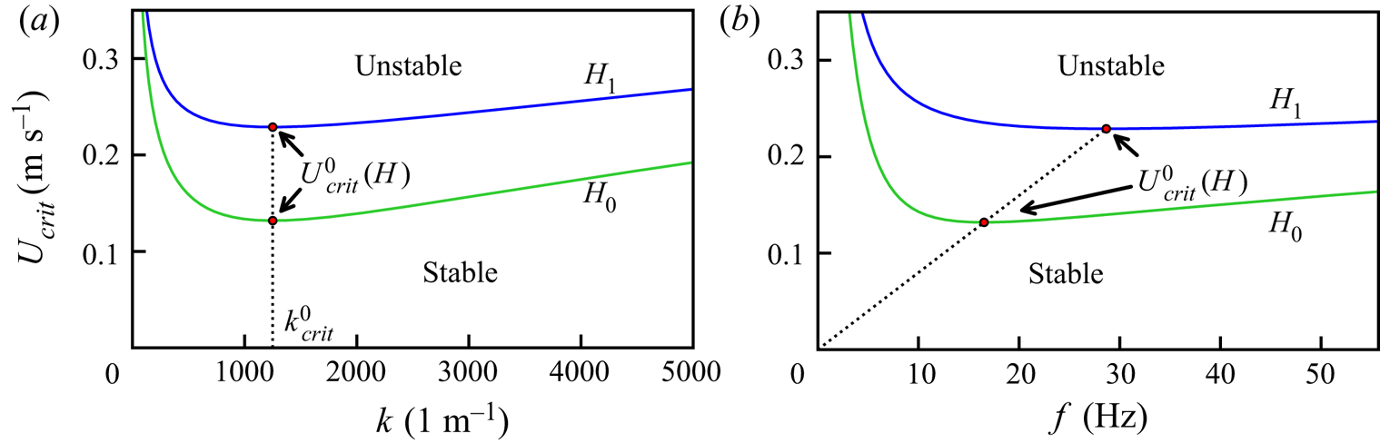
Figure 3. Stability maps for different magnetic fields  $H_0=0$ kA m $^{-1}$ (green line) and $H_1=10$ kA m $^{-1}$ (blue line). For system parameters please see § 3. The solid lines show the dependency of the critical velocity $U_{\mathit {crit}}$ on the wavenumber $k$ (a) and the frequency $f$ (b). The dots mark the wavenumbers and frequencies of the first occurrence of the instability. The dotted lines connect these points.
So far we have examined the instability in time. However, in our experiment it is advected by the flow and examined in space. For the related stability map, showing the critical velocity as a function of  $f$, an analytical expression cannot be found easily, as a cubic equation must be examined. The numerical solution, however, is shown in figure 3(b). As one can see in figure 3 and (2.4) a magnetic field $H>0$ stabilizes the system and shifts the neutral curves to higher flow velocities for all wavenumbers and frequencies (cf. blue lines). Its minimum, the velocity of the first unstable waves $U_{\mathit {crit}}^0$, occurs at the capillary wavenumber $k_{\mathit {crit}}^0 = \sqrt {g(\rho _a+\rho _b)/\gamma }$ (Cowley & Rosensweig Reference Cowley and Rosensweig1967), and is independent of the wavenumber $k$, as marked in figure 3(a) by the dotted vertical line. In contrast, as illustrated in figure 3(b), the frequency of the minimum depends linearly on the velocity $U_{\mathit {crit}}^0$ via the convective term $\hat {\omega }$ in (2.3) where $\tilde {\omega }=0$.
3. Experiments
First we give an overview of the experimental apparatus (§ 3.1), and then we present the material parameters of the two fluids used in the experiment (§ 3.2). Thereafter, the method used to measure the flow velocity is described (§ 3.3). In § 3.4, we give details on how the liquid interface is determined from the recorded pictures. Eventually we sketch the magnetic (§ 3.5) and mechanical (§ 3.6) devices utilized for the local excitation of waves of preset frequency.
3.1. Experimental set-up
The heart of our experimental set-up is sketched in figure 4(a). A straight section of the flow channel, made from Perspex©, harbours the liquid interface in between the ferrofluid on top and a more dense, immiscible and transparent fluid on the bottom. This interface section of the channel has a length of 150 mm ( $x$-direction), a width of 25 mm ( $y$-direction) and a height of 45 mm ( $z$-direction). Here the flow channel is vertically divided into two sections. The upper one contains 100 ml of ferrofluid, marked black in figure 4(a), and has a height of 20 mm. It has a wedged shape of inclination 45 $^\circ$ to the horizontal. This sharp edge at the upstream side (left-hand side) serves to foster the shear flow. The ramp at the downstream side (right-hand side), with an inclination of 17 $^\circ$, serves to suppress the standing waves in the channel. Note that the inclined edges also reduce the discontinuity of the magnetization at the up- and downstream sides of the channel. This is similar to the ‘radial ramp’ introduced by Gollwitzer et al. (Reference Gollwitzer, Matthis, Richter, Rehberg and Tobiska2007) for measuring the Rosensweig instability in a circular vessel. Moreover, by matching the dimensions of the channel and the Helmholtz pair of coils we have created a ‘magnetic beach’. In this way the magnetic field fades out at both ends of the interfacial section. The resulting Kelvin force density $\mu _0 (\boldsymbol {M} \boldsymbol {\cdot } \boldsymbol {\nabla })\boldsymbol {H_0}$ (Rosensweig Reference Rosensweig1985) plus the ramps are sufficient to contain the ferrofluid within the interfacial section of the channel. There are two openings at the top of the channel. The first one, at the upstream side, is used for filling the upper section with ferrofluid, whereas the second one allows the insertion of a magnetic (§ 3.5) or mechanical (§ 3.6) exciter, or a plug. The lower part of the flow channel has a height of 25 mm and a width of 25 mm, and it guides a laminar flow of transparent fluid.

Figure 4. Sketch of the flow channel. In its interfacial section the ferrofluid rests on top of a flow of transparent fluid (a). The interfacial section is part of a stadium-shaped conduit (b) and is placed in the centre of a Helmholtz pair of coils. The magnetic field generated by these coils is matched to the ferrofluidic section of the channel (c). The data points denote measurements of the axial magnetic field, while the solid line denotes the calculated values for the applied current of 3.0 A for a Helmholtz pair of coils according to (3.1). The vertical dashed line connecting panels (a) and (c) marks the position of the exciter, the origin of our coordinate system. A photo of the set-up can be found elsewhere (Völkel, Kögel & Richter Reference Völkel, Kögel and Richter2020).
The interface is illuminated from the back by means of an electroluminescent sheet (Zigan displays). To prevent the ferrofluid from wetting the side walls of the channel we attach strongly repellent Teflon© tape (3M $^{\mathrm {TM}}$ PTFE Extruded Film Tape 5490) to them. Because the thickness of the tape is $0.09$ mm it will hardly accelerate the flow within the channel.
As shown in figure 4(b), the interface section of the flow channel, described above, is part of a larger stadium-shaped duct, which is made up of two semi-circles ( $d_{\mathit {inner}}= 290$ mm, $d_{\mathit {outer}}=340$ mm) and two straight sections ( $\textrm {length}=340$ mm), and which harbors 1200 ml of transparent fluid. The latter is put in motion by a propeller with a diameter of 20 mm (cf. right-hand side of figure 4b). The flow is relaminarized by a honeycomb structure embedded in the straight section following the propeller. The propeller is driven by an electric motor (Mattke MDR 230/2-4). The latter is controlled via an RS.232 interface by a computer. To minimize electromagnetic disturbances the propeller and the motor are connected via a 340 mm long shaft. Note that a similar channel has worked well for Barchan dunes (Groh, Rehberg & Kruelle Reference Groh, Rehberg and Kruelle2009). The experimental channel is positioned in the centre of a Helmholtz pair of coils, which allows us to apply a magnetic field oriented parallel to the flow direction of the lower fluid and so parallel to the interface. The coils have a usable clearance of 240 mm (diameter) and 88 mm (distance). Their effective radius is $R=90$ mm. We measure the magnetic induction $B$ in the empty coils by means of a Hall probe (Lakeshore, MMT-6J02-VH). The applied magnetic field $H=B/\mu _0$ obtained in this way is plotted in figure 4(c) by black points. The solid line displays a fit by the equation (Bergmann & Schaefer Reference Bergmann and Schaefer2006)
 \begin{equation} H(x) = \frac{NI}{2R}\left\{ \left[\left(\frac{x-x_0}{R}-\frac{1}{2}\right)^2+1\right]^{-3/2} + \left[\left(\frac{x-x_0}{R}+\frac{1}{2}\right)^2+1\right]^{-3/2} \right\}, \end{equation}
where  $x_0=5.7$ cm denotes the centre of the Helmholtz pair of coils, $N=640$ is the number of windings and $I$ is the current. From the measurements we conclude that $H$ does not deviate more than 0.5 % along the visible part of the channel (Kögel Reference Kögel2017). The coils are connected to a direct current source (LAB/SL 230/AI/LT from Eurotest Co.) which is controlled via GPIB interface by the computer.
Pictures of the liquid interface are recorded by a charge-coupled-device (CCD) camera (Lucam Lt225M, Lumenera Co.) which is triggered by a multichannel function generator (TGA1244, TTi Co.) with a frequency of 100 Hz.
3.2. Properties of the fluids
For the upper fluid we select the ferrofluid Electro Magnetic Grade (EMG) 909 from Ferrotec Co. Its material parameters are listed in table 1. The magnetization curve  $M(H)$ of the ferrofluid has been recorded by means of a vibrating sample magnetometer (VSM), namely Lakeshore 7404 from Cryotech, utilizing a spherical sample holder (Friedrich et al. Reference Friedrich, Lang, Rehberg and Richter2012). The $M(H)$ curve and its granulometric characterization by means of a superposition of Langevin functions has been presented by Rehberg, Richter & Hartung (Reference Rehberg, Richter and Hartung2019), yielding the listed initial susceptibility $\chi _0$. The diamagnetic fluid below is the perfluoroether Galden SV90 from Solvay Solexis, as utilized before (Sterr et al. Reference Sterr, Krauß, Morozov, Rehberg, Engel and Richter2008; Poehlmann, Richter & Rehberg Reference Poehlmann, Richter and Rehberg2013). Its susceptibility has been measured by the VSM as well, and is included in table 1 for the sake of completeness. Because of its tiny value it can be neglected. The interfacial tension between the two fluids has been measured by means of a drop volume tensiometer (Lauda TVT2). The densities of both fluids have been determined by an electronic density meter (DMA 4100, Anton Paar Co.). The viscosities of both fluids were measured with the rheometer MCR 500 (Anton Paar Co.) utilizing the double gap geometry (type DG 26,7).
Table 1. Properties of the fluids EMG 909 (Lot No. H030308A) from Ferrotec Co. and Galden SV90 from Solvay (2017) Solexis.

3.3. Velocity measurement
We measure the velocity profile of the moving fluid with an ultrasonic Doppler velocimeter (DOP 3000 from Signal Processing). We use polyamide particles (Griltex 2A P1) for scattering particles with diameters from 50 to 80  $\mathrm {\mu }$m and a density of 1005 kg m $^{-3}$. As the density of the particles is less than the density of the transparent fluid, we measured the speed at which the particles ascend in the fluid. This speed is $(3\pm 2)$ mm s $^{-1}$ and therefore much less than the flow velocity during the experiments, which is typically above 100 mm s $^{-1}$. Hence we can assume the particles essentially follow the streamlines of the moving fluid. A velocity profile, averaged over six measurements, is shown in figure 5. The large error bars for $y\gtrapprox 18$ mm are caused by a non-perfect coupling of the ultrasonic probe to the lid of the channel. Likewise, the measurements are distorted by scattering on different interfaces and the surface of the ultrasonic gel used. As we expect a symmetric velocity profile, the measurements at $y<18$ mm are sufficient for determining the whole profile. The maximal flow velocity $U$ in the channel was found (Kögel Reference Kögel2017) to depend on the rotation frequency $\nu$ of the motor according to
 \[ U(\nu) = (9.5 \times 10^{-5}\ \nu\ \mathrm{r.p.m.}^{-1} - 4.5 \times 10^{-2})\ \mathrm{m\,s}^{-1}. \]
Figure 5. Averaged velocity profile  $v(y)$ after six measurements at a motor speed of 2000 rpm. The dashed lines indicate the lid ( $y=25$ mm) and the bottom ( $y=0$ mm) of the channel. The red solid line shows a parabolic fit, as a convenient approximation.
3.4. Detection of the interface
In figure 6(a) we present a typical photo of the liquid interface between the ferrofluid (above) and the transparent fluid (below). In panel (b) we plot the brightness along the vertical line, marked green in (a). Each line can be fitted by the error function marked by the red solid line in (b). The point of symmetry of the former defines the position of the interface. Panel (c) indicates the detected interface by a yellow solid line.

Figure 6. Typical photo of the interface (a) and greyscale along one vertical line (b), which is marked green in panel (a). The red solid line denotes a fit by the function  $h(y) = A\, \textrm {erf}(B(y-y_0)) + h_0$, where $\textrm {erf}$ denotes the error function. The detected typical interface is marked in yellow in panel (c). For display purposes the detected interface was rounded to full pixels.
3.5. Magnetic excitation
In order to excite a surface wave with a defined frequency  $f$, either a local electric excitation (Leiderer, Ebner & Shinkin Reference Leiderer, Ebner and Shinkin1982), a local blowing (Mahr, Groisman & Rehberg Reference Mahr, Groisman and Rehberg1996), or a local magnetic excitation (Browaeys et al. Reference Browaeys, Bacri, Flament, Neveu and Perzynski1999) has been used for measuring the dispersion relation of a quiescent liquid layer. In our case the challenge was to apply a magnetic induction $B_{\bot }$, oriented normal to the interface, at and only at a position $x_0$ of the interface; i.e. $B_{\bot }(x) \approx B_{\bot }^0 \cdot \delta (x-x_0)$. At the same time the induction $B_{\bot }$ should not vary across the channel; i.e. $B_{\bot }(y)=\textrm {const}$. For that purpose an iron sheet (thickness of 2 mm, length of the stem 55 mm, height of the blade 12 mm) was wrapped by a wire ( $\varnothing$ 1.0 mm, 70 windings), as shown in figure 7(a). The iron sheet has a grater-like shape, with a triangular cutting edge at its lower end (b). In this way it guides the magnetic flux towards a position 2 mm above the interface. The corners of the blade next to the channel walls are slightly rounded in order to suppress fringe fields there (b). As shown in figure 8(a), the magnetic induction, measured by means of a Hall probe immediately beneath the blade, is still higher at the corners, but does not vary more than 25 % across the width of the channel. Likewise, figure 8(b) presents both components of the induction, measured in the centre of the channel for increasing distance from the exciter. The solid lines indicate fits by an exponential decay, and thus illustrate that the type of excitation is sufficiently local.The magnetic driving is based on the Kelvin force density $f_{\mathit {K}}=M_{\mathit {FF}}(H) \cdot \partial B/ \partial z$ which is acting upon the ferrofluid with magnetization $M_{\mathit {FF}}(H)$. We vary $f_{K}$ by a periodic modulation of $\partial B/ \partial z$ by modulating the magnetization $M_{\mathit {st}}(t)$ of the steel sheet. This is achieved by driving the coils by a current source (LAB/SL 30 from Eurotest Co.), connecting its voltage contol input to the voltage output of a function generator (TGA1244 from TTi Co.) connected to the computer. For all experiments we selected $U_{\mathit {DC}}=2.5$ V and $U_{\mathit {AC}}=5.0$ V, where $U=U_{\mathit {DC}} + U_{\mathit {AC}} \sin {(2 \pi f t)}$ gives the overall applied control voltage.
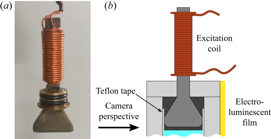
Figure 7. Magnetic driving of the interface by means of a local coil with soft iron core (a), mounted 2 mm above the interface (b).

Figure 8. Spatial variation of the magnetic induction: (a) Vertical component measured directly beneath the blade of the magnetic exciter, where the dashed vertical lines indicate the walls of the channel. (b) Horizontal and vertical component of the exciter measured in a distance  $x$ down the stream. Here the solid lines mark fits by an exponential decay: $B_\parallel (x) \approx 5.5\ \mathrm {mT} \cdot \exp (-x/11.0\ \mathrm {mm})$, $B_\perp (x) \approx 4.6\ \mathrm {mT} \cdot \exp (-x/4.7\ \mathrm {mm})$. For the measurements a Hall probe (type MNA-1904-VH, from Lakeshore Co.) connected to a Gaussmeter (type 450, from Lakeshore Co.) was used.
Figure 9(a) displays the discrete Fourier transform (DFT) of the temporal evolution of the interface at distances of  $x=20$ mm (blue), 30 mm (red) and 40 mm (green) downstream of the magnetic exciter. The dominating peaks at 8 Hz prove the efficiency of the driving. The inset provides a zoom of the peaks, which decay with increasing distance $x$. Likewise, the time-averaged autocorrelation function in figure 9(b) shows a decay as well. From its first relative maximum, marked by a red dot, the wavelength $\lambda$ can be determined.

Figure 9. Dynamics of the interface for a driving frequency of  $f_0= 8$ Hz, a flow velocity $U=0.126$ m s $^{-1}$ and a magnetic field $H=8.0$ kA m $^{-1}$: (a) Digital Fourier transform $\tilde {y}$ of the wave amplitude for three sample $x$-positions. The inset gives a zoom around the peaks at 8 Hz. (b) Averaged autocorrelation function $Y$ vs space. The estimated data are marked by dots, the solid line indicates a fit by a cubic spline, and the red dot denotes the first local maximum.
From the results above as well as from our experience, it follows that the magnetic exciter allows a reliable and smooth driving of the interface. However, an unwanted side effect is the fact that the soft iron core will be magnetized not only by the driving current, but also by the horizontal induction impressed by the static field applied by the Helmholtz pair of coils. We therefore investigated as a reference method a mechanical excitation, which is presented next.
3.6. Mechanical excitation
The mechanical exciter is sketched in figure 10(a). The interface is perturbed by a horizontal bar (see blow-up in panel b) connected via a vertical shaft to an electro-mechanical vibration exciter (Brüel & Kjær, type 4810, with amplifier type 2706). The bar has a length of  $24.7\pm 0.1$ mm, thus filling almost the whole width of the channel. A lead-through with adjustable O-ring allows a leak-tight reciprocating motion of the shaft. Bar, shaft and lead-through are made from brass, a material with negligible susceptibility. The shaft is attached to a $U$-shaped module (made from aluminium), which transfers the motion, bypassing one of the coils.

Figure 10. Set-up of the mechanical wave exciter, with a horizontal bar at the interface, attached to a vertical shaft (a), and detail of the lead-through with O-ring sealing (b). Panel (b) is rotated against panel (a) by  $90^\circ$.
We have measured the magnetic stray field of the exciter by means of a Hall probe (type MNT-4E02-VG, from Lakeshore Co.), as marked in figure 11 by red circles. The solid line displays the characteristic decay of  $B(z)$ on the axis of a dipole. Already at a distance of 200 mm the stray field is below the bias (marked by squares) determined by the earth's magnetic field. Thus we have positioned the shaker 220 mm above the flow channel. For a reliable, stick-free driving it is important to fine-tune the position of the shaker in the plane by a micrometre stage for the x- and by one for the y-direction.

Figure 11. Decay of the constant stray field vs distance measured by means of a Hall probe (filled red circles). The red solid line represents a fit by  $B_z(z)=\mu _0 m /(2 \pi z^3)$, with $m=(1.23 \pm 0.03)\ \text {Am}^2$. The open black squares give the data of the magnetic background.
The mechanical driving might be expected to outperform the magnetic one, because it does not perturb the applied magnetic field. However, it turned out to depend sensitively on the position of the meniscus at the driving bar, as illustrated in figure 12. In panel (a) the interface is pinned by the lower edge of the bar, as indicated by the red arrow, whereas in panel (b) the interface is not pinned. In panel (c) we plot the driving amplitude vs the distance from the exciter, measured for two sample flow velocities. The driving amplitude shows only a weak dependence on the flow velocity for the pinned menisci (solid lines) but a strong dependence for the unpinned menisci (dashed lines). Therefore, prior to measurements, the meniscus was carefully pinned at the lower edge. More details are given by Fischer (Reference Fischer2017). As in § 3.5 we show in figure 13 the DFT of the temporal evolution of the interface for three chosen driving frequencies. The amplitude at the excitation frequency (indicated by arrows) is clearly dominating the spectra.

Figure 12. Effect of the pinning of the meniscus on the driving: pinned (a) and loose (b) menisci, as indicated by red arrows, at the horizontal bar of the exciter, and related amplitudes  $A$ vs distance $x$ from the exciter measured for two different flow velocities $U$, as denoted by the inset (c).

Figure 13. Frequency spectrum of the interface at a distance of 10 mm downstream of the mechanical exciter, for an excitation with  $f_0=3$ Hz (blue), 10 Hz (red) and 20 Hz (green). The excitation frequency is annotated by arrows. The flow velocity was 0.145 m s $^{-1}$.
4. Experimental results
In the following we give experimental evidence of a calming of the waves by a magnetic field (§ 4.1) and present exemplary measurements of the growth rates of the interface undulations (§ 4.2), the stability diagrams derived therefrom (§ 4.3), and eventually the measured dispersion relation (§ 4.4).
4.1. Experimental evidence
The application of a tangential magnetic field has immediate impact on the amplitude of the interfacial waves. Figure 14(a) shows a snapshot of spontaneous waves. When an induction of  $B=10$ mT is applied, the amplitudes are considerably damped, as presented in figure 14(b). From the snapshot in figure 14(a) it becomes clear that the spontaneously generated waves show a broad spectrum of wavelengths. For a sensible comparison with the model of § 2 it is advantageous to excite waves of a preset frequency $f$ (and wavelength) by magnetic or mechanical means, as shown in figures 14(c) and 14(e), respectively. Likewise figures 14(d) and 14(f) demonstrate the calming effect of a horizontal magnetic field at the same parameters. Next we exploit this arrangement for measuring the growth rates of the interfacial waves.

Figure 14. Experimental evidence for a calming of the interfacial waves at  $U=0.192$ m s $^{-1}$. Spontaneously emerging waves without an externally applied magnetic induction (a), and for $B=10$ mT (b). Magnetically generated waves without (c) and with (d) applied induction $B=10$ mT. Mechanically generated waves without (e) and with (f) applied induction $B=10$ mT. A movie demonstrating this effect when switching on $B$ can be accessed at https://doi.org/10.1017/jfm.2020.642. The frames have a size of $117~\textrm {mm} \times 10~\textrm {mm}$.
4.2. Growth rates
First we utilize the magnetic exciter (see § 3.5), which defines the position  $x=0$ mm in our frame of reference, and apply a driving with frequency $f \in$ [6 Hz, 20 Hz]. For each position $x$ along the interface we determine the amplitude $A(x)$ of surface undulations by means of a DFT. As an example we illustrate the outcome of this procedure in figure 15(a) for $f=11$ Hz and four sample flow velocities $U$. For the subcritical flow velocities ( $\cdot$, $\circ$) the amplitude decays, whereas for supercritical values ( $\Box$, $\diamond$) it grows downstream of the exciter. In the interval [0 mm, 20 mm] the amplitude $A(x)$ appears to follow an exponential law
 \begin{equation} A = A_0\exp(\alpha x), \end{equation}
where  $\alpha$ denotes the growth or decay rate along $x$. The corresponding fits are marked in figure 15(a) by solid lines. Further from the exciter the growth of $A(x)$ does not follow the linear stability analysis (4.1), possibly due to the viscosity and the friction at the side walls, which is not taken into account in the simple ansatz.

Figure 15. Growth of surface waves: (a) amplitude vs the distance from the exciter along the direction of the flow at a driving frequency of  $f=11$ Hz without horizontal magnetic induction, i.e. $B_x =0$ mT. The inset indicates the symbols marking four different flow velocities. The straight lines denote an exponential fit by (4.1). (b) The data points indicate the measured growth rates vs the flow velocity for different values of the horizontally applied magnetic induction. To guide the eyes the data points are interpolated by cubic splines (solid lines).
The growth rates  $\alpha$ determined from these fits depend sensitively on $U$, but also on the horizontally applied magnetic field $H$, as shown in figure 15(b). For a fixed field $H$ the growth rate $\alpha$ increases with $U$, becoming unstable at $\alpha (U_{\mathit {crit}}) = 0$. Increasing the field $H$ shifts the $\alpha (U)$ curves to the right, thereby shifting $U_{\mathit {crit}}$ to higher velocities. In this way the interface remains stable up to a higher velocity.
In order to check the reliability of the magnetic driving we have performed similar experiments utilizing the mechanical exciter described in § 3.6. Figure 16 compares the two methods of excitation for two representative values of the applied magnetic field. Data points obtained with the mechanical bar are denoted by squares ( $\Box$), and those with the magnetized wedge by a triangle ( $\triangledown$). To guide the eyes the data are interpolated by splines. For both types of excitation the critical growth rate $U_{\mathit {crit}}$ is shifted with $H$ to higher values by about the same amount (dashed, $\Delta U_{\mathit {crit.mech}}=0.017$ m s $^{-1}$; solid, $U_{\mathit {crit.mag}}=0.018$ m s $^{-1}$). Indeed, the differences for $\Delta U_{\mathit {crit}}$ are well situated in the range of the error bars. Because the magnetic driving is more robust – it does not sensitively depend on the proper pinning of the meniscus – we present in the remainder of the article solely the data obtained by magnetic excitation.

Figure 16. Comparison of the growth rates for waves generated with a modulated magnetized iron wedge ( $\triangledown$) and mechanical driving with a bar with square cross-section ( $\Box$) for different horizontally applied fields $H$ and various flow velocities at $f=10$ Hz. The amplitude of the mechanical exciter was 0.14 mm. To guide the eyes the data are interpolated by splines (omitting the outlier at $U=0.166$ m s $^{-1}$ for $H=2.0$ kA m $^{-1}$).
4.3. Stability diagrams
4.3.1. Periodically excited waves
We have determined  $U_{\mathit {crit}}$ for different driving frequencies and applied magnetic fields. Three exemplary sets of data are shown in figure 17(a) together with solid lines calculated via (2.4) for the material parameters of table 1. The data points for zero magnetic field ( $\cdot$) are well described by the basic inviscid model. This is especially true for the interval [10 Hz, 20 Hz]. At lower $f$ the increase of the experimental values is delayed when compared with the inviscid model. At a magnetic field of $H=4.0$ kA m $^{-1}$ the experiment ( $\circ$) and the inviscid model are in closer agreement in the same interval, i.e. [5 Hz, 10 Hz]. Here, however, the experimental data exceed the model predictions in between 14 and 20 Hz. For $H=8.0$ kA m $^{-1}$ ( $\Box$) the agreement seems to become better again. However, here the error bars are quite large, because $U_{\mathit {crit}}$ needs to be estimated by extrapolation. Comparing the three curves in figure 17(a) it is obvious that with increasing magnetic field the stability curves are shifted to higher values. This reflects the calming of the waves. Indeed, as shown in figure 17(b) for an exemplary driving frequency of $f=10$ Hz, the measured critical velocity follows very well the predicted curve (blue solid line). At lower $H$ (red line) the agreement is less convincing.

Figure 17. (a) Critical flow velocity vs driving frequency for three exemplary magnetic fields. The dashed vertical lines indicate the frequency scans for  $f=6.0$ and 10.0 Hz displayed in panel (b). The solid lines represent the inviscid model (2.4).
All in all the basic inviscid model, which has no free parameter, captures the measured stability diagrams rather well. Deviations may stem from the difficulty of defining an effective jump of the flow velocity in the experiment. For an in-depth discussion the reader is referred to § 5.
4.3.2. Spontaneously emerging surface waves
So far we have investigated the stability of surface waves generated by a periodic driving. Two exemplary curves without (with) a magnetic field are marked in figure 18 by black data points. The solid lines indicate the predictions by the basic inviscid model. With respect to these stability diagrams it is interesting to see that the spontaneously generated surface waves, denoted by red diamonds, are situated slightly above, but apparently fit rather well to the theoretical stability curve (black solid line). However, we point out that the agreement along the  $x$-axis is less convincing because the spontaneously generated waves are not located at the minimum of the stability curve. The minimum is situated in figure 18(a) at 16.5 Hz and in figure 18(b) at 17.2 Hz. These large differences in $f$ may be attributed to the broad footing of the stability curves.

Figure 18. Comparison of the measured critical velocity for periodically excited waves (black points) and spontaneously emerging waves (red diamonds), without magnetic field (a), and with  $H=2.0$ kA m $^{-1}$ (b). The solid line indicates the prediction by the basic inviscid model.
These spontaneous surface waves emerge because the flow generated by the propeller is not completely laminar. Despite a relaminarization duct realized by a honeycomb structure in the straight section following the propeller, fluctuations of the interface may emerge. This is in agreement with the Reynolds number ranging from  $\mathit {Re} = 4600$ to $\mathit {Re} = 6300$ for the measurements in figure 18.
4.4. Dispersion relation
In § 2 we have presented in (2.2) the dispersion relation for interfacial waves at the KHI. Our experimental arrangement can also be used to measure this relation. Experimental results are plotted in figure 19 for three representative magnetic fields. We have measured the dispersion relation for nine different velocities  $U\in [0.1,0.207]$ m s $^{-1}$. For brevity and clarity we selected one $U$ with fully stable surface waves (a) and one $U$ exhibiting the transition to unstable surface waves (b). Figure 19(a) shows the measured data for $U=0.126$ m s $^{-1}$ and compares it with the predictions of the simple inviscid model (marked by solid lines). The $f(k)$ curves, numerically obtained from (2.2), increase monotonically, and with increasing $H$ their inclination rises. This is true for the measured data as well as for the numerical results. However, the latter overestimate the measured data considerably. For example, at $k=400\ \textrm {m}^{-1}$ and $H=8.0\ \mathrm {kA\ m}^{-1}$, experiment and model differ by 13 %.

Figure 19. Dispersion relation for  $U=0.126$ m s $^{-1}$ (a) and $U=0.180$ m s $^{-1}$ (b) and three different magnetic fields. The open (filled) data points mark experimental results for stable (unstable) surface waves, respectively. The lines indicate the outcome of the inviscid model (2.2).
The dispersion relation is more complex at a flow velocity of  $U=0.180$ m s $^{-1}$, as displayed in figure 19(b). Whereas for $H=8$ kA m $^{-1}$ all measured data (brown squares) indicate a stable interface, as do the numerics (solid line), one finds for $H=4$ kA m $^{-1}$ (marked green) above $k \approx 300\ \text {m}^{-1}$ the emergence of a convective unstable state, indicated by filled symbols. The numerical solution of (2.2) also predicts a band of unstable wavenumbers, albeit starting at higher $k$, namely at the kink at $k \approx 500\ \text {m}^{-1}$. Likewise, for $H=0$ kA m $^{-1}$, convective unstable waves are measured for $k \gtrsim 300\ \text {m}^{-1}$, whereas the kink predicted by the model is situated at $k \approx 400\ \text {m}^{-1}$. Again all qualitative features of the dispersion relation are met by the basic inviscid model, whereas one finds a quantitative discrepancy in the onset of the unstable band.
5. Summary, discussion and outlook
In a tabletop flow channel we have measured the linear stability of interface waves in between a flow of diamagnetic liquid (on the bottom) and a resting layer of ferrofluid (on the top) – a realization of the Kelvin–Helmholtz instability. We have provided the first experimental evidence that a magnetic field oriented tangential to the liquid surface is capable of calming spontaneously emerging waves. To enable a quantitative comparison with the basic inviscid model reported by Rosensweig (Reference Rosensweig1985), we have periodically perturbed the interface by magnetic or mechanical means. From the zero point of the measured growth rates we have determined the critical flow velocity  $U_{\mathit {crit}}(f,H)$. For $H=0$ and $H=10$ kA m $^{-1}$ the basic inviscid model (2.2) captures $U_{\mathit {crit}}(f,H)$ well, when taking into account that there is no free parameter. It is notable that the characteristic increase in the critical velocity, which is similar to a hyperbolic curve, is also seen in the experiment. Moreover we have presented experimental data of the dispersion relation $f(k,H)$ at two sample flow velocities. Again the basic inviscid model (2.2) predicts an increase of the wavenumber with the driving frequency, in agreement with the experimental findings. Bands of unstable wavenumbers are found both in the model and in the experiments, albeit over different ranges of $k$.
$k$.
In summary, the experiment provides evidence for a calming of interface waves under impact of a tangential magnetic field. Both the critical flow velocity  $U_{\mathit {crit}}(f,H)$ and the dispersion relation $f(k,H)$ display most of the qualitative features predicted by the basic inviscid model.
Quantitative discrepancies may stem from three simplifications:
(i) The measured velocity, as shown in figure 5, is apparently not constant across the channel, a simplifying assumption used in § 2. In contrast, for deriving the governing equations, Rosensweig (Reference Rosensweig1985) assumes a jump in the velocity profile at the interface which is only possible for an inviscid moving fluid. In our experiments, however, the moving fluid has a finite viscosity which leads to a continuous velocity profile that is zero at the channel walls. To compare the inviscid model with our measurements, a characteristic velocity had to be chosen. For simplicity we selected the maximum velocity in the centre of the channel. When instead the average velocity was selected (not shown here), the agreement was less convincing.
(ii) Moreover, quantitative deviations may stem from the fact that due to the finite viscosities of both fluids the quiescent upper fluid is advected by the lower one, and consequently the velocity gradient at the interface is further diminished. To estimate that effect, the ferrofluid was replaced by a suspension of tracer particles (Iriodin 100 Perlglanz) in water. A vertical laser sheet was oriented parallel to the inner vertical wall of the channel in a distance of 5 mm. Figure 20 presents the recorded image, in which the greyscale has been inverted. The black layer on top indicates the lid of the upper channel, the ramp can be seen on the left, and the liquid interface to the transparent perfluoroether can be seen at the bottom. The black streaks demonstrate the amount of advection. The flow velocity estimated from these streaks is 6 mm s $^{-1}$ when averaged over all parts of the upper section, and 17 mm s$^{-1}$ at its maximum. The flow velocity in the lower channel is therefore 12 (respectively, 33) times higher than the advected flow.
(iii) The detection of the liquid interface had to be recorded at the side walls of the vessel, where the flow is attenuated. The use of a light sheet to record the evolution of the interface in the centre of the channel was prevented by the poor reflectivity of ferrofluid. A more advanced method, namely the attenuation of X-rays, would in principle allow the interface to be measured far away from the container edges (Richter & Bläsing Reference Richter and Bläsing2001). This method is well established for static interfaces of the Rosensweig instability (Richter & Lange Reference Richter, Lange and Odenbach2009), and has recently been utilized by Poehlmann et al. (Reference Poehlmann, Richter and Rehberg2013) for measuring the related Rayleigh–Taylor instability in a rotating tangential magnetic field. However, in its present implementation this method is too slow to catch the fast evolution of the interface at the KHI. For that purpose an X-ray source with much higher luminosity and a faster detector are essential.


Figure 20. A section ( $110\ \textrm {mm}\times 19.2\ \textrm {mm}$) of the upper part of the flow channel. Instead of ferrofluid it is filled with a suspension of tracer particles in water. The impressed flow velocity was $U=(0.207 \pm 0.006)$ m s $^{-1}$, the exposure time $t_{\mathit {exp}}=500$ ms. The black dashes mark streaks, indicating the propagation of the tracer particles during $t_{\mathit {exp}}$.
Notwithstanding the difficulties in comparing a basic model with measurements, the tried and tested macroscopic flow channel has its benefits: it confines a suitable volume of the expensive ferrofluid in its interfacial section by means of two inclined ramps and a carefully matched magnetic field, which is also ramped. In this way it permits for the first time the continuous measurement of the KHI for a superparamagnetic/diamagnetic liquid interface. This would not be possible in a tilting-tube configuration as used by Thorpe (Reference Thorpe1968, Reference Thorpe1969), which generates an accelerated flow.
Acknowledgements
The authors are grateful to K. Oetter for assistance in designing the flow channel, and to the workshop of the faculty Naturwissenschaften II for preparing the parts. Moreover, we thank M. Märkl (Lehrstuhl Technische Mechanik und Strömungsmechanik - TMS, University of Bayreuth) for measuring the interface tension between the ferrofluid and the transparent fluid by means of a drop volume tensiometer, and G. Jena (TMS) for measuring the viscosity of Galden SV90. Inspiring discussions with M. Blyth, A. Cebers, M. Krakov, A. Lange, D. Lloyd, I. Rehberg, R. Rosensweig, K. Stierstadt, M. Turner and P. Yecko are gratefully acknowledged.
Declaration of interests
The author report no conflict of interest.
Supplementary movies
Supplementary movies are available at https://doi.org/10.1017/jfm.2020.642.


 Open access

