


1. Introduction
Turbulence comprises intricate fluid motions with a wide range of characteristic length scales and governs various phenomena in physics and engineering (Davidson Reference Davidson2004). For example, it is known that turbulence enhances mixing and diffusion, and the rate of turbulent mixing of heat, momentum and energy is crucial in engineering applications, such as chemical reactors (Ghanem et al. Reference Ghanem, Lemenand, Della Valle and Peerhossaini2014) and combustion devices (Veynante & Vervisch Reference Veynante and Vervisch2002). Turbulent motions at small scales are related to many important features of turbulence. Dissipation of turbulent kinetic energy is associated with small-scale velocity fluctuations. Diffusion of fluid mixtures also efficiently occurs at small scales. Therefore, understanding the small-scale properties of turbulence is expected to provide some insight into the development of physical and numerical models of turbulent flows (Meneveau Reference Meneveau2011).
Turbulence is often studied in terms of coherent structures, which can be identified by flow visualization as their characteristic patterns. Turbulence has also been studied with various statistics. The approach based on turbulent structures is often compared with that based on statistics. For example, in the statistical approach, small-scale characteristics of turbulence can be studied with the scaling exponents for structure functions (Kholmyansky, Tsinober & Yorish Reference Kholmyansky, Tsinober and Yorish2001). On the other hand, the spatiotemporal distributions of small-scale quantities, such as enstrophy and energy dissipation rate, often display the structures underlying their statistical features (Siggia Reference Siggia1981; Jiménez et al. Reference Jiménez, Wray, Saffman and Rogallo1993). Statistical and structural approaches are not incompatible with each other, and they help us understand the physics of turbulence from different aspects as discussed in Tsinober (Reference Tsinober2009).
Physical variables defined with a velocity gradient tensor  $\boldsymbol {\nabla } {\boldsymbol {u}}$ are widely used to identify small-scale structures of turbulence. In this study, a component of a second-order tensor is specified with subscripts, e.g. $(\boldsymbol {\nabla } {\boldsymbol {u}})_{ij}=\partial u_i/\partial x_j$. In incompressible flows, the velocity gradient tensor is often decomposed into symmetric and antisymmetric parts, which are called a rate-of-strain tensor ${\mathsf{S}}_{ij}=[(\boldsymbol {\nabla } {\boldsymbol {u}})_{ij}+(\boldsymbol {\nabla } {\boldsymbol {u}})_{ji}]/2$ and a rate-of-rotation tensor $\textsf{$\mathit{\Omega}$} _{ij}=[(\boldsymbol {\nabla } {\boldsymbol {u}})_{ij}-(\boldsymbol {\nabla } {\boldsymbol {u}})_{ji}]/2$, respectively. Non-zero components of $\textsf{$\mathit{\Omega}$} _{ij}$ are proportional to components of a vorticity vector ${\boldsymbol {\omega }}=\boldsymbol {\nabla }\times {\boldsymbol {u}}$, and enstrophy $\omega ^{2}/2$ is expressed as $\omega ^{2}/2\equiv {\boldsymbol {\omega }}\boldsymbol {\cdot }{\boldsymbol {\omega }}/2=\textsf{$\mathit{\Omega}$} _{ij}\textsf{$\mathit{\Omega}$} _{ij}$, where summation is taken for the repeated indices $i$ and $j$. The enstrophy is often used to explore small-scale vorticity structures. Visualization of regions with large enstrophy reveals the existence of small-scale tubular vortices, which are often called vortex tubes, worms or filaments (Siggia Reference Siggia1981; Jimenez & Wray Reference Jimenez and Wray1998; Yamamoto & Hosokawa Reference Yamamoto and Hosokawa1988). The vortex tubes can also be detected with the second invariant of the velocity gradient tensor $Q=(\textsf{$\mathit{\Omega}$} _{ij}\textsf{$\mathit{\Omega}$} _{ij}-{\mathsf{S}}_{ij}{\mathsf{S}}_{ij})/2$. The characteristics of vortex tubes have been studied in various turbulent flows (Kang, Tanahashi & Miyauchi Reference Kang, Tanahashi and Miyauchi2007; Pirozzoli, Bernardini & Grasso Reference Pirozzoli, Bernardini and Grasso2008; da Silva, Dos Reis & Pereira Reference da Silva, Dos Reis and Pereira2011; Jahanbakhshi, Vaghefi & Madnia Reference Jahanbakhshi, Vaghefi and Madnia2015). These studies have shown that the typical diameter and azimuthal velocity of vortex tubes scale with the Kolmogorov length and velocity scales, respectively, and the vortex tubes in turbulence are considered to have some universal properties.
Besides the vortex tubes, sheetlike vortices (vortex sheets or vortex layers) with moderately large enstrophy also exist in turbulent flows (Ruetsch & Maxey Reference Ruetsch and Maxey1991; Jimenez & Wray Reference Jimenez and Wray1998). The vortex sheets are formed in regions with intense shear, where  ${\mathsf{S}}_{ij}$ is comparable to $\textsf{$\mathit{\Omega}$} _{ij}$. Therefore, the vortex sheets are also called shear layers or internal shear layers (Eisma et al. Reference Eisma, Westerweel, Ooms and Elsinga2015; Gul, Elsinga & Westerweel Reference Gul, Elsinga and Westerweel2020; Watanabe, Tanaka & Nagata Reference Watanabe, Tanaka and Nagata2020). Several methods have been proposed to detect the location of vortex sheets in a three-dimensional velocity field in turbulence (Horiuti Reference Horiuti2001; Horiuti & Takagi Reference Horiuti and Takagi2005; Pirozzoli, Bernardini & Grasso Reference Pirozzoli, Bernardini and Grasso2010). An analysis of flow regions occupied by vortex sheets showed that the vortex sheets play important roles in dynamics of turbulence, such as energy dissipation rate, enstrophy production due to vortex stretching and self-amplification of strain (Tsinober Reference Tsinober2009). It was also shown that the roll-up of shear layers causes the formation of vortex tubes (Vincent & Meneguzzi Reference Vincent and Meneguzzi1994; Watanabe et al. Reference Watanabe, Tanaka and Nagata2020).
The geometry and local flow topology of vortex tubes have been studied by identifying the axis of the vortex tubes with a vorticity vector (Jiménez et al. Reference Jiménez, Wray, Saffman and Rogallo1993), which can be used to define the axial, azimuthal and radial directions. The analysis of vortex tubes concerning these directions revealed that the vortex tubes are stretched by axial strain (Jimenez & Wray Reference Jimenez and Wray1998; da Silva et al. Reference da Silva, Dos Reis and Pereira2011), where the relation between the diameter of vortex tubes and the intensity of the axial strain was well predicted by the Burgers vortex. Unfortunately, classical identification schemes of vortex sheets hardly provide information on the orientation of the vortex sheets, and the geometrical and topological properties of vortex sheets are less understood than the vortex tubes.
Recently, a new method has been developed for detecting vortex sheets based on a triple decomposition of the velocity gradient tensor (Kolář Reference Kolář2007), which decomposes  $(\boldsymbol {\nabla } {\boldsymbol {u}})_{ij}$ into three components representing motions of shear, rotation and elongation. Since this method identifies the vortex sheets with the local intensity of shearing motion, the vortex sheets detected with the triple decomposition are called shear layers in this study. The triple decomposition was firstly developed for the detection of vortex tubes (Kolář Reference Kolář2007). However, it proved to be useful in the detection of vortex sheets in turbulent flows (Maciel, Robitaille & Rahgozar Reference Maciel, Robitaille and Rahgozar2012). The triple decomposition was originally formulated for $3\times 3$ components of the velocity gradient tensor. However, most studies applied the triple decomposition to two-dimensional components of the velocity gradient tensor, $(\boldsymbol {\nabla } {\boldsymbol {u}})_{ij}$ with $i,j=1$ and $2$, where the decomposed tensors represent three motions on a two-dimensional plane (Maciel et al. Reference Maciel, Robitaille and Rahgozar2012; Eisma et al. Reference Eisma, Westerweel, Ooms and Elsinga2015). This is because the algorithm of the decomposition is much simpler for the two-dimensional velocity gradient tensor (Kolář Reference Kolář2007). Eisma et al. (Reference Eisma, Westerweel, Ooms and Elsinga2015) investigated shear layers in a turbulent boundary layer by applying the triple decomposition of two-dimensional components of the velocity gradient tensor, and observed a velocity jump around regions with intense shear. In our previous study, a numerical algorithm of the triple decomposition for the full velocity gradient tensor $(\boldsymbol {\nabla }{\boldsymbol {u}})_{ij}$ with $i,j=1,2$ and $3$ was developed and tested with direct numerical simulation (DNS) databases of homogeneous isotropic turbulence (Nagata et al. Reference Nagata, Watanabe, Nagata and da Silva2020). This method was used to investigate the shear layers in homogeneous isotropic turbulence in Watanabe et al. (Reference Watanabe, Tanaka and Nagata2020), where the shear layer orientation was successfully identified with the tensor representing shearing motion. Analysis of a three-dimensional velocity field in relation to the shear layer orientation showed that the shear layer is sustained by a biaxial strain field. It was also shown that three-dimensionality is important in the flow topology around the shear layer although the shear itself can be expressed on a two-dimensional plane.
Analysis of shear layers with the triple decomposition of the three-dimensional velocity gradient tensor was reported only for homogeneous isotropic turbulence. It is expected that the recent technique for detecting shear layers can be applied to various turbulent flows to reveal the universality and flow dependence of shear layers. In this study, shear layer analysis based on the triple decomposition is conducted with DNS databases of an incompressible, temporally evolving turbulent planar jet (Watanabe, Zhang & Nagata Reference Watanabe, Zhang and Nagata2019). We compare the characteristics of shear layers obtained with the triple decomposition between the turbulent planar jet and homogeneous isotropic turbulence in order to assess the effects of mean velocity gradient of the jet, which are absent in homogeneous isotropic turbulence. The paper is organized as follows. Section 2 describes DNS of the temporally evolving turbulent planar jet. Section 3 presents the details of the triple decomposition and the shear layer analysis. The DNS results are discussed in § 4 with a special focus on the characteristics of shear layers. Finally, the paper is summarized in § 5.
2. Direct numerical simulation of a temporally evolving turbulent planar jet
2.1. Direct numerical simulation databases
We analyse DNS databases of a temporally evolving turbulent planar jet with a passive scalar transfer. Temporally evolving turbulent shear flows have often been investigated as an approximation of spatially evolving counterparts. For example, temporal simulations were used for boundary layers, jets, wakes and mixing layers (Rogers & Moser Reference Rogers and Moser1994; Moser, Rogers & Ewing Reference Moser, Rogers and Ewing1998; da Silva & Pereira Reference da Silva and Pereira2008; Diamessis, Spedding & Domaradzki Reference Diamessis, Spedding and Domaradzki2011; Gampert et al. Reference Gampert, Boschung, Hennig, Gauding and Peters2014; van Reeuwijk & Holzner Reference van Reeuwijk and Holzner2014; Kozul, Chung & Monty Reference Kozul, Chung and Monty2016; Sadeghi, Oberlack & Gauding Reference Sadeghi, Oberlack and Gauding2018; Watanabe, Zhang & Nagata Reference Watanabe, Zhang and Nagata2018b), where differences and similarities between temporal and spatial simulations were discussed. One of the differences is the interaction between different streamwise locations, which occurs only in a spatial jet. The purpose of this study is to investigate shear layers in turbulence evolving under the influence of mean shear. For this purpose, the temporally evolving planar jet is adequate as a higher Reynolds number can be achieved at a reasonable computational cost in temporal simulations than in spatial simulations. A transverse profile of mean streamwise velocity hardly differs between temporal and spatial jets (da Silva & Pereira Reference da Silva and Pereira2008; van Reeuwijk & Holzner Reference van Reeuwijk and Holzner2014; Watanabe et al. Reference Watanabe, Zhang and Nagata2018b), and the mean shear effects on the small-scale shear layers are also expected to be similar in these flows.
The temporally evolving planar jet develops with time in a computational domain which is periodic in the streamwise and spanwise directions (da Silva & Pereira Reference da Silva and Pereira2008). The jet Reynolds number is defined with an initial jet velocity  $U_J$ and a width $H$ as $Re_J=U_J H/\nu$, where $\nu$ is the kinematic viscosity. The Schmidt number $Sc=\nu /D$ is assumed to be one, where $D$ is the diffusivity coefficient of the passive scalar. Streamwise, lateral and spanwise directions of the planar jet are represented by $x$,
$x$,  $y$ and $z$, respectively, and the corresponding components of the velocity vector are $u$,
$u$,  $v$ and $w$. The temporally evolving planar jet is statistically homogeneous in the $x$ and $z$ directions. Therefore, statistics are obtained by taking averages on an $x$–
$x$– $z$ plane as functions of $y$ and time $t$. This average is denoted by $\langle \ \rangle$ while fluctuations of a variable $f$ are defined as $f'=f-\langle \,f \rangle$.
The DNS databases for  $Re_J=10\,000$, 40 000 and 100 000 in Watanabe et al. (Reference Watanabe, Zhang and Nagata2019) are used in this study. Besides, we have performed DNS for $Re_J=4000$ with the same DNS code. Results of the DNS except for $Re_J=4000$ were reported in Watanabe et al. (Reference Watanabe, Zhang and Nagata2019), where good agreement between the DNS and other numerical and experimental studies was found for mean velocity, root-mean-squared (r.m.s.) velocity fluctuations in three directions, mean scalar, r.m.s. scalar fluctuations, energy spectra, Reynolds-number dependence of derivative skewness and flatness and the autocorrelation function of streamwise velocity fluctuations. The DNS code was also used in our previous studies on mixing layers and boundary layers (Watanabe et al. Reference Watanabe, Riley, Nagata, Onishi and Matsuda2018a,Reference Watanabe, Zhang and Nagatab), where DNS results compared well with experiments and other DNS. The code is briefly described in this section.
The governing equations are the incompressible Navier–Stokes equations and an advection–diffusion equation for the passive scalar  $\phi$ (e.g. a mass fraction of dilute and inert gas):
 \begin{gather} \frac{\partial u_{j}}{\partial x_{j}}=0, \end{gather}
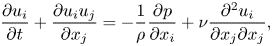 \begin{gather}\frac{\partial u_{i}}{\partial t} +\frac{\partial u_{i}u_{j}}{\partial x_{j}} ={-}\frac{1}{\rho}\frac{\partial p}{\partial x_{i}} +\nu\frac{\partial^{2} u_{i}}{\partial x_{j}\partial x_{j}}, \end{gather}
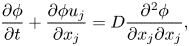 \begin{gather}\frac{\partial \phi}{\partial t} +\frac{\partial \phi u_{j}}{\partial x_{j}} = D\frac{\partial^{2} \phi}{\partial x_{j}\partial x_{j}}, \end{gather}
where  $u_{i}$ is the $i$th component of the velocity vector, $p$ is the pressure and $\rho$ is a constant value of the fluid density. These equations are solved with the DNS code based on the fractional step method. Periodic boundary conditions are applied in the $x$ and $z$ directions. The boundaries in the $y$ direction are treated with free-slip boundary conditions. Spatial derivatives are computed with fully conservative central difference schemes (Morinishi et al. Reference Morinishi, Lund, Vasilyev and Moin1998), where the second-order and fourth-order schemes are used in the lateral direction and other directions, respectively. Time is advanced with a third-order Runge–Kutta method. The Bi-CGSTAB method is used to solve the Poisson equation for pressure.
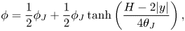
The initial mean velocity profile of the temporally evolving turbulent planar jet is given by a hyperbolic tangent function (da Silva & Pereira Reference da Silva and Pereira2008):
 \begin{equation} \langle {u}\rangle =\frac{1}{2}U_{J}+\frac{1}{2}U_{J}\tanh\left(\frac{H-2|y|}{4\theta_{J}}\right),\quad\langle v\rangle =\langle w\rangle =0, \end{equation}
with  $\theta _{J}=0.01H$. The centre of the jet is located at $y=0$. The initial velocity field consists of the mean velocity and spatially correlated random fluctuations (Watanabe et al. Reference Watanabe, Zhang and Nagata2019), where fluctuations with r.m.s. values of $0.025U_J$ are added in the region of $|y|\leqslant 0.5H$. The initial profile of $\phi$ is given by
 \begin{equation} \phi =\frac{1}{2}\phi_{J}+\frac{1}{2}\phi_{J}\tanh\left(\frac{H-2|y|}{4\theta_{J}}\right), \end{equation}
where  $\phi =\phi _J$ and 0 in the jet and ambient fluid, respectively. The DNS code solves the governing equations non-dimensionalized by $U_J$, $H$ and $\phi _J$.
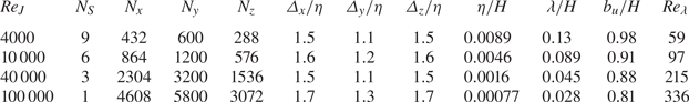
The DNS uses the computational domain with a size of  $(L_{x}\times L_{y}\times L_{z})=(6H\times 10H\times 4H)$. In a temporally evolving planar jet with this computational domain, the longitudinal autocorrelation function defined with the streamwise separation distance is consistent with DNS results of a spatially evolving turbulent planar jet as reported in Watanabe et al. (Reference Watanabe, Zhang and Nagata2019). Therefore, the computational domain is large enough to prevent unphysical effects of the periodic boundary conditions applied in the streamwise direction. A summary of the DNS is presented in table 1, which contains the number of grid points $(N_{x}\times N_{y}\times N_{z})$. The grid points are uniformly spaced in the $x$ and $z$ directions, while the grid is stretched in the $y$ direction as $|y|$ increases using a mapping function given by
 \begin{equation} y(\,j)={-}\frac{L_{y}}{2\alpha_y} {\mathrm{atanh}} \left[\left(\tanh\alpha_{y}\right) \left(1-2 \left(\frac{j-1}{N_y-1} \right) \right) \right]\quad \mathrm{with}\ j=1,\ldots,N_{y}, \end{equation}
with the grid stretching parameter  $\alpha _{y}=1.5$. In each simulation, time $t$ is advanced until $t=20t_r$, where $t_r=H/U_J$ is the reference time scale of the jet. The turbulent jet has fully developed by this time as examined below. The DNS for each $Re_J$ is repeated $N_S$ times with different initial velocity fluctuations, where $N_S$ is provided in table 1. Ensemble averages are taken for $N_S$ simulations to improve statistical convergence. As shown below, the shear layers are small-scale structures, whose length scale decreases with $Re_J$, and the number density of shear layers increases with the Reynolds number. Therefore, the number of statistical samples in the shear layer analysis in one simulation decreases as $Re_J$ becomes small. For this reason, $N_S$ is larger for lower-Reynolds-number cases. Parameter $N_S$ is determined such that the mean velocity profile around shear layers examined in § 4.3 is well converged.
Table 1. Computational and physical parameters of DNS. The statistics shown in the table are taken at  $t=20t_r$. Parameters $\varDelta _y$, $\eta$, $\lambda$ and $Re_\lambda$ are obtained at $y=0$.
2.2. Characteristics of the temporally evolving turbulent planar jet
Figure 1 visualizes the development of the planar jet at  $Re_J=4000$ and 40 000 with two-dimensional profiles of $\phi$ at four time instances. Turbulence is generated at the edges of the jet at $t=5t_r$ and spreads in the lateral direction with time. The jet core region has $\phi /\phi _J=1$ at early time while the jet development is accompanied by the mixing of the jet and ambient fluids, which results in $\phi /\phi _J<1$ even in the central region of the jet at late time. The jet has already fully developed at $t=15t_r$ as attested by small-scale scalar fluctuations that occupy the entire jet region. Although the initial mean velocity profile is the same in all simulations, the turbulent transition of the planar jet depends on the Reynolds number. At $Re_J=40\,000$, small-scale fluctuations exist inside the roller vortices arising from the Kelvin–Helmholtz instability in figure 1(f) while they are absent at $Re_J=4000$ in figure 1(b). We have also confirmed that pairing of multiple roller vortices occurs before $t/t_r=5$ at $Re_J=4000$ (not shown in figure 1). Then, as the roller vortices grow with time, the interaction of the vortices on both sides of the jet results in the formation of the fully developed turbulent jet. However, three-dimensional velocity and scalar fluctuations already develop inside the roller vortices at $Re_J=40\,000$, and turbulent mixing layers are formed at the edges of the jet before the turbulent jet develops. Then, the growth of the turbulent mixing layers results in the development of the turbulent jet at high $Re_J$.
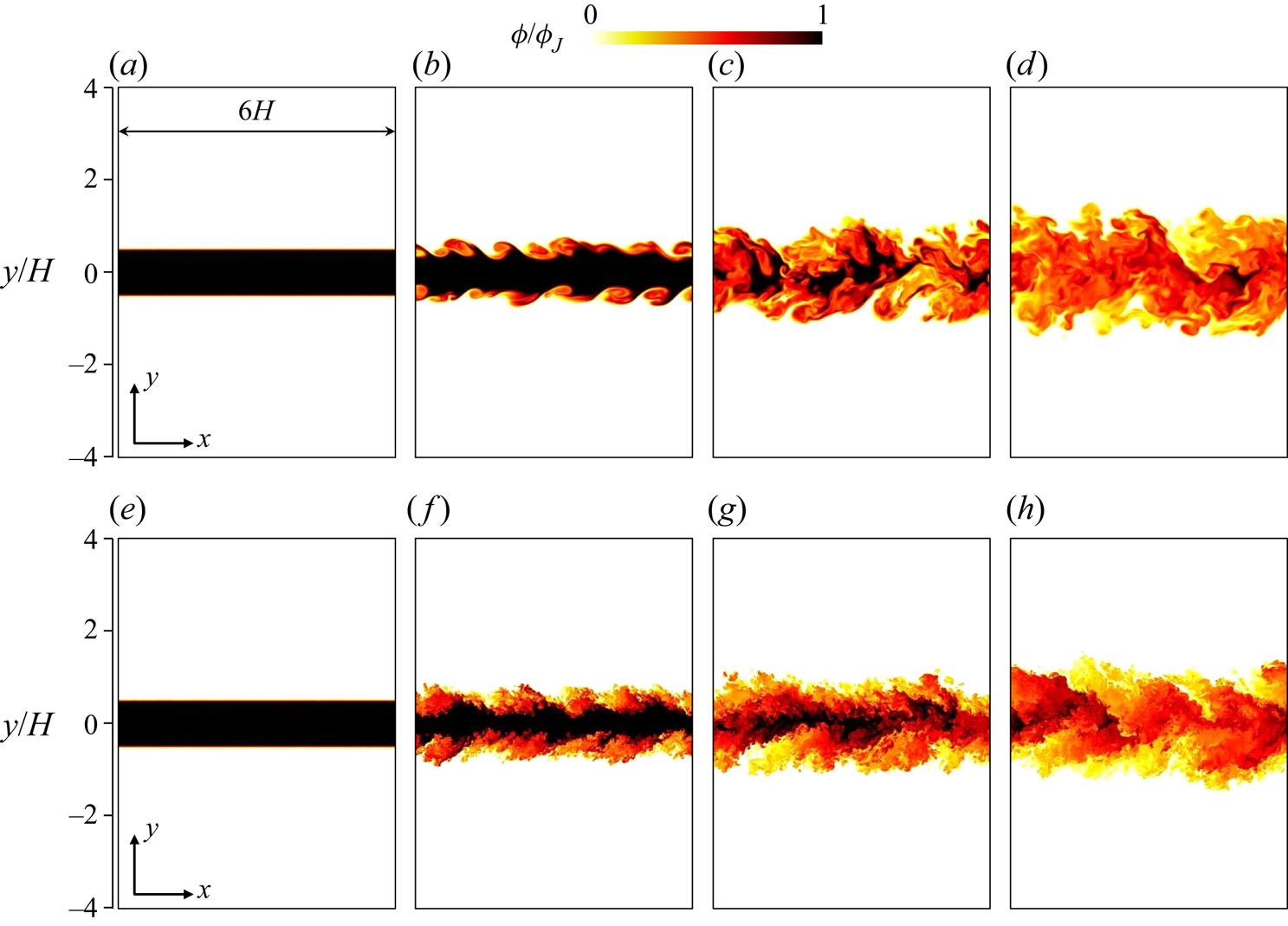
Figure 1. Development of the temporally evolving turbulent planar jet with (a–d)  $Re_J=4000$ and (e–h) $Re_J=40\,000$. Passive scalar $\phi$ is visualized on an $x$–
$x$– $y$ plane at (a,e) $t/t_r=0$, (b,f) $t/t_r=5$, (c,g) $t/t_r=10$ and (d,h) $t/t_r=15$.
Figure 2 shows the lateral profiles of mean streamwise velocity  $\langle u\rangle$ and r.m.s. streamwise velocity fluctuations $u_{rms}=\sqrt {\langle u^{2}\rangle -\langle u\rangle ^{2}}$ normalized by the mean centreline velocity $\langle u\rangle _{y0}$. The lateral position $y$ is normalized by the jet half-width $b_u$ defined with the mean streamwise velocity. The figure also includes the results of DNS and experiments of spatially evolving planar jets. Both mean velocity and r.m.s. velocity fluctuations in the present DNS agree well with previous studies, and the jet has reached a fully developed turbulent state at $t=20t_r$. The maximum value of $u_{rms}/\langle u\rangle _{y0}$ is away from the centreline. The peak value of $u_{rms}/\langle u\rangle _{y0}$ and its location $y/b_u$ vary between $0.23$ and $0.31$ and between $0.32$ and $0.81$, respectively, among the results of the spatially evolving jet shown in figure 2(b). The peak values in the present DNS are $0.26$, 0.25, 0.26 and 0.28 for $Re=4000$, 10 000, 40 000 and 100 000, respectively, while the peak locations for these $Re_J$ values are $y/b_u=0.76$, $0.87$, $0.78$ and $0.77$. The peaks and locations are within the variations among the previous studies.

Figure 2. Lateral profiles of (a) mean streamwise velocity  $\langle u\rangle$ and (b) r.m.s. streamwise velocity fluctuations $u_{rms}$. Here $\langle u\rangle$ and $u_{rms}$ are normalized by the mean centreline velocity $\langle u\rangle _{y0}$ and the lateral coordinate $y$ is normalized by the jet half-width defined with $\langle u\rangle$. The DNS results are compared with previous experiments and DNS of spatially evolving planar jets, where the legend also presents the streamwise location $x/H$ and the Reynolds number $Re_J$ (Gutmark & Wygnanski Reference Gutmark and Wygnanski1976; Namer & Ötügen Reference Namer and Ötügen1988; Stanley, Sarkar & Mellado Reference Stanley, Sarkar and Mellado2002; Klein, Sadiki & Janicka Reference Klein, Sadiki and Janicka2003; Deo, Mi & Nathan Reference Deo, Mi and Nathan2008; Deo, Nathan & Mi Reference Deo, Nathan and Mi2013; Terashima, Sakai & Nagata Reference Terashima, Sakai and Nagata2012; Watanabe et al. Reference Watanabe, Sakai, Nagata, Ito and Hayase2014b,Reference Watanabe, Sakai, Nagata and Terashimac; da Silva, Lopes & Raman Reference da Silva, Lopes and Raman2015; Takahashi et al. Reference Takahashi, Iwano, Sakai and Ito2019; Matsubara, Alfredsson & Segalini Reference Matsubara, Alfredsson and Segalini2020).
Variations of  $u_{rms}/U_J$ among experiments and numerical simulations are possibly explained by the inflow conditions at the nozzle. As shown in figure 1, the Reynolds number is important in the shear layer development at the edges of the jet, and the $Re$ dependence of the initial shear layers can affect the properties of the fully developed turbulent planar jet. In the present study, the initial shear layers have Reynolds number $Re_\theta =U_J \theta _J/\nu$, where $\theta _{J}=0.01H$ is assumed in (2.4a,b). Reynolds number $Re_\theta =0.01Re_J$ is 40 for $Re_J=4000$ and 1000 for $Re_J=100\,000$, and the viscous effects during the shear instability can be important for $Re_J=4000$. For example, the initial velocity fluctuations decay faster at a lower Reynolds number before the transition, and the actual fluctuations that trigger the transition can depend on $Re_J$ ( $Re_\theta$). The mean velocity profile at the nozzle is also different among experiments and numerical simulations. Some experiments used a skimmer to eliminate the boundary layers that develop inside the nozzle (Terashima et al. Reference Terashima, Sakai and Nagata2012; Takahashi et al. Reference Takahashi, Iwano, Sakai and Ito2019). The inflow mean velocity in this case is well described by a top-hat profile (Terashima, Sakai & Ito Reference Terashima, Sakai and Ito2018), which corresponds to (2.4a,b) with very small $\theta _{J}$. If a skimmer is not used in experiments, the inflow velocity is influenced by the boundary layers inside a nozzle (Deo et al. Reference Deo, Mi and Nathan2008; Watanabe et al. Reference Watanabe, Sakai, Nagata, Ito and Hayase2014a; Matsubara et al. Reference Matsubara, Alfredsson and Segalini2020). Even if the jet Reynolds numbers are identical in these experiments, the Reynolds numbers of the initial shear layers are different depending on the usage of the skimmer and the shape of the nozzle. Wu et al. (Reference Wu, Sakai, Nagata, Suzuki, Terashima and Hayase2013) tested top-hat and parabolic profiles of the mean inflow velocity in DNS of a spatially evolving planar jet, and found that the evolution of velocity statistics is different for these profiles. The turbulent intensity defined as $u_{rms}/U_J$ at the nozzle exit was also different among experiments and simulations. In experiments, $u_{rms}/U_J$ at the centre of the nozzle was about 0.01 in Deo et al. (Reference Deo, Mi and Nathan2008), 0.012 in Terashima et al. (Reference Terashima, Sakai and Nagata2012) and 0.05 in Watanabe et al. (Reference Watanabe, Sakai, Nagata, Ito and Hayase2014a) while the profile of $u_{rms}/U_J$ inside the nozzle is very different among these experiments. It was shown that the velocity fluctuations at the nozzle exit also affect jet development (Klein et al. Reference Klein, Sadiki and Janicka2003). Watanabe et al. (Reference Watanabe, Sakai, Nagata, Ito and Hayase2014a) conducted DNS of a spatially evolving planar jet with the profiles of mean velocity and r.m.s. streamwise velocity fluctuations measured in the experimental apparatus used in Watanabe et al. (Reference Watanabe, Sakai, Nagata and Terashima2014c). The evolution of first- and second-order statistics of velocity and passive scalar (dye concentration) was in excellent agreement between the DNS and experiment. These results indicate the importance of inflow velocity characteristics in the statistics of the fully developed turbulent jet. The r.m.s. velocity fluctuations are dominated by large-scale velocity fluctuations. The DNS of a temporally evolving planar jet confirmed that the initial velocity profile affects the shape of large-scale vortices visualized by pressure isosurface (Taveira & da Silva Reference Taveira and da Silva2013). That DNS suggested that the initial roller vortices at the edges of the jet sometimes persist even at late time. Numerical simulations of turbulent mixing layers also found that the roller vortices of the Kelvin–Helmholtz instability can persist even in the self-similar region depending on the initial conditions, and the presence of the vortices affects the statistics in the self-similar region (Balaras, Piomelli & Wallace Reference Balaras, Piomelli and Wallace2001). Similarly, the influence of the inflow velocity on the fully developed turbulent jet can also be related to the large-scale vortices in the jet.
The DNS databases at  $t=20t_r$ are analysed in this study. Table 1 also includes the Kolmogorov length scale $\eta =(\nu ^{3}/\varepsilon )^{1/4}$, Taylor microscale $\lambda =\sqrt {15\nu u_0^{2}/\varepsilon }$, jet half-width $b_u$ and turbulent Reynolds number $Re_{\lambda }=u_0 \lambda /\nu$ at $t=20t_r$, where $\varepsilon =2\nu \langle {\mathsf{S}}_{ij}{\mathsf{S}}_{ij}\rangle$ is the mean kinetic energy dissipation rate and $u_0=\sqrt {(u_{rms}^{2}+v_{rms}^{2}+w_{rms}^{2})/3}$ is the characteristic velocity scale of energy-containing, large-scale motions. Here, $\eta$, $\lambda$ and $Re_{\lambda }$ are taken at the centre of the jet ( $y=0$). The spatial resolution in each direction $\varDelta _i$ is compared with the Kolmogorov length scale at $y=0$, and $\varDelta _x=\varDelta _z\approx 1.6\eta$ and $\varDelta _y\approx 1.2\eta$ are small enough for the present central difference schemes to resolve small-scale fluctuations (Watanabe et al. Reference Watanabe, Riley, Nagata, Onishi and Matsuda2018a).
The turbulent jet is known as an intermittent turbulent flow, where both turbulent and non-turbulent fluids appear at a given location. The turbulent fluid is separated from the non-turbulent fluid by a thin interface (da Silva et al. Reference da Silva, Hunt, Eames and Westerweel2014). In this study, the characteristics of shear layers are compared with the length and velocity scales of turbulence. As these scales are different between turbulent and non-turbulent regions, the scales are estimated solely from the turbulent region as functions of  $y$. The turbulent region of the planar jet can be detected with vorticity magnitude $\omega =|\boldsymbol {\omega }|$ (Bisset, Hunt & Rogers Reference Bisset, Hunt and Rogers2002). Here, we define turbulent and non-turbulent fluids as $\omega \geqslant \omega _{th}$ and $\omega < \omega _{th}$, respectively, with a threshold $\omega _{th}$. An appropriate value of $\omega _{th}$ is determined by $\omega _{th}$ dependence of the detected turbulent volume $V_T$ following Taveira et al. (Reference Taveira, Diogo, Lopes and da Silva2013). Figure 3(a) shows the relation between $V_T(\omega _{th})$ and $\omega _{th}/\langle \omega \rangle _{y0}$ for $Re_J=10\,000$, where $\langle \omega \rangle _{y0}$ is the mean vorticity magnitude on the jet centreline and $V_T$ is defined as the volume normalized by $H^{3}$. As $\omega _{th}/\langle \omega \rangle _{y0}$ decreases from $10^{1}$ to $10^{-1}$, $V_T$ increases because the turbulent fluid with large $\omega$ is detected. Then, $V_T$ slowly varies with the threshold for $10^{-4} \lesssim \omega _{th}/\langle \omega \rangle _{y0}\lesssim 10^{-1}$. This is because the interfacial layer that separates the turbulent and non-turbulent regions occupies small volume in the flow (da Silva et al. Reference da Silva, Hunt, Eames and Westerweel2014). Then, $V_T$ begins to markedly increase as $\omega _{th}/\langle \omega \rangle _{y0}$ becomes smaller than $10^{-4}$. The turbulent region is well detected when $\omega _{th}/\langle \omega \rangle _{y0}$ is chosen in the range where $V_T$ weakly depends on $\omega _{th}/\langle \omega \rangle _{y0}$. This range is better appreciated by a plot of $V'_T=\textrm {d}V_T/\textrm {d}({\mathrm {log}}_{10}\omega _{th})$, which is also shown in figure 3(a). The inset shows the range of $\omega _{th}/\langle \omega \rangle _{y0}$ with small $-V'_T$, which has a local minimum at $\omega _{th}/\langle \omega \rangle _{y0}\approx 10^{-3}$. Very small $\omega$ in the non-turbulent region often arises from errors due to numerical schemes, and is detected as a turbulent region if the threshold $\omega _{th}/\langle \omega \rangle _{y0}$ is smaller than $10^{-3}$. For $\omega _{th}/\langle \omega \rangle _{y0}\gtrsim 10^{-2}$, $-V'_T$ begins to rapidly increase with $\omega _{th}$. Therefore, the threshold can be chosen from $10^{-3}\lesssim \omega _{th}/\langle \omega \rangle _{y0}\lesssim 10^{-2}$. Figure 3(b) shows the isolines of $\omega =\omega _{th}$ with $\omega _{th}=0.01\langle \omega \rangle _{y0}$, $0.006\langle \omega \rangle _{y0}$ and $0.002\langle \omega \rangle _{y0}$ near the outer edge of the jet. The contour is the logarithmic plot of enstrophy $\omega ^{2}/2$. Regions with large $\omega ^{2}/2$ (shown with red colour) are considered as vortex tubes (Jiménez et al. Reference Jiménez, Wray, Saffman and Rogallo1993), whose diameter is about 10 times the Kolmogorov scale near the turbulent–non-turbulent interface (TNTI) layer in a temporally evolving planar jet (Watanabe et al. Reference Watanabe, da Silva, Nagata and Sakai2017). The isoline location slightly changes for the three thresholds. However, this change is much smaller than the size of large-enstrophy regions. In the rest of the paper, the turbulent region is detected with $\omega _{th}=0.01\langle \omega \rangle _{y0}$. As $\langle \omega \rangle _{y0}$ varies with time and is also different depending on $Re_J$, the threshold is not a constant. Previous studies also used the threshold that varies with the streamwise location (time) of spatially (temporally) evolving turbulent flows (Bisset et al. Reference Bisset, Hunt and Rogers2002; Attili, Cristancho & Bisetti Reference Attili, Cristancho and Bisetti2014; Watanabe et al. Reference Watanabe, Sakai, Nagata, Ito and Hayase2014b; Zhou & Vassilicos Reference Zhou and Vassilicos2017; Watanabe et al. Reference Watanabe, Zhang and Nagata2019). If the resolution of DNS is not good enough, the well-defined interface is not detected with the isosurface of $\omega$. It was shown that a low resolution causes unphysical vorticity oscillation in the concave region of the interface (concave in the view from the non-turbulent region), and the isosurface of $\omega$ becomes partially jagged (Watanabe et al. Reference Watanabe, Zhang and Nagata2018b). For the present DNS code, this unphysical vorticity oscillation becomes noticeably large for $\varDelta _i\gtrsim 2\eta$ (Watanabe et al. Reference Watanabe, Zhang and Nagata2018b). The isoline in figure 3(b) is smooth even in the concave region, and the present DNS does not have the resolution issue for interface detection.
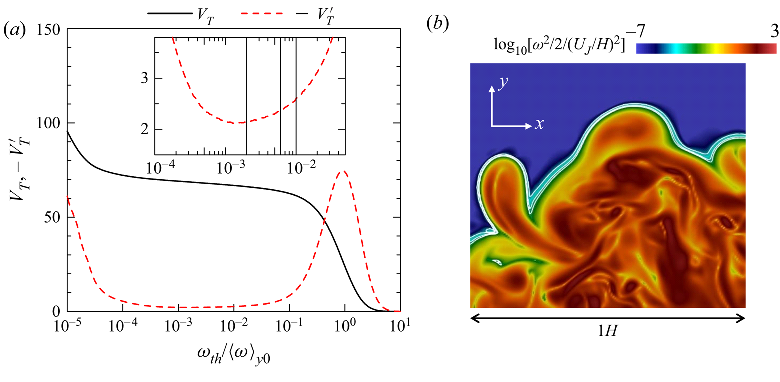
Figure 3. (a) Turbulent volume  $V_T$ and $-V_T'=-\textrm {d}V_T/\textrm {d}(\mathrm {log}_{10}\omega _{th})$ plotted against the detection threshold $\omega _{th}$. The vertical lines in the inset represent $\omega _{th}$ visualized in (b). (b) Logarithmic contour of enstrophy $\omega ^{2}/2$ and isoline of $\omega =\omega _{th}$ on an $x$–
$x$– $y$ plane with $\omega _{th}=0.01\langle \omega \rangle _{y0}$, $0.006\langle \omega \rangle _{y0}$ and $0.002\langle \omega \rangle _{y0}$. These results are obtained in DNS for $Re=10\,000$.
We define an intermittency function  $I(x,y,z)$, which is equal to 1 for $\omega (x,y,z)\geqslant \omega _{th}$ and to 0 for $\omega (x,y,z)<\omega _{th}$. An average of a variable $f$ in the turbulent region is defined as $\langle \,f\rangle _T\equiv \langle I f\rangle / \langle I \rangle$ (LaRue & Libby Reference LaRue and Libby1974), which is obtained as a function of $y$ at each time instance. The r.m.s. velocity fluctuations in three directions are calculated as $u_{rmsT}=(\langle u^{2}\rangle _T - \langle u\rangle _T^{2})^{1/2}$, $v_{rmsT}=(\langle v^{2}\rangle _T - \langle v\rangle _T^{2})^{1/2}$ and $w_{rmsT}=(\langle w^{2}\rangle _T - \langle w\rangle _T^{2})^{1/2}$. The characteristic velocity and length scales of large-scale motions in the turbulent region are defined as
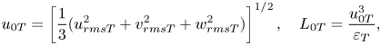 \begin{equation} u_{0T}= \left[\frac{1}{3}(u_{rmsT}^{2}+ v_{rmsT}^{2}+ w_{rmsT}^{2})\right]^{1/2},\quad L_{0T} =\frac{u_{0T}^{3}}{\varepsilon_T}, \end{equation}
respectively, where  $\varepsilon _T=2\nu \langle {\mathsf{S}}_{ij}{\mathsf{S}}_{ij}\rangle _T$ is the kinetic energy dissipation rate averaged for the turbulent fluids. Similarly, the Kolmogorov velocity and length scales in turbulence are defined as
 \begin{equation} u_{\eta T}=(\nu \varepsilon_T)^{1/4},\quad \eta_T=(\nu^{3}/\varepsilon_T)^{1/4}, \end{equation}
respectively.
Figure 4(a) shows an intermittency factor  $\gamma =\langle I\rangle$, which is a probability that turbulent fluid is found at $y$. As confirmed from $\gamma =1$ for $y/b_u\lesssim 1$, the region near the jet centreline is always turbulent. On the other hand, $\gamma$ decreases with $y$ for $y/b_u\gtrsim 1$, where the non-turbulent region also exists intermittently. The profile of $\gamma$ in the DNS agrees with experimental results of a spatially evolving planar jet. Figure 4(b,c) compares the velocity and length scales defined with conventional averages $\langle \ \rangle$ and averages of the turbulent fluids $\langle \ \rangle _T$, where the statistics calculated with $\langle \ \rangle _T$ are shown for $y$ with $\gamma \geqslant 0.05$. Here, the integral scale is defined as $L_{0} = u_{0}^{3}/\varepsilon$ (Pope Reference Pope2000). In the region with $\gamma =1$, the length and velocity scales are identical for both averages. However, these averages are different in the intermittent region with $\gamma <1$. This is because the non-turbulent region has different characteristic length and velocity scales from the turbulent region. As the shear layers appear only in the turbulent region, the characteristics of shear layers are compared with the velocity and length scales defined with averages of the turbulent fluids. Figure 5 shows the temporal evolution of the length scales $L_{0}$, $\lambda$ and $\eta$ at $y=0$ for $Re_J=4000$. These length scales rapidly change with time during the turbulent transition ( $t_r\lesssim 10$), and slowly increase at a later time. All results presented in this paper are taken at $t/t_r=20$.

Figure 4. Lateral profiles of (a) intermittency factor  $\gamma$, (b) integral length scale and Kolmogorov length scale and (c) characteristic velocity scale of large-scale motions and Kolmogorov velocity scale at $t=20t_r$ in DNS for $Re_J=10\,000$. The intermittency factor is compared with experimental data measured at the streamwise distance from the jet nozzle of $x/H=20$ and $40$ in a turbulent planar jet with $Re_J=2200$ (Watanabe et al. Reference Watanabe, Naito, Sakai, Nagata and Ito2015). (b,c) Comparison of length and velocity scales defined with conventional averages ( $L_{0}$, $\eta$, $u_{0}$ and $u_\eta$) and averages of turbulent fluids ( $L_{0T}$, $\eta _T$, $u_{0T}$ and $u_{\eta T}$).
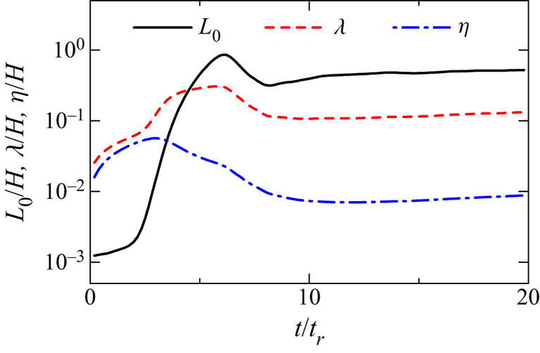
Figure 5. Temporal evolution of length scales  $L_{0}$, $\lambda$ and $\eta$ on the jet centreline ( $Re_J=4000$).
3. Shear layer analysis based on the triple decomposition of the velocity gradient tensor
3.1. Triple decomposition of the velocity gradient tensor
The triple decomposition of the velocity gradient tensor (Kolář Reference Kolář2007; Watanabe et al. Reference Watanabe, Tanaka and Nagata2020) is applied to the DNS databases described above. The triple decomposition decomposes the velocity gradient tensor  $\boldsymbol {\nabla }{\boldsymbol {u}}$ into three components which represent the motions of shear ( $S$), rotation ( $R$) and elongation ( $E$) as $\boldsymbol {\nabla } {\boldsymbol {u}}=\boldsymbol {\nabla } {\boldsymbol {u}}_{S}+\boldsymbol {\nabla } {\boldsymbol {u}}_{R}+\boldsymbol {\nabla } {\boldsymbol {u}}_{E}$. In the triple decomposition, the shear tensor $\boldsymbol {\nabla } {\boldsymbol {u}}_{S}$ is extracted from $\boldsymbol {\nabla } {\boldsymbol {u}}$ as
 \begin{align} (\boldsymbol{\nabla} {\boldsymbol{u}}_{S})_{ij}= \begin{cases} (\boldsymbol{\nabla} {\boldsymbol{u}})_{ij} -\mathrm{sgn}[(\boldsymbol{\nabla} {\boldsymbol{u}})_{ij}] \mathrm{min}[|(\boldsymbol{\nabla} {\boldsymbol{u}})_{ij}|,|(\boldsymbol{\nabla} {\boldsymbol{u}})_{ji}|] & \mathrm{for}\ (i,j)=(1,2)\ \mathrm{and}\ (1,3) \\ 0 & \mathrm{otherwise}, \end{cases} \end{align}
where  $\mathrm {sgn}(x)$ is the sign function. Then, $\boldsymbol {\nabla } {\boldsymbol {u}}_{E}$ and $\boldsymbol {\nabla } {\boldsymbol {u}}_{R}$ are obtained respectively as symmetric and antisymmetric parts of the residual tensor $(\boldsymbol {\nabla } {\boldsymbol {u}}_{RES})_{ij}=(\boldsymbol {\nabla } {\boldsymbol {u}})_{ij}-(\boldsymbol {\nabla } {\boldsymbol {u}}_{S})_{ij}$:
 \begin{gather} (\boldsymbol{\nabla} {\boldsymbol{u}}_{E})_{ij}=[(\boldsymbol{\nabla} {\boldsymbol{u}}_{RES})_{ij}+( \boldsymbol{\nabla} {\boldsymbol{u}}_{RES})_{ji}]/2, \end{gather}
 \begin{gather}(\boldsymbol{\nabla} {\boldsymbol{u}}_{R})_{ij}=[ (\boldsymbol{\nabla} {\boldsymbol{u}}_{RES})_{ij} -(\boldsymbol{\nabla} {\boldsymbol{u}}_{RES})_{ji}]/2. \end{gather}
Equation (3.1) ensures that  $\boldsymbol {\nabla } {\boldsymbol {u}}_{S}$ represents a simple shear. However, the application of (3.1) does not always extract the shearing motion of the flow. In the triple decomposition, (3.1) must be applied in a specific frame of reference where (3.1) can effectively extract the shearing motion (Kolář Reference Kolář2007). This reference frame is called a basic reference frame, which is identified by a method described in Appendix A. The basic reference frame assumes that the shearing motion extracted by (3.1) is the strongest in the basic reference frame among all reference frames. The decomposition applied in the basic reference frame provides $\boldsymbol {\nabla } {\boldsymbol {u}}_{S}$, $\boldsymbol {\nabla } {\boldsymbol {u}}_{R}$ and $\boldsymbol {\nabla } {\boldsymbol {u}}_{E}$ in this frame. These tensors in the original coordinates $(x,y,z)$ are obtained with the coordinate transformation tensor from the basic reference frame to $(x,y,z)$ defined in Appendix A.
The basic reference frame is locally determined at each grid point, where the decomposition given by (3.1)–(3.3) provides three decomposed tensors. The triple decomposition is repeatedly applied in the entire computational domain of the DNS databases to obtain the three-dimensional data of  $\boldsymbol {\nabla } {\boldsymbol {u}}_{S}$, $\boldsymbol {\nabla } {\boldsymbol {u}}_{R}$ and $\boldsymbol {\nabla } {\boldsymbol {u}}_{E}$. Intensities of shear, rotation and elongation are evaluated as $I_S=\sqrt {2(\boldsymbol {\nabla } {\boldsymbol {u}}_{S})_{ij}(\boldsymbol {\nabla } {\boldsymbol {u}}_{S})_{ij}}$, $I_R=\sqrt {2(\boldsymbol {\nabla } {\boldsymbol {u}}_{R})_{ij}(\boldsymbol {\nabla } {\boldsymbol {u}}_{R})_{ij}}$ and $I_E=\sqrt {2(\boldsymbol {\nabla } {\boldsymbol {u}}_{E})_{ij}(\boldsymbol {\nabla } {\boldsymbol {u}}_{E})_{ij}}$, respectively.
3.2. Analysis of shear layers
Shear layers can be detected as regions with large  $I_S$ (Eisma et al. Reference Eisma, Westerweel, Ooms and Elsinga2015; Nagata et al. Reference Nagata, Watanabe, Nagata and da Silva2020). The shear layers in the planar jet are investigated with the method proposed in Watanabe et al. (Reference Watanabe, Tanaka and Nagata2020), which examines the flow field around local maxima of $I_S$. When flow structures associated with shearing motion are identified in a three-dimensional profile of $I_S$, one can find at least one local maximum of $I_S$ in the structure. Here, the local maxima can be found with a Hessian matrix of $-I_S$ defined as ${\mathsf{H}}_{ij}=-\partial ^{2} I_S / \partial x_i \partial x_j$. We denote a variable $f$ at an orthogonal grid point $(i,j,k)$ by $f^{(i,j,k)}$ and the spatial derivative of $f$ by $\partial _{x_i} f=\partial f/\partial x_i$, where $(i,j,k)$ represents the location of grid points in $x$,
$x$,  $y$ and $z$ directions. Local maxima of $I_S$ used for the analysis of the shear layers are identified as grid points ( $i,j,k$) that satisfy the following conditions:
 \begin{gather} (\partial_{x} I_S)^{(i-1,j,k)}(\partial_{x} I_S)^{(i+1,j,k)}<0, \end{gather}
 \begin{gather} (\partial_{y} I_S)^{(i,j-1,k)}(\partial_{y} I_S)^{(i,j+1,k)}<0, \end{gather}
 \begin{gather} (\partial_{z} I_S)^{(i,j,k-1)}(\partial_{z} I_S)^{(i,j,k+1)}<0, \end{gather}
 \begin{gather}
{\mathsf{H}}_{11}^{(i,j,k)}>0, \quad
({\mathsf{H}}_{11}{\mathsf{H}}_{22}-{\mathsf{H}}_{12}{\mathsf{H}}_{21})^{(i,j,k)}>0,
\end{gather}
\begin{gather}
{\mathsf{H}}_{11}^{(i,j,k)}>0, \quad
({\mathsf{H}}_{11}{\mathsf{H}}_{22}-{\mathsf{H}}_{12}{\mathsf{H}}_{21})^{(i,j,k)}>0,
\end{gather}
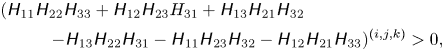 \begin{gather}
\hspace{-8pc}({\mathsf{H}}_{11}{\mathsf{H}}_{22}{\mathsf{H}}_{33} + {\mathsf{H}}_{12}{\mathsf{H}}_{23}H_{31} +
{\mathsf{H}}_{13}{\mathsf{H}}_{21}{\mathsf{H}}_{32}\nonumber\\
\hspace{-8pc}\qquad\quad\qquad\qquad\qquad\qquad - {\mathsf{H}}_{13}{\mathsf{H}}_{22}{\mathsf{H}}_{31} - {\mathsf{H}}_{11}{\mathsf{H}}_{23}{\mathsf{H}}_{32} -
{\mathsf{H}}_{12}{\mathsf{H}}_{21}{\mathsf{H}}_{33})^{(i,j,k)}>0,\end{gather}
\begin{gather}
\hspace{-8pc}({\mathsf{H}}_{11}{\mathsf{H}}_{22}{\mathsf{H}}_{33} + {\mathsf{H}}_{12}{\mathsf{H}}_{23}H_{31} +
{\mathsf{H}}_{13}{\mathsf{H}}_{21}{\mathsf{H}}_{32}\nonumber\\
\hspace{-8pc}\qquad\quad\qquad\qquad\qquad\qquad - {\mathsf{H}}_{13}{\mathsf{H}}_{22}{\mathsf{H}}_{31} - {\mathsf{H}}_{11}{\mathsf{H}}_{23}{\mathsf{H}}_{32} -
{\mathsf{H}}_{12}{\mathsf{H}}_{21}{\mathsf{H}}_{33})^{(i,j,k)}>0,\end{gather} \begin{gather} \mathrm{sgn}[(\partial_{x}I_S)^{(i-1,j,k)}] =\mathrm{sgn}[(\partial_{x}I_S)^{(i-2,j,k)}] =\mathrm{sgn}[(\partial_{x}I_S)^{(i-3,j,k)}], \end{gather}
 \begin{gather}\mathrm{sgn}[(\partial_{y}I_S)^{(i,j-1,k)}] =\mathrm{sgn}[(\partial_{y}I_S)^{(i,j-2,k)}] =\mathrm{sgn}[(\partial_{y}I_S)^{(i,j-3,k)}], \end{gather}
 \begin{gather}\mathrm{sgn}[(\partial_{z}I_S)^{(i,j,k-1)}] =\mathrm{sgn}[(\partial_{z}I_S)^{(i,j,k-2)}] =\mathrm{sgn}[(\partial_{z}I_S)^{(i,j,k-3)}], \end{gather}
 \begin{gather}\mathrm{sgn}[(\partial_{x}I_S)^{(i+1,j,k)}] =\mathrm{sgn}[(\partial_{x}I_S)^{(i+2,j,k)}] =\mathrm{sgn}[(\partial_{x}I_S)^{(i+3,j,k)}], \end{gather}
 \begin{gather}\mathrm{sgn}[(\partial_{y}I_S)^{(i,j+1,k)}] =\mathrm{sgn}[(\partial_{y}I_S)^{(i,j+2,k)}] =\mathrm{sgn}[(\partial_{y}I_S)^{(i,j+3,k)}], \end{gather}
 \begin{gather}\mathrm{sgn}[(\partial_{z}I_S)^{(i,j,k+1)}] =\mathrm{sgn}[(\partial_{z}I_S)^{(i,j,k+2)}] =\mathrm{sgn}[(\partial_{z}I_S)^{(i,j,k+3)}]. \end{gather}
Equations (3.4)–(3.8) ensure that  $I_S$ attains a local maximum at $(i,j,k)$. Local maxima of $I_S$ can also appear in noise-like patterns of very small $I_S$, which are not related to the shear layer structures of turbulence. These points can be eliminated from the analysis with additional conditions (3.9)–(3.14). It was shown that these criteria successfully identify shear layers in isotropic turbulence in Watanabe et al. (Reference Watanabe, Tanaka and Nagata2020). Values of $I_S$ are different depending on flows and Reynolds numbers. However, the detection criterion given by (3.4)–(3.14) uses the sign of the gradient of $I_S$ and the location of the local maxima of $I_S$, and does not rely on the value of $I_S$ itself. Therefore, (3.4)–(3.14) are expected to be useful in shear layer detection in various turbulent flows.
We introduce a shear coordinate system  $(\zeta _1,\zeta _2,\zeta _3)$ for each point of local maxima of $I_S$ that satisfies (3.4)–(3.14). The orientations of $\zeta _1$, $\zeta _2$ and $\zeta _3$ are represented by unit vectors ${\boldsymbol {n}}_1$, ${\boldsymbol {n}}_2$ and ${\boldsymbol {n}}_3$, respectively. In the Cartesian coordinates used in the DNS, the unit vector ${\boldsymbol {n}}_i$ is expressed with three components as $(({\boldsymbol {n}}_i)_{x},({\boldsymbol {n}}_i)_{y},({\boldsymbol {n}}_i)_{z})$. The shear coordinate assumes that the shear is expressed with the derivative of ${\boldsymbol {n}}_3$-directional velocity with respect to $\zeta _2$ as illustrated in figure 6(a). The shear coordinate is identified with the method used in Watanabe et al. (Reference Watanabe, Tanaka and Nagata2020). First, ${\boldsymbol {n}}_1$ is determined as the direction of the vorticity vector of the shear tensor, ${\boldsymbol {n}}_1={\boldsymbol {\omega }}_{S}/|{\boldsymbol {\omega }}_{S}|$, with $({\boldsymbol {\omega }}_{S})_{i}= \epsilon _{ijk}(\boldsymbol {\nabla } {\boldsymbol {u}}_{S})_{jk}$, where $\epsilon _{ijk}$ is the Levi-Civita symbol. Then, ${\boldsymbol {n}}_2$ and ${\boldsymbol {n}}_3$ are determined so that the shear tensor $\boldsymbol {\nabla } {\boldsymbol {u}}_{S}$ satisfies the following relation in the shear coordinate:
 \begin{gather} (\boldsymbol{\nabla} {\boldsymbol{u}}_{S})_{ij}\neq 0 \quad \textrm{{for}}\ (i,j)=(3,2), \end{gather}
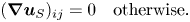 \begin{gather}(\boldsymbol{\nabla} {\boldsymbol{u}}_{S})_{ij}= 0 \quad \textrm{{otherwise}}. \end{gather}
Vectors  ${\boldsymbol {n}}_2$ and ${\boldsymbol {n}}_3$ are obtained with the method presented in Appendix B.
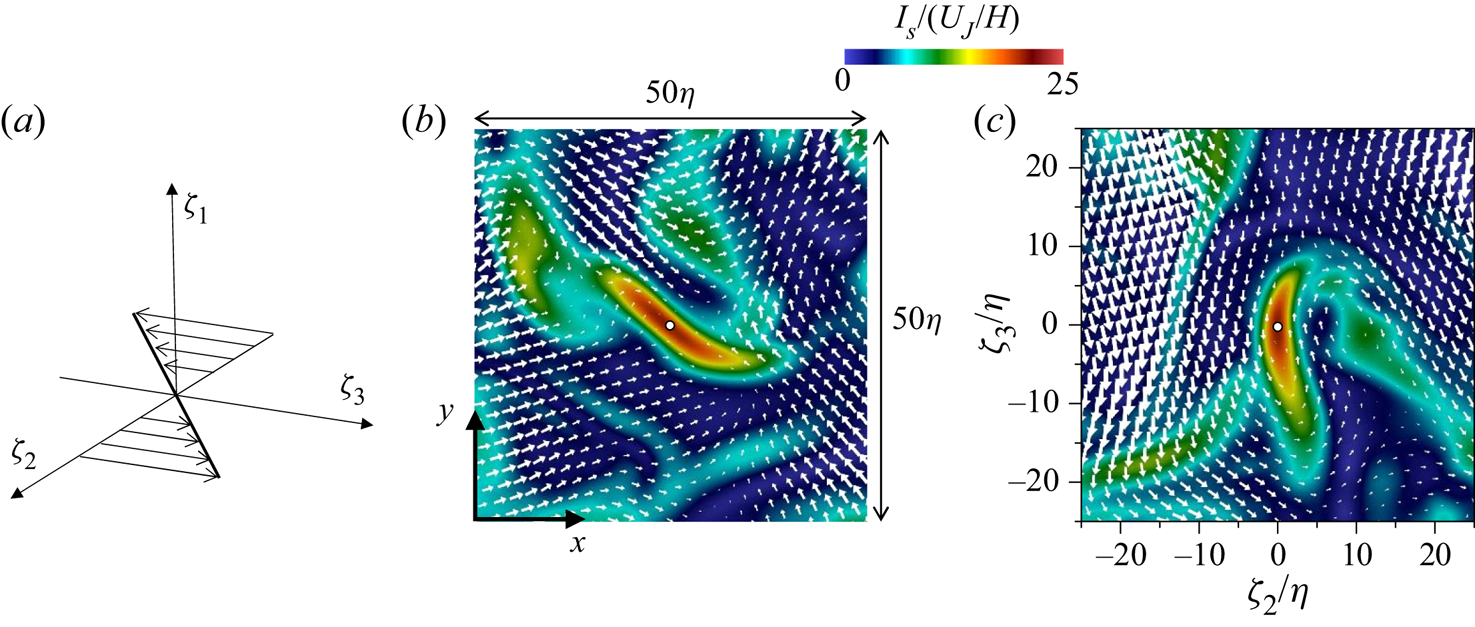
Figure 6. (a) Shear coordinate defined with a shear tensor  $\boldsymbol {\nabla } {\boldsymbol {u}}_{S}$. A flow field around a local maximum of $I_S$ used in the shear layer analysis: (b) $x$–
$x$– $y$ plane; (c) $\zeta _2$– $\zeta _3$ plane of the shear coordinate. The circle at the centre of each panel marks the location of the local maximum of $I_S$. The relative velocity with respect to the local maximum location of $I_S$ is shown on each plane.
Once the shear coordinate is identified for each local maximum of  $I_S$, flow variables on $(\zeta _1,\zeta _2,\zeta _3)$ are interpolated from the DNS grid by using a third-order Lagrange polynomial interpolation scheme. The relative velocity with respect to $(\zeta _1,\zeta _2,\zeta _3)=(0,0,0)$ is used in the present analysis, where $\zeta _1$, $\zeta _2$ and $\zeta _3$ components of the relative velocity are denoted by $u_1$, $u_2$ and $u_3$, respectively. Figure 6(b,c) shows a flow field around a local maximum of $I_S$ at $y=0$ of the jet with $Re_J=10\,000$. The shear layer is visualized as a thin region with large $I_S$. The velocity vector on the $x$–
$x$– $y$ plane does not show the shear layer pattern. However, after the coordinate transformation from $(x,y,z)$ to $(\zeta _1,\zeta _2,\zeta _3)$, the shear is well represented by the velocity in $\pm \zeta _3$ directions for $\zeta _2>0$ and $\zeta _2<0$ in figure 6(c). The coordinate transformaton from $(x,y,z)$ to $(\zeta _1,\zeta _2,\zeta _3)$ is applied at all local maxima of $I_S$ that satisfy (3.4)–(3.14). Ensemble averages of the interpolated variables are taken as functions of $(\zeta _1,\zeta _2,\zeta _3)$ with a large number of detected local maxima of $I_S$. This average is denoted by $\bar {f}$. Statistics in the temporally evolving turbulent planar jet depend on $y$ and time. Therefore, the ensemble averages at a given time step are also taken as functions of $y$, i.e. $\bar {f}(y; \zeta _1,\zeta _2,\zeta _3)$. As presented below, shearing motion hardly exists outside the jet, and the number of samples of the shear layers becomes very small near the outer edge of the jet. Therefore, the analysis of shear layers is conducted for $0\leqslant y\leqslant 2b_u$ because the turbulent fluid hardly appears beyond $y=2b_u$. Detected local maxima of $I_S$ are binned into 11 bins centred at $y/b_u=0, 0.2, 0.4,\ldots, 2.0$, where all bins have equal width of $0.2b_u$. The ensemble averages are taken with all local maxima of $I_S$ in each bin. For example, a local maximum of $I_S$ found at $y=0.25b_u$ is used as a sample of the statistics calculated at $y/b_u=0.2$.
4. Results and discussion
4.1. Flow visualization with tensors obtained by the triple decomposition
Figure 7 visualizes  $I_S$, $I_R$ and $I_E$ on an $x$–
$x$– $y$ plane of the planar jet with $Re_J=10\,000$. The intensities of three motions tend to be large inside the jet. In figure 7(a), large $I_S$ often appears as a thin line. On the other hand, large $I_R$ often has a circular shape in figure 7(b). These patterns of large $I_S$ and $I_R$ are two-dimensional cuts of sheetlike and tubular structures of intense shear and rotation, respectively. Comparison of figures 7(b) and 7(c) indicates that $I_E$ tends to be large around circular regions with large $I_R$. These distributions of $I_S$, $I_R$ and $I_E$ in the planar jet are consistent with DNS results of homogeneous isotropic turbulence (Nagata et al. Reference Nagata, Watanabe, Nagata and da Silva2020).
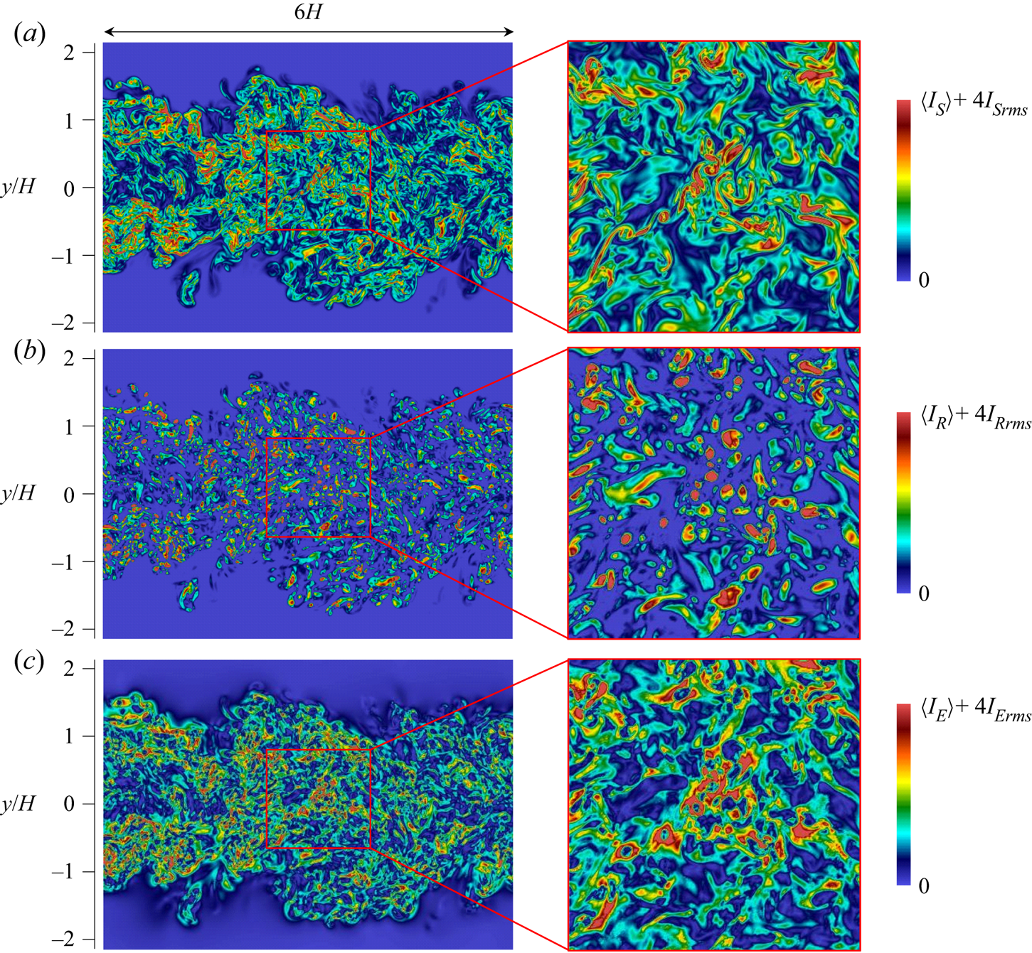
Figure 7. Colour contour plots of (a)  $I_S$, (b) $I_R$ and (c) $I_E$ on an $x$–
$x$– $y$ plane in the planar jet with $Re_J=10\,000$ ( $t=20t_r$). The maximum value of colour contour $\langle I_\alpha \rangle +4I_{\alpha rms}$ ( $\alpha =S,R$ or $E$) is determined with the statistics at $y=0$.
Figure 8 visualizes isosurfaces of  $I_S=\langle I_S \rangle +4I_{S rms}$ in the planar jet with $Re_J=10\,000$, where the isosurface value is determined by $\langle I_S\rangle$ and $I_{S rms}$ at $y=0$. A large number of thin sheetlike structures are visualized with $I_S$, which detects well the shear layers in the turbulent planar jet. Similar structures were also identified with $I_S$ in homogeneous isotropic turbulence (Watanabe et al. Reference Watanabe, Tanaka and Nagata2020). The flow field around the shear layers is investigated with the averages taken in the shear coordinate in § 4.3.

Figure 8. (a) Visualization of isosurfaces of  $I_S=I_{Sth}$ in the planar jet with $Re_J=10\,000$ ( $t=20t_r$), where $I_{Sth}=\langle I_S\rangle +4I_{Srms}$ is calculated with $\langle I_S\rangle$ and $I_{Srms}$ at $y=0$. (b) Close-up of one of the isosurfaces in (a).
4.2. Statistics of tensors of shear, rotation and elongation
Figure 9 shows the lateral profiles of averages of the intensities of three motions,  $\langle I_S\rangle$, $\langle I_R\rangle$ and $\langle I_E\rangle$, in the planar jet with $Re_J=10\,000$. The averaged intensities weakly depend on $y$ for $|y/b_u|\lesssim 0.8$, and decrease with $|y|$ for $|y/b_u|\gtrsim 0.8$ because the flow outside the jet has small velocity gradients. For $|y/b_u|\lesssim 2$, $\langle I_S\rangle$ is the largest among three motions, and the turbulent jet is dominated by shearing motion. The intermittency factor in figure 4(a) indicates that the turbulent region of the jet hardly reaches $|y/b_u|\gtrsim 2.5$, where $\langle I_E\rangle$ is larger than $\langle I_S\rangle$ and $\langle I_R\rangle$. It is known that the velocity gradient is not negligible outside a turbulent jet because of velocity fluctuations induced by the jet (da Silva & Pereira Reference da Silva and Pereira2008). Figure 9 further confirms that the induced velocity fluctuations are associated with elongation $\boldsymbol {\nabla } {\boldsymbol {u}}_E$ rather than rotation and shear, which seem to be important only inside the turbulent jet region.
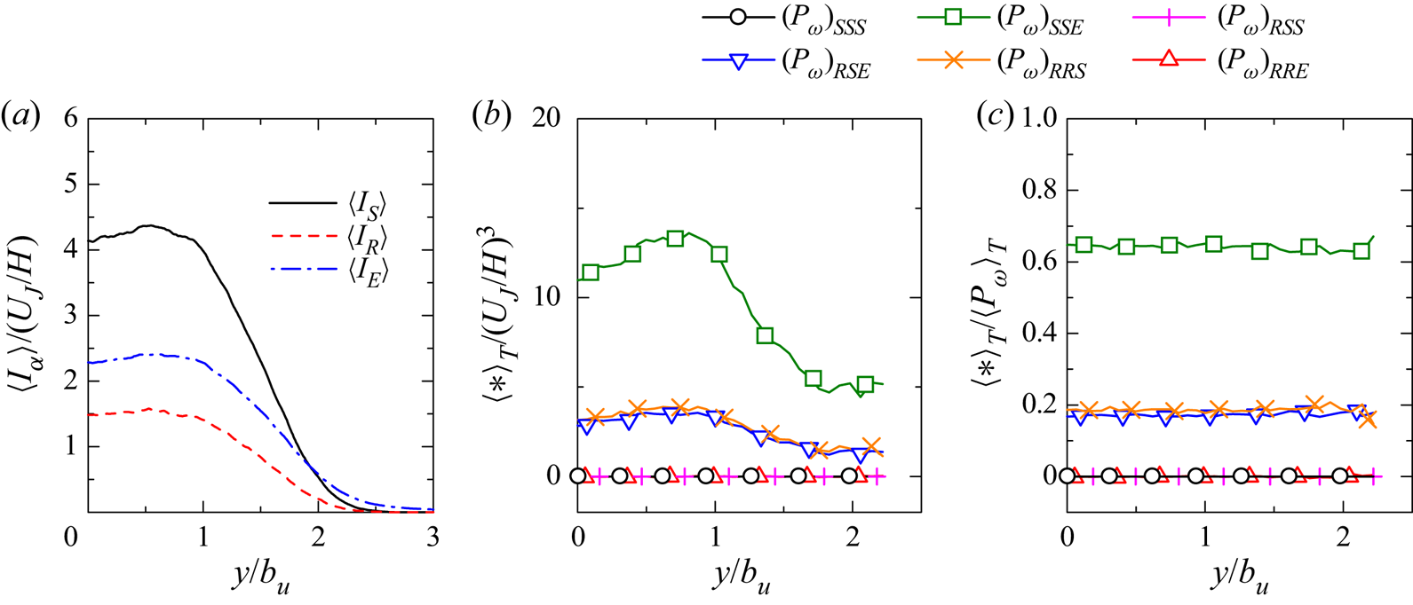
Figure 9. (a) Lateral profiles of mean values of  $I_S$, $I_R$ and $I_E$. (b) Averages of enstrophy production terms in (4.1). (c) Relative contribution to mean enstrophy production $\langle (P_{\omega })_{\alpha \beta \gamma }\rangle _T/\langle P_{\omega }\rangle _T$. The results are taken from the planar jet with $Re_J=10\,000$ ( $t=20t_r$).
The enstrophy production  $P_{\omega }=\omega _i {\mathsf{S}}_{ij} \omega _j$ can be decomposed with the triple decomposition as (Watanabe et al. Reference Watanabe, Tanaka and Nagata2020)
 \begin{equation} P_{\omega}= (P_{\omega})_{SSS} +(P_{\omega})_{SSE} +(P_{\omega})_{RSS} +(P_{\omega})_{RSE} +(P_{\omega})_{RRS} +(P_{\omega})_{RRE}, \end{equation}
with
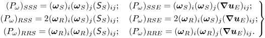 \begin{equation} \left.\begin{gathered}
(P_{\omega})_{SSS}=(\boldsymbol{\omega}_{S})_{i}(\boldsymbol{\omega}_{S})_{j}({\mathsf{S}}_{S})_{ij};\quad
(P_{\omega})_{SSE}=(\boldsymbol{\omega}_{S})_{i}(\boldsymbol{\omega}_{S})_{j}(\boldsymbol{\nabla}
{\boldsymbol{u}}_{E})_{ij};\\
(P_{\omega})_{RSS}=2(\boldsymbol{\omega}_{R})_{i}(\boldsymbol{\omega}_{S})_{j}({\mathsf{S}}_{S})_{ij};\quad
(P_{\omega})_{RSE}=2(\boldsymbol{\omega}_{R})_{i}(\boldsymbol{\omega}_{S})_{j}(\boldsymbol{\nabla}
{\boldsymbol{u}}_{E})_{ij};\\
(P_{\omega})_{RRS}=(\boldsymbol{\omega}_{R})_{i}(\boldsymbol{\omega}_{R})_{j}({\mathsf{S}}_{S})_{ij};\quad
(P_{\omega})_{RRE}
=(\boldsymbol{\omega}_{R})_{i}(\boldsymbol{\omega}_{R})_{j}(
\boldsymbol{\nabla} {\boldsymbol{u}}_{E})_{ij}.
\end{gathered}\right\}
\end{equation}
\begin{equation} \left.\begin{gathered}
(P_{\omega})_{SSS}=(\boldsymbol{\omega}_{S})_{i}(\boldsymbol{\omega}_{S})_{j}({\mathsf{S}}_{S})_{ij};\quad
(P_{\omega})_{SSE}=(\boldsymbol{\omega}_{S})_{i}(\boldsymbol{\omega}_{S})_{j}(\boldsymbol{\nabla}
{\boldsymbol{u}}_{E})_{ij};\\
(P_{\omega})_{RSS}=2(\boldsymbol{\omega}_{R})_{i}(\boldsymbol{\omega}_{S})_{j}({\mathsf{S}}_{S})_{ij};\quad
(P_{\omega})_{RSE}=2(\boldsymbol{\omega}_{R})_{i}(\boldsymbol{\omega}_{S})_{j}(\boldsymbol{\nabla}
{\boldsymbol{u}}_{E})_{ij};\\
(P_{\omega})_{RRS}=(\boldsymbol{\omega}_{R})_{i}(\boldsymbol{\omega}_{R})_{j}({\mathsf{S}}_{S})_{ij};\quad
(P_{\omega})_{RRE}
=(\boldsymbol{\omega}_{R})_{i}(\boldsymbol{\omega}_{R})_{j}(
\boldsymbol{\nabla} {\boldsymbol{u}}_{E})_{ij}.
\end{gathered}\right\}
\end{equation}
Here,  $({\mathsf{S}}_{S})_{ij}=[(\boldsymbol {\nabla }{\boldsymbol {u}}_{S})_{ij}+(\boldsymbol {\nabla } {\boldsymbol {u}}_{S})_{ji}]/2$ is a symmetric part of the shear tensor and $({\boldsymbol {\omega }}_{S})_{i}= \epsilon _{ijk}(\boldsymbol {\nabla } {\boldsymbol {u}}_{S})_{jk}$ and $({\boldsymbol {\omega }}_{R})_{i}= \epsilon _{ijk}(\boldsymbol {\nabla } {\boldsymbol {u}}_{R})_{jk}$ are the vorticity vectors of $\boldsymbol {\nabla } {\boldsymbol {u}}_{S}$ and $\boldsymbol {\nabla } {\boldsymbol {u}}_{R}$, respectively. The decomposed terms represent the interactions of three motions considered in the triple decomposition. Figure 9(b) shows the averages of these decomposed terms, where the averages are taken in the turbulent region as $\langle (P_{\omega })_{\alpha \beta \gamma }\rangle _T$. The interaction between motions of shear and elongation, $\langle (P_{\omega })_{SSE}\rangle _T$, has a dominant contribution to the mean enstrophy production while $\langle (P_{\omega })_{RSE}\rangle _T$ and $\langle (P_{\omega })_{RRS}\rangle _T$ also have positive values. These terms involve the interactions of shearing motion with other motions. The enstrophy production is large near the centreline and decreases in the intermittent region ( $y/b_u\gtrsim 1$). The relative contributions to the mean enstrophy production are evaluated by $\langle (P_{\omega })_{\alpha \beta \gamma }\rangle _T/\langle P_{\omega }\rangle _T$. In the turbulent planar jet, $\langle (P_{\omega })_{SSE}\rangle _T/\langle P_{\omega }\rangle _T\approx 0.65$, $\langle (P_{\omega })_{RSE}\rangle _T/\langle P_{\omega }\rangle _T\approx 0.17$ and $\langle (P_{\omega })_{RRS}\rangle _T/\langle P_{\omega }\rangle _T\approx 0.19$ hardly vary in the $y$ direction. In homogeneous isotropic turbulence, $\langle (P_{\omega })_{SSE}\rangle /\langle P_{\omega }\rangle \approx 0.69$, $\langle (P_{\omega })_{RSE}\rangle /\langle P_{\omega }\rangle \approx 0.17$ and $\langle (P_{\omega })_{RRS}\rangle /\langle P_{\omega }\rangle \approx 0.18$ were obtained for $Re_\lambda =43\text {--}296$ (Watanabe et al. Reference Watanabe, Tanaka and Nagata2020). Thus, the relative contributions of the decomposed production terms are similar for the planar jet and homogeneous isotropic turbulence, and the physical mechanism of the enstrophy production is the same for these flows.
Figure 10(a,b) shows probability density functions (p.d.f.s) of  $I_S$, $I_R$ and $I_E$ at $y=0$ and $1.2b_u$ in the planar jet with $Re_J=10\,000$. Figure 10(c) shows the p.d.f.s obtained with the DNS database of statistically stationary, homogeneous isotropic turbulence with $Re_{\lambda }=72$ (Watanabe et al. Reference Watanabe, Tanaka and Nagata2020). The p.d.f.s are similar between the centre of the turbulent jet and isotropic turbulence. The p.d.f. of $I_R$ has a large peak at $I_R=0$, and the motion of rotation is mostly negligible and appears intermittently in space. This is also confirmed in figure 7(b), where regions with $I_R>0$ occupy a small part of the flow. On the other hand, the p.d.f. of $I_S$ and $I_E$ has a peak for $I_S>0$ and $I_E>0$, and the turbulent jet has moderately strong motions of shear and elongation in most of the flow. In figure 10(b), the p.d.f. at $y=1.2b_u$ has a peak at $I_S=0$. Turbulent and non-turbulent regions intermittently exist at this location. Therefore, the peak of p.d.f. at $I_S=0$ is caused by the existence of non-turbulent fluid where shearing motion is absent. However, the p.d.f. at $I_E=0$ is still low even at $y=1.2b_u$, indicating that the non-turbulent fluid near the jet also has moderately strong motion of elongation. For the same reason, $\langle I_E\rangle$ decreases more slowly with large $y$ than $\langle I_S\rangle$ in figure 9(a).
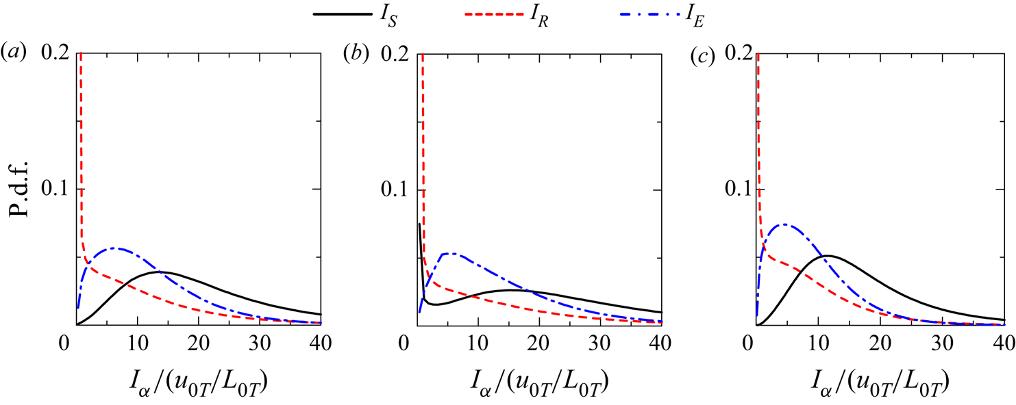
Figure 10. The p.d.f.s of  $I_S$, $I_R$ and $I_E$ at (a) $y=0$ and (b) $y=1.2b_u$ of the planar jet with $Re_J=10\,000$ ( $t=20t_r$). (c) The p.d.f.s of $I_S$, $I_R$ and $I_E$ in homogeneous isotropic turbulence with $Re_{\lambda }=72$ taken from DNS used in Watanabe et al. (Reference Watanabe, Tanaka and Nagata2020).
4.3. Mean flow characteristics around shear layers
Mean flow patterns around the shear layers are studied with ensemble averages taken for local maxima of  $I_S$ with (3.9)–(3.14). Figure 11 shows two-dimensional profiles of the mean velocity vector $(\overline {u_1},\overline {u_2},\overline {u_3})$ and a colour contour of the mean shear intensity $\overline {I_S}$ obtained at $y=0$. Here, figures 11(a) and 11(b) visualize the $\zeta _2$– $\zeta _3$ plane at $\zeta _1=0$ and the $\zeta _1$– $\zeta _2$ plane at $\zeta _3=0$, respectively. A region with large $\overline {I_S}$ has a flattened shape, which is expanded in the $\zeta _1$ and $\zeta _3$ directions. The thickness of the region with large $\overline {I_S}$ is about $5\eta _T$ in the $\zeta _2$ direction while its spatial extent in the $\zeta _1$ and $\zeta _3$ directions is about $20\eta _T$. A shear layer pattern due to the flows in $\pm \zeta _3$ directions can be observed in the velocity vector on the $\zeta _2$– $\zeta _3$ plane in figure 11(a). The mean velocity vector in figure 11(b) exhibits biaxial strain with compression in the $\zeta _2$ direction and stretching in the $\zeta _1$ direction. The $\zeta _1$ direction is taken in the direction of the vorticity of shear $\boldsymbol {\omega }_{S}$, which is effectively amplified by the stretching in the $\zeta _1$ direction. This observation is consistent with figure 9(b,c), where the enstrophy production is dominated by the interaction between motions of shear and elongation. The shear layers in homogeneous isotropic turbulence also cause the enstrophy production by this interaction (Watanabe et al. Reference Watanabe, Tanaka and Nagata2020). Figure 12 presents the results obtained at $y/b_u=1$, where the mean velocity gradient is large as shown in figure 2(a). The mean velocity vector and the profile of $I_S$ are similar at $y/b_u=0$ and $1$. Similar mean flow patterns of the shear and biaxial strain were found for the shear layers in homogeneous isotropic turbulence (Watanabe et al. Reference Watanabe, Tanaka and Nagata2020). Thus, the local flow topology associated with shearing motion is not qualitatively influenced by the mean velocity gradient of the planar jet.
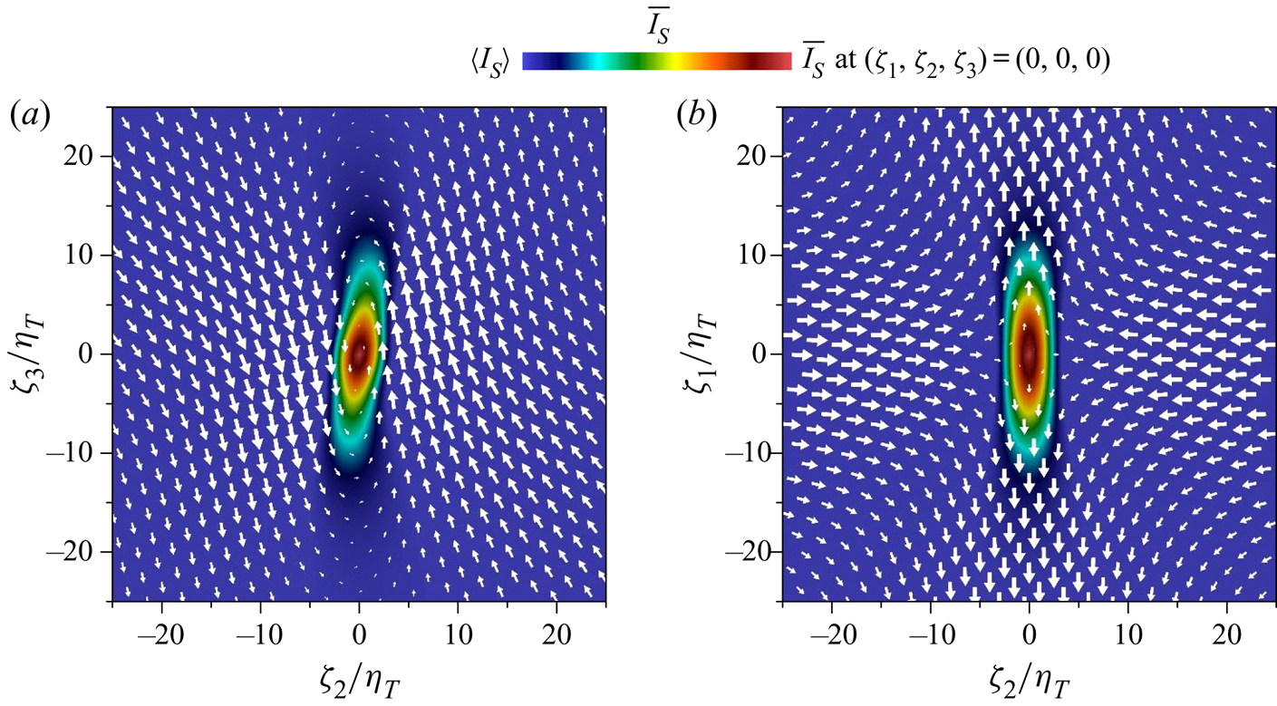
Figure 11. Mean velocity vector and colour contour of  $\overline {I_S}$ on (a) $\zeta _2$– $\zeta _3$ plane at $\zeta _1=0$ and (b) $\zeta _1$– $\zeta _2$ plane at $\zeta _3=0$. The length of the vectors represents the magnitude of the velocity vector on each plane. The results are taken at $y=0$ of the planar jet with $Re_J=10\,000$.

Figure 12. Mean velocity vector and  $\overline {I_S}$ of the shear layers at $y/b_u=1$ ( $Re_J=10\,000$) on (a) $\zeta _2$– $\zeta _3$ plane at $\zeta _1=0$ and (b) $\zeta _1$– $\zeta _2$ plane at $\zeta _3=0$.
Figure 13 shows the mean velocity profile along the  $\zeta _1$ and $\zeta _2$ axes, where $\overline {u_1}$ on the $\zeta _1$ axis and $\overline {u_2}$ and $\overline {u_3}$ on the $\zeta _2$ axis significantly change near the centre of the shear layer. These velocity components are associated with the shear and biaxial strain and have large positive and negative peaks. The shear layer formed in the region of biaxial strain is consistent with the Burgers vortex layer, which is one of the exact solutions of Navier–Stokes equations (Davidson Reference Davidson2004). The Burgers vortex layer has a velocity profile given by
 \begin{equation} u_{1}=\alpha \zeta_1,\quad u_{2}={-}\alpha \zeta_2,\quad u_{3}=\Delta u_{3} \mathrm{erf}(\zeta_2/\delta), \end{equation}
where  $\delta$ is the thickness of the layer and $\Delta u_{3}$ is the velocity jump, which is related to the shear intensity by $I_{S}=\sqrt {2 (\partial u_{3}/\partial \zeta _{2})^{2}}$. A parameter $\alpha$ represents the intensity of the biaxial strain acting on the Burgers vortex layer, where $I_E$ of the triple decomposition is related to $\alpha$ by $\alpha =I_E/2$. The velocity profile around $(\zeta _1, \zeta _2, \zeta _3)=(0,0,0)$ in the planar jet is consistent with the Burgers vortex layer as confirmed from $\partial u_{1}/ \partial \zeta _1>0$, $\partial u_{2}/ \partial \zeta _2<0$ and $\partial u_{3}/ \partial \zeta _2>0$ at $(\zeta _1, \zeta _2, \zeta _3)=(0,0,0)$ in figure 13. In a steady state, the thickness $\delta$ of the Burgers vortex layer is determined by $\alpha$ and $\nu$ as $\delta =\sqrt {2\nu /\alpha }$. If the biaxial strain were absent, the layer thickness would grow with time because of viscous diffusion (Davidson Reference Davidson2004). Therefore, compression due to the biaxial strain keeps the shear layer thin in the Burgers vortex layer. Figure 11 suggests that the thinning effect by the biaxial strain also exists for the shear layers in the planar jet, where the compression in the $\zeta _2$ direction is caused by the biaxial strain. One of the apparent differences between the shear layers in the planar jet and the Burgers vortex layer is the spatial extent in the $\zeta _1$ and $\zeta _3$ directions. The region with large $\overline {I_{S}}$ appears for $|\zeta _1|\lesssim 10\eta _T$ and $|\zeta _3|\lesssim 10\eta _T$ in figure 11 while the Burgers vortex layer has an infinite length in the $\zeta _1$ and $\zeta _3$ directions. Visualization of the shear layers in figure 8(b) also suggests that the size of the shear layer in these directions is of the order of 10 times the Kolmogorov length scale.
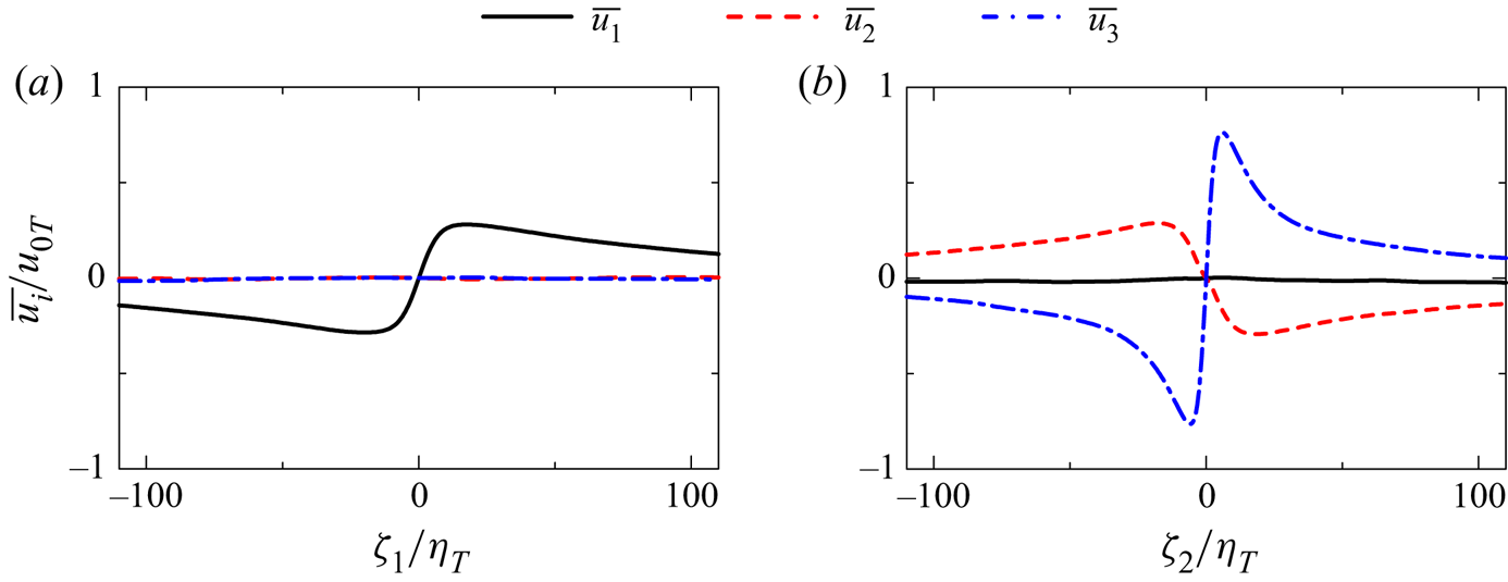
Figure 13. Mean velocity profiles around local maxima of  $I_S$ on (a) $\zeta _1$ axis and (b) $\zeta _2$ axis. The results are taken on the centreline of the planar jet with $Re_J=10\,000$.
4.4. Reynolds number dependence of shear layers
The mean velocity jump around the centre of the shear layer is found for  $\overline {u_1}$ on the $\zeta _1$ axis and $\overline {u_2}$ and $\overline {u_3}$ on the $\zeta _2$ axis in figure 13. The velocity jump $\Delta u_i$ is quantified with local maximum and minimum of these mean velocity components as shown in figure 14, where an example of $\overline {u_i}$ is shown on the $\zeta _\alpha$ axis. The width $\delta _i$ of the velocity jump $\Delta u_i$ is estimated with the mean velocity gradient in the shear layer $\partial \overline {u_i}/\partial \zeta _\alpha$ at $\zeta_\alpha=0$ as $\delta _i = \Delta u_i/|\partial \overline {u_i}/\partial \zeta _\alpha |$, where $\alpha =1$ for $\overline {u_1}$ and $\alpha =2$ for $\overline {u_2}$ and $\overline {u_3}$ are considered. Width $\delta _i$ is defined for the small-scale shear layers, where local shear arises from velocity fluctuations, and this length is expected to be smaller than the length scale that characterizes the mean shear (Thiesset et al. Reference Thiesset, Schaeffer, Djenidi and Antonia2014). Reynolds number dependence of $\Delta u_i$ and $\delta _i$ on the jet centreline is examined in this subsection in comparison with DNS results of homogeneous isotropic turbulence (Watanabe et al. Reference Watanabe, Tanaka and Nagata2020). The dependence on the lateral position in the planar jet is addressed in the next subsection.
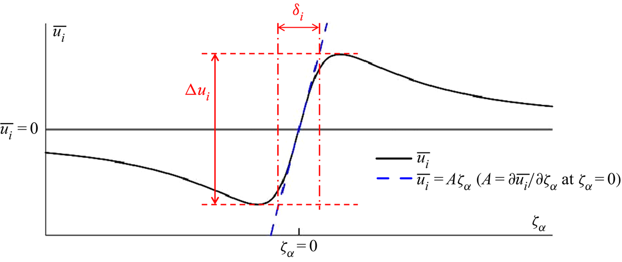
Figure 14. Definitions of the velocity jump  $\Delta u_i$ and its width $\delta _i$ of a mean velocity profile around shear layers.
Figure 15 shows the mean velocity jumps  $\Delta u_i$ normalized by the Kolmogorov velocity scale $u_{\eta }$ or the characteristic velocity scale of large-scale motions $u_0$ as functions of the turbulent Reynolds number $Re_\lambda$. Here $\Delta u_i/u_{\eta }$ hardly depends on $Re_\lambda$ while $\Delta u_i/u_{0}$ decreases with $Re_\lambda$. Both homogeneous isotropic turbulence and the planar jet have $\Delta u_1/u_{\eta }\approx \Delta u_2/u_{\eta }\approx 3$. These velocity components are associated with the biaxial strain acting on the shear layer. The value of $\Delta u_3/u_{\eta }$ is slightly larger in the planar jet than in the homogeneous isotropic turbulence although this difference is small: $\Delta u_3/u_{\eta }\approx 7.8$ in the jet and $\Delta u_3/u_{\eta }\approx 6.2$ in the homogeneous isotropic turbulence. Therefore, the velocity jumps around the shear layers scale with the Kolmogorov velocity scale in the planar jet and homogeneous isotropic turbulence. The broken lines in figure 15(b) represent a power law $\Delta u_i/u_{0}\sim Re_{\lambda }^{a_i}$ with the exponent $a_i$ obtained with a least square method applied for the data of the planar jet. The ratio between $u_{0}$ and $u_{\eta }$ varies with a power law of $Re_{\lambda }$ as $u_{\eta }/u_{0}\sim Re_{\lambda }^{-0.5}$ in isotropic turbulence (Pope Reference Pope2000), and constant $\Delta u_i/u_{\eta }$ implies $\Delta u_i/u_{0}\sim Re_{\lambda }^{-0.5}$. The present DNS data of the planar jet yield $a_1=-0.45$, $a_2=-0.46$ and $a_3=-0.49$, which are close to the exponent $-0.5$ predicted from constant $\Delta u_i/u_{\eta }$. However, $a_1$ and $a_2$ are slightly smaller than $-0.5$, and $\Delta u_2/u_\eta$ and $\Delta u_3/u_\eta$ gradually increase with $Re_\lambda$.
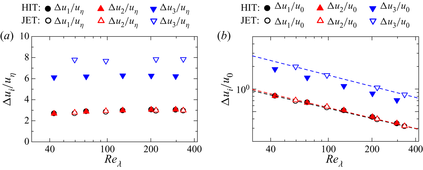
Figure 15. The  $Re_\lambda$ dependence of the mean velocity jumps around shear layers: (a) $\Delta u_i$ normalized by the Kolmogorov velocity scale $u_\eta$; (b) $\Delta u_i$ normalized by the velocity scale of large-scale motions $u_0$. The results at the centre ( $y=0$) of the planar jets (JET) are compared with DNS results of homogeneous isotropic turbulence (HIT) (Watanabe et al. Reference Watanabe, Tanaka and Nagata2020). The broken lines in (b) represent power laws obtained with a least square method applied to the jet data.
Figure 16 compares the  $Re_\lambda$ dependence of $\delta _i$ between the planar jet and homogeneous isotropic turbulence, where $\delta _i$ is normalized by the Kolmogorov length scale $\eta$ in figure 16(a) and by the integral scale $L_{0}$ in figure 16(b). In both panels, the difference between the planar jet and homogeneous isotropic turbulence is small, and the normalized length scales of the shear layer hardly depend on the flows. As also found for $\Delta u_3$, $\delta _3/\eta$ hardly varies with Reynolds number. In the planar jet, $\delta _3/\eta =6$ is obtained by averaging the results of all Reynolds numbers examined in this study. On the other hand, $\delta _1/\eta$ and $\delta _2/\eta$ increase with $Re_\lambda$. However, the $Re_\lambda$ dependence is much smaller for $\delta _1/\eta$ and $\delta _2/\eta$ than for $\delta _1/L_0$ and $\delta _2/L_0$. As $\eta /L_{0}$ varies with $Re_\lambda ^{-1.5}$ in isotropic turbulence (Pope Reference Pope2000), we expect a power law of $\delta _i/L_0\sim Re_\lambda ^{-1.5}$ when $\delta _i/\eta$ is constant. Figure 16(b) shows $\delta _i/L_0$ with a power law $\delta _i/L_0\sim Re_\lambda ^{b_i}$ obtained with a least square method applied to the jet data. The present DNS results yield $b_1=-1.36$, $b_2=-1.37$ and $b_3=-1.44$, which are close to $-1.5$ expected from constant $\delta _i/\eta$. Therefore, the shear layers are small-scale structures whose length scales are characterized by the Kolmogorov length scale.

Figure 16. The  $Re_\lambda$ dependence of the characteristic length scales $\delta _i$ of shear layers: (a) $\delta _i$ normalized by the Kolmogorov length scale $\eta$; (b) $\delta _i$ normalized by the integral scale $L_0$. The results at the centre ( $y=0$) of the planar jets (JET) are compared with DNS results of homogeneous isotropic turbulence (HIT) (Watanabe et al. Reference Watanabe, Tanaka and Nagata2020). The broken lines in (b) represent power laws obtained with a least square method applied to the jet data.
If  $\Delta u_i$ scales with the velocity scale defined with the Taylor microscale, $\nu /\lambda$ (Cafiero & Vassilicos Reference Cafiero and Vassilicos2020), $\Delta u_i$ follows $\Delta u_i/u_{0} \sim Re_{\lambda }^{-1}$. The present DNS yields $\Delta u_i/u_{0} \sim Re_{\lambda }^{a_i}$ with $a_1=-0.45$, $a_2=-0.46$ and $a_3=-0.49$, which are closer to the exponent of the the Kolmogorov scaling $-0.5$ than $-1$. The scaling for $\delta _i$ with the Taylor microscale requires $\delta _i/L_0\sim Re_\lambda ^{-1}$ while figure 16 yields $\delta _i/L_0\sim Re_\lambda ^{b_i}$ with $b_1=-1.36$, $b_2=-1.37$ and $b_3=-1.44$. These exponents are also closer to that of the Kolmogorov scaling $-1.5$ than $-1$. Thus, the length and velocity of the shear layers better scale with the Kolmogorov scale than the Taylor microscale. The differences of $b_i$ from $-1.5$ are slightly larger for $i=1$ and 2 than 3. Therefore, $\delta _1/\eta$ and $\delta _2/\eta$ increase with $Re_{\lambda }$ in figure 16(a) and the size of the shear layers in these directions is not determined solely by $\eta$. This tendency is observed in both planar jet and homogeneous isotropic turbulence.
Figure 17 shows the number density  $N_{SH}$ of local maxima of $I_S$ used in the shear layer analysis. Parameter $N_{SH}$ is calculated as the number of the local maxima of $I_S$ divided by the volume of the turbulent region $V_T$. If the turbulent region is filled by the shear layers whose size varies with $\delta _i\sim L_{0}Re_{\lambda }^{-1.4}$, we may estimate that $N_{SH}$ increases with $(Re_{\lambda }^{-1.4})^{-3}=Re_{\lambda }^{4.2}$. In figure 17, $N_{SH}$ increases with $Re_{\lambda }$. A least square method yields $N_{SH}\sim Re_{\lambda }^{3.9}$, which is not far from the above estimation. Here, the results shown in the figure do not consider the spatial variation of $Re_{\lambda }$ as $Re_{\lambda }$ is taken from the jet centreline. At least, the present shear layer detection method yields the $Re_{\lambda }$ dependence of $N_{SH}$ close to the estimation based on $\delta _i\sim L_{0}Re_{\lambda }^{-1.4}$.
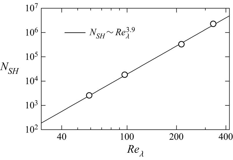
Figure 17. The number density  $N_{SH}$ of local maxima of $I_S$ used in the shear layer analysis. Here $N_{SH}$ calculated in the entire turbulent region of the jet is plotted against $Re_{\lambda }$ on the jet centreline.
The mean intensities of the shear and biaxial strain of the shear layers are evaluated as  $\overline {I_S}$ and $\overline {I_E}$ at $(\zeta _1,\zeta _2,\zeta _3)=(0,0,0)$. Figure 18(a) presents $\overline {I_S}$ and $\overline {I_E}$ normalized by $(u_{0}/L_{0})$ as functions of the turbulent Reynolds number. The normalized shear and strain intensities agree well between the planar jet and homogeneous isotropic turbulence, and follow a power law of $Re_{\lambda }$. The power law exponents obtained by a least square method are $0.94$ for $\overline {I_S}/(u_{0}/L_{0})$ and $0.93$ for $\overline {I_E}/(u_{0}/L_{0})$ for the planar jet. Because of $(u_{0}/L_{0})\sim (u_{\eta }/\eta )Re_{\lambda }^{-1}$, the power exponents close to $1$ suggest that $\overline {I_S}/(u_{\eta }/\eta )$ and $\overline {I_E}/(u_{\eta }/\eta )$ hardly depend on $Re_{\lambda }$ in these flows.

Figure 18. The  $Re_\lambda$ dependence of (a) mean intensities of shear $\overline {I_{S}}$ and elongation $\overline {I_{E}}$ at $(\zeta _1,\zeta _2,\zeta _3)=(0,0,0)$ normalized by $u_0/L_0$ and (b) shear Reynolds number $Re_S$. The results at the centre ( $y=0$) of the planar jets (JET) are compared with DNS results of homogeneous isotropic turbulence (HIT) (Watanabe et al. Reference Watanabe, Tanaka and Nagata2020). The broken lines in (a) represent power laws obtained with a least square method applied to the jet data.
The Reynolds number of the shear layer can be defined as  $Re_S=\Delta u_3 \delta _3/\nu$, which is based on the velocity jump of the shear and the layer thickness. Figure 18(b) plots $Re_S$ against the turbulent Reynolds number in the planar jet and homogeneous isotropic turbulence. Although $Re_S$ in each flow slowly increases with $Re_{\lambda }$, we obtain $Re_S\approx 45$ in the jet and $Re_S\approx 30$ in the homogeneous isotropic turbulence for a wide range of $Re_{\lambda }$. Weak $Re_\lambda$ dependence of $Re_S$ is expected from the scaling of $\Delta u_3$ and $\delta _3$. With the definitions of $Re_S$, $\eta$ and $u_\eta$, $Re_S$ can be rewritten as $Re_S=(\Delta u_3/u_\eta )(\delta _3/\eta )$. Therefore, $Re_S$ does not depend on $Re_{\lambda }$ when $\Delta u_3/u_\eta$ and $\delta _3/\eta$ are constant. Reynolds number $Re_S$ is slightly larger in the planar jet than in homogeneous isotropic turbulence because $\Delta u_3/u_\eta$ is also larger in the jet. It is important to note that both flows have $Re_S\sim {{O}}(10^{1})$, which is high enough for the shear layers to become unstable (Beronov & Kida Reference Beronov and Kida1996), and the instability of the shear layers can result in the formation of vortex tubes in these flows.
The thickness of each shear layer can be estimated with the profile of  $I_S$ obtained for each local maximum of $I_S$. An instantaneous profile $I_S$ on the $\zeta _2$ axis has a peak at $\zeta _2=0$, and rapidly decreases as $|\zeta _2|$ becomes large. Therefore, the thickness of the shear layer $\delta _S$ is evaluated as the half-width of $I_S$ on $\zeta _2$. Namely, $\delta _S$ is the distance between two points on the $\zeta _2$ axis with $I_S=I_{S,max}/2$ for $\zeta _2 >0$ and $\zeta _2 <0$, where $I_{S,max}$ is the value of $I_S$ at $\zeta _2=0$. Figure 19(a) shows the p.d.f. of $\delta _S$ normalized by $\eta$ obtained at $y=0$. The p.d.f. for all Reynolds numbers has a peak at $\delta _S/\eta =5$– $6$. The instability of shear layers generates roller vortices, whose diameter is close to the shear layer thickness. The typical diameter of small-scale vortex tubes in a turbulent planar jet is about $7\eta$ (da Silva et al. Reference da Silva, Dos Reis and Pereira2011), which is close to the typical shear layer thickness $5\eta$– $6\eta$ observed in the present DNS. This result also indicates that small-scale vortex tubes are produced by the instability of shear layers. In the Burgers vortex layer given by (4.3a–c), the half-width of $I_S$ is written with $\nu$ and $I_{E}$ as $\delta _{BV}=1.67\sqrt {4\nu /I_E}$. The thickness of shear layers in the DNS is compared with the prediction by the Burgers vortex layer. Here, for each local maxima of $I_S$, $\delta _{BV}$ is calculated with $I_E$ at $(\zeta _1, \zeta _2, \zeta _3)=(0,0,0)$ while the actual half-width $\delta _S$ is also calculated from the profile of $I_S$ on the $\zeta _2$ axis. Figure 19(b) shows the p.d.f. of $\delta _S/\delta _{BV}$ obtained at $y=0$. A large peak appears at $\delta _S/\delta _{BV}\approx 1$ for all Reynolds numbers. Thus, the shear layer thickness in the planar jet is well predicted by the Burgers vortex layer, which yields the thickness as a function of the intensity of the biaxial strain $I_E$ and kinematic viscosity $\nu$ of the flow.
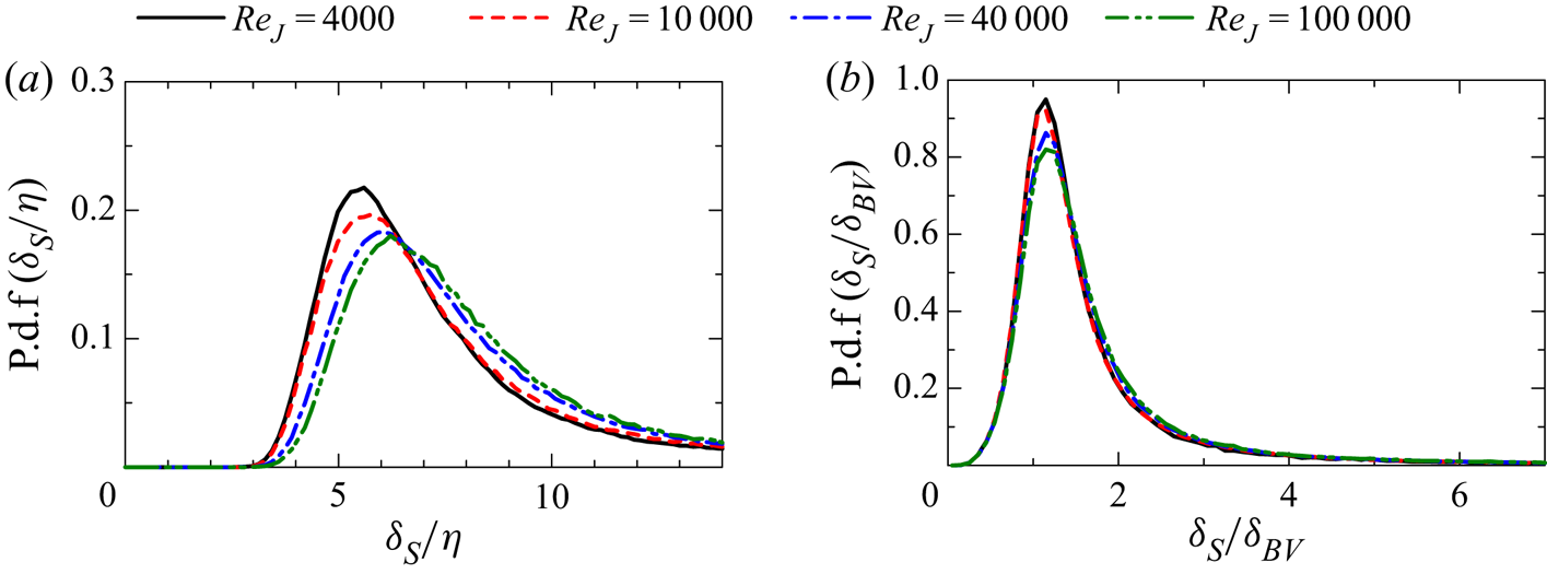
Figure 19. The p.d.f.s of shear layer thickness normalized by (a) Kolmogorov length scale  $\eta$ and (b) Burgers vortex layer thickness $\delta _{BV}$ at $y=0$.
4.5. Shear layers at different lateral positions in the jet
The characteristics of shear layers are examined as functions of the lateral position of the planar jet. Here, the quantities related to the shear layers are normalized by the statistics calculated in the turbulent region with  $\langle \ \rangle _T$. Figure 20(a) shows the velocity jumps $\Delta u_i$ normalized by $u_{\eta T}$ as functions of $y/b_u$. The lateral profiles are similar for all Reynolds numbers. The planar jet has $\Delta u_1\approx \Delta u_2\approx 3u_{\eta T}$ and $\Delta u_3\approx 8u_{\eta T}$, which weakly depend on $y$. Therefore, the velocity jumps of the shear layer at different lateral positions scale with the Kolmogorov velocity scale. Figure 20(b) plots the length scales of the shear layer $\delta _i$ normalized by $\eta _T$. The shear layer thickness $\delta _3$ hardly depends on $y$ when it is normalized by $\eta _T$, and the thickness is about $6\eta _T$ in the planar jet. On the other hand, variations of $\delta _1$ and $\delta _2$ across the jet are more noticeable than variations of $\delta _3$. The centre of the jet has $13\lesssim \delta _1/\eta _T\lesssim 16$ and $25\lesssim \delta _2/\eta _T\lesssim 33$ depending on the Reynolds number. It is evident that $\delta _1/\eta _T$ and $\delta _2/\eta _T$ vary with $y$ as much as with $Re_J$ at $y=0$. These variations are considered small because $\eta _T/H$ used for the normalization changes between ${{O}}(10^{-3})$ and ${{O}}(10^{-4})$ depending on the Reynolds number, and the order of magnitude of $\delta _1/\eta _T$ and $\delta _2/\eta _T$ does not vary with $y$ for all Reynolds numbers. Length scales $\delta _1$ and $\delta _2$ are related to a spatial extent of the region of the biaxial strain. In figure 20(b), the spatial variations of $\delta _1/\eta _T$ and $\delta _2/\eta _T$ with $y$ occur over a distance of the order of $b_u$, which is one of the characteristic length scales of large-scale motions of the jet. Therefore, the profiles of $\delta _1/\eta _T$ and $\delta _2/\eta _T$ imply the possible influence of large-scale fluctuations on the biaxial strain acting on the small-scale shear layers.
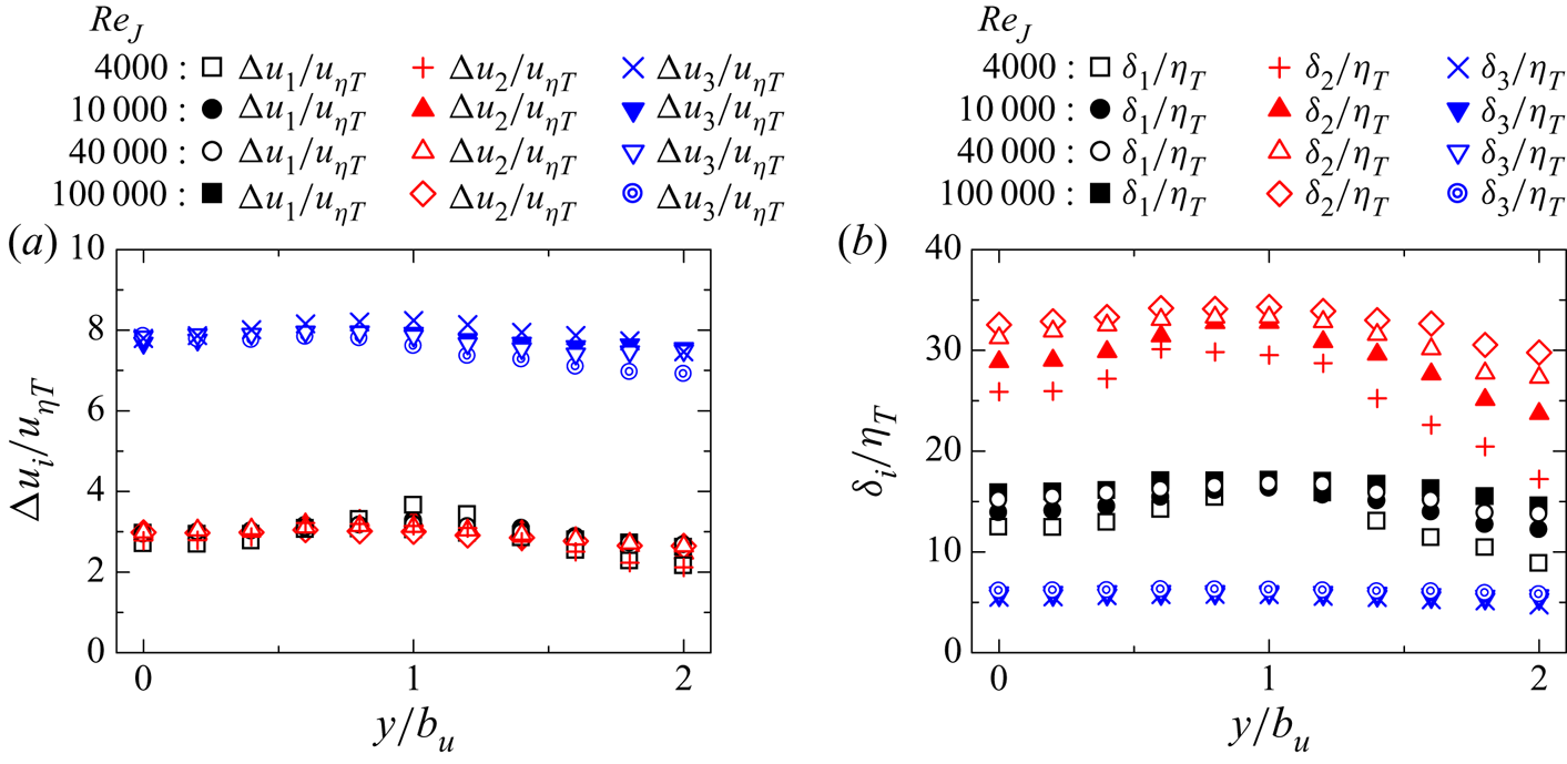
Figure 20. Lateral profiles of (a)  $\Delta u_i/u_{\eta T}$ and (b) $\delta _i/\eta _T$ in the planar jet.
Figure 21 shows the mean intensities of shear and elongation  $\overline {I_S}$ and $\overline {I_E}$ and the shear Reynolds number $Re_S$, where $\overline {I_S}$ and $\overline {I_E}$ are evaluated at $(\zeta _1, \zeta _2, \zeta _3)=(0,0,0)$ and normalized by $(u_{\eta T}/\eta _T)$. These quantities hardly vary in the $y$ direction. Therefore, the intensities of the shear and biaxial strain scale with the Kolmogorov scales in the planar jet. Reynolds number $Re_S\approx 40$ is also obtained across the planar jet for all Reynolds numbers examined in this study.
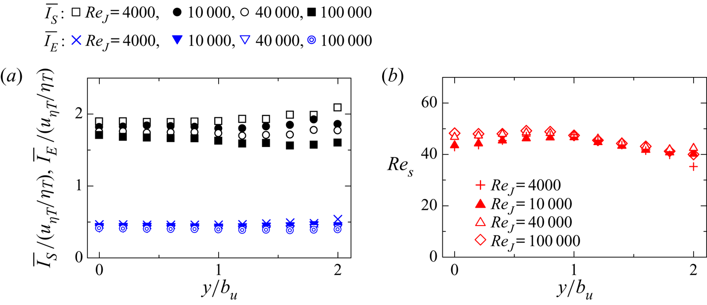
Figure 21. Lateral profiles of (a)  $\overline {I_{S}}/(u_{\eta T}/\eta _T)$ and $\overline {I_{E}}/(u_{\eta T}/\eta _T)$ and (b) $Re_{S}$ in the planar jet.
Figure 22 shows the p.d.f. of  $\delta _S/\eta _T$ and $\delta _S/\delta _{BV}$ obtained at various lateral positions in the planar jet with $Re_{J}=10\,000$. The p.d.f. weakly depends on $y$, and the shear layer thickness normalized by the Kolmogorov length scale hardly changes with $y$. The peak of the p.d.f. in figure 22(a) indicates that the typical thickness of the shear layers is about $6\eta _T$. Furthermore, the p.d.f. of $\delta _S/\delta _{BV}$ peaks at $\delta _S/\delta _{BV}\approx 1$, and the shear layer thickness is well predicted by the Burgers vortex layer in the planar jet.
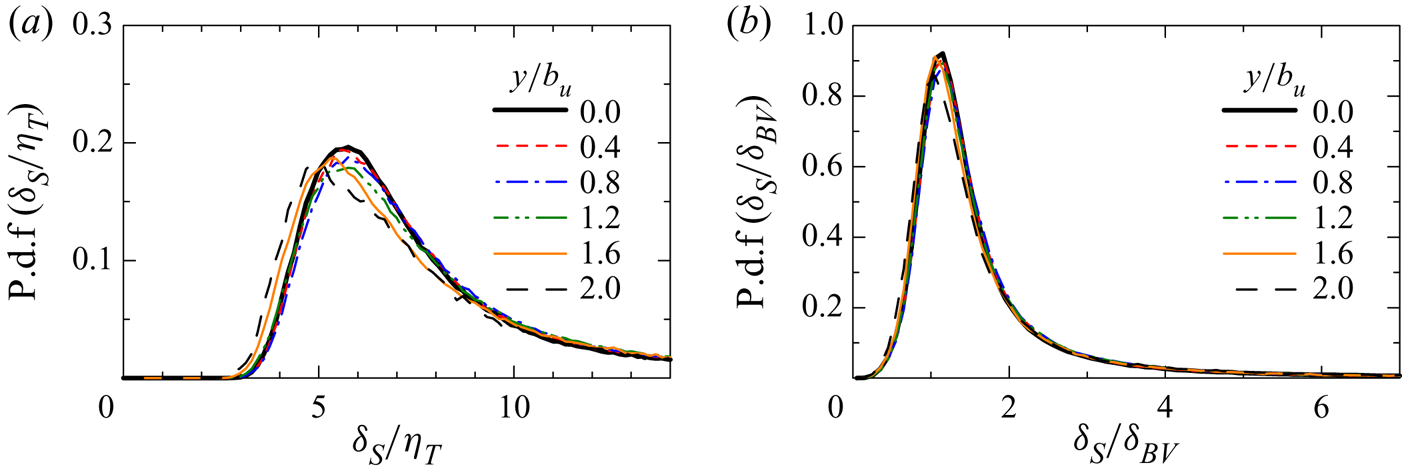
Figure 22. The p.d.f.s of shear layer thickness  $\delta _S$ obtained at different lateral positions of the planar jet with $Re_J=10\,000$. Thickness $\delta _S$ is normalized by (a) Kolmogorov length scale $\eta _T$ and (b) Burgers vortex layer thickness $\delta _{BV}$.
Figure 23(a) shows the lateral profiles of the averages of three components of the shear vorticity,  $\overline {({\boldsymbol {\omega }}_S)_{i}}$, at the centre of the shear layer $(\zeta _1,\zeta _2,\zeta _3)=(0,0,0)$ for $Re_J=10\,000$. In the planar jet, the mean shear $\partial \langle u \rangle /\partial y$ contributes to positive $\overline {({\boldsymbol {\omega }}_S)_{z}}$. Therefore, $\overline {({\boldsymbol {\omega }}_S)_{z}}$ becomes positive away from the jet centreline while $\overline {({\boldsymbol {\omega }}_S)_{x}}$ and $\overline {({\boldsymbol {\omega }}_S)_{y}}$ are close to 0. Figure 23(b) shows the p.d.f. of $({\boldsymbol {\omega }}_S)_{z}$ at the centre of the shear layer detected at $y/b_u=0$ and $1$. Because of the mean shear, the p.d.f. at $y/b_u=1$ is slightly shifted to positive $({\boldsymbol {\omega }}_S)_{z}$. The sign of $({\boldsymbol {\omega }}_S)_{z}$ represents the orientation of the shear in relation to the mean velocity gradient because the spanwise vorticity due to $\partial \langle u \rangle /\partial y$ is positive for $y>0$. If the mean velocity gradient strongly affects the shear within the layer structures, the probability for $({\boldsymbol {\omega }}_S)_{z}>0$ should be much larger than that for $({\boldsymbol {\omega }}_S)_{z}<0$. However, the peak of the p.d.f. appears at $({\boldsymbol {\omega }}_S)_{z}\approx 0$ even at $y/b_u=1$. In a turbulent boundary layer, the local velocity gradient across shear layers often has the same sign as the mean velocity gradient (Eisma et al. Reference Eisma, Westerweel, Ooms and Elsinga2015). It should be noted that they used the two-dimensional triple decomposition, and three-dimensional features of the shear layers are not fully revealed. However, it seems that the mean shear effect on the shear layers is weaker in the turbulent planar jet than in the turbulent boundary layer. It is known that the mean streamwise velocity sharply changes near the interfacial layer between the turbulent and non-turbulent regions (TNTI layer) because the outside of the jet has small $u$ (Westerweel et al. Reference Westerweel, Fukushima, Pedersen and Hunt2009). This mean velocity difference between the turbulent and non-turbulent regions may also affect the sign of $({\boldsymbol {\omega }}_S)_{z}$ in the shear layers. The outer edge of the TNTI layer is well detected as the isosurface $\omega =\omega _{th}$. For the shear layer with the centre location given by $(x_S, y_S, z_S)$, we examine the isosurface location $y_{\omega }$ in the $y$ direction at $(x, z)=(x_S, z_S)$. We only consider the isosurface at $y>y_S$ because the shear layers are analysed for $y>0$. The distance between the shear layer and the isosurface of $\omega =\omega _{th}$ is given by $y_I=y_{\omega }-y_S$, where the isosurface nearest to the shear layer is considered when the $y$ axis crosses the isosurface more than once. The p.d.f. of $({\boldsymbol {\omega }}_S)_{z}$ is calculated for the shear layers located in three regions: $0< y_I/\eta \leqslant 20$, $20< y_I/\eta \leqslant 40$ and $40< y_I/\eta \leqslant 60$. The TNTI layer is formed in $0< y_I/\eta \lesssim 20$ in the temporally evolving planar jet (Silva, Zecchetto & da Silva Reference Silva, Zecchetto and da Silva2018). Figure 23(c) shows the p.d.f. obtained in these regions. The probability for large negative $({\boldsymbol {\omega }}_S)_{z}$ is noticeably small for $0< y_I/\eta \leqslant 20$ compared with the other regions. The mean velocity jump near the TNTI layer contributes to positive $({\boldsymbol {\omega }}_S)_{z}$, and low probability for $({\boldsymbol {\omega }}_S)_{z}<0$ in $0< y_I/\eta \leqslant 20$ can be interpreted as the influence of the mean shear near the TNTI layer. However, the probability for $({\boldsymbol {\omega }}_S)_{z}<0$ is not zero, and the shear layers with the shear orientation opposite to the mean shear also appear even near the TNTI layer.
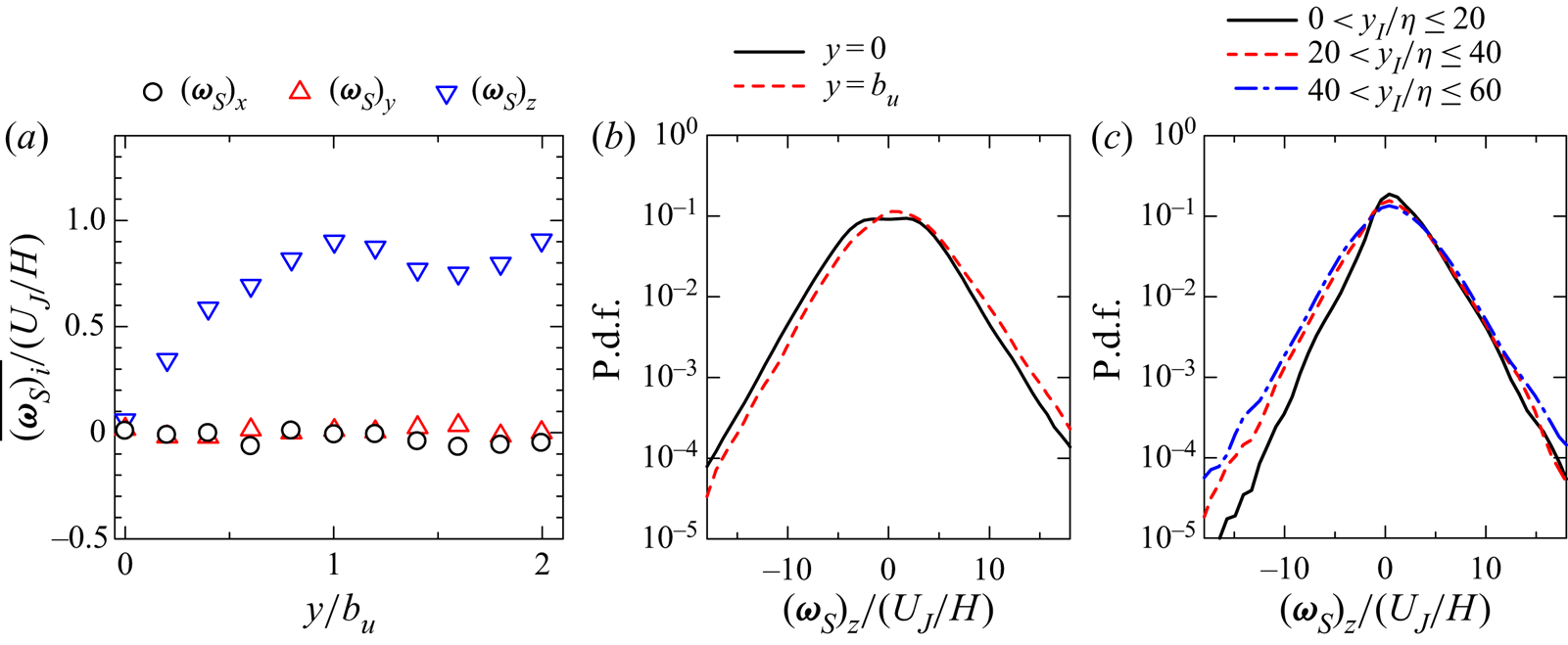
Figure 23. Statistics of shear vorticity  $({\boldsymbol {\omega }}_S)_{i}$ at the centre of the shear layers ( $Re_J=10\,000$). (a) Lateral profiles of the averages of shear vorticity components $\overline {({\boldsymbol {\omega }}_S)_{x}}$, $\overline {({\boldsymbol {\omega }}_S)_{y}}$ and $\overline {({\boldsymbol {\omega }}_S)_{z}}$. (b) The p.d.f. of $({\boldsymbol {\omega }}_S)_{z}$ of the shear layer detected at $y/b_u=0$ and $1$. (c) The p.d.f. of $({\boldsymbol {\omega }}_S)_{z}$ of the shear layers which are located in $0< y_I/\eta \leqslant 20$, $20< y_I/\eta \leqslant 40$ or $40< y_I/\eta \leqslant 60$. Here, $y_I$ is the distance in the $y$ direction from the shear layer to the isosurface of $\omega =\omega _{th}$ and $\eta$ is taken at $y=0$.
5. Conclusion
The characteristics of small-scale shear layers that internally exist in turbulent flows were studied with DNS of temporally evolving turbulent planar jets with Reynolds number  $Re_J=4000$, 10 000, 40 000 and 100 000. The velocity gradient tensor was decomposed into three components that represent motions of shear, rotation and elongation with the triple decomposition (Kolář Reference Kolář2007; Watanabe et al. Reference Watanabe, Tanaka and Nagata2020). In the turbulent planar jet, the shearing motion is stronger than the other motions. However, the motion of elongation becomes dominant far away from the jet centreline. The enstrophy production in the turbulent planar jet is dominated by the interaction between motions of shear and elongation as also found in homogeneous isotropic turbulence (Watanabe et al. Reference Watanabe, Tanaka and Nagata2020). Small-scale shear layers were identified as regions with strong shear. The shear layers were analysed with averages taken around local maxima of the shear intensity $I_S$ in the shear coordinate system, which was defined to express the shear with one component of the shear tensor.
The mean flow pattern around local maxima of  $I_S$ confirmed that a thin shear layer is formed in the region with biaxial strain, which consists of extensive strain in the direction of the vorticity vector of shear and compressive strain in the direction perpendicular to the shear layer. The velocity components associated with the shear and the compression of the biaxial strain rapidly change across the shear layer. Furthermore, the velocity component associated with the extensive strain also rapidly changes within the shear layer in the shear vorticity direction. This extensive strain can cause strong vortex stretching. The velocity jumps across the shear layers scale with the Kolmogorov velocity scale. The shear layer thickness normalized by the Kolmogorov scale also hardly changes with the Reynolds number. Furthermore, the intensities of the shear and biaxial strain of the shear layer also scale with the Kolmogorov scales. These quantities normalized by the Kolmogorov scales only weakly depend on the lateral position of the planar jet when the Kolmogorov scales are defined with averages of turbulent fluids. However, the length scales in the layer-parallel direction, $\delta _1$ and $\delta _2$, normalized by the Kolmogorov scale $\eta _T$ slowly increase with $Re_\lambda$, and their variations across the planar jet are also larger than the shear layer thickness. The large variations of $\delta _1/\eta _T$ and $\delta _2/\eta _T$ imply that the biaxial strain acting on the shear layers is influenced by large-scale velocity fluctuations in the planar jet. The spanwise component of shear vorticity $({\boldsymbol {\omega }}_S)_{z}$ tends to have the same sign as the mean spanwise vorticity when the mean velocity gradient is not zero. A similar effect of the mean velocity gradient was also found within the interfacial layer between the turbulent and non-turbulent regions. However, there also exist a large number of the shear layers with $({\boldsymbol {\omega }}_S)_{z}$ whose sign is opposite to the mean spanwise vorticity. Thus, the mean velocity gradient weakly affects the orientation of the shear layer, and the shear layers are associated with velocity fluctuations rather than the mean velocity gradient of the jet. The characteristics of shear layers normalized by the Kolmogorov scales show good agreement between the planar jet and homogeneous isotropic turbulence, and the small-scale shear layers have some universal properties that are independent of mean velocity gradients and Reynolds numbers.
Funding
The DNS presented in this paper were performed using the high-performance computing system in the Japan Agency for Marine-Earth Science and Technology. This work was also supported by ‘Collaborative Research Project on Computer Science with High-Performance Computing in Nagoya University’ and by JSPS KAKENHI grant no. 20H05754.
Declaration of interests
The authors report no conflict of interest.
Appendix A. Identification of the basic reference frame of the triple decomposition
We use a method proposed in Nagata et al. (Reference Nagata, Watanabe, Nagata and da Silva2020) to identify the basic reference frame, which is chosen from reference frames obtained with three sequential rotational transformations  ${\boldsymbol{\mathsf{Q}}}(\theta _{1},\theta _{2},\theta _{3})$ with angles $\theta _{i}$. The coordinate transformation tensor ${\boldsymbol{\mathsf{Q}}}$ is expressed as
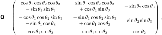 \begin{equation} {\boldsymbol{\mathsf{Q}}} =
\left( \begin{array}{@{}ccc@{}}
{\begin{array}{c}\cos\theta_{1}\cos\theta_{2}\cos\theta_{3}\\ -
\sin\theta_{1}\sin\theta_{3}\end{array}} &
{\begin{array}{c}\sin\theta_{1}\cos\theta_{2}\cos\theta_{3}\\ +
\cos\theta_{1}\sin\theta_{3}\end{array}} &
-\sin\theta_{2}\cos\theta_{3}\\
{\begin{array}{c}-\cos\theta_{1}\cos\theta_{2}\sin\theta_{3}\\ -
\sin\theta_{1}\cos\theta_{3}\end{array}} &
{\begin{array}{c}-\sin\theta_{1}\cos\theta_{2}\sin\theta_{3}\\ +
\cos\theta_{1}\cos\theta_{3}\end{array}} & \sin\theta_{2}\sin\theta_{3}
\\ \cos\theta_{1}\sin\theta_{2} &
\sin\theta_{1}\sin\theta_{2} & \cos\theta_{2}
\end{array}
\right),\end{equation}
\begin{equation} {\boldsymbol{\mathsf{Q}}} =
\left( \begin{array}{@{}ccc@{}}
{\begin{array}{c}\cos\theta_{1}\cos\theta_{2}\cos\theta_{3}\\ -
\sin\theta_{1}\sin\theta_{3}\end{array}} &
{\begin{array}{c}\sin\theta_{1}\cos\theta_{2}\cos\theta_{3}\\ +
\cos\theta_{1}\sin\theta_{3}\end{array}} &
-\sin\theta_{2}\cos\theta_{3}\\
{\begin{array}{c}-\cos\theta_{1}\cos\theta_{2}\sin\theta_{3}\\ -
\sin\theta_{1}\cos\theta_{3}\end{array}} &
{\begin{array}{c}-\sin\theta_{1}\cos\theta_{2}\sin\theta_{3}\\ +
\cos\theta_{1}\cos\theta_{3}\end{array}} & \sin\theta_{2}\sin\theta_{3}
\\ \cos\theta_{1}\sin\theta_{2} &
\sin\theta_{1}\sin\theta_{2} & \cos\theta_{2}
\end{array}
\right),\end{equation}
with the angles in the ranges  $0^{\circ }\leqslant \theta _{1}\leqslant 180^{\circ }$, $0^{\circ }\leqslant \theta _{2}\leqslant 180^{\circ }$ and $0^{\circ }\leqslant \theta _{3}\leqslant 90^{\circ }$. In the basic reference frame, the shear intensity $I_S=\sqrt {2(\boldsymbol {\nabla } {\boldsymbol {u}}_{S})_{ij}(\boldsymbol {\nabla } {\boldsymbol {u}}_{S})_{ij}}$ takes the largest value among all possible reference frames. Hereafter, superscript $*$ represents a tensor evaluated in the rotated reference frame defined with ${\boldsymbol{\mathsf{Q}}}$. For example, the velocity gradient tensor in the rotated frame is calculated as $(\boldsymbol {\nabla } \boldsymbol {u})^{*}=\boldsymbol{\mathsf{Q}}(\boldsymbol {\nabla } \boldsymbol {u} ){\boldsymbol{\mathsf{Q}}^{T}}$. The basic reference frame is identified with the following procedures.
(i) Apply the coordinate transformation (A1) to $\boldsymbol {\nabla } \boldsymbol {u}$ with all sets of $(\theta _{1},\theta _{2},\theta _{3})$ given by
(A2)\begin{gather} \theta_{1}=0, 45^{{\circ}}, 90^{{\circ}}, \dotsc, 180^{{\circ}}, \end{gather}(A3)\begin{gather}\theta_{2}=0, 45^{{\circ}}, 90^{{\circ}}, \dotsc, 180^{{\circ}}, \end{gather}(A4)where the angles are discretely changed by\begin{gather}\theta_{3}=0, 45^{{\circ}}, 90^{{\circ}}, \end{gather}$45^{\circ }$. Calculate $I_S=\sqrt {2(\boldsymbol {\nabla } {\boldsymbol {u}}_{S})^{*}_{ij}(\boldsymbol {\nabla } {\boldsymbol {u}}_{S})^{*}_{ij}}$ in the rotated reference frames with $(\boldsymbol {\nabla } {\boldsymbol {u}}_{S})^{*}_{ij}$ obtained by (3.1).
$\boldsymbol {\nabla } \boldsymbol {u}$ with all sets of $(\theta _{1},\theta _{2},\theta _{3})$ given by
(A2)\begin{gather} \theta_{1}=0, 45^{{\circ}}, 90^{{\circ}}, \dotsc, 180^{{\circ}}, \end{gather}(A3)\begin{gather}\theta_{2}=0, 45^{{\circ}}, 90^{{\circ}}, \dotsc, 180^{{\circ}}, \end{gather}(A4)where the angles are discretely changed by\begin{gather}\theta_{3}=0, 45^{{\circ}}, 90^{{\circ}}, \end{gather}$45^{\circ }$. Calculate $I_S=\sqrt {2(\boldsymbol {\nabla } {\boldsymbol {u}}_{S})^{*}_{ij}(\boldsymbol {\nabla } {\boldsymbol {u}}_{S})^{*}_{ij}}$ in the rotated reference frames with $(\boldsymbol {\nabla } {\boldsymbol {u}}_{S})^{*}_{ij}$ obtained by (3.1).(ii) Find
$(\theta _1, \theta _2, \theta _3)$ which gives the maximum $I_S$ among the rotated reference frames considered in (i). These angles with the maximum $I_S$ are denoted by $(\theta ^{(1)}_1, \theta ^{(1)}_2, \theta ^{(1)}_3)$.(iii) Apply (A1) to
$\boldsymbol {\nabla } \boldsymbol {u}$ with all sets of $(\theta _{1},\theta _{2},\theta _{3})$ given by
(A5)\begin{gather} \theta_{1}=\theta^{(1)}_1 - 45^{{\circ}}/2, \theta^{(1)}_1 - 45^{{\circ}}/2 +15^{{\circ}}, \dotsc, \theta^{(1)}_1 + 45^{{\circ}}/2, \end{gather}(A6)\begin{gather}\theta_{2}=\theta^{(1)}_2 - 45^{{\circ}}/2, \theta^{(1)}_2 - 45^{{\circ}}/2 +15^{{\circ}}, \dotsc, \theta^{(1)}_2 + 45^{{\circ}}/2, \end{gather}(A7)where the angles are discretely changed by\begin{gather}\theta_{3}=\theta^{(1)}_3 - 45^{{\circ}}/2, \theta^{(1)}_3 - 45^{{\circ}}/2 +15^{{\circ}}, \dotsc, \theta^{(1)}_3 + 45^{{\circ}}/2, \end{gather}$15^{\circ }$.(iv) Find
$(\theta _1, \theta _2, \theta _3)$ which gives the maximum $I_S=\sqrt {2(\boldsymbol {\nabla } {\boldsymbol {u}}_{S})^{*}_{ij}(\boldsymbol {\nabla } {\boldsymbol {u}}_{S})^{*}_{ij}}$ among the rotated reference frames considered in (iii). The angles for the maximum $I_S$ are denoted by $(\theta ^{(2)}_1, \theta ^{(2)}_2, \theta ^{(2)}_3)$.(v) Apply (A1) to
$\boldsymbol {\nabla } \boldsymbol {u}$ with all sets of $(\theta _{1},\theta _{2},\theta _{3})$ given by
(A8)\begin{gather} \theta_{1}=\theta^{(2)}_1 - 15^{{\circ}}/2,\theta^{(2)}_1 - 15^{{\circ}}/2 +5^{{\circ}}, \dotsc, \theta^{(2)}_1 + 15^{{\circ}}/2, \end{gather}(A9)\begin{gather}\theta_{2}=\theta^{(2)}_2 - 15^{{\circ}}/2,\theta^{(2)}_2 - 15^{{\circ}}/2 +5^{{\circ}}, \dotsc, \theta^{(2)}_2 + 15^{{\circ}}/2, \end{gather}(A10)where the angles are discretely changed by\begin{gather}\theta_{3}=\theta^{(2)}_3 - 15^{{\circ}}/2,\theta^{(2)}_3 - 15^{{\circ}}/2 +5^{{\circ}}, \dotsc, \theta^{(2)}_3 + 15^{{\circ}}/2, \end{gather}$5^{\circ }$.(vi) The basic reference frame is defined with the angles that yield the maximum
$I_S=\sqrt {2(\boldsymbol {\nabla } {\boldsymbol {u}}_{S})^{*}_{ij}(\boldsymbol {\nabla } {\boldsymbol {u}}_{S})^{*}_{ij}}$ among the rotated reference frames considered in (v).


The angle  $5^{\circ }$ is small enough to accurately identify the basic reference frame, and the results of the decomposition hardly change with such a small angle as confirmed in Nagata et al. (Reference Nagata, Watanabe, Nagata and da Silva2020). The above procedure is applied to $\boldsymbol {\nabla } \boldsymbol {u}$ at each grid point of DNS and is repeated to obtain the basic reference frames in the entire computational domain.
Appendix B. Identification of the shear coordinate
The shear coordinate that satisfies (3.15) and (3.16) is identified by the method proposed in Watanabe et al. (Reference Watanabe, Tanaka and Nagata2020), and this method is briefly described here. The shear coordinate is described by three orthogonal unit vectors  ${\boldsymbol {n}}_1$, ${\boldsymbol {n}}_2$ and ${\boldsymbol {n}}_3$, which are chosen from $(N_n+1)$ candidates of the $x$ component of ${\boldsymbol {n}}_2$, $({\boldsymbol {n}}_2)_{x}$. We assume $({\boldsymbol {n}}_2)_{x}=2(n/N_n-0.5)$ with an integer $n=0,\ldots,N_n$. The present study uses $N_n=4000$ because the results presented in this paper do not change with such large $N_n$. In the present analysis, ${\boldsymbol {n}}_2$ and ${\boldsymbol {n}}_3$ that define the shear coordinate are determined from a large number of orthogonal coordinates obtained with $n=0,\ldots,N_n$. Vector ${\boldsymbol {n}}_1$ is already determined as the direction of the vorticity vector of the shear tensor, ${\boldsymbol {n}}_1={\boldsymbol {\omega }}_{S}/|{\boldsymbol {\omega }}_{S}|$. For each $n$ that yields $({\boldsymbol {n}}_2)_{x}=2(n/N_n-0.5)$, the remaining components of the unit vectors $({\boldsymbol {n}}_2)_{y}$, $({\boldsymbol {n}}_2)_{z}$ and ${\boldsymbol {n}}_3$ are calculated from three conditions: orthogonality of $({\boldsymbol {n}}_1$, ${\boldsymbol {n}}_2$, ${\boldsymbol {n}}_3)$, unit vectors $|{\boldsymbol {n}}_i|=1$ and right-hand system. Some values of $n$ do not yield the orthogonal coordinate under the above condition. These values of $n$ are discarded from the following analysis. The shear coordinate is obtained by ${\boldsymbol {\zeta }}={\boldsymbol{\mathsf{Q}}}_{\zeta }{\boldsymbol {x}}$ with the transformation tensor ${\boldsymbol{\mathsf{Q}}}_{\zeta }$ defined with ${\boldsymbol {n}}_i$. The shear tensor in the coordinate system ${\boldsymbol {\zeta }}$ is calculated as ${\boldsymbol{\mathsf{Q}}}_{\zeta }(\boldsymbol {\nabla } {\boldsymbol {u}}_{S}){\boldsymbol{\mathsf{Q}}}_{\zeta }^{T}$. The conditions of (3.15) and (3.16) are satisfied the best among $n=0,\ldots,N_n$ for $n$ that yields the maximum value of $(\boldsymbol {\nabla } {\boldsymbol {u}}_{S})_{32}$ after the coordinate transformation. This value of $n$ yields ${\boldsymbol {n}}_2$ and ${\boldsymbol {n}}_3$ used to define the shear coordinate.
The shear coordinate is not unique because the coordinate defined with  $({\boldsymbol {n}}_{1},{\boldsymbol {n}}_{2}, {\boldsymbol {n}}_{3})$ has the same physical meaning as the one defined with the unit vectors obtained by inverting the directions of two components of $({\boldsymbol {n}}_{1},{\boldsymbol {n}}_{2}, {\boldsymbol {n}}_{3})$. In this study, we only consider the shear coordinate with $({\boldsymbol {n}}_{2})_{y}>0$ by excluding values of $n$ that yield negative $({\boldsymbol {n}}_{2})_{y}$. This constraint avoids the ambiguity of the shear coordinate. The shear layers found for $y>0$ are analysed in this study, and $({\boldsymbol {n}}_{2})_{y}>0$ means that $({\boldsymbol {n}}_{2})_{y}$ is oriented in the outward direction of the jet. A similar method was used to define the reference frame of eigenvectors of the rate-of-strain tensor in a turbulent jet because the reference frame defined with the eigenvectors is also not unique for the same reason (Elsinga & da Silva Reference Elsinga and da Silva2019). They used the vorticity direction and the direction perpendicular to the TNTI to define the reference frame without ambiguity.


