


1. Introduction
Fluid flows generally involve complex, high-dimensional and nonlinear dynamics, which makes them hard to understand. However, even at high Reynolds numbers, the flow dynamics keeps trace of the instabilities undergone at increasing Reynolds number (Huerre & Monkewitz Reference Huerre and Monkewitz1990). Stationary laminar flows are generally stable with respect to infinitesimal perturbations at sufficiently low Reynolds number. This steady state becomes unstable when the Reynolds number increases beyond a critical value  $Re_c$, where a bifurcation occurs. On the way towards a fully turbulent regime, the flow may undergo a succession of bifurcations with increasing Reynolds number. Ruelle & Takens (Reference Ruelle and Takens1971) shows that the flow can reach a chaotic regime after a small number of bifurcations. The complex flow dynamics can be seen as the result of the interactions between the fundamental structures of different instabilities (Chomaz Reference Chomaz2005; Bagheri et al. Reference Bagheri, Schlatter, Schmid and Henningson2009b). A reduced-order model incorporating the underlying mechanisms is always the promising solution for flow analysis (LeGresley & Alonso Reference LeGresley and Alonso2000; Amsallem & Farhat Reference Amsallem and Farhat2008) and control (Choi, Jeon & Kim Reference Choi, Jeon and Kim2008; Bagheri et al. Reference Bagheri, Henningson, Hoepffner and Schmid2009a; Barbagallo, Sipp & Schmid Reference Barbagallo, Sipp and Schmid2009). Numerous reduced-order models (ROMs) have been developed and applied (Taira et al. Reference Taira, Brunton, Dawson, Rowley, Colonius, McKeon, Schmidt, Gordeyev, Theofilis and Ukeiley2017). The classical method starts with projecting the full system into a low-dimensional subspace, where the high-dimensional dynamics can be approximated with the optimal basis. This process is so-called Galerkin projection, which leads to a Galerkin system describing the dynamics in reduced-order ordinary differential equations. According to the dimensionality reduction techniques and the model selection strategies, there exist many different projection-based ROMs. Proper orthogonal decomposition (POD) (Berkooz, Holmes & Lumley Reference Berkooz, Holmes and Lumley1993; Holmes et al. Reference Holmes, Lumley, Berkooz and Rowley2012) is the most popular one, which has many empirical variations, for example, balanced POD (Rowley Reference Rowley2005) with balanced truncation. The POD–Galerkin method can be optimized and extended to incorporate the pressure term (Bergmann, Bruneau & Iollo Reference Bergmann, Bruneau and Iollo2009), with numerical stabilization (Iollo, Lanteri & Désidéri Reference Iollo, Lanteri and Désidéri2000), with variational multiscale methods (Iliescu & Wang Reference Iliescu and Wang2014) and with closure modelling strategies (Wang et al. Reference Wang, Akhtar, Borggaard and Iliescu2012). Based on first principles, the mean-field theory of Landau (Reference Landau1944) and Stuart (Reference Stuart1958) is the lowest dimensional mean-field model to account for a supercritical Hopf bifurcation. Weakly nonlinear mean-field analysis has also been applied to more complex situations in which the flow has undergone two successive bifurcations, such as in the wake of axisymmetric bodies (Fabre, Auguste & Magnaudet Reference Fabre, Auguste and Magnaudet2008), the wake of a disk (Meliga, Chomaz & Sipp Reference Meliga, Chomaz and Sipp2009) or the wake of the fluidic pinball (Deng et al. Reference Deng, Noack, Morzyski and Pastur2020). Gomez et al. (Reference Gomez, Blackburn, Rudman, Sharma and McKeon2016) and Rigas et al. (Reference Rigas, Schmidt, Colonius and Bres2017b) included mean-field considerations in their resolvent analysis, decomposing the flow in time-resolved linear dynamics and a feedback term with the quadratic nonlinearity.
Alternatively, data-driven strategies show their advantage in pattern and system recognition without prior knowledge about the flow dynamics (Brunton, Noack & Koumoutsakos Reference Brunton, Noack and Koumoutsakos2020), like Koopman analysis (Schmid Reference Schmid2010; Mezić Reference Mezić2013) using dynamic mode decomposition (DMD) (Tu et al. Reference Tu, Rowley, Luchtenburg, Brunton and Kutz2014; Kutz et al. Reference Kutz, Brunton, Brunton and Proctor2016), data-driven Galerkin modelling (Noack et al. Reference Noack, Stankiewicz, Morzyski and Schmid2016) using recursive DMD, and multiscale POD (Mendez, Balabane & Buchlin Reference Mendez, Balabane and Buchlin2019) using a matrix factorization framework to enhance feature detection capabilities. The above mentioned methods still start with a modal decomposition of the original flow fields. The advances in machine-learning algorithms provide huge potential for data-driven ROMs, for example, using artificial neural network (ANN) to stabilize projection-based ROMs (San & Maulik Reference San and Maulik2018) or to build the ANN ROMs (San, Maulik & Ahmed Reference San, Maulik and Ahmed2019), turbulence modelling with deep neural networks (Kutz Reference Kutz2017), feature-based manifold modelling (Loiseau, Noack & Brunton Reference Loiseau, Noack and Brunton2018) with sparse identification (Brunton, Proctor & Kutz Reference Brunton, Proctor and Kutz2016).
Inspired by centroidal Voronoi tessellation ROMs in Burkardt, Gunzburger & Lee (Reference Burkardt, Gunzburger and Lee2006), Kaiser et al. (Reference Kaiser, Noack, Cordier, Spohn, Segond, Abel, Daviller, Östh, Krajnović and Niven2014) proposed the cluster-based reduced-order modelling (CROM) method to partition the flow data into clusters and analyse the flow dynamics with a cluster-based Markov model (CMM). CROM provides us with a novel modelling strategy, liberating us from the issue of choosing a low-dimensional space of the traditional projection method. Nair et al. (Reference Nair, Yeh, Kaiser, Noack, Brunton and Taira2019) applied CROM to the nonlinear feedback flow control and introduced the directed network (Newman Reference Newman2018) for the dynamical modelling. With the clusters being the nodes and the transitions between clusters being the edges, an extended Markov model with a directed network was built, emphasizing the non-trivial transitions between clusters. Fernex, Noack & Semaan (Reference Fernex, Noack and Semaan2021) and Li et al. (Reference Li, Fernex, Semaan, Tan, Morzyński and Noack2021) further proposed the cluster-based network model (CNM) for time-resolved data by introducing local interpolations between clusters with the pre-specified transition times. The CNM can be seen as an extension of the traditional CMM, using the network model instead of the standard Markov model to describe the transient dynamics. Networks of complex dynamical systems have attracted a great deal of interest, forming an increasingly important interdisciplinary field known as network science (Watts & Strogatz Reference Watts and Strogatz1998; Albert & Barabási Reference Albert and Barabási2002; Barabási Reference Barabási2013). The network-based approaches have been used in fluid mechanics to describe the interactions among vortical elements (Nair & Taira Reference Nair and Taira2015), detect the Lagrangian vortex motion (Hadjighasem et al. Reference Hadjighasem, Karrasch, Teramoto and Haller2016) and model and analyse turbulent flows (Taira, Nair & Brunton Reference Taira, Nair and Brunton2016; Yeh, Gopalakrishnan Meena & Taira Reference Yeh, Gopalakrishnan Meena and Taira2021). Together with the clustering approaches, networks have been also used to extract key features of complex flows (Bollt Reference Bollt2001; Schlueter-Kuck & Dabiri Reference Schlueter-Kuck and Dabiri2017; Murayama et al. Reference Murayama, Kinugawa, Tokuda and Gotoda2018; Krueger et al. Reference Krueger, Hahsler, Olinick, Williams and Zharfa2019). The critical structures modifying the flow can be identified by the intra- and inter-cluster interactions using community detection (Gopalakrishnan Meena, Nair & Taira Reference Gopalakrishnan Meena, Nair and Taira2018; Gopalakrishnan Meena & Taira Reference Gopalakrishnan Meena and Taira2021). Theories and techniques in the field of network science may play a crucial role in the modelling, analysis and control of fluid systems.
The accuracy of the cluster-based model depends on the number of clusters. However, too many clusters will increase the complexity of the Markov/network model. A high level of human experience is required to achieve a good compromise between resolution and a simple model. The focus of this paper is to optimize the data-driven cluster analysis by introducing a hierarchical structure and a systematic self-supervised way to model the transient and post-transient flows in the case of multiple unstable solutions and multiple attractors. The hierarchical modelling strategy shows good consistency with the Reynolds decomposition from the mathematical foundation. The systematic data treatment process shows its great potential for multiscale and multi-frequency modelling.
Inspired by the hierarchical Markov model (Fine, Singer & Tishby Reference Fine, Singer and Tishby1998), we apply a scale-dependent hierarchical clustering to the classic network model under the mean-field consideration. The time scales of the different flow components provide a good indicator for figuring out the typical structures in multiscale flows, and enable the hierarchical model to address the complex dynamics of multiscale problems. The resulting cluster-based hierarchical network model (HiCNM) can systematically identify complex dynamics involved in the case of multiple attractors. Both the global trends and the local structure during the transition can be well preserved by a smaller number of clusters in the hierarchical structure, which leads to a better understanding of the physical mechanisms involved in the flow dynamics.
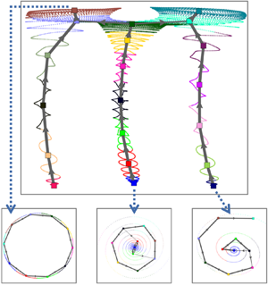
We consider the two-dimensional incompressible flow configuration of Bansal & Yarusevych (Reference Bansal and Yarusevych2017), defined as the unforced ‘fluidic pinball’ in Deng et al. (Reference Deng, Noack, Morzyski and Pastur2020). With increasing Reynolds number, the wake undergoes a first instability leading to a periodic vortex shedding, then a static symmetry breaking and finally a transition to a quasi-periodic regime before transiting to a chaotic regime. HiCNMs are built for these flow regimes, which have multiple invariant sets and exhibit different transient dynamics. We provide a principle sketch of our HiCNM framework in figure 1.

Figure 1. Overview of the cluster-based hierarchical network modelling framework exemplified at  $Re=80$. (a) The flow dynamics involves six invariant sets associated with three unstable fixed points, three limit cycles, as shown in the three-dimensional phase portrait of the drag and lift forces. (b) Under the mean-field consideration, the flow can be decomposed into a slowly varying mean flow, the coherent and incoherent components, separated by the dominant frequency of the coherent part. The non-coherent fluctuating component is weak in this case, and the third term of the triple decomposition can be ignored. (c) Therefore, a HiCNM with two layers is enough to extract the global trend and the local dynamics of the varying mean-flow field. The transient and post-transient dynamics, characterized by multiple frequencies and multiple invariant sets, are introduced in § 2.2. The hierarchical network modelling strategy is discussed in § 3.2.2 under the mean-filed consideration in § 3.1.1. The dynamics reconstruction of the resulting hierarchical network model is given in § 3.2.3.
The manuscript is organized as follows: § 2 describes the numerical plant of the fluidic pinball and the flow features at different Reynolds number. Section 3 discusses the different perspectives on the cluster-based hierarchical network modelling strategy. In § 4, we discuss the HiCNMs applied to the transient and post-transient dynamics of a flow configuration involving six invariant sets, for three different Reynolds numbers, respectively associated with a periodic, a quasi-periodic and a chaotic dynamics. Section 5 summarizes the main findings and gives some suggestions for improvement and future directions.
2. Flow configuration and flow features
We consider two-dimensional incompressible flows in the fluidic pinball (Noack & Morzyński Reference Noack and Morzyński2017) as the benchmark configuration for our hierarchical modelling strategy. The flow configuration and the direct Navier–Stokes solver are described in § 2.1. The transient and post-transient dynamics at different Reynolds numbers are illustrated in § 2.2.
2.1. Flow configuration and direct Navier–Stokes solver
Figure 2 shows the geometric configuration of the fluidic pinball, consisting of three fixed cylinders of unit diameter  $D$. Their axes are placed on the vertices of an equilateral triangle of side $3D/2$ in the $(x, y)$ plane. The upstream flow is in the $x$-axis direction with a uniform velocity $U_\infty$ at the inlet of the domain. The computational domain $\varOmega$ is bounded by a rectangular box of size $[-6D,+20D] \times [-6D,+6D]$. A Cartesian coordinate system is used for description, and its origin is placed in the middle of the back two cylinders considering the symmetry of this configuration. Since no external force is applied to these three cylinders, a no-slip condition is applied on the cylinders, and the velocity in the far wake is assumed to be $U_\infty$. The Reynolds number is defined as $Re = U_\infty D/\nu$, where $\nu$ is the kinematic viscosity of the fluid. A no-stress condition is applied at the outlet of the domain.

Figure 2. Configuration of the fluidic pinball and computational grid for the simulated domain. The upstream velocity is denoted  $U_\infty$. An example vorticity field at $Re=130$ is colour coded in the range $[-1.5, 1.5]$ from blue to red.
The fluid flow is governed by the non-dimensionalized incompressible Navier–Stokes equations in scales with the cylinder diameter  $D$ and the velocity $U_\infty$, which read
 \begin{equation} \partial_t \boldsymbol{u} + \boldsymbol{\nabla} \boldsymbol{\cdot} \boldsymbol{u} \otimes \boldsymbol{u} = \nu \triangle \boldsymbol{u} - \boldsymbol{\nabla} p, \quad \boldsymbol{\nabla} \boldsymbol{\cdot} \boldsymbol{u}=0, \end{equation}
where  $p$ and $\boldsymbol {u}$ are respectively the pressure and velocity flow fields and $\nu = 1/Re$. The advection time scale is $D/U_\infty$ and the pressure scale is $\rho U^2_\infty$, where $\rho$ is the unit fluid density for the incompressible flow. It is assumed that there exists a solution $(\boldsymbol {u}_s,p_s)$ satisfying the steady Navier–Stokes equations
 \begin{equation} \boldsymbol{\nabla} \boldsymbol{\cdot} \boldsymbol{u}_s \otimes \boldsymbol{u}_s = \nu \triangle \boldsymbol{u}_s - \boldsymbol{\nabla} p_s, \quad \boldsymbol{\nabla} \boldsymbol{\cdot} \boldsymbol{u}_s=0. \end{equation}
The inner product of two square-integrable velocity fields  $\boldsymbol {u} (\boldsymbol {x})$ and $\boldsymbol {v} (\boldsymbol {x})$ in the computational domain $\varOmega$ reads
 \begin{equation} ( \boldsymbol{u} , \boldsymbol{v} )_{\varOmega} := \int_{\varOmega} {\rm d}\kern0.7pt \boldsymbol{x} \boldsymbol{u}(\boldsymbol{x}) \boldsymbol{\cdot} \boldsymbol{v}(\boldsymbol{x}). \end{equation}
The associated norm of the velocity field  $\boldsymbol {u}(\boldsymbol {x})$ is defined as
 \begin{equation} \|\boldsymbol{u}\|_{\varOmega}:= \sqrt{( \boldsymbol{u} , \boldsymbol{u} )_{\varOmega}}. \end{equation}
The direct numerical simulation (DNS) of the Navier–Stokes equations (2.1a,b) is based on a second-order finite-element discretization method of the Taylor–Hood type (Taylor & Hood Reference Taylor and Hood1973), on an unstructured grid of 4225 triangles and 8633 vertices, and an implicit integration of the third-order in time. The unsteady flow field is calculated by an unsteady solver with Newton–Raphson iteration until the residual is less than a prescribed tolerance. This approach is also employed to calculate the steady solution by a steady solver for the steady Navier–Stokes equations (2.2a,b). The direct Navier–Stokes solver used herein has been validated in Noack et al. (Reference Noack, Afanasiev, Morzyński, Tadmor and Thiele2003) and Deng et al. (Reference Deng, Noack, Morzyski and Pastur2020), and the grid used for the simulations provides a consistent flow dynamics compared with a refined grid. A relevant numerical investigation for this kind of equilateral-triangle configuration can also be found in Chen et al. (Reference Chen, Ji, Alam, Williams and Xu2020). The data-driven HiCNM method is exemplified on this benchmark configuration with a blockage ratio  $B=0.21$, defined as the ratio of the cross-section length of the cluster of three cylinders $5D/2$ to the width of the computational domain $12D$, which mimics the experimental set-ups in Raibaudo et al. (Reference Raibaudo, Zhong, Noack and Martinuzzi2020). The numerical results with the current computational domain remain similar compared with a larger domain with $B=0.025$, as detailed in Appendix A.
2.2. Flow features
As shown in figure 3, the flow undergoes a supercritical Hopf bifurcation at  $Re_1\approx 18$, a supercritical pitchfork bifurcation at $Re_2\approx 68$ and a Neimark–Säcker bifurcation at $Re_3\approx 105$, before entering the chaotic regime beyond $Re_4\approx 115$ with increasing Reynolds number (Deng et al. Reference Deng, Noack, Morzyski and Pastur2020). Depending on the Reynolds number, the wake flow may present a rich transient dynamics due to multiple exact solutions of the Navier–Stokes equations, associated with the co-existing invariant sets in the state space. For instance, for $Re_1< Re< Re_2$, the symmetric steady solution $\boldsymbol {u}_s$ is the only fixed point of the system. This exact solution of the Navier–Stokes equations is unstable. The only attractor in the state space is a symmetric limit cycle, associated with the cyclic release of vortices in the wake of the cylinders, forming a von Kármán street of regular vortices. For $Re>Re_2$, three fixed points are solutions of the steady Navier–Stokes equations, one symmetric $\boldsymbol {u}_s$ and two asymmetric steady solutions $\boldsymbol {u}_s^{\pm }$, and all three points are unstable. Meanwhile, the unsteady Navier–Stokes equations have three periodic solutions. The symmetric limit cycle, associated with symmetric vortex shedding, is unstable. The two mirror-conjugated asymmetric limit cycles, associated with asymmetric vortex sheddings, co-exist as attractors of the flow dynamics in the state space. For $Re_3< Re< Re_4$, the two attracting asymmetric limit cycles thicken into tori by introducing an additional low frequency, which modulates the vortex shedding quasi-periodically. Beyond $Re_4$, the vortex shedding dynamics is chaotic. The interested reader can find more details on the route to chaos in the fluidic pinball in Deng et al. (Reference Deng, Noack, Morzyski and Pastur2020).
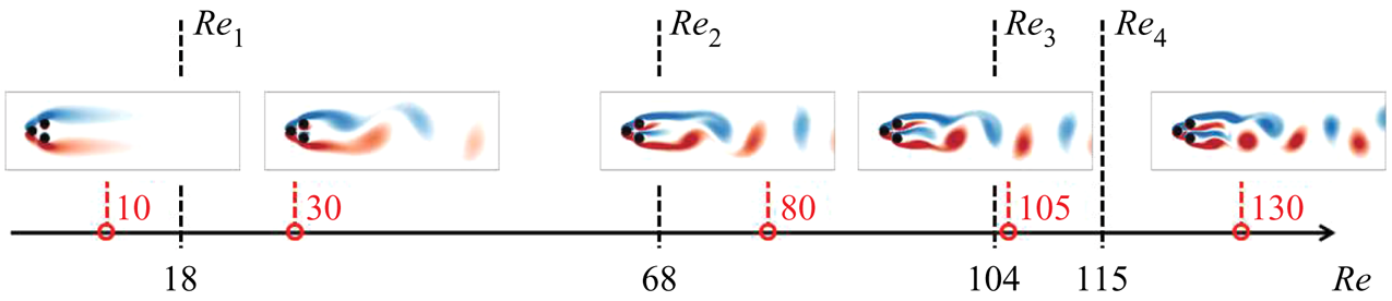
Figure 3. Post-transient flow state for different flow regimes at the Reynolds numbers marked in red. The critical values of the supercritical Hopf bifurcation  $Re_1$, the supercritical pitchfork bifurcation $Re_2$ and the Neimark–Säcker bifurcation $Re_3$ before the system entering into chaos at $Re_4$ are marked in black on the $Re$-axis.
The flow features can be illustrated by the forces exerted on the body. The drag  $F_D$ and lift $F_L$ forces are the projection on $\boldsymbol {e}_x$ and $\boldsymbol {e}_y$ of the resultant force $\boldsymbol {F} =F_D \boldsymbol {e}_x + F_L \boldsymbol {e}_y$, obtained by integrating the viscous and pressure forces over the cylinder surfaces. The flow dynamics is analysed with the lift coefficient $C_L$,
 \begin{equation} C_L (t)= \frac{2F_L (t)}{\rho U_\infty^2}. \end{equation}
 We apply the DNSs at  $Re = 30, 80, 105$ and $130$ starting close to the symmetric steady solution (for $Re>Re_1$) until $t=1500$ and the asymmetric steady solutions (for $Re>Re_2$) until $t=1000$. The time evolutions of the lift coefficient $C_L$ are shown in figure 4, where different transient dynamics are observed, from the steady solutions to the asymptotic regimes.

Figure 4. Transient and post-transient dynamics starting with different steady solutions, illustrated with the time evolution of the lift coefficient  $C_L$ at $Re = 30$ (a), $80$ (b), $105$ (c), $130$ (d).
At  $Re = 30$, as shown in figure 4(a), the lift coefficient $C_L$ starts to oscillate visibly at $t \approx 800$, indicating that the flow leaves the neighbourhood of the symmetric steady solution. Then, $C_L$ oscillates around a vanishing value with increasing amplitude until converging to a fixed amplitude. This state refers to a symmetric vortex shedding, as the instantaneous flow is oscillating around a geometrical symmetric mean-flow field.
At  $Re = 80$, as shown in figure 4(b), the primary transition is the same as at $Re=30$. Next, the slowly varying mean lift coefficient $\langle C_L\rangle _T$, averaged over the oscillation period $T$, goes from $0$ to $0.04$. This indicates that the oscillatory dynamics in the permanent regime has lost the statistical symmetry, and the flow state refers to an asymmetric vortex shedding. Starting nearby either one of the two asymmetric steady solutions, $C_L$ directly evolves to the asymmetric vortex shedding regime that shares the same asymmetry.
At  $Re = 105, C_L$ visibly increases at $t \approx 580$ starting with the vanishing value of the symmetric steady solution, as illustrated with the black curve in figure 4(c). However, the initial transition reaches a non-oscillating value equal to the initial value of the red curve, which refers to one of the two asymmetric steady solutions. It eventually enters a quasi-periodic state, the vortex shedding oscillations being modulated at a low frequency. Starting from the other two asymmetric steady solutions will directly evolve into the permanent quasi-periodic state with the same asymmetry.
At  $Re = 130$, the initial transition of the black curve in figure 4(d) is similar to the initial transition at $Re = 80$, but the dynamics enters a chaotic regime shortly after the symmetric vortex shedding has started. Simulations converge to the same chaotic attracting set, starting with all the three different steady solutions.
3. Cluster-based hierarchical reduced-order modelling
In this section, the general approach of the cluster-based hierarchical reduced-order modelling is described and discussed. In § 3.1, we present the relevant background on the flow decomposition and the standard CROM. The cluster-based reduced-order modelling with hierarchical structure is described in § 3.2, as well as the relevant analysis of the HiCNM.
3.1. Background
The standard CROM is obtained in two steps: the snapshots are first clustered into coarse-grained representative states before building either a Markov or a network model for the analysis of the dynamics. Clustering all transients and post-transients at once can suffer from the inability to accurately capture the dynamics at different scales. Under the mean-field consideration, we introduce a hierarchical structure of clusters for the flow dynamics of different time scales, resulting in a cluster-based hierarchical reduced-order model (HiCROM).
3.1.1. Flow decomposition with mean-field consideration
The starting point of the HiCROM is the triple decomposition of the flow field similar to Reynolds & Hussain (Reference Reynolds and Hussain1972)
 \begin{equation} \boldsymbol{u} (\boldsymbol{x}, t) = \underbrace{ \langle \boldsymbol{u} (\boldsymbol{x},t)\rangle _T }_{\omega \ll \omega_c} + \underbrace{ \tilde{\boldsymbol{u}} ( \boldsymbol{x}, t) }_{\omega \sim \omega_c} + \underbrace{ \boldsymbol{u}^{\prime} ( \boldsymbol{x}, t) }_{\omega \gg \omega_c}, \end{equation}
where the dominant angular frequency  $\omega _c$ is defined as the dominant peak in the Fourier spectrum of the velocity field. Here, the velocity field is decomposed into a slowly varying mean-flow field $\langle \boldsymbol {u}\rangle _T$, a coherent component on time scales of order $2{\rm \pi} /\omega _c$, involving coherent structures $\tilde {\boldsymbol {u}}$, and the remaining non-coherent small scale fluctuations $\boldsymbol {u}^{\prime }$. This kind of decomposition can also be found in the low-order Galerkin models of Tadmor et al. (Reference Tadmor, Lehmann, Noack, Cordier, Delville, Bonnet and Morzyński2011) and the weakly nonlinear modelling of Rigas, Morgans & Morrison (Reference Rigas, Morgans and Morrison2017a).
The slowly varying mean-flow field  $\langle \boldsymbol {u}\rangle _T$ can be defined as the average of the velocity field $\boldsymbol {u}$ over one local period $T\approx 2{\rm \pi} /\omega _c$ of the coherent structures,
 \begin{equation} \langle \boldsymbol{u} ( \boldsymbol{x}, t ) \rangle _T := \frac{1}{T} \int_{t-T/2}^{t+T/2} \, {\rm d} \tau \boldsymbol{u} (\boldsymbol{x}, \tau ), \end{equation}
which eliminates both the coherent contribution from  $\tilde {\boldsymbol {u}}$ and the non-coherent contribution from $\boldsymbol {u}^{\prime }$. Unlike the mean-flow field defined by the post-transient limit,
 \begin{equation} \bar{\boldsymbol{u}} (\boldsymbol{x}) = \lim_{T\rightarrow \infty }\frac{1}{T}\int_{0}^{T} \boldsymbol{u} (\boldsymbol{x}, \tau) \, {\rm d} \tau, \end{equation}
the finite-time-averaged flow field considered in this study owns a slowly varying dynamics. From the mean-field theory of Stuart (Reference Stuart1958), the slowly varying mean-flow field evolves out of the steady solution under the action of the Reynolds stress associated with the most unstable eigenmode(s). The mean-flow field deformation  $\boldsymbol {u}_{\varDelta }$ is used to describe the difference between the slowly varying mean-flow field and the invariant steady solution $\boldsymbol {u}_s (\boldsymbol {x})$, which reads
 \begin{equation} \langle \boldsymbol{u} (\boldsymbol{x},t)\rangle _T = \boldsymbol{u}_s (\boldsymbol{x}) + \boldsymbol{u}_{\varDelta} (\boldsymbol{x},t). \end{equation}
3.1.2. Clustering algorithm
We consider the state vectors, for instance, the velocity fields  $\boldsymbol {u} (\boldsymbol {x},t)$ in the computational domain $\varOmega$, which is sampled at times $t^m = m\Delta t$ with a time step $\Delta t$, where the superscript $m=1,\ldots,M$ is the snapshot index. The clustering process aims at partitioning the $M$ time-discrete states (snapshots) $\boldsymbol {u}^m = \boldsymbol {u} (\boldsymbol {x},t^m)$ into $K$ clusters $\mathcal {C}_k, k = 1,\ldots,K$. Snapshots of a given cluster share similar attributes featured by its cluster centroid $\boldsymbol {c}_k$. The distance between the snapshot $\boldsymbol {u}^m$ and the centroid $\boldsymbol {c}_k$ is defined as
 \begin{equation} D^{m}_{k}:= \|\boldsymbol{u}^m - \boldsymbol{c}_k\|_{\varOmega}. \end{equation}
Each snapshot is partitioned to the cluster of the closest centroid by  $\hbox {argmin}_k D^{m}_{k}$, and the characteristic function is defined as
 \begin{equation} \chi_{k}^{m} := \begin{cases} 1, & \mbox{if }\boldsymbol{u}^m\in \mathcal{C}_k,\\ 0, & \mbox{otherwise}. \end{cases}\end{equation}
A cluster index  $k^m, m=1,\ldots,M$, indicates the cluster assignment of the corresponding snapshot with $\boldsymbol {u}^m \in \mathcal {C}_k$, and records the visited clusters consecutively. The number of snapshots $n_k$ in cluster $k$ is given by
 \begin{equation} n_k = \sum_{m=1}^M \chi_{k}^{m}.\end{equation}
The cluster centroids  $\boldsymbol {c}_k$ are defined as the average of the snapshots belonging to the cluster $\mathcal {C}_k$:
 \begin{equation} \boldsymbol{c}_k= \frac{1}{n_k} \sum_{m=1}^M \chi_{k}^{m} \boldsymbol{u}^m. \end{equation}
The performance of clustering is judged by the within-cluster variances
 \begin{equation} J (\boldsymbol{c}_1,\ldots,\boldsymbol{c}_K ) = \sum_{k=1}^K \sum_{m=1}^M \chi_{k}^{m}\Vert\boldsymbol{u}^m - \boldsymbol{c}_k \Vert_{\varOmega}^2. \end{equation}
The clustering algorithm minimizes  $J$ and determines the optimal centroid positions,
 \begin{equation} \boldsymbol{c}_1^{{opt}}, \ldots,\boldsymbol{c}_K^{{opt}} = \hbox{argmin}_{\boldsymbol{c}_1,\ldots,\boldsymbol{c}_K}\, J (\boldsymbol{c}_1,\ldots,\boldsymbol{c}_K ), \end{equation}
by iteratively updating the characteristic function and the centroid positions.
To solve the optimization problem (3.10), we use the  $k$-means $++$ algorithm (Arthur & Vassilvitskii Reference Arthur and Vassilvitskii2006). Comparing with the traditional $k$-means algorithm, the $k$-means $++$ algorithm selects the initial centroids as far away as possible to avoid any bias from the initial conditions. The remaining steps of the two algorithms are the same. At each iteration, the snapshots are divided into clusters of the nearest newly determined centroids. The optimal centroids are obtained by iterating until either convergence or when the maximum number of iterations is reached.
3.1.3. Cluster-based network model
Based on the clustering result, Kaiser et al. (Reference Kaiser, Noack, Cordier, Spohn, Segond, Abel, Daviller, Östh, Krajnović and Niven2014) derived a CMM, which provides a probabilistic representation of the system using a Markov process, with the assumption that the fluid system is memoryless. Nair et al. (Reference Nair, Yeh, Kaiser, Noack, Brunton and Taira2019) removed the transitions residing in the same cluster and emphasized the non-trivial transitions between two different clusters. In these two works, the transitions are only characterized by probabilities. The CNM proposed in Fernex et al. (Reference Fernex, Noack and Semaan2021) and Li et al. (Reference Li, Fernex, Semaan, Tan, Morzyński and Noack2021), inherited the idea of focusing on the non-trivial transitions, and further introduced time scale characteristics by recording the transition times. We here briefly review some concepts of the CNM, as they will be used in our benchmark of HiCNM.
The  $M$ consecutive snapshots define $M-1$ transitions, containing trivial transitions staying in the same cluster and non-trivial transitions between two different clusters. The number of transitions from $\mathcal {C}_j$ to $\mathcal {C}_i$ reads
 \begin{equation} n_{ij} = \sum_{m=1}^{M-1} \chi_{j}^{m} \chi_{i}^{m+1}. \end{equation}
Considering the non-trivial transitions,  ${n_{j}}$ is the total number of departing snapshots from $\mathcal {C}_j$, with $n_j = \sum _{i=1}^K (1-\delta _{ij}) n_{ij}$. The direct transition probability $P_{ij}$ reads
 \begin{equation} P_{ij}= \frac{(1-\delta_{ij}) n_{ij}}{n_{j}}, \quad i, j = 1, \ldots, K, \end{equation}
where the non-migrating transition  ${n_{jj}}$ is eliminated. All the non-trivial transitions are identified with the direct transition matrix ${\boldsymbol{\mathsf{P}}}$.
The residence time matrix  ${\boldsymbol{\mathsf{T}}}$ relies on the time information of the snapshots. After clustering, each snapshot $\boldsymbol {u}^m= \boldsymbol {u}(t^m)$ is associated with the closest centroid with a cluster index $k^m$. Assuming that $N$
$N$  $(N < M)$ non-trivial transitions occur along the trajectory, the moments of transition $t_n, n=1,\ldots,N$ – including the initial time $t_0=t^1$ – are defined as the time entering into a new cluster,
 \begin{equation} t_n = t^m \mbox{ if }\boldsymbol{u}^{m-1}\in \mathcal{C}_k \ \& \ \boldsymbol{u}^{m} \notin \mathcal{C}_k, \end{equation}
with ascending order  $t_0 < t_1 < \cdots < t_N$. The cluster index $k^m$ remains unchanged in a time range $[t_n, t_{n+1} )$. The sequence of visited clusters over time can be simplified with the first entering snapshot for each non-trivial transition with $k^m$ taken from the moments of transition $t_n$.
For a simple transition from  $\mathcal {C}_j$ to $\mathcal {C}_i$ as illustrated in figure 5, where the trajectory first enters in $\mathcal {C}_j$ at time $t_{n}$, and leaves $\mathcal {C}_j$ for $\mathcal {C}_i$ at time $t_{n+1}$, the residence time in $\mathcal {C}_j$ is defined as
 \begin{equation} T_{ij}:= t_{n+1} - t_{n}. \end{equation}
In the case of multiple trajectories of transition from  $\mathcal {C}_j$ to $\mathcal {C}_i$, the residence time will be averaged according to the number of trajectories.

Figure 5. An illustration of the residence time in the cluster-based network model;  $\bullet$ remarks the entering time into new clusters.
At this point, the time-resolved snapshots  $\boldsymbol {u}^m$ can be represented by cluster centroids $\boldsymbol {c}_{k^m}$ with the time evolution of the cluster index $k^m$. The transient dynamics is described by both the direct transition matrix of non-migrating transitions ${\boldsymbol{\mathsf{P}}}$ and the residence time matrix ${\boldsymbol{\mathsf{T}}}$.
3.2. Hierarchical modelling with mean-field consideration
As introduced in figure 1, the framework of cluster-based hierarchical network modelling contains the following three steps. The hierarchical clustering with mean-field consideration is introduced in § 3.2.1. Based on the identified clusters, the network modelling with hierarchical structure is derived in § 3.2.2 for the mean-field model of (3.1) under a small number of general assumptions. Section 3.2.3 introduces the autocorrelation function and its root mean square error of the rebuilt flow for the validation of the HiCNM. An introductory example is introduced in Appendix B.1 to clarify the primary form of the HiCNM.
3.2.1. Hierarchical clustering inspired by the triple decomposition
To better understand the global and local properties of the data, we present a novel hierarchical clustering algorithm inspired by the triple decomposition introduced in § 3.1.1. The principle of hierarchical clustering is to divide the snapshots into layers of clusters. Snapshots belonging to clusters of the parent layer are further partitioned into clusters of the child layer. Hierarchical clustering algorithms are generally divided into two categories:
(a) The agglomerating (‘bottom-up’) hierarchical clustering begins with the smallest clusters at the bottom, each snapshot being an elementary cluster. The two closest clusters are merged to generate a new cluster according to certain criteria, introducing an additional layer from the bottom. This merging is repeated until all snapshots belong to one cluster at the top of the hierarchy.
(b) The divisive (‘top-down’) hierarchical clustering starts with only one cluster, which owns all the snapshots. In our case, the centroid of the top cluster would be the mean-flow field from ensemble averaging. From the top to the bottom, the snapshots in each cluster of the parent layer are divided into multiple clusters in the child layer, according to certain criteria. The bottom layers will be associated with the small scale fluctuations of the flow field. The division can be continued until each snapshot is a cluster.
We employ a divisive hierarchical clustering to distil the different features in a hierarchy, which is consistent with the triple decomposition of (3.1). For instance, fluid flows characterized by multiple frequencies require only a finite number of layers to describe the different components bounded by frequency.
Transient and post-transient dynamics are statistically non-homogeneous due to the existence of multiple invariant sets. If so, a scale sub-division of the flow-field decomposition like in (3.1) is used during the clustering process. Accounting for the Reynolds stress contribution, the slowly varying mean-flow field  $\langle \boldsymbol {u}\rangle _T$ is enough to describe the global trend. Next, the local dynamics around $\langle \boldsymbol {u}\rangle _T$ can be zoomed in, considering the coherent structures involved in $\tilde {\boldsymbol {u}}$. This scale sub-division can still be extended to a hierarchical structure with more layers, which involve secondary frequencies in the case of quasi-periodic dynamics or turbulence from $\boldsymbol {u}^{\prime }$, as illustrated in figure 6. In order to clearly describe the clusters in the hierarchy, we systematically name the clusters from top to bottom. The sole cluster on the top $\mathcal {L}_0$ contains the ensemble of input data, and we define it symbolically as $\mathcal {C}_0$. The sub-division of this cluster leads to $K_1$ subclusters in the first layer $\mathcal {L}_1$, named as $\mathcal {C}_{0, k_1}, k_1=1,\ldots, K_1$. The first subscript $k_0 = 0$ can be ignored because there is only one cluster in $\mathcal {L}_0$, and the second subscript $k_1$ indicates the index of the subcluster in $\mathcal {L}_1$. The second sub-division works on each cluster $\mathcal {C}_{k_1}$ separately, and generates refined $K_2$ subclusters for each of them. The cluster index in the current layer $\mathcal {L}_2$ is presented by an additional subscript $k_2 = 1, \ldots, K_2$, which is written as $\mathcal {C}_{k_1, k_2}$. For a higher layer number $\mathcal {L}_{L \in \mathbb {N}}, L \geqslant 3$, more subscripts $k_L, l = 1, \ldots, L$, are needed to record the cluster index in each layer $\mathcal {L}_l$ from the top to the bottom, written as $\mathcal {C}_{k_1, \ldots, k_L}$. This naming method can clearly trace out all clusters in the hierarchy, and also works for other properties of clusters, e.g. the centroids $\boldsymbol {c}_{k_1, \ldots, k_L}$ and the characteristic function $\chi _{k_1, \ldots, k_L}^{m}$. In this work, two or three layers ( $L \leqslant 3$) will be enough to extract the transient dynamics out of multiple invariant sets.

Figure 6. An illustration of the hierarchical structure with different scales in the triple flow decomposition in § 3.1.1. Layer 0: the top layer is characterized by the invariant mean flow  $\bar {\boldsymbol {u}}$. Layer 1: the global trend is described by the slowly varying mean-flow field $\langle \boldsymbol {u}\rangle _T$. Layer 2: the coherent part $\tilde {\boldsymbol {u}}$ is added for the local dynamics around the varying mean-flow field. Layer 3: the non-coherent part $\boldsymbol {u}^{\prime }$ is considered in the case of turbulent flow.
3.2.2. Hierarchical network modelling
The starting point is the hierarchical Markov model of Fine et al. (Reference Fine, Singer and Tishby1998), which introduces the hierarchical structure to describe the stochastic processes, comparing with the standard Markov model. Each state of a Markov model in the parent layer is considered separately, and a new Markov model of the sub-states of a state is built in the child layer. As the layer increases, the state is continuously sub-divided. Therefore, the hierarchical Markov model records a sequence of states in different layers. In our case, each cluster is seen as a state. When a cluster in the parent layer is activated, its subclusters in the child layer turns activated recursively. Meanwhile, the refined dynamics between the subclusters can be described by a Markov model. Hence, the hierarchical Markov model can more effectively solve the problem of subsets.
In this work, we derive the HiCNM by replacing the Markov model by the network model. The hierarchical structure is identical, and the only change is the way to describe the transient dynamics between clusters.
A typical structure between the parent and child layers is shown in figure 7. We start with cluster  $\mathcal {C}_{k_1 , \ldots, k_{l-1} }$ in the parent layer $\mathcal {L}_{l-1}$, where the leading subscript $k_1 , \ldots, k_{l-2}$ refers to the cluster number in each upper layer. For convenience, when the context is unambiguous, the cluster will be only referenced by its number in the current layer, e.g. $\mathcal {C}_{k_{l-1}}$. As indicated with the sequence of cluster numbers in its complete name, this cluster comes from the sub-division of the cluster $\mathcal {C}_{k_1 , \ldots, k_{l-2} }$ in the parent layer $\mathcal {L}_{l-2}$. We suppose that $M$ snapshots $\boldsymbol {u}^{m}, m=1,\ldots,M$, exist in this cluster and are divided into $K_{l-1}$ subclusters by a sub-division clustering algorithm. The subcluster $\mathcal {C}_{k_{l-1}}$ contains $n_{k_{l-1} }$ snapshots, calculated from (3.7) with the characteristic function $\chi _{k_{l-1} }^{m}$. A standard network model for the cluster $\mathcal {C}_{k_1 , \ldots, k_{l-2} }$ can be derived with the direct transition matrix ${\boldsymbol{\mathsf{P}}}_{k_1 , \ldots, k_{l-2} }$ and the residence time matrix ${\boldsymbol{\mathsf{T}}}_{ k_1 , \ldots, k_{l-2} }$, as recorded in § 3.1.3, which describe the dynamics between the subclusters $\mathcal {C}_{k_{l-1}}$.

Figure 7. An illustration of the transitions between the parent and child layers in the hierarchical network model. The trajectories pass through the cluster in the parent layer: the entering and exiting snapshots are marked with red dot and the blue dot. After clustering, a classic network model is built between  $N$ subclusters, with transition probability $P$. The vertical transitions indicate the ports of entry and exit of the subclusters with probabilities $Q_{o,j}$ and $Q_{e,j}$.
In the following, we focus on the trajectories passing through cluster  $\mathcal {C}_{k_{l-1}}$. The snapshots entering and leaving from $\mathcal {C}_{k_{l-1}}$ are marked out for each trajectory, with the following characteristic function:
 \begin{equation}
\left.\begin{array}{c@{}}
\chi_{o, k_{l-1}}^{m} := \begin{cases}
1, & \mbox{if }\boldsymbol{u}^{m-1} \notin \mathcal{C}_{k_{l-1}} \ \& \ \boldsymbol{u}^{m} \in \mathcal{C}_{k_{l-1}}, \\
0, & \mbox{otherwise}.
\end{cases} \\
\chi_{e, k_{l-1}}^{m} := \begin{cases}
1, & \mbox{if }\boldsymbol{u}^{m}\in \mathcal{C}_{k_{l-1}} \ \& \ \boldsymbol{u}^{m+1} \notin \mathcal{C}_{k_{l-1}}, \\
0, & \mbox{otherwise}.
\end{cases}
\end{array}\right\}
\end{equation}
\begin{equation}
\left.\begin{array}{c@{}}
\chi_{o, k_{l-1}}^{m} := \begin{cases}
1, & \mbox{if }\boldsymbol{u}^{m-1} \notin \mathcal{C}_{k_{l-1}} \ \& \ \boldsymbol{u}^{m} \in \mathcal{C}_{k_{l-1}}, \\
0, & \mbox{otherwise}.
\end{cases} \\
\chi_{e, k_{l-1}}^{m} := \begin{cases}
1, & \mbox{if }\boldsymbol{u}^{m}\in \mathcal{C}_{k_{l-1}} \ \& \ \boldsymbol{u}^{m+1} \notin \mathcal{C}_{k_{l-1}}, \\
0, & \mbox{otherwise}.
\end{cases}
\end{array}\right\}
\end{equation}
The entering snapshots are denoted by the subscript ‘ $o$’, and the exiting snapshots by the subscript ‘ $e$’. The number of entering snapshots $n_o$ and of exiting snapshots $n_e$ read
 \begin{equation} n_o = \sum_{m=1}^M \chi_{o,k_{l-1}}^{m}, \quad n_e = \sum_{m=1}^M \chi_{e,k_{l-1}}^{m}. \end{equation}
 In the child layer  $\mathcal {L}_{l}$, the $n_k$ snapshots in the cluster $\mathcal {C}_{k_{l-1}}$ have been divided into the subclusters $\mathcal {C}_{k_1 , \ldots, k_{l} }$ , $k_{l} =1,\ldots,k_L$. Without loss of generality, a standard network model for the cluster $\mathcal {C}_{k_{l-1}}$ can be built with its subclusters with the direct transition matrix ${\boldsymbol{\mathsf{P}}}_{k_1 , \ldots, k_{l-1} }$ and the residence time matrix ${\boldsymbol{\mathsf{T}}}_{ k_1 , \ldots, k_{l-1} }$.
The snapshots  $\boldsymbol {u}^m$ are approximated by the time evolution of the cluster centroids $\boldsymbol {c}_{k_1^m, \ldots, k_{l}^m }$ in $\mathcal {L}_{l}$,
 \begin{equation} \hat{\boldsymbol{u}}^m_{\mathcal{L}_{l}} = \boldsymbol{c}_{k_1^m, \ldots , k_{l}^m }. \end{equation}
The residence time elements of  ${\boldsymbol{\mathsf{T}}}_{k_1 , \ldots, k_{l}}$ can be assembled in order to determine the moments of transition based on the sequence of visited clusters in $\mathcal {L}_{l}$.
The entering and exiting snapshots defined in (3.15) can be used to describe the vertical transitions. Although they are not necessary to describe the dynamics of the fluidic pinball, the probability of the vertical transitions  $Q_{o,j}$ and $Q_{e,j}$, described in Appendix B, completes all possible transitions in our hierarchical structure and makes it consistent with the classic hierarchical Markov model of Fine et al. (Reference Fine, Singer and Tishby1998).
3.2.3. Dynamics reconstruction of the hierarchical network model
The reconstructed flow in (3.17) is a statistical representation of the original snapshot sequence by a few representative centroids, which is a highly discretized description compared with the full dynamics. The approximations in the different layers provide different metrics for the flow dynamics.
The cluster-based hierarchical model uses the centroids  $\boldsymbol {c}_{k_1^m, \ldots, k_{l}^m }$ in the original data space together with the time evolution of the cluster index $k_{l}^m$ to simplify the description of the original flow, which is more intuitive and closer to the original flow than the POD reconstruction. For input data with $I$-dimensional state vectors of the velocity field and $M$ snapshots, a POD reconstruction truncated to $R$ modes will lead to a $I \times R$ matrix of POD modes and a $R \times M$ matrix of mode amplitudes. A HiCNM with $K$ centroids leads to a $I \times K$ matrix of centroids and a sequence of the $N$ visited clusters of length $N \ll M$. In this sense, the compressive ability of HiCNM is more powerful for the large amount of continuously sampled data, as $I \times K < (I+M)\times R$. In addition, the hierarchical clustering works as a sparse sampling technique, extracting the representative states according to the clustering subspace.
We use the unbiased auto-correlation function (Protas, Noack & Östh Reference Protas, Noack and Östh2015),
 \begin{equation} R(\tau)=\frac{1}{T-\tau}\int_{\tau}^{T}(\boldsymbol{u}(\boldsymbol{x}, t-\tau) - \boldsymbol{u}_s(\boldsymbol{x}),\boldsymbol{u}(\boldsymbol{x}, t)- \boldsymbol{u}_s(\boldsymbol{x}))_{\varOmega} \mathrm{d}t, \quad \tau\in [0,T), \end{equation}
after normalization with respect to  $R(0)$ to check the accuracy of the dynamics reconstruction of the HiCNM in (3.17). The autocorrelation function without delay $R(0)$ is twice the time-averaging kinetic energy. The modelled autocorrelation function $\hat {R}_{\mathcal {L}_{l}}(\tau )$ in layer $\mathcal {L}_{l}$ is based on the rebuilt flow $\hat {\boldsymbol {u}}_{\mathcal {L}_{l}}$ in (3.17) instead of $\boldsymbol {u}$ in (3.18).
For the discrete snapshots, the root mean-square error (RMSE) of the autocorrelation function  $R(\tau )$ of the reference data and that of the model $\hat {R}_{\mathcal {L}_{l}}(\tau )$ is defined as
 \begin{equation} R_{rms}^l : = \sqrt{\frac{1}{M}\sum_{m=1}^{M}(R(\tau)-\hat{R}_{\mathcal{L}_{l}}(\tau))^2}, \end{equation}
where  $M$ is the number of snapshots $\boldsymbol {u}^m$ and $\hat {\boldsymbol {u}}^m_{\mathcal {L}_{l}}$ at $\tau = m \Delta t$.
4. Hierarchical network modelling of the fluidic pinball
In this section, we apply the hierarchical modelling strategy to the fluidic pinball at different Reynolds numbers. With increasing Reynolds number, the flow dynamics undergoes successive instabilities and bifurcations, introducing multiple exact solutions of the Navier–Stokes equations and multiple invariant sets for the dynamics. In § 4.1, the modelling strategy dealing with multiple invariant sets is introduced. We derive the HiCNMs for the transient dynamics involving six invariant sets at  $Re=80$ in § 4.2, for the quasi-periodic regime at $Re=105$ in § 4.4 and for the chaotic regime at $Re=130$ in § 4.5.
4.1. Hierarchical modelling with multiple invariant sets
The flow field is computed with the DNS described in § 2.1. The resulting flow field is an ensemble of time-resolved snapshots starting with some given initial condition. The transient and post-transient dynamics of the flow constitute a time-resolved trajectory sampled with a fixed time step. Different invariant sets and multiple attractors can co-exist in the state space, only part of them being explored by each individual trajectory from the initial condition to the asymptotic regime. All the cases of interest in this paper are such that  $Re>Re_2$, i.e. beyond the supercritical pitchfork bifurcation. The data set consists of the snapshots computed from four different trajectories: two mirror-conjugated trajectories starting in the vicinity of the symmetric steady solution, the two others starting from the two mirror-conjugated asymmetric steady solutions. The simulations are respectively run until $t=1500$ and $t=1000$ for the symmetric steady solution and the asymmetric steady solutions.
Sampled with time step  $\Delta t = 0.1$, the input data basis is an ensemble of $M=50\ 000$ snapshots ${\boldsymbol {u}^m(\boldsymbol {x})}$ from four transient trajectories, where the superscript $m$ is the snapshot index for the successive instants $t^m = m \Delta t$. In order to distinguish the different trajectories, the snapshot index $m$ is sorted as:
(a) $m=1,\ldots,15\ 000$ and $m=15\ 001,\ldots,30\ 000$ for the two mirror-conjugated trajectories starting in the vicinity of the symmetric steady solution;
(b)
$m=30\ 001,\ldots,40\ 000$ and $m=40\ 001,\ldots,50\ 000$ for the two others starting from the two mirror-conjugated asymmetric steady solutions.


The time continuity is critically important during the dynamical analysis. Snapshots in each trajectory are time resolved but have no time relationship in different trajectories. For a trajectory of  $M$ snapshots, it exists $M-1$ transitions as described in § 3.1.3. Hence, $M-4$ transitions occur in the four individual trajectories mentioned above.
In our case, a standard network model with  $200$ clusters is still not enough to distinguish the transitions starting from three different steady solutions, as shown in § 4.3.1. An optimal way to achieve correct classification is to hierarchically cluster the ensemble of snapshots. The hierarchical clustering is performed with the slaving assumption under the mean-field consideration in § 3.1.1, by applying an unsupervised clustering algorithm (k-means $++$) for different time scales. The clusters in the parent layer are split into subclusters in the child layer, where the clustering result in the parent layer works as a pre-classified indicator in the child layer. The number of clusters is preset to 10 for each clustering algorithm, but can be adjusted to the minimal number for an accurate dynamics reconstruction, typically for the network model in the first layer. The clustering algorithm in the first layer is meant to distinguish different invariant sets together with the transitions between them with a limited number of clusters. These clusters will be used to build a network model for the mean-field distortion, which will further supervise the clustering process in the second layer. A sketch for this process is shown in figure 8.

Figure 8. Sketch of HiCNM applied to the fluidic pinball at  $Re=80$. See text for the details.
From the mean-field consideration, the slowly varying mean-flow field is the ideal candidate for the detection of several invariant sets. A fifth order Butterworth low-pass filter with cutoff frequency  $0.2 f_c$ is applied to eliminate the coherent $\tilde {\boldsymbol {u}}$ and incoherent $\boldsymbol {u}^{\prime }$ components of $\boldsymbol {u}$ in the triple decomposition of (3.1). The clustering algorithm applied to the first layer is described in Algorithm 1.
Algorithm 1 Clustering algorithm with slowly varying mean flow

The critical idea of the algorithm is to map the original data to the bounded low-frequency space, and then calculate the characteristic function in the low-frequency space. The resulting characteristic function  $\chi _{k_1}^{m}$ is applied to the original data to achieve the clustering of the slowly varying mean-flow field.
The divisive clustering algorithm of the clusters in the parent layer is described in Algorithm 2, under the supervision of the characteristic function  $\chi _{k_1}^{m}$ obtained from the parent layer.
Algorithm 2 Divisive clustering algorithm in the child layer under supervision

The sub-division of the clusters in the parent layer leads to a more detailed network model of the local structures. According to the spectral content of the dynamics, multiple layers are introduced to extract the coherent dynamics. The naming method introduced in § 3.2.1 can clearly locate all clusters in the hierarchy. When dealing with chaotic flow regime, there is no clear frequency boundary. We stop modelling the incoherent components  $\boldsymbol {u}^{\prime }$ with a simple network model which contains all the chaotic dynamics. Snapshots of velocity field can be highly compressed by a lossless POD to accelerate the clustering algorithm, as detailed in Appendix C.
4.2. Hierarchical network model at $Re=80$

At  $Re=80>Re_{2}$, the system has already undergone a supercritical Hopf bifurcation and two coincidental supercritical pitchfork bifurcations on the steady solution and the symmetric limit cycle. As a result, three unstable steady solutions, one unstable (symmetric) limit cycle and two stable (asymmetric) mirror-conjugated limit cycles exist in the state space and organize the dynamics. Thus, there are six invariant sets, the two stable limit cycles being the attractors of the flow state.
The HiCNM in the first layer is based on the clustering results of the low-pass filtered data set (§ 4.2.1). The local dynamics for some typical regimes is further presented with the subclusters in the second layer (§ 4.2.2).
4.2.1. Hierarchical network model in layer 1
The  $K_1=20$ clusters are used to cluster the snapshots from the low-pass filtered data set which removes the coherent structures with frequency $f_c = 0.1074$. To visualize the cluster topology, we apply the classical multidimensional scaling (MDS) to represent the high-dimensional centroids in a two-dimensional subspace $[\gamma _1, \gamma _2]^\textrm {T}$, while the distances between the centroids are preserved (Kaiser et al. Reference Kaiser, Noack, Cordier, Spohn, Segond, Abel, Daviller, Östh, Krajnović and Niven2014). As shown in figure 9, the six exact solutions of the Navier–Stokes equations that organize the state space are well identified. The vorticity field of the resulting centroids can be understood as the slowly varying mean-flow field $\langle \boldsymbol {u}\rangle _T$ along the transient dynamics, with $T\gg 2{\rm \pi} /\omega _c$. The three steady solutions belong respectively to clusters $\mathcal {C}_1$ (symmetric steady solution $\boldsymbol {u}_s$), $\mathcal {C}_{12}$ (asymmetric steady solution $\boldsymbol {u}_s^-$) and $\mathcal {C}_{17}$ (asymmetric steady solution $\boldsymbol {u}_s^+$). The three limit cycles are caught by the time-averaged flow in clusters $\mathcal {C}_7$ (symmetric mean-flow field, centroid $\bar {\boldsymbol {u}}^0$), $\mathcal {C}_9$ (asymmetric upward mean-flow field, centroid $\bar {\boldsymbol {u}}^+$) and $\mathcal {C}_{11}$ (asymmetric downward mean-flow field, centroid $\bar {\boldsymbol {u}}^-$). A network of four transient trajectories connects these clusters as follows:
- ${Trajectory}$ 1: $\mathcal {C}_1\ (\boldsymbol {u}_s) \rightarrow \cdots \rightarrow \mathcal {C}_7\ (\bar {\boldsymbol {u}}^0)\ \rightarrow \mathcal {C}_8\ \rightarrow \mathcal {C}_9\ (\bar {\boldsymbol {u}}^+)$;
- ${Trajectory}$ 2: $\mathcal {C}_1\ (\boldsymbol {u}_s) \rightarrow \cdots \rightarrow \mathcal {C}_7\ (\bar {\boldsymbol {u}}^0)\ \rightarrow \mathcal {C}_{10} \rightarrow \mathcal {C}_{11}\ (\bar {\boldsymbol {u}}^-)$;
- ${Trajectory}$ 3: $\mathcal {C}_{12}\ (\boldsymbol {u}_s^-) \rightarrow \cdots \rightarrow \mathcal {C}_{16} \rightarrow \mathcal {C}_{10} \rightarrow \mathcal {C}_{11}\ (\bar {\boldsymbol {u}}^-)$;
- ${Trajectory}$ 4: $\mathcal {C}_{17}\ (\boldsymbol {u}_s^+) \rightarrow \cdots \rightarrow \mathcal {C}_{20} \rightarrow \mathcal {C}_8\ \rightarrow \mathcal {C}_9\ (\bar {\boldsymbol {u}}^+)$.


Figure 9. Graph of transitions between clusters in layer 1 at  $Re= 80$. Cluster centroids are marked with the coloured squares, with their vorticity fields in colour with $[-1.5, 1.5]$. The snapshots belonging to them are marked as small dots with the same colours. The transitions between clusters are shown with arrows, where the line width presents the probability of transition.
We notice that most of the transitions between clusters are with  $100\,\%$ probability, except for the bifurcating cluster $\mathcal {C}_{7}$ with half-probability of transition to clusters $\mathcal {C}_{8}$ or $\mathcal {C}_{10}$. The transition matrix in figure 10(b) illustrates the probability of all the transitions. The probability is $1$ for the surely directed transitions. By contrast, $P_{7\, 8}=0.5$ and $P_{7\, 10}=0.5$ for the bifurcating cluster. After entering into $\mathcal {C}_{8}$ and $\mathcal {C}_{10}$, the flow will surely enter the two clusters $\mathcal {C}_{9}$ and $\mathcal {C}_{11}$, respectively. The two clusters $\mathcal {C}_{9}$ and $\mathcal {C}_{11}$ catch the permanent regimes, from which the dynamics cannot escape, imposing all the terms in the ninth and eleventh columns $P_{j\, 9} = P_{j\, 11} = 0, \forall j$.

Figure 10. Cluster-based analysis at  $Re= 80$ in layer 1: (a) transition illustrated with cluster label, (b) transition matrix, (c) residence time matrix. Since subclusters are not considered, the snapshot index in layer 1 $m_1$ is identical to the original index $m$. The colour bar indicates the values of the terms. Residence time larger than 100 is marked with a solid black circle and excluded from the colour bar. An extremely long residence time in a cluster indicates data density, and such a cluster is generally associated with an invariant set.
The time ordering of the cluster transitions is illustrated in figure 10(a). The red vertical line separates the four trajectories. All the trajectories are irreversible transition from one steady solution to one of the two stable periodic solutions. In figure 10(c), the filled black circles emphasize the transitions starting from  $\mathcal {C}_{1}, \mathcal {C}_{12}$, $\mathcal {C}_{17}$ and $\mathcal {C}_{7}$. The two attracting clusters $\mathcal {C}_{9}$ and $\mathcal {C}_{11}$ have no transition to any other clusters. Hence, all the terms in the ninth and eleventh columns $T_{j\, 9}, T_{j\, 11}$ are 0, $\forall j$. The residence time associated with clusters $\mathcal {C}_{9}$ and $\mathcal {C}_{11}$ is infinite.
According to the above discussion, the network model in this layer has successfully identified the six invariant sets of the dynamics, four being unstable, the two others being the attractors of the system.
4.2.2. Hierarchical network model in layer 2
We apply Algorithm 2 based on the clustering result for the layer  $\mathcal {L}_{1}$ in § 4.2.1. In the second layer $\mathcal {L}_{2}$, we will isolate and analyse the clusters $\mathcal {C}_{k_1}, k_1=9, 7, 1$ associated with three invariant sets of the dynamics.
The permanent regime in cluster  $\mathcal {C}_{9}$
Cluster  $\mathcal {C}_{9}$ is associated with one of the two asymmetric limit cycles. The $k$-means $++$ algorithm is directly applied to the intra-cluster snapshots $\boldsymbol {u}^m \in \mathcal {C}_{9}$. The limit cycle in figure 11(a) has been divided into $K_2=10$ subclusters according to Algorithm 2. The centroids are distributed on the limit cycle at equal distances. The arrows between the centroids form a closed loop, which results from the periodic nature of the oscillating dynamics. The resulting centroids are phase-averaged flow fields along the complete period of the vortex shedding. The innerjet flows of the centroids in figure 11(a) are all deflected upwards, as expected for the attractor that belongs to cluster $\mathcal {C}_{9}$.

Figure 11. Cluster-based analysis in layer 2 at  $Re= 80$ for $\mathcal {C}_{9}$: (a) graph of non-trivial transitions between clusters, as in figure 9, (b) transition illustrated with cluster label, (c) transition matrix, (d) residence time matrix, as in figure 10. Two trajectories pass through $\mathcal {C}_{9}$ in the parent layer, one with $m_2=1, \ldots, 5430$ and another with $m_2=5431, \ldots, 9917$.
Figure 11(b) associates the cluster labels with the dynamics. Two different transient trajectories reach  $\mathcal {C}_{9}$ with entering snapshots $m = 9571$ and $45\ 514$, one issued from $\mathcal {C}_{8}$, the other from $\mathcal {C}_{16}$, according to the network model in layer $\mathcal {L}_{1}$. According to the entering time, the original snapshot index $m = m_2 + 9571 - 1 = 9571, \ldots, 15\ 000$ and $m = m_2 + 45\ 514 - 5431 = 45\ 514, \ldots, 50\ 000$. The flow periodically travels along the subclusters $\mathcal {C}_{9, k_2}, k_2 = 1, \ldots, 10$ as $\mathcal {C}_{9,\,1} \rightarrow \cdots \rightarrow \mathcal {C}_{9,\,10} \rightarrow \mathcal {C}_{9,\,1}$. The limit cycle has a clear and stable transition matrix, as each cluster only has one possible destination, see figure 11(c). The residence times in each clusters are uniform as shown in figure 11(d). The sum of all residence times is $9.51$, which is close to the real time period $9.50$ of the vortex shedding in the permanent regime computed from the DNS.
The bifurcating state in cluster  $\mathcal {C}_{7}$
Cluster  $\mathcal {C}_{7}$ is associated with the symmetric limit cycle. $K_2=10$ clusters are used to classify the snapshots in this cluster.
The resulting limit cycle of figure 12(a) differs from the limit cycle of figure 11 by its centroids. As expected with the symmetric limit cycle, the inner jet is not deflected in cluster  $\mathcal {C}_{7}$, while it is deflected in cluster $\mathcal {C}_{9}$. In figure 12(b), two different transient trajectories pass through $\mathcal {C}_{7}$ with entering snapshots $m = 6541$ and $21\ 552$, the original snapshot index is $m = 6541, \ldots, 8870$ and $m = 21\ 552, \ldots, 23\ 886$. The limit cycle has a stable transition matrix, as shown in figure 12(c). The sum of the residence times of figure 12(d) is $9.79$, again very close to the period $9.80$ of the symmetric transient vortex shedding computed from the DNS. The bifurcating dynamics cannot be detected with these subclusters but can be captured in the parent layer.

Figure 12. Cluster-based analysis in layer 2 at  $Re= 80$ for $\mathcal {C}_{7}$: (a) graph of non-trivial transitions between clusters, as in figure 9, (b) transition illustrated with cluster label, (c) transition matrix, (d) residence time matrix, as in figure 10. Two trajectories pass through $\mathcal {C}_{7}$ in the parent layer, one with $m_2=1, \ldots, 2330$ and another with $m_2=2331, \ldots, 4665$.
The destabilizing regime in cluster  $\mathcal {C}_{1}$
Cluster  $\mathcal {C}_{1}$ is associated with two mirror-conjugated trajectories spiralling out of the symmetric steady solution. $K_2=10$ subclusters are used in the child layer $\mathcal {L}_{2}$. In the $[\gamma _1, \gamma _2]^\textrm {T}$ representation of figure 13(a), the centroids are distributed along two diverging trajectories spiralling out of the fixed point $[0,0]^\textrm {T}$.

Figure 13. Cluster-based analysis in layer 2 at  $Re= 80$ for $\mathcal {C}_{1}$: (a) graph of non-trivial transitions between clusters, as in figure 9, (b) transition illustrated with cluster label, (c) transition matrix, (d) residence time matrix, as in figure 10. Two trajectories pass through $\mathcal {C}_{1}$ in the parent layer, one with $m_2=1, \ldots, 5319$ and another with $m_2=5320, \ldots, 10\ 640$.
The first three subclusters  $\mathcal {C}_{1,\,1}, \mathcal {C}_{1,\,2}$ and $\mathcal {C}_{1,\,3}$ belong to the inner zone of the spirals, where the distribution of snapshots is dense in the $[\gamma _1, \gamma _2]^\textrm {T}$ proximity map of figure 13. As a result, three non-physical closed-loop cycles are formed between these three clusters, namely $\mathcal {C}_{1,\,1} \rightarrow \mathcal {C}_{1,\,2} \rightarrow \mathcal {C}_{1,\,1}, \mathcal {C}_{1,\,1} \rightarrow \mathcal {C}_{1,\,3} \rightarrow \mathcal {C}_{1,\,1}$ and $\mathcal {C}_{1,\,3} \rightarrow \mathcal {C}_{1,\,1} \rightarrow \mathcal {C}_{1,\,2} \rightarrow \mathcal {C}_{1,\,1} \rightarrow \mathcal {C}_{1,\,3}$. The remaining clusters belong to the outer arms of the spirals, with a relatively sparse distribution of the snapshots. The transitions between them form a closed-loop trajectory $\mathcal {C}_{1,\,4} \rightarrow \cdots \rightarrow \mathcal {C}_{1,\,10} \rightarrow \mathcal {C}_{1,\,4}$. The transitions $\mathcal {C}_{1,\,2} \rightarrow \mathcal {C}_{1,\,4}$ and $\mathcal {C}_{1,\,3} \rightarrow \mathcal {C}_{1,\,8}$ correspond to the departing dynamics out of the inner zone, due to the growth of the instability. The varying density of distribution comes from the exponential growth of the instability. The flow perturbations are small in the beginning of the instability while the flow distortions evolve faster in the later stages, leading to a multiscale problem in the transient and post-transient flow dynamics. In this case, the later stages with larger distortions are obviously easier to divide into different clusters.
From figure 13(b), two transient trajectories pass through  $\mathcal {C}_{1}$ with entering snapshots $m = 1$ and $15\ 001$. The original snapshot index is $m = 1, \ldots, 5319$ and $m = 15\ 001, \ldots, 20\ 321$, corresponding to the initial stage of destabilization from the symmetric steady solution. In the transition matrix of figure 13(c), the inner and outer portions of the spiral are also apparent. The inner zone is the oscillating dynamics between $\mathcal {C}_{1,\,1}$ and $\mathcal {C}_{1,\,2}$, or $\mathcal {C}_{1,\,1}$ and $\mathcal {C}_{1,\,3}$. The outer zone has a more obvious periodic dynamics through the remaining clusters from $\mathcal {C}_{1,\,4}$ to $\mathcal {C}_{1,\,10}$. In figure 13(d), the residence time in each cluster is very short compared with the residence time in $\mathcal {C}_{1,\,1}$, which the vicinity of the steady solution belongs to.
4.2.3. Dynamics reconstruction of the hierarchical network model at $Re=80$

Figure 14 shows the autocorrelation function of the DNS and the HiCNM in different layers. As the autocorrelation function has been normalized by  $R(0)$, the unit one presents the level of kinetic energy of the whole transition. For the transient and post-transient dynamics, the autocorrelation function vanishes with increasingtime shift, as shown in figure 14(b). The autocorrelation function of the DNS identifies the dominant frequency. In layer $\mathcal {L}_{1}$, no oscillation can be identified, due to the centroids by averaging the snapshots within clusters in the state space. The RMSE of the autocorrelation function is $R_{rms}^1= 17.46$. In layer $\mathcal {L}_{2}$, the autocorrelation function of the model matches perfectly over the entire range, with $R_{rms}^2=1.18$, which quantifies the accuracy of the cluster-based model.

Figure 14. Autocorrelation function for  $\tau \in [0, 1500)$ from DNS (black solid line) and the hierarchical network model (red dashed line) in the two layers: (a) $\mathcal {L}_{1}$ and (b) $\mathcal {L}_{2}$, at $Re=80$.
4.3. Advantages of HiCNM as compared with CNM
In this sub-section, we compare the results of the HiCNM in its second layer with the standard CNM with the same number of clusters. The hierarchical structure can systematically present the global trend and local dynamics, which improve the graphic interpretation of transient and post-transient, multi-frequency, multi-attractor behaviours.
4.3.1. Standard CNM at $Re= 80$

We show a standard network model treating the transient dynamics at  $Re=80$ with $K=200$ clusters. The directed graph is not shown here as too many clusters overlapped in the two-dimensional subspace $[\gamma _1, \gamma _2]^\textrm {T}$, losing the interpretation of the dynamics. In figure 15(a), the six exact solutions are well classified. The three steady solutions are divided into $\mathcal {C}_1, \mathcal {C}_{192}$ and $\mathcal {C}_{196}$ separately. The three limit cycles are identified with three blocks of oscillating labels, from $\mathcal {C}_{69}$ to $\mathcal {C}_{99}$, from $\mathcal {C}_{100}$ to $\mathcal {C}_{142}$ and from $\mathcal {C}_{148}$ to $\mathcal {C}_{191}$. However, the transient trajectories starting with the asymmetric steady solutions are misidentified, as both travel through the same clusters from $\mathcal {C}_{2}$ to $\mathcal {C}_{68}$ and even the block of the symmetric limit cycle. It indicates that the clustering algorithm failed to distinguish the symmetry breaking in the transient dynamics starting with the different steady solutions. Too many clusters also make the transition matrix hard to read as illustrated in figure 15(c), and also for the residence time matrix not shown here. Ignoring the transitions with low probability in the transition matrix, the transitions in the above-mentioned three blocks are almost definite, indicating the correct identification of the cycles. However, the transient dynamics from $\mathcal {C}_{2}$ to $\mathcal {C}_{68}$ is random. We can hardly find any relevant feature for the building of vortex shedding or symmetric breaking. The cluster distribution directly affects the analysis of the dynamics.

Figure 15. Cluster-based analysis at  $Re= 80$ for the fluctuating flow: transition illustrated with cluster label and transition matrix of the standard network model (a,c) and the hierarchical network model in the second layer (b,d), as in figure 10.
In summary, a large number of clusters tends to increase the resolution of the identified network model, but will misidentify the dynamics with the random transitions between clusters during the transient state. The standard network model fails to describe the transient dynamics between different invariant sets. This kind of problem comes from the poor distribution of clusters and can be solved by the hierarchical clustering strategy, as shown in the following sub-section.
4.3.2. HiCNM at $Re= 80$ in layer 2

Based on the hierarchical network model at  $Re=80$ recorded in § 4.2, we build a network model ensembling all the clusters in the layer $\mathcal {L}_2$, which also contains $K=200$ clusters. For ease of illustration, the cluster indexes of two layers $\mathcal {C}_{k_1, k_2}$ are denoted with a single index $\mathcal {C}_{k}$, with $k=1,\ldots,200$.
From figure 15(b), we found that the cluster distribution is very uniform during the transient states and the post-transient states. The six exact solutions are well classified, and much fewer clusters are used for the limit cycles. The three steady solutions being divided into  $\mathcal {C}_1, \mathcal {C}_{111}$ and $\mathcal {C}_{161}$ separately. The three limit cycles are identified with three blocks of oscillating labels, from $\mathcal {C}_{61}$ to $\mathcal {C}_{70}$, from $\mathcal {C}_{81}$ to $\mathcal {C}_{90}$ and from $\mathcal {C}_{101}$ to $\mathcal {C}_{110}$. Even the transient states between the limit cycles can also be identified, with two blocks from $\mathcal {C}_{71}$ to $\mathcal {C}_{80}$, and from $\mathcal {C}_{91}$ to $\mathcal {C}_{100}$. The transient trajectories starting with three different steady solutions are also well separated. The transition matrix in figure 15(d) are almost full of definite transitions, which shows clearer transient dynamics than figure 15(c). The global matrix keeps the local dynamics for each cluster $\mathcal {C}_{k_1}$ in the first layer $\mathcal {L}_{1}$, as shown in each small block of 10 clusters, and ensembles them together. The transitions from block to block have a much lower probability, comparing with the cycling transitions within the block, which makes them hard to see in the figure. However, this kind of transition between the blocks should be also definite, as shown in § 4.2.1 for the hierarchical model in the first layer. Analogously, the multiscale problem of the dynamics in different layers also exists in the global residence time matrix, which makes the small scale terms unseeable. Therefore, we suggest analysing the slowly varying mean flow and the local dynamics separately in different layers, as in § 4.2, to avoid the influence of different scales.
4.4. Hierarchical network model for the quasi-periodic dynamics at Re=105
At  $Re=105$, the flow dynamics is quasi-periodic (Deng et al. Reference Deng, Noack, Morzyski and Pastur2020). The inner jet oscillations are modulated at a non-commensurate low frequency. The flow dynamics considered in the first cluster layer is low-pass filtered (§ 4.4.1). The basic limit cycle associated with the dominant frequency $\omega _c$ of the vortex shedding is clustered and analysed in layer 2 (§ 4.4.2). The low-frequency modulations of the vortex shedding are further described in layer 3 (§ 4.4.3).
4.4.1. Hierarchical network model in layer 1
The frequency of the coherent component  $\tilde {\boldsymbol {u}}$ is $f_c = 0.1172$. The $K_1=11$ clusters are used on the low-pass filtered data set, following Algorithm 1. The non-trivial transitions are shown in the two-dimensional subspace $[\gamma _1, \gamma _2]^\textrm {T}$ of figure 16. The two attractors belong to clusters $\mathcal {C}_6$ and $\mathcal {C}_{11}$. The symmetric and asymmetric steady solutions belong respectively to clusters $\mathcal {C}_1, \mathcal {C}_2$ and $\mathcal {C}_{7}$. The transient dynamics observed at $Re=105$ is different from that identified in figure 9 for $Re=80$. Figure 16 shows four trajectories, initiated from mirror-conjugated initial conditions close to the symmetric and asymmetric steady solutions:
- ${Trajectory}$ 1: $\mathcal {C}_1\ (\boldsymbol {u}_s) \rightarrow \mathcal {C}_2 (\boldsymbol {u}_s^+) \rightarrow \cdots \rightarrow \mathcal {C}_6 (\bar {\boldsymbol {u}}^+)$;
- ${Trajectory}$ 2: $\mathcal {C}_1\ (\boldsymbol {u}_s) \rightarrow \mathcal {C}_7 (\boldsymbol {u}_s^-) \rightarrow \cdots \rightarrow \mathcal {C}_{11} (\bar {\boldsymbol {u}}^-)$;
- ${Trajectory}$ 3: $\mathcal {C}_2 (\boldsymbol {u}_s^+) \rightarrow \cdots \rightarrow \mathcal {C}_6 (\bar {\boldsymbol {u}}^+)$;
- ${Trajectory}$ 4: $\mathcal {C}_7 (\boldsymbol {u}_s^-) \rightarrow \cdots \rightarrow \mathcal {C}_{11} (\bar {\boldsymbol {u}}^-)$.


Figure 16. Graph of transitions between clusters in layer 1 at  $Re= 105$, displayed as in figure 9.
The state trajectories start from the symmetric steady solution to one of the two asymmetric steady solutions, then converge to the corresponding attracting torus. The two trajectories on the left side have a significant phase delay, while the two on the right side are almost in the same phase. This phase difference is a random function that depends on the initial condition. The two tori also look different because the feature vectors associated with  $[\gamma _1, \gamma _2]^\textrm {T}$ are asymmetrical from the MDS.
In figure 17(a), the evolution of the cluster label of the snapshots illustrates four irreversible transient dynamics. The transition matrix in figure 17(b) exhibits two red diagonals associated with trajectories to the final state, and two yellow elements associated with the initial state starting close to the symmetric steady solutions in cluster  $\mathcal {C}_1$. The transition from $\mathcal {C}_1$ to clusters $\mathcal {C}_{2}$ and $\mathcal {C}_{7}$ each have 1/2 probability. The two attracting clusters $\mathcal {C}_{6}$ and $\mathcal {C}_{11}$, associated with the attractors of the system, have no transition to any other clusters, as all the terms in the sixth and eleventh columns $P_{j\, 6} = P_{j\, 11} = 0, \forall j$. In the residence time matrix of figure 17(c), the filled black circles indicate three typical clusters $\mathcal {C}_{1}, \mathcal {C}_{2}$ and $\mathcal {C}_{7}$, which correspond to the vicinity of the three steady solutions. All the terms in the sixth and eleventh columns $T_{j\, 6}, T_{j\, 11}$ are 0 $\forall j$, which means that the residence time is infinite, as expected for attractors.

Figure 17. Cluster-based analysis at  $Re= 105$ in layer 1: (a) transition illustrated with cluster label, (b) transition matrix, (c) residence time matrix, displayed as in figure 10.
4.4.2. Hierarchical network model in layer 2
We focus on the permanent regime in the cluster  $\mathcal {C}_6$, and apply the sub-division clustering Algorithm 2, which results in $K_2=10$ subclusters in layer $\mathcal {L}_{2}$.
As illustrated in figure 18(a), a closed orbit between the 10 clusters is found. Figure 18(b) shows two transient trajectories pass through  $\mathcal {C}_{6}$, the original snapshot index is $m = 8124, \ldots, 15\ 000$ and $m = 44\ 196, \ldots, 50\ 000$, involving the asymptotic regime of an attractor. The clusters in this closed orbit have a clear transition rule, as is evidenced by the transition matrix of figure 18(c). The sum of the residence times is $8.45$ for the cycle of $\mathcal {C}_3 \rightarrow \mathcal {C}_4 \rightarrow \cdots \rightarrow \mathcal {C}_{10} \rightarrow \mathcal {C}_{3}$ from the residence time matrix in figure 18(d).

Figure 18. Cluster-based analysis in layer 2 at  $Re= 105$ for $\mathcal {C}_{6}$: (a) graph of non-trivial transitions between clusters, as in figure 9, (b) transition illustrated with cluster label, (c) transition matrix, (d) residence time matrix, as in figure 10. Two trajectories pass through $\mathcal {C}_{6}$ in the parent layer, one with $m_2=1, \ldots, 6877$ and another with $m_2=6878, \ldots, 12\ 682$.
4.4.3. Hierarchical network model in layer 3
Based on the detected cycle found in layer  $\mathcal {L}_{2}$, the entering snapshots of one subcluster can be used to sample the quasi-periodic regime. The snapshots recurrently enter into each cluster of layer $\mathcal {L}_{2}$. The entering states, defined by $T_{o,\,k_1,\,k_2}^{m}$ in (3.15), are the entry in the clusters. The entering snapshots of a given cluster can be considered as hits in a ‘Poincaré section’ (Guckenheimer & Holmes Reference Guckenheimer and Holmes2013).
The clustering algorithm in the layer  $\mathcal {L}_{3}$ is applied to the snapshots of all the Poincaré sections. We still apply the sub-division clustering Algorithm 2, with $T_{o,\,k_1,\,k_2}^{m}$ as characteristic function.
We consider the entry in cluster  $\mathcal {C}_{6,\,10}$ for illustration, and build a network model in the third layer $\mathcal {L}_{3}$. In the following, the cluster symbol in the first two layers $\mathcal {C}_{k_1=6,\,k_2 = 10, k_3}$ is omitted.
As shown by the graph of non-trivial transitions shown in figure 19(a), there exists a cycle  $\mathcal {C}_3 \rightarrow \mathcal {C}_4 \rightarrow \cdots \rightarrow \mathcal {C}_{10} \rightarrow \mathcal {C}_{3}$. The periodically changing cluster label in figure 19(b) indicates the existence of a recurrent dynamics. The original cluster index corresponds to two sets of discrete snapshots in the Poincaré section, with interval approximate to the periodic detected in the $\mathcal {L}_{2}$. From the transition matrix of figure 19(c), the two clusters $\mathcal {C}_1$ and $\mathcal {C}_2$ are not part of the cycle, but they form the transient part of the dynamics, before entering the cycle. This indicates that the low-frequency modulations only start after the high-frequency oscillations have started in the second layer. In other words, the low frequency does not exist during the building process of the vortex shedding, but appears after the vortex shedding has developed to a certain degree.

Figure 19. Cluster-based analysis in layer 3 at  $Re= 105$ for $\mathcal {C}_{6,\,10}$: (a) graph of non-trivial transitions between clusters, as in figure 9, (b) transition illustrated with cluster label, (c) transition matrix, (d) residence time matrix, as in figure 10. Two trajectories are detected in the ‘Poincaré section’ of $\mathcal {C}_{6,\,10}$, one with $m_3=1, \ldots, 81$ and another with $m_3=82, \ldots, 150$.
From the residence time matrix of figure 19(d), the number of snapshots that belong to the cycle in the Poincaré section, determined by averaging over multiple trajectories, is  $11.41$. The clustering analysis in the second layer $\mathcal {L}_{2}$ indicates that the trajectories periodically hit the Poincaré section with $8.45$, by summing up the elements in the blocks from $\mathcal {C}_3$ to $\mathcal {C}_{10}$ in figure 19(d). Hence, the resulting period of the cyclic process, considering both frequencies, is around $96.41$, which is very close to the real period of $97.10$ determined from the DNS.
4.4.4. Dynamics reconstruction of the hierarchical network model at $Re=105$

Figure 20 shows the autocorrelation function of the DNS and the HiCNM in the three layers. The autocorrelation function of the DNS identifies the two dominant frequencies of the dynamics. In layer  $\mathcal {L}_{1}$, no oscillation can be identified, and the RMSE of the autocorrelation function is $R_{rms}^1=22.20$. In layer $\mathcal {L}_{2}$, the autocorrelation function of the model matches well with the high-frequency oscillations. The low-frequency oscillations can be also found, but the amplitude does not fit well. The error is $R_{rms}^2=1.52$, which is good enough for the accuracy. In layer $\mathcal {L}_{3}$, the amplitude of the low-frequency oscillations can be better reproduced. The error is further reduced to $R_{rms}^3=0.77$ with higher accuracy.

Figure 20. Autocorrelation function for  $\tau \in [0, 1500)$ from DNS (black solid line) and the hierarchical network model (red dashed line) in the three layers: (a) $\mathcal {L}_{1}$, (b) $\mathcal {L}_{2}$ and (c) $\mathcal {L}_{3}$, at $Re=105$.
4.5. Hierarchical network model at Re=130
At  $Re=130$, the asymptotic dynamics is chaotic. We apply the clustering Algorithm 1 first to the low-pass filtered data set (§ 4.5.1), before considering some typical flow regimes in the subclusters (§ 4.5.2).
4.5.1. Hierarchical network model in layer 1
In the first layer, the filtered data set is used to analyse the mean-field dynamics with  $K_1=11$ clusters. The detected frequency associated with the coherent component $\tilde {\boldsymbol {u}}$ is $f_c = 0.1225$. The clustering Algorithm 1 is applied to the data set, and the non-trivial transitions are shown in the two-dimensional subspace $[\gamma _1, \gamma _2]^\textrm {T}$ of figure 21. Four trajectories are found, each issued from one of the three steady solutions. The symmetric steady solution and the two asymmetric steady solutions respectively belong to clusters $\mathcal {C}_1, \mathcal {C}_{8}$ and $\mathcal {C}_{10}$. These clusters evolve through $\mathcal {C}_1 \rightarrow \mathcal {C}_2 \rightarrow \mathcal {C}_3, \mathcal {C}_8 \rightarrow \mathcal {C}_9$ and $\mathcal {C}_{10} \rightarrow \mathcal {C}_{11}$ before entering into the same chaotic cloud, consisting of the remaining clusters.

Figure 21. Graph of transitions between clusters in layer 1 at  $Re= 130$, displayed as in figure 9.
There is no obvious periodic block of oscillating dynamics in the transient dynamics, as illustrated by the cluster labels of figure 22(a). However, the initial destabilizing process is characterized by a very long residence time in the clusters to which the steady solutions belong. From the transition matrix of figure 22(b), three transitions lead to the chaotic region with  $100\,\%$ probability, as $P_{3\,4}, P_{9\,6}$ and $P_{11\, 4}$. Each cluster in the chaotic cloud has at least two possible destinations, with nearly equal probability. The hidden transition dynamics for this chaotic regime will be analysed in the next layer. The residence time matrix of figure 22(c) shows four black filled circles associated with clusters $\mathcal {C}_1, \mathcal {C}_{8}, \mathcal {C}_{10}$ and $\mathcal {C}_2$. The steady solutions belong to the first three, while the symmetric limit cycle belongs to $\mathcal {C}_2$, as it will become clear in the next sections.

Figure 22. Cluster-based analysis at  $Re= 130$ in layer 1: (a) transition illustrated with cluster label, (b) transition matrix, (c) residence time matrix, displayed as in figure 10.
4.5.2. Hierarchical network model in layer 2
In the second layer  $\mathcal {L}_{2}$, we focus on the clusters associated with four typical states detected in layer $\mathcal {L}_{1}$: the destabilizing state from the symmetric steady solution in $\mathcal {C}_{1}$, the destabilizing state from the (upward) asymmetric steady solution in $\mathcal {C}_{10}$, the transient state with long residence time before chaos in $\mathcal {C}_{2}$ and the chaotic state in the group of clusters $\mathcal {C}_{4},\ldots,\mathcal {C}_{7}$.
The destabilizing state in the cluster  $\mathcal {C}_{1}$
Cluster  $\mathcal {C}_{1}$ gathers snapshots in the initial stage of the instability starting from the symmetric steady solution. In the second layer $\mathcal {L}_{2}$, the snapshots of $\mathcal {C}_{1}$ are dispatched into $K_2 = 10$ subclusters $\mathcal {C}_{1,\,k_2}$, with $k_2 = 1,\ldots,K_2$. Figure 23 shows the transient trajectories with the centroids in the $[\gamma _1, \gamma _2]^\textrm {T}$ plane.

Figure 23. Cluster-based analysis in layer 2 at  $Re= 130$ for $\mathcal {C}_{1}$: (a) graph of non-trivial transitions between clusters, as in figure 9, (b) transition illustrated with cluster label, (c) transition matrix, (d) residence time matrix, as in figure 10. Two trajectories pass through $\mathcal {C}_{1}$ in the parent layer, one with $m_2=1, \ldots, 4878$ and another with $m_2=4879, \ldots, 9760$.
Similar to figure 13(a), the snapshots of figure 23(a) form two diverging trajectories spiralling out of the centre  $[0,0]$. A loop is formed between the subclusters $\mathcal {C}_{1,\,1}$ and $\mathcal {C}_{1,\,2}$ in the inner zone. In the outer zone, a cycle appears with the periodic trajectory $\mathcal {C}_{1,\,3} \rightarrow \cdots \rightarrow \mathcal {C}_{1,\,10} \rightarrow \mathcal {C}_{1,\,3}$. Figure 23(b) shows two trajectories leaving $\mathcal {C}_{1,\,1}$. The original snapshot index is $m = 1, \ldots, 4878$ and $m = 15\ 001, \ldots, 19\ 882$, corresponding to the initial stage of the instability.
The transition matrix in figure 23(c) corroborates this periodic cycle. The black filled circle in figure 23(d) marks out the transition with a long residence time, due to the unstable centre that belongs to cluster  $\mathcal {C}_{1,\,1}$.
The transitions  $\mathcal {C}_{1,\,1} \rightarrow \mathcal {C}_{1,\,8}, \mathcal {C}_{1,\,2} \rightarrow \mathcal {C}_{1,\,3}$ and $\mathcal {C}_{1,\,2} \rightarrow \mathcal {C}_{1,\,10}$ correspond to the departing dynamics out of the inner zone, due to the development of the instability. We also note the returning transitions $\mathcal {C}_{1,\,8} \rightarrow \mathcal {C}_{1,\,2}$ and $\mathcal {C}_{1,\,9} \rightarrow \mathcal {C}_{1,\,2}$. However, the latter do not mean that the flow actually returns back to the destabilizing centre, as both trajectories are spiralling out of the centre. This confusing result comes from the clustering process. The edge between the inner and outer zones is not well defined, due to the varying density distribution of snapshots along the arms of the spirals. Cluster $\mathcal {C}_{1,\,2}$ overlaps the outer zone, to the difference of cluster $\mathcal {C}_{1,\,1}$, which fully belong to the inner zone. If we ignore the loop in the inner zone and merge $\mathcal {C}_{1,\,1}$ and $\mathcal {C}_{1,\,2}$, it shows a dynamical evolution from one cluster to the cycle of a group of clusters.
The destabilizing state in cluster  $\mathcal {C}_{10}$
Cluster  $\mathcal {C}_{10}$ contains the trajectory spiralling out from the upward-deflected asymmetric steady solution, as shown in figure 24(a). The snapshots are dispatched into $K_2 = 10$ of subclusters $\mathcal {C}_{10,\,k_2}$, with $k_2 = 1,\ldots,K_2$. Together with figure 24(b), it shows a one-way transition, departing from the unstable centre with a sparse spiral. The original snapshot index is $m = 40\ 001, \ldots,42\ 782$ for the initial stage of the destabilization from one asymmetric steady solution.

Figure 24. Cluster-based analysis in layer 2 at  $Re= 130$ for $\mathcal {C}_{10}$: (a) graph of non-trivial transitions between clusters, as in figure 9, (b) transition illustrated with cluster label, (c) transition matrix, (d) residence time matrix, as in figure 10. A sole trajectory passes through $\mathcal {C}_{10}$ in the parent layer with $m_2=1, \ldots, 2782$.
The graph of figure 24(a) is different from the graphs of figures 13(a) and 23(a), the latter being associated with the symmetric steady solution. The flow destabilization from the asymmetric steady solution develops faster than from the symmetric steady solution, as illustrated by the linear growth rates  $\sigma _{sym}=0.032$ and $\sigma _{asym}=0.106$ of the respective pairs of unstable eigenmodes. As a result, the distribution of snapshots is sparser in figure 24(a) than in figure 23(a). As indicated by figure 24(b), 93.2 % of the 2782 snapshots of cluster $\mathcal {C}_{10}$ belongs to subcluster $\mathcal {C}_{10,\,1}$. The flow quickly travels through all the remaining clusters in only 188 snapshots.
The centroids of figures 23(a) and 24(a) have two main differences: (i) the inner jet is symmetric in the centroids of figure 23(a) while it is deflected upwards in the centroids of figure 24(a); (ii) the von Kármán street of vortices of figure 23(a) exhibits positive and negative vortices well apart from each other in the  $y$-axis. In figure 24(a), the positive and negative vortices are of a larger strength and adjacent to the $x$-axis, together with a longer shear layer.
Transient regime before chaos in cluster  $\mathcal {C}_{2}$
Cluster  $\mathcal {C}_{2}$ contains two transient trajectories which connect the symmetric steady solution in $\mathcal {C}_{1}$ to the chaotic cloud, with the original snapshot index $m = 4879, \ldots,5966$ and $19\ 883, \ldots,20\ 969$.
Figure 25(b) shows that the flow periodically travels through the ten subclusters in the child layer  $\mathcal {L}_{2}$ of cluster $\mathcal {C}_{2}$. As for the centroids of figure 25, the alleys of vortices do not cross the $x$-axis. The closed transition $\mathcal {C}_1 \rightarrow \cdots \rightarrow \mathcal {C}_{10} \rightarrow \mathcal {C}_1$ is further evidenced in the transition matrix of figure 25(c). The residence times of figure 25(d) are rather uniform and the averaged period is 6.62.

Figure 25. Cluster-based analysis in layer 2 at  $Re= 130$ for $\mathcal {C}_{2}$: (a) graph of non-trivial transitions between clusters, as in figure 9, (b) transition illustrated with cluster label, (c) transition matrix, (d) residence time matrix, as in figure 10. Two trajectories pass through $\mathcal {C}_{2}$ in the parent layer, one with $m_2=1, \ldots,1088$ and another with $m_2=1089, \ldots,2175$.
The chaotic state in the group of clusters  $\mathcal {C}_{4},\ldots,\mathcal {C}_{7}$
When dealing with the chaotic dynamics, considering each cluster  $\mathcal {C}_{4},\ldots,\mathcal {C}_{7}$ separately is possible. However, instead of building a network model for each cluster separately, we can build an overall model for these four clusters in the chaotic regime. Therefore, for analysing the chaotic dynamics, we consider all the clusters that belong to the chaotic cloud in layer $\mathcal {L}_{1}$ as a whole.
From figure 22(a), all four trajectories will reach the same chaotic attractor described by the chaotic clusters, with the original snapshot index  $m=6281, \ldots,15\ 000, 21\ 301, \ldots,$ $30\ 000, 33\ 365, \ldots, 40\ 000$ and $43\ 068, \ldots,50\ 000$. In figure 26, the closed orbit of the clusters $\mathcal {C}_1 \rightarrow \cdots \rightarrow \mathcal {C}_{6} \rightarrow \mathcal {C}_1$ is formed, with a relatively high probability of transition between the successive clusters. The flow field of the centroids of the first six clusters form a complete cycle of vortex shedding. This is interesting, as it recalls the periodic and quasi-periodic dynamics respectively observed at $Re=80$ and $Re=105$. The periodic block of the transition matrix of figure 27(b), from $\mathcal {C}_1$ to $\mathcal {C}_6$, corroborates the existence of the periodic dynamics. The centroids of the clusters in the cycle present a similar structure of coherence, as can be seen in figure 26. There are also other possible transitions from clusters on this orbit to the remaining clusters with much smaller probability. The residence times shown in figure 27(c) for each cluster on the orbit are uniform, and the averaged period along the complete cycle is $7.78$ by summing up the elements in the block from $\mathcal {C}_1$ to $\mathcal {C}_6$.

Figure 26. Graph of transitions between clusters in layer 2 at  $Re= 130$ for the chaotic clusters of $\mathcal {L}_{1}$, displayed as in figure 9.

Figure 27. Cluster-based analysis in layer 2 at  $Re= 130$ for the chaotic clusters of $\mathcal {L}_{1}$: (a) transition illustrated with cluster label, (b) transition matrix, (c) residence time matrix, as in figure 10. All four trajectories reach the chaotic clusters, with $m_2=1, \ldots,8720, 8721, \ldots,17\ 420, 17\ 421, \ldots,24\ 056$ and $24\ 057, \ldots,30\ 989$.
The remaining clusters  $\mathcal {C}_{7}, \ldots, \mathcal {C}_{10}$ have multiple destinations with quasi-random possibilities. Even though the probabilities of these random transitions are small, they contribute to the chaotic dynamics of the flow field, with recurrent transitions $\mathcal {C}_1 \rightarrow \mathcal {C}_{10}, \mathcal {C}_{9} \rightarrow \mathcal {C}_1$, and so on. The flow fields of the associated centroids are shown in figure 26. Their structure looks like distortions of the vortex shedding cycle formed by the first six clusters. The network model indicates that the fully chaotic state still contains a main cycle of clusters associated with a periodic vortex shedding, together with the random jumping to the clusters associated with a stochastic disorder in the wake. In this case, the transition matrix can be used to build a stochastic model, as shown in Appendix D.
4.5.3. Dynamics reconstruction of the hierarchical network model at $Re=130$

Figure 28 shows the autocorrelation function of the DNS and the HiCNM in the two layers. We stop the hierarchical modelling in layer  $\mathcal {L}_{2}$, as both the transient and chaotic dynamics can be fairly reproduced with a limited number of clusters. The autocorrelation function of the DNS shows chaotic oscillations with a dominant frequency. In layer $\mathcal {L}_{1}$, no oscillation can be identified, and the RMSE of the autocorrelation function is $R_{rms}^1 = 6.94$. In layer $\mathcal {L}_{2}, R_{rms}^2 = 3.42$. The autocorrelation function of the model matches well with the dominant frequency of the oscillations, but the $\hat {R}_{\mathcal {L}_{2}}(\tau )$ value can hardly match.

Figure 28. Autocorrelation function for  $\tau \in [0, 1500)$ from DNS (black solid line) and the hierarchical network model (red dashed line) in the two layers: (a) $\mathcal {L}_{1}$ and (b) $\mathcal {L}_{2}$, at $Re=130$.
5. Conclusion
We have proposed a data-driven modelling methodology, which consists of hierarchical clustering and network modelling on top of the CROM. The hierarchical structure is physically consistent with the weakly nonlinear model derived from the mean-field consideration. The flow field is decomposed into a hierarchy of components, namely the slowly varying mean-flow field, the dominant vortex shedding and the secondary components. The resulting HiCROM can automate the modelling process based on the representative states and systematically trace the flow dynamics on multiple scales, involving multiple frequencies and multiple attractors. The cluster-based hierarchical network model (HiCNM) presented in this work is a HiCROM using the directed network to describe the non-trivial transitions between clusters. Based on the classical CNM, we derived the HiCNM for the transient and post-transient dynamics of the two-dimensional incompressible ‘fluidic pinball’, characterized by multiple invariant sets and dynamics, for different Reynolds numbers.
The considered data set consists of snapshots of the velocity field computed from the DNS starting with different initial conditions, which refer to four trajectories: two mirror-conjugated trajectories starting in the vicinity of the symmetric steady solution and the two others starting from the two asymmetric steady solutions. At the considered Reynolds numbers, all the steady solutions are unstable. In this sense, the data set contains the transient and post-transient dynamics involving all the invariant sets of the system. The hierarchical modelling is based on the hierarchical clustering under the mean-field consideration. In the first layer, the first  $k$-means $++$ clustering algorithm is applied to the low-pass filtered data and partitions the snapshots into different clusters, as in Algorithm 1. The flow field fluctuations are responsible for the nonlinear mean-field distortions through the Reynolds stress. As a result, the snapshots in different clusters exhibit different states of slowly changing mean-flow field. The network model in the first layer focuses on the global transitions between different invariant sets. The clustering result in the first layer will guide the clustering process in the second layer. The second clustering process in Algorithm 2 partitions the snapshots in the same cluster again into subclusters, according to the original data. Based on the subclusters, a new network model can be built with a better interpolation of the local dynamics. The clustering process is similar to the divisive hierarchical clustering, which can continue until each snapshot is a cluster. However, the number of layers depends on the number of characteristic scales in the system, such as the number of coherent frequencies or the fast and slow terms. Hence, two or three layers will be enough to extract the transient and post-transient dynamics out of multiple invariant sets and multiple frequencies in our case.
At  $Re=80$, the six invariant sets were well identified in the first layer of the HiCNM, including the dynamics around three unstable steady solutions ( $\mathcal {C}_1, \mathcal {C}_{12}, \mathcal {C}_{17}$), one unstable symmetric limit cycle ( $\mathcal {C}_7$) and two stable asymmetric limit cycles ( $\mathcal {C}_9, \mathcal {C}_{11}$). The transient dynamics between the multiple invariant sets, and the temporal development of the degrees of freedom associated with the static symmetry breaking, are identified by the model in the first layer. We further presented the model in the second layer involving the three exact solutions: the destabilization of the symmetric steady solution in cluster $\mathcal {C}_{1}$, the dynamics around the symmetric limit cycle in cluster $\mathcal {C}_{7}$ and the permanent regime on the asymmetric limit cycle in cluster $\mathcal {C}_{9}$. Compared with a CNM with the same number of clusters, the HiCNM preserves the advantage of automatable modelling, optimizes the cluster distribution, and makes it interpretable.
For the quasi-periodic flow regime at  $Re=105$, the first two layers are identical to the case at $Re=80$. The HiCNM in the first layer identified the different invariant sets, and the model in the second layer described the local dynamics on the invariant sets. We further introduced the third layer to characterize the new coherent structures at low frequency. The sub-division clustering in Algorithm 2 was applied on the entering snapshots of the cluster $\mathcal {C}_{6, 10}$. The low frequency was successfully identified, while the centroids identified the tiny changes of the oscillating jet in the near wake.
At  $Re=130$, three unstable steady solutions and one chaotic attracting set have been caught in the first layer. The chaotic zone was divided into several clusters. In the second layer, we focused on the local structures around the invariant sets. We determined the dynamics of the initial transients from the unstable steady solutions in $\mathcal {C}_1$ and $\mathcal {C}_{10}$. In addition, to preserve the continuity of the data, the second clustering process was applied to the group of clusters in the chaotic regime $\mathcal {C}_{k_1}, k_1=4,\ldots,7$. An unstable cycle was identified for the chaotic regime, characterized by random transitions from and to the chaotic clusters with low probability.
Compared with other reduced-order modelling strategies, HiCROM inherits the excellent recognition performance of classical CROM, and provides a universal modelling strategy for identifying transient and post-transient dynamics in a self-supervised manner. Multiple transient dynamics can be considered at the same time, which gives a global view of the trajectories between the different invariant sets. Thus, it provides a better understanding of the complex flow dynamics for the multiscale, multi-frequency and multi-attractor problem. To summarize, the HiCNM applied in this work has the following advantages comparing with classical CNM:
(i) A more robust clustering result with the hierarchical modelling under the mean-field consideration, and a better distribution of the clusters.
(ii) Better ability to identify the topology on the multi-attractor and multiscale problem. HiCNM identifies transient trajectories between different invariant sets, and locally constructs new CNMs for the different invariant sets if necessary.
(iii) No need to find a good compromise between the resolution (the number of clusters) and the network complexity. All clustering algorithms use 10–20 clusters, and the number of clusters depends on the accurate representation needs of the scale involved in the layer. The number of layers depends on the number of characteristic scales in the system. The clusters of different scales or characteristics can be systematically distributed in multiple layers with a clear hierarchy.
(iv) The sub-division is flexible according to the actual needs. We can freely choose one or more object clusters that need to be divided in the next layer to preserve the time continuity and the local characteristics of the data.
The price is the need for a physical intuition guiding the hierarchical clustering and modelling by adjusting the design parameters. As exemplified in this work, the HiCNM at  $Re=80$ is fully automated. After reaching the second layer, the HiCNM can well identify the mean flow and the coherent structure with a single frequency. The deeper layers cannot identify other meaningful dynamics. At $Re=105$, the third layer can identify the secondary frequency with the entering snapshots in one cluster in the second layer. At $Re=130$, we merge the asymptotic chaotic clusters in the first layer together, and build a model for them in the second layer to maintain their dynamic continuity. This sacrifices automation but results in a better dynamic representation. We foresee other data-driven methods for these decisions in future work to promote the automation of the hierarchical network model.
In summary, HiCNM provides a flexible and automatable cluster-based modelling framework for complex flow dynamics, and shows its ability and applicability to identify transient and post-transient, multi-frequency, multi-attractor dynamics. Since the Reynolds decomposition under the mean-field consideration is common for fluid flows, the hierarchical strategy should be extendable to other flows. Especially for cases that require high-resolution analysis with a large number of clusters, HiCNM greatly simplifies the complexity of the analysis and improves its interpretation. For high turbulence without frequency boundaries, such as isotropic turbulence, it is reasonable to use a network model first to check whether there is a grouping relationship between clusters, before deciding whether a HiCNM needs to be constructed. HiCNM is promising for a variety of potential applications, such as topology identification of the state space for complex dynamics, recognition and analysis of the temporal evolution of degrees of freedom associated with different types of instabilities (Hopf, pitchfork, etc.), and feature extraction of the dynamical structure when different spatial/temporal scales are involved. An alternative direction of this work is the HiCNM-based control, with the aim to find an optimized control strategy from various control laws with multiple scales in different layers.
Acknowledgements
N.D. appreciates the support of the China Scholarships Council (No. 201808070123) during his Ph.D. thesis in the ENSTA Paris of Institut Polytechnique de Paris, and numerical supports from the laboratories LISN (CNRS-UPR 3251) and IMSIA (UMR EDF-ENSTA-CNRS-CEA 9219).
We appreciate valuable discussions with G. Cornejo-Maceda, H. Li and F. Lusseyran and the HIT fluidic pinball team: B. Huang, W. Li, Y. Li, K. Zhao, Q. Lin, R. Shen, X. Wang and S. Xie. Last but not least, we thank the referees for their thoughtful suggestions, which have significantly improved the manuscript.
Funding
This work is supported by a public grant overseen by the French National Research Agency (ANR) under grant ‘FlowCon’ (ANR-17-ASTR-0022), the National Natural Science Foundation of China (NSFC) under grant 12172109, and the Polish Ministry of Science and Higher Education (MNiSW) under the Grant No.: 0612/SBAD/3567.
Declaration of interest
The authors report no conflict of interest.
Appendix A. Blockage effect in the fluidic pinball
We run the DNS with an enlarged computational domain with the blockage ratio  $B=0.025$, which is bounded by a rectangular box of size $[-25D,+75D]\times [-50D,+50D]$, as shown in figure 29. The unstructured grid has 14 831 triangles and 29 961 vertices as compared with the grid in § 2.1.

Figure 29. Configuration of the fluidic pinball and dimensions of the simulated domain of the blockage ratio  $B=0.025$. A typical field of vorticity at $Re=150$ is represented in colour with $[-1.5, 1.5]$. The upstream velocity is denoted $U_\infty$. An observation zone of size $[-4D,+20D]\times [-4D,+4D]$ is marked out with a red dashed box.
The vortices in the near wake  $0< x<20D$ are concentrated in $|y|<4D$. Linear stability analysis of the symmetric steady solution indicates that the critical value of the primary Hopf bifurcation does not change $Re_1=18$, but the next bifurcations are found for larger Reynolds numbers. The pitchfork bifurcation of the symmetric steady solution is changed to $Re_2=81$, but the transient and post-transient dynamics for different flow regimes remain qualitatively the same, as shown in figure 30.

Figure 30. Transient and post-transient dynamics of the fluidic pinball with the enlarged grid, illustrated with the time evolution of the lift coefficients  $C_L$ starting with the symmetric steady solution at different Reynolds numbers: $Re = 30$ (a), $90$ (b), $120$ (c), $150$ (d).
Enlarging the computational domain reduces the blockage effect, but the blockage is practically difficult to suppress or even reduce. In this work, we are interested in the richness of the dynamics to evaluate our method. The blockage is not critical as we have similar numerical results for the transient and post-transient dynamics. How the location of lateral boundaries, as well as upstream and downstream boundaries, affect the bounded flow will be discussed in our future work.
Appendix B. Vertical transitions in the hierarchical network model
In figure 7, the snapshots entering into and leaving from  $\mathcal {C}_{k_{l-1}}$ are marked out for each trajectory by the characteristic function (3.15), and can be used to describe the vertical transitions.
When a cluster in the parent layer  $\mathcal {C}_{k_{l-1}}$ is activated, it also activates a horizontal transition through all its subclusters in the child layer. The ports of entry and exit for the subclusters are indicated by the entering and exiting snapshots. The entering snapshots belong to the first activated subcluster in each trajectory. The horizontal transition through subclusters ends with the exiting snapshots, and is forced to return to the parent layer. At the next time step after the exiting snapshots, $\mathcal {C}_{k_{l-1}}$ and all its subclusters will deactivate.
With an additional condition from the subclusters of the child layer, the characteristic function (3.15) can be defined as
 $$\begin{gather} \chi_{o, k_{l-1} \rightarrow k_{l}}^{m} := \begin{cases}
1, & \mbox{if }\boldsymbol{u}^{m-1} \notin \mathcal{C}_{k_{l-1}} \ \& \ \boldsymbol{u}^{m} \in \mathcal{C}_{k_{l-1}, k_{l}}, \\
0, & \mbox{otherwise}.\end{cases} \end{gather}$$
$$\begin{gather} \chi_{o, k_{l-1} \rightarrow k_{l}}^{m} := \begin{cases}
1, & \mbox{if }\boldsymbol{u}^{m-1} \notin \mathcal{C}_{k_{l-1}} \ \& \ \boldsymbol{u}^{m} \in \mathcal{C}_{k_{l-1}, k_{l}}, \\
0, & \mbox{otherwise}.\end{cases} \end{gather}$$
 $$\begin{gather}\chi_{e, k_{l-1} \rightarrow k_{l}}^{m} := \begin{cases}
1, & \mbox{if }\boldsymbol{u}^{m+1} \notin \mathcal{C}_{k_{l-1}} \ \& \ \boldsymbol{u}^{m} \in \mathcal{C}_{k_{l-1}, k_{l}}, \\
0, & \mbox{otherwise}.
\end{cases} \end{gather}$$
$$\begin{gather}\chi_{e, k_{l-1} \rightarrow k_{l}}^{m} := \begin{cases}
1, & \mbox{if }\boldsymbol{u}^{m+1} \notin \mathcal{C}_{k_{l-1}} \ \& \ \boldsymbol{u}^{m} \in \mathcal{C}_{k_{l-1}, k_{l}}, \\
0, & \mbox{otherwise}.
\end{cases} \end{gather}$$
The number of entering snapshots  $n_o$ and of exiting snapshots $n_e$ in each subclusters $\mathcal {C}_{k_1,\ldots, k_{l}}$ read
 \begin{equation} n_{o,k_{l}} = \sum_{m=1}^M \chi_{o, k_{l-1} \rightarrow k_{l}}^{m},\quad n_{e, k_{l}} = \sum_{m=1}^M \chi_{e, k_{l-1} \rightarrow k_{l}}^{m}, \end{equation}
where only the final subscript of the subcluster index in the current layer is indicated, and as well in the following.
For the cluster  $\mathcal {C}_{k_{l-1}}$, the probability of vertical transition into and out of the child layer $Q_{o,k_{l}}$ and $Q_{e,k_{l}}$, are defined as
 \begin{equation} Q_{o, k_{l}} = \frac{n_{o, k_{l}}}{n_o},\quad Q_{e, k_{l}} = \frac{n_{e, k_{l}}}{n_e}. \end{equation}
Note that  $\sum _{k_{l}=1}^{k_{l}} Q_{o, k_{l}} =1$ and $\sum _{k_{l}=1}^{k_{l}} Q_{e, k_{l}} =1$.
B.1. An example of the hierarchical network model
An example of HiCNM is illustrated in figure 31. The model is constructed from the full data set containing one or several individual trajectories of discrete state snapshots, each starting from different initial conditions and converging toward possibly different attracting sets. From the top to the bottom of this tree structure, only one cluster in each parent layer has been chosen and divided into subclusters in the child layer. For the clusters in each layer, we only indicate the subcluster number in the current layer.

Figure 31. An illustration of a hierarchical network model. The vertical structure describes the transitions between the parent–child layers with dashed arrows: the red dashed arrows present the possible inlet from the parent layer to the child layer, and the blue dashed arrows denote the outlet back to the parent layer. The horizontal structure presents the transition between the subclusters with arrows. The numbers indicate the possibility of each transition.
The full data set is treated as one cluster  $\mathcal {C}_0$ on the top, which ensembles all the snapshots. The clustering algorithm in the first layer has divided the snapshots in this cluster into eight subclusters. Two entering subclusters $\mathcal {C}_1$ and $\mathcal {C}_6$ are sketched with the same probability, as could be found when the full data set contains two pathways with equal probability in the state space of the system. The trajectories starting from the two entering subclusters have no intersecting cluster, and return to $\mathcal {C}_0$ from their respective existing subclusters, $\mathcal {C}_5$ and $\mathcal {C}_8$, with the same probability. The trajectory in layer $\mathcal {L}_1, \mathcal {C}_6 \rightarrow \mathcal {C}_7 \rightarrow \mathcal {C}_8$ is a simple one-way transition. The trajectory $\mathcal {C}_1 \rightarrow \dots \rightarrow \mathcal {C}_5$ is more complex, due to a possible return dynamics from $\mathcal {C}_2$ to $\mathcal {C}_1$. The clustering algorithm works on the snapshots in cluster $\mathcal {C}_3$ and has divided them into five subclusters in the second layer $\mathcal {L}_2$. For the vertical transition, only one entering subcluster has been found but with three exiting subclusters, which means that the snapshots leaving cluster $\mathcal {C}_3$ belong to one of these three subclusters. The dynamics between the subclusters is a simple one-way transition, but with a cycle $\mathcal {C}_{3, 3} \rightarrow \mathcal {C}_{3, 4} \rightarrow \mathcal {C}_{3, 5} \rightarrow \mathcal {C}_{3, 3}$, which indicates a periodic dynamics. Next the clustering algorithm is applied to the snapshots in cluster $\mathcal {C}_{3, 2}$, resulting in four subclusters in the third layer $\mathcal {L}_3$. Among the subclusters, there exist two entering subclusters and three exiting subclusters. We notice that $\mathcal {C}_{3, 2, 4}$ can work as either an entering subcluster or an exiting subcluster. The reason is that the entering snapshots and the exiting snapshots of $\mathcal {C}_{3, 2}$ belong to the same subcluster in the child layer. A periodic dynamics exists between the subclusters $\mathcal {C}_{3, 2, 1} \rightarrow \dots \rightarrow \mathcal {C}_{3, 2, 4} \rightarrow \mathcal {C}_{3, 2, 1}$.
A full dendrogram, as in figure 6, is also available if all the clusters in the parent layer are divided. However, in actual practice, it is not necessary to divide every cluster in the state space. The clustering algorithm in the first layer divides different invariant sets and the transient states into different clusters. A classic CNM is used to describe the transient dynamics between the invariant sets. In the second layer, the refined dynamics on the invariant sets exhibits new interesting features. The snapshots are often concentrated close to the stable/unstable invariant sets. Within the same invariant set, the snapshots have a relatively homogeneous distribution according to certain rules. The local dynamics is relatively simple and easy to extract because the clustering result depends entirely on the distribution in the state space. The transient states from an unstable set to a stable set mix the dynamical behaviour of different invariant sets. Hence, the clusters close to invariant sets need to be divided again, namely close to steady solution, to metastable solution, or to the stable solution. Usually, these clusters have some characteristics, like a large number of snapshots in the cluster or multiple possible transitions to other clusters.
Appendix C. Clustering with POD
The computational cost can be significantly reduced with POD, as a lossless POD can highly compress the flow field data to accelerate the clustering algorithm. The clustering algorithm can be applied to the compressed data instead of the high-dimensional velocity fields. In this work, the snapshots of velocity field are pre-processed by a POD, where  $\boldsymbol {u}_s(\boldsymbol {x})$ is the symmetric steady solution at the Reynolds number under consideration. Compared with the classical POD method, the symmetric steady solution $\boldsymbol {u}_s(\boldsymbol {x})$ has been used instead of the ensemble-averaged mean flow $\bar {\boldsymbol {u}}(\boldsymbol {x})$, because our analysis deals with multiple invariant sets and the mean flow is not a Navier–Stokes solution, which has no dynamical relevance. The fluctuating flow field can be decomposed on the basis of the POD modes $\boldsymbol {u}_i(\boldsymbol {x})$,
 \begin{equation} \boldsymbol{u}^m(\boldsymbol{x})-\boldsymbol{u}_s(\boldsymbol{x}) \approx \sum _{i=1}^{N} a_i^m \boldsymbol{u}_i(\boldsymbol{x}),\end{equation}
where the  $a_i^m$ are the mode amplitudes. A complete basis for the modal decomposition is given when $N=M$ (Berkooz et al. Reference Berkooz, Holmes and Lumley1993). For our cluster-based analysis, the number of modes could be reduced to $N=400$ without loss of relevant information. The pre-processing algorithm is detailed in Algorithm 3.
Algorithm 3 Pre-processing the velocity field by POD
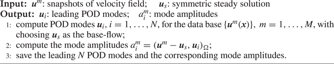
The computational cost for the cluster analysis can be significantly reduced in the POD subspace (Kaiser et al. Reference Kaiser, Noack, Cordier, Spohn, Segond, Abel, Daviller, Östh, Krajnović and Niven2014; Li et al. Reference Li, Fernex, Semaan, Tan, Morzyński and Noack2021), thus enabling an accurate compressed sensing of the original datasets. The centroids of the velocity field based on the POD mode amplitudes now read:
 \begin{equation} \boldsymbol{c}_{k} = \boldsymbol{u}_s + \frac{1}{n_k} \sum_{m=1}^M \chi_{k}^{m} \sum_{i=1}^{N} a_i^m\boldsymbol{u}_i. \end{equation}
We note that this POD process is just an option for data compression to speed up the clustering process, which can approximate the data distribution in a POD subspace with high accuracy. We can even apply the cluster-based approach to a feature-based subspace of the flow data, as Nair et al. (Reference Nair, Yeh, Kaiser, Noack, Brunton and Taira2019) who applied CROM to a three-dimensional phase space of the drag and lift forces.
In contrast to the nonlinear reconstruction of flows using a POD basis, the cluster-based approach neither decomposes the flow field nor extracts the dominant structures with the most fluctuating energies. Instead, it gathers similar snapshots and represents them with a linear combination of snapshots within the cluster. This combination is always in the original data space and there is no projection comparing with a POD model. In addition, the modelling process of the cluster-based method is automated based on the data topology in the state space, which is even suitable for multiple invariant sets. The differences between the cluster-based methods and the POD-based model have been discussed in Kaiser et al. (Reference Kaiser, Noack, Cordier, Spohn, Segond, Abel, Daviller, Östh, Krajnović and Niven2014), Li et al. (Reference Li, Fernex, Semaan, Tan, Morzyński and Noack2021). As an extension, the HiCNM strategy provides a multiscale solution for describing complex flow with transient dynamics.
Appendix D. Stochastic model for the asymptotic regime
In § 4, we have applied HiCNMs for the identification and analysis of complex dynamics with multiple scales and multiple invariant sets. The centroids and cluster index provide a concise representation of the original data set, and we can reconstruct the flow based on the time evolution of the cluster index. From the cluster analysis, we use a transition matrix to statistically record the possible motions between clusters, which can be used to predict the evolution of the cluster index. Hence, the dynamics reconstruction can also come from the stochastic model based on the transition matrix.
For a single trajectory, the transient dynamics is fully predictable and converges to the asymptotic dynamics. A stochastic model for the transient dynamics is not suggested because the clustering result may suffer from the multiscale problem, and some random walks will be mistakenly introduced into the transition matrix, like the destabilizing stage from the steady solution. In contrast, if there is no multiscale problem, all the transition probabilities should be 1 due to the predictable transient dynamics. Hence, there is no need to build the dynamics from a stochastic model and to discuss the probability distribution.
The asymptotic limit cycle at  $Re=80$ and torus at $Re=105$ are also fully predictable as there is no random walk. Only for the chaotic dynamics in the asymptotic regime at $Re=130$, can the transition matrix be used to construct a stochastic model. According to the current state in one of the clusters, it will choose the next destination according to the probability of transitions. Based on the local dynamics for the chaotic state in the group of clusters $\mathcal {C}_{k_1}, k_1 = 4, \ldots, 7$, the reconstructed dynamics and the probability distribution provided by the stochastic model are shown in figure 32. The main cycle $\mathcal {C}_1 \rightarrow \cdots \rightarrow \mathcal {C}_{6} \rightarrow \mathcal {C}_1$ and the random walks to $\mathcal {C}_{k_2}, k_2 = 7, \ldots, 10$ have been fairly reproduced, with the appropriate probability distribution.

Figure 32. Time evolution of the cluster index: the reconstructed dynamics (red curve) with the same initial cluster of the original dynamics (grey curve with coloured markers) for  $m_2=1, \ldots,8720$ (a); and probability distribution of all $m_2$ in figure 27 by a stochastic model using the transition matrix (b), at $Re=130$.


 Open access