


1. Introduction
The fluid–structure interaction (FSI) of a fluid current with a two-dimensional (2-D) thin foil or plate with chordwise flexibility has been extensively investigated theoretically, numerically and experimentally as a simple model to understand the propulsion mechanisms and performance of flapping appendages of natural fliers and swimmers, as well as their use to efficiently propel bioinspired aquatic and aerial robots (see, e.g. Shyy et al. (Reference Shyy, Aono, Chimakurthi, Trizila, Kang, Cesnik and Liu2010), Smits (Reference Smits2019) and Wu et al. (Reference Wu, Zhang, Tian, Li and Lu2020) for comprehensive reviews). Within the vast literature on the subject, the present work is focused on the role that resonances play in improving propulsion performance, contributing to the field with a new theoretically based analytical model to try to shed new light on the subject.
Theoretical approximations based on the 2-D linearized inviscid flow theory coupled to the Euler–Bernoulli (E–B) beam equation, although limited to small deformations of the foil and high Reynolds numbers, have proved to be very useful to facilitate the understanding of many relevant aspects of this complex FSI problem, helping to elucidate the mechanisms for the high efficiency obtainable by such propulsion systems. This approach, first used by Wu (Reference Wu1971 Reference Wub), and then by Katz & Weihs (Reference Katz and Weihs1978) for large amplitude oscillation of the foil, has been followed by a number of investigators (Alben Reference Alben2008; Michelin & Llewellyn Smith Reference Michelin and Llewellyn Smith2009; Alben et al. Reference Alben, Witt, Baker, Anderson and Lauder2012; Quinn et al. Reference Quinn, Lauder and Smits2014, Reference Quinn, Lauder and Smits2015; Moore Reference Moore2014; Paraz, Schouveiler & Eloy Reference Paraz, Schouveiler and Eloy2016; Piñeirua et al. Reference Piñeirua, Thiria and Godoy-Diana2017; Floryan & Rowley Reference Floryan and Rowley2018 and others) to analyse the influence of the bending rigidity and inertia on the propulsion performance of 2-D flexible flapping foils. It has generally been found from these inviscid flow theories that flexibility produces greater thrust when actuated near a fluid–structure natural frequency, but less otherwise, with larger propulsive efficiency than that of a rigid foil over a broad range of stiffnesses and frequencies. However, when viscous flow with nonlinearities associated with flow separation are considered, numerical and experimental investigations show that optimal performance can be achieved outside of the structural resonance conditions (Thiria & Godoy-Diana Reference Thiria and Godoy-Diana2010; Ramananarivo, Godoy-Diana & Thiria Reference Ramananarivo, Godoy-Diana and Thiria2011; Dewey et al. Reference Dewey, Boschitsch, Moored, Stone and Smits2013; Olivier & Dumas Reference Olivier and Dumas2016; Goza, Floryan & Rowley Reference Goza, Floryan and Rowley2020; D’Adamo et al. Reference D’Adamo, Collaud, Sosa and Godoy-Diana2022), but structural resonance always playing a relevant role in enhancing the propulsion performance for sufficiently small mass ratios of the foil (Zhang, Zhou & Luo Reference Zhang, Zhou and Luo2017).
Although linear inviscid theories represent a very significant simplification in relation to numerical simulations of the full FSI problem, and their results have provided very relevant advances in this field, they still require a considerable amount of numerical work, typically decomposing the displacement of the foil and the fluid motion into a Chebyshev series with a large number (infinite in theory) of parameters which have to be obtained numerically to capture the multiple resonant modes (e.g. Alben Reference Alben2009; Michelin & Llewellyn Smith Reference Michelin and Llewellyn Smith2009; Moore Reference Moore2017; Floryan & Rowley Reference Floryan and Rowley2018; Anevlavi et al. Reference Anevlavi, Filippas, Karperaki and Belibassakis2020; Mavroyiakoumou & Alben Reference Mavroyiakoumou and Alben2021). Analytical solutions for the FSI of flexible flapping foils, which may be obtained with additional simplifications within the same framework of the linear inviscid theories and the E–B beam equation, are undoubtedly very helpful in understanding the propulsive performance of flying and swimming animals, as well as for the preliminary design and improvement of bioinspired flying and swimming robotic models. For example, the interesting analytical approach by Moore (Reference Moore2014), who considered the particular case of a rigid foil with a prescribed heaving displacement and a passive pitching motion about its leading edge, relating the finite torsional stiffness of the leading edge with the kinematics of the rigid pitching motion and, hence, with the propulsive performance of the foil. A similar analytical model for a heaving foil was considered by Kodaly & Kang (Reference Kodaly and Kang2016), but for passive pitching associated with the flexibility of the foil rather than to its elastic support at the leading edge. More recently, Du & Wu (Reference Du and Wu2024) obtained simple analytical expressions that help to interpret the effect of the flexibility and regulate the propulsive performance of the flexible foil when only pitching is considered. A more general analytical approach for pitching and heaving flexible foils was considered by Fernandez-Feria & Alaminos-Quesada (Reference Fernandez-Feria and Alaminos-Quesada2021), where the foil passive deformation was modelled by a quartic polynomial approximation, reproducing previous numerical inviscid results up to the first resonant frequency of the system.
In the present work, the formulation in Fernandez-Feria & Alaminos-Quesada (Reference Fernandez-Feria and Alaminos-Quesada2021) is extended to cover consistently actuating frequencies up to the second resonance of the system by using a fifth-order polynomial approximation satisfying the boundary conditions at the leading and trailing edges of a general pitching and heaving flexible foil. This approach thus covers up to the frontier between the purely oscillatory behaviour and the undulatory behaviour of a 2-D flexible foil, for which analytical results from the E–B equation are no longer feasible due to the difficulty of satisfying the free-end boundary conditions at the trailing edge for prescribed leading edge conditions using simple undulatory approximations of the foil. Although the present approach sometimes yields trailing-edge deformation amplitudes at the second resonance of the system that are outside the validity limit of the linear theory, it is known that this behaviour can be easily corrected using a nonlinear transverse damping term in the E–B equation (e.g. Eloy, Kofman & Schouveiler Reference Eloy, Kofman and Schouveiler2012; Paraz et al. Reference Paraz, Schouveiler and Eloy2016), so that the results remain within the linear framework, showing a good agreement with experimental data on the deformation of flexible oscillating foils. Therefore, with this corrected deformation one may obtain the thrust, power and propulsive efficiency of the foil using the analytical expressions, also derived in the present work, from the linearized inviscid flow theory coupled with the E–B equation for a pitching and heaving foil whose deformation is given by a general fifth-order polynomial satisfying the boundary conditions.
As indicated in the abstract, this work is also intended to give a more systematic account of the analytic derivation of the lift, moment and the different flexural moments exerted by the inviscid fluid on a general flexible foil configuration. These are needed to derive the new expressions for the analytical approximation of the FSI through the successive moments of the E–B beam equation, containing the new contributions that allow us to capture both the first and the second resonance of the system. Similarly it is done for the thrust and power, with a more compact derivation that integrates the new contributions of the flexible foil into the circulatory and added mass terms in a way easier to use and to understand than in previous works. Obviously, many of these expressions contain common terms with some of these previous works (especially, Fernandez-Feria & Alaminos-Quesada (Reference Fernandez-Feria and Alaminos-Quesada2021)). But for the analytical formulation to be intelligible the new contributions cannot be presented in isolation, but within the complete expressions, which are written here. This is even more necessary due to the more systematic, and therefore partially different derivations, used here. Details about these differences are given throughout their derivations.
The paper is organized as follows. The problem is formulated in § 2, where it is also corroborated that the analytical approximate solution of the E–B equation recovers almost exactly the first two resonant frequencies of the system in vacuum. Section 3 presents the derivation of the lift, moment and the different flexural moments using a formulation based on the pressure difference in terms of the vorticity distribution, closing the new analytical approximation of the FSI of the system. Section 4 presents some flexural deformation results and their validation with experimental data after a nonlinear damping correction through a transverse drag coefficient. With this passive deformation, the thrust force can then be obtained with the new analytical expression derived in § 5 from the linearized vortex impulse theory for the pitching and heaving flexible foil with the general deformation considered in the present work. The input power and, therefore, the propulsive efficiency can finally be obtained through the first two moments of the E–B beam equation, whose analytical expressions are also given in § 5 along with a comparison with available experimental data on deformation, thrust, power and efficiency of small-amplitude heaving foils. All these expressions are used in § 6 to characterize and compare the propulsive performance of heaving and pitching flexible foils when actuated around the first and second natural modes. Finally, the conclusions are presented in § 7.
2. Formulation of the problem
The interaction of a uniform fluid current of velocity $U$
with a 2-D pitching and heaving flexible foil of chord length
$U$
with a 2-D pitching and heaving flexible foil of chord length $c$
and thickness
$c$
and thickness $\varepsilon$
is considered. For a thin plate,
$\varepsilon$
is considered. For a thin plate, $\varepsilon \ll c$
, one may use the 2-D E–B beam equation (e.g. Doyle Reference Doyle2001), which for an approximately inextensible plate with small amplitude of the heaving, pitching and flexural deformation in relation to its chord length and in the inviscid flow limit can be written as
$\varepsilon \ll c$
, one may use the 2-D E–B beam equation (e.g. Doyle Reference Doyle2001), which for an approximately inextensible plate with small amplitude of the heaving, pitching and flexural deformation in relation to its chord length and in the inviscid flow limit can be written as
 \begin{equation} \rho _s \varepsilon \frac {\partial ^2 z_s}{\partial t^2} + \frac {\partial ^2 }{\partial x^2} \left ( EI \frac {\partial ^2 z_s}{\partial x^2} \right) = \Delta p + F_{pz} \delta (x-x_p) - g \delta ^{\prime}(x-x_p) , \end{equation}
where (see figure 1) $z$
is the coordinate perpendicular to the plate at rest,
$z$
is the coordinate perpendicular to the plate at rest, $x$
is the coordinate along the uniform free stream, both coordinates centred at the midchord length of the plate,
$x$
is the coordinate along the uniform free stream, both coordinates centred at the midchord length of the plate, $z_s(x,t)$
is the displacement of the plate centreline in the
$z_s(x,t)$
is the displacement of the plate centreline in the $z\hbox{-}$
direction, satisfying
$z\hbox{-}$
direction, satisfying $|z_s| \ll c$
,
$|z_s| \ll c$
, $\rho _s$
is the solid density and
$\rho _s$
is the solid density and $E I= E \varepsilon ^3/12$
is the structural bending rigidity per unit span. On the right-hand side,
$E I= E \varepsilon ^3/12$
is the structural bending rigidity per unit span. On the right-hand side, $\Delta p = p^- - p^+$
is the fluid pressure difference between the lower and upper sides of the foil, whereas
$\Delta p = p^- - p^+$
is the fluid pressure difference between the lower and upper sides of the foil, whereas $F_{pz}$
and
$F_{pz}$
and $g$
stand for any additional point force and point moment (per unit span) acting at the pivot axis
$g$
stand for any additional point force and point moment (per unit span) acting at the pivot axis $x=x_p$
(e.g. to generate the heave and pitch motions of the foil, or exerted by springs and dampers for passive heave and pitch about the pivot axis).
$x=x_p$
(e.g. to generate the heave and pitch motions of the foil, or exerted by springs and dampers for passive heave and pitch about the pivot axis).

In particular, the first four moments of that equation are used here (e.g. Fernandez-Feria (Reference Fernandez-Feria2023), (6)–(10) in the small-amplitude and inextensible ( $E \varepsilon /(\rho U^2 c) \gg 1$
) limit, plus an additional moment):
$E \varepsilon /(\rho U^2 c) \gg 1$
) limit, plus an additional moment):
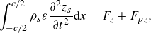 \begin{equation} \int _{-c/2}^{c/2} \rho _s \varepsilon \frac {\partial ^2 z_s}{\partial t^2} {\textrm d}x = F_z+F_{pz} , \end{equation}
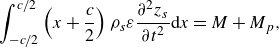 \begin{equation} \int _{-c/2}^{c/2} \left ( x + \frac {c}{2} \right) \rho _s \varepsilon \frac {\partial ^2 z_s}{\partial t^2} {\textrm d}x = M+M_{p} , \end{equation}
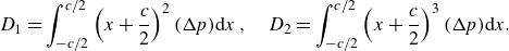
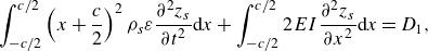 \begin{equation} \int _{-c/2}^{c/2} \left ( x + \frac {c}{2} \right)^2 \rho _s \varepsilon \frac {\partial ^2 z_s}{\partial t^2} {\textrm d}x + \int _{-c/2}^{c/2} 2 E I \frac {\partial ^2 z_s}{\partial x^2} {\textrm d} x= D_{1} , \end{equation}
 \begin{equation} \int _{-c/2}^{c/2} \left ( x + \frac {c}{2} \right)^3 \rho _s \varepsilon \frac {\partial ^2 z_s}{\partial t^2} {\textrm d}x + \int _{-c/2}^{c/2} 6 \left ( x + \frac {c}{2} \right) E I \frac {\partial ^2 z_s}{\partial x^2} {\textrm d} x= D_{2} . \end{equation}
In deriving these moment equations, free leading and trailing edges of the foil have been assumed, but with the pivot axis very close to the leading edge, so that the moments are approximately taken in relation to the point $x=x_p=-c/2$
. This selection is chosen for two main reasons: first, because thrust and efficiency are maximized when a pitching and heaving flexible foil is actuated at its leading edge (Moore Reference Moore2014, Reference Moore2015); second, because the analytical approximation for
$x=x_p=-c/2$
. This selection is chosen for two main reasons: first, because thrust and efficiency are maximized when a pitching and heaving flexible foil is actuated at its leading edge (Moore Reference Moore2014, Reference Moore2015); second, because the analytical approximation for $z_s(x,t)$
satisfying the leading and trailing edge constraints of the E–B beam equation is the simplest when the pivot axis is close to the leading edge (Fernandez-Feria Reference Fernandez-Feria2023). Linearized potential flow theory is assumed, with
$z_s(x,t)$
satisfying the leading and trailing edge constraints of the E–B beam equation is the simplest when the pivot axis is close to the leading edge (Fernandez-Feria Reference Fernandez-Feria2023). Linearized potential flow theory is assumed, with $F_z$
and
$F_z$
and $M$
the
$M$
the $z\hbox{-}$
component of the force (the lift) and the moment, respectively, exerted by the fluid flow on the foil,
$z\hbox{-}$
component of the force (the lift) and the moment, respectively, exerted by the fluid flow on the foil,
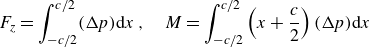 \begin{equation} F_z = \int _{-c/2}^{c/2} (\Delta p) {\textrm d}x \,, \quad M = \int _{-c/2}^{c/2} \left ( x + \frac {c}{2} \right) (\Delta p) {\textrm d}x \, \end{equation}
(note that $M$
is here positive when it is anticlockwise). Here
$M$
is here positive when it is anticlockwise). Here $D_1$
and
$D_1$
and $D_2$
are the first and second flexural deformation moments of the foil,
$D_2$
are the first and second flexural deformation moments of the foil,
 \begin{equation} D_1 = \int _{-c/2}^{c/2} \left ( x + \frac {c}{2} \right)^2 (\Delta p) {\textrm d}x \,, \quad D_2 = \int _{-c/2}^{c/2} \left ( x + \frac {c}{2} \right)^3 (\Delta p) {\textrm d}x . \end{equation}
Finally, $F_{pz}$
and
$F_{pz}$
and $M_p$
are, as commented on above, the point force and the point moment per unit span acting on the pivot axis.
$M_p$
are, as commented on above, the point force and the point moment per unit span acting on the pivot axis.
In relation to previous analytical models based on a linearized FSI theory (e.g. Moore Reference Moore2014; Kodaly & Kang Reference Kodaly and Kang2016; Fernandez-Feria & Alaminos-Quesada Reference Fernandez-Feria and Alaminos-Quesada2021; Du & Wu Reference Du and Wu2024), this is the only one which is based on a set of FSI equations that consistently considers the passive flexural deformation of the plate using two degrees of freedom through (2.4)–(2.5), thus covering a wider range of frequencies and stiffnesses, and for a general configuration of a pitching and heaving flexible plate.
2.1. Non-dimensional equations
The equations are non-dimensionalized using the fluid density $\rho$
, the free stream velocity
$\rho$
, the free stream velocity $U$
and the half-chord length
$U$
and the half-chord length $c/2$
. To simplify the notation, the same symbols are kept for the coordinates
$c/2$
. To simplify the notation, the same symbols are kept for the coordinates $(x,z)$
, the time
$(x,z)$
, the time $t$
(scaled with
$t$
(scaled with $2U/c$
) and the foil displacement
$2U/c$
) and the foil displacement $z_s$
. For
$z_s$
. For $z_s(x,t)$
to take into account the pitch and heave motions of the foil about the leading edge, as well as two flexural deformation degrees of freedom, at least a fifth-order polynomial must be used in
$z_s(x,t)$
to take into account the pitch and heave motions of the foil about the leading edge, as well as two flexural deformation degrees of freedom, at least a fifth-order polynomial must be used in $x$
, instead of the quartic one used in Fernandez-Feria & Alaminos-Quesada (Reference Fernandez-Feria and Alaminos-Quesada2021). Thus, imposing a pitch and heave motion at the leading edge (
$x$
, instead of the quartic one used in Fernandez-Feria & Alaminos-Quesada (Reference Fernandez-Feria and Alaminos-Quesada2021). Thus, imposing a pitch and heave motion at the leading edge ( $x=-1$
) and a free trailing edge (
$x=-1$
) and a free trailing edge ( $\partial ^2 z_s/\partial x^2 = \partial ^3 z_s/\partial x^3 =0$
at
$\partial ^2 z_s/\partial x^2 = \partial ^3 z_s/\partial x^3 =0$
at $x=1$
), this fifth-order polynomial approximation can be written as
$x=1$
), this fifth-order polynomial approximation can be written as
 \begin{align} z_s(x,t)&= h(t) - \alpha (t) (x+1) + d_1(t) [ 24(x+1)^2-8(x+1)^3+(x+1)^4] \nonumber \\ &\quad + d_2(t)[160(x+1)^2 -40(x+1)^3+(x+1)^5] \,, \quad \quad -1 \leqslant x \leqslant 1 , \end{align}
where $h(t)$
and
$h(t)$
and $\alpha (t)$
characterize the heave and pitch motions, respectively, and the unknown functions
$\alpha (t)$
characterize the heave and pitch motions, respectively, and the unknown functions $d_1(t)$
and
$d_1(t)$
and $d_2(t)$
characterize the flexural deformation. Note that the pitch angle
$d_2(t)$
characterize the flexural deformation. Note that the pitch angle $\alpha$
is positive when it is clockwise, as it is usual in airfoil aerodynamics, and that
$\alpha$
is positive when it is clockwise, as it is usual in airfoil aerodynamics, and that ${d}(t)$
in Fernandez-Feria & Alaminos-Quesada (Reference Fernandez-Feria and Alaminos-Quesada2021) is
${d}(t)$
in Fernandez-Feria & Alaminos-Quesada (Reference Fernandez-Feria and Alaminos-Quesada2021) is $24 d_1(t)$
here. The corresponding non-dimensional velocity of the foil’s centreline can be written as
$24 d_1(t)$
here. The corresponding non-dimensional velocity of the foil’s centreline can be written as
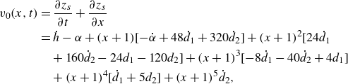 \begin{align} v_0(x,t)&= \frac {\partial z_s}{\partial t}+ \frac {\partial z_s}{\partial x}\nonumber \\ &= \dot {h} - \alpha + (x+1) [- \dot {\alpha } + 48 \dot {d}_1+320 \dot {d}_2] + (x+1)^2 [24 \dot {d}_1 \nonumber \\ &\quad +160 \dot {d}_2-24 d_1-120 d_2]+(x+1)^3 [-8 \dot {d}_1-40 \dot {d}_2+4 d_1] \\ &\quad +(x+1)^4 [\dot {d}_1+5 d_2] + (x+1)^5 \dot {d}_2 , \nonumber \end{align}
where dots are used for the derivatives with respect to the non-dimensional time $t$
.
$t$
.
Assuming that $\rho _s$
,
$\rho _s$
, $\varepsilon$
and
$\varepsilon$
and $E$
are constant along the foil’s chord length, the non-dimensional counterparts of (2.2)–(2.5) can be written as
$E$
are constant along the foil’s chord length, the non-dimensional counterparts of (2.2)–(2.5) can be written as
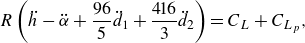 \begin{equation} R \left ( \ddot {h} - \ddot {\alpha } + \frac {96}{5} \ddot {d}_1 + \frac {416}{3} \ddot {d}_2 \right) =C_L+C_{L_p} , \end{equation}
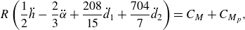 \begin{equation} R \left ( \frac {1}{2} \ddot {h} - \frac {2}{3} \ddot {\alpha } + \frac {208}{15} \ddot {d}_1 + \frac {704}{7} \ddot {d}_2 \right) =C_M+C_{M_p} , \end{equation}
 \begin{equation} R \left ( \frac {4}{3} \ddot {h} - 2 \ddot {\alpha } + \frac {4544}{105} \ddot {d}_1 + \frac {944}{3} \ddot {d}_2 \right) + S \left ( \frac {32}{3} d_1 + 80 d_2 \right) = C_{F_1} , \end{equation}
 \begin{equation} R \left ( 2 \ddot {h} - \frac {16}{5} \ddot {\alpha } + \frac {496}{7} \ddot {d}_1 + \frac {32 512}{63} \ddot {d}_2 \right) + S \left ( 16 d_1 + 128 d_2 \right) = C_{F_2} , \end{equation}
where the non-dimensional parameters
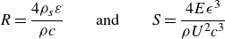 \begin{equation} R = \frac {4 \rho _s \varepsilon }{\rho c} \quad \quad \text{and} \quad \quad S= \frac {4 E \epsilon ^3}{\rho U^2 c^3} \end{equation}
are the mass ratio (or inertia parameter) and the bending stiffness parameter, respectively, and the following fluid force and moment coefficients have been defined:
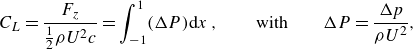 \begin{equation} C_L = \frac {F_z}{\frac {1}{2} \rho U^2 c} = \int _{-1}^1 (\Delta P) {\textrm d} x \,, \quad \quad \text{with} \quad \quad \Delta P = \frac {\Delta p}{\rho U^2} , \end{equation}
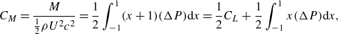 \begin{equation} C_M = \frac {M}{\frac {1}{2} \rho U^2 c^2} = \frac {1}{2} \int _{-1}^1 (x+1) (\Delta P) {\textrm d} x = \frac {1}{2} C_L + \frac {1}{2} \int _{-1}^1 x (\Delta P) {\textrm d} x , \end{equation}
 \begin{equation} C_{F_1} = \frac {D_1}{\rho U^2 \left ( \frac {c}{2} \right)^3} = \int _{-1}^1 (x+1)^2 (\Delta P) {\textrm d} x = - C_L + 4 C_M + \int _{-1}^1 x^2 (\Delta P) {\textrm d} x , \end{equation}
 \begin{equation} C_{F_2} = \frac {D_2}{\rho U^2 \left ( \frac {c}{2} \right)^4} = \int _{-1}^1 (x+1)^3 (\Delta P) {\textrm d} x = C_L - 6 C_M + 3 C_{F_1} + \int _{-1}^1 x^3 (\Delta P) {\textrm d} x \,; \end{equation}
together with the point force and moment coefficients,
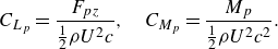 \begin{equation} C_{L_p} = \frac {F_{pz}}{\frac {1}{2} \rho U^2 c} , \quad C_{M_p} = \frac {M_p}{\frac {1}{2} \rho U^2 c^2} . \end{equation}
The above expressions of the fluid coefficients are written in terms of the non-dimensional pressure difference $\Delta P=(p^-p^+)/(\rho U^2)$
to facilitate their computation in terms of
$\Delta P=(p^-p^+)/(\rho U^2)$
to facilitate their computation in terms of $h(t)$
,
$h(t)$
, $\alpha (t)$
,
$\alpha (t)$
, $d_1(t)$
and
$d_1(t)$
and $d_2(t)$
, and their derivatives (see § 3). Although the expressions for the coefficients will be obtained for any temporal variation of these functions, a general harmonic motion of the plate with frequency
$d_2(t)$
, and their derivatives (see § 3). Although the expressions for the coefficients will be obtained for any temporal variation of these functions, a general harmonic motion of the plate with frequency $\omega$
will be considered in the computations; i.e. the real parts (say) of
$\omega$
will be considered in the computations; i.e. the real parts (say) of
 \begin{equation} h(t)= h_0 e^{i k t} \,, \quad \alpha (t)= \alpha _0 e^{ikt} \, \quad {\textrm{with}} \quad \alpha _0= a_0 e^{i \phi } , \end{equation}
 \begin{equation} d_1(t)= d_{10} e^{i k t}, \quad d_2(t)= d_{20} e^{ikt}, \quad {\textrm{with}} \quad d_{10}= d_{1m} e^{i \psi _1}, \quad d_{20}= d_{2m} e^{i \psi _2} , \end{equation}
where $h_0$
and
$h_0$
and $a_0$
are the heave and pitch amplitudes,
$a_0$
are the heave and pitch amplitudes, $d_{1m}$
and
$d_{1m}$
and $d_{2m}$
the amplitudes of the first and second flexural deflection modes, and the heave phase is taken zero as usual, so that
$d_{2m}$
the amplitudes of the first and second flexural deflection modes, and the heave phase is taken zero as usual, so that $\phi$
,
$\phi$
, $\psi _1$
and
$\psi _1$
and $\psi _2$
are the phase shifts of pitch and the two deflection modes, respectively, in relation to the heave phase. Finally,
$\psi _2$
are the phase shifts of pitch and the two deflection modes, respectively, in relation to the heave phase. Finally,
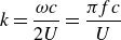 \begin{equation} k= \frac {\omega c}{2 U} = \frac {\pi f c}{U} \end{equation}
is the non-dimensional, or reduced, frequency.
2.2. Validation of the FSI model with the first two natural frequencies in vacuum
Before deriving the fluid coefficients $C_L, C_M, C_{F_1}$
and
$C_L, C_M, C_{F_1}$
and $C_{F_2}$
, it is shown here that the above formulation with the fifth-order polynomial approximation (2.8) for
$C_{F_2}$
, it is shown here that the above formulation with the fifth-order polynomial approximation (2.8) for $z_s$
captures very accurately the first two natural frequencies of the foil in vacuum.
$z_s$
captures very accurately the first two natural frequencies of the foil in vacuum.
Substituting (2.20)–(2.21) into the moment equations (2.12) and (2.13) with $C_{F_1}=C_{F_2}=0$
, i.e. in absence of fluid–foil interaction, one obtains the following linear equation for the two deflection amplitudes
$C_{F_1}=C_{F_2}=0$
, i.e. in absence of fluid–foil interaction, one obtains the following linear equation for the two deflection amplitudes $d_{10}$
and
$d_{10}$
and $d_{20}$
in terms of the pitch and heave amplitudes,
$d_{20}$
in terms of the pitch and heave amplitudes, $\alpha _0$
and
$\alpha _0$
and $h_0$
, the structural parameters and the frequency
$h_0$
, the structural parameters and the frequency $k$
:
$k$
:
 \begin{equation} { \mathsf{A}}_0 \cdot {\boldsymbol {d}}_0 = {\boldsymbol {b}}_0 , \end{equation}
with
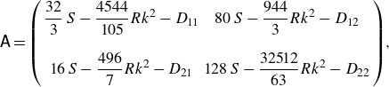
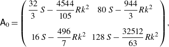 \begin{equation} { \mathsf{A}}_0 = \left ( \begin{array}{cc} \displaystyle \frac {32}{3} \, S - \displaystyle \frac {4544}{105} R k^2 & 80 \, S - \displaystyle \frac {944}{3} R k^2 \\ \\ 16 \, S - \displaystyle \frac {496}{7} R k^2 & 128 \, S - \displaystyle \frac {32512}{63} R k^2 \end{array} \right)\!, \end{equation}
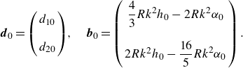 \begin{equation} {\boldsymbol {d}}_0 = \left ( \begin{array}{c} d_{10} \\ \\ d_{20} \end{array} \right)\!, \quad {\boldsymbol {b}}_0 = \left ( \begin{array}{c} \displaystyle \frac {4}{3} R k^2 h_0 - 2 R k^2 \alpha _0 \\ \\ 2 R k^2 h_0 - \displaystyle \frac {16}{5} R k^2 \alpha _{0} \end{array} \right) . \end{equation}
The resonant frequencies, or frequencies where the flexural deformation amplitudes $d_{10}$
and
$d_{10}$
and $d_{20}$
diverge, are obtained from det
$d_{20}$
diverge, are obtained from det $({ \mathsf{A}}_0)=0$
, yielding the first two resonant frequencies in vacuum as the two real positive roots of that equation,
$({ \mathsf{A}}_0)=0$
, yielding the first two resonant frequencies in vacuum as the two real positive roots of that equation,
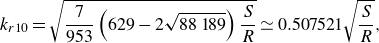 \begin{equation} k_{r10}= \sqrt {\frac {7}{953} \left ( 629 -2 \sqrt {88\,189} \right) \frac {S}{R} } \simeq 0.507521 \sqrt {\frac {S}{R} } , \end{equation}
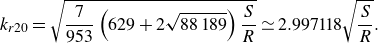 \begin{equation} k_{r20}= \sqrt {\frac {7}{953} \left ( 629 +2 \sqrt {88\,189} \right) \frac {S}{R} } \simeq 2.997118 \sqrt {\frac {S}{R} } . \end{equation}
These values are in very good agreement with the exact results for the first two resonant frequencies of a beam clamped at the leading edge (e.g. Timoshenko, Young & Weaver Reference Timoshenko, Young and Weaver1974, § 5.11): $\omega _{i} = \lambda _i^2 \sqrt {E \varepsilon ^2 /(12 \rho _s \varepsilon c^4)}$
, with
$\omega _{i} = \lambda _i^2 \sqrt {E \varepsilon ^2 /(12 \rho _s \varepsilon c^4)}$
, with $\lambda _1=1.87510$
and
$\lambda _1=1.87510$
and $\lambda _2=4.69409$
, which in the present non-dimensional notation are
$\lambda _2=4.69409$
, which in the present non-dimensional notation are $k_1=0.507491 \sqrt {S/R}$
and
$k_1=0.507491 \sqrt {S/R}$
and $k_2=3.180403 \sqrt {S/R}$
(relative errors with (2.26) and (2.27) of
$k_2=3.180403 \sqrt {S/R}$
(relative errors with (2.26) and (2.27) of $0.006 \, \%$
and
$0.006 \, \%$
and $5.7 \, \%$
, respectively). Thus, (2.8) is the simplest model for the chordwise deformation of a pitching and heaving flexible plate covering the first two resonant natural modes.
$5.7 \, \%$
, respectively). Thus, (2.8) is the simplest model for the chordwise deformation of a pitching and heaving flexible plate covering the first two resonant natural modes.
3. Fluid force and moment coefficients
To obtain $C_L, C_M, C_{F_1}$
and
$C_L, C_M, C_{F_1}$
and $C_{F_2}$
in a systematic way from (2.15) to (2.18) it is convenient to write the non-dimensional pressure difference
$C_{F_2}$
in a systematic way from (2.15) to (2.18) it is convenient to write the non-dimensional pressure difference $\Delta P$
in terms of the non-dimensional vorticity density distribution on the plate. In a linearized theory it is assumed that vorticity is concentrated along the
$\Delta P$
in terms of the non-dimensional vorticity density distribution on the plate. In a linearized theory it is assumed that vorticity is concentrated along the $x\hbox{-}$
axis, both on the plate surface and its trailing wake (e.g. Newman (Reference Newman1977), chapter 5). On the surface of the plate, the non-dimensional vorticity density distribution is
$x\hbox{-}$
axis, both on the plate surface and its trailing wake (e.g. Newman (Reference Newman1977), chapter 5). On the surface of the plate, the non-dimensional vorticity density distribution is $\varpi _s(x,t) = u^+ - u^-$
, where
$\varpi _s(x,t) = u^+ - u^-$
, where $u^+$
and
$u^+$
and $u^-$
are the non-dimensional fluid velocity on the upper and lower sides of the plate, respectively. Using the unsteady, linearized Bernoulli equation the non-dimensional pressure difference can be written as (see Appendix A)
$u^-$
are the non-dimensional fluid velocity on the upper and lower sides of the plate, respectively. Using the unsteady, linearized Bernoulli equation the non-dimensional pressure difference can be written as (see Appendix A)
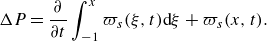 \begin{equation} \Delta P = \frac {\partial }{\partial t} \int _{-1}^x \varpi _s(\xi,t) {\textrm d}\xi + \varpi _s(x,t) . \end{equation}
The $n$
th moment of
$n$
th moment of $\Delta P$
, appearing in (2.15)–(2.18) for
$\Delta P$
, appearing in (2.15)–(2.18) for $n= 0,1,2$
and
$n= 0,1,2$
and $3$
, can then be expressed, after integrating by parts, as
$3$
, can then be expressed, after integrating by parts, as
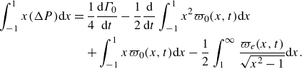
 \begin{equation} \int _{-1}^1 x^n (\Delta P) {\textrm d}x = \frac {\textrm d}{{\textrm d}t} \int _{-1}^1 \frac {1-x^{n+1}}{n+1} \varpi _s(x,t) {\textrm d}x + \int _{-1}^1 x^n \varpi _s(x,t) {\textrm d} x . \end{equation}
Following von Kármán & Sears (Reference von Kármán and Sears1938), the vorticity distribution on the foil can be decomposed as
 \begin{equation} \varpi _s(x,t) = \varpi _0(x,t)+\varpi _{se}(x,t) , \end{equation}
where $\varpi _0$
is the contribution from the motion of the foil (2.9) through the integral equation (see, e.g. Newman (Reference Newman1977), § 5.15)
$\varpi _0$
is the contribution from the motion of the foil (2.9) through the integral equation (see, e.g. Newman (Reference Newman1977), § 5.15)
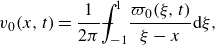 \begin{equation} v_{0}(x,t)= \frac {1}{2\pi } {\int \!\!\!\!\!\!-}_{\!\!-1}^{1}\frac {\varpi _{0}(\xi,t)}{\xi -x}{\textrm d}\xi , \end{equation}
with $\int \!\!\!\!\!-$
denoting Cauchy’s principal value of the integral, whereas
$\int \!\!\!\!\!-$
denoting Cauchy’s principal value of the integral, whereas $\varpi _{se}$
is the contribution from the wake vorticity
$\varpi _{se}$
is the contribution from the wake vorticity $\varpi _e(x,t)$
, which in the long time extends to infinity in first approximation,
$\varpi _e(x,t)$
, which in the long time extends to infinity in first approximation, $1 \leqslant x \lt \infty$
, and is given by von Kármán & Sears (Reference von Kármán and Sears1938), (7), as
$1 \leqslant x \lt \infty$
, and is given by von Kármán & Sears (Reference von Kármán and Sears1938), (7), as
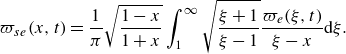 \begin{equation} \varpi _{se}(x,t)=\frac {1}{\pi }\sqrt {\frac {1-x}{1+x}}\int _1^{\infty }\sqrt {\frac {\xi +1}{\xi -1}}\frac {\varpi _{e}(\xi,t)}{\xi -x}{\textrm d}\xi . \end{equation}
The solution of (3.4) yields
 \begin{equation} \varpi _{0}(x,t) = \frac {2}{\pi \sqrt {1-x^2}}\left [ -\frac {2}{\pi }{\int \!\!\!\!\!\!-}_{\!\!-1}^{1}\frac {\sqrt {1-\xi ^2}}{\xi -x} v_0(\xi,t) {\textrm d}\xi + \frac {\Gamma _0(t)}{2} \right]\!, \end{equation}
with
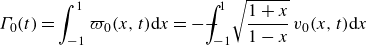 \begin{equation} \Gamma _0(t)= \int _{-1}^1 \varpi _0(x,t) {\textrm d} x = - {\int \!\!\!\!\!\!-}_{\!\!-1}^1 \sqrt {\frac {1+x}{1-x}} \, v_0(x,t) {\textrm d}x \end{equation}
the quasisteady bound circulation around the foil (i.e. without considering the effect of the unsteady wake). From Kelvin’s circulation theorem these vorticity distributions are related to each other through
 \begin{equation} \int _{-1}^1 \varpi _{s}(x,t) {\textrm d} x + \int _1^\infty \varpi _e(x,t) {\textrm d}x = \Gamma _0(t) + \int _{1}^\infty \sqrt {\frac {x+1}{x-1}}\, \varpi _{e}(x,t) {\textrm d} x = 0 , \end{equation}
where use has been made of (3.3) and (3.5) for the integral of $\varpi _{se}$
and the definition (3.7) of
$\varpi _{se}$
and the definition (3.7) of $\Gamma _0$
.
$\Gamma _0$
.
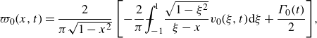
3.1. Lift coefficient
According to (2.15) and (3.2), the lift coefficient can be obtained from
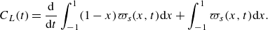 \begin{equation} C_L(t)= \frac {\textrm d}{{\textrm d}t} \int _{-1}^1 (1-x) \varpi _s(x,t) {\textrm d}x + \int _{-1}^1 \varpi _s(x,t) {\textrm d} x . \end{equation}
After using Kelvin’s theorem (3.8), integrating by parts and performing the integral $\int _{-1}^1 x \varpi _{se} {\textrm d}x$
using (3.5), this can be written as (von Kármán & Sears Reference von Kármán and Sears1938)
$\int _{-1}^1 x \varpi _{se} {\textrm d}x$
using (3.5), this can be written as (von Kármán & Sears Reference von Kármán and Sears1938)
 \begin{equation} C_L(t) = - \frac {\textrm d}{{\textrm d}t} \int _{-1}^1 x \varpi _0(x,t) {\textrm d}x - \int _{1}^\infty \frac {x \, \varpi _e(x,t)}{\sqrt {x^2-1}} {\textrm d} x \equiv C_{L_0}(t) + C_{L_e} (t). \end{equation}
The first term, $C_{L_0}$
, is the added-mass or non-circulatory contribution to the lift, which can be readily obtained once
$C_{L_0}$
, is the added-mass or non-circulatory contribution to the lift, which can be readily obtained once $\varpi _0(x,t)$
is computed from (3.6) using (2.9):
$\varpi _0(x,t)$
is computed from (3.6) using (2.9):
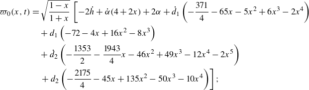 \begin{align} \varpi _0(x,t) &= \sqrt {\frac {1 - x}{1 + x}} \, \left [ - 2 \dot {h} + \dot {\alpha } (4+2x)+2 \alpha + \dot {d}_1 \left ( - \frac {371}{4} -65 x - 5 x^2 + 6 x^3 - 2 x^4 \right) \right.\nonumber \\ &\quad + d_1\left ( -72 - 4 x + 16 x^2 - 8 x^3 \right) \nonumber \\ &\quad + \dot {d}_2 \left ( - \frac {1353}{2} - \frac {1943}{4} x - 46 x^2 + 49 x^3-12x^4-2 x^5 \right)\nonumber \\ &\quad \left. + \,d_2 \left ( - \frac {2175}{4} -45 x +135 x^2-50 x^3- 10 x^4 \right) \right] ; \end{align}
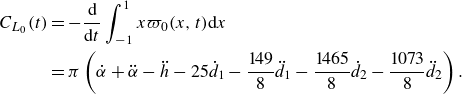 \begin{align} C_{L_0}(t)& = - \frac {\textrm d}{{\textrm d}t} \int _{-1}^1 x \varpi _0(x,t) {\textrm d}x \nonumber \\ &= \pi \left ( \dot {\alpha } + \ddot {\alpha } - \ddot {h} - 25 \dot {d}_1 - \frac {149}{8} \ddot {d}_1 - \frac {1465}{8} \dot {d}_2 - \frac {1073}{8} \ddot {d}_2 \right) . \end{align}
Obviously, the contributions from the pitch and heave, $\alpha (t)$
and
$\alpha (t)$
and $h(t)$
, coincide with those obtained by Theodorsen (Reference Theodorsen1935) and von Kármán & Sears (Reference von Kármán and Sears1938), while the contribution from
$h(t)$
, coincide with those obtained by Theodorsen (Reference Theodorsen1935) and von Kármán & Sears (Reference von Kármán and Sears1938), while the contribution from $d_1(t)$
coincide with that obtained in Alaminos-Quesada & Fernandez-Feria (Reference Alaminos-Quesada and Fernandez-Feria2020) with
$d_1(t)$
coincide with that obtained in Alaminos-Quesada & Fernandez-Feria (Reference Alaminos-Quesada and Fernandez-Feria2020) with ${d}(t)=24 d_1(t)$
. Only the contributions from
${d}(t)=24 d_1(t)$
. Only the contributions from $d_2(t)$
, which captures the second natural frequency of the foil, is new here. Similarly it happens for all the other coefficients calculated in the rest of this section, except for
$d_2(t)$
, which captures the second natural frequency of the foil, is new here. Similarly it happens for all the other coefficients calculated in the rest of this section, except for $C_{F_2}$
, which is completely new, but their derivations are summarized here for completeness, and because the new contributions from
$C_{F_2}$
, which is completely new, but their derivations are summarized here for completeness, and because the new contributions from $d_2(t)$
have to be obtained together with the rest to be integrated into the new expressions derived here.
$d_2(t)$
have to be obtained together with the rest to be integrated into the new expressions derived here.
To compute the circulatory contribution $C_{L_c}$
, the wake vorticity distribution
$C_{L_c}$
, the wake vorticity distribution $\varpi _e$
is obtained from Kelvin’s theorem (3.8) assuming the harmonic motion (2.20)–(2.21) and taking into account that
$\varpi _e$
is obtained from Kelvin’s theorem (3.8) assuming the harmonic motion (2.20)–(2.21) and taking into account that $\varpi _e(x,t)=\varpi _e(X)$
, with
$\varpi _e(x,t)=\varpi _e(X)$
, with $X=x-t$
, so that, writing
$X=x-t$
, so that, writing $\Gamma _0(t)= G_0 e^{ikt}$
, it results that
$\Gamma _0(t)= G_0 e^{ikt}$
, it results that $\varpi _e(x,t)= g e^{i k (t-x)}$
with
$\varpi _e(x,t)= g e^{i k (t-x)}$
with $g= -G_0 / \int _1^\infty \sqrt {(x+1)/(x-1)} \, e^{- i k x} {\textrm d}x$
. Solving this integral in terms of the Hankel functions
$g= -G_0 / \int _1^\infty \sqrt {(x+1)/(x-1)} \, e^{- i k x} {\textrm d}x$
. Solving this integral in terms of the Hankel functions $H_0^{(2)} (k)$
and
$H_0^{(2)} (k)$
and $H_1^{(2)} (k)$
, and writing the result again in terms of
$H_1^{(2)} (k)$
, and writing the result again in terms of $\Gamma _0(t)$
, one gets (von Kármán & Sears Reference von Kármán and Sears1938)
$\Gamma _0(t)$
, one gets (von Kármán & Sears Reference von Kármán and Sears1938)
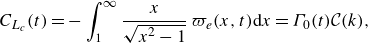 \begin{equation} C_{L_c}(t) = - \int _{1}^\infty \frac {x}{\sqrt {x^2-1}} \, \varpi _e(x,t) {\textrm d} x = \Gamma _0(t) \mathcal{C} (k) , \end{equation}
where
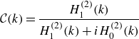 \begin{equation} \mathcal{C}(k)= \frac {H_1^{(2)} (k)}{H_1^{(2)} (k)+ i H_0^{(2)} (k)} \end{equation}
is Theodorsen’s function. This result coincides formally with Theodorsen (Reference Theodorsen1935) and von Kármán & Sears (Reference von Kármán and Sears1938), but now $\Gamma _0(t)$
contains more terms. It is obtained from (3.7) using (2.9):
$\Gamma _0(t)$
contains more terms. It is obtained from (3.7) using (2.9):
 \begin{equation} \Gamma _0(t)= \pi \left [ - 2 \dot {h} + 3 \dot {\alpha } + 2 \alpha - \frac {263}{4} \dot {d}_1 - 59 d_1 - \frac {3831}{8} \dot {d}_2 - \frac {1755}{4} d_2 \right] . \end{equation}
Note that although (3.13) has been derived for a harmonic motion, it can be extrapolated to more general foil motions using this expression for $\Gamma _0(t)$
, not restricted to a harmonic motion of the foil.
$\Gamma _0(t)$
, not restricted to a harmonic motion of the foil.
3.2. Moment coefficient
Once $C_L$
is obtained, to compute
$C_L$
is obtained, to compute $C_M$
from (2.16) it suffices to obtain
$C_M$
from (2.16) it suffices to obtain
 \begin{equation} \int _{-1}^1 x (\Delta P) {\textrm d}x = \frac {\textrm d}{{\textrm d}t} \int _{-1}^1 \frac {1-x^2}{2} \varpi _s(x,t) {\textrm d}x + \int _{-1}^1 x \varpi _s(x,t) {\textrm d} x . \end{equation}
Again, after some manipulations using Kelvin’s theorem (3.8), integration by parts, performing the integrals $\int _{-1}^1 x^2 \varpi _{se} {\textrm d}x$
and
$\int _{-1}^1 x^2 \varpi _{se} {\textrm d}x$
and $\int _{-1}^1 x \varpi _{se} {\textrm d}x$
using (3.5) and taking into account that
$\int _{-1}^1 x \varpi _{se} {\textrm d}x$
using (3.5) and taking into account that $d (\int _1^\infty A(x) \varpi _e(x-t) {\textrm d}x)/{\textrm d}t = \int _1^\infty A^{\prime}(x) \varpi _e(x-t) {\textrm d}x$
when
$d (\int _1^\infty A(x) \varpi _e(x-t) {\textrm d}x)/{\textrm d}t = \int _1^\infty A^{\prime}(x) \varpi _e(x-t) {\textrm d}x$
when $A(x=1)=0$
, one gets
$A(x=1)=0$
, one gets
 \begin{align} \int _{-1}^1 x (\Delta P) {\textrm d}x & = \frac {1}{4} \frac {{\textrm d} \Gamma _0}{{\textrm d}t} - \frac {1}{2} \frac {\textrm d}{{\textrm d}t} \int _{-1}^1 x^2 \varpi _0(x,t) {\textrm d}x\nonumber\\ &\quad + \int _{-1}^1 x \varpi _0(x,t) {\textrm d}x - \frac {1}{2} \int _1^\infty \frac {\varpi _e(x,t)}{\sqrt {x^2-1}} {\textrm d} x . \end{align}
Only the last term contributes to the circulatory moment. Combining this expression with $C_L$
in (2.16) and performing the integrals in a similar way to how it has been done for
$C_L$
in (2.16) and performing the integrals in a similar way to how it has been done for $C_L$
, the moment coefficient can be conveniently written as
$C_L$
, the moment coefficient can be conveniently written as
 \begin{equation} C_M(t)=C_{M_0}(t)+ C_{M_c}(t) , \end{equation}
with the added-mass term
 \begin{align} C_{M_0}(t)&= \frac {\pi }{256} \left ( 192 \dot {\alpha } + 144 \ddot {\alpha } - 128 \ddot {h} - 576 d_1 -5248 \dot {d}_1 - 2800 \ddot {d}_1 \right.\nonumber \\ & \quad \left. - 4640 d_2 - 38680 \dot {d}_2-20213 \ddot {d}_2 \right)\!, \end{align}
and
 \begin{equation} C_{M_c}(t)= \tfrac {1}{4} \Gamma _0 (t) \mathcal{C}(k) , \end{equation}
where $\Gamma _0(t)$
is given by (3.15) and
$\Gamma _0(t)$
is given by (3.15) and $\mathcal{C}(k)$
by (3.14).
$\mathcal{C}(k)$
by (3.14).
3.3. First flexural moment coefficient
According to (2.17), to obtain $C_{F_1}$
one needs the additional computation of
$C_{F_1}$
one needs the additional computation of
 \begin{equation} \int _{-1}^1 x^2 (\Delta P) {\textrm d}x = \frac {\textrm d}{{\textrm d}t} \int _{-1}^1 \frac {1-x^3}{3} \varpi _s(x,t) {\textrm d}x + \int _{-1}^1 x^2 \varpi _s(x,t) {\textrm d} x , \end{equation}
which after some lengthy manipulations can be written as
 \begin{align} \int _{-1}^1 x^2 (\Delta P) {\textrm d}x & = - \frac {1}{2} \Gamma _0 - \frac {1}{3} \frac {\textrm d}{{\textrm d}t} \int _{-1}^1 x^3 \varpi _0(x,t) {\textrm d}x \nonumber\\ & \quad + \int _{-1}^1 x^2 \varpi _0(x,t) {\textrm d}x - \frac {1}{2} \int _1^\infty \frac {x \varpi _e(x,t)}{\sqrt {x^2-1}} {\textrm d} x . \end{align}
Thus, performing the integrals and using the above expressions of $C_L$
and
$C_L$
and $C_M$
in (2.17), one gets
$C_M$
in (2.17), one gets
 \begin{equation} C_{F_1}(t)=C_{F_{10}}(t)+ C_{F_{1c}}(t) , \end{equation}
with
 \begin{align} C_{F_{10}}(t)&= \frac {\pi }{192} \left ( 384 \dot {\alpha } + 288 \ddot {\alpha } - 240 \ddot {h} - 1056 d_1 -10848 \dot {d}_1 - 5745 \ddot {d}_1 \right.\nonumber \\ & \quad \left. - 8640 d_2 - 80190 \dot {d}_2-41540 \ddot {d}_2 \right)\!, \end{align}
 \begin{equation} C_{F_{1c}}(t)= \tfrac {1}{2} \Gamma _0 (t) \mathcal{C}(k) . \end{equation}
Except for the new terms with $d_2(t)$
, this expression coincides with
$d_2(t)$
, this expression coincides with $C_F$
obtained in Fernandez-Feria & Alaminos-Quesada (Reference Fernandez-Feria and Alaminos-Quesada2021) by a slightly different approach, with
$C_F$
obtained in Fernandez-Feria & Alaminos-Quesada (Reference Fernandez-Feria and Alaminos-Quesada2021) by a slightly different approach, with $d(t)=24 d_1(t)$
in that reference.
$d(t)=24 d_1(t)$
in that reference.
3.4. Second flexural moment coefficient
Finally, to obtain $C_{F_2}$
one needs to compute
$C_{F_2}$
one needs to compute
 \begin{equation} \int _{-1}^1 x^3 (\Delta P) {\textrm d}x = \frac {\textrm d}{{\textrm d}t} \int _{-1}^1 \frac {1-x^4}{4} \varpi _s(x,t) {\textrm d}x + \int _{-1}^1 x^4 \varpi _s(x,t) {\textrm d} x , \end{equation}
which can be written as
 \begin{align} \int _{-1}^1 x^3 (\Delta P) {\textrm d}x & = \frac {3}{32} \frac {{\textrm d} \Gamma _0}{{\textrm d}t} - \frac {1}{4} \frac {\textrm d}{{\textrm d}t} \int _{-1}^1 x^4 \varpi _0(x,t) {\textrm d}x \nonumber\\ &\quad + \int _{-1}^1 x^3 \varpi _0(x,t) {\textrm d}x - \frac {3}{8} \int _1^\infty \frac {\varpi _e(x,t)}{\sqrt {x^2-1}} {\textrm d} x . \end{align}
Substituting into (2.18) and performing the integrals, the second flexural moment coefficient can be written as
 \begin{equation} C_{F_2}(t)=C_{F_{20}}(t)+ C_{F_{2c}}(t) , \end{equation}
with the added-mass term
 \begin{align} C_{F_{20}}(t)&= \frac {\pi }{128} \left ( 368 \dot {\alpha } + 280 \ddot {\alpha } - 224 \ddot {h} - 912 d_1 -10580 \dot {d}_1 - 5680 \ddot {d}_1 \right.\nonumber \\ & \quad \left. - 7530 d_2 - 78350 \dot {d}_2-41117 \ddot {d}_2 \right)\!, \end{align}
and the circulatory term
 \begin{equation} C_{F_{2c}}(t)= \frac {5}{8} \Gamma _0 (t) \mathcal{C}(k) , \end{equation}
where $\Gamma _0(t)$
is given by (3.15) and
$\Gamma _0(t)$
is given by (3.15) and $\mathcal{C}(k)$
by (3.14).
$\mathcal{C}(k)$
by (3.14).
4. Validation of flexural deformation
Once the necessary aerodynamic loads on the flexible plate have been calculated for $z_s$
given by (2.8), (2.10)–(2.13) are closed. In particular, with the expressions for
$z_s$
given by (2.8), (2.10)–(2.13) are closed. In particular, with the expressions for $C_{F_1}$
and
$C_{F_1}$
and $C_{F_2}$
one may solve (2.12)–(2.13) to obtain the passive flexural deformation of the plate, which is done in this section, before considering the propulsion problem in § 5.
$C_{F_2}$
one may solve (2.12)–(2.13) to obtain the passive flexural deformation of the plate, which is done in this section, before considering the propulsion problem in § 5.
For given pitching and heaving harmonic motions $h(t)$
and
$h(t)$
and $\alpha (t)$
, the corresponding flexural deformation functions
$\alpha (t)$
, the corresponding flexural deformation functions $d_1(t)$
and
$d_1(t)$
and $d_2(t)$
can be computed from (2.12) and (2.13) once the flexural coefficients
$d_2(t)$
can be computed from (2.12) and (2.13) once the flexural coefficients $C_{F_1}$
and
$C_{F_1}$
and $C_{F_2}$
obtained in §§ 3.3 and 3.4 are written in terms of the harmonic motion (2.20)–(2.21). Equations (2.12) and (2.13) can then be written as
$C_{F_2}$
obtained in §§ 3.3 and 3.4 are written in terms of the harmonic motion (2.20)–(2.21). Equations (2.12) and (2.13) can then be written as
 \begin{equation} { \mathsf{A}} \cdot {\boldsymbol {d}}_0 = {\boldsymbol {b}} , \end{equation}
where
 \begin{equation} { \mathsf{A}} = \left ( \begin{array}{cc} \displaystyle \frac {32}{3} \, S - \displaystyle \frac {4544}{105} R k^2 - D_{11} & 80 \, S - \displaystyle \frac {944}{3} R k^2 - D_{12}\\ \\ 16 \, S - \displaystyle \frac {496}{7} R k^2 - D_{21} & 128 \, S - \displaystyle \frac {32512}{63} R k^2 - D_{22} \end{array} \right)\! , \end{equation}
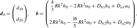 \begin{equation} {\boldsymbol {d}}_0 = \left ( \begin{array}{c} d_{10} \\ \\ d_{20} \end{array} \right)\!, \quad {\boldsymbol {b}} = \left ( \begin{array}{c} \displaystyle \frac {4}{3} R k^2 h_0 - 2 R k^2 \alpha _0 +D_{h1} h_0 + D_{a1} \alpha _0 \\ \\ 2 R k^2 h_0 - \displaystyle \frac {16}{5} R k^2 \alpha _{0} +D_{h2} h_0 + D_{a2} \alpha _0 \end{array} \right)\! , \end{equation}
with the FSI functions of $k$
coming from
$k$
coming from $C_{F_1}$
and
$C_{F_1}$
and $C_{F_2}$
given by
$C_{F_2}$
given by
 \begin{equation} D_{11}(k)= \frac {\pi }{192} \left ( 5745 k^2 - 10848 i k -1056 \right) - \frac {\pi \mathcal{C}(k)}{2} \left (\frac {263}{4} \, i k +59 \right)\! , \end{equation}
 \begin{equation} D_{12}(k)= \frac {\pi }{192} \left ( 41540 k^2 - 80190 i k -8640 \right) - \frac {\pi \mathcal{C}(k)}{2} \left (\frac {3831}{8} \, i k + \frac {1755}{4} \right)\! , \end{equation}
 \begin{equation} D_{21}(k)= \frac {\pi }{128} \left ( 5680 k^2 - 10580 i k -912 \right) - \frac {5 \pi \mathcal{C}(k)}{8} \left (\frac {263}{4} \, i k +59 \right)\! , \end{equation}
 \begin{equation} D_{22}(k)= \frac {\pi }{128} \left ( 41117 k^2 - 78350 i k -7530 \right) - \frac {5\pi \mathcal{C}(k)}{8} \left (\frac {3831}{8} \, i k + \frac {1755}{4} \right)\! , \end{equation}
 \begin{equation} D_{h1}(k)= \frac {5 \pi }{4} k^2 - \pi \mathcal{C}(k) \, i k \,, \quad D_{a1}(k)= \pi \left ( 2 i k - \frac {3}{2} k^2 \right) + \frac {\pi \mathcal{C}(k)}{2} (2 + 3 i k) , \end{equation}
 \begin{equation} D_{h2}(k)= \frac {7 \pi }{4} k^2 - \frac {5 \pi \mathcal{C}(k)}{4} \, i k \,, \quad D_{a1}(k)= \pi \left ( \frac {23}{8}\, i k - \frac {35}{16} k^2 \right) + \frac {5\pi \mathcal{C}(k)}{8} (2 + 3 i k) . \end{equation}
When the FSI is not considered, i.e. when these $D\hbox{-}$
coefficients are not taken into account in (4.1), one obviously recovers the flexural deflection equations in vacuum (2.23). The two first resonant, or natural, frequencies which takes into account the FSI are obtained by minimizing
$D\hbox{-}$
coefficients are not taken into account in (4.1), one obviously recovers the flexural deflection equations in vacuum (2.23). The two first resonant, or natural, frequencies which takes into account the FSI are obtained by minimizing $|\det ({ \mathsf{A}})|$
. They will be denoted by
$|\det ({ \mathsf{A}})|$
. They will be denoted by $k_{r1}$
and
$k_{r1}$
and $k_{r2}$
, and tend to
$k_{r2}$
, and tend to $k_{r10}$
and
$k_{r10}$
and $k_{r20}$
, respectively (given by (2.26) and (2.27)), as the mass ratio
$k_{r20}$
, respectively (given by (2.26) and (2.27)), as the mass ratio $R$
increases for sufficiently large stiffness
$R$
increases for sufficiently large stiffness $S$
(see results below).
$S$
(see results below).
To characterize the magnitude and the phase shift of the flexural deflection for a given heaving and pitching motion one may use the trailing edge displacement, $A_T=|z_s(1,t)|$
, normalized with the rigid foil counterpart
$A_T=|z_s(1,t)|$
, normalized with the rigid foil counterpart $A_{0}$
, and its phase shift
$A_{0}$
, and its phase shift $\psi _t$
from the heaving motion:
$\psi _t$
from the heaving motion:
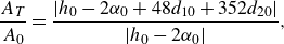 \begin{equation} \frac {A_{T}}{A_{0}}= \frac {|h_0 - 2\alpha _0+ 48 d_{10} +352 d_{20} |}{|h_0 - 2\alpha _0|} , \end{equation}
 \begin{equation} \psi _{t} = {phase} (h_0 - 2\alpha _0+ 48 d_{10} +352 d_{20}) . \end{equation}
Figure 2 shows these two quantities on the $(S,k)\hbox {-}$
plane when
$(S,k)\hbox {-}$
plane when $R=10$
for a pure heaving motion (
$R=10$
for a pure heaving motion ( $\alpha _0 =0$
) set at the leading edge. Also plotted are the first two resonant frequencies, both in vacuum and taking into account the FSI, which in this case are very close to each other for large
$\alpha _0 =0$
) set at the leading edge. Also plotted are the first two resonant frequencies, both in vacuum and taking into account the FSI, which in this case are very close to each other for large $S$
because
$S$
because $R$
is large enough (the inertia of the foil is much greater than that of the fluid). It is observed that the flexural deformation magnitude
$R$
is large enough (the inertia of the foil is much greater than that of the fluid). It is observed that the flexural deformation magnitude $A_T/A_0$
presents local maxima around the two natural frequencies for large stiffness, particularly for
$A_T/A_0$
presents local maxima around the two natural frequencies for large stiffness, particularly for $S$
larger than the stiffness
$S$
larger than the stiffness $S_r$
where the two natural frequencies merge, which in this case with
$S_r$
where the two natural frequencies merge, which in this case with $R=10$
is
$R=10$
is $S_r \approx 1.5$
. The flexural deformation decays very rapidly outside these regions around the two natural frequencies up to the merging point. Also plotted in the figure is the first resonant frequency obtained in Fernandez-Feria & Alaminos-Quesada (Reference Fernandez-Feria and Alaminos-Quesada2021) using a quartic polynomial approximation for
$S_r \approx 1.5$
. The flexural deformation decays very rapidly outside these regions around the two natural frequencies up to the merging point. Also plotted in the figure is the first resonant frequency obtained in Fernandez-Feria & Alaminos-Quesada (Reference Fernandez-Feria and Alaminos-Quesada2021) using a quartic polynomial approximation for $z_s$
, which can only capture the first natural mode. The value of
$z_s$
, which can only capture the first natural mode. The value of $k_{r10}$
in vacuum from this simpler approximation is practically the same as the present one for all
$k_{r10}$
in vacuum from this simpler approximation is practically the same as the present one for all $S$
; when the FSI is considered,
$S$
; when the FSI is considered, $k_{r1}$
from the quartic approximation practically coincides with the present one for
$k_{r1}$
from the quartic approximation practically coincides with the present one for $S$
larger than the merging value
$S$
larger than the merging value $S_r$
(note than in Fernandez-Feria & Alaminos-Quesada (Reference Fernandez-Feria and Alaminos-Quesada2021),
$S_r$
(note than in Fernandez-Feria & Alaminos-Quesada (Reference Fernandez-Feria and Alaminos-Quesada2021), $S$
and
$S$
and $R$
are defined as
$R$
are defined as $S/4$
and
$S/4$
and $R/4$
of the present work, respectively). It is also worth mentioning that the second natural frequency with FSI computed here coincides with that obtained by Floryan & Rowley (Reference Floryan and Rowley2018) from the numerical solution of the full E–B beam equation. In relation to the phase shift of the deformation at the trailing edge, figure 2(b) shows that
$R/4$
of the present work, respectively). It is also worth mentioning that the second natural frequency with FSI computed here coincides with that obtained by Floryan & Rowley (Reference Floryan and Rowley2018) from the numerical solution of the full E–B beam equation. In relation to the phase shift of the deformation at the trailing edge, figure 2(b) shows that $\psi _t \approx -160^o$
when
$\psi _t \approx -160^o$
when $A_T/A_0$
reaches its maximum values around the natural frequencies.
$A_T/A_0$
reaches its maximum values around the natural frequencies.
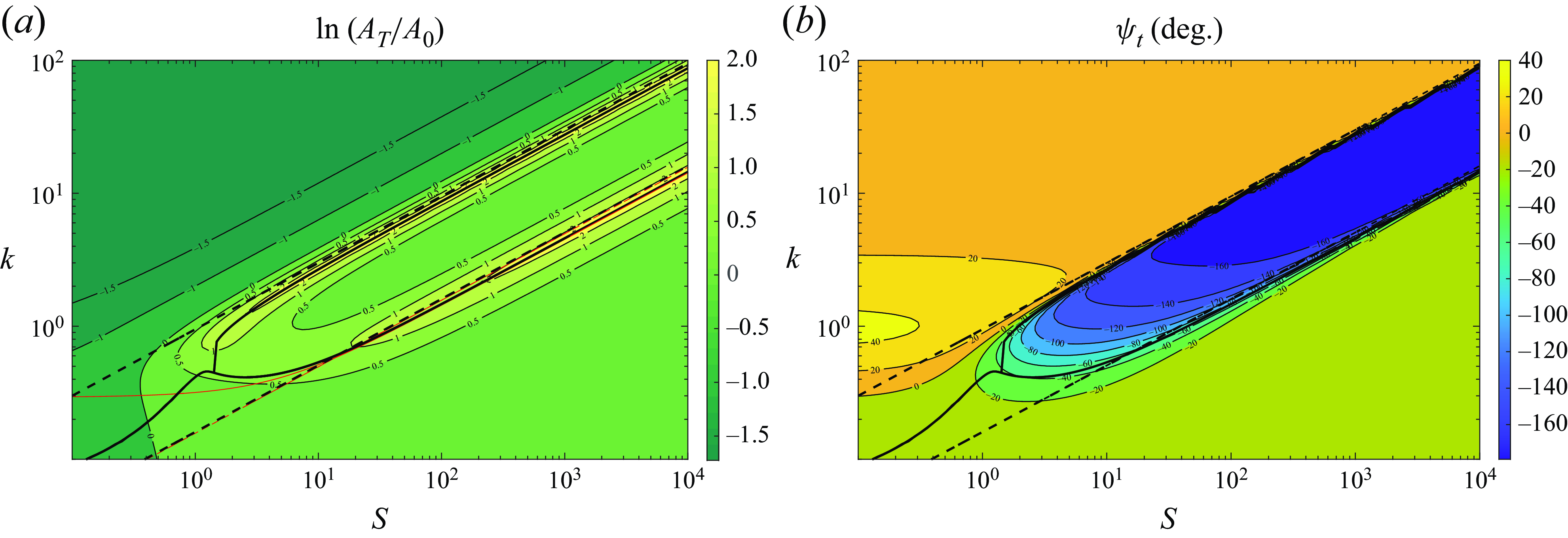
Figure 2. Normalized flexural deflection amplitude at the trailing edge $A_T/A_0$
(a), and its phase shift
$A_T/A_0$
(a), and its phase shift $\psi _t$
(b), for pure heave as
$\psi _t$
(b), for pure heave as $k$
and
$k$
and $S$
are varied when
$S$
are varied when $R=10$
. The thick black lines correspond to
$R=10$
. The thick black lines correspond to $k_{r1}$
and
$k_{r1}$
and $k_{r2}$
, computed by minimizing
$k_{r2}$
, computed by minimizing $|\det ({ \mathsf{A}})|$
, and the corresponding dashed lines are
$|\det ({ \mathsf{A}})|$
, and the corresponding dashed lines are $k_{r10}$
and
$k_{r10}$
and $k_{r20}$
from (2.26) and (2.27). Also shown in (a) with thin red lines are
$k_{r20}$
from (2.26) and (2.27). Also shown in (a) with thin red lines are $k_{r1}$
and
$k_{r1}$
and $k_{r10}$
from Fernandez-Feria & Alaminos-Quesada (Reference Fernandez-Feria and Alaminos-Quesada2021).
$k_{r10}$
from Fernandez-Feria & Alaminos-Quesada (Reference Fernandez-Feria and Alaminos-Quesada2021).
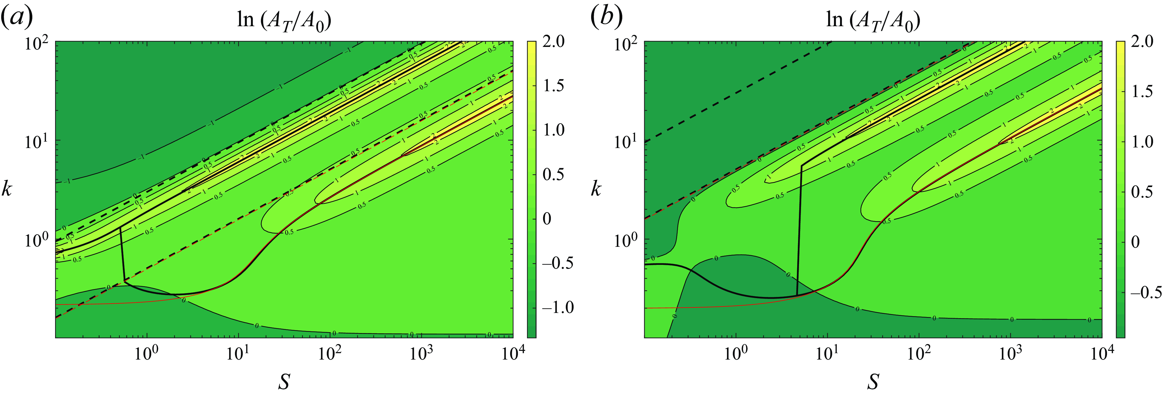
Figure 3. As in figure 2(a), but for $R=1$
(a), and
$R=1$
(a), and $R=0.01$
(b).
$R=0.01$
(b).
As $R$
decreases,
$R$
decreases, $k_{r10}$
and
$k_{r10}$
and $k_{r20}$
grow as
$k_{r20}$
grow as $R^{-1/2}$
(see (2.26) and (2.27)), but
$R^{-1/2}$
(see (2.26) and (2.27)), but $k_{r1}$
and
$k_{r1}$
and $k_{r2}$
grow at a much slower pace, so that the natural frequencies with FSI separate from their vacuum counterparts as the relative inertia of the solid decreases (see figure 3 for
$k_{r2}$
grow at a much slower pace, so that the natural frequencies with FSI separate from their vacuum counterparts as the relative inertia of the solid decreases (see figure 3 for $R=1$
and
$R=1$
and $R=0.01$
). In fact, for
$R=0.01$
). In fact, for $R=0.01$
,
$R=0.01$
, $k_{r2}$
becomes even smaller than
$k_{r2}$
becomes even smaller than $k_{r10}$
. But the qualitative pattern of
$k_{r10}$
. But the qualitative pattern of $A_T/A_0$
remains: local maxima about
$A_T/A_0$
remains: local maxima about $k_{r1}$
and
$k_{r1}$
and $k_{r2}$
for sufficiently large
$k_{r2}$
for sufficiently large $S$
, in any case larger than the stiffness
$S$
, in any case larger than the stiffness $S$
where the two natural frequencies merge, and rapid decay of
$S$
where the two natural frequencies merge, and rapid decay of $A_T/A_0$
outside these regions. It must be recalled that the present approximation fails when the frequency
$A_T/A_0$
outside these regions. It must be recalled that the present approximation fails when the frequency $k$
exceeds
$k$
exceeds $k_{r2}(S,R)$
.
$k_{r2}(S,R)$
.
4.1. Comparison with experimental data. Deflection correction with a nonlinear fluid damping
Although the natural frequencies around which the flexural deflection reaches its maximum are quite well predicted by the present formulation, it is well known that the amplitudes of these resonant deflections are greatly overestimated by the linear theory. Actually, they reach infinity in vacuum (see § 2.2), and, as shown in figures 2 and 3, $A_T/A_0$
may become much larger than unity near the natural frequencies, violating the linear hypothesis. This behaviour can be corrected by taking into account an external resistive term in the E–B equation modelling the lateral (or transverse) fluid dynamic drag (Taylor Reference Taylor1952; Eloy et al. Reference Eloy, Kofman and Schouveiler2012). Since the correction has to be mainly done around the natural frequencies, for outside these regions the flexural deflection amplitude remain within the limits of the linear theory, the use of a nonlinear damping term on the left-hand side of (2.1) of the form
$A_T/A_0$
may become much larger than unity near the natural frequencies, violating the linear hypothesis. This behaviour can be corrected by taking into account an external resistive term in the E–B equation modelling the lateral (or transverse) fluid dynamic drag (Taylor Reference Taylor1952; Eloy et al. Reference Eloy, Kofman and Schouveiler2012). Since the correction has to be mainly done around the natural frequencies, for outside these regions the flexural deflection amplitude remain within the limits of the linear theory, the use of a nonlinear damping term on the left-hand side of (2.1) of the form
 \begin{equation} \frac {1}{2} C_{Dz} \left | \frac {\partial z_s}{\partial t} \right | \frac {\partial z_s}{\partial t} , \end{equation}
where $C_{Dz}$
is an empirically fitted transverse drag coefficient, would be enough (Paraz et al. Reference Paraz, Schouveiler and Eloy2016; Piñeirua et al. Reference Piñeirua, Thiria and Godoy-Diana2017). In fact, only terms involving products of the flexural deflections
$C_{Dz}$
is an empirically fitted transverse drag coefficient, would be enough (Paraz et al. Reference Paraz, Schouveiler and Eloy2016; Piñeirua et al. Reference Piñeirua, Thiria and Godoy-Diana2017). In fact, only terms involving products of the flexural deflections $d_1$
and
$d_1$
and $d_2$
would be relevant in (4.12), because any other quadratic term would be negligible for small pitching and heaving amplitudes. But, for completeness, all the terms are retained.
$d_2$
would be relevant in (4.12), because any other quadratic term would be negligible for small pitching and heaving amplitudes. But, for completeness, all the terms are retained.
In non-dimensional form, the nonlinear damping (4.12) would introduce, for the harmonic motion (2.20)–(2.21), the following terms into the left-hand side of the flexural deflection moment equations (2.12) and (2.13), respectively:
 \begin{align} & i k^2 C_{Dz} \left ( \left | \frac {4}{3} h_0 -2 \alpha _0 +k_{1h1} d_{10} + k_{1h2} d_{20} \right | h_0 + \left | -2 h_0 + \frac {16}{5} \alpha _0 +k_{1a1} d_{10} + k_{1a2} d_{20} \right | \alpha _0 \right .\nonumber \\ &\qquad \qquad + \left | k_{1h1} h_0+ k_{1a1} \alpha _0 + k_{111} d_{10}+k_{112} d_{20} \right | d_{10} \nonumber \\ &\qquad\! \qquad \left. + \,\left | k_{1h2} h_0+ k_{1a2} \alpha _0 +k_{112} d_{10}+k_{122} d_{20} \right | d_{20} \vphantom{\frac{1}{1}}\right)\!, \end{align}
and
 \begin{align} & i k^2 C_{Dz} \left ( \left | 2 h_0 - \frac {16}{5} \alpha _0 +k_{2h1} d_{10} + k_{2h2} d_{20} \right | h_0 \right. \nonumber\\ &\qquad \qquad+ \left | - \frac {16}{5} h_0 + \frac {16}{3} \alpha _0 +k_{2a1} d_{10} + k_{2a2} d_{20} \right | \alpha _0 \nonumber\\ & \qquad \qquad + \left | k_{2h1} h_0+ k_{2a1} \alpha _0 + k_{211} d_{10}+k_{212} d_{20} \right | d_{10} \nonumber\\ & \qquad \qquad \left. + \,\left | k_{2h2} h_0+ k_{2a2} \alpha _0 + k_{212} d_{10}+k_{222} d_{20} \right | d_{20} \vphantom{\frac{1}{1}}\right)\!, \end{align}
where the $k_{\ldots }\hbox{-}$
constants are given in Appendix B. Thus, instead of (4.1), the equation for determining the flexural deflection amplitude and phase becomes
$k_{\ldots }\hbox{-}$
constants are given in Appendix B. Thus, instead of (4.1), the equation for determining the flexural deflection amplitude and phase becomes
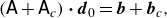 \begin{equation} \left ( { \mathsf{A}} + { \mathsf{A}}_c \right) \boldsymbol{\cdot} {\boldsymbol {d}}_0 = {\boldsymbol {b}} + {\boldsymbol {b}}_c , \end{equation}
where the new matrix ${ \mathsf{A}}_c$
and vector
${ \mathsf{A}}_c$
and vector ${\boldsymbol {b}}_c$
, which depend on
${\boldsymbol {b}}_c$
, which depend on ${\boldsymbol {d}}_0$
, are also given in Appendix B.
${\boldsymbol {d}}_0$
, are also given in Appendix B.
This is a nonlinear equation for ${\boldsymbol {d}}_0$
which can easily be solved iteratively starting from the solution for
${\boldsymbol {d}}_0$
which can easily be solved iteratively starting from the solution for $C_{Dz}=0$
given by (4.1). Since both
$C_{Dz}=0$
given by (4.1). Since both ${ \mathsf{A}}_c$
and
${ \mathsf{A}}_c$
and ${\boldsymbol {b}}_c$
are proportional to
${\boldsymbol {b}}_c$
are proportional to $k^2$
, the correction to the linear solution will be more important as the frequency
$k^2$
, the correction to the linear solution will be more important as the frequency $k$
increases, which is consistent with the fact that the largest deflection amplitude coming from the linear theory is commonly observed at the second natural frequency
$k$
increases, which is consistent with the fact that the largest deflection amplitude coming from the linear theory is commonly observed at the second natural frequency $k_{r2}$
, so that, as we shall see below, the nonlinear damping correction must be the greatest around this frequency.
$k_{r2}$
, so that, as we shall see below, the nonlinear damping correction must be the greatest around this frequency.
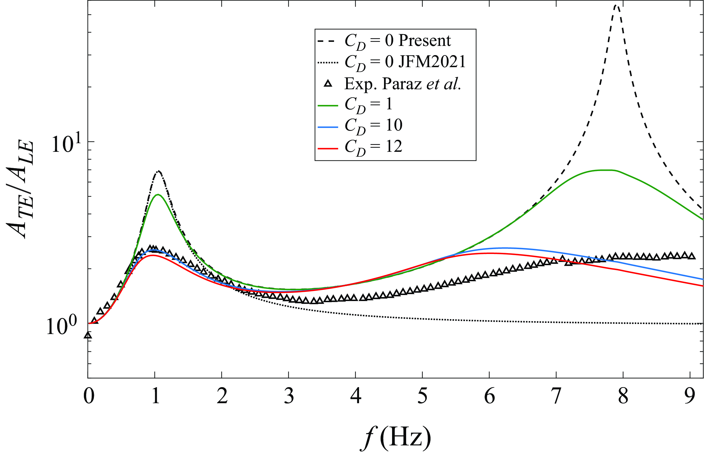
Figure 4. Comparison of experimental results by Paraz, Eloy & Schouveiler (Reference Paraz, Eloy and Schouveiler2014) for $A_T/A_0=A_{TE}/A_{LE}$
versus the frequency (triangles, case
$A_T/A_0=A_{TE}/A_{LE}$
versus the frequency (triangles, case $B=0.053$
N m in their figure 5a) with the present linear results (
$B=0.053$
N m in their figure 5a) with the present linear results ( $C_{Dz}=0$
, dashed line), and damped with
$C_{Dz}=0$
, dashed line), and damped with $C_{Dz}=1, \,10$
and
$C_{Dz}=1, \,10$
and $12$
(solid lines). Also shown with a dotted line is the linear result from Fernandez-Feria & Alaminos-Quesada (Reference Fernandez-Feria and Alaminos-Quesada2021), which only captures the first natural frequency.
$12$
(solid lines). Also shown with a dotted line is the linear result from Fernandez-Feria & Alaminos-Quesada (Reference Fernandez-Feria and Alaminos-Quesada2021), which only captures the first natural frequency.
Figure 4 shows a comparison of the flexural deflection amplitude obtained from the present theoretical formulation with experimental results reported by Paraz et al. (Reference Paraz, Eloy and Schouveiler2014) for a flexible plate with $c=12$
cm undergoing a pure heaving motion in a water current with velocity
$c=12$
cm undergoing a pure heaving motion in a water current with velocity $U=0.05$
m s–1 (
$U=0.05$
m s–1 ( $Re=U c/\nu = 6000$
). The mass ratio of the foil is
$Re=U c/\nu = 6000$
). The mass ratio of the foil is $R=0.16$
and its bending rigidity
$R=0.16$
and its bending rigidity $0.053$
N m, corresponding to the non-dimensional stiffness
$0.053$
N m, corresponding to the non-dimensional stiffness $S=589$
in the present notation. This example also serves to illustrate how the nonlinear fluid damping described above corrects the flexural deflection amplitude as the drag coefficient
$S=589$
in the present notation. This example also serves to illustrate how the nonlinear fluid damping described above corrects the flexural deflection amplitude as the drag coefficient $C_{Dz}$
and the forcing frequency
$C_{Dz}$
and the forcing frequency $f$
are varied. The figure plots the trailing-edge amplitude
$f$
are varied. The figure plots the trailing-edge amplitude $A_{TE}$
normalized with the heaving amplitude,
$A_{TE}$
normalized with the heaving amplitude, $A_{LE}=0.004$
m (
$A_{LE}=0.004$
m ( $h_0 \simeq 0.067$
), a ratio that coincides with
$h_0 \simeq 0.067$
), a ratio that coincides with $A_T/A_0$
defined in (4.10) for a pure heaving motion, versus the dimensional frequency in hertz. The present linear theory with no damping (
$A_T/A_0$
defined in (4.10) for a pure heaving motion, versus the dimensional frequency in hertz. The present linear theory with no damping ( $C_{Dz}=0$
, dashed line) presents two marked maxima at the first two natural frequencies,
$C_{Dz}=0$
, dashed line) presents two marked maxima at the first two natural frequencies, $f_{r1}=1.03$
Hz and
$f_{r1}=1.03$
Hz and $f_{r2}=7.90$
Hz. Also shown for comparison sake is the deflection obtained with a quartic polynomial approximation for
$f_{r2}=7.90$
Hz. Also shown for comparison sake is the deflection obtained with a quartic polynomial approximation for $z_s$
in Fernandez-Feria & Alaminos-Quesada (Reference Fernandez-Feria and Alaminos-Quesada2021) (dotted line with
$z_s$
in Fernandez-Feria & Alaminos-Quesada (Reference Fernandez-Feria and Alaminos-Quesada2021) (dotted line with $C_{Dz}=0$
), which captures only the first resonant frequency, obviously coinciding with the present results around
$C_{Dz}=0$
), which captures only the first resonant frequency, obviously coinciding with the present results around $f_{r1}$
, but decaying beyond that frequency without presenting any other peak. The trailing edge deflection ratio
$f_{r1}$
, but decaying beyond that frequency without presenting any other peak. The trailing edge deflection ratio $A_T/A_0$
is also plotted for three values of
$A_T/A_0$
is also plotted for three values of $C_{Dz} \ne 0$
to show how the linear resonant peaks are damped as
$C_{Dz} \ne 0$
to show how the linear resonant peaks are damped as $C_{Dz}$
increases, but barely affecting the rest of the deflection amplitude. It is found that the present theoretical results with
$C_{Dz}$
increases, but barely affecting the rest of the deflection amplitude. It is found that the present theoretical results with $C_{Dz}=10$
best fit the experimental results around the first natural frequency, which is close to the value
$C_{Dz}=10$
best fit the experimental results around the first natural frequency, which is close to the value $C_{Dz}=12$
found by Paraz et al. (Reference Paraz, Schouveiler and Eloy2016) to best fit their analytical model with the experimental data. The present results with
$C_{Dz}=12$
found by Paraz et al. (Reference Paraz, Schouveiler and Eloy2016) to best fit their analytical model with the experimental data. The present results with $C_{Dz}=12$
are also plotted to show that their differences with
$C_{Dz}=12$
are also plotted to show that their differences with $C_{Dz}=10$
are quite small. Around the second natural frequency, the agreement of the present results (using either
$C_{Dz}=10$
are quite small. Around the second natural frequency, the agreement of the present results (using either $C_{Dz}=10$
or
$C_{Dz}=10$
or $12$
) with the experimental data is poorer than around the first natural frequency, but they qualitatively capture the magnitude of the experimental deflection. Figure 5 illustrates the shape of the flexible plate along a flapping cycle at the two natural frequencies.
$12$
) with the experimental data is poorer than around the first natural frequency, but they qualitatively capture the magnitude of the experimental deflection. Figure 5 illustrates the shape of the flexible plate along a flapping cycle at the two natural frequencies.
Figure 5. Plate shape at different times for the same case plotted in figure 4 ( $h_0=0.067$
,
$h_0=0.067$
, $\alpha _0=0$
,
$\alpha _0=0$
, $R=0.16$
,
$R=0.16$
, $S=589$
) at the first (a) and second (b) resonant frequencies.
$S=589$
) at the first (a) and second (b) resonant frequencies.
Further comparison of the present flexural deflection theoretical results with other experimental data is provided in § 5.4.
5. Propulsion performance
5.1. Thrust coefficient
Before deriving the expression for the thrust force generated by the flexible foil’s kinematics, (2.8)–(2.9), in the present framework of linear potential theory, it is instructive to write the lift coefficient (2.15) in terms of the vorticity distribution, but not in the form (3.9) used in § 3.1, but according to the general vortical impulse theory (Wu Reference Wu1981; Saffman Reference Saffman1992).
Starting from (3.9) and using Kelvin’s theorem, $\int _{-1}^1 \varpi _s(x,t) {\textrm d}x + \int _1^\infty \varpi _e (x,t) {\textrm d}x =0$
, it can be written as
$\int _{-1}^1 \varpi _s(x,t) {\textrm d}x + \int _1^\infty \varpi _e (x,t) {\textrm d}x =0$
, it can be written as
 \begin{equation} C_L(t)= - \frac {\textrm d}{{\textrm d}t} \int _{-1}^1 x \varpi _s(x,t) {\textrm d}x - \frac {\textrm d}{{\textrm d}t} \int _1^\infty \varpi _e(x,t) {\textrm d}x - \int _1^\infty \varpi _e(x,t) {\textrm d} x . \end{equation}
Now, since $\varpi _e(x,t)=\varpi _e(X)$
, with
$\varpi _e(x,t)=\varpi _e(X)$
, with $X=x-t$
(von Kármán & Sears Reference von Kármán and Sears1938),
$X=x-t$
(von Kármán & Sears Reference von Kármán and Sears1938),
 \begin{align} \frac {\textrm d}{{\textrm d}t} \int _1^\infty (x-1) \varpi _e(X) {\textrm d}x = \frac {\textrm d}{{\textrm d}t} \int _{1-t}^\infty (X+t-1) \varpi _e(X) {\textrm d} X = \int _1^\infty \varpi _e(x,t) {\textrm d}x . \end{align}
Substituting this expression into the last term of (5.1) one gets the lift coefficient as the $z\hbox{-}$
component of the 2-D force
$z\hbox{-}$
component of the 2-D force $\boldsymbol {F}$
in terms of vortical impulse,
$\boldsymbol {F}$
in terms of vortical impulse, ${\boldsymbol {F}} = - \rho d (\int _{\mathcal{V}_\infty } ({\boldsymbol {x}} \wedge {\boldsymbol{\omega }}) {\textrm d}\mathcal{V})/{\textrm d} t$
, where
${\boldsymbol {F}} = - \rho d (\int _{\mathcal{V}_\infty } ({\boldsymbol {x}} \wedge {\boldsymbol{\omega }}) {\textrm d}\mathcal{V})/{\textrm d} t$
, where $\boldsymbol{\omega }$
is the vorticity field and
$\boldsymbol{\omega }$
is the vorticity field and $\mathcal{V}_\infty$
the entire fluid domain. In non-dimensional form and in the small-amplitude linearized limit,
$\mathcal{V}_\infty$
the entire fluid domain. In non-dimensional form and in the small-amplitude linearized limit,
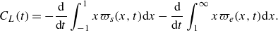 \begin{equation} C_L(t)= - \frac {\textrm d}{{\textrm d}t} \int _{-1}^1 x \varpi _s(x,t) {\textrm d}x - \frac {\textrm d}{{\textrm d}t} \int _1^\infty x \varpi _e(x,t) {\textrm d}x . \end{equation}
This expression was already used by von Kármán & Sears (Reference von Kármán and Sears1938) in their pioneering work on unsteady airfoil theory, recovering the previous result by Theodorsen (Reference Theodorsen1935) from the standard expression (2.15) for a rigid foil undergoing a general harmonic pitching and heaving motion of small amplitude. Likewise, the non-dimensional $x\hbox{-}$
component of the force
$x\hbox{-}$
component of the force $C_x$
, or better, the thrust coefficient
$C_x$
, or better, the thrust coefficient $C_T=-C_x$
, can be written as
$C_T=-C_x$
, can be written as
 \begin{equation} C_T(t)= - \frac {\textrm d}{{\textrm d}t} \int _{-1}^1 z_s(x,t) \varpi _s(x,t) {\textrm d}x - \frac {\textrm d}{{\textrm d}t} \int _1^\infty z_e(x,t) \varpi _e(x,t) {\textrm d}x , \end{equation}
where $z_e(x,t)$
is the displacement of the vortex wake in the
$z_e(x,t)$
is the displacement of the vortex wake in the $z\hbox{-}$
direction. This expression, valid for
$z\hbox{-}$
direction. This expression, valid for $|z_s| \ll 1$
and
$|z_s| \ll 1$
and $|z_e| \ll 1$
as it is (5.3), is now used for the flexible foil’s kinematics (2.8)–(2.9).
$|z_e| \ll 1$
as it is (5.3), is now used for the flexible foil’s kinematics (2.8)–(2.9).
Assuming that $z_e(x,t)$
is, like
$z_e(x,t)$
is, like $\varpi _e(x,t)$
, a function only of
$\varpi _e(x,t)$
, a function only of $X=x-t$
, i.e. that the wake is stationary relative to the fluid (von Kármán & Sears Reference von Kármán and Sears1938), the last term can be written as
$X=x-t$
, i.e. that the wake is stationary relative to the fluid (von Kármán & Sears Reference von Kármán and Sears1938), the last term can be written as
 \begin{equation} - \frac {\textrm d}{{\textrm d}t} \int _1^\infty z_e(x,t) \varpi _e(x,t) {\textrm d}x = - z_e(1,t) \varpi _e(1,t) = - z_s(1,t) \varpi _e(1,t) . \end{equation}
The thrust force obtained with this assumption in the simplest case of a rigid pitching and heaving foil has shown to compare very well with several sets of experimental data for small-amplitude oscillations (Fernandez-Feria Reference Fernandez-Feria2016, Reference Fernandez-Feria2017; Alaminos-Quesada Reference Alaminos-Quesada2021).
Taking into account (3.3), the first term in (5.4) contains terms associated with $\varpi _0(x,t)$
and to
$\varpi _0(x,t)$
and to $\varpi _{se}(x,t)$
. The terms corresponding to
$\varpi _{se}(x,t)$
. The terms corresponding to $\varpi _0$
are easily computed using (2.8) and (3.11), to yield
$\varpi _0$
are easily computed using (2.8) and (3.11), to yield
 \begin{equation}\! - \frac {\textrm d}{{\textrm d}t}\! \int _{-1}^1 \! z_s(x,t) \varpi _0(x,t) {\textrm d}x = - \frac {\textrm d}{{\textrm d}t} \left [ h(t) \Gamma _0(t) + \alpha (t) \Gamma _a(t) + d_1(t) \Gamma _{d_1}(t) + d_2(t) \Gamma _{d_2}(t) \right]\!, \end{equation}
where $\Gamma _0(t)$
, defined in (3.7), is given by (3.15), whereas the other functions
$\Gamma _0(t)$
, defined in (3.7), is given by (3.15), whereas the other functions $\Gamma _{\ldots } (t)$
are given in Appendix C. It is understood that the terms inside brackets are the product of the real parts of each factor; e.g.
$\Gamma _{\ldots } (t)$
are given in Appendix C. It is understood that the terms inside brackets are the product of the real parts of each factor; e.g. $\textrm{Re} [h(t)] \textrm{Re} [\Gamma _0(t)]$
.
$\textrm{Re} [h(t)] \textrm{Re} [\Gamma _0(t)]$
.
For the terms coming from $\varpi _{se}$
, one can first use Kelvin’s theorem (3.8), and then make use the expression (3.5) for
$\varpi _{se}$
, one can first use Kelvin’s theorem (3.8), and then make use the expression (3.5) for $\varpi _{se}$
to integrate in
$\varpi _{se}$
to integrate in $x$
(except for the term corresponding to
$x$
(except for the term corresponding to $h(t)$
in
$h(t)$
in $z_s(x,t)$
for which this last step is not needed):
$z_s(x,t)$
for which this last step is not needed):
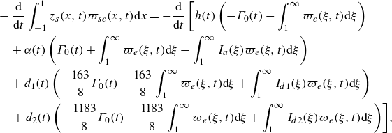 \begin{align} &- \frac {\textrm d}{{\textrm d}t} \int _{-1}^1 z_s(x,t) \varpi _{se}(x,t) {\textrm d}x = - \frac {\textrm d}{{\textrm d}t} \left [ h(t) \left ( - \Gamma _0(t) - \int _1^\infty \varpi _e(\xi,t) {\textrm d}\xi \right) \right. \nonumber \\ &\quad + \alpha (t) \left (\Gamma _0(t) + \int _1^\infty \varpi _e(\xi,t) {\textrm d}\xi - \int _1^\infty I_a(\xi) \varpi _e(\xi,t) {\textrm d}\xi \right) \nonumber \\ &\quad + d_1(t) \left ( - \frac {163}{8} \Gamma _0(t) - \frac {163}{8} \int _1^\infty \varpi _e(\xi,t) {\textrm d}\xi + \int _1^\infty I_{d1}(\xi) \varpi _e(\xi,t) {\textrm d}\xi \right) \nonumber \\ &\quad \left. +\, d_2(t) \left ( - \frac {1183}{8} \Gamma _0(t) - \frac {1183}{8} \int _1^\infty \varpi _e(\xi,t) {\textrm d}\xi + \int _1^\infty I_{d2}(\xi) \varpi _e(\xi,t) {\textrm d}\xi \right) \right]\!, \end{align}
where
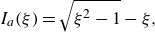 \begin{equation} I_a(\xi) = \sqrt {\xi ^2-1}-\xi , \end{equation}
 \begin{equation} I_{d1}(\xi) = \frac {1}{8} \left [27-224 \xi -48 \xi ^2+32 \xi ^3-8 \xi ^4+ \sqrt {\xi ^2-1} \left (8 \xi ^3-32 \xi ^2+52 \xi +208\right)\right]\!, \end{equation}
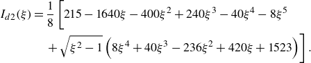 \begin{align} I_{d2}(\xi) & = \frac {1}{8} \left [215-1640 \xi -400 \xi ^2+240 \xi ^3-40 \xi ^4-8 \xi ^5 \vphantom{\frac{1}{1}}\right.\nonumber \\ &\quad \left. +\, \sqrt {\xi ^2-1} \left (8 \xi ^4 + 40\xi ^3-236 \xi ^2+420 \xi +1523\right)\right] . \end{align}
The factors $163/8$
and
$163/8$
and $1183/8$
appear when applying Kelvin’s theorem to the terms corresponding to
$1183/8$
appear when applying Kelvin’s theorem to the terms corresponding to $d_1$
and
$d_1$
and $d_2$
, respectively, because these factors are subtracted to the functions of
$d_2$
, respectively, because these factors are subtracted to the functions of $x$
multiplying
$x$
multiplying $d_1$
and
$d_1$
and $d_2$
in
$d_2$
in $z_s$
, so that the functions
$z_s$
, so that the functions $I_{d1}(\xi)$
and
$I_{d1}(\xi)$
and $I_{d2}(\xi)$
appearing in the integrals in
$I_{d2}(\xi)$
appearing in the integrals in $\xi$
are regular at the leading edge
$\xi$
are regular at the leading edge $\xi =1$
; particularly, their values at
$\xi =1$
; particularly, their values at $\xi =1$
are
$\xi =1$
are
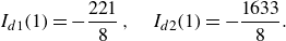 \begin{equation} I_{d1}(1) = - \frac {221}{8} \,, \quad I_{d2}(1) = - \frac {1633}{8} . \end{equation}
This regularity is important to compute the time derivatives of these integrals taking into account that $\varpi _e(\xi,t) = \varpi _e(X)$
, with
$\varpi _e(\xi,t) = \varpi _e(X)$
, with $X=\xi -t$
, so that, for any function
$X=\xi -t$
, so that, for any function $G(\xi)$
regular at
$G(\xi)$
regular at $\xi =1$
, the time derivative can be written as (von Kármán & Sears Reference von Kármán and Sears1938)
$\xi =1$
, the time derivative can be written as (von Kármán & Sears Reference von Kármán and Sears1938)
 \begin{align} \frac {\textrm d}{{\textrm d}t} \int _1^\infty G(\xi) \varpi _e(\xi,t) {\textrm d}x = \int _1^\infty \frac {{\textrm d}G(\xi)}{{\textrm d}\xi } \varpi _e(\xi,t) {\textrm d}\xi + G(1) \varpi _e(1,t) . \end{align}
Performing these time derivatives in (5.7) and then the resulting integrals in $\xi$
, taking into account that
$\xi$
, taking into account that $\varpi _e(\xi,t)$
can be written as (see text above (3.13))
$\varpi _e(\xi,t)$
can be written as (see text above (3.13))
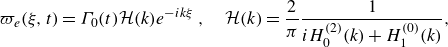 \begin{equation} \varpi _e(\xi,t)= \Gamma _0(t) \mathcal{H}(k) e^{-i k \xi } \,, \quad \mathcal{H} (k) = \frac {2}{\pi } \frac {1}{i H_0^{(2)} (k) + H_1^{(0)}(k) } , \end{equation}
and substituting (5.5), (5.6) and (5.7) into (5.4), the thrust coefficient can finally be expressed as
 \begin{equation} C_T(t)= C_{T0}(t) + C_{Tc}(t) , \end{equation}
with
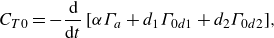 \begin{equation} C_{T0}= - \frac {\textrm d}{{\textrm d}t} \left [ \alpha \Gamma _a +d_1 \Gamma _{0d1} + d_2 \Gamma _{0d2} \right]\!, \end{equation}
and
 \begin{align} C_{Tc} &= \left ( \dot {h}- \dot {\alpha } + \frac {163}{8} \dot {d}_1+ \frac {1183}{8} \dot {d}_2 \right) [\Gamma _0 \mathcal{C}_h] + \dot {\alpha } [\Gamma _0 \mathcal{C}_{a1}] + \alpha [\Gamma _0 \mathcal{C}_{a0}] \nonumber \\ &\quad + \dot {d}_1 [\Gamma _0 \mathcal{C}_{d11}] + d_1 [\Gamma _0 \mathcal{C}_{d10}] + \dot {d}_2 [\Gamma _0 \mathcal{C}_{d21}] + d_2 [\Gamma _0 \mathcal{C}_{d20}] , \end{align}
where the different functions $\Gamma _{0 \ldots }(t)$
and complex functions
$\Gamma _{0 \ldots }(t)$
and complex functions $\mathcal{C}_{\ldots }(k)$
are given in the Appendices C and D, respectively. Note that all the terms involving
$\mathcal{C}_{\ldots }(k)$
are given in the Appendices C and D, respectively. Note that all the terms involving $\varpi _e(1,t)$
in (5.7), some of them affected by the constants (5.11) after time derivation, cancel exactly out, this being an indication of the coherence of the method and the correctness of the computations. All the terms in (5.15) and (5.16) are actually the product of the real parts of two factors, the second one always written between brackets in (5.16) for clarity sake. The new contributions to
$\varpi _e(1,t)$
in (5.7), some of them affected by the constants (5.11) after time derivation, cancel exactly out, this being an indication of the coherence of the method and the correctness of the computations. All the terms in (5.15) and (5.16) are actually the product of the real parts of two factors, the second one always written between brackets in (5.16) for clarity sake. The new contributions to $C_T$
due to the second flexural mode
$C_T$
due to the second flexural mode $d_2(t)$
are, in addition to those which are explicit in (5.15)–(5.16), scattered inside the different functions
$d_2(t)$
are, in addition to those which are explicit in (5.15)–(5.16), scattered inside the different functions $\Gamma _{0\ldots }(t)$
(see Appendix C). With the use of these
$\Gamma _{0\ldots }(t)$
(see Appendix C). With the use of these $\Gamma _{0\ldots }$
functions, the present notation (5.14)–(5.16) is more compact, and with a clearer separation between added-mas and circulatory terms, than in Fernandez-Feria & Alaminos-Quesada (Reference Fernandez-Feria and Alaminos-Quesada2021).
$\Gamma _{0\ldots }$
functions, the present notation (5.14)–(5.16) is more compact, and with a clearer separation between added-mas and circulatory terms, than in Fernandez-Feria & Alaminos-Quesada (Reference Fernandez-Feria and Alaminos-Quesada2021).
5.2. Cycle-averaged thrust
Time-averaged quantities over the flapping cycle $2 \pi /k$
are more useful for practical applications than the instantaneous ones. Thus, one may define the cycle-averaged (non-dimensional) thrust as
$2 \pi /k$
are more useful for practical applications than the instantaneous ones. Thus, one may define the cycle-averaged (non-dimensional) thrust as
 \begin{equation} \overline {C}_T= \frac {k}{2 \pi } \int _t^{t+ 2 \pi /k} C_T(t) {\textrm d} t . \end{equation}
Clearly, the time average of the added-mass component (5.15) vanishes exactly because it is the time derivative of products of periodic functions of $t$
with zero mean. Therefore, all the time-averaged thrust comes from the circulatory part (5.16), and can be written as
$t$
with zero mean. Therefore, all the time-averaged thrust comes from the circulatory part (5.16), and can be written as
 \begin{align} \overline {C}_T = \overline {C}_{Tc} &= t_h h_0^2+t_a a_0^2 + t_{d_1} d_{1m}^2 + t_{d_2} d_{2m}^2 + t_{ha} h_0 a_0 +t_{hd1} h_0 d_{1m} \nonumber \\ &\quad +t_{hd2} h_0 d_{2m} + t_{ad1} a_0 d_{1m} +t_{ad2} a_0 d_{2m} + t_{d1d2} d_{1m} d_{2m} , \end{align}
where the coefficients $t_h, t_a, t_{d_1}, t_{d_2}, t_{ha}, t_{hd1}, t_{hd2}, t_{ad1}, t_{ad2}$
and
$t_h, t_a, t_{d_1}, t_{d_2}, t_{ha}, t_{hd1}, t_{hd2}, t_{ad1}, t_{ad2}$
and $t_{d1d2}$
multiplying the heave, pitch and flexural deformation amplitudes, which are functions of the reduced frequency
$t_{d1d2}$
multiplying the heave, pitch and flexural deformation amplitudes, which are functions of the reduced frequency $k$
, and eventually of the phases
$k$
, and eventually of the phases $\phi$
,
$\phi$
, $\psi _1$
and
$\psi _1$
and $\psi _2$
, are given in Appendix E. For
$\psi _2$
, are given in Appendix E. For $d_{2m}=0$
this expression coincides with that in Fernandez-Feria & Alaminos-Quesada (Reference Fernandez-Feria and Alaminos-Quesada2021) for a pivot axis at the leading edge, though written in a slightly different notation.
$d_{2m}=0$
this expression coincides with that in Fernandez-Feria & Alaminos-Quesada (Reference Fernandez-Feria and Alaminos-Quesada2021) for a pivot axis at the leading edge, though written in a slightly different notation.
An offset drag $C_{Dx}$
is usually subtracted to this theoretical expression coming from the linear potential theory to account for the streamwise viscous friction. Its value is obviously much smaller than the transversal drag coefficient
$C_{Dx}$
is usually subtracted to this theoretical expression coming from the linear potential theory to account for the streamwise viscous friction. Its value is obviously much smaller than the transversal drag coefficient $C_{Dz}$
used above to account for the nonlinear viscous damping of the flexural deflection amplitude near the resonant frequencies. Typically,
$C_{Dz}$
used above to account for the nonlinear viscous damping of the flexural deflection amplitude near the resonant frequencies. Typically, $C_{Dx} \approx 0.05$
for small amplitude pitching and heaving motions (Mackowski & Williamson Reference Mackowski and Williamson2015; Senturk & Smits Reference Senturk and Smits2019). Its correction to
$C_{Dx} \approx 0.05$
for small amplitude pitching and heaving motions (Mackowski & Williamson Reference Mackowski and Williamson2015; Senturk & Smits Reference Senturk and Smits2019). Its correction to $\overline {C}_T$
is usually quite irrelevant, except for very small frequencies, since the theoretical
$\overline {C}_T$
is usually quite irrelevant, except for very small frequencies, since the theoretical $\overline {C}_T \to 0$
as
$\overline {C}_T \to 0$
as $k \to 0$
. However small, its use important to avoid an unphysical singularity in the efficiency as
$k \to 0$
. However small, its use important to avoid an unphysical singularity in the efficiency as $k \to 0$
(e.g. Mackowski & Williamson Reference Mackowski and Williamson2015; Fernandez-Feria Reference Fernandez-Feria2017).
$k \to 0$
(e.g. Mackowski & Williamson Reference Mackowski and Williamson2015; Fernandez-Feria Reference Fernandez-Feria2017).
5.3. Power coefficient and efficiency
The power required to generate the pitching and heaving motion about the leading edge is given, in non-dimensional form, by
 \begin{equation} C_P(t)= \dot {h}(t) C_{L_p}(t) - 2 \dot {\alpha }(t) C_{M_p}(t) . \end{equation}
On using (2.10)–(2.11) and the results of §§ 3.1 and 3.2, it can be written as
 \begin{equation} C_P= C_{P_R} + C_{P_F} = C_{P_R}+ C_{P_0}+C_{P_c} , \end{equation}
where
 \begin{equation} C_{P_R} = R \left [ \dot {h} \left ( \ddot {h} - \ddot {\alpha } + \frac {96}{5} \ddot {d}_1 + \frac {416}{3} \ddot {d}_2 \right) - 2 \dot {\alpha } \left ( \frac {1}{2} \ddot {h} - \frac {2}{3} \ddot {\alpha } + \frac {208}{15} \ddot {d}_1 + \frac {704}{7} \ddot {d}_2 \right) \right] \end{equation}
is the contribution due to the inertia of the foil of mass ratio $R$
, whereas
$R$
, whereas
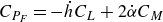 \begin{equation} C_{P_F} = - \dot {h} C_L + 2 \dot {\alpha } C_M \end{equation}
is the fluid contribution, which in turn can be decomposed into an added-mass part, associated with the fluid inertia, and circulatory part,
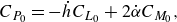 \begin{equation} C_{P_0} = - \dot {h} C_{L_0} + 2 \dot {\alpha } C_{M_0} , \end{equation}
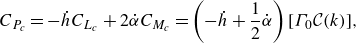 \begin{equation} C_{P_c} = - \dot {h} C_{L_c} + 2 \dot {\alpha } C_{M_c} = \left ( - \dot {h} + \frac {1}{2} \dot {\alpha } \right) [\Gamma _0 \mathcal{C}(k)] , \end{equation}
where $C_{L_0}$
and
$C_{L_0}$
and $C_{M_0}$
are given by (3.12) and (3.19), respectively, and use has been made of (3.13) and (3.20) for
$C_{M_0}$
are given by (3.12) and (3.19), respectively, and use has been made of (3.13) and (3.20) for $C_{L_c}$
and
$C_{L_c}$
and $C_{M_c}$
. The contribution to
$C_{M_c}$
. The contribution to $C_P$
associated with the nonlinear damping term (4.12) in (2.10)–(2.11) has been neglected because it has already used to damp the resonant peaks in the flexural deformation amplitude through its inclusion in (2.12) and (2.13), so that the resulting cubic terms from this nonlinear damping in
$C_P$
associated with the nonlinear damping term (4.12) in (2.10)–(2.11) has been neglected because it has already used to damp the resonant peaks in the flexural deformation amplitude through its inclusion in (2.12) and (2.13), so that the resulting cubic terms from this nonlinear damping in $\dot {h}C_{L_p}$
and
$\dot {h}C_{L_p}$
and $\dot {\alpha } C_{M_p}$
become negligible once
$\dot {\alpha } C_{M_p}$
become negligible once $|d_1|$
and
$|d_1|$
and $|d_2|$
are small.
$|d_2|$
are small.
The time-averaged power coefficient,
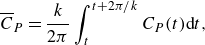 \begin{equation} \overline {C}_P = \frac {k}{2 \pi } \int _t^{t+ 2 \pi /k} C_P(t) {\textrm d} t , \end{equation}
can also be decomposed into the above three contributions. The contribution from the inertia of the foil vanishes for a rigid foil (Fernandez-Feria Reference Fernandez-Feria2023), i.e. when the flexural deflection amplitudes $d_{1m}$
and
$d_{1m}$
and $d_{2m}$
are zero:
$d_{2m}$
are zero:
 \begin{align} \overline {C}_{P_R} &= - \frac {16}{105} R k^3 \left \{ d_{1m} \left [ 91 a_0 \sin (\phi -\psi _1) + 63 h_0 \sin \psi _1 \right] \right. \nonumber \\ &\quad\left. +\, d_{2m} \left [ 660 a_0 \sin (\phi -\psi _2) + 455 h_0 \sin \psi _2 \right] \right \} . \end{align}
This contribution is important at high frequencies when $R$
is not small, e.g. for a flapping foil in air. As it will seen in the results reported below, it may help to reduce the power consumption and thus to increase the propulsion efficiency for large
$R$
is not small, e.g. for a flapping foil in air. As it will seen in the results reported below, it may help to reduce the power consumption and thus to increase the propulsion efficiency for large $R$
.
$R$
.
In general, the total time-averaged power coefficient can be written as
 \begin{align} \overline {C}_{P}= p_h h_0^2+p_a a_0^2 + p_{ha} h_0 a_0 +p_{hd1} h_0 d_{1m} +p_{hd2} h_0 d_{2m} + p_{ad1} a_0 d_{1m} +p_{ad2} a_0 d_{2m} , \\[-15pt] \nonumber\end{align}
where the coefficients $p_h, p_a, p_{ha}, p_{hd1}, p_{hd2}, p_{ad1}$
and
$p_h, p_a, p_{ha}, p_{hd1}, p_{hd2}, p_{ad1}$
and $p_{ad2}$
, which are functions of the reduced frequency
$p_{ad2}$
, which are functions of the reduced frequency $k$
, and eventually of the mass ratio
$k$
, and eventually of the mass ratio $R$
and the phases
$R$
and the phases $\phi$
,
$\phi$
, $\psi _1$
and
$\psi _1$
and $\psi _2$
, are given in Appendix F. These coefficients are written there separating the foil inertia contribution (5.26) (terms containing the parameter
$\psi _2$
, are given in Appendix F. These coefficients are written there separating the foil inertia contribution (5.26) (terms containing the parameter $R$
), the circulatory contribution (terms containing the real,
$R$
), the circulatory contribution (terms containing the real, $\mathcal{F}$
, or imaginary,
$\mathcal{F}$
, or imaginary, $\mathcal{G}$
, parts of Theodorsen’s function
$\mathcal{G}$
, parts of Theodorsen’s function $\mathcal{C}$
), and the added-mass contribution (remaining terms). It is worth noticing from the expressions given there that
$\mathcal{C}$
), and the added-mass contribution (remaining terms). It is worth noticing from the expressions given there that $\overline {C}_{P_0}$
also contains cubic terms in
$\overline {C}_{P_0}$
also contains cubic terms in $k$
, like
$k$
, like $\mathcal{C}_{P_R}$
, but also quadratic and linear terms, whereas the terms in
$\mathcal{C}_{P_R}$
, but also quadratic and linear terms, whereas the terms in $\overline {C}_{P_c}$
are, at most, quadratic in
$\overline {C}_{P_c}$
are, at most, quadratic in $k$
. This means that what could most affect power, and therefore, efficiency near the second natural frequency are the terms coming from the inertia, both of the fluid and of the solid.
$k$
. This means that what could most affect power, and therefore, efficiency near the second natural frequency are the terms coming from the inertia, both of the fluid and of the solid.
Once the thrust and power are computed, the (Froude) propulsive efficiency can be obtained as $\eta = \overline {C}_T/\overline {C}_P$
. However, this expression is valid provided that
$\eta = \overline {C}_T/\overline {C}_P$
. However, this expression is valid provided that $\overline {C}_P$
is positive, and this is not always so because some contributions to
$\overline {C}_P$
is positive, and this is not always so because some contributions to $C_P$
may become negative, especially those coming from the inertia (e.g. Yin & Luo Reference Yin and Luo2010; Fernandez-Feria Reference Fernandez-Feria2023), so that there is energy transfer from the foil back to the driving system. To avoid this situation, a conservative assumption is usually adopted (Yin & Luo Reference Yin and Luo2010), which the negative power in either one of the two terms in (5.19) is not reusable. Consequently, we define an alternative time-averaged power coefficient
$C_P$
may become negative, especially those coming from the inertia (e.g. Yin & Luo Reference Yin and Luo2010; Fernandez-Feria Reference Fernandez-Feria2023), so that there is energy transfer from the foil back to the driving system. To avoid this situation, a conservative assumption is usually adopted (Yin & Luo Reference Yin and Luo2010), which the negative power in either one of the two terms in (5.19) is not reusable. Consequently, we define an alternative time-averaged power coefficient $\overline {C}_{P^+}$
where only the positive parts of
$\overline {C}_{P^+}$
where only the positive parts of $\dot {h}(t) C_{L_p}(t)$
and
$\dot {h}(t) C_{L_p}(t)$
and $- 2 \dot {\alpha }(t) C_{M_p}(t)$
in (5.19) are averaged over the entire flapping cycle. The propulsion efficiency is thus defined as
$- 2 \dot {\alpha }(t) C_{M_p}(t)$
in (5.19) are averaged over the entire flapping cycle. The propulsion efficiency is thus defined as
 \begin{equation} \eta = \frac {\overline {C}_T}{\overline {C}_{P+}} . \end{equation}
In what follows, $\overline {C}_{P}$
will be used to simplify the notation, but understanding that it means
$\overline {C}_{P}$
will be used to simplify the notation, but understanding that it means $\overline {C}_{P^+}$
, except otherwise specified.
$\overline {C}_{P^+}$
, except otherwise specified.
5.4. Comparison with experimental results
Figure 6 compares the present results for the trailing-edge deflection amplitude, the thrust coefficient, the power coefficient and the efficiency with experimental results by Quinn et al. (Reference Quinn, Lauder and Smits2014) for a heaving foil with $h_0 \simeq 0.1$
in a water current with
$h_0 \simeq 0.1$
in a water current with $U \simeq 0.1$
m s–1. The experimental data, extracted from figure 9 of Paraz et al. (Reference Paraz, Schouveiler and Eloy2016) and plotted against
$U \simeq 0.1$
m s–1. The experimental data, extracted from figure 9 of Paraz et al. (Reference Paraz, Schouveiler and Eloy2016) and plotted against $f/f_{r1}=k/k_{r1}$
, are for the panel A in Quinn et al. (Reference Quinn, Lauder and Smits2014), with bending stiffness per unit span
$f/f_{r1}=k/k_{r1}$
, are for the panel A in Quinn et al. (Reference Quinn, Lauder and Smits2014), with bending stiffness per unit span $E \varepsilon ^3/12 \simeq 1.96$
N m and thickness-to-chord ratio
$E \varepsilon ^3/12 \simeq 1.96$
N m and thickness-to-chord ratio $\varepsilon /c =0.0034$
, which correspond to
$\varepsilon /c =0.0034$
, which correspond to $S \simeq 1269$
and
$S \simeq 1269$
and $R\simeq 0.1$
in the present notation. The flexural deflection plotted in figure 6(a) is obtained with
$R\simeq 0.1$
in the present notation. The flexural deflection plotted in figure 6(a) is obtained with $C_{Dz}=12$
, a value also used by Paraz et al. (Reference Paraz, Schouveiler and Eloy2016) in their model, showing a very good agreement with the experimental data of Quinn et al. (Reference Quinn, Lauder and Smits2014). An offset drag coefficient
$C_{Dz}=12$
, a value also used by Paraz et al. (Reference Paraz, Schouveiler and Eloy2016) in their model, showing a very good agreement with the experimental data of Quinn et al. (Reference Quinn, Lauder and Smits2014). An offset drag coefficient $C_{Dx}=0.05$
is used in the theoretical
$C_{Dx}=0.05$
is used in the theoretical $\overline {C}_T$
plotted in figure 6(b), in accordance with the experimental data reported in figure 13 of Quinn et al. (Reference Quinn, Lauder and Smits2014) as the frequency tends to zero. The corresponding time-averaged power coefficient
$\overline {C}_T$
plotted in figure 6(b), in accordance with the experimental data reported in figure 13 of Quinn et al. (Reference Quinn, Lauder and Smits2014) as the frequency tends to zero. The corresponding time-averaged power coefficient $\overline {C}_P$
and efficiency
$\overline {C}_P$
and efficiency $\eta$
are plotted in figures 6(c) and 6(d), respectively, showing also a good agreement with the experimental data. For reference sake, the theoretical results for the rigid foil counterpart are also plotted with dashed lines, showing the enhancement of the propulsive performance due to flexibility, especially around the two natural frequencies (
$\eta$
are plotted in figures 6(c) and 6(d), respectively, showing also a good agreement with the experimental data. For reference sake, the theoretical results for the rigid foil counterpart are also plotted with dashed lines, showing the enhancement of the propulsive performance due to flexibility, especially around the two natural frequencies ( $k_{r1} \simeq 11.6$
and
$k_{r1} \simeq 11.6$
and $k_{r2}\simeq 89.6$
in this case).
$k_{r2}\simeq 89.6$
in this case).
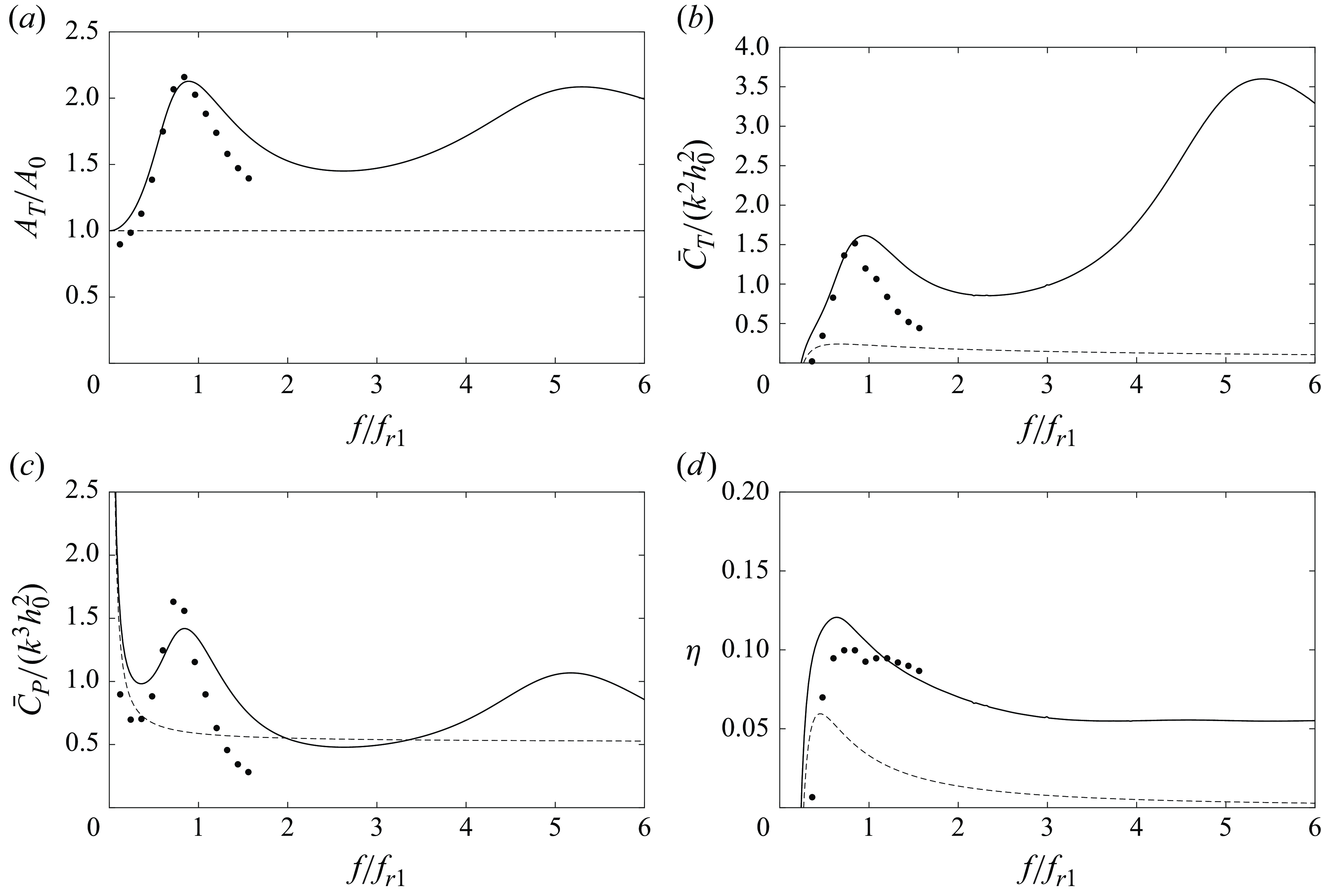
Figure 6. Comparison between the present theoretical results (continuous lines) for $A_T/A_0$
(a),
$A_T/A_0$
(a), $\overline {C}_T/(k^2 h_0^2)$
(b),
$\overline {C}_T/(k^2 h_0^2)$
(b), $\overline {C}_P/(k^3 h_0^2)$
(c) and
$\overline {C}_P/(k^3 h_0^2)$
(c) and $\eta$
(d) with experimental data (symbols) by Quinn, Lauder & Smits (Reference Quinn, Lauder and Smits2014) for a flexible heaving foil with
$\eta$
(d) with experimental data (symbols) by Quinn, Lauder & Smits (Reference Quinn, Lauder and Smits2014) for a flexible heaving foil with $h_0 \simeq 0.1$
. The experimental data are extracted from figure 9 of Paraz et al. (Reference Paraz, Schouveiler and Eloy2016). Dashed lines correspond to the results for the rigid foil counterpart.
$h_0 \simeq 0.1$
. The experimental data are extracted from figure 9 of Paraz et al. (Reference Paraz, Schouveiler and Eloy2016). Dashed lines correspond to the results for the rigid foil counterpart.
Figure 7. Comparison between the present theoretical results for $\overline {C}_T/(k^2 h_0^2)$
at two high values of
$\overline {C}_T/(k^2 h_0^2)$
at two high values of $S$
(continuous lines) with experimental data (symbols) by Paraz et al. (Reference Paraz, Schouveiler and Eloy2016) for a flexible heaving foil with
$S$
(continuous lines) with experimental data (symbols) by Paraz et al. (Reference Paraz, Schouveiler and Eloy2016) for a flexible heaving foil with $h_0 = 0.07$
.
$h_0 = 0.07$
.
The experimental results plotted in figure 6 do not reach frequencies around the second natural mode. Paraz et al. (Reference Paraz, Schouveiler and Eloy2016) report some experimental measurements of the thrust force for higher frequencies in their figure 8(a), but they are made ‘in water at rest’, which represents a difficulty for comparison with current theoretical results because $U$
is used here to make dimensionless
$U$
is used here to make dimensionless $\overline {C}_T$
,
$\overline {C}_T$
, $k$
and
$k$
and $S$
. Formally, their experimental data corresponds to
$S$
. Formally, their experimental data corresponds to $S \to \infty$
and, since these authors report results for
$S \to \infty$
and, since these authors report results for $\overline {C}_T/( k^2 h_0^2)$
in the present notation, in whose non-dimensionalization does not intervene
$\overline {C}_T/( k^2 h_0^2)$
in the present notation, in whose non-dimensionalization does not intervene $U$
, figure 6 compares the experimental data for the case
$U$
, figure 6 compares the experimental data for the case $h_0=0.07$
with the present theoretical results for two large values of the stiffness,
$h_0=0.07$
with the present theoretical results for two large values of the stiffness, $S=5 \times 10^3$
and
$S=5 \times 10^3$
and $S=10^4$
. The mass ratio used is
$S=10^4$
. The mass ratio used is $R=0.16$
, that coincides with that in figure 4, and the same values of the drag coefficients
$R=0.16$
, that coincides with that in figure 4, and the same values of the drag coefficients $C_{Dz}$
and
$C_{Dz}$
and $C_{Dx}$
of the previous comparison are used. The present results underestimate the thrust around the first natural frequency and overestimate it around the second. But taking into account that the limit
$C_{Dx}$
of the previous comparison are used. The present results underestimate the thrust around the first natural frequency and overestimate it around the second. But taking into account that the limit $U=0$
cannot be well captured by the present theoretical approximation, the agreement is not that bad, reproducing correctly the two thrust peaks near the first two natural frequencies. It should also be noted that the thrust is scaled with
$U=0$
cannot be well captured by the present theoretical approximation, the agreement is not that bad, reproducing correctly the two thrust peaks near the first two natural frequencies. It should also be noted that the thrust is scaled with $k^2$
in figure 7, so that the greatest thrust peak really happens around the second mode.
$k^2$
in figure 7, so that the greatest thrust peak really happens around the second mode.
All the other experimental data found by the author in the literature for frequencies near the second natural mode are for large oscillation amplitudes, or for a foil with small aspect ratio, or both, so that the present theory could not be applied.
Figure 8. Normalized flexural deflection amplitude at the trailing edge (a), thrust (b), power (c) and efficiency (d) for pure heave as $k$
and
$k$
and $S$
are varied when
$S$
are varied when $R=0.1$
. Here
$R=0.1$
. Here $C_{Dz}=12$
and
$C_{Dz}=12$
and $C_{Dx}=0.05$
. The vertical dashed line marks the case depicted in figure 6. For the other lines related to the natural frequencies see caption of figure 2.
$C_{Dx}=0.05$
. The vertical dashed line marks the case depicted in figure 6. For the other lines related to the natural frequencies see caption of figure 2.
6. Results and discussion
6.1. Heaving
Figure 8 shows the present theoretical results for the same values of $R$
and
$R$
and $h_0$
considered in figure 6, but for a wide range of the stiffness parameter. The value of
$h_0$
considered in figure 6, but for a wide range of the stiffness parameter. The value of $S$
used for the comparison with experimental data in figure 6 is marked with a white dashed line (note that
$S$
used for the comparison with experimental data in figure 6 is marked with a white dashed line (note that $\overline {C}_T$
and
$\overline {C}_T$
and $\overline {C}_P$
are normalized in figure 6 with
$\overline {C}_P$
are normalized in figure 6 with $k^2h_0^2$
and
$k^2h_0^2$
and $k^3h_0^2$
, respectively, which is not done in figures 8
b and 8
d). Though the largest thrust for this value of the stiffness (
$k^3h_0^2$
, respectively, which is not done in figures 8
b and 8
d). Though the largest thrust for this value of the stiffness ( $S=1269$
) is reached close to the second natural frequency, the power also presents a maximum value there, so that the largest efficiency is obtained near to the first natural frequency, as it is more clearly observed in figure 6.
$S=1269$
) is reached close to the second natural frequency, the power also presents a maximum value there, so that the largest efficiency is obtained near to the first natural frequency, as it is more clearly observed in figure 6.
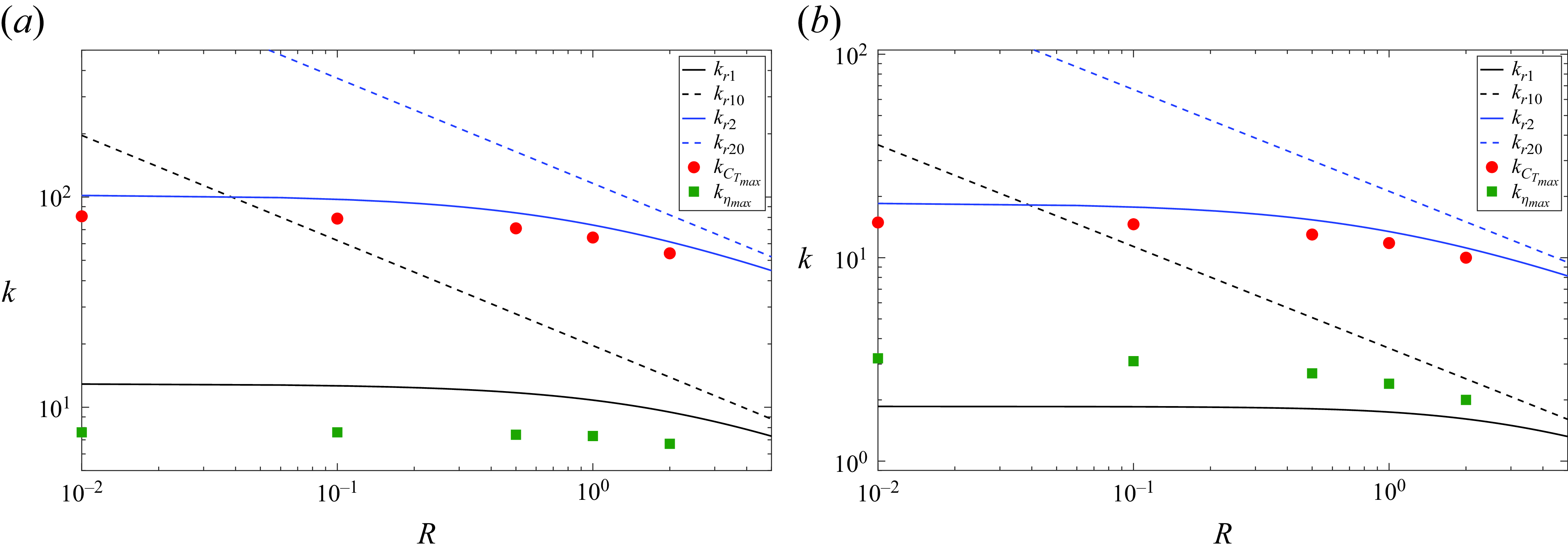
Figure 9. Evolution of the frequencies for $\eta _{max}$
(squares) and
$\eta _{max}$
(squares) and $\overline {C}_{T_{max}}$
(circles) with the mass ratio
$\overline {C}_{T_{max}}$
(circles) with the mass ratio $R$
, for a heaving foil with
$R$
, for a heaving foil with $S=1500$
(a) and
$S=1500$
(a) and $S=50$
(b). For reference, the different lines represent the first and second natural frequencies, as indicated.
$S=50$
(b). For reference, the different lines represent the first and second natural frequencies, as indicated.
As the stiffness decreases, this behaviour remains qualitatively the same, increasing the propulsion efficiency until reaching a peak of approximately $50\, \%$
for
$50\, \%$
for $S \approx 30$
and for a frequency quite above the corresponding first natural frequency (for
$S \approx 30$
and for a frequency quite above the corresponding first natural frequency (for $k \simeq 2.75$
).
$k \simeq 2.75$
).
The model predicts that the propulsive performance improves slightly with the mass ratio $R$
, with a pattern similar to that of figure 8: the highest efficiency around
$R$
, with a pattern similar to that of figure 8: the highest efficiency around $k_{r1}$
for large
$k_{r1}$
for large $S$
, but moving to frequencies in between the two natural modes as
$S$
, but moving to frequencies in between the two natural modes as $S$
decreases. This is better appreciated in figure 9, where the evolutions of the frequencies for the maximum efficiency and the maximum thrust coefficient as
$S$
decreases. This is better appreciated in figure 9, where the evolutions of the frequencies for the maximum efficiency and the maximum thrust coefficient as $R$
is varied are plotted for
$R$
is varied are plotted for $S=1500$
and
$S=1500$
and $S=50$
. The maximum thrust is reached slightly below the second natural frequency, while the maximum efficiency is obtained for frequencies just below the first natural frequency for sufficiently rigid foils, and for frequencies higher than that of the first mode for more flexible foils. In general, both
$S=50$
. The maximum thrust is reached slightly below the second natural frequency, while the maximum efficiency is obtained for frequencies just below the first natural frequency for sufficiently rigid foils, and for frequencies higher than that of the first mode for more flexible foils. In general, both $\overline {C}_{T_{max}}$
and
$\overline {C}_{T_{max}}$
and $\eta _{max}$
increase with the mass ratio
$\eta _{max}$
increase with the mass ratio $R$
.
$R$
.
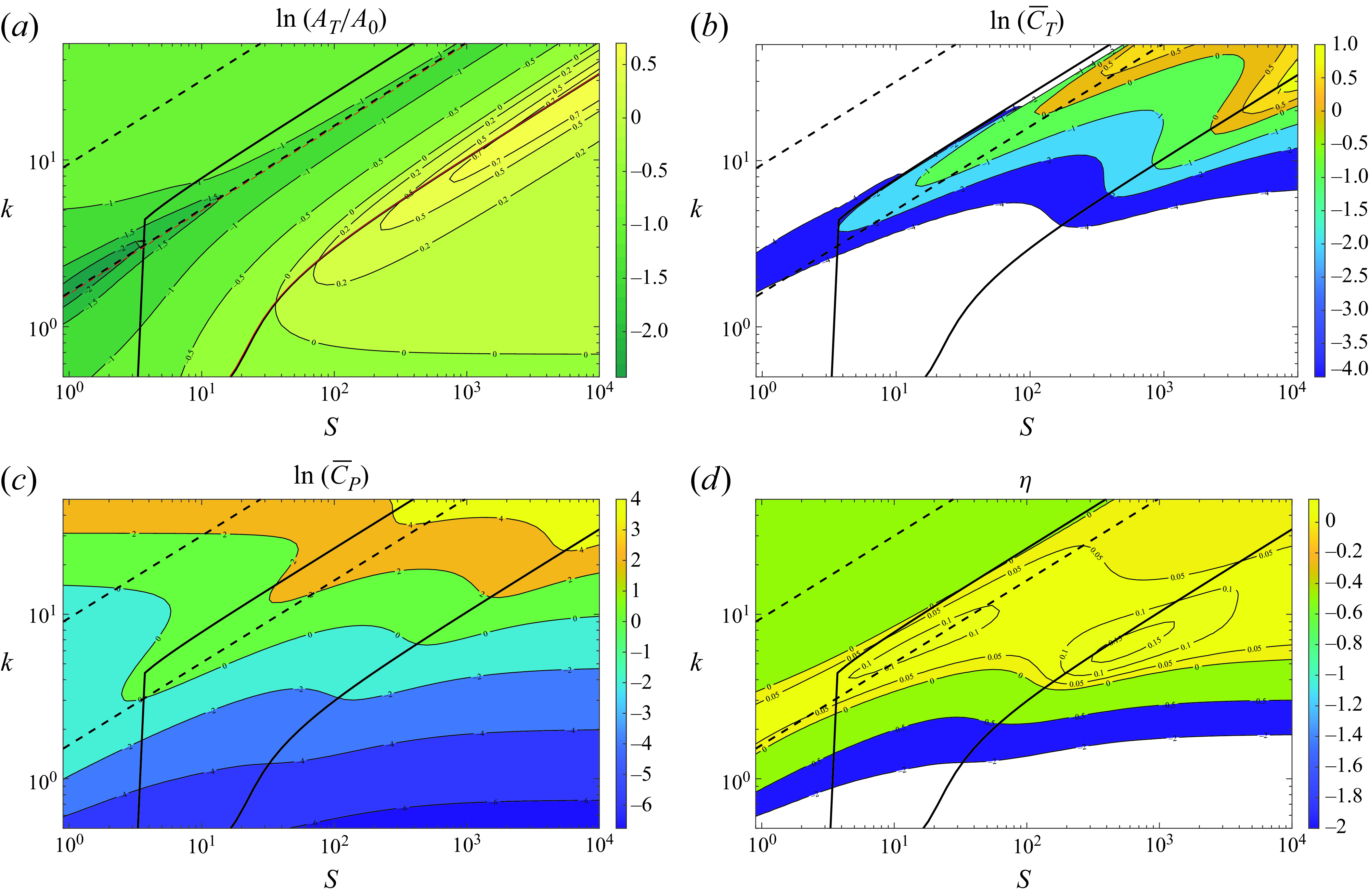
Figure 10. Normalized flexural deflection amplitude at the trailing edge (a), thrust (b), power (c) and efficiency (d) for a pitching foil with $\alpha _0=2^\circ$
and
$\alpha _0=2^\circ$
and $R=0.1$
as
$R=0.1$
as $k$
and
$k$
and $S$
are varied. Here
$S$
are varied. Here $C_{Dz}=12$
and
$C_{Dz}=12$
and $C_{Dx}=0.0373$
. For the lines related to the natural frequencies see caption of figure 2.
$C_{Dx}=0.0373$
. For the lines related to the natural frequencies see caption of figure 2.
6.2. Pitching
For a flexible pitching foil the propulsion pattern when $S$
and
$S$
and $k$
vary is different from that of a heaving foil, as shown in figure 10 for
$k$
vary is different from that of a heaving foil, as shown in figure 10 for $\alpha _0=2^\circ$
and
$\alpha _0=2^\circ$
and $R=0.1$
. The offset viscous drag selected in the computations of figure is
$R=0.1$
. The offset viscous drag selected in the computations of figure is $C_{Dx}=0.0373$
, according to the experimental value given by Mackowski & Williamson (Reference Mackowski and Williamson2015) for this pitching amplitude, whereas
$C_{Dx}=0.0373$
, according to the experimental value given by Mackowski & Williamson (Reference Mackowski and Williamson2015) for this pitching amplitude, whereas $C_{Dz}=12$
as in the previous cases.
$C_{Dz}=12$
as in the previous cases.
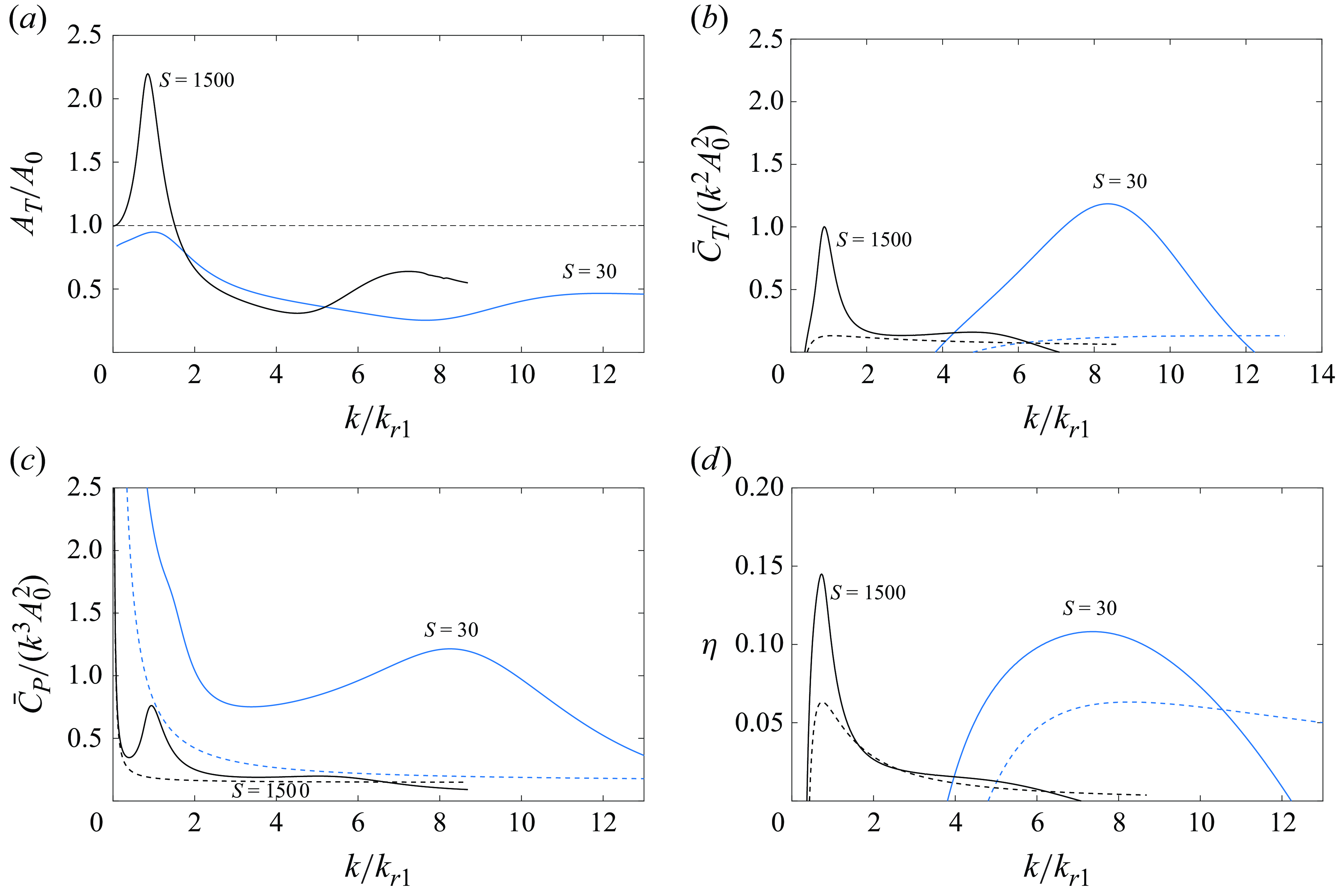
Figure 11. Profiles of $A_T/A_0$
(a),
$A_T/A_0$
(a), $\overline {C}_T/(k^2 A_0^2)$
(b),
$\overline {C}_T/(k^2 A_0^2)$
(b), $\overline {C}_P/(k^3 A_0^2)$
(c), and
$\overline {C}_P/(k^3 A_0^2)$
(c), and $\eta$
(d) versus
$\eta$
(d) versus $k/k_{r1}$
for a flexible pitching foil with
$k/k_{r1}$
for a flexible pitching foil with $\alpha _0=2^\circ$
and
$\alpha _0=2^\circ$
and $R=0.1$
, for
$R=0.1$
, for $S=30$
(blue lines) and
$S=30$
(blue lines) and $S=1500$
(black lines). Dashed lines correspond to the results for the rigid foil counterparts.
$S=1500$
(black lines). Dashed lines correspond to the results for the rigid foil counterparts.
To begin with, figure 10(a) shows that there is no trailing-edge deflection peak at the second natural frequency. Actually, for low stiffnesses, the trailing-edge flexural deflection amplitude is below that of the rigid foil counterpart for all the frequencies, as it is better appreciated in figure 11(a), where two profiles of $A_T/A_0$
versus
$A_T/A_0$
versus $k$
are plotted for
$k$
are plotted for $S=30$
and
$S=30$
and $S=1500$
. Nonetheless, these low-stiffness pitching foils show marked thrust and power peaks around the second natural frequency (see figure 10
b,c and figure 11 for
$S=1500$
. Nonetheless, these low-stiffness pitching foils show marked thrust and power peaks around the second natural frequency (see figure 10
b,c and figure 11 for $S=30$
), whereas for large stiffnesses, the highest peaks of
$S=30$
), whereas for large stiffnesses, the highest peaks of $\overline {C}_T$
and
$\overline {C}_T$
and $\overline {C}_P$
are close to the first natural frequency, which is better appreciated in figures 11(c) and 11(d) for
$\overline {C}_P$
are close to the first natural frequency, which is better appreciated in figures 11(c) and 11(d) for $S=1500$
. As a consequence, the propulsive efficiency pattern is quite different from that of a pure heaving foil (compare figures 10
d and 11
d with figures 8
d and 6
d, respectively): for large and moderate stiffnesses the highest efficiencies are around the first natural frequency, whereas, for lower stiffnesses, pitching foils actuated at the second natural frequency show larger propulsive efficiencies than when actuated at the first one. Actually, according to the present results, a pitching foil with high flexibility only generates thrust when the frequency is around the second natural frequency.
$S=1500$
. As a consequence, the propulsive efficiency pattern is quite different from that of a pure heaving foil (compare figures 10
d and 11
d with figures 8
d and 6
d, respectively): for large and moderate stiffnesses the highest efficiencies are around the first natural frequency, whereas, for lower stiffnesses, pitching foils actuated at the second natural frequency show larger propulsive efficiencies than when actuated at the first one. Actually, according to the present results, a pitching foil with high flexibility only generates thrust when the frequency is around the second natural frequency.
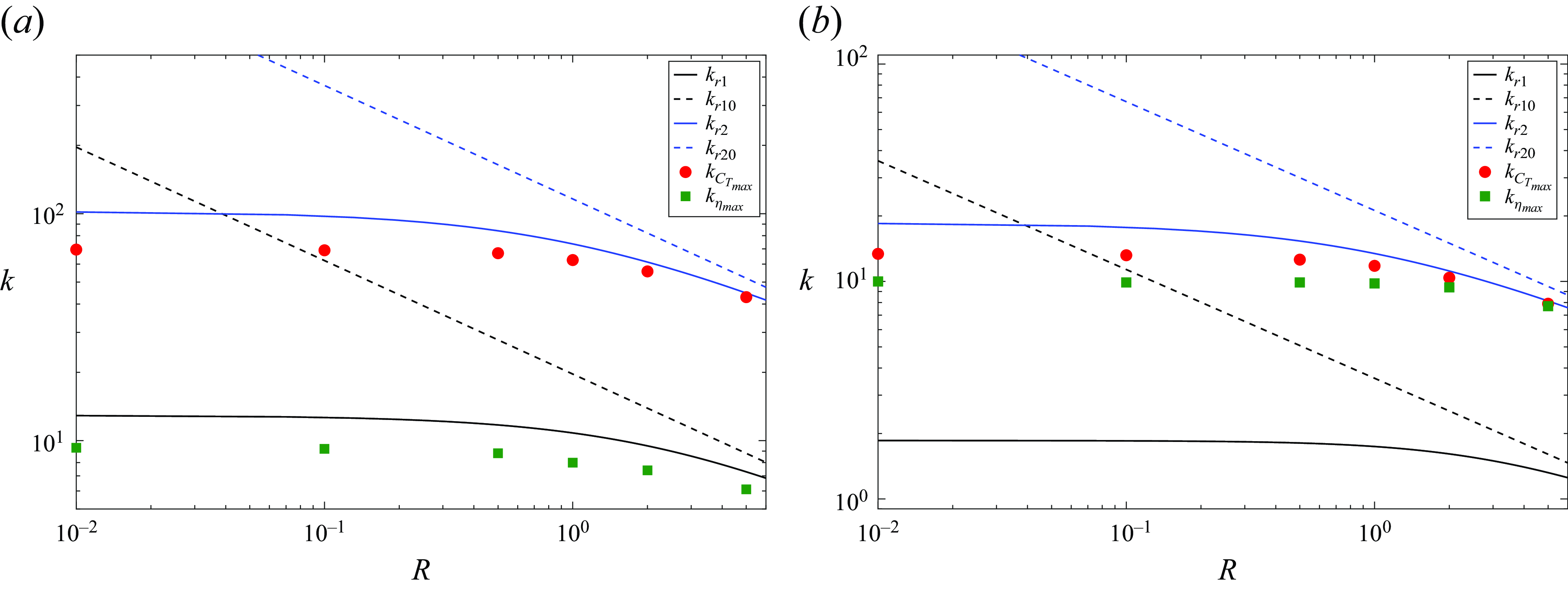
Figure 12. Evolution of the frequencies for $\eta _{max}$
(squares) and
$\eta _{max}$
(squares) and $\overline {C}_{T_{max}}$
(circles) with the mass ratio
$\overline {C}_{T_{max}}$
(circles) with the mass ratio $R$
, for a pitching foil with
$R$
, for a pitching foil with $S=1500$
(a) and
$S=1500$
(a) and $S=50$
(b). The different lines represent the first and second natural frequencies, as indicated.
$S=50$
(b). The different lines represent the first and second natural frequencies, as indicated.
The propulsion pattern for a mass ratio $R=0.1$
shown in figures 10 and 11 remains qualitatively the same for other values of
$R=0.1$
shown in figures 10 and 11 remains qualitatively the same for other values of $R$
, as shown in figure 12. For high stiffnesses, the largest thrust is always reached slightly below the second natural frequency, whereas the maximum efficiency is obtained for frequencies slightly below the first natural frequency (figure 12
a). For more flexible foils, both maxima are attained at practically the same frequencies, below the second mode (figure 12
b).
$R$
, as shown in figure 12. For high stiffnesses, the largest thrust is always reached slightly below the second natural frequency, whereas the maximum efficiency is obtained for frequencies slightly below the first natural frequency (figure 12
a). For more flexible foils, both maxima are attained at practically the same frequencies, below the second mode (figure 12
b).
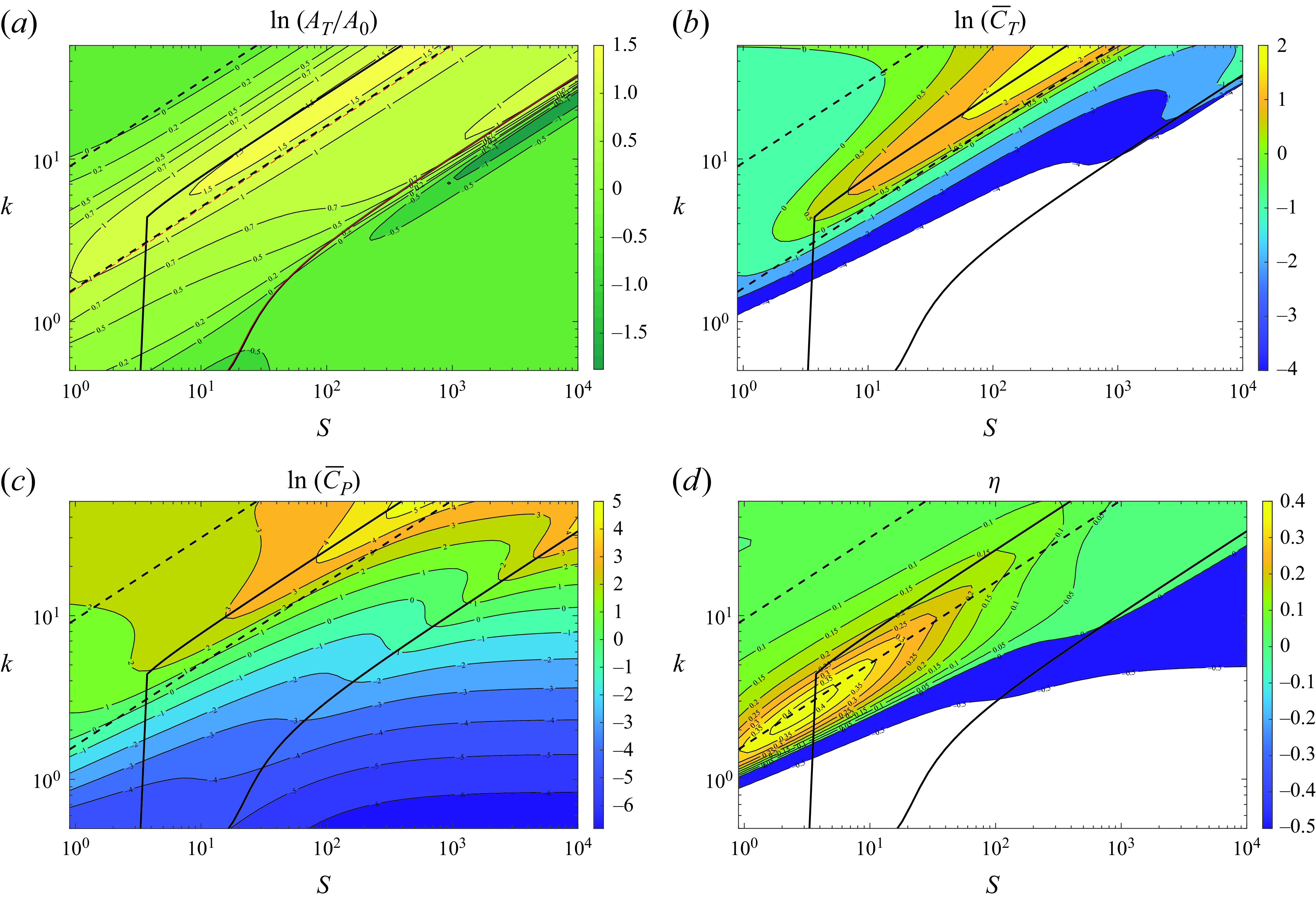
Figure 13. Here $A_T/A_0$
(a),
$A_T/A_0$
(a), $\overline {C}_T$
(b),
$\overline {C}_T$
(b), $\overline {C}_P$
(c) and
$\overline {C}_P$
(c) and $\eta$
(d) for a pitching and heaving foil with
$\eta$
(d) for a pitching and heaving foil with $\alpha _0=2^\circ$
,
$\alpha _0=2^\circ$
, $h_0=0.05$
,
$h_0=0.05$
, $\phi =0$
and
$\phi =0$
and $R=0.1$
as
$R=0.1$
as $k$
and
$k$
and $S$
are varied. Here
$S$
are varied. Here $C_{Dz}=12$
and
$C_{Dz}=12$
and $C_{Dx}=0.05$
.
$C_{Dx}=0.05$
.
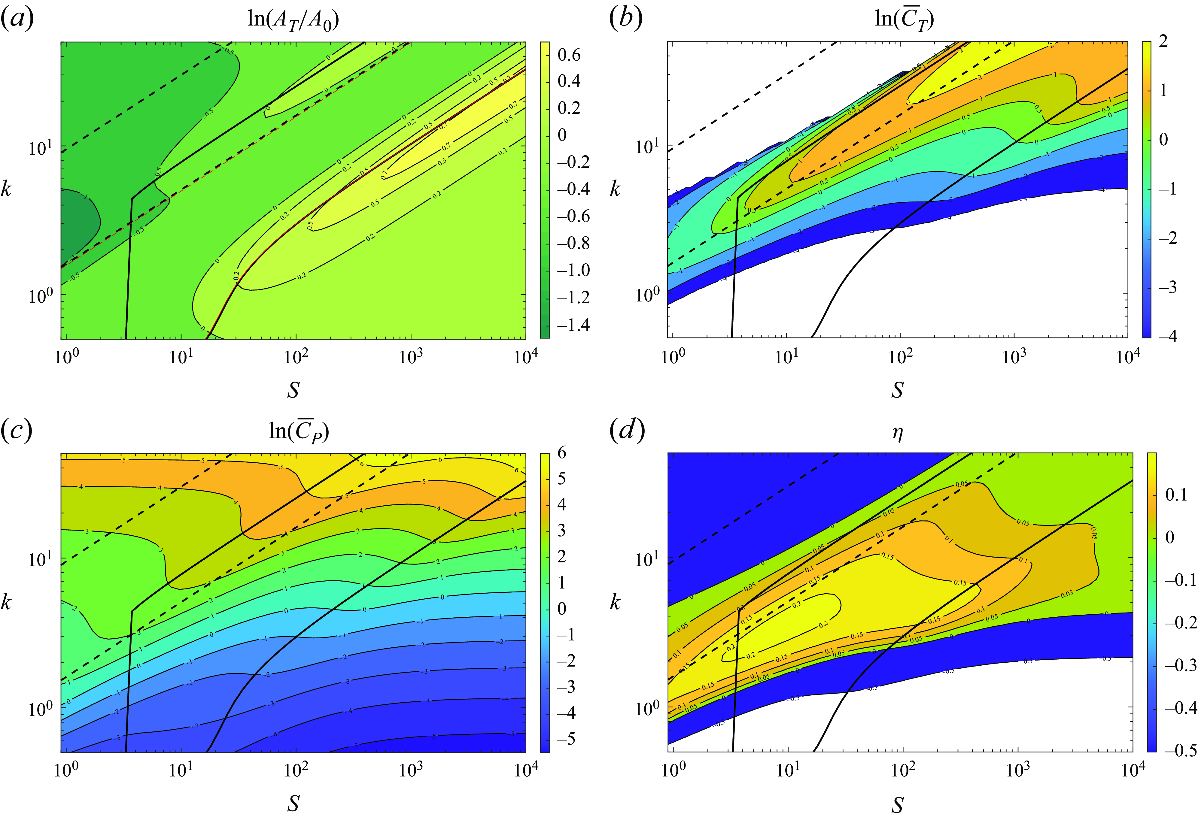
Figure 14. As figure 13 but for $\phi =-90^\circ$
.
$\phi =-90^\circ$
.
6.3. Pitching and heaving
Figures 13 and 14 show the results for a combined pitching and heaving motion with $a_0=2^\circ$
and
$a_0=2^\circ$
and $h_0=0.05$
, both with a mass ratio
$h_0=0.05$
, both with a mass ratio $R=0.1$
. In figure 13 without phase shift (
$R=0.1$
. In figure 13 without phase shift ( $\phi =0$
) and in figure 14 when pitch lags heave by
$\phi =0$
) and in figure 14 when pitch lags heave by $\phi =-90^\circ$
, which approximately corresponds to the rigid foil kinematics with the highest efficiency (Lighthill Reference Lighthill1970; Wu Reference Wu1971a
). Drag coefficients
$\phi =-90^\circ$
, which approximately corresponds to the rigid foil kinematics with the highest efficiency (Lighthill Reference Lighthill1970; Wu Reference Wu1971a
). Drag coefficients $C_{Dz}=12$
and
$C_{Dz}=12$
and $C_{Dx}=0.05$
are used.
$C_{Dx}=0.05$
are used.
In both cases the flexural deflection has peaks around the two natural frequencies if the stiffness is high enough. But, when heave and pitch are in phase (figure 13
a) the local maximum of $A_T/A_0$
around the first natural mode is very weak, whereas it is almost suppressed about the second one for
$A_T/A_0$
around the first natural mode is very weak, whereas it is almost suppressed about the second one for $\phi =-90^\circ$
(figure 14
a). Despite these differences, the largest thrust is always generated around the second mode for large stiffnesses (figures 13
b and 14
b), which also needs the largest input power (figures 13
c and 14
c), so that the largest efficiency is not reached near neither of these natural frequencies for large stiffnesses. Only for
$\phi =-90^\circ$
(figure 14
a). Despite these differences, the largest thrust is always generated around the second mode for large stiffnesses (figures 13
b and 14
b), which also needs the largest input power (figures 13
c and 14
c), so that the largest efficiency is not reached near neither of these natural frequencies for large stiffnesses. Only for $\phi =0$
there is a local maximum of
$\phi =0$
there is a local maximum of $\eta$
around
$\eta$
around $k_{r2}$
for large
$k_{r2}$
for large $S$
(figure 13
d). The largest efficiency is reached in both cases for
$S$
(figure 13
d). The largest efficiency is reached in both cases for $S$
of order
$S$
of order $10$
or below (recall that the present theory fails as
$10$
or below (recall that the present theory fails as $S$
becomes of order unity, when the two natural frequencies merge). It is close to (but clearly below) the second mode for
$S$
becomes of order unity, when the two natural frequencies merge). It is close to (but clearly below) the second mode for $\phi =0$
, which presents the largest efficiency, while for
$\phi =0$
, which presents the largest efficiency, while for $\phi =-90^\circ$
the highest efficient is not related to the resonant frequencies (figure 14
d).
$\phi =-90^\circ$
the highest efficient is not related to the resonant frequencies (figure 14
d).
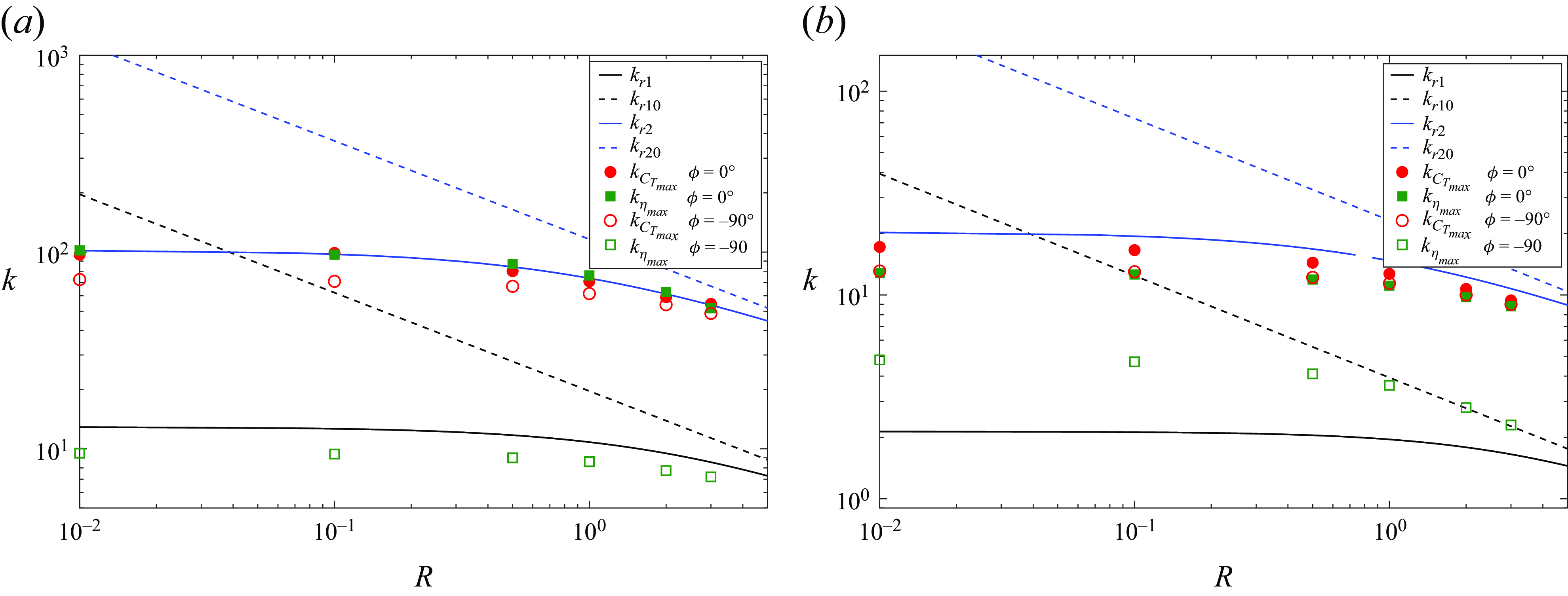
Figure 15. Evolution of the frequencies for $\eta _{max}$
(squares) and
$\eta _{max}$
(squares) and $\overline {C}_{T_{max}}$
(circles) with the mass ratio
$\overline {C}_{T_{max}}$
(circles) with the mass ratio $R$
, for a pitching and heaving foil (
$R$
, for a pitching and heaving foil ( $a_0=2^\circ$
and
$a_0=2^\circ$
and $h_0=0.05$
) with
$h_0=0.05$
) with $S=1500$
(a) and
$S=1500$
(a) and $S=50$
(b) for
$S=50$
(b) for $\phi =0^\circ$
(filled symbols) and
$\phi =0^\circ$
(filled symbols) and $\phi =-90^\circ$
(open symbols). The different lines represent the first and second natural frequencies, as indicated.
$\phi =-90^\circ$
(open symbols). The different lines represent the first and second natural frequencies, as indicated.
As shown in figure 15, these propulsion patterns for $R=0.1$
remain qualitatively the same as
$R=0.1$
remain qualitatively the same as $R$
is varied. For large stiffness (figure 15
a) and
$R$
is varied. For large stiffness (figure 15
a) and $\phi =0$
, both
$\phi =0$
, both $\overline {C}_{T_{max}}$
and
$\overline {C}_{T_{max}}$
and $\eta _{max}$
are obtained practically at the second natural frequency, whereas for
$\eta _{max}$
are obtained practically at the second natural frequency, whereas for $\phi =-90^\circ$
, the maximum thrust is generated for a frequency below
$\phi =-90^\circ$
, the maximum thrust is generated for a frequency below $k_{r2}$
and the maximum propulsive efficiency for frequencies lower than the first natural frequency. For more flexible foils (figure 15
b), the main difference is that the maximum propulsive efficiency when
$k_{r2}$
and the maximum propulsive efficiency for frequencies lower than the first natural frequency. For more flexible foils (figure 15
b), the main difference is that the maximum propulsive efficiency when $\phi =-90^\circ$
is obtained for frequencies in between the two natural frequencies, with no apparent relation to any of them. Both
$\phi =-90^\circ$
is obtained for frequencies in between the two natural frequencies, with no apparent relation to any of them. Both $\overline {C}_{T_{max}}$
and
$\overline {C}_{T_{max}}$
and $\eta _{max}$
increase with
$\eta _{max}$
increase with $R$
in all the cases considered.
$R$
in all the cases considered.
For other phase shifts different from $\phi =0^\circ$
and
$\phi =0^\circ$
and $\phi =-90^\circ$
the results are found to be very similar to those depicted in figure 13 for
$\phi =-90^\circ$
the results are found to be very similar to those depicted in figure 13 for $\phi$
close to zero or to
$\phi$
close to zero or to $180^\circ$
, whereas the results in figure 14 are representative for any
$180^\circ$
, whereas the results in figure 14 are representative for any $\phi$
around
$\phi$
around $\pm 90^\circ$
. It may be concluded that for large stiffnesses one must operate around the second natural frequency with pitch and heave in phase to obtain the largest thrust and efficiency. Out of phase (for
$\pm 90^\circ$
. It may be concluded that for large stiffnesses one must operate around the second natural frequency with pitch and heave in phase to obtain the largest thrust and efficiency. Out of phase (for $\phi$
around
$\phi$
around $\pm 90^\circ$
), though the largest thrust is still generated close to the second mode, the efficiency is the highest near the first mode. For low stiffness
$\pm 90^\circ$
), though the largest thrust is still generated close to the second mode, the efficiency is the highest near the first mode. For low stiffness $S$
, no relation is found between high efficiencies and resonant frequencies, especially when pitch and heave are out of phase.
$S$
, no relation is found between high efficiencies and resonant frequencies, especially when pitch and heave are out of phase.
7. Conclusion
An analytical formulation of the FSI between a uniform fluid current and a 2-D pitching and heaving flexible plate, which models the interaction up to the first two natural frequencies of the system, is presented in this work, and their results are compared with available experimental data for small-amplitude oscillations. It is based on a fifth-order polynomial profile for the flexible plate, the simplest approximation for the deformation of a thin plate governed by the E–B beam equation that is capable of fulfilling the trailing-edge boundary conditions and capturing the first two resonant frequencies when subjected to an arbitrary pitching and heaving motion about a pivot axis close to the leading edge. The main contribution is the analytical derivation of the force, moment and the first two flexural moments that the inviscid flow exerts on the flexible plate, extending and systematizing previous works, together with the coupling of these expressions with the first four moments of the E–B equation. These equations allow the analytical computation of the dynamic deformation of the foil for a given pitching and heaving motion, along with the power needed to generate this motion which includes the sometimes-ignored effects of the inertia of the plate. The approach is based on the linearized potential flow theory and the E–B beam equation, so that it is limited to small-amplitude oscillations and deformations of the plate. With the fifth-order polynomial approximation this limitation can be met when a nonlinear damping term is included in the E–B equation to cushion the deformation peaks at the two resonant frequencies, especially at the second, after whose correction the deformation shows a good agreement with experimental results for small-amplitude pitch and heave. This approximation is also at the edge between the purely oscillatory behaviour and the undulatory one of the foil. For this last behaviour the present approach based on the moments of the E–B equation would not be possible, so that it wouldn’t be possible or practical to extend this approximation to cover the following natural modes, which are normally obtained numerically from a modal decomposition of the E–B equation, typically with a Chebyshev expansion.
These analytical results may be of interest to analyse easily problems where the knowledge of the FSI of a flexible plate up to the second natural mode is needed. Here it has been applied to the propulsion problem. To that end, the thrust force exerted by the fluid on the pitching and heaving foil whose deformation is approximated by a general fifth-order polynomial has also been obtained analytically in the linearized potential flow limit using the vortex impulse formulation. The derivation extends and systematize previous works. The resulting thrust has also been validated against available experimental data for small-amplitude oscillations of the foil. In general, the results of the present model for the different magnitudes agree better with experimental results for frequencies around the first natural mode than around the second one, with the latter experimental data being much scarcer.
With these two analytical tools, the propulsion performance of a pitching and/or heaving flexible plate actuated at its leading edge with frequencies up to the second natural frequency has been analysed. The maximum thrust generated, and the maximum input power required, are generally achieved with frequencies close to the natural ones, in agreement with some previous works, whereas the maximum propulsive efficiency occurs at frequencies close to that of the first natural mode if the foil is sufficiently rigid, but it is not related to the natural frequencies as the rigidity decreases, being the optimum efficiency somewhere between the two natural modes for low stiffnesses. However, it is found that the propulsion patterns as the stiffness varies are quite different for pitching and for heaving foils. Thus, for instance, it is found that a pitching foil with high flexibility only generates thrust when the frequency is around the second natural frequency, whereas for large and moderate stiffnesses the highest thrust and efficiency are around the first natural frequency, with negligible thrust as the second natural frequency is approached. On the other hand, for heaving foils, the maximum thrust is reached slightly below the second natural frequency, while the maximum efficiency is obtained for frequencies just below the first natural mode for sufficiently rigid foils, and for frequencies higher than that of the first mode for more flexible foils. When pitch and heave are actuated simultaneously, one must operate around the second natural frequency to obtain the largest thrust and efficiency when pitch and heave are phase, whereas, out of phase, the largest thrust is still generated close to the second mode, but the efficiency is the highest near the first mode. For low stiffness, no relation is found between high efficiencies and resonant frequencies, especially when pitch and heave are out of phase. The approach ceases to be valid when the two natural modes provided by the model merge for values of the stiffness parameter of order unity.
Obviously, the present results cannot be extrapolated to cases when the pitch/heave amplitude is not small, or when the plate undergoes deformations of great amplitude, because the separation phenomena would be very important. But even for small amplitudes, the results would not be applicable to low-Reynolds-number flows, when the viscous effects are very relevant and cannot be taken into consideration through simple drags coefficients, or when the aspect ratio of the plate is not sufficiently large, because three-dimensionality effects cannot be disregarded. But, in any case, the formulation provides a useful analytical tool to quickly estimate the behaviour of a small-amplitude oscillating foil immersed in a fluid current.
Funding
This research has been supported by the MCIyU/AEI grant PID2023-150588NB-I00.
Declaration of interests
The author reports no conflict of interest.
Appendix A. Equation (3.1)
The unsteady, linearized Bernoulli equation for the inviscid and incompressible flow on the plate can be written, in non-dimensional form, as
 \begin{equation} \Delta P = \frac {\partial (\Delta \Phi)}{\partial t} + \frac {1}{2} [(u^+)^2 - (u^-)^2] , \end{equation}
where $\Phi$
is the non-dimensional velocity potential (
$\Phi$
is the non-dimensional velocity potential ( $u= \partial \Phi /\partial x$
) and
$u= \partial \Phi /\partial x$
) and $\Delta \Phi = \Phi ^+-\Phi ^-$
, with superscripts
$\Delta \Phi = \Phi ^+-\Phi ^-$
, with superscripts $+$
and
$+$
and $-$
denoting the upper and lower surfaces of the plate, respectively, as defined in the main text (recall that the non-dimensional pressure difference has been defined as
$-$
denoting the upper and lower surfaces of the plate, respectively, as defined in the main text (recall that the non-dimensional pressure difference has been defined as $\Delta P =(p^--p^+)/(\rho U^2)$
). Using the non-dimensional vorticity density distribution on the plate,
$\Delta P =(p^--p^+)/(\rho U^2)$
). Using the non-dimensional vorticity density distribution on the plate, $\varpi _s(x,t) = u^+(x,t) - u^-(x,t)$
, one may write
$\varpi _s(x,t) = u^+(x,t) - u^-(x,t)$
, one may write
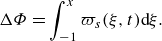 \begin{align} \Delta \Phi = \int _{-1}^x \varpi _s(\xi,t) {\textrm d}\xi . \end{align}
Since $(u^+ + u^-)/2$
is the free stream velocity in the present linearized theory, which is unity in non-dimensional variables, introducing these expressions into (A1) one obtains (3.1).
$(u^+ + u^-)/2$
is the free stream velocity in the present linearized theory, which is unity in non-dimensional variables, introducing these expressions into (A1) one obtains (3.1).
Appendix B. The ${ \mathsf{A}}_{\,\boldsymbol c}$
and
${\boldsymbol {b}}_{\boldsymbol c}$
in (4.15)
${ \mathsf{A}}_{\,\boldsymbol c}$
and
${\boldsymbol {b}}_{\boldsymbol c}$
in (4.15)


Here ${ \mathsf{A}}_c$
and
${ \mathsf{A}}_c$
and ${\boldsymbol {b}}_c$
are given by
${\boldsymbol {b}}_c$
are given by
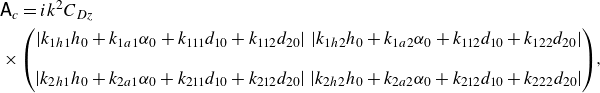 \begin{align} &{ \mathsf{A}}_c = i k^2 C_{Dz} \nonumber \\ &\times \left ( \begin{array}{@{}cc@{}} \left | k_{1h1} h_0+ k_{1a1} \alpha _0 + k_{111} d_{10}+k_{112} d_{20} \right | & \left | k_{1h2} h_0+ k_{1a2} \alpha _0 +k_{112} d_{10}+k_{122} d_{20} \right | \\ \\ \left |k_{2h1} h_0+ k_{2a1} \alpha _0 + k_{211} d_{10}+k_{212} d_{20} \right | & \left | k_{2h2} h_0+ k_{2a2} \alpha _0 + k_{212} d_{10}+k_{222} d_{20} \right | \end{array} \right)\!, \end{align}
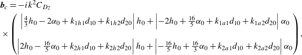 \begin{align} &{\boldsymbol {b}}_c = - i k^2 C_{Dz} \nonumber \\ &\times\left ( \begin{array}{@{}c@{}} \left | \frac {4}{3} h_0 -2 \alpha _0 + k_{1h1} d_{10}+k_{1h2} d_{20} \right | h_0 + \left | -2 h_0+ \frac {16}{5} \alpha _0 +k_{1a1} d_{10}+k_{1a2} d_{20} \right | \alpha _0 \\ \\ \left | 2 h_0 -\frac {16}{5} \alpha _0 + k_{2h1} d_{10}+k_{2h2} d_{20} \right |h_0 + \left | - \frac {16}{5} h_0+ \frac {16}{3} \alpha _0 + k_{2a1} d_{10}+k_{2a2} d_{20} \right | \alpha _0 \end{array} \right)\!, \end{align}
where the $k_{\ldots }\hbox{-}$
coefficients are given by
$k_{\ldots }\hbox{-}$
coefficients are given by
 \begin{align} k_{1h1}=\frac {4544}{105} \,, \quad k_{1h2}=\frac {944}{3} \,, \quad k_{1a1}=-\frac {496}{7} \,, \quad k_{1a2}=-\frac {32512}{63} \,, \end{align}
 \begin{align} k_{2h1}=\frac {496}{7} \,, \quad k_{2h2}=\frac {32512}{63} \,, \quad k_{2a1}=-\frac {7552}{63} \,, \quad k_{2a2}=-\frac {30592}{35} \,, \end{align}
 \begin{align} k_{111}=\frac {5481472}{3465} \,, \quad k_{112}=\frac {4438528}{385} \,, \quad k_{122}=\frac {756936704}{9009} \,, \end{align}
 \begin{align} k_{211}=\frac {148992}{55} \,, \quad k_{212}=\frac {25432064}{1287} \,, \quad k_{222}=\frac {99897344}{693} \,. \end{align}
Appendix C. Functions
$\boldsymbol{\Gamma _{\ldots } (t)}$
and
$\boldsymbol{\Gamma _{0 \ldots }(t)}$
in (5.6) and (5.15)


The functions $\Gamma _{a} (t)$
,
$\Gamma _{a} (t)$
, $\Gamma _{d_1} (t)$
and
$\Gamma _{d_1} (t)$
and $\Gamma _{d_2} (t)$
appearing in (5.6) are
$\Gamma _{d_2} (t)$
appearing in (5.6) are
 \begin{equation} \Gamma _a(t)= - \frac {\pi }{8} \left [ 8 (\alpha -\dot {h}) + 16 \dot {\alpha } - 272 d_1 - 377 \dot {d}_1 - 2045 d_2 - 2758 \dot {d}_2 \right]\!, \end{equation}
 \begin{equation} \Gamma _{d_1}(t)= \frac {\pi }{64} \left [ 1008 (\alpha -\dot {h})+ 2200 \dot {\alpha } - 35172 d_1 - 53138 \dot {d}_1 - 265410 d_2 - 389427 \dot {d}_2 \right]\!, \end{equation}
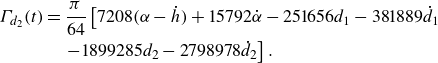 \begin{align}\nonumber \Gamma _{d_2}(t) &= \frac {\pi }{64} \left [ 7208 (\alpha -\dot {h})+ 15792 \dot {\alpha } - 251656 d_1 - 381889 \dot {d}_1 \right. \\ & \left. \quad - 1899285 d_2 - 2798978 \dot {d}_2 \right] . \end{align}
The different functions $\Gamma _{0 \ldots }(t)$
appearing in (5.15) are defined in terms of
$\Gamma _{0 \ldots }(t)$
appearing in (5.15) are defined in terms of $\Gamma _0(t)$
(3.15) and the above functions as
$\Gamma _0(t)$
(3.15) and the above functions as
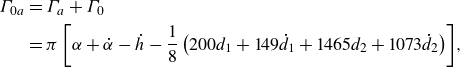 \begin{align} \Gamma _{0a} & = \Gamma _a + \Gamma _0 \nonumber \\ &= \pi \left [ \alpha + \dot {\alpha }-\dot {h} - \frac {1}{8} \left ( 200 d_1+149 \dot {d}_1+1465 d_2+1073 \dot {d}_2 \right) \right]\!, \end{align}
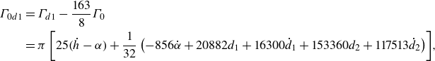 \begin{align} \Gamma _{0d1} &= \Gamma _{d1} - \frac {163}{8} \Gamma _0 \nonumber \\ &= \pi \left [ 25 ( \dot {h} - \alpha) + \frac {1}{32} \left ( - 856 \dot {\alpha } +20882 d_1+16300 \dot {d}_1+153360 d_2+117513 \dot {d}_2 \right) \right]\!, \end{align}
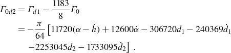 \begin{align} \Gamma _{0d2} &= \Gamma _{d1} - \frac {1183}{8} \Gamma _0 \nonumber \\ &= - \frac {\pi }{64} \left[ 11720 ( \alpha - \dot {h}) + 12600 \dot {\alpha } -306720 d_1-240369 \dot {d}_1 \right.\nonumber \\ &\left.\quad -2253045 d_2- 1733095\dot {d}_2 \right] \,. \end{align}
Appendix D. Functions
$\boldsymbol{\mathcal{C}}_{\ldots }(\boldsymbol{k})$
in (5.16)

In addition to the well-known Theodorsen function $\mathcal{C}(k)$
, defined in (3.14) and appearing in the circulatory parts of the lift and the other moment coefficients obtained in § 3, some other complex functions of the reduced frequency
$\mathcal{C}(k)$
, defined in (3.14) and appearing in the circulatory parts of the lift and the other moment coefficients obtained in § 3, some other complex functions of the reduced frequency $k$
appear in the circulatory part (5.16) of the thrust coefficient. They are defined as the following integrals involving the
$k$
appear in the circulatory part (5.16) of the thrust coefficient. They are defined as the following integrals involving the $k\hbox{-}$
dependence of the wake vorticity distribution (5.13):
$k\hbox{-}$
dependence of the wake vorticity distribution (5.13):
 \begin{equation} \mathcal{C}_h(k) = \mathcal{H}(k) \int _1^\infty e^{- i k \xi } {\textrm d}{\xi} , \end{equation}
 \begin{equation} \mathcal{C}_{a1}(k) = \mathcal{H}(k) \int _1^\infty I_a(\xi) e^{- i k \xi } {\textrm d}{\xi} = \mathcal{H}(k) \int _1^\infty (\sqrt {\xi ^2-1}-\xi) e^{- i k \xi } {\textrm d}{\xi} , \end{equation}
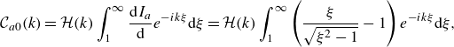 \begin{equation} \mathcal{C}_{a0}(k) = \mathcal{H}(k) \int _1^\infty \frac {{\textrm d} I_a}{{\textrm d}} e^{- i k \xi } {\textrm d}{\xi} = \mathcal{H}(k) \int _1^\infty \left ( \frac {\xi }{\sqrt {\xi ^2-1}} - 1 \right) e^{- i k \xi } {\textrm d}{\xi} , \end{equation}
 \begin{equation} \mathcal{C}_{d11}(k) = -\mathcal{H}(k) \int _1^\infty I_{d1}(\xi) e^{- i k \xi } {\textrm d}{\xi}, \end{equation}
 \begin{equation} \mathcal{C}_{d10}(k) = -\mathcal{H}(k) \int _1^\infty \frac {{\textrm d} I_{d1}}{{\textrm d}{\xi} } e^{- i k \xi } {\textrm d}{\xi} , \end{equation}
 \begin{equation} \mathcal{C}_{d21}(k) = -\mathcal{H}(k) \int _1^\infty I_{d2}(\xi) e^{- i k \xi } {\textrm d}{\xi}, \end{equation}
 \begin{equation} \mathcal{C}_{d20}(k) = -\mathcal{H}(k) \int _1^\infty \frac {{\textrm d} I_{d2}}{{\textrm d}{\xi} } e^{- i k \xi } {\textrm d}{\xi} , \end{equation}
where $\mathcal{H}(k)$
is defined in (5.13) and
$\mathcal{H}(k)$
is defined in (5.13) and $I_a(\xi)$
,
$I_a(\xi)$
, $I_{d1}(\xi)$
and
$I_{d1}(\xi)$
and $I_{d2}(\xi)$
in (5.8)–(5.10).
$I_{d2}(\xi)$
in (5.8)–(5.10).
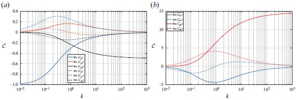
Figure 16. Real and imaginary parts of the functions $\mathcal{C}_{\ldots }(k)$
.
$\mathcal{C}_{\ldots }(k)$
.
The first three ones can easily be obtained analytically (von Kármán & Sears Reference von Kármán and Sears1938; Fernandez-Feria Reference Fernandez-Feria2016; Alaminos-Quesada & Fernandez-Feria Reference Alaminos-Quesada and Fernandez-Feria2020),
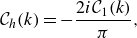 \begin{equation} \mathcal{C}_h(k)= - \frac {2 i \mathcal{C}_1(k)}{\pi } , \end{equation}
 \begin{equation} \mathcal{C}_{a1}(k)= \frac {i}{k} \mathcal{C}(k) + \frac {2 (1 + i k)}{\pi k} \mathcal{C}_1(k) , \end{equation}
 \begin{equation} \mathcal{C}_{a0}(k) = - \mathcal{C}(k) + \frac {2 i \mathcal{C}_1(k) }{\pi } , \end{equation}
where $\mathcal{C}(k)$
is Theodorsen’s function (Theodorsen Reference Theodorsen1935), and
$\mathcal{C}(k)$
is Theodorsen’s function (Theodorsen Reference Theodorsen1935), and $\mathcal{C}_1(k)$
, defined in Fernandez-Feria (Reference Fernandez-Feria2016), is
$\mathcal{C}_1(k)$
, defined in Fernandez-Feria (Reference Fernandez-Feria2016), is
 \begin{equation} \mathcal{C}_1(k)= \frac {e^{-ik}/k}{ i H_0^{(2)} (k) + H_1^{(0)}(k) } . \end{equation}
The analytical expressions for the remaining functions (D4)–(D7) are so involved that they are better computed numerically, which is a quite straightforward and quick task. For validation, the numerical integration code for these functions has also been used for $\mathcal{C}_{a1}(k)$
and
$\mathcal{C}_{a1}(k)$
and $\mathcal{C}_{a0}(k)$
, reproducing the analytical expressions (D9)–(D10) with great accuracy. The real and imaginary parts of these later functions are plotted in figure 16(a), whereas those corresponding to the functions
$\mathcal{C}_{a0}(k)$
, reproducing the analytical expressions (D9)–(D10) with great accuracy. The real and imaginary parts of these later functions are plotted in figure 16(a), whereas those corresponding to the functions $\mathcal{C}_{d11}(k)$
and
$\mathcal{C}_{d11}(k)$
and $\mathcal{C}_{d10}(k)$
obtained numerically are plotted in figure 16(b). Functions
$\mathcal{C}_{d10}(k)$
obtained numerically are plotted in figure 16(b). Functions $\mathcal{C}_{d21}(k)$
and
$\mathcal{C}_{d21}(k)$
and $\mathcal{C}_{d20}(k)$
are no represented because they turn out to be related to
$\mathcal{C}_{d20}(k)$
are no represented because they turn out to be related to $\mathcal{C}_{d11}(k)$
and
$\mathcal{C}_{d11}(k)$
and $\mathcal{C}_{d10}(k)$
through
$\mathcal{C}_{d10}(k)$
through
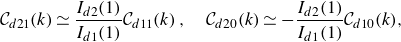 \begin{equation} \mathcal{C}_{d21}(k) \simeq \frac {I_{d2}(1)}{I_{d1}(1)} \mathcal{C}_{d11}(k) \,, \quad \mathcal{C}_{d20}(k) \simeq - \frac {I_{d2}(1)}{I_{d1}(1)} \mathcal{C}_{d10}(k) , \end{equation}
with $I_{d2}(1)/I_{d1}(1)= 1633/221$
(see (5.11)). Note also that
$I_{d2}(1)/I_{d1}(1)= 1633/221$
(see (5.11)). Note also that $\mathrm{Re} [\mathcal{C}_{d11}]=-\mathrm{Im} [\mathcal{C}_{d10}]$
, so that
$\mathrm{Re} [\mathcal{C}_{d11}]=-\mathrm{Im} [\mathcal{C}_{d10}]$
, so that $\mathrm{Re} [\mathcal{C}_{d21}]=\mathrm{Im} [\mathcal{C}_{d20}]$
.
$\mathrm{Re} [\mathcal{C}_{d21}]=\mathrm{Im} [\mathcal{C}_{d20}]$
.
Appendix E. Coefficients of the cycle-averaged thrust (5.18)
In the following expressions for $t_h, t_a, t_{d_1}, t_{d_2}, t_{ha}, t_{hd1}, t_{hd2}, t_{ad1}, t_{ad2}$
and
$t_h, t_a, t_{d_1}, t_{d_2}, t_{ha}, t_{hd1}, t_{hd2}, t_{ad1}, t_{ad2}$
and $t_{d1d2}$
, the functions
$t_{d1d2}$
, the functions $\mathcal{F}_{\ldots }(k)$
and
$\mathcal{F}_{\ldots }(k)$
and $\mathcal{G}_{\ldots }(k)$
are the real and imaginary parts, respectively, of the complex functions
$\mathcal{G}_{\ldots }(k)$
are the real and imaginary parts, respectively, of the complex functions $\mathcal{C}_{\ldots }(k)$
defined in Appendix D; thus, for instance,
$\mathcal{C}_{\ldots }(k)$
defined in Appendix D; thus, for instance, $\mathcal{F}_h(k) = \mathrm{Re} [\mathcal{C}_h(k)]=2G_1(k)/\pi$
and
$\mathcal{F}_h(k) = \mathrm{Re} [\mathcal{C}_h(k)]=2G_1(k)/\pi$
and $\mathcal{G}_h(k)= \mathrm{Im} [\mathcal{C}_h(k)]=-2\mathcal{F}_1/\pi$
(these functions
$\mathcal{G}_h(k)= \mathrm{Im} [\mathcal{C}_h(k)]=-2\mathcal{F}_1/\pi$
(these functions $\mathcal{F}_{\ldots }(k)$
and
$\mathcal{F}_{\ldots }(k)$
and $\mathcal{G}_{\ldots }(k)$
are plotted in figure 16):
$\mathcal{G}_{\ldots }(k)$
are plotted in figure 16):
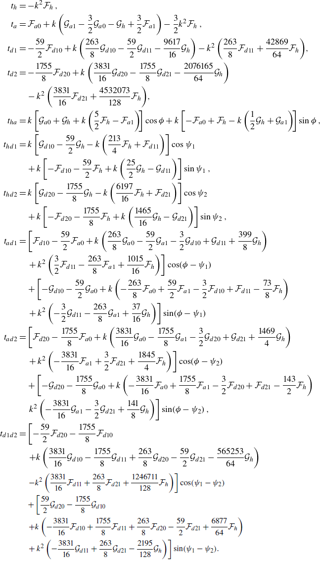 \begin{align} t_h & = - k^2 \mathcal{F}_h \,, \nonumber \\ t_a &= \mathcal{F}_{a0} + k \left ( \mathcal{G}_{a1} - \frac {3}{2} \mathcal{G}_{a0} - \mathcal{G}_h + \frac {3}{2} \mathcal{F}_{a1} \right) - \frac {3}{2} k^2 \mathcal{F}_h \,, \nonumber \\ t_{d1}& = -\frac {59}{2} \mathcal{F}_{d10} + k \left ( \frac {263}{8} \mathcal{G}_{d10} - \frac {59}{2} \mathcal{G}_{d11} - \frac {9617}{16}\mathcal{G}_h \right) - k^2 \left ( \frac {263}{8} \mathcal{F}_{d11} + \frac {42869}{64} \mathcal{F}_h \right)\!, \nonumber \\ t_{d2} &= -\frac {1755}{8} \mathcal{F}_{d20} + k \left ( \frac {3831}{16} \mathcal{G}_{d20} - \frac {1755}{8} \mathcal{G}_{d21} - \frac {2076165}{64}\mathcal{G}_h \right)\nonumber \\ &\quad - k^2 \left ( \frac {3831}{16} \mathcal{F}_{d21} + \frac {4532073}{128} \mathcal{F}_h \right)\!, \nonumber \\ t_{ha} &= k \left [ \mathcal{G}_{a0} + \mathcal{G}_h +k \left ( \frac {5}{2} \mathcal{F}_h - \mathcal{F}_{a1} \right)\! \right] \cos \phi + k \left [ {-} \mathcal{F}_{a0} + \mathcal{F}_h - k \left ( \frac {1}{2} \mathcal{G}_h + \mathcal{G}_{a1} \right)\! \right] \sin \phi \,, \nonumber \\ t_{hd1} &= k \left [ \mathcal{G}_{d10} -\frac {59}{2} \mathcal{G}_h -k \left ( \frac {213}{4} \mathcal{F}_h + \mathcal{F}_{d11} \right) \right] \cos \psi _1 \nonumber \\ &\quad + k \left [ - \mathcal{F}_{d10} -\frac {59}{2} \mathcal{F}_h + k \left ( \frac {25}{2} \mathcal{G}_h - \mathcal{G}_{d11} \right) \right] \sin \psi _1 \,, \nonumber \\ t_{hd2} &= k \left [ \mathcal{G}_{d20} -\frac {1755}{8} \mathcal{G}_h -k \left ( \frac {6197}{16} \mathcal{F}_h + \mathcal{F}_{d21} \right) \right] \cos \psi _2 \nonumber \\ &\quad + k \left [ - \mathcal{F}_{d20} -\frac {1755}{8} \mathcal{F}_h + k \left ( \frac {1465}{16} \mathcal{G}_h - \mathcal{G}_{d21} \right) \right] \sin \psi _2 \,, \nonumber \\ t_{ad1} &= \left [ \mathcal{F}_{d10} -\frac {59}{2} \mathcal{F}_{a0} +k \left ( \frac {263}{8} \mathcal{G}_{a0} - \frac {59}{2} \mathcal{G}_{a1} - \frac {3}{2} \mathcal{G}_{d10} + \mathcal{G}_{d11}+ \frac {399}{8} \mathcal{G}_h \right) \right. \nonumber \\ &\quad \left. + \,k^2 \left ( \frac {3}{2} \mathcal{F}_{d11}-\frac {263}{8} \mathcal{F}_{a1} + \frac {1015}{16} \mathcal{F}_h \right) \right] \cos (\phi - \psi _1) \nonumber \\ &\quad + \left [ -\mathcal{G}_{d10} -\frac {59}{2} \mathcal{G}_{a0} +k \left (- \frac {263}{8} \mathcal{F}_{a0} + \frac {59}{2} \mathcal{F}_{a1} - \frac {3}{2} \mathcal{F}_{d10} + \mathcal{F}_{d11}- \frac {73}{8} \mathcal{F}_h \right) \right. \nonumber \\ &\quad \left. + \,k^2 \left ( - \frac {3}{2} \mathcal{G}_{d11}-\frac {263}{8} \mathcal{G}_{a1} + \frac {37}{16} \mathcal{G}_h \right) \right] \sin (\phi - \psi _1) \nonumber \\ t_{ad2} &= \left [ \mathcal{F}_{d20} -\frac {1755}{8} \mathcal{F}_{a0} +k \left ( \frac {3831}{16} \mathcal{G}_{a0} - \frac {1755}{8} \mathcal{G}_{a1} - \frac {3}{2} \mathcal{G}_{d20} + \mathcal{G}_{d21} + \frac {1469}{4} \mathcal{G}_h \right) \right. \nonumber \\ &\quad \left. + \,k^2 \left ( -\frac {3831}{16} \mathcal{F}_{a1} + \frac {3}{2} \mathcal{F}_{d21} + \frac {1845}{4} \mathcal{F}_h \right) \right] \cos (\phi - \psi _2) \nonumber \\ &\quad + \left [- \mathcal{G}_{d20} -\frac {1755}{8} \mathcal{G}_{a0} +k \left ( - \frac {3831}{16} \mathcal{F}_{a0} + \frac {1755}{8} \mathcal{F}_{a1} - \frac {3}{2} \mathcal{F}_{d20} + \mathcal{F}_{d21}- \frac {143}{2} \mathcal{F}_h \right) \right. \nonumber \\ &\quad\left. k^2 \left ( -\frac {3831}{16} \mathcal{G}_{a1} - \frac {3}{2} \mathcal{G}_{d21} + \frac {141}{8} \mathcal{G}_h \right) \right] \sin (\phi - \psi _2) \,, \nonumber \\ t_{d1d2} &= \left [ -\frac {59}{2} \mathcal{F}_{d20} -\frac {1755}{8} \mathcal{F}_{d10}\right.\nonumber \\ &\left.\quad +k \left ( \frac {3831}{16} \mathcal{G}_{d10} - \frac {1755}{8} \mathcal{G}_{d11} + \frac {263}{8} \mathcal{G}_{d20} -\frac {59}{2} \mathcal{G}_{d21} - \frac {565253}{64} \mathcal{G}_h \right) \right. \nonumber \\ &\quad \left. - k^2 \left ( \frac {3831}{16} \mathcal{F}_{d11} + \frac {263}{8} \mathcal{F}_{d21} + \frac {1246711}{128} \mathcal{F}_h \right) \right] \cos (\psi _1- \psi _2) \nonumber \\ &\quad + \left [ \frac {59}{2} \mathcal{G}_{d20} -\frac {1755}{8} \mathcal{G}_{d10} \right.\nonumber \\ &\left.\quad +k \left (- \frac {3831}{16} \mathcal{F}_{d10} + \frac {1755}{8} \mathcal{F}_{d11} + \frac {263}{8} \mathcal{F}_{d20} -\frac {59}{2} \mathcal{F}_{d21} + \frac {6877}{64} \mathcal{F}_h \right) \right. \nonumber \\ &\quad \left. + \,k^2 \left ( - \frac {3831}{16} \mathcal{G}_{d11} + \frac {263}{8} \mathcal{G}_{d21} - \frac {2195}{128} \mathcal{G}_h \right) \right] \sin (\psi _1- \psi _2) . \end{align}
Appendix F. Coefficients of the cycle-averaged power (5.27)
The coefficients of the cycle-averaged power (5.27) are
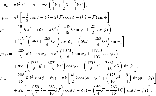 \begin{align} p_h &= \pi k^2 \mathcal{F} \,, \quad p_a = \pi k \left ( \frac {3}{4} k + \frac {1}{2} \mathcal{G} + \frac {3}{4} k \mathcal{F} \right)\!, \nonumber \\ p_{ha}&= \pi k \left [ - \frac {1}{2} \cos \phi - (\mathcal{G} + 2 k \mathcal{F}) \cos \phi + (k \mathcal{G} - \mathcal{F}) \sin \phi \right]\!, \nonumber \\ p_{hd1}&= - \frac {48}{5} \, R \, k^3 \sin \psi _1 + \pi k^2 \left ( -\frac {149}{16} k \sin \psi _1+ \frac {25}{2} \cos \psi _1 \right) \nonumber \\ &\quad + \frac {\pi k}{2} \left [ \left (59 \mathcal{G} + \frac {263}{4} k \mathcal{F} \right) \cos \psi _1+ \left ( 59 \mathcal{F} - \frac {263}{4} k \mathcal{G} \right) \sin \psi _1 \right]\!, \nonumber \\ p_{hd2}&= - \frac {208}{3} \, R \, k^3 \sin \psi _2 - \pi k^2 \left ( \frac {1073}{16} k \sin \psi _2+\frac {11720}{103} \cos \psi _2 \right) \nonumber \\ &\quad+ \pi k \left [ \left (\frac {1755}{8} \mathcal{G} + \frac {3831}{16} k \mathcal{F} \right) \cos \psi _2+ \left ( \frac {1755}{8} \mathcal{F} - \frac {3831}{16} k \mathcal{G} \right) \sin \psi _2 \right]\!, \nonumber \\ p_{ad1}&= - \frac {208}{15} \, R \, k^3 \sin (\phi -\psi _1) - \pi k \left [ \frac {41}{2} k \cos (\phi -\psi _1) + \left ( \frac {175}{16} k^2 - \frac {9}{4} \right) \sin (\phi - \psi _1) \right] \nonumber \\ &\quad+ \pi k \left [ - \left ( \frac {59}{4} \mathcal{G} + \frac {263}{16} k \mathcal{F} \right) \cos (\phi -\psi _1)+ \left ( \frac {59}{4} \mathcal{F} -\frac {263}{16} k \mathcal{G} \right) \sin (\phi -\psi _1) \right]\!, \end{align}
and
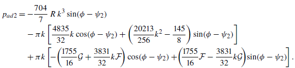 \begin{align} p_{ad2} &= - \frac {704}{7} \, R \, k^3 \sin (\phi -\psi _2)\nonumber \\ &\quad - \pi k \left [ \frac {4835}{32} k \cos (\phi -\psi _2) + \left ( \frac {20213}{256} k^2 -\frac {145}{8} \right) \sin (\phi - \psi _2) \right] \nonumber \\ &\quad + \pi k \left [ \!- \!\left (\!\frac {1755}{16} \mathcal{G} + \frac {3831}{32} k \mathcal{F} \!\right) \cos (\phi -\psi _2)+ \!\left (\! \frac {1755}{16} \mathcal{F} -\frac {3831}{32} k \mathcal{G} \!\right)\! \sin (\phi -\psi _2)\! \right] . \end{align}


 Open access