


1. Introduction
Shock–isotropic turbulence interactions (SITIs) are canonical flows where isotropic turbulence (and more generally also sound and/or entropy variations) passes through nominally planar normal shocks. These interactions emit vortical, acoustic and entropic fluctuations in the post-shock region, often at strengths significantly amplified relative to the incident fluctuations. Despite being simplified to a tractable scope, SITIs offer insights into the physics of the shock interaction of freestream disturbances, which is one component of the more general shock–turbulence interaction problem.
SITI flows are characterized typically by the upstream mean Mach number  $M$, the Mach number $M_t$ of the upstream turbulent velocity fluctuations, and the Taylor-scale Reynolds number $Re_\lambda$. In addition, the degree of compressibility of the upstream flow must be specified when it is not negligible; a convenient measure is the fraction $\chi$ of dilatational turbulent kinetic energy (TKE) to total TKE. Exact definitions of these parameters are given in § 3.
A fairly extensive collection of SITI direct numerical simulation (DNS) studies has been reported in the literature, beginning with the pioneering three-dimensional DNS by Lee, Lele & Moin (Reference Lee, Lele and Moin1993), who resolved the shock wave structure and studied the effects of  $M$ and $M_t$ in the regime of quasi-incompressible turbulence interacting with weak shocks. Hannappel & Friedrich (Reference Hannappel and Friedrich1995) reported shock-capturing SITI DNS at Mach 2 with varying $\chi$ and a relatively low $Re_\lambda$. They found that a greater $\chi$ led to greater amplification of transverse vorticity but lesser amplification of TKE and thermodynamic fluctuations. Lee, Lele & Moin (Reference Lee, Lele and Moin1997) used shock-capturing DNS to probe the effects of greater shock strength. Mahesh et al. (Reference Mahesh, Lee, Lele and Moin1995) used shock-capturing DNS to study incident fields of sound in the same SITI geometry, and Mahesh, Lele & Moin (Reference Mahesh, Lele and Moin1997) studied incident turbulent fields with correlated entropy fluctuations. Jamme et al. (Reference Jamme, Cazalbou, Torres and Chassaing2002) used shock-resolved DNS primarily to study the influence of the type or family of incident fluctuations (i.e. vortical, acoustic, entropic). They reported budgets to confirm that it is the baroclinic terms that lead to increased production of transverse vorticity fluctuations in cases where the correlation between upstream velocity and entropy fluctuations satisfies the Strong Reynolds Analogy, as had been suggested by Mahesh et al. (Reference Mahesh, Lele and Moin1997).
Larsson & Lele (Reference Larsson and Lele2009) explored a range of  $M$ and $M_t$ at higher $Re_\lambda$ than accessible previously, and reported many findings, including the fact that a decrease in the Kolmogorov scale across the interaction region persists downstream, and that therefore the post-shock region requires greater grid resolution than understood previously. They also studied profiles conditioned on the instantaneous shock strength, finding that locally stronger shocks resulted in temporary over-compression and that, depending on the flow parameters, locally weaker shocks corresponded to either discontinuous under-compression indicative of a wrinkled but intact shock front, or a smooth structure indicative of a broken shock front. Larsson, Bermejo-Moreno & Lele (Reference Larsson, Bermejo-Moreno and Lele2013) expanded on the dataset of Larsson & Lele (Reference Larsson and Lele2009) in order to further study the effects of $M_t$ and $Re_\lambda$. Among their findings was a criterion (discovered independently by Donzis Reference Donzis2012b) for predicting whether a set of parameters will fall into the wrinkled or broken shock regime.
Ryu & Livescu (Reference Ryu and Livescu2014) carried out shock-resolved SITI DNS to show convergence to linear interaction analysis (LIA) predictions in the limit of weak turbulence. They also introduced a method for using the equations of LIA (rather than DNS of the shock interaction) to process the upstream fluctuations in order to create an artificial post-shock field that mimics SITI at Reynolds numbers impractical for DNS. Sethuraman, Sinha & Larsson (Reference Sethuraman, Sinha and Larsson2018) focused on the thermodynamic fluctuations, demonstrating good agreement between DNS and LIA theory, and using budgets of transport equations to identify the mechanisms responsible for the streamwise evolution. Chen & Donzis (Reference Chen and Donzis2019) used shock-resolved SITI DNS with high  $M_t$ to study the effects of strong incident turbulence, especially the alteration of post-shock mean variables away from their classical Rankine–Hugoniot values. They also used their new data to revisit the studies of turbulence amplification and shock dilatation fluctuations of Donzis (Reference Donzis2012a,Reference Donzisb), respectively. Rather than focusing on the levels of various fluctuations through the interaction, Tanaka et al. (Reference Tanaka, Watanabe, Nagata, Sasoh, Sakai and Hayase2018) and Tanaka, Watanabe & Nagata (Reference Tanaka, Watanabe and Nagata2020) used SITI DNS to study the local connections between pre-shock velocity fluctuations, shock deformations, and post-shock pressure fluctuations. They considered both transient and quasi-steady cases. Among their findings were a Gaussian p.d.f. for the fluctuations in shock displacement, and positive correlations between shock normal velocity (towards the shock), shock strength and shock deformation towards the high pressure side. They also confirmed that the integral scale of the pre-shock turbulence is responsible for the spatial distribution of the fluctuations in shock strength and deformation.
The forgoing studies focused on SITI with a single fluid, but DNS in the SITI geometry has also been used to study more complex phenomena. Tian et al. (Reference Tian, Jaberi, Li and Livescu2017) studied the effects of density variations on SITI in one- and two-fluid cases, finding that the presence of density fluctuations intensified many effects of the canonical interaction. Notably, they also showed that shock-capturing SITI simulations converge to LIA in the limit of weak fluctuations. Tian, Jaberi & Livescu (Reference Tian, Jaberi and Livescu2019) used additional DNS results with velocity gradient tensor analysis to study how variable pre-shock density affects the post-shock turbulent structure and flow topology. Boukharfane, Bouali & Mura (Reference Boukharfane, Bouali and Mura2018) introduced passive scalar fields into SITI DNS problems to study the enhancement of scalar dissipation rate due to the shock interaction. Finally, Gao, Bermejo-Moreno & Larsson (Reference Gao, Bermejo-Moreno and Larsson2020) extended the study of SITI with passive scalars to a wider parameter space that included both the wrinkled and broken shock regimes.
DNS of turbulence interactions with reacting shocks has also been carried out to study the closely related problem of detonation–turbulence interactions. Examples include Massa, Chauhan & Lu (Reference Massa, Chauhan and Lu2011) and Huete et al. (Reference Huete, Jin, Martínez-Ruiz and Luo2017), who used DNS to study interactions with both stable and unstable reacting shocks. In the case of unstable shocks, the chemical reactions were shown to be capable of producing great increases in post-shock turbulence levels.
Confining attention to canonical non-reacting, single-fluid SITI DNS studies at moderate to high Reynolds number with primarily vortical incident fluctuations, the relevant cases from Lee et al. (Reference Lee, Lele and Moin1993, Reference Lee, Lele and Moin1997), Mahesh et al. (Reference Mahesh, Lele and Moin1997), Larsson & Lele (Reference Larsson and Lele2009), Larsson et al. (Reference Larsson, Bermejo-Moreno and Lele2013), Ryu & Livescu (Reference Ryu and Livescu2014), Tian et al. (Reference Tian, Jaberi, Li and Livescu2017, Reference Tian, Jaberi and Livescu2019), Huete et al. (Reference Huete, Jin, Martínez-Ruiz and Luo2017), Sethuraman et al. (Reference Sethuraman, Sinha and Larsson2018), Boukharfane et al. (Reference Boukharfane, Bouali and Mura2018), Tanaka et al. (Reference Tanaka, Watanabe, Nagata, Sasoh, Sakai and Hayase2018, Reference Tanaka, Watanabe and Nagata2020), Chen & Donzis (Reference Chen and Donzis2019) and Gao et al. (Reference Gao, Bermejo-Moreno and Larsson2020) cover a wide range of Mach numbers  $M$ and turbulence intensities ${\sim }M_t/M$. The highest turbulence intensities in these studies have been achieved through a combination of modest turbulence Mach numbers and low supersonic mean Mach numbers. Grube & Martín (Reference Grube and Martín2023) add data points from the regime featuring a high turbulence Mach number (or, equivalently, high root-mean-square (r.m.s.) Mach number fluctuation) combined with high mean Mach number. See figure 1. This previously unexplored regime is significant because linear theory (Ribner Reference Ribner1954a,Reference Ribnerb; Moore Reference Moore1954; Kerrebrock Reference Kerrebrock1956; Mahesh et al. Reference Mahesh, Lee, Lele and Moin1995) predicts significantly different amplification factors for high versus low supersonic mean Mach numbers, and also because high turbulence Mach numbers imply the appearance of dilatational motions in the incident turbulence. These dilatational motions are amplified according to a separate set of transfer functions with behaviour very different from that of the transfer functions for solenoidal turbulence.

Figure 1. Mach number and disturbance intensity parameter space for previous and current moderate- to high- $Re$ SITI DNS studies: Lee et al. (Reference Lee, Lele and Moin1993) ( $\triangleleft$, black) and Lee et al. (Reference Lee, Lele and Moin1997) ( $\triangleright$, black), Mahesh et al. (Reference Mahesh, Lele and Moin1997) ( $\triangle$, black), Larsson & Lele (Reference Larsson and Lele2009) and Larsson et al. (Reference Larsson, Bermejo-Moreno and Lele2013) ( $\square$, green), Huete et al. (Reference Huete, Jin, Martínez-Ruiz and Luo2017) ( $\times$, red), Tian et al. (Reference Tian, Jaberi, Li and Livescu2017, Reference Tian, Jaberi and Livescu2019) ( $\circ$, purple), Boukharfane et al. (Reference Boukharfane, Bouali and Mura2018) ( $\bigtriangledown$, pink), Sethuraman et al. (Reference Sethuraman, Sinha and Larsson2018) ( $\otimes$, green), Tanaka et al. (Reference Tanaka, Watanabe, Nagata, Sasoh, Sakai and Hayase2018, Reference Tanaka, Watanabe and Nagata2020) (
![]() , blue), Chen & Donzis (Reference Chen and Donzis2019) (
, blue), Chen & Donzis (Reference Chen and Donzis2019) ( $\diamond$, blue), Gao et al. (Reference Gao, Bermejo-Moreno and Larsson2020) ( $+$, green), present work/Grube & Martín (Reference Grube and Martín2023) ( $\bullet$, red). In addition, Ryu & Livescu (Reference Ryu and Livescu2014) provided fairly dense, systematic coverage of the boxed area of the parameter space. The approximate boundary between the broken and wrinkled shock regimes is shown as a dashed line. The regime criterion is based on Larsson et al. (Reference Larsson, Bermejo-Moreno and Lele2013) and Donzis (Reference Donzis2012b), with $M_t$ converted to $M'_{rms}$ using $M'_{rms}\approx M_t/\sqrt {3}$ for the primarily solenoidal turbulence of their dataset. Figure from Grube & Martín (Reference Grube and Martín2023).
The characterization of the inflow is complicated by the fact that the incident pressure field contains two types of fluctuations. There are non-propagating pressure fluctuations associated with vorticity fields. We will refer to these captive pressure fluctuations as pseudo-sound. The lower pressure region found at the centre of an isolated vortex is an example of pseudo-sound. In contrast to non-propagating pseudo-sound, propagating acoustic disturbances can also be generated through nonlinear interactions between vortical modes (Chu & Kovasznay Reference Chu and Kovasznay1957) or through exothermic reactions (Martin & Candler Reference Martin and Candler1998) or other mechanisms. Pseudo-sound pressure fluctuations have no velocity fluctuations of their own; they arise in association with vortical velocity fluctuations. In contrast, acoustic disturbances possess dilatational velocity fluctuations in addition to isentropic thermodynamic fluctuations.
From pressure fluctuation data alone, it is impossible to distinguish between pseudo-sound and acoustic contributions. However, by assuming that all of the observed pressure fluctuations arise from acoustic waves, we can compute an upper bound on the fraction  $\chi$ of the TKE that could be attributable to dilatational modes. In an acoustic wave, the dilatational velocity fluctuation is related to the pressure fluctuation by $p'_{rms}=\rho c \left | \boldsymbol {u}^{\prime \prime \, dil.} \right |_{rms}$ where ${p'_{rms}}$ is the r.m.s. pressure fluctuation, $\rho$ is the density, $c$ is the speed of sound, and $\left | \boldsymbol {u}^{\prime \prime \,dil.} \right |_{rms}$ is the r.m.s. magnitude of the dilatational Favre velocity fluctuation. If the pressure fluctuation field were due entirely to acoustic waves, then the ratio $\chi$ of dilatational TKE to total TKE would be $\chi = ( {p'_{rms}}/{\gamma p M_t})^2$. Larsson et al. (Reference Larsson, Bermejo-Moreno and Lele2013) report the $p'$ values for their wide range of cases through the relation ${p'_{rms}}/{\gamma p M_t^2}=0.39 \pm 0.02$. However, this relation depends on the details of how the inflow turbulence is generated; the two nominally solenoidal cases of Jamme et al. (Reference Jamme, Cazalbou, Torres and Chassaing2002) lead to values 0.50 and 0.53, which fall outside the range observed by Larsson & Lele (Reference Larsson and Lele2009). Nevertheless, the pressure fluctuation level, once known, yields an estimate on the upper bound for the dilatational TKE fraction $\chi$. In the case of Larsson & Lele (Reference Larsson and Lele2009), this upper bound becomes $\chi < 0.39^2M_t^2 = 0.15 M_t^2$. Thus their highest $M_t$ value of 0.38 implies an upper bound $\chi < 2.2\,\%$. Given the similarity in methods between the two studies, this upper bound is likely applicable to Larsson et al. (Reference Larsson, Bermejo-Moreno and Lele2013) as well. Similarly, the computed upper bound for the solenoidal cases of Jamme et al. (Reference Jamme, Cazalbou, Torres and Chassaing2002) is $\chi < 1.5\,\%$.
The parameters of Chen & Donzis (Reference Chen and Donzis2019) include a maximum  $M_t$ value of 0.54. They do not report $\chi$ or pressure fluctuation levels, but if we assume a value ${p'_{rms}}/{\gamma p M_t^2}=0.53$ (as in the most extreme case of Jamme et al. (Reference Jamme, Cazalbou, Torres and Chassaing2002) in order to obtain a conservative estimate), then $M_t=0.54$ gives an upper bound $\chi \lessapprox 8.2\,\%$. We stress that this is only a bound, and there is no reason to expect that the majority of the pressure fluctuations are truly from acoustic waves as opposed to pseudo-sound.
In flows where the pressure fluctuations arise mainly from pseudo-sound and/or from acoustic waves generated by quadratic interactions of vortical modes, the true values of  $\chi$ may remain modest. Some researchers have studied more highly dilatational inflows by producing the dilatational modes through initial conditions or through forcing. Mahesh et al. (Reference Mahesh, Lee, Lele and Moin1995) studied a purely acoustic inflow field, and others have considered vortical turbulence accompanied by an unusually high level of dilatation. In addition to their vortical cases mentioned above, Jamme et al. (Reference Jamme, Cazalbou, Torres and Chassaing2002) also considered cases with primarily dilatational velocity fluctuations that featured upper bounds on $\chi$ as high as $71\,\%$, and Hannappel & Friedrich (Reference Hannappel and Friedrich1995) featured a case with true value (not upper bound) $\chi =0.5$. However, the dilatational cases of both Jamme et al. (Reference Jamme, Cazalbou, Torres and Chassaing2002) and Hannappel & Friedrich (Reference Hannappel and Friedrich1995) were limited to $Re_\lambda =5$, and therefore may exhibit low- $Re$ effects.
Grube & Martín (Reference Grube and Martín2023) report the DNS of highly compressible SITI cases with  $M_t$ up to 0.69, $Re_\lambda$ up to 48, and true values up to 15 % of the TKE in dilatational modes. Thus their data explore more highly dilatational turbulence than has been studied aside from the $Re_\lambda =5$ cases of Jamme et al. (Reference Jamme, Cazalbou, Torres and Chassaing2002) and Hannappel & Friedrich (Reference Hannappel and Friedrich1995). This paper discusses the relationships between this dataset and studies in the literature regarding Reynolds stress amplification (Donzis Reference Donzis2012a) and shock structure modification (Donzis Reference Donzis2012b), as well as the threshold for transition between the wrinkled and broken shock regimes (Donzis Reference Donzis2012b; Larsson et al. Reference Larsson, Bermejo-Moreno and Lele2013). It is organized as follows. Section 2 summarizes the governing equations and the numerical methods used to solve them. Section 3 lists the flow parameters of the SITI cases under consideration. Section 4 examines the cause of the unusually high amplification of streamwise Reynolds stress observed in these highly compressible SITI cases as compared to other cases in the literature. Section 5 compares the modifications to the shock structure caused by the highly compressible incident turbulence against those proposed by Donzis (Reference Donzis2012b), and § 6 proposes a re-parametrization of the shock structure data that accounts for acoustic and entropy fluctuations in order to better collapse the highly compressible SITI data with the more solenoidal inflow cases from the literature. Finally, § 7 summarizes the results.
2. Governing equations and numerical method
The flow is governed by the three-dimensional conservation equations for mass, momentum and energy:
 \begin{gather} \frac{\partial\rho}{\partial t}+\frac{\partial}{\partial x_j}(\rho u_j)=0, \end{gather}
 \begin{gather} \frac{\partial (\rho u_i)}{\partial t}+\frac{\partial}{\partial x_j}(\rho u_i u_j+p\,\delta_{ij}-\sigma_{ij})=0, \end{gather}
 \begin{gather} \frac{\partial E}{\partial t}+\frac{\partial}{\partial x_j}\left[\left(E+p\right)u_j-\sigma_{ij}u_i+q_j\right]=0, \end{gather}
 in which  $\rho$ is the fluid density, $u_i$ is the velocity component in the $x_i$ direction, $p$ is the thermodynamic pressure, and $E=\rho e + \tfrac 12\rho {\boldsymbol u} \boldsymbol{\cdot }{\boldsymbol u}$ is the total energy (internal plus kinetic) of the fluid per unit volume. The air is treated as a perfect gas; therefore the equation of state is $p=\rho RT$, where $R=287.1\,{\rm J}\,{\rm kg}^{-1}\,{\rm K}^{-1}$. The speed of sound is $c=\sqrt {\gamma R T}$, where $\gamma =1.4$, and the specific internal energy is $e=c_v T$, where $c_v=2.5R$. The viscous stress tensor $\sigma _{ij}$ is assumed to obey a linear stress–strain relationship:
 \begin{equation} \sigma_{ij}=\mu\left[\left(\frac{\partial u_i}{\partial x_j}+\frac{\partial u_j}{\partial x_i}\right)-\frac{2}{3}\,\frac{\partial u_k}{\partial x_k}\,\delta_{ij}\right]. \end{equation}
The viscosity  $\mu$ is assumed to depend only on temperature $T$ through a power law (White Reference White1991) of the form
 \begin{equation} \mu=\mu_0\left({T}/{T_0}\right)^n, \end{equation}
where  $\mu _0$ and $T_0$ are reference values that depend on the particular gas mixture. For air, we use $\mu _0=1.789\times {10}^{-5}\,\mathrm {Pa}\,{\mathrm {s}}$, $T_0=288.2\,\mathrm {K}$ and $n=0.76$. The heat flux $q_i$ is computed through Fourier's law of heat conduction,
 \begin{equation} q_i={-}\kappa\,{\frac{\partial }{\partial x_i}}T, \end{equation}
in which  $\kappa$ is the thermal conductivity. The thermal conductivity is related to the viscosity by the Prandtl number $Pr\equiv {c_p \,\mu }/{\kappa }\approx 0.7368$.
The mean flow is directed in the positive  $x_1$ direction, and the mean shock location is used as the origin for the $x_1$ coordinate.
We define  $\bar {\eta }$ as the average value of a generic quantity $\eta$ aggregated over time and all homogeneous spatial directions (two transverse directions in SITI flows, and three directions in auxiliary isotropic turbulence computations), $\eta ^\prime \equiv \eta - \bar {\eta }$ as the associated local fluctuation, and $\tilde {\eta }\equiv \overline {\rho \eta }/\bar {\rho }$ and $\eta ^{\prime \prime }\equiv \eta -\tilde {\eta }$ as the corresponding density-weighted (Favre) average and fluctuation, respectively.
Grube & Martín (Reference Grube and Martín2023) solved the governing equations using a finite-difference code with a fourth-order-accurate version of the linearly and nonlinearly optimized WENO-SYMBO scheme (Weirs & Candler Reference Weirs and Candler1997; Martín et al. Reference Martín, Taylor, Wu and Weirs2006; Taylor & Martín Reference Taylor and Martín2007) for the convective terms, and a fourth-order-accurate standard central-difference scheme for the viscous terms. The solution was advanced in time using the third-order-accurate low-storage Runge–Kutta method of Williamson (Reference Williamson1980) with Courant–Friedrichs–Lewy (CFL) number  $0.5$.
Turbulence data for the supersonic inflow boundary were provided by an auxiliary forced isotropic turbulence simulation (Grube & Martín Reference Grube and Martín2023). Relatively high and low values of  $\chi$ could be achieved by choosing to force all turbulent modes or only solenoidal ones. A sponge zone was used to smoothly damp post-shock fluctuations and prevent acoustic reflections from the subsonic outflow, and periodic boundary conditions were applied in the transverse directions.
The naming scheme for the DNS cases of Grube & Martín (Reference Grube and Martín2023) is explained in § 3; each case name consists of a letter and a number. In all cases, the grid was 2.5 times finer in the streamwise direction than in the homogeneous directions. Cases in the N-series used 600 grid points in the homogeneous directions, with 1500 interior points in the streamwise direction, plus an additional 375 streamwise points in the sponge zone. Case L1 was at a slightly lower Reynolds number and therefore used 450 points in the homogeneous directions, 1125 in the streamwise direction and 282 in the sponge zone. The C-series cases were at still lower Reynolds numbers and used 300 points in the homogeneous directions, 750 in the streamwise direction and 75 in the sponge zone.
Parameters of the computational grids are reported in table 1:  $N_1$, $N_2$ and $N_3$ are the numbers of grid points within the useful computational domain in the streamwise and two homogeneous directions, respectively; $N_{sp}$ is the number of additional streamwise points used in the sponge zone at the outflow. There are $\eta _{u\vert d}/\Delta {x_1}$ streamwise grid points per Kolmogorov scale $\eta$ on the upstream and downstream sides of the shock, respectively. The least well resolved case was the case L1, which was computed for comparison with Larsson et al. (Reference Larsson, Bermejo-Moreno and Lele2013) as a check for errors in methodology. L1 featured approximately 0.9 streamwise points per Kolmogorov scale on the post-shock side, which is the most demanding region to resolve. The C- and N-series cases were of primary scientific interest, and they featured between 1.2 and 2.2 streamwise points per $\eta _d$.
Table 1. Grid parameters.

3. Flow parameters
Four non-dimensional parameters are used to characterize the state of the incident turbulent flow: the Taylor microscale Reynolds number  ${Re}_\lambda ={\bar {\rho } u^{\prime \prime }_{1,{rms}}\,\lambda }/{\bar {\mu }}$, the turbulent Mach number $M_t={q}/{\bar {c}}$, the mean Mach number $M={\tilde {u}}/{\bar {c}}$, and the ratio $\chi$ of dilatational to total TKE. Here, $q\equiv \sqrt {R_{kk}}$ is the r.m.s. magnitude of the velocity fluctuation, and $R_{ij}\equiv \widetilde {u''_iu''_j}$ is the Reynolds stress tensor. Computing $\chi$ begins with the Helmholtz decomposition of the velocity fluctuation field into solenoidal and dilatational parts, $\boldsymbol {u}''=\boldsymbol {u}''^{\,sol.}+\boldsymbol {u}''^{\,dil.}$, such that $\boldsymbol {\nabla } \boldsymbol{\cdot }\boldsymbol {u}''^{\,sol.}=0$ and $\boldsymbol {\nabla }\times \boldsymbol {u}''^{\,dil.}=0$. Then $\chi \equiv \int \vert \boldsymbol {u}''^{\,dil.} \vert ^2 \,{\rm d}\boldsymbol {x}/\int \vert \boldsymbol {u}'' \vert ^2 \,{\rm d}\boldsymbol {x}$, where the integration is taken over a statistically homogeneous region. We follow previous SITI works (Lee et al. Reference Lee, Lele and Moin1993, Reference Lee, Lele and Moin1997; Mahesh et al. Reference Mahesh, Lele and Moin1997; Larsson & Lele Reference Larsson and Lele2009; Larsson et al. Reference Larsson, Bermejo-Moreno and Lele2013) in using a Taylor microscale defined by Tennekes & Lumley (Reference Tennekes and Lumley1972):
 \begin{equation} \lambda =u^{\prime\prime}_{\alpha,{rms}}/\sqrt{\overline{({\partial u_\alpha}/{\partial x_\alpha})^2}} \quad\text{(with no summation over Greek indices)}, \end{equation}
where  $u^{\prime\prime}_{\alpha,{rms}}$ is the r.m.s. Favre fluctuation of $\alpha$ direction velocity. (In homogeneous turbulence, the choice of $\alpha$ is immaterial.) Under the definitions given by Pope (Reference Pope2000), this Taylor microscale is a factor of $\sqrt {2}$ less than the longitudinal Taylor microscale $\lambda _f$ and in incompressible isotropic turbulence is equivalent to the transverse microscale $\lambda _g$.
As mentioned above, the SITI DNS cases of Grube & Martín (Reference Grube and Martín2023) are each designated by a letter–number combination (e.g. C1, N2). All but one of the DNS cases belong to one of two series, the C-series and the N-series. The C-series cases C1, C2 and C3 included turbulence Mach numbers that were unprecedented in SITI studies; questions raised by the case C1–C3 results motivated the rest of the DNS cases. In addition to higher  $M_t$ values, cases C1–C3 also featured an unusually high compressibility ratio $\chi =11\,\%$, and somewhat lower Reynolds numbers ( $Re_\lambda =18\unicode{x2013}25$) than some of the other cases available in the literature, such as Larsson & Lele (Reference Larsson and Lele2009) and Larsson et al. (Reference Larsson, Bermejo-Moreno and Lele2013).
Because the C-series cases simultaneously featured lower  $Re_\lambda$, higher $\chi$, and higher $M_t$ than previous studies, it was difficult to determine which of these differences might be responsible for the observed results. This difficulty motivated additional DNS cases undertaken in order to better isolate the effects of $Re_\lambda$ and $\chi$. The new cases included the N-series, with generally lower $\chi$ and higher $Re_\lambda$ than C1–C3, as well as a new case C4 that differs from C1 only in having lower $\chi$. Finally, in order to help rule out errors in methodology, case L1 was designed to match approximately a case already studied by Larsson et al. (Reference Larsson, Bermejo-Moreno and Lele2013).
The flow parameters for the DNS cases are listed in table 2. All parameters except for  $\chi$ are extrapolated to the mean shock location. Decomposing the pre-shock flow into solenoidal and dilatational components was hampered by the spatial inhomogeneity of the flow (i.e. by the shock wave and by the gradual decay of certain properties between the inflow and the shock location). Therefore the fraction $\chi$ of TKE in the dilatational modes is computed using the Fourier transform of the auxiliary forced isotropic turbulence field that supplies the inflow data.
Table 2. Upstream flow parameters extrapolated to the mean shock location.

Each entry in the table is accompanied by a comment explaining the significance of that particular case. There are ‘base’ cases (numbered 1) for the C- and N-series, and then the other cases differ from their respective base case mainly in the manner noted in the comment column. For example, case N2 is labelled  $M_t\uparrow$ because it can be compared against the base case N1 to determine the effect of increasing turbulence Mach number.
The SITI inflow disturbances are primarily a mixture of solenoidal (vortical) turbulence and dilatational (acoustic) modes. Entropy fluctuations  $s'/c_p$ are approximately an order of magnitude smaller.
4. Streamwise Reynolds stress amplification factors
The parameter choices for the N-series DNS cases as well as cases C4 and L1 were motivated partially by the need for data points to investigate the unusually high streamwise Reynolds stress amplification levels observed in cases C1 and C3. Donzis (Reference Donzis2012a) considered DNS SITI studies from the literature and compiled values of the amplification factor  $G_{11} \equiv R_{{11}_{u,min}}/R_{{11}_{d, max}}$, where subscripts $u,min$ and $d,max$ denote upstream and downstream minimum and maximum values, respectively. Donzis (Reference Donzis2012a) proposed a universal relation between $G_{11}$ and the dimensionless parameter $K\equiv M_t/(\sqrt {Re_\lambda } (M-1))$, which is proportional to the ratio of the shock thickness to the Kolmogorov scale. Ryu & Livescu (Reference Ryu and Livescu2014) pointed out that the proposed parametrization by $K$ alone conflicted with the Mach number dependence of $G_{11}$ in the inviscid, weak turbulence limit, and the original parametrization has since been superseded by the more sophisticated analysis of Chen & Donzis (Reference Chen and Donzis2019) which takes the Mach number into account. Nevertheless, the original Mach-number-insensitive parametrization remains helpful as a means of separating visually the data points in order to place the present results in the context of previous works. However, as discussed in Chen & Donzis (Reference Chen and Donzis2019), the data points should not be expected to collapse completely onto this single curve.
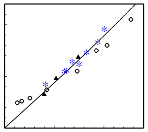
Table 3 lists the values of  $G_{11}$ computed from the current DNS cases, and figure 2 plots them on top of Donzis's compiled data. The greatest value of $G_{11}$ from the literature is approximately 1.7, which was observed in a case from Larsson & Lele (Reference Larsson and Lele2009). The amplification factors of cases C1 and C3 (1.97 and 2.22, respectively) are considerably higher than 1.7. In order to help rule out errors in methodology, the parameters of case L1 were chosen to match approximately a case of Larsson & Lele (Reference Larsson and Lele2009). The amplification factor computed for case L1 is 1.73, which differs by approximately 3.5 % from the amplification factor of 1.67 observed in the similar case ( $M=3.5$, $M_t=0.22$, $Re_\lambda \approx 40$) of Larsson & Lele (Reference Larsson and Lele2009). This level of agreement indicates that differences in methodology are unlikely to account for the majority of the higher amplification factors observed in cases C1 and C3 compared to previous cases in the literature.

Figure 2. Reynolds stress  $R_{11}$ amplification factor $G_{11}$ versus $K\equiv {M_t} / {Re_\lambda ^{1/2} (M-1)}$: current DNS results ( $\ast$, blue), Lee et al. (Reference Lee, Lele and Moin1993) ( $\blacktriangleright$), Hannappel & Friedrich (Reference Hannappel and Friedrich1995) ( $\Diamond$), Barre, Alem & Bonnet (Reference Barre, Alem and Bonnet1996) ( $\blacktriangleleft$), Lee et al. (Reference Lee, Lele and Moin1997) ( $\square$), Mahesh et al. (Reference Mahesh, Lele and Moin1997) ( $\triangledown$), Jamme et al. (Reference Jamme, Cazalbou, Torres and Chassaing2002) ( $\bullet$), Larsson & Lele (Reference Larsson and Lele2009) ( $\vartriangle$), Boukharfane et al. (Reference Boukharfane, Bouali and Mura2018) ( $\blacktriangle$). The solid line is the original proposed fit of Donzis (Reference Donzis2012a). Note that the proposed fit has been superseded by the more sophisticated analysis of (Chen & Donzis Reference Chen and Donzis2019). It is used here for its simplicity (i.e. lack of Mach number dependence) and for a means of separating the data points visually. Data points should not be expected to collapse completely. Adapted from Donzis (Reference Donzis2012a).
Table 3. Amplification factors  $G_{11}$ for streamwise Reynolds stress $R_{11}$. In order to facilitate comparison with the data compiled by Donzis (Reference Donzis2012a), the values of $R_{11}$ used in computing $G_{11}$ are the pre-shock minimum and the post-shock maximum.

Pairwise comparisons of the C- and N-series DNS cases reveal the effects of varying the flow parameters. Comparing C2 ( $M_t\uparrow$) to C3 ( $M_t \uparrow M\uparrow$), and N1 (base) to N3 ( $M\uparrow$), we see that increasing $M$ tends to increase $G_{11}$. Comparing C4 ( $\chi \downarrow$) to C1 (base), and N1 (base) to N4 ( $\chi \uparrow$), we see that increasing $\chi$ tends to increase $G_{11}$. Comparing C1 (base) to C2 ( $M_t\uparrow$), and N1 (base) to N2 ( $M_t\uparrow$), we see that increasing $M_t$ tends to decrease $G_{11}$. Finally, the Reynolds numbers of the C-series ( $Re_\lambda = 18\unicode{x2013}27$) and N-series ( $Re_\lambda = 41\unicode{x2013}48$) cases bracket the value $Re_\lambda \approx 40$ for the cases in Larsson & Lele (Reference Larsson and Lele2009). Since cases from both the C- and N-series show elevated values of $G_{11}$ relative to the results of Larsson & Lele (Reference Larsson and Lele2009), it appears that the effect is not closely related to the Reynolds number.
We therefore hypothesize that the elevated amplification factors  $G_{11}$ arise from a combination of high $M$ and high $\chi$. LIA can be applied separately to the solenoidal and dilatational modes of incident turbulence. While the solenoidal part of the incident TKE (a fraction $1-\chi$) is amplified in the linear limit according to the familiar vortical or solenoidal transfer functions (Ribner Reference Ribner1954a,Reference Ribnerb), the dilatational part (a fraction $\chi$) is amplified according to a different set of transfer functions (Moore Reference Moore1954; Kerrebrock Reference Kerrebrock1956; Mahesh et al. Reference Mahesh, Lee, Lele and Moin1995). It is found that although the solenoidal transfer functions remain of order 1, their dilatational or acoustic counterparts grow as $M^2$ for high Mach numbers.
Figure 3 presents transfer functions  $\vert X_{a\rightarrow b}\vert ^2$ that relate incident streamwise velocity fluctuation levels $(u''_{1,u, rms}/\tilde {u}_{1,u})^2$ to emitted streamwise velocity fluctuation levels $(u''_{1,d, rms}/\tilde {u}_{1,u})^2$ as functions of upstream Mach number. The generic subscripts $a$ and $b$ can represent $p$ or $v$, which stand for the pressure (dilatational) and vortical (solenoidal) parts of the velocity fields. The dilatational field is further broken down into near-field and far-field values. Because Donzis (Reference Donzis2012a) defines the amplification factor $G_{11}$ in terms of the post-shock maximum value of $R_{11}$, which occurs relatively far from the shock in comparison to the spatial evolution of the acoustic field, the far-field acoustic values are of more interest than the near-field values in this context. Therefore, above approximately Mach 3, the post-shock velocity field due to the interaction of incident dilatational modes is dominated by its solenoidal part.

Figure 3. Linear amplification factors for dilatational velocity fluctuations.
Thus at high enough mean Mach number, the Reynolds stress amplification factor for incident dilatational modes greatly exceeds that for incident vortical modes. This is true for both the streamwise and transverse Reynolds stress transfer functions. It can be seen in Reynolds stress budgets such as those in Grube, Taylor & Martín (Reference Grube, Taylor and Martín2011) or Larsson et al. (Reference Larsson, Bermejo-Moreno and Lele2013) that nonlinear effects in the post-shock region redistribute TKE from  $R_{22}$ and $R_{33}$ to $R_{11}$. If similar nonlinear processes apply to the vortical field produced by the incident dilatational modes, then the actual contribution to $R_{11_{d, max}}$ due to the incident dilatational modes might be somewhat greater than indicated by $\vert X_{p\rightarrow v}\vert ^2$.
The greater transfer functions applicable to incident dilatational modes at high Mach numbers are consistent with the observation that the DNS cases with greatest  $G_{11}$ values feature both high $M$ and high $\chi$.
In order to assess quantitatively the plausibility of this explanation, let us estimate the contribution to  $G_{11}$ that is attributable solely to the solenoidal part of the incident field, and then compare this against the data from the literature. Because the incident dilatational modes and incident solenoidal modes are uncorrelated, the Reynolds stresses and TKE immediately behind the shock could be computed by simply adding the contributions from the vortical and dilatational incident modes (computed from $X_{v\rightarrow v}$ and $X_{p\rightarrow v}$). However, further downstream from the shock, where the streamwise maximum of $R_{11}$ is found, this way of combining the contributions becomes an approximation due to nonlinear effects (such as pressure–strain redistribution). There is also a viscous decay not captured by the inviscid LIA transfer functions. Nevertheless, in order to estimate the effects of the incident dilatational modes, let us assume that the dilatational and solenoidal transfer functions can be combined approximately in a weighted sum based on $\chi$. Since $X_{p\rightarrow v}$ dominates $X_{p\rightarrow p}^{ far}$, and since the evanescent waves corresponding to $X_{p\rightarrow p}^{near}$ will have largely decayed by the point of maximum $R_{11}$, we use $X_{p\rightarrow v}$ alone to estimate the contribution of the dilatational incident field to the post-shock Reynolds stress:
 \begin{equation} G_{11}\approx(1-\chi)G_{11}^{sol.}+\chi\vert X_{p\rightarrow v} \vert^2 . \end{equation}
Here,  $X_{p\rightarrow v}$ is computed from LIA, $G_{11}$ is the actual amplification factor computed from the DNS solution, and $G_{11}^{sol.}$ is an effective transfer function linking the solenoidal parts of the pre- and post-shock Reynolds stresses.
Since the works cited by Donzis (Reference Donzis2012a) all had relatively low  $\chi \vert X_{p\rightarrow v} \vert ^2$ (i.e. low $\chi$ and/or low $M$), it is appropriate to compare $G_{11}^{sol.}$ from the present work with the data compiled by Donzis. Solving (4.1) for the effective solenoidal amplification factor $G_{11}^{sol.}$, and plotting it against the compiled data (figure 4), we find that the solenoidal part of the amplification falls much closer to the range of the previous DNS works. In other words, after approximately removing the contribution from incident dilatational modes, the $R_{11}$ amplification factors of the present DNS lie near the data from previous works (which featured very little dilatational TKE in the inflow). This supports the hypothesis that the high $G_{11}$ values observed in the present DNS arise from significant levels of incident dilatational TKE combined with large values of $\vert X_{p\rightarrow v}\vert$ that result from high Mach numbers.

Figure 4. Effective solenoidal Reynolds stress  $R_{11}$ amplification factor $G^{sol.}_{11}$ versus $K=M_t/\sqrt {Re_\lambda }(M-1)$: current DNS results ( $\ast$, blue), Lee et al. (Reference Lee, Lele and Moin1993) ( $\blacktriangleright$), Hannappel & Friedrich (Reference Hannappel and Friedrich1995) ( $\Diamond$), Barre et al. (Reference Barre, Alem and Bonnet1996) ( $\blacktriangleleft$), Lee et al. (Reference Lee, Lele and Moin1997) ( $\square$), Mahesh et al. (Reference Mahesh, Lele and Moin1997) ( $\triangledown$), Jamme et al. (Reference Jamme, Cazalbou, Torres and Chassaing2002) ( $\bullet$), Larsson & Lele (Reference Larsson and Lele2009) ( $\vartriangle$), Boukharfane et al. (Reference Boukharfane, Bouali and Mura2018) ( $\blacktriangle$). The solid line is the proposed fit of Donzis (Reference Donzis2012a). Adapted from Donzis (Reference Donzis2012a).
However, we stress that parametrizing the amplification by the single parameter  $K$ still does not capture the Mach number dependence of the amplification factors and that (4.1) is only an approximate relation. In addition, the results are sensitive to $\chi$, the exact value of which is difficult to determine at $x_1=0$. The values of $\chi$ used in computing $G_{11}^{sol.}$ in figure 4 are based on the Fourier transforms of the auxiliary forced turbulence simulations, and these values may be inaccurate at the shock location due to differences in decay rates between vortical and dilatational turbulent motions as they travel from the inlet to the shock location. Furthermore, the eddies in the incident field have some level of pseudo-sound associated with them (i.e. pressure variations that convect along with the vorticity field rather than propagating as acoustic waves), and this pseudo-sound, although a second-order effect, may have transfer functions that scale as $M^2$, similar to the acoustic transfer functions. Thus perhaps the pseudo-sound, which is not accounted for in the present first-order analysis, may be related to the remaining gap between the $G_{11}^{sol.}$ values observed in cases N3 and N1, and those from previous works. The gap may also be related to the nonlinear terms that redistribute TKE from transverse to streamwise Reynolds stresses in the post-shock region; such effects would lead to a larger contribution by the dilatational modes than indicated by $\vert X_{p\rightarrow v}\vert ^2$ alone. Furthermore, we have chosen the far-field transfer function despite the fact that some of the evanescent near-field energy still persists at the location of the post-shock maximum.
5. Alteration of shock structure by incident fluctuations
To understand why cases C2 and N2 exhibit lower amplification than cases C1 and N1, respectively (i.e. why higher  $M_t$ leads to lower $G_{11}$), consider the ratio of the r.m.s. and mean values of the peak dilatation rate inside the shock. Define $\theta _{min}(x_2,x_3,t)\equiv \min _{x_1}\theta (x_1,x_2,x_3,t)$, where $\theta = \partial _{x_i}\!u_i$ is the dilatation rate. Then the ratio $\varTheta \equiv (\theta _{min})'_{rms}/\overline {\vert \theta _{min}\vert }$ characterizes the alteration of the shock structure due to the incident disturbances. An unperturbed shock corresponds to $\varTheta =0$, and increasing values of $\varTheta$ correspond to shocks with increasing variations in strength. Above some value of $\varTheta$, fluctuation events can completely cancel out the shock jump, leaving gaps in the shock surface. (This is the so-called broken shock regime, in which amplification falls precipitously.) As $\varTheta$ increases, such events become more common, and a greater fraction of the shock surface is replaced by areas of smooth compression. As pointed out by Larsson & Lele (Reference Larsson and Lele2009), computed values of $\varTheta$ continue to characterize the shock structure even in shock-capturing simulations where the dilatation computed within the shock is influenced by the grid spacing. Donzis (Reference Donzis2012b) shows that for the compilation of previous DNS results, $\varTheta$ is approximately a universal function of $M_t/(M-1)$, therefore $M_t/(M-1)$ serves as a measure of how broken or intact a shock is. Donzis (Reference Donzis2012b) and Larsson et al. (Reference Larsson, Bermejo-Moreno and Lele2013) arrive independently at the value $M_t/(M-1)\approx 0.6$ as the threshold between the wrinkled and broken shock regimes.
The normalized dilatation rate values from the present DNS are overlaid on the data compiled by Donzis (Reference Donzis2012b) in figure 5. The new data follow roughly Donzis's best-fit curve. Cases C2 and N2 have the highest  $\varTheta$ values of the present cases (0.19 and 0.17, respectively). Of the DNS cases studied by Larsson et al. (Reference Larsson, Bermejo-Moreno and Lele2013), the one with the highest value of $\varTheta$ that is judged by them to fall within the wrinkled shock regime is $\varTheta =0.21$, around 10 % greater than for case C2. Thus the range of present DNS cases is nearing the upper limit of $\varTheta$ for the wrinkled shock regime. The proximity of cases C2 and N2 to the broken shock regime where amplification falls off may explain why, in comparisons of C1 to C2 and N1 to N2, a higher $M_t$ appears to give lower $G_{11}$.

Figure 5. Normalized r.m.s. peak shock dilatation  $\varTheta$ as a function of $M_t/(M-1)$: current DNS results ( $\ast$, blue), Jamme et al. (Reference Jamme, Cazalbou, Torres and Chassaing2002) ( $\bullet$), Larsson & Lele (Reference Larsson and Lele2009) ( $\circ$ wrinkled, $\star$ transitional, $\square$ broken), Boukharfane et al. (Reference Boukharfane, Bouali and Mura2018) ( $\blacktriangle$). The solid line is the proposed curve of Donzis (Reference Donzis2012a). Adapted from Donzis (Reference Donzis2012a).
6. A generalized parametrization of the shock structure
Since the appearance of locally subsonic regions upstream of the shock signals the transition from the wrinkled to broken shock regimes, the difference between the local instantaneous Mach number  $\mathscr {M}$ and unity is of fundamental importance in parametrizing the modification of the shock structure. A measure of the velocity fluctuations can be obtained from $M_t$, and a measure of how large a velocity fluctuation is needed on average in order to reduce the flow to a locally subsonic value is provided by $M-1$. Therefore, parametrizing the shock structure (i.e. $\varTheta$) by the ratio $M_t/(M-1)$ as done by Donzis (Reference Donzis2012b) and Larsson et al. (Reference Larsson, Bermejo-Moreno and Lele2013) makes sense for incident solenoidal turbulence where the Mach number fluctuation arises solely from velocity fluctuations.
However, in flows with compressible isotropic turbulence incident on the shock, this parameter gives only part of the necessary information. The velocity field in this more general case can be decomposed into vortical (solenoidal) and acoustic (dilatational) parts. The vortical and acoustic parts give different contributions to the local Mach number fluctuation. Whereas the vortical part contributes only velocity fluctuations, the acoustic part is also associated with isentropic thermodynamic fluctuations, which alter the Mach number via the speed of sound. Similarly, any entropy variations (i.e. temperature spottiness) present in the pre-shock field contribute additional thermodynamic fluctuations. Incident fluctuations of any type lead to alteration of the shock structure, so  $M_t/(M-1)$, which omits entropic fluctuations and does not distinguish between vortical and acoustic fluctuations, cannot fully parametrize $\varTheta$.
Then in the case of a general isotropic incident field, it makes sense to compare the r.m.s. Mach number fluctuation  $M'_{rms}$ to how far the local pre-shock Mach number exceeds unity. We therefore propose $M'_{rms}/(M-1)$ as the general parameter for collapsing $\varTheta$.
The r.m.s. Mach number fluctuation can be obtained to leading order from the incident fluctuation strengths by means of a series expansion. Consider streamwise velocity, pressure and entropy perturbations ( $\Delta u_1$, $\Delta p$, $\Delta s$) superimposed on an undisturbed uniform base flow $(u_1^\circ,p^\circ,s^\circ )$. Then the instantaneous Mach number $\mathscr {M}$ and its fluctuation $\Delta M=\mathscr {M}-M^\circ$ can be computed from
 \begin{equation} \frac{\mathscr{M}}{M^\circ}=1+\frac{\Delta M}{M^\circ}=\frac{u_1}{u_1^\circ}\,\frac{c^\circ}{c}=\left(1+\frac{\Delta u_1}{u_1^\circ}\right)\frac{c^\circ}{c}. \end{equation}
Beginning with the relation  $c=\sqrt {\gamma p/\rho }$ and writing the density in terms of pressure and entropy via the perfect gas equation of state
 \begin{equation} \frac{\rho}{\rho^{{\circ}}} = \left(\frac{p}{p^{{\circ}}}\right)^{1/\gamma} \exp \left(-\,\frac{s-s^{{\circ}}}{c_p}\right) \end{equation}
gives
 \begin{equation} \frac{c^\circ}{c}=\sqrt\frac{\gamma p^\circ{/}\rho^\circ}{\gamma p/\rho} =\left(1+\frac{\Delta p}{p^\circ}\right)^{-(\gamma-1)/(2\gamma)} \exp\left({-\frac12\,\frac{\Delta s}{c_p}}\right). \end{equation}
Expanding the first factor using Newton's generalized binomial theorem and the second using a Maclaurin series gives
 \begin{align} \frac{c^\circ}{c}&=\left[1-\frac{\gamma-1}2\left(\frac{\Delta p}{\gamma p^\circ}\right)+\frac{(3\gamma-1)(\gamma-1)}{8}\left(\frac{\Delta p}{\gamma p^\circ}\right)^{2} +\cdots\right]\nonumber\\ &\quad \times\left[1-\frac12 \left(\frac{\Delta s}{c_p}\right)+\frac18 \left(\frac{\Delta s}{c_p}\right)^{2}+\cdots \right]. \end{align}
Then the normalized Mach number is related to the velocity and thermodynamic fluctuations by
 \begin{equation} \frac{\mathscr{M}}{M^\circ}=\frac{u_1}{u_1^\circ}\frac{c^\circ}{c}=\left(1+\dfrac{\Delta u_1}{u_1^\circ}\right)\left(1- \frac{\gamma-1}{2}\,\frac{\Delta p}{\gamma p^\circ}+\cdots\right) \left(1-\frac12\,\frac{\Delta s}{c_p}+\cdots \right). \end{equation}
The normalized Mach number fluctuation becomes
 \begin{equation} \frac{\Delta M}{M^\circ}=\frac{\mathscr{M}}{M^\circ}-1 =\frac{\Delta u_1}{u_1^\circ}-\frac12\, (\gamma-1)\,\frac{\Delta p}{\gamma p^\circ}-\frac12\,\frac{\Delta s}{c_p}+\cdots, \end{equation}
and the mean-square Mach number fluctuation is given by
 \begin{align}
&\overline{(\Delta M)^2} \approx M^{{\circ} 2}\left[\overline{\left(\frac{\Delta
u_1}{u_1^{{\circ}}}\right)^{2}} +
\frac{(\gamma\!-\!1)^2}{4} \overline{ \left( \frac{\Delta
p}{\gamma p^\circ} \right)^{2}}+ \frac{1}{4}
\overline{\left( \frac{\Delta s}{c_p}
\right)^{2}}\right.\nonumber\\ &\quad \left. {}-
\frac{\gamma - 1}{2}\overline{ \left(\frac{\Delta
u_1}{u_1^\circ}\right)\left(\frac{\Delta p}{\gamma
p^\circ}\right)} - \frac12 \overline{\left(\frac{\Delta
u_1}{u_1^\circ}\right) \left(\frac{\Delta s}{c_p}\right)} +
\frac{\gamma - 1}{4} \overline{\left(\frac{\Delta
s}{c_p}\right) \left(\frac{\Delta p}{\gamma
p^\circ}\right)} \right].
\end{align}
\begin{align}
&\overline{(\Delta M)^2} \approx M^{{\circ} 2}\left[\overline{\left(\frac{\Delta
u_1}{u_1^{{\circ}}}\right)^{2}} +
\frac{(\gamma\!-\!1)^2}{4} \overline{ \left( \frac{\Delta
p}{\gamma p^\circ} \right)^{2}}+ \frac{1}{4}
\overline{\left( \frac{\Delta s}{c_p}
\right)^{2}}\right.\nonumber\\ &\quad \left. {}-
\frac{\gamma - 1}{2}\overline{ \left(\frac{\Delta
u_1}{u_1^\circ}\right)\left(\frac{\Delta p}{\gamma
p^\circ}\right)} - \frac12 \overline{\left(\frac{\Delta
u_1}{u_1^\circ}\right) \left(\frac{\Delta s}{c_p}\right)} +
\frac{\gamma - 1}{4} \overline{\left(\frac{\Delta
s}{c_p}\right) \left(\frac{\Delta p}{\gamma
p^\circ}\right)} \right].
\end{align}
In order for the turbulence field to be isotropic, both  $\overline {\Delta p\,\Delta u_1}$ and $\overline {\Delta s\,\Delta u_1}$ must be zero. Furthermore, because acoustic (dilatational) disturbances propagate relative to the fluid, whereas entropy fluctuations merely convect, any instantaneous correlation between the entropy and acoustic fluctuations in the isotropic turbulence must be temporary, and we therefore assume that $\overline {\Delta s\,\Delta p}\approx 0$. Some pressure fluctuations associated with vortical motions do convect along with the vorticity (which of course convects with the local fluid velocity), but such ‘pseudo-sound’ pressure fluctuations are proportional to the square of the vortical fluctuation strength and can be neglected to leading order. With these assumptions, (6.7) leads to
 \begin{equation} (\Delta M)_{rms} \approx \sqrt{ \frac{\overline{(\Delta u_1)^2}}{c^{{\circ} 2}} + \frac{(\gamma-1)^2M^{{\circ} 2}}{4}\,\frac{\overline{(\Delta p)^2}}{\gamma^2 p^{{\circ} 2}} + \frac{M^{{\circ} 2}}{4}\,\frac{\overline{(\Delta s)^2}}{c_p^{2}} }. \end{equation}
 The isotropic, homogeneous pre-shock fluctuation field can be decomposed into sinusoidal Fourier modes, and the Reynolds average of each mode is individually zero. Therefore, Reynolds-averaged variables differ from their undisturbed base flow counterparts by at most a term of  $O(\varDelta ^2)$, where $\varDelta ^2$ is shorthand for $\overline {(\Delta u_1)^2}/u_1^{\circ 2}$, $\overline {(\Delta p)^2}/(\gamma p^\circ )^2$, $\overline {(\Delta s)^2}/c_p^2$. It follows that the mean Mach number $M$ based on the averaged velocity and temperature is related to the base flow Mach number by $M=M^\circ +O(\Delta ^2)$, and therefore to first order we can set $M\approx M^\circ$. Similarly, we identify other undisturbed base flow properties with the corresponding mean values. It follows that to leading order, $\Delta u_1\approx u''_1$, $\Delta p\approx p'$, and so on. In the pre-shock isotropic turbulence, the first term within the radical in (6.8) may be rewritten using $(\Delta u_1)_{rms} \approx (u''_1)_{rms}=\tilde {c} M_t/\sqrt 3\approx c^\circ M_t/\sqrt 3$, where $\tilde {c}=\sqrt {\gamma \bar {p}/\bar {\rho }}$. For a propagating acoustic disturbance, the associated dilatational velocity fluctuation is related to the pressure fluctuation by $|p'| \approx \left | \Delta p \right |=\rho ^\circ c^\circ \left | \Delta \boldsymbol {u} \right |\approx \bar {\rho } \tilde {c}\, |\boldsymbol {u}''|$. If the pressure field is dominated by propagating acoustic disturbances with dilatational kinetic energy making up a fraction $\chi$ of the total TKE, then we have
 \begin{equation} \left| \boldsymbol{u}'' \right|_{rms}^{dil.}\approx \sqrt{\chi}\,\left| \boldsymbol{u}'' \right|_{rms}=\sqrt{\chi}\,M_t \tilde{c}=\frac{p'_{rms}}{\bar{\rho} \tilde{c}}=\frac{p'_{rms}}{\gamma \bar{p}/\tilde{c}} \end{equation}
or
 \begin{equation} \frac{p'_{rms}}{\gamma \bar{p}}=\sqrt{\chi}\,M_t. \end{equation}
We justify using the assumption that the pressure field is dominated by the dilatational modes by noting that for a fixed  $\chi$, the dilatational mode strength is $O(\boldsymbol {u}''_{rms})$, whereas the pseudo-sound field (pressure fluctuations that accompany vortical structures) is $O(\boldsymbol {u}_{rms}^{\prime \prime \,2})$. Pseudo-sound would thus be included as part of a higher-order extension of the present analysis.
With these considerations, the r.m.s. Mach number fluctuation in the isotropic pre-shock field becomes
 \begin{equation} M'_{rms} \approx \sqrt{ \frac{M_t^2}{3} + \frac{(\gamma-1)^2M^2}{4}\,\frac{\overline{p'^2}}{\gamma^2 \bar{p}^2} + \frac{M^2}{4}\,\frac{\overline{s'^2}}{c_p^{2}} } \end{equation}
or
 \begin{equation} M'_{rms} \approx \sqrt{ \frac{M_t^2}{3} + \frac{(\gamma-1)^2M^2}{4}\,{\chi} M_t^2 + \frac{M^2}{4}\,\frac{\overline{s'^2}}{c_p^{\,2}} }. \end{equation}
The first term in (6.12) contains contributions from both solenoidal and dilatational velocity modes. The second and third terms come from dilatational and entropic fluctuations, respectively.
If the Mach number fluctuation in the SITI problem is attained primarily through vortical turbulence, then the Mach number fluctuation  $M'$ and the turbulence Mach number $M_t$ are related by $M_t\approx \sqrt {3}\,M'_{rms}$. Thus the broken shock regime threshold $M_t/(M-1)\approx 0.6$ found by Donzis (Reference Donzis2012b) and Larsson et al. (Reference Larsson, Bermejo-Moreno and Lele2013) from nearly incompressible turbulence translates to a threshold $M'_{rms}/(M-1)\approx 0.35$ under the new parametrization.
It follows from (6.12) that the thermodynamic fluctuations associated with acoustic modes and entropy spots, if any, always increase  $M'_{rms}$ for a given $M_t$. Furthermore, the effect is stronger at higher Mach numbers due to the factor $M^2$ in the second and third terms. Thus the generalized parametrization predicts that a more dilatational incident field gives a higher $\varTheta$ than an incompressible field with the same $M_t$. This is consistent with the fact that under the original parametrization, the present DNS cases lie above the fit line in figure 6(a). Hence there is a greater tendency towards a broken shock for a given $M_t$ when there is significant energy in dilatational modes.

Figure 6. Enlarged view of normalized r.m.s. peak shock dilatation  $\varTheta$ as a function of: (a) $M_t/(M-1)$, and (b) $M'_{rms}/(M-1)$. Line and symbols as in figure 5.
When  $\varTheta$ is plotted against $M'_{rms}/(M-1)$ as in figure 6(b), the present data collapse better and fall closer to the best-fit curve of Donzis (Reference Donzis2012b), which has been converted to the new abscissa using $M_t\approx \sqrt {3}\,M'_{rms}$. For case N1, $\varTheta$ already lies below the best-fit line, so the rightward shift due to the inclusion of the additional terms of the new parametrization moves the data point slightly farther from the fit line. However, the agreement with N1 still remains relatively good compared to the overall scatter of the dataset considered by Donzis, and in all other cases, the rightward shift improves the agreement. Table 4 lists the errors between the best-fit curve and the present data under both parametrizations. The r.m.s. absolute and relative errors are reduced by factors of 1.9 and 1.7, respectively, upon changing to the new parametrization.
Table 4. Errors between the DNS results and the curve fit of Donzis (Reference Donzis2012b) using both the original parameter  $M_t/(M-1)$ and the generalized parameter $M'_{rms}/(M-1)$. The (signed) absolute and relative errors are defined by $\Delta \varTheta \equiv \varTheta _{fit}-\varTheta _{DNS}$ and $\delta \varTheta \equiv \Delta \varTheta /\varTheta _{DNS}$, respectively. R.m.s. values are also provided, both over the eight cases and over only the five most strongly dilatational cases, namely C1, C2, C3, N2 and N4.

A more meaningful assessment of the generalized parametrization can be obtained by excluding cases N1, N3 and C4 because these cases have the lowest dilatational content and therefore the re-parametrization has relatively little effect on them. Including cases that are only weakly dilatational renders the comparison of r.m.s. errors less sensitive to the performance of the additional terms in the new parametrization. Confining attention to the remaining five cases with the strongest dilatational content (C1, C2, C3, N2 and N4) yields r.m.s. errors that are reduced by factors of 2.5 and 2.6 for the absolute and relative errors, respectively.
The reduction of the errors in the highly dilatational cases by a factor of more than 2 is encouraging, but the choice of the best-fit curve strongly affects the error. If the curve were systematically biased in a region of interest (and indeed, all but one of the current data points initially lie above the fit curve), then the lower r.m.s. error might simply be a result of shifting the data towards the best-fit curve in an average sense. In this case, the r.m.s. error alone would not give a good measure of the scatter in the data; despite the decreased r.m.s. error, the new parametrization might actually worsen the scatter.
Therefore it is instructive to consider the effect of the new parametrization directly on the scatter of the data. Because there is little curvature in the best-fit curve over the interval containing the present DNS data, an approximate measure of the scatter can be obtained by temporarily discarding the cubic curve of Donzis and applying linear regression analysis. The  $R^2$ goodness-of-fit measure from linear regression can be interpreted as the fraction of the variance of $\varTheta$ that can be explained by the independent variable. Linear regression analyses of the full dataset using the two parametrization schemes show that the $R^2$ value increases from 0.901 to 0.953, indicating that the fraction of the variance attributable to scatter is reduced by a factor of 2.1. Restricting attention to the five most dilatational cases gives $R^2$ values that increase from 0.924 to 0.968, for a factor of 2.8 reduction in the fraction of variance attributable to scatter.
Thus the generalized parametrization improves the collapse of the present highly compressible DNS data in terms of both scatter and the average collective agreement of the dataset with Donzis's proposed parametrization. For this reason, in order to allow for incident fluctuations other than pure vorticity, we prefer  $M'_{rms}/(M-1)$ as a parameter for $\varTheta$. The threshold $M_t/(M-1)\approx 0.6$ between the wrinkled and broken shock regimes determined by Donzis (Reference Donzis2012b) and Larsson et al. (Reference Larsson, Bermejo-Moreno and Lele2013) presumably remains applicable in the highly compressible regime provided that the new parametrization is employed, and thus becomes $M'_{rms}/(M-1)\approx 0.35$.
The incident fields in the present DNS cases are dominated by vortical and acoustic fluctuations, thus the present study does not demonstrate the performance of the generalized parametrization on flows with pre-shock temperature spottiness. However, since the DNS data do appear to confirm the success of the series expansion method for determining the leading-order effects of acoustic fluctuations on  $\varTheta$, it is reasonable to expect that the leading-order entropy effects found using the same method will be similarly successful.
Note that in the discussions of  $M'_{rms}$, fluctuations due to the shock motion are ignored. Any motion of the shock, no matter how slight, gives rise to large velocity and thermodynamic fluctuations at the points traversed by the shock. These contributions to $M'$ are distinct from those due to fluctuations in the pre-shock field, and are not of direct interest in predicting how much the incident disturbances modify the shock.
7. Summary
The DNS results of Grube & Martín (Reference Grube and Martín2023) represent a new regime within the SITI parameter space, where high mean Mach numbers coexist with high-intensity pre-shock turbulence. Unusually large amplification of streamwise Reynolds stress is observed in this regime. Systematic variation of the flow parameters reveals that this amplification is a consequence of the combination of a high mean Mach number with a high level of incident dilatational TKE. According to LIA theory, the transfer functions for dilatational (i.e. acoustic) incident fluctuations grow rapidly with Mach number, so at high Mach numbers, even relatively modest degrees of compressibility in the incident turbulence can lead to a significant departure from the amplification factors associated with incompressible turbulence. Previous SITI DNS studies at these higher Mach numbers have featured relatively little dilatational content in the freestream, so the influence of the acoustic transfer functions at these Mach numbers was minimal.
Another important aspect of SITI behaviour is the departure from LIA-predicted transfer functions as the turbulence intensity increases. As the turbulence becomes stronger, the resulting local variations in shock strength eventually give rise to holes in the shock surface where smooth compression replaces the discontinuous pressure rise of the shock. This transition from wrinkled to broken shocks is accompanied by a pronounced reduction of turbulence amplification. The modification of the shock structure by the incident fluctuations can be measured by  $\varTheta$, the normalized r.m.s. peak dilatation rate inside the shock. Donzis (Reference Donzis2012b) and Larsson et al. (Reference Larsson, Bermejo-Moreno and Lele2013) parametrized $\varTheta$ by $M_t/(M-1)$ and determined a threshold for the onset of the broken shock regime in the existing DNS results. However, the new high-Mach, high-intensity regime contains pre-shock thermodynamic fluctuations that have a significant effect on the shock but make no contribution to $M_t/(M-1)$.
The broken shock regime is encountered when fluctuations lower the local normal Mach number to subsonic values. This can be accomplished through a combination of a lower streamwise velocity and a higher speed of sound. A parametrization based on  $M_t$ considers only the former. It is found that in the new regime, the shock structure data (i.e. $\varTheta$) are collapsed better by the parameter $M'_{rms}/(M-1)$. The proposed more general parametrization based directly on $M'_{rms}$ considers not only velocity fluctuations but also fluctuations in the speed of sound due to thermodynamic fluctuations associated with acoustic and entropic content. The improved collapse of the highly compressible DNS data under the new parametrization demonstrates that the acoustic fluctuations have been properly accounted for. Although the DNS dataset of Grube & Martín (Reference Grube and Martín2023) does not include cases with significant entropic fluctuations, the speed of sound variations are expected to have a similar effect on the shock structure whether they arise from acoustic or entropic fluctuations. Therefore the effect of entropic fluctuations (i.e. temperature spottiness) is expected to also be well represented by the proposed parametrization. In this case, the proposed parametrization will allow the wrinkled–broken shock regime threshold determined by Donzis (Reference Donzis2012b) and Larsson et al. (Reference Larsson, Bermejo-Moreno and Lele2013) to be applied successfully to flows with fully general isotropic incident fluctuation fields.
Funding
This work was supported in part by the Air Force Office of Scientific Research under award no. FA 9550-17-1-0104 monitored by Dr I. Leyva, and the Air Force Testing and Evaluation Division under award no. FA 9550-10-0535 monitored by Dr M. Kendra and Dr B. Pokines with the Center for Testing Excellence at the University of Maryland and Mr D. Marren, Mr J. Lafferty and Dr E. Marineau of the Arnold Engineering Development Center. Computational resources were provided by the Department of Defense under the High Performance Computing Modernization Program (DoD HPCMP) and by the CRoCCo Laboratory at the University of Maryland.
Declaration of interests
The authors report no conflict of interest.


 Open access