


1. Introduction
Transonic flows over wings can exhibit self-sustained, coherent, low-frequency oscillations referred to as transonic buffet (Helmut Reference Helmut1974). These oscillations can lead to strong variations in lift and can cause structural fatigue, failure or loss of control of an aircraft. Thus, transonic buffet is detrimental to aircraft performance and can limit their flight envelope (Lee Reference Lee2001). For these reasons, transonic buffet has been extensively studied, with many studies focusing on the simple configuration of flow over aerofoils to understand its essential characteristics (e.g. Crouch, Garbaruk & Magidov Reference Crouch, Garbaruk and Magidov2007). Although the exact physical mechanisms underlying this flow phenomenon on aerofoils remain unclear, one commonly accepted feature that has been assumed to play a fundamental role in its origin is the shock wave in the transonic flow field. This assumption has prevailed from the first reported observations of transonic buffet (Hilton & Fowler Reference Hilton and Fowler1947) till date (Giannelis, Vio & Levinski Reference Giannelis, Vio and Levinski2017). Indeed, McDevitt & Okuno (Reference McDevitt and Okuno1985), based on an extensive experimental study of this phenomenon, noted that transonic buffet is ‘shock-induced’ (see their p. 4), while most physical models of transonic buffet require shock waves to be present in the flow field (e.g. Tijdeman Reference Tijdeman1977; Gibb Reference Gibb1988; Lee Reference Lee1990). More importantly, this phenomenon has been identified only in the transonic regime with the fore–aft motion of shock waves considered as its defining feature. In this study we show that coherent flow oscillations with the same features as transonic buffet can occur on aerofoils even when shock waves are absent and the entire spatial flow field remains subsonic at all times. Furthermore, by appropriately changing flow conditions, a link is established between transonic buffet and low-frequency oscillations that occur in the incompressible regime (LFO) that occur in the incompressible regime at high incidence angles (Zaman, McKinzie & Rumsey Reference Zaman, McKinzie and Rumsey1989).
Several classifications of transonic buffet exist. One such classification is based on whether the flow is over a three-dimensional wing (or a swept infinite-wing section), as opposed to an unswept infinite-wing section. These are respectively referred to as wing and aerofoil buffet, with the former involving spanwise-varying coherent features referred to as buffet cells (Iovnovich & Raveh Reference Iovnovich and Raveh2015) in contrast to the two-dimensional (2-D) nature of the latter. Although these have been shown to be two different phenomena (Crouch, Garbaruk & Strelets Reference Crouch, Garbaruk and Strelets2019; Timme Reference Timme2020; Sansica & Hashimoto Reference Sansica and Hashimoto2023), insights gained from the latter have been useful in understanding the former (e.g. Crouch et al. Reference Crouch, Garbaruk and Magidov2007; Plante et al. Reference Plante, Dandois, Beneddine, Laurendeau and Sipp2020). In this study we focus only on aerofoil buffet. Another classification of interest here is that of type I and type II transonic buffet (Giannelis et al. Reference Giannelis, Vio and Levinski2017). Type I is associated with fore–aft motion of shock waves occurring on both sides of an aerofoil and is generally observed for symmetric aerofoils at zero incidence. By contrast, type II is characterised by shock waves present only on the suction side with shock motion and flow oscillations of significant amplitude restricted to this side. It is generally observed at high incidence angles. This classification goes back to Lee (Reference Lee2001), where it was noted that, ‘There is some difference in the mechanisms of periodic shock motion between a lifting airfoil at incidence and a symmetrical one at zero incidence’, and has been highlighted in several other studies (Iovnovich & Raveh Reference Iovnovich and Raveh2012; Giannelis et al. Reference Giannelis, Vio and Levinski2017). Different mechanisms have been proposed to govern the two types (Gibb Reference Gibb1988; Lee Reference Lee1990), but it was shown recently by Moise, Zauner & Sandham (Reference Moise, Zauner and Sandham2022a) and Moise et al. (Reference Moise, Zauner, Sandham, Timme and He2022b) that the spatio-temporal features of the two types are similar. Note that most recent studies focus on type II transonic buffet (e.g. Jacquin et al. Reference Jacquin, Molton, Deck, Maury and Soulevant2009; Garbaruk, Strelets & Crouch Reference Garbaruk, Strelets and Crouch2021), although there are several earlier studies that scrutinise type I transonic buffet (e.g. McDevitt, Levy & Deiwert Reference McDevitt, Levy and Deiwert1976; Gibb Reference Gibb1988).
Transonic buffet is also categorised as laminar or turbulent transonic buffet based on the boundary layer characteristics at the shock wave's foot (Brion et al. Reference Brion, Dandois, Mayer, Reijasse, Lutz and Jacquin2020; Dandois, Mary & Brion Reference Dandois, Mary and Brion2018). The former type is characterised by the boundary layer remaining laminar from the leading edge up to approximately the foot of the shock wave, while the latter has the transition to turbulence occurring well upstream of the shock foot. Turbulent transonic buffet can be observed at high Reynolds numbers (Lee Reference Lee1989) when transition is triggered artificially (e.g. boundary layer tripping, Roos Reference Roos1980; Brion et al. Reference Brion, Dandois, Mayer, Reijasse, Lutz and Jacquin2020), or when a turbulent viscosity model is assumed to be active in the case of Reynolds-averaged Navier–Stokes (RANS) simulations (e.g. Xiao, Tsai & Liu Reference Xiao, Tsai and Liu2006; Crouch et al. Reference Crouch, Garbaruk and Magidov2007; Sartor, Mettot & Sipp Reference Sartor, Mettot and Sipp2015). Most studies focus on this type due to its relevance to flows at high Reynolds numbers and/or to avoid difficulties in modelling natural transition in RANS simulations. By contrast, laminar transonic buffet remains relatively unexplored. Interest in studying laminar aerofoils with applications towards improving aircraft performance and reducing skin-friction drag has led to several recent studies (Dandois et al. Reference Dandois, Mary and Brion2018; Brion et al. Reference Brion, Dandois, Mayer, Reijasse, Lutz and Jacquin2020; Zauner & Sandham Reference Zauner and Sandham2020). Although initially considered to have a distinct mechanism as opposed to turbulent transonic buffet, it has been shown recently in several studies (Moise et al. Reference Moise, Zauner and Sandham2022a,Reference Moise, Zauner, Sandham, Timme and Heb; Zauner, Moise & Sandham Reference Zauner, Moise and Sandham2023) that the spatio-temporal characteristics strongly resemble each other (compare figure 14a and figure 14b in Moise et al. Reference Moise, Zauner, Sandham, Timme and He2022b), suggesting similar underlying mechanisms. It was also shown in these studies that in contrast to a single shock wave that is commonly observed in transonic flows around aerofoils, multiple shock waves can develop if the free-stream Reynolds number is sufficiently low and transition occurs naturally. Interestingly, it was shown that laminar transonic buffet can also occur in the latter situation with multiple shock waves.
An important insight into the mechanism underlying transonic buffet on aerofoils comes from Crouch et al. (Reference Crouch, Garbaruk and Magidov2007), where it was shown using a RANS framework that the flow becomes globally unstable under certain conditions leading to transonic buffet. However, the physical reasons behind the origins of this instability remain unresolved. In this regard, there are several models that attempt to further explain the flow physics. The most popular among these appears to be the feedback loop model proposed in Lee (Reference Lee1990) for type II transonic buffet. Lee suggested that shock wave motion can lead to waves that travel downstream from the shock foot to the trailing edge along the boundary layer. These waves are scattered at the trailing edge and lead to upstream-travelling ‘Kutta’ waves (Tijdeman Reference Tijdeman1977) that in turn interact with the shock wave and induce its motion, leading to a self-sustained oscillation loop. The essential requirement for all these models is the presence of a shock wave in the flow field.
While shock-wave-based models of transonic buffet remain popular, there is evidence that suggests that shock waves might not be crucial for transonic buffet. Based on a sensitivity analysis of a transonic-buffet flow field, Paladini et al. (Reference Paladini, Marquet, Sipp, Robinet and Dandois2019b) suggested that the shock wave plays only a secondary role and noted that any feedback loop sustaining the oscillations must exist within the separated boundary layer. While this study reports transonic buffet only in the presence of a shock wave, it can be inferred from other studies that there might be situations wherein oscillations resembling transonic buffet could occur even without a shock wave. For example, in the ‘type B’ category of transonic buffet (Tijdeman & Seebass Reference Tijdeman and Seebass1980), the shock wave vanishes during parts of the oscillation cycle. More importantly, in 2-D simulations of (laminar) flow around a NACA0012 aerofoil at zero incidence angle, Bouhadji & Braza (Reference Bouhadji and Braza2003) and Jones, Sandberg & Sandham (Reference Jones, Sandberg and Sandham2006) have reported oscillations at subsonic conditions, although they have not explored the relationship between these oscillations and transonic buffet. Recently, Plante et al. (Reference Plante, Dandois, Beneddine, Laurendeau and Sipp2020) have shown that three-dimensional buffet cells associated with transonic flows on swept infinite-wing sections are linked to three-dimensional stall cells that occur in the incompressible regime using a global linear stability analysis. In the transonic regime, a 2-D transonic-buffet mode was found to accompany the three-dimensional buffet cell mode for several flow conditions. Analogously, in the incompressible regime, the three-dimensional stall cell mode was accompanied by a ‘2-D wake-instability mode.’ However, there are strong differences in the spatial structures of these modes (compare figures 19c and 25b in Plante et al. Reference Plante, Dandois, Beneddine, Laurendeau and Sipp2020). The 2-D wake-instability mode they observed resembles a von-Kàrmàn vortex street that has been shown to be distinct from the transonic-buffet mode in other studies (e.g. see wake modes shown in Moise et al. (Reference Moise, Zauner and Sandham2022a) and figure 7 here) and occurs at a relatively higher frequency.
Coherent oscillations that occur at a low frequency have also been observed in incompressible flows on aerofoils – the eponymous LFO (Zaman et al. Reference Zaman, McKinzie and Rumsey1989; Bragg, Heinrich & Khodadoust Reference Bragg, Heinrich and Khodadoust1993; Sandham Reference Sandham2008; Almutairi, Jones & Sandham Reference Almutairi, Jones and Sandham2010; Busquet et al. Reference Busquet, Marquet, Richez, Juniper and Sipp2021). Interestingly, Zaman et al., who were among the first to experimentally and numerically study this phenomenon, noted that these oscillations are hydrodynamic in nature, distinct from a Kàrmàn vortex street, and involve a quasi-periodic switching between stalled and unstalled conditions. Using panel methods coupled with integral boundary layer equations and a transition model, Sandham (Reference Sandham2008) showed that LFO arise due to interactions between the potential flow and boundary layer. The LFO were also examined using direct numerical simulations in Almutairi et al. (Reference Almutairi, Jones and Sandham2010) and several follow-up studies (e.g. Almutairi & AlQadi Reference Almutairi and AlQadi2013; Almutairi, ElJack & AlQadi Reference Almutairi, ElJack and AlQadi2017) by performing simulations at low free-stream Mach numbers using the same compressible flow solver as the present study. By performing global linear stability analysis of RANS results, Iorio, González & Martínez-Cava (Reference Iorio, González and Martínez-Cava2016) have shown that LFO arise as unstable modes while Busquet et al. (Reference Busquet, Marquet, Richez, Juniper and Sipp2021) have studied hysteresis features. It is interesting to note that LFO has been observed for a wide range of free-stream Reynolds numbers,  $Re$, based on aerofoil chord. For example, Zaman et al. (Reference Zaman, McKinzie and Rumsey1989) examined LFO at $Re \sim O(10^5)$, while Bragg et al. (Reference Bragg, Heinrich and Khodadoust1993), Busquet et al. (Reference Busquet, Marquet, Richez, Juniper and Sipp2021) and Iorio et al. (Reference Iorio, González and Martínez-Cava2016) studied LFO at $Re \sim O(10^6)$, with the latter exploring a Reynolds number as high as $Re = 6\times 10^6$. Although the characteristics of LFO, (i) low frequency, (ii) occurrence close to stall conditions and a behaviour of periodic switching between stalled and unstalled states and (iii) origins as a global instability, are also characteristic of transonic buffet, the connection between the two phenomena has not been clearly explored. In Iorio et al. (Reference Iorio, González and Martínez-Cava2016), which is the only study to examine both transonic buffet and LFO together, it was suggested that the two are distinct phenomena. However, the simulations of the two phenomena were carried out at flow conditions that were highly dissimilar, implying that direct comparisons of flow features might not be appropriate.
Motivated by these considerations, we perform here three-dimensional large-eddy simulations (LES) of the flow around the symmetric NACA0012 aerofoil and examine the coherent features of the flow using a spectral proper orthogonal decomposition (SPOD). The simulations are performed for free-transitional boundary layers at different flow conditions so as to examine laminar transonic buffet and LFO in the subsonic regime. The methodology adopted for this is provided in § 2, which includes a summary of all flow parameters varied in subsequent sections (§ 2.2). In § 3 we examine the effect of varying the free-stream Mach number in small steps whilst keeping the Reynolds number and incidence angle fixed at a low value and zero, respectively. It is shown that oscillations that occur in the transonic regime with shock waves on both sides of the aerofoil (type I transonic buffet) sustain even when the free-stream Mach number is low enough that shock waves are absent and the flow is subsonic at all times. Subsequently, connections are made between type I transonic buffet and LFO in § 4.1 by varying both Mach number and incidence angle. Connections with type II transonic buffet are made by additionally varying the Reynolds number in § 4.2. The implications of these results are discussed in § 5, which includes a comparison with results from other studies involving various other aerofoils, transition conditions and other flow parameters (§ 5.1), whilst § 6 concludes the study.
2. Methodology
The methodology adopted here is similar to that used and extensively discussed in previous studies (Zauner & Sandham Reference Zauner and Sandham2020; Moise et al. Reference Moise, Zauner and Sandham2022a; Zauner et al. Reference Zauner, Moise and Sandham2023), highlights of which are provided below. We have chosen to perform LES and analyse buffet features using a SPOD of the simulation results in lieu of the more common approach of performing simulations using a RANS framework and global linear stability analysis. We emphasise that both approaches are complementary to each other and can have several advantages and disadvantages over the other. For example, using a high-fidelity simulation allows for studying the free transition of boundary layers relatively easily. We also emphasise that buffet features extracted using SPOD from LES results have been shown to match the dominant unstable buffet mode obtained using a global linear stability analysis of RANS results (see figure 15 Moise et al. Reference Moise, Zauner, Sandham, Timme and He2022b).
2.1. Numerical simulations
The simulations are performed using SBLI, an in-house, scalable, high-order, multi-block, compressible flow solver with shock-capturing capabilities (Yao et al. Reference Yao, Shang, Castagna, Johnstone, Jones, Redford, Sandberg, Sandham, Suponitsky and De Tullio2009). This solver has been extensively used to study transonic buffet (Zauner, De Tullio & Sandham Reference Zauner, De Tullio and Sandham2019; Zauner & Sandham Reference Zauner and Sandham2020; Moise et al. Reference Moise, Zauner and Sandham2022a,Reference Moise, Zauner, Sandham, Timme and Heb; Zauner et al. Reference Zauner, Moise and Sandham2023) and LFO (Almutairi et al. Reference Almutairi, Jones and Sandham2010; Almutairi & AlQadi Reference Almutairi and AlQadi2013) for various flow conditions. Fourth-order and third-order finite-difference schemes are used for spatial and temporal discretisation, respectively. The spectral-error-based implicit approach is used for LES (Jacobs et al. Reference Jacobs, Zauner, De Tullio, Jammy, Lusher and Sandham2018; Zauner & Sandham Reference Zauner and Sandham2020), which involves the application of a weak, low-pass, sixth-order spatial filter when required.
The configuration considered is that of an unconfined flow undergoing free transition over a NACA0012 infinite-wing section with a blunt trailing edge of thickness  $0.5\,\%$ chord (results for a few cases of Dassault Aviation's V2C profile are also reported in Appendix A). The profile is extruded in the spanwise direction for a width of $L_z$, where $z$ denotes the spanwise direction. The streamwise and third orthonormal Cartesian directions are denoted as $x$ and $y$, respectively. For non-zero incidence angles, the chord-based coordinate directions are denoted by $x'$ and $y'$, respectively. The aerofoil is treated as an isothermal wall, whereas periodic boundary conditions are applied in the spanwise direction. Non-reflecting integral characteristic boundary conditions are used on the inflow boundaries, while zonal characteristic boundary conditions (Sandberg & Sandham Reference Sandberg and Sandham2006) are applied on the outflow boundaries. These boundaries are located sufficiently far from the aerofoil to not affect the near-field characteristics, with the inflow and outflow boundaries at an approximate distance of 7.5 and 4.5 chord lengths from the leading edge, respectively, (i.e. the same distances as used in Moise et al. Reference Moise, Zauner and Sandham2022a). Shock waves in the flow field are captured using a total-variation diminishing scheme.
2.2. Simulation parameters and grid features
The length, velocity, density and temperature scales used to solve the Navier–Stokes equations in dimensionless form are the aerofoil chord and corresponding free-stream values. The flow parameters, free-stream Mach number,  $M$, and Reynolds number, $Re$, are calculated based on these scales. These parameters and the incidence angle, $\alpha$, are the main set of parameters varied in this study. We begin in § 3.1 by varying only $M$ and examine type I buffet for the NACA0012 aerofoil at $Re = 5\times 10^4$ and $\alpha = 0^\circ$. The effect of varying only the spanwise width is briefly considered in § 3.2 for the $M = 0.75$ case from § 3.1 (and $M = 0.8$ case in Appendix B). Following this, in § 4.1 we increase $\alpha$ whilst reducing $M$ (to stay within the buffet boundaries) at $Re = 5\times 10^4$ to link type I buffet with LFO. Next, in § 4.2 we examine the link with type II buffet by performing simulations at higher $Re$ while varying $M$ and $\alpha$ as required, so as to stay within buffet boundaries. Additionally, simulation results for Dassault Aviation's supercritical V2C aerofoil at zero incidence and $Re = 5\times 10^4$ are reported in Appendix A. To further generalize the conclusions, results from other previous studies on transonic buffet involving different aerofoils and transition conditions are also reproduced and discussed in § 5.1. The parameters studied in each of the following sections are outlined in table 1 and also provided along with a summary of buffet features at the start of each section.
Table 1. Flow parameters and conditions for all simulations discussed in various sections of this paper. The results discussed in § 5.1 for aerofoils other than the NACA0012 are based on other studies.

The fluid is assumed to be a perfect gas with a specific heat ratio of  $\gamma = 1.4$ and satisfying Fourier's law of heat conduction. The Prandtl number is 0.72. It is also assumed to be Newtonian and satisfying Sutherland's law for viscosity, with the Sutherland constant as 110.4 K for a reference temperature of 268.67 K. The time step used is $3.2\times 10^{-5}$ (implying approximately $5\times 10^5$ iterations in a buffet cycle). For the lowest free-stream Mach number considered, $M = 0.3$, the time step is lowered to $1.6\times 10^{-5}$ that was found to be required to capture the relative increase in the speed of acoustic waves.
Multi-block C-H grids are used for the simulations. The grid points are first generated in the  $x$–
$x$– $y$ plane, following which the domain is extruded in the spanwise direction by generating points in that direction with a constant grid spacing. Given the large variations in $\alpha$ considered, two different grids are used. Grid 0 (figure 1a) is used for zero and low incidence angles ( $\alpha \leq 4^\circ$) and contains a symmetric distribution of grid points on the suction and pressure side. By contrast, grid 1 (figure 1b), which is used for higher $\alpha$ (at which flow dynamics vary strongly on the suction side), has a lower resolution on the pressure side. These grids were generated using an open-source code (Zauner & Sandham Reference Zauner and Sandham2018). Since this code generates the grid-point positions in the $x$–
$x$– $y$ plane based on spacing requirements, curvature, etc., it can be easily adapted to generate grids with similar characteristics for different aerofoils. Here, for grid 1, we use a similar distribution in the $x$–
$x$– $y$ plane as that used for LES of flow over Dassault Aviation's V2C aerofoil and ONERA's OALT25 in previous studies (Zauner & Sandham Reference Zauner and Sandham2020; Moise et al. Reference Moise, Zauner and Sandham2022a; Zauner et al. Reference Zauner, Moise and Sandham2023). The three-dimensional grids based on grid 0 and grid 1 contain approximately 82 and 75 million points, respectively. The wall-normal grid spacing at the aerofoil surface varies between $\Delta \eta _w = 1\times 10^{-4}$ and $2\times 10^{-4}$, whilst the wall-parallel spacing between adjacent points on the aerofoil varies in the range $\Delta \xi _w = 3\times 10^{-4}$ and $4\times 10^{-3}$. For the majority of the cases considered, since $Re = 5\times 10^4$, the boundary layer remains laminar over most of the aerofoil surface and transition occurs only in the wake. For the few higher $Re$ cases considered, a turbulent boundary layer is observed in the vicinity of the shock foot. In these regions, the wall-parallel and wall-normal grid spacings at the wall, scaled based on wall units, satisfy $\Delta \xi _w^+ \approx 10$ and $\Delta \eta _w^+ \approx 1$.

Figure 1. Features of (a) grid 0 and (b) grid 1 in the vicinity of the NACA0012 aerofoil in the  $x$–
$x$– $y$ plane (only every 10th point shown for clarity).
Note that the LES result at  $Re = 5\times 10^5$ using V2C's equivalent grid to grid 1 has been shown to match well with a direct numerical simulation employing a refined grid (Zauner & Sandham Reference Zauner and Sandham2020). Additionally, the grid for OALT25 that is equivalent to grid 1 has also been shown to capture buffet frequency accurately for $Re = 3\times 10^6$ (see the comparison with LES of Dandois et al. (Reference Dandois, Mary and Brion2018) and experiments of Brion et al. (Reference Brion, Dandois, Mayer, Reijasse, Lutz and Jacquin2020) reported in Zauner et al. Reference Zauner, Moise and Sandham2023). Thus, the present choices of grid distributions in the $x$–
$x$– $y$ plane associated with grid 1 and grid 0 (which is even further resolved) are considered more than adequate to capture features at a relatively lower Reynolds number of $Re = 5\times 10^4$. The spanwise resolution is chosen as $\Delta z = 0.002$ for cases where $Re = 5\times 10^4$ and $\Delta z = 0.001$ for $Re \geq 5\times 10^5$ (turbulent boundary layer, $\Delta z^+_w \approx 10$), the latter being the same as that used in the LES of Zauner & Sandham (Reference Zauner and Sandham2020). The domain dimensions chosen here have been shown to be adequate previously in Moise et al. (Reference Moise, Zauner and Sandham2022a). In that study it was reported that extending the boundaries by a further 40 % (i.e. 10.5 chords) does not have any significant effect on flow features (difference in mean and root-mean-square values of the lift coefficient and difference of buffet frequency for the two cases is less than $10^{-2}$).
2.3. Spectral proper orthogonal decomposition
Spectral orthogonal decomposition is employed in the present study to examine spatio-temporally coherent features in the LES flow field (Lumley Reference Lumley1970; Glauser, Leib & George Reference Glauser, Leib and George1987; Towne, Schmidt & Colonius Reference Towne, Schmidt and Colonius2018). The methodology adopted is the same as that extensively discussed in Moise et al. (Reference Moise, Zauner and Sandham2022a) and only a brief summary is given here. For a zero-mean, stationary, stochastic process, the ideal basis that represents a given ensemble of its realisations consists of the eigenfunctions,  $\boldsymbol {\psi }$, of the cross-spectral density tensor, $\boldsymbol{\mathsf{S}}$, satisfying
 \begin{equation} \int_\varOmega \boldsymbol{\mathsf{S}}(\boldsymbol{x},\boldsymbol{x'},St)\boldsymbol{\mathsf{W}}\boldsymbol{\psi}(\boldsymbol{x},St)\,{\rm d}\varOmega = \lambda(St) \boldsymbol{\psi}(\boldsymbol{x'},St). \end{equation}
Here,  $\boldsymbol{\mathsf{W}}$ is a weight associated with the appropriate inner product on the spatial domain, $\varOmega$, $\boldsymbol {x}$ and $\boldsymbol {x'}$ are any two points in the domain, $St$ is the Strouhal number based on aerofoil chord and free-stream velocity, and $\lambda$ represents the eigenvalue. The eigenvalues are indexed in decreasing order (i.e. $\lambda _1 > \lambda _2 > \cdots \lambda _i > \cdots$), where $\lambda _i$ is referred to as the $i$th eigenvalue. The corresponding eigenfunctions are also indexed accordingly, implying that the expected value of the projection of $\boldsymbol {\psi }_1$ with the realisations is the maximum. Note that $\boldsymbol {\psi }_i(\boldsymbol {x},St_0)$ gives the spatial structure of the $i$th SPOD mode at a specific Strouhal number, $St_0$. The temporal behaviour of this SPOD mode is given by
 \begin{equation} \boldsymbol{\phi}_i(\boldsymbol{x},t) = \mathrm{Re}\{\boldsymbol{\psi}_i(\boldsymbol{x},St_0) \exp(2{\rm i}{\rm \pi} St_0 t)\}\!, \end{equation}
where  $t$ represents time and $\mathrm {Re}\{\}$ denotes the real part. This can be rewritten as
 \begin{equation} \boldsymbol{\phi}_i(\boldsymbol{x},\phi) = \mathrm{Re}\{\boldsymbol{\psi}_i(\boldsymbol{x},St_0) \exp({\rm i}\phi) \}\!, \end{equation}
where  $\phi = 2{\rm \pi} St_0 t$ is the phase within an oscillation cycle of frequency, $St_0$.
In this study we use the streaming algorithm and the numerical code provided in Schmidt & Towne (Reference Schmidt and Towne2019) to perform SPOD. Flow-field data based on the  $z=0$ plane are stored at intervals of 0.16 (i.e. sampling frequency of 6.25). Each snapshot consists of the density, pressure and velocity fields. These snapshots are grouped into blocks such that at least three buffet cycles are captured in the time interval, $T_B$, associated with each block (for example, when buffet frequency, $St_b \approx 0.025$, $T_B = 120$, implying 750 snapshots per block). To compute $\boldsymbol {S}$, Welch's approach was employed with a Hamming window function and 50 % overlap of snapshots between blocks. The approximated cell area associated with each grid point was used to compute the weight matrix, $\boldsymbol {W}$. The SPOD algorithm used reduces the computational expense by computing only a subset of the eigenvalues and corresponding SPOD modes. Here, only the first two dominant eigenvalues (indices 1 and 2) were computed. No significant changes in the dominant eigenvalue and eigenfunction occurred when the parameters governing SPOD (block size, sampling frequency, etc.) were changed, indicating the robustness of the approach. Additionally, in our previous study (Moise et al. Reference Moise, Zauner, Sandham, Timme and He2022b), we matched the SPOD modes from LES with modes from global linear stability analysis based on RANS results for transonic buffet on the V2C aerofoil at similar flow conditions as the present study.
3. Zero incidence results
We report unsteady flow features at  $\alpha = 0^\circ$ and $Re = 5\times 10^4$ in this section. At this incidence, a type I laminar transonic buffet is expected beyond a threshold free-stream Mach number and below an offset value. The effect of varying this parameter is explored first for a narrow spanwise width of $L_z = 0.05$ in § 3.1, following which the effect of increasing the span is examined in § 3.2.
3.1. Effect of free-stream Mach number
The temporal variation of the lift coefficient past transients is shown for different free-stream Mach numbers,  $M$, in figure 2(a). Periodic oscillations at a low frequency (time period, $T \sim O(10)$) are evident for all cases except $M = 0.6$ and 0.9. These oscillations will be shown to be related to transonic buffet. The variation of the lift coefficient within a shorter time interval is provided in figure 2(b), indicating oscillations at a higher frequency ( $T \sim O(1)$) for all $M$. These will be shown to be related to the wake mode reported in other studies (Moise et al. Reference Moise, Zauner and Sandham2022a,Reference Moise, Zauner, Sandham, Timme and Heb). The power spectral densities of the fluctuating component of the lift coefficient for different $M$ are provided in figure 3(a). The peaks associated with these low- and high-frequency oscillations are highlighted using circles and diamonds, respectively. The amplitudes and frequency associated with these peaks are also documented in table 2. The energy associated with the latter is found to be approximately the same except for the case of $M = 0.9$. By contrast, the energy is negligible for the former at $M = 0.6$ and $M=0.9$, indicating buffet onset and offset, respectively. Buffet frequency is seen to increase monotonically with $M$, a trend which matches that reported in other studies on type II transonic buffet (Dor et al. Reference Dor, Mignosi, Seraudie and Benoit1989; Jacquin et al. Reference Jacquin, Molton, Deck, Maury and Soulevant2009; Brion et al. Reference Brion, Dandois, Mayer, Reijasse, Lutz and Jacquin2020; Moise et al. Reference Moise, Zauner and Sandham2022a). A scalogram based on the fluctuating component of the lift coefficient is plotted in figure 3(b) for a representative case of $M = 0.75$. This was computed using a continuous wavelet transform based on a Morse wavelet (symmetry parameter and time-bandwidth product chosen as 3 and 60, respectively) and a dimensionless sampling frequency of 62.5. The temporal variation of the lift coefficient is overlaid on the plot for reference (black curve). It can be inferred from the figure that there are temporal variations in the intensity of the high-frequency oscillations within a period of the low-frequency cycle, indicating that the wake mode behaviour is modulated by buffet oscillations, similar to the results reported in Moise et al. (Reference Moise, Zauner and Sandham2022a) for a different aerofoil and flow conditions.

Figure 2. Temporal variation of lift coefficient past transients for NACA0012 aerofoil at  $Re = 5\times 10^4$, zero incidence and different free-stream Mach numbers (a) till the end of simulation indicating oscillations at a low frequency associated with buffet and (b) for a shorter time interval (interval shown using dashed lines in a), highlighting oscillations at a higher frequency associated with a von Kármán vortex street.

Figure 3. (a) Power spectral density (PSD) of the fluctuating component of lift coefficient as a function of the Strouhal number,  $St$ for $\alpha = 0^\circ$ and different $M$ for the NACA0012 aerofoil at $Re = 5\times 10^4$ and $\alpha = 0^\circ$. Circles and diamonds highlight the peaks at Strouhal numbers associated with buffet and wake modes, respectively. (b) Scalogram for $M = 0.75$ based on the fluctuating lift coefficient. For reference, $C_L'(t)+2$ is overlaid on the scalogram as a black curve.
Table 2. Comparison of buffet and wake mode features for  $L_z = 0.05$, $\alpha = 0^\circ$, $Re = 5\times 10^4$ and different $M$ for the NACA0012 aerofoil (all cases reported in § 3.1).

Henceforth, we focus on the three cases of  $M = 0.8$, $0.75$ and 0.72. The instantaneous spatial flow field at approximately the high- and low-lift phases of the low-frequency cycle for these cases are shown in figure 4 using contours of the streamwise density gradient. Note that this field is similar to Schlieren visualisations in experiments. The sonic line (white curve), i.e. the isoline based on the instantaneous local Mach number, $M_{loc} = 1$, is overlaid for reference and delineates the supersonic region in the flow. For all three cases, the boundary layer separates at $x \approx 0.4$ (e.g. see figure 10b), with the separation point moving periodically upstream and downstream. Due to the use of a symmetric aerofoil, the flow field in the low-lift phase approximately mirrors (about the $x'$ axis) that in the high-lift phase (i.e. pressure-side features observed on the suction side and vice versa). The case, $M = 0.8$, is shown in figure 4(a,d), where there are supersonic regions on both sides of the aerofoil that are terminated by shock waves. In the high-lift phase the supersonic region on the suction side is significantly larger with multiple shock waves, whereas these features are inverted in the low-lift phase. This implies that the shock waves traverse the range $0.3 \leq x \leq 0.7$ on both sides. This is also seen in the temporal variation of these contours visualised in supplementary movie 1 available at https://doi.org/10.1017/jfm.2023.1065. Thus, this case of $M = 0.8$ can be categorised as a type I laminar transonic buffet. We emphasise that, whereas the presence of a single shock wave is typical for transonic buffet under forced-transition conditions or sufficiently high $Re$, laminar transonic buffet at lower $Re$ can have multiple shock waves present (Zauner et al. Reference Zauner, De Tullio and Sandham2019). Irrespective of the number of shock waves or transition type, transonic-buffet features have been shown to be similar (difference in $St$ between cases is approximately $10^{-2}$ and the SPOD modes’ spatial structures have strong visual resemblance) (Moise et al. Reference Moise, Zauner, Sandham, Timme and He2022b; Zauner et al. Reference Zauner, Moise and Sandham2023).

Figure 4. Streamwise density gradient contours on the  $x$–
$x$– $y$ plane shown at the approximate (a–c) high- and (d–f) low-lift phases of the low-frequency cycle for the NACA0012 aerofoil at $Re = 5\times 10^4$, $\alpha = 0^\circ$ and (a,d) $M = 0.8$, (b,e) $M = 0.75$ and (c,f) $M = 0.72$. The sonic line is highlighted using a white curve.
For a lower free-stream Mach number of  $M = 0.75$ (figure 4b,e), the supersonic region is observed in the high-lift phase only on the suction side and is drastically reduced in area. Indeed, there are large time intervals within the low-frequency cycle in which the flow remains subsonic, as seen from supplementary movie 2. Furthermore, in the high- and low-lift phases, the transition from supersonic to subsonic flow is gradual, suggesting the absence of shock waves in the flow field. Nevertheless, the power spectral density (PSD) of the low-frequency peak in figure 3(a) does not significantly change, implying strong flow oscillations. At an even lower $M = 0.72$ (figure 4c,f) the flow was observed to be subsonic at all times (see movie 3), with the maximum instantaneous local Mach number being $\max (M_{local}) \leq 0.95$. From these results, it can be inferred that oscillations resembling transonic buffet occur even in the absence of shock waves for these flow conditions. This is further corroborated by examining the critical pressure coefficient, defined as the pressure coefficient at which the sonic conditions are expected to be reached for an isentropic flow over a body. It is given by
 \begin{equation} C_{p,{crit}} = \frac{2}{\gamma M^2}\left[\left(\frac{2+(\gamma-1)M^2}{\gamma+1}\right)^{{\gamma}/({\gamma-1})} -1\right]\!. \end{equation}
 For the present case of  $M = 0.72$, $C_{p,{crit}} \approx -0.7$. This is compared with the minimum value of the instantaneous pressure coefficient computed over the aerofoil surface at each time instant; see figure 5(a) ( $y$ axis reversed). It is evident that the minimum value attained at each instant is higher than the critical value, suggesting that sonic conditions are never attained in the flow. The chordwise variation of the instantaneous pressure coefficient at high- and low-lift phases, $C_{p, {high}}$ and $C_{p, {low}}$, which occur at times $t_{high}$ and $t_{low}$ (highlighted as vertical lines in figure 5a) and the mean pressure coefficient, $\bar {C}_p$, are compared with $C_{p, {crit}}$ in figure 5(b). As expected, they are higher than $C_{p,{crit}}$ at all $x$. These figures indicate that both shock waves and supersonic regions are not essential for the sustenance of these oscillations.

Figure 5. (a) Temporal variation of the minimum instantaneous pressure coefficient on the aerofoil surface compared with  $C_{p, {crit}}$. (b) Comparison of instantaneous and mean $C_p$ on the aerofoil upper surface with $C_{p, {crit}}$. The results shown are for the NACA0012 aerofoil at $Re = 5\times 10^4$, $\alpha = 0^\circ$ and $M = 0.72$.
The frequency variation of the first two eigenvalues obtained using a SPOD is shown in figure 6(a) for the representative case of  $M = 0.75$. At the buffet frequency, it is seen that the energy content associated with the second SPOD mode is an order of magnitude smaller compared with the first, while there is significant energy content in the second SPOD mode at higher frequencies ( $St \approx 3$). Since the focus of this study is on buffet, only the dominant eigenvalue and its eigenfunction from SPOD (i.e. $\lambda _1$ and $\boldsymbol {\psi }_1$) are further considered. The spectra associated with the dominant eigenvalue for various $M$ are compared in figure 6(b). Similarities with the spectra based on the lift coefficient (figure 3a) are evident, and we refer to the SPOD modes associated with the low- and high-frequency peaks as buffet and wake modes, respectively. The spatial structure of these modes is compared for different $M$ in figure 7 using contours of pressure. Note that to facilitate comparisons, a reference phase in the oscillation cycle of a SPOD mode from (2.3) needs to be chosen. In this study, unless otherwise mentioned, the reference phase is chosen as the phase relative to the instant when the lift fluctuation (computed using the SPOD mode's pressure field) reaches a maximum in an oscillation cycle. Additionally, the entire temporal variation within a buffet cycle is provided for the cases of $M = 0.75$ and 0.8 (supplementary movies 4 and 5).

Figure 6. (a) Eigenvalue spectra (logarithmic scale) from SPOD shown for (a) the first (dominant) and second eigenvalue for the case  $M = 0.75$, and (b) only the dominant eigenvalue for different $M$ for the NACA0012 aerofoil at $Re = 5\times 10^4$ and $\alpha = 0^\circ$. Circles and diamonds highlight the peaks associated with the buffet and wake modes, respectively.

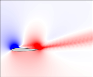
Figure 7. Buffet (a–c) and wake (d–f) modes from SPOD are shown using contour plots of the pressure field for the NACA0012 aerofoil at  $Re = 5\times 10^4$, $\alpha = 0^\circ$ and (a,d) $M = 0.8$, (b,e) $M = 0.75$ and (c,f) $M = 0.72$.
The pressure fields of the wake modes for all  $M$ resemble a von Kármán vortex street pattern. Additionally, pressure waves that originate from near the trailing edge can be observed. The buffet modes for all $M$ also resemble each other. Note that for a type I buffet, the same features seen on the suction side are mirrored on the pressure side, but of opposite sign. Focusing on the suction side, it is seen that the pressure reduction above the aerofoil (large blue region) is coupled with a pressure increase in a small region in the wake (narrow red stripe). This spatial structure is an essential characteristic of transonic buffet as discussed later in § 5.1. Thus, in addition to the similarity in frequency, it is seen that the spatial structure of the coherent oscillations is qualitatively similar under visual inspection (a quantitative description of this similarity is provided in § 5.2) irrespective of whether the flow is transonic or not, corroborating previous conclusions. We also note that while the symmetric NACA0012 aerofoil is the focus of this study (motivated by results reported in Bouhadji & Braza Reference Bouhadji and Braza2003; Jones et al. Reference Jones, Sandberg and Sandham2006), oscillations resembling transonic buffet can also occur for supercritical aerofoils, as shown in Appendix A for Dassault Aviation's V2C aerofoil at $\alpha =0^\circ$. This is seen for the V2C aerofoil for parametric values almost the same as NACA0012 aerofoil and the SPOD modes also have a similar spatial structure.
In summary, self-sustained oscillations at a low frequency of  $St \approx 0.06$ can be observed for the NACA0012 aerofoil at zero incidence for a free-stream Reynolds number of $Re = 50\,000$. These resemble type I transonic buffet, but appear irrespective of whether the flow is transonic or not. Thus, it is established in this section that shock waves are not essential for type I transonic buffet to occur. In conjunction with the result that transonic buffet offset occurs at $M = 0.9$, this implies that shock waves are neither necessary nor sufficient for these oscillations to sustain. Henceforth, we will use ‘transonic buffet’ and ‘transonic-buffet-like oscillations’ (TBLO) to distinguish between cases for which the flow remains always transonic and for which it does not, respectively, and ‘buffet’ to collectively refer to either.
3.2. Effect of spanwise extent
Although transonic buffet on unswept infinite-wing sections is essentially two- dimensional, it has been shown in Zauner & Sandham (Reference Zauner and Sandham2020) that the spanwise width can have a significant effect on its amplitude (but not frequency). Motivated by this, we examined the amplitudes of the TBLO that occur at  $M = 0.75$ for wider spanwise widths of $L_z = 0.1$, 0.25, 0.5 and 1. A similar study for transonic buffet at $M = 0.8$ is presented in Appendix B. The temporal variation of the lift coefficient and its PSD are shown in figure 8. The Strouhal number and the power spectral densities of the peaks in the spectra (buffet and wake modes denoted by subscripts ‘ $b$’ and ‘ $w$’) are also documented in table 3. The effect of $L_z$ on both $St_b$ and $St_w$ is negligible. However, the spanwise width has a strong effect on the amplitude of the oscillations, with the sharpest drop observed when $L_z$ is doubled from 0.05 to 0.1. A further increase in $L_z$ leads to smaller reductions in the amplitude, although sinusoidal oscillations are evident for all cases examined, including $L_z = 1$ (grey curve). Note that for all cases, there are variations in the amplitudes between buffet cycles (i.e. irregular cycles), although the oscillations are persistent.

Figure 8. (a) Temporal variation of lift coefficient past transients and (b) PSD of its fluctuating component as a function of the Strouhal number for the NACA0012 aerofoil at  $Re = 5\times 10^4$, $\alpha = 0^\circ$ and $M = 0.75$ for different spanwise domain widths. Circles and diamonds highlight the buffet and wake mode Strouhal numbers, respectively.
Table 3. Comparison of buffet and wake mode features for  $M = 0.75$, $\alpha = 0^\circ$, $Re = 5\times 10^4$ and different spanwise widths for the NACA0012 aerofoil (all cases reported in § 3.2).

Examining the spatio-temporal flow field in the  $x$–
$x$– $y$ plane, it was found that TBLO features are qualitatively similar for all $L_z$ (see supplementary movie 6 for the case $L_z = 1$). The SPOD spectra were also found to be similar, with peaks present at buffet and wake mode frequencies (not shown for brevity). The spatial features of these modes are shown for a few select cases in figure 9 and can be seen to be qualitatively similar. Overall, the only major difference observed was that, unlike the case of $L_z = 0.05$, where the flow has a small supersonic region in the high- and low-lift phases (see white curve highlighting sonic line in figure 4b,e), the flow remains subsonic at all times for wider domains (see movie 6). Thus, the conclusion that TBLO can be sustained in the subsonic regime holds true even for the largest span considered. Nevertheless, these results suggest that the spanwise extent somehow plays a crucial role in determining buffet amplitude. This is further confirmed by examining the mean flow features. The time- and span-averaged pressure and skin-friction coefficients are compared for different $L_z$ in figure 10. It can be inferred from these plots that the mean flow is not significantly altered by the variation in spanwise width, even for the cases of $L_z = 0.05$ and $L_z = 0.1$ for which the PSD changes by a factor of approximately four. Assuming that buffet arises as a global instability (Crouch et al. Reference Crouch, Garbaruk and Magidov2007), this implies that the growth and/or saturation features of this instability are strongly affected by the spanwise width. This trend is also observed in the presence of shock waves (i.e. type I transonic buffet), as shown in Appendix B. However, these results cannot be generalized – for type II transonic buffet on the supercritical V2C aerofoil, Zauner & Sandham (Reference Zauner and Sandham2020) showed that amplitudes of oscillations increase with an increase in span, which is opposite to the trend observed here.

Figure 9. Buffet (a–c) and wake (d–f) modes from SPOD are shown using contour plots of the pressure field for the NACA0012 aerofoil at  $Re = 5\times 10^4$, $\alpha = 0^\circ$ and $M = 0.75$ for (a,d) $L_z = 0.1$, (b,e) $L_z = 0.5$ and (c,f) $L_z = 1$.

Figure 10. Time- and span-averaged (a) pressure coefficient and (b) skin-friction coefficient variation along the aerofoil surface for the NACA0012 aerofoil,  $Re = 5\times 10^4$ and $\alpha = 0^\circ$, $M = 0.75$ and different domain widths. Here $\bar {C}_f = 0$ is highlighted using a dashed line in (b).
Although the imposition of periodic boundary conditions in the spanwise direction can artificially confine the flow, nevertheless, it provides a controlled numerical experiment that highlights the crucial role that three-dimensional features can play in determining buffet amplitude. This effect could arise from span-varying disturbances affecting boundary layer or wake transition characteristics, but the connection is not obvious. Further analysis towards understanding this effect is required, but we have restricted the scope of this study so as to focus on exploring the links between TBLO and transonic buffet.
4. The link between transonic buffet and LFO
The results at  $\alpha = 0^\circ$ and $Re = 5\times 10^4$ discussed in the preceding section establish the link between type I transonic buffet and TBLO at subsonic conditions without shock waves. In §§ 4.1 and 4.2, we extend this link to incompressible LFO and type II transonic buffet by additionally varying $\alpha$ and $Re$, respectively.
4.1. Link between type I transonic buffet and LFO
The results at  $\alpha = 0^\circ$ and $Re = 5\times 10^4$ discussed in the preceding section establish the link between type I transonic buffet and TBLO. To extend this further and relate with LFO that occur in the incompressible regime (i.e. low $M$) and close to stall (i.e. high $\alpha$), the $\alpha -M$ parameter space is further explored here by both increasing $\alpha$ and decreasing $M$ simultaneously at this $Re$ so as to remain in the narrow range where buffet occurs. It is emphasised that each simulation is performed with the same type of initial conditions of uniform flow and constant boundary conditions and incidence angle (i.e. this is not a hysteresis study). The incidence angles considered are $0^\circ$ to $8^\circ$ in steps of $2^\circ$, and additionally, $\alpha = 9.4^\circ$. For each $\alpha$, the free-stream Mach number required for the simulation was estimated based on the oscillation features observed at lower $\alpha$. Due to the numerical expense involved, no attempts were made to further vary $M$ at a given $\alpha$ as long as sustained oscillations were present at the estimated $M$. Also, based on the results reported in the previous section on domain extent, $L_z = 0.1$ was chosen for all the simulations in this section as a compromise between accuracy and numerical expense (see figure 8 and table 3). All cases reported in this section and their buffet characteristics are summarised in table 4.
Table 4. Comparison of buffet and wake mode features for  $L_z = 0.1$, $Re = 5\times 10^4$ and different ( $M,\alpha$) for the NACA0012 aerofoil (all cases considered in § 4.1; case, $\alpha = 0^\circ$, $M = 0.75$, included for reference).

The lift variations for a few of these cases are shown in figure 11(a,c,d). The variations are strongly irregular and this can make it difficult to discern if buffet occurs. Even for the case of  $\alpha = 9.4$ and $M = 0.3$ (black curve) for which buffet can be visually inferred, there are periods when these oscillations at a low frequency are almost completely damped out, as seen, for example, in $100 \leq t-t_0 \leq 150$. However, these oscillations recover and remain persistent at later times of $t > 150$. The power spectral densities of lift fluctuations for all cases studied are shown in figure 11(b). A case at zero incidence ( $M=0.75$, $L_z = 0.1$, discussed in § 3.2) is additionally provided for reference. It is evident that there are peaks in the spectra at a low frequency (highlighted by circles) indicating buffet for all cases, although there is variability in both $St_b$ and PSD $_b$. Unlike the monotonic increase in $St_b$ seen in § 3.1 when only $M$ is varied, the variation here does not have any specific trend. This is because although $M$ is increased, $\alpha$ is reduced simultaneously and transonic-buffet frequency can vary in a non-monotonic fashion when $\alpha$ is changed (cf. Moise et al. Reference Moise, Zauner and Sandham2022a, figure 17b). Similarly, note that the buffet amplitude at a given $\alpha$ has a nonlinear variation with $M$ (given that it is negligible at onset and offset values of $M$). Thus, monotonic trends in the frequency or amplitude of buffet are not expected when both $M$ and $\alpha$ are varied simultaneously. As shown later, SPOD confirms that the spatial structure of the modes associated with these peaks is consistent and that the modes are correlated (see figure 13 and § 5.2). Note that, unlike the zero incidence case, there is no discrete peak associated with a wake mode for the others. Instead, there is a broadband bump in the spectra centred about $St \approx 1$. A similar bump associated with wake modes is commonly reported for transonic buffet at non-zero incidences e.g. Moise et al. Reference Moise, Zauner and Sandham2022a). Shock waves were absent in the flow field for all non-zero incidence angles studied, implying that the sustained oscillations can be categorised as TBLO for these cases. For the cases considered in this section, when $\alpha \geq 4^\circ$, the energy content on the suction side was dominant and, thus, these cases will also be referred to as type II TBLO.

Figure 11. (a,c,d) Temporal variation of lift coefficient past transients for  $M = 0.7$, $\alpha = 2^\circ$ (a), $M = 0.5$, $\alpha = 6^\circ$ (c) and $M = 0.3$, $\alpha = 9.4^\circ$ (d), and (b) PSD of its fluctuating component as a function of the Strouhal number, $St$ when $\alpha$ and $M$ varied simultaneously at $Re = 5\times 10^4$ for the NACA0012 aerofoil.
Contours of time- and span-averaged local Mach number,  $\bar {M}_{loc}$, are shown for the cases of $\alpha = 8^\circ$, $M = 0.4$ and $\alpha = 9.4^\circ$, $M = 0.3$ in figure 12. The maximum $\bar {M}_{loc}$ attained is 0.65 for the former and 0.51 for the latter and most regions of the flow are found to have $\bar {M}_{loc} \leq 0.4$ for the latter case. Thus, it can be inferred that compressibility effects are insignificant in most of the flow field, especially when $\alpha = 9.4^\circ$ and $M = 0.3$. Although the requirement for a reduced time step prevented exploration at even lower $M$, the present trend of sustained oscillations occurring for decreasing maximum values, $\max (\bar {M}_{loc})$, with increasing $\alpha$ and decreasing $M$ suggests that these oscillations can also sustain in the incompressible regime. The peak in the spectrum for the lowest $M$ simulated occurs at a frequency similar to those reported in experiments studying LFO. For example, Rinoie & Takemura (Reference Rinoie and Takemura2004) reported $St_h = 0.008$, where $St_h$ is the Strouhal number based on the projected height ( $h = c\sin \alpha$) and free-stream velocity. This result is for the NACA0012 profile at $Re = 1.3\times 10^5$ for $M \ll 0.3$ and is of the same order of magnitude as seen in the present study, with $St_h = St\times \sin \alpha \approx 0.005$ for $Re = 5\times 10^4$, $M = 0.3$ and $\alpha = 9.4^\circ$. Thus, we will also refer to the oscillations occurring at the lowest $M$ simulated in the present study as LFO.

Figure 12. Contours of  $\bar {M}_{loc}$ for the NACA0012 aerofoil at $Re = 5\times 10^4$ and (a) $\alpha = 8^\circ$, $M = 0.4$ and (b) $\alpha = 9.4^\circ$, $M = 0.3$.
The SPOD modes associated with the low-frequency peaks are shown in figure 13 for the higher incidences simulated. Additionally, an animation showing the temporal variation of the SPOD mode is provided for the highest incidence simulated (supplementary movie 7). The spatial structure for all cases visually resembles that of type II transonic buffet. A closer look shows that they are also qualitatively similar to the type I buffet modes shown previously (cf. figure 7) when the suction side's features alone are considered. That is, for the present modes, a reduction of pressure on the fore part of the aerofoil (blue region) is coupled with an increase in pressure in the aft part, which extends into the wake (red region). The parametric variation indicates that the extent of the blue region spreads closer to the trailing edge as  $\alpha$ is reduced. For the type I modes at zero incidence, the blue region extends to the trailing edge, but the wake region (red) is similar to that seen here. A quantitative comparison that shows the strong correlation between the buffet modes for different cases and the out-of-phase features of these zones is provided later in § 5.2.

Figure 13. Buffet modes from SPOD are shown using contour plots of the pressure field for the NACA0012 aerofoil at  $Re = 5\times 10^4$ and (a) $\alpha = 6^\circ$, $M = 0.5$, (b) $\alpha = 8^\circ$, $M = 0.4$ and (c) $\alpha = 9.4^\circ$, $M = 0.3$.
In summary, these results demonstrate that both buffet frequency and spatio-temporal modal features (based on SPOD) are essentially the same for type I transonic buffet ( $\alpha = 0^\circ$ and $M = 0.8$), TBLO (all cases considered in the current section) and LFO ( $\alpha = 9.4^\circ$ and $M = 0.3$). Furthermore, the results directly link these phenomena by showing that TBLO can be sustained for intermediate values of $\alpha$ and $M$ by reducing $M$ appropriately when increasing $\alpha$. We again emphasise that these low-frequency TBLO are distinct from vortex shedding (i.e. wake modes). The latter accompanies TBLO for all the cases studied, but at a higher frequency (bump in spectra at $St \approx 1$) and is not the focus of this study.
4.2. Link between type II transonic buffet and LFO
Type II transonic buffet, with shock waves occurring and oscillating exclusively on the suction side, has been the focus of most recent studies, and in this section we try to establish links between this type and TBLO. Note that type II transonic buffet is not observed for any of the cases simulated at  $Re = 5\times 10^4$. This is because offset conditions of type II TBLO and fully stalled conditions occur for $M$ below those at which shock waves appear. To link the type II TBLO observed at $\alpha = 4^\circ$ and $M = 0.7$ at this $Re$ with type II transonic buffet, a few more cases were simulated at higher $Re$. This is motivated by the observation in Zauner & Sandham (Reference Zauner and Sandham2018) that transonic buffet onset and offset can also occur with changes in $Re$. Grid requirements can vary significantly as $Re$ is increased and can lead to large computational expenses. Due to limited resources, it was not possible to explore the parametric space using small changes in values as done in previous sections and only two additional cases are considered here. Nonetheless, observed trends comply well with those seen in previous studies.
The parameters for the two additional cases simulated for which buffet occurs are  $\alpha = 4^\circ$, $M = 0.75$ and $Re = 5\times 10^5$, and $\alpha = 6^\circ$, $M = 0.75$ and $Re = 1.5\times 10^6$ (see table 5). We will refer to these two as high- $Re$ cases. The parametric values associated with these cases were found by trial and error since type II transonic buffet occurs only in a narrow range of the parametric space. For these high- $Re$ cases, the grid used has the same distribution in the $x$–
$x$– $y$ plane as grid 1. However, the spanwise grid spacing is halved to $\Delta z = 0.001$ to account for the increased $Re$. Considering the numerical expense, the narrower span of $L_z = 0.05$ is used. We emphasise that this configuration ( $Re$,
$Re$,  $L_z$ and $\Delta z$) is similar to that used in a majority of simulations carried out in our previous studies (Moise et al. Reference Moise, Zauner and Sandham2022a,Reference Moise, Zauner, Sandham, Timme and Heb; Zauner et al. Reference Zauner, Moise and Sandham2023), and for which various validations and verification have been performed with LES, DNS and experiments (see § 2).
Table 5. Comparison of buffet and wake mode features for the NACA0012 aerofoil (all cases considered in § 4.2; case,  $\alpha = 4^\circ$, $M = 0.7$, $Re = 5\times 10^4$, $L_z = 0.05$, included for reference).

The variation of the lift coefficient and the PSD of its fluctuating component are shown in figure 14 for the three different  $Re$ examined. In contrast to the irregular temporal variation of the lift coefficient observed at subsonic conditions ( $Re = 5\times 10^4$), the high- $Re$ cases, for which the flow is transonic, exhibit a more regular temporal variation. The oscillation cycles for the latter are also dominated by the low-frequency content, as can also be inferred from the power spectra. A strong increase in the buffet frequency with $Re$ can be observed, from $St_b \approx 0.03$ at $Re = 5\times 10^4$ to $St_b \approx 0.12$ at $Re = 5\times 10^5$ and $St_b \approx 0.15$ at $Re = 1.5\times 10^6$. Note that it is not only $Re$ that is increased between cases, but also $M$ (or $\alpha$), and the latter can have a strong influence in increasing $St_b$ (e.g. figure 3a here and figure 8 in Zauner et al. Reference Zauner, Moise and Sandham2023).

Figure 14. (a,c,d) Temporal variation of lift coefficient past transients for the NACA0012 aerofoil at  $Re$,
$Re$,  $\alpha$ and $M$ of $5\times 10^4$, $4^\circ$ and $0.7$ (a), $5\times 10^5$, $4^\circ$ and $0.75$ (c), $1.5\times 10^6$, $6^\circ$ and $0.75$ (d). (b) Power spectral density of its fluctuating component as a function of the Strouhal number, $St$ when $Re$ is also varied.
The streamwise density gradient fields in the high- and low-lift phases are compared in figure 15. The presence of shock waves that exhibit a fore–aft motion on the suction surface can be inferred for the high- $Re$ cases. Thus, these two cases can be considered as examples of type II transonic buffet. We note that there are strong temporal variations in the boundary layer separation location between the high- and low-lift phases. This periodic fore–aft motion of the separation point is a characteristic feature of transonic buffet (see figure 18 in Moise et al. Reference Moise, Zauner, Sandham, Timme and He2022b) and further corroborates the conclusion that it is linked with LFO, which has been described as involving a quasi-periodic switching between stalled and unstalled conditions (Zaman et al. Reference Zaman, McKinzie and Rumsey1989).

Figure 15. Streamwise density gradient contours on the  $x$–
$x$– $y$ plane shown at the approximate (a–c) high- and (d–f) low-lift phases of the low-frequency cycle for the NACA0012 aerofoil at (a,d) $\alpha = 4^\circ$, $M = 0.7$, $Re = 5\times 10^4$; (b,e) $\alpha = 4^\circ$, $M = 0.75$, $Re = 5\times 10^5$ and (c,f) $\alpha = 6^\circ$, $M = 0.75$, $Re = 1.5\times 10^6$. The sonic line is highlighted using a white curve.
The buffet modes obtained from SPOD are compared in figure 16 for all cases. Comparing the cases of the lowest two  $Re$ considered, the spatial structure of the modes appear similar under visual inspection, with a pattern of pressure reduction (blue) on the suction surface accompanying a pressure increase (red) near the trailing edge and the wake (see § 5.2 for quantitative comparisons). This pattern is qualitatively the same as that seen for LFO in figure 13, except that the region associated with the pressure reduction extends further downstream here. For the highest $Re$, the buffet mode is similar to the other cases except for the presence of a small region associated with a pressure increase on the suction side. However, the animation provided for the spatio-temporal mode (supplementary movie 8) shows that the spatial structures are closer at other time instants in the buffet cycle. This suggests that the choice of using the high-lift phase as the reference phase to compare modes from different cases is not always ideal, but sufficient to establish their similarities. This is confirmed by choosing a different reference phase and comparing the instantaneous features in figure 17. Here, the reference phase is chosen such that the pressure (from SPOD) on the upper corner of the blunt trailing edge is real-valued, which is similar to the approach adopted in Moise et al. (Reference Moise, Zauner, Sandham, Timme and He2022b).

Figure 16. Buffet modes from SPOD for the NACA0012 aerofoil are shown using contour plots of the pressure field for cases (a)  $\alpha = 4^\circ$, $M = 0.7$, $Re = 5\times 10^4$; (b) $\alpha = 4^\circ$, $M = 0.75$, $Re = 5\times 10^5$ and (c) $\alpha = 6^\circ$, $M = 0.75$, $Re = 1.5\times 10^6$. The comparison is done by choosing the instant where the high-lift phase occurs as the reference phase.

Figure 17. Buffet modes from SPOD for the NACA0012 aerofoil are shown using contour plots of the pressure field for cases (a)  $\alpha = 4^\circ$, $M = 0.7$, $Re = 5\times 10^4$; (b) $\alpha = 4^\circ$, $M = 0.75$, $Re = 5\times 10^5$ and (c) $\alpha = 6^\circ$, $M = 0.75$, $Re = 1.5\times 10^6$. The comparison is done by choosing the reference phase such that the pressure at the upper corner of the blunt trailing edge is real-valued.
5. Discussion
5.1. Link with other studies
The results from the preceding section suggest that LFO and type II transonic buffet are qualitatively similar based on a visually identifiable pattern in SPOD modes and trends in frequency for the symmetric NACA0012 aerofoil under conditions of free transition at low  $Re$. However, most recent studies focus on type II transonic buffet on supercritical aerofoils for forced-transition conditions and high $Re$ (Giannelis et al. Reference Giannelis, Vio and Levinski2017). To generalize the link between the two flow phenomena, we compare features of LFO to those of type II transonic buffet from our previous studies where we have examined supercritical aerofoils at a variety of flow conditions. Note that these include cases with turbulent or laminar transonic buffet, with multiple shock waves or a single shock wave present. We consolidate these results on buffet mode features here so that a link between a typical transonic-buffet mode and LFO can be established. However, to be consistent, we have presented here the buffet mode features at the phase when the lift induced is maximum. This differs from the plots shown in previous studies, as they are for a different phase of the buffet cycle, based on features at the trailing edge.
We start with figure 18(a), where the dominant unstable mode obtained from a global linear stability analysis of results based on a RANS framework is shown. The results are for flow over ONERA's OAT15A aerofoil at  $\alpha = 3^\circ$ for $M = 0.74$, $Re = 3\times 10^6$ and fully turbulent conditions. These results for type II turbulent transonic buffet were originally presented in Moise et al. (Reference Moise, Zauner, Sandham, Timme and He2022b). Note that this supercritical OAT15A aerofoil has been extensively studied for similar flow conditions in various studies (Sartor et al. Reference Sartor, Mettot and Sipp2015; Fukushima & Kawai Reference Fukushima and Kawai2018; Garbaruk et al. Reference Garbaruk, Strelets and Crouch2021). The SPOD mode at buffet frequency obtained from LES of flow around ONERA's laminar OALT25 profile at $\alpha = 4^\circ$ for $M = 0.735$, $Re = 3\times 10^6$ and free-transition conditions is shown in figure 18(b). These results on type II laminar transonic buffet were originally presented in Zauner et al. (Reference Zauner, Moise and Sandham2023) and these flow conditions have also been studied using LES in Dandois et al. (Reference Dandois, Mary and Brion2018) and experiments in Brion et al. (Reference Brion, Dandois, Mayer, Reijasse, Lutz and Jacquin2020). The SPOD mode at buffet frequency obtained from LES of flow around Dassault Aviation's laminar V2C profile at $\alpha = 5^\circ$ for $M = 0.735$, $Re = 5\times 10^5$ and forced-transition conditions is shown in figure 18(c). This is based on the results of type II turbulent transonic buffet presented in Moise et al. (Reference Moise, Zauner, Sandham, Timme and He2022b), where boundary layer transition to turbulence was triggered at $x = 0.2$ on the suction side using a synthetic unsteady jet.

Figure 18. Buffet modes for (a) OAT15A, fully turbulent conditions,  $\alpha = 3^\circ$, $M = 0.74$, $Re = 3\times 10^6$, based on global linear stability analysis, and rest, based on SPOD; (b) OALT25, free transition, $\alpha = 4^\circ$, $M = 0.735$, $Re = 3\times 10^6$; (c) V2C, forced transition (using a trip on the suction side at $x = 0.2$), $\alpha = 5^\circ$, $M = 0.735$, $Re = 5\times 10^5$; (d) same as (b), but with $Re = 5\times 10^5$; (e) same as (c), but for free-transition conditions; and (f) NACA0012, $\alpha = 9.4^\circ$, $M = 0.3$, $Re = 5\times 10^4$. The data for (a,c,e) are from Moise et al. (Reference Moise, Zauner, Sandham, Timme and He2022b), (b,d) from Zauner et al. (Reference Zauner, Moise and Sandham2023), whereas (f) is from the present study.
These three cases were all found to contain a single shock wave in the flow field that exhibited a fore–aft motion of small amplitude ( $\Delta x < 0.1$). Two zones of importance that are common to all three cases are marked as Z1 and Z2. The former (blue region) is present above the suction side close to the mid-chord and is concentrated around the mean shock location. The latter (red region, i.e. out of phase with Z1) occurs in the vicinity of the trailing edge and extends into the wake. In addition to these two prominent zones, another small zone of increased pressure near the shock at the current phase, i.e. the unmarked red region at the shock foot that is bounded by Z1, can be identified. However, this zone might not be always visible as larger shock wave excursions could lead to Z1 masking this region. This is likely the case in figure 7(a) in Fukushima & Kawai (Reference Fukushima and Kawai2018) and for the remaining cases considered. The other cases shown (figure 18d,e) are the SPOD modes associated with type II laminar transonic buffet for the OALT25 and V2C for the same respective flow conditions as that discussed before, but for a lower $Re = 5\times 10^5$ for the former (i.e. $\alpha = 4^\circ$, $M = 0.735$ and free transition) and for free-transition conditions for the latter (i.e. $\alpha = 5^\circ$, $M = 0.735$ and $Re = 5\times 10^5$). These two cases are characterised by multiple shock waves that exhibit large-amplitude streamwise oscillations ( $\Delta x \geq 0.1$). The zones, Z1 and Z2, can also be discerned here, although, in contrast to the previous cases, Z1 is not concentrated but extends over almost the entire suction surface due to the large-amplitude excursions associated with multiple shock waves.
Finally, when comparing the SPOD mode of LFO obtained in this study at  $\alpha = 9.4^\circ$, $M = 0.3$, $Re = 5\times 10^4$ for the NACA0012 aerofoil at free-transition conditions (figure 18f), for which the flow remains essentially incompressible, the similarity is evident, with both Z1 and Z2 clearly identifiable, albeit with the extent of Z2 now extending upstream up to mid-chord. Thus, while the visual similarities between the global mode associated with transonic buffet on the commonly studied OAT15A aerofoil and the SPOD mode associated with LFO in the present study might not be immediately apparent, examining the sequence of plots shown in figure 18 indicates that the spatial structure of these two modes have a common pattern (see also, § 5.2 and table 8). It consists of an out-of-phase coupling between a region upstream in the fore part of the aerofoil with a region located downstream in the aft part and extending into the wake. This pattern is clearly distinct from that of the wake mode that is seen to accompany buffet in the present study (figure 9d–f) or the incompressible 2-D wake-instability mode reported in § 4.1.4 in Plante et al. (Reference Plante, Dandois, Beneddine, Laurendeau and Sipp2020). The latter two modes instead resemble a von Kàrmàn vortex street. It is also interesting to note that zones Z1 and Z2 are present even in three-dimensional transonic-buffet cells that occur over wings or swept infinite-wing sections (e.g. Crouch et al. Reference Crouch, Garbaruk and Strelets2019) and that these modes too have shown to have an analogous incompressible instability with visibly similar patterns, i.e. stall cells (Plante et al. Reference Plante, Dandois, Beneddine, Laurendeau and Sipp2020).
When considering this result in conjunction with the results that the frequencies of the two phenomena are close ( $St \approx 0.1$ for the OAT15A case and $St \approx 0.033$ for LFO observed here) and the links provided in preceding sections (§§ 4.1 and 4.2), we conclude that LFO and transonic buffet on aerofoils have similar characteristics and, thus, their sustenance is likely to be driven by similar physical mechanisms.
As noted in § 1, the results from previous studies show that both flow phenomena occur as global linear instabilities (Crouch et al. Reference Crouch, Garbaruk and Magidov2007; Iorio et al. Reference Iorio, González and Martínez-Cava2016; Busquet et al. Reference Busquet, Marquet, Richez, Juniper and Sipp2021) and are associated with periodic boundary layer separation and reattachment (i.e. switching between stalled and unstalled states), which further corroborate this conclusion. It is also interesting to note that in flight tests, buffet onset occurs during manoeuvres such as turns and pull-ups for flight Mach numbers in the range 0.1 to 0.8 (e.g. figure 4 in Huston & Skopinski Reference Huston and Skopinski1951 and figure 1 in Purser & Wyss Reference Purser and Wyss1951). This buffet boundary varies continuously in plots of normal coefficient versus flight Mach number as the latter changes from subsonic to transonic regimes (referred to as stall and shock regimes), which is consistent with the present results. However, since it drops relatively steeply in the latter regime, it has been suggested that ‘Along the steep portion of the boundary the buffeting is thought to be primarily due to compressibility rather than to reaching the stall as in the low Mach number portion of the boundary’ (Purser & Wyss Reference Purser and Wyss1951). However, the present results suggest that variations in steepness might be a quantitative feature but that buffet's spatio-temporal features would still be qualitatively the same at all Mach numbers.
5.2. Quantitative comparisons
In previous sections, the SPOD buffet modes have been suggested to represent the same phenomenon based on topographical similarities. That is, a visual examination of the buffet modes reveals the presence of zones Z1 and Z2 that are out of phase with each other. A quantitative comparison between buffet modes obtained at different conditions is not easy, since the streamwise location of these zones, their extent and shape change widely with flow parameters. Although pattern recognition algorithms using unsupervised learning approaches can be used to make global comparisons in future studies, given their complexity, we have adopted two relatively simple approaches in the present study, involving global and local correlations. In the first approach we make a global comparison of the SPOD pressure fields by computing a correlation coefficient based on a spatial inner product, given by
 \begin{equation} C(\,p_1,p_2) = \left|\frac{\int_\varOmega p_1^* W p_2 \,{\rm d}\varOmega}{\sqrt{\int_\varOmega p_1^* W p_1 \,{\rm d}\varOmega \int_\varOmega p_2^* W p_2\, {\rm d}\varOmega}}\right|, \end{equation}
where  $p_1$ and $p_2$ represent the complex spatial pressure fields associated with the two SPOD modes being compared, $W$ is the weight associated with the inner product on the spatial domain, $\varOmega$, and $p^*$ represents the complex conjugate of $p$. The weight matrix is computed using the approach mentioned in § 2.3. Since different grids are used at different incidence angles, linear interpolation was used when required to compute the variables on the grid points associated with grid 0 (at zero incidence). The correlation coefficient computed is expected to be only useful as a similarity measure between two SPOD modes associated with cases related by an incremental change in the parameters (e.g. between results from cases of $M = 0.75$ and $M = 0.8$ in § 3.1, with other parameters fixed at $\alpha = 0^\circ$, $Re = 5\times 10^4$). This is because the global variation between the modes is expected to be relatively low only for such cases. By contrast, factors mentioned above such as variations in mean location, extent and shape of zones Z1 and Z2 are expected to lead to large quantitative variations when parametric differences are large (e.g. between the case for which $\alpha = 9.4^\circ$, $M = 0.3$ and that for which $\alpha = 0^\circ$, $M = 0.75$ in § 4.1). The correlation coefficient for pairs of buffet modes with minimal changes in parameters is presented in table 6. It is seen that for the cases simulated in § 3.1, where only $M$ is varied whilst other parameters remain the same ( $\alpha = 0^\circ$ and $Re = 5\times 10^4$), the correlations between the buffet modes are strong. For cases in § 4.1, the correlation coefficient is reasonably high considering that two parameters, $\alpha$ and $M$, are simultaneously varied between cases. The correlations are also relatively lower at low angles of attack as increasing the angle of attack leads to reduced activity in the pressure side of the aerofoil, as buffet transitions from type I to type II. The correlations are lowest when comparing the cases of $Re = 5\times 10^4$, $M = 0.7$ and $Re = 5\times 10^5$, $M = 0.75$, which could possibly be because of the large change in $Re$ for these cases and because of the variation in buffet amplitude, the latter affecting the errors in the SPOD approach. This requires further scrutiny with results at intermediate values of parameters that have not been pursued due to limitations on computational resources. However, it was found that the values of these correlations are an order of magnitude higher than that of the correlation between the wake mode and the buffet mode. This is detailed for a few cases in table 7 and confirms quantitatively the visually stark differences between the wake and buffet modes.
Table 6. Correlation coefficient computed for SPOD pressure fields (buffet modes) based on different pairs of cases simulated in this study (only parameters required to identify a case are provided; see table 1 or tables at the start of the corresponding section for more details).

Table 7. Correlation coefficient computed for SPOD pressure fields comparing wake and buffet modes for a few cases simulated (only parameters required to identify a case are provided; see table 1 or tables at the start of the corresponding section for more details).

In the second approach to quantify the similarity between SPOD modes, we find a local correlation between modes based on phase differences at representative points in zones Z1 and Z2 (see figure 18). This approach has the advantage over the previous approach in that it can account for changes in the mean flow and the distortions in the mode shapes with changing flow parameters. Since zone Z1 occurs on the aerofoil's suction surface and zone Z2 is associated with the near wake, we divide the SPOD domain into two regions with approximate boundaries,  $0.1 \leq x' \leq 0.8$ and $1 \leq x' \leq 1.2$, respectively, and for the upper part of the aerofoil. Noting that the SPOD mode gives a complex field with each point having a magnitude and phase associated with it, we develop a procedure to quantify the phase difference between these two regions as follows. A grid point representative of each region is chosen by finding that location where the magnitude of the pressure (from the complex SPOD buffet mode) is maximum over the entire region. These points, denoted in a chordwise coordinate system as $(x_1',y_1')$ and $(x_2',y_2')$, are expected to be representative of Z1 and Z2, respectively. The phase difference in pressure from the SPOD buffet mode between the two spatial points is then computed as
 \begin{equation} \Delta \phi = \phi({x_1',y_1'})-\phi({x_2',y_2'}), \end{equation}
where  $\phi$ is the phase of the complex SPOD pressure field at the points where the maximum is achieved, defined as
 \begin{equation} (x_1',y_1') = \big\{(x',y') \mid \max_{Z1} p(x',y')\big\}\!, \quad (x_2',y_2') = \big\{(x',y') \mid \max_{Z2} p(x',y')\big\}\!. \end{equation}
 The computed variables for the different cases studied are documented in table 8. Note that for the case of the OAT15A, the results are based on the dominant unstable mode from a global linear stability analysis of results from RANS simulations and not from SPOD. The quantitative matches appear reasonable with the phase difference ranging between  $136^\circ \leq \Delta \phi \leq 181^\circ$, indicating that these two points are approximately out of phase with each other. Other arbitrarily chosen pairs of points in these two regions (with the only requirement that the magnitude of the pressure is relatively negligible) also had phase differences in the same range, indicating that there are two global regions, Z1 and Z2, which are present for these cases, albeit with variations in their extent and shape.
Table 8. Locations of maximum SPOD pressure magnitude in regions above the aerofoil and in the near wake and the phase difference between these points. These are computed based on the buffet SPOD mode for various cases discussed in different sections of this paper (only parameters required to identify a case are provided, see table 1 or tables at the start of their corresponding sections for more details). The case of OAT15A is based on the dominant unstable mode from a global linear stability analysis of RANS results instead of SPOD from LES results.

5.3. Possible implications for buffet on aerofoils
There are several important consequences to the hypothesis that transonic buffet and LFO are linked and that buffet-like oscillations can occur even in the absence of shock waves. Firstly, many proposed physical models for transonic buffet require the presence of a shock wave. For example, the popular model proposed in Lee (Reference Lee1990) for type II transonic buffet assumes that waves that are generated at the shock foot travel downstream within the boundary layer and interact with the trailing edge, leading to the development of ‘Kutta’ waves that then propagate upstream in the potential flow region and interact with the shock waves. The model then predicts buffet frequency based on the distance the waves travel, which is approximated as that between the shock wave and the trailing edge, which cannot be computed if no shock wave is present. Equivalent drawbacks also arise for other models that are similar to that of Lee such as those proposed in Jacquin et al. (Reference Jacquin, Molton, Deck, Maury and Soulevant2009) and Hartmann, Feldhusen & Schröder (Reference Hartmann, Feldhusen and Schröder2013) for type II transonic buffet and that proposed in Gibb (Reference Gibb1988) to explain type I transonic buffet. Thus, we suggest that an acoustic wave-propagation-based feedback model for transonic buffet must be discarded or substantially modified to explain oscillations seen at subsonic and incompressible conditions.
Any improved model of buffet needs to recognise that the phenomenon can arise with or without shock waves. In this context, the LFO has been previously observed (Sandham Reference Sandham2008) to be sustained based only on boundary layer integral models and potential flow interaction. Hence, both buffet and LFO could be associated with a global instability related to flow separation coupled with the external potential flow that occurs close to stall. Shock waves might then play a role in promoting stall-like conditions, but this is only secondary since stall occurs even in the absence of shock waves and conditions required for the same can be achieved at higher  $\alpha$ by reducing $M$. From this perspective, the success of control strategies using devices such as shock control bumps, vortex generators and trailing edge devices (e.g. Tijdeman & Seebass Reference Tijdeman and Seebass1980; Giannelis et al. Reference Giannelis, Vio and Levinski2017; Caruana et al. Reference Caruana, Mignosi, Corrège, Le Pourhiet and Rodde2005; D'Aguanno, Schrijer & van Oudheusden Reference D'Aguanno, Schrijer and van Oudheusden2023) on affecting buffet could be possibly reinterpreted as due to their effect on the global flow field and especially boundary layer characteristics. Similarly, the results of Paladini et al. (Reference Paladini, Beneddine, Dandois, Sipp and Robinet2019a) and Houtman, Timme & Sharma (Reference Houtman, Timme and Sharma2023) can also be interpreted likewise. These studies have identified the active or wave maker regions for buffet as the shock foot (e.g. see figure 4(c) of the latter study), but this could arise because boundary layer separation occurs at the shock foot and shock waves need not be as consequential as separation for the origins of the instability. Separation can also occur when there is no shock wave (e.g. at high incidence angles) and if it is the key factor, could lead to the buffet instability. Features like the sensitivity of the amplitude to spanwise domain size could then be linked to three-dimensional aspects of either separation or the potential flow response. Further examination is required to confirm this hypothesis, but if true, this would imply that flow control strategies for eliminating/mitigating buffet could shift focus away from only shock waves to a consideration of the whole flow and boundary layer separation and aim at delaying the latter.
6. Conclusions
6.1. Observations
In this study the flow over an infinite-wing section based on the NACA0012 aerofoil profile has been examined for a wide range of flow conditions by performing simulations at various incidence angles, and free-stream Mach and Reynolds numbers. At a low  $Re = 5\times 10^4$ and zero incidence angle, type I transonic buffet, characterised by shock waves oscillating out of phase on both sides of the aerofoil, was observed at high $M$. By decreasing $M$ and keeping other parameters fixed, it was found that oscillations resembling transonic buffet, referred to as TBLO, persist, even though the flow remains subsonic at all times. Extending the span of the domain strongly affected the amplitude of these oscillations, but the frequency was unaffected and the oscillations were sustained for all $L_z$ considered, with the highest simulated being $L_z = 1$. Using SPOD, the coherent spatio-temporal features in the flow field were scrutinised. For all cases, peaks were observed in the SPOD spectra at the buffet frequency. The spatial structure of the SPOD mode at this frequency and a given phase consisted of a zone associated with a pressure reduction on the surface of the aerofoil (Z1) that is accompanied by a zone associated with pressure increase in the near wake of the aerofoil (Z2). This structure was preserved in buffet modes for all cases, irrespective of whether the flow is subsonic or transonic and a correlation coefficient based on a global inner product between buffet modes confirmed that these modes are strongly correlated with each other. These results suggest that shock waves and transonic flow are not necessary for buffet to sustain.
Increasing the incidence angle from  $\alpha = 0^\circ$ while simultaneously reducing $M$, it was observed that buffet sustains, albeit with some variations in frequency and amplitude. However, examining the SPOD modes confirmed that the spatial structure is qualitatively and quantitatively the same on the suction side for all cases. For all SPOD buffet modes, the regions Z1 and Z2 were visually identifiable and had an out-of-phase relation, whilst the correlation coefficient between cases for which the variation in flow parameters is minimal was also sufficiently high. At a high incidence and low free-stream Mach number ( $\alpha = 9.4^\circ$ and $M = 0.3$), compressibility effects were negligible, indicating that the oscillations can also be classified as LFO. Type II transonic buffet was also simulated by choosing higher $Re$,
$Re$,  $M$ and $\alpha$ and linked with buffet at low $Re$, although with only a few cases simulated. Furthermore, using a consistent phase definition, the SPOD modes for LFO have been shown to be similar to the global mode obtained from a linear stability analysis for flow over ONERA's OAT15A aerofoil (exhibiting type II transonic buffet) and other aerofoils and flow-transition conditions from previous studies. For all cases, zones Z1 and Z2 are the dominant spatial features and are clearly identifiable and out of phase with each other, although their spatial location and extent can differ based on the case. More importantly, it is evident that the spatial structure is distinct from the alternating patterns seen in a von Kàrmàn vortex street. All these results indicate that type I and II transonic buffet, type I and II TBLO and LFO, all have a qualitative and quantitative similarity in their spatial structure (SPOD) and frequency ( $St \ll 1$), and that a variation in flow conditions in small steps can be used to link one with the others. Interestingly, the same out-of-phase Z1 and Z2 zones can be identified in three-dimensional transonic-buffet cells (albeit with spanwise variations), and analogous to the present study, the three-dimensional transonic modes have also been linked with three-dimensional stall cells that occur in the incompressible regime (Plante et al. Reference Plante, Dandois, Beneddine, Laurendeau and Sipp2020).
6.2. Interpretations and scope for future studies
Results from the present study suggest that buffet might arise as an instability that occurs due to boundary layer separation and reattachment at conditions close to stall, suggesting that flow separation is more relevant to the fundamental mechanism than shock waves. This hypothesis requires further exploration but, if true, flow control strategies that aim to delay stall could be beneficial in mitigating these oscillations. Further studies on physical mechanisms and control strategies are required to examine these aspects. Two other crucial aspects require further exploration. Firstly, the present conclusions based on SPOD and LES need to be corroborated using global linear stability and resolvent analysis of results from RANS, which can also shed more light on the sensitivity and receptivity of the global modes associated with LFO and transonic buffet. More importantly, it can be inferred from Beneddine et al. (Reference Beneddine, Sipp, Arnault, Dandois and Lesshafft2016) that SPOD modes and globally unstable modes from linear stability analysis need not be the same, especially when sub-dominant modes exist in the spectrum and turbulence can excite such modes. Although Moise et al. (Reference Moise, Zauner, Sandham, Timme and He2022b) have shown that the SPOD and linear stability modes are topologically similar for transonic buffet, the same has not been confirmed for incompressible LFO. However, stability analysis has confirmed that LFO is due to a dominant unstable global mode (Iorio et al. Reference Iorio, González and Martínez-Cava2016; Busquet et al. Reference Busquet, Marquet, Richez, Juniper and Sipp2021) and the other sub-dominant unstable mode that can coexist is the wake mode. Since the wake mode is related to vortex shedding and also coexists independently with transonic buffet, it is likely that it does not affect the SPOD mode associated with LFO either, but this requires confirmation.
Secondly, a direct connection between LFO and transonic buffet for fully turbulent or forced-transition scenarios must be explored. We note that the present study has made direct links between LFO and transonic buffet by varying parameters in small increments only for cases of natural transition at low  $Re$ (i.e. laminar buffet). For this setting, there are multiple shock waves present over a large portion of the aerofoil surface. We have only shown that the spatial structure has similar patterns for the turbulent and laminar cases by comparing with results from other studies (global linear stability analysis and SPOD modes). However, we have not performed an incremental variation of the parameters to connect turbulent transonic buffet with LFO due to numerical expense. This is another avenue for exploration that can shed light on the effect of shock structure on the links between these two phenomena.
Supplementary movies
Supplementary movies are available at https://doi.org/10.1017/jfm.2023.1065. The data that support the findings of this study are openly available in the repository of the University of Southampton at http://eprints.soton.ac.uk/id/eprint/485637.
Acknowledgements
We would like to acknowledge the computational time on ARCHER and ARCHER2 (UK supercomputing facility) provided by the UK Turbulence Consortium (UKTC) through the EPSRC grant EP/R029326/1. The support and the resources provided by PARAM Sanganak under the National Supercomputing Mission, Government of India at the Indian Institute of Technology, Kanpur are gratefully acknowledged. We also acknowledge the use of the IRIDIS High Performance Computing Facility, and associated support services at the University of Southampton, in the completion of this study. The V2C aerofoil geometry was kindly provided by Dassault Aviation. We thank ONERA for the OALT25 and OAT15A geometries. We also thank Dr Timme and Dr Wei for the data on the buffet mode from global linear stability analysis of RANS results (OAT15A). P.M. would like to acknowledge his daughter Vanmati who served as an inspiration for the study.
Funding
This study was funded by the Engineering and Physical Sciences Research Council (EPSRC) grant, ‘Extending the buffet envelope: step change in data quantity and quality of analysis’ (EP/R037167/1).
Declaration of interests
The authors report no conflict of interest.
Appendix A. Results for V2C aerofoil at zero incidence
Type I TBLO were also observed for Dassault Aviation's laminar supercritical V2C aerofoil for  $Re = 5\times 10^4$ and $L_z = 0.05$ (grid 0). Lift characteristics are shown in figure 19 for three different free-stream Mach numbers. While qualitatively similar, there are interesting quantitative differences between these results and those for the NACA0012 aerofoil at $\alpha = 0^\circ$ (cf. figures 2 and 3). The lift oscillations are relatively irregular for the V2C aerofoil (similar to NACA0012 results for $\alpha \neq 0^\circ$), although the amplitude is similar for both aerofoils. The effect of spanwise width on this amplitude was not examined at this $Re$ due to the associated numerical expense (see Zauner & Sandham (Reference Zauner and Sandham2020) for results at a higher $Re$). The buffet frequency (highlighted using circles in the PSD) is also relatively higher, with $St_b \approx 0.15$. This is similar to those reported at higher $Re$ for this aerofoil at zero incidence (e.g. $St_b = 0.13$ (Moise et al. Reference Moise, Zauner and Sandham2022a) at $Re = 5\times 10^5$), implying that the buffet frequency does not change significantly with $Re$ for this aerofoil when $\alpha = 0^\circ$. This should be contrasted with the results presented in § 4.2 where there is a strong variation in the buffet frequency with $Re$ for the NACA0012 aerofoil, albeit at $\alpha = 4^\circ$.

Figure 19. (a) Temporal variation of lift coefficient past transients and (b) PSD of its fluctuating component for different free-stream Mach numbers for the V2C aerofoil at  $Re = 5\times 10^4$ and $\alpha = 0^\circ$. Circles and diamonds highlight $St_b$ and $St_w$, respectively.
Nevertheless, the trend seen for NACA0012 is also observed here, as seen from figure 20 that shows contours of the streamwise density gradient on the  $z = 0$ plane at high- and low-lift phases for the three $M$. At the highest $M = 0.8$, the flow exhibits type I transonic buffet, with multiple shock waves and supersonic regions (delineated by the white isoline) that oscillate on either side of the aerofoil. At the intermediate $M = 0.77$, a small pocket of a supersonic region occurs on the suction/pressure side in the high-/low-lift phase. At the lowest, $M = 0.75$, the flow field is entirely subsonic. Note that the V2C aerofoil is asymmetric, and thus, minor differences exist between the high- and low-lift phases, but there is a close match with trends seen for the NACA0012 aerofoil (e.g. the same trend is observed for the latter aerofoil at $M = 0.8$, 0.75 and 0.72 with other parameters the same). This is further corroborated by the buffet modes shown in figure 21 that also resemble those observed for the NACA0012 aerofoil, albeit with an additional region in the fore part of the aerofoil having an out-of-phase pressure variation with the aft part of the aerofoil. These results suggest that TBLO in the subsonic regime are a generic flow feature and could occur on other aerofoil profiles for similar flow conditions.

Figure 20. Streamwise density gradient contours on the  $x$–
$x$– $y$ plane shown at approximate high-lift (a–c) and low-lift (d–f) phases for $M = 0.8$ (a,d), $M = 0.77$ (b,e) and $M = 0.75$ (c,f), for the V2C aerofoil at $Re = 5\times 10^4$ and $\alpha = 0^\circ$. The sonic line is highlighted using a white curve.

Figure 21. Buffet (a–c) and wake (d–f) modes from SPOD for the V2C aerofoil are shown using contour plots of the pressure field at  $Re = 5\times 10^4$, $\alpha = 0^\circ$ for (a,d) $M = 0.8$, (b,e) $M = 0.77$ and (c,f) $M = 0.75$.
Appendix B. Effect of spanwise extent on type I transonic buffet at  $M=0.8$

The domain width,  $L_z$, has been shown in § 3.2 to strongly influence the buffet oscillations observed at $M = 0.75$, $\alpha = 0^\circ$ and $Re = 5\times 10^4$ for the NACA0012 aerofoil. Note that at this $M$, the flow is only weakly transonic ( $L_z = 0.05$, see figure 4b,e) or entirely subsonic (higher $L_z$, see supplementary material). To see if this effect is also present when shock waves develop in the flow field, a few cases of $L_z > 0.05$ were simulated for $M = 0.8$ where type I transonic buffet with shock waves was observed when $L_z = 0.05$, $\alpha = 0^\circ$ and $Re = 5\times 10^4$ for the NACA0012 aerofoil. The temporal variation of the lift coefficient and its PSD are compared in figure 22 for three different $L_z$. Due to associated numerical expense, other $L_z$ were not attempted. It is evident that the amplitude of the lift fluctuations is almost halved from approximately 0.2 to 0.1 when $L_z$ is doubled from 0.05 to 0.1. Thus, the trend of reducing buffet amplitude as $L_z$ is increased from 0.05 reported for $M = 0.75$ is also observed here. However, when $L_z$ is increased to 0.5, we see that the lift amplitude remains approximately the same implying that the effect of domain width is not significant for $L_z \geq 0.1$. This should be contrasted with the $M = 0.75$ case discussed in § 3.2 where this approximately occurs for $L_z = 1$. Nevertheless, as with that case, the buffet frequency remains approximately the same for all $L_z$.

Figure 22. (a) Temporal variation of lift coefficient past transients and (b) PSD of its fluctuating component as a function of the Strouhal number,  $St$ for $M = 0.8$, $\alpha = 0^\circ$, $Re = 5\times 10^4$ and NACA0012 aerofoil and different spanwise domain widths. Circles and diamonds highlight the buffet and wake mode Strouhal numbers ( $St_b$ and $St_w$), respectively.


 Open access