


1. Introduction
Up to a specific Reynolds number, it is widely believed that the laminar state of most shear flows is unconditionally stable (Reynolds Reference Reynolds1895; Orr Reference Orr1907; Serrin Reference Serrin1959). However, beyond this threshold, the behaviour of the fluid remains an open question.
In the 19th century, Lord Kelvin (F.R.S. Reference Sir W.Thomson L.L.D.1887) suggested that the stability threshold amplitude decreases as viscosity approaches zero: ‘ $\ldots$
the steady motion is stable for any viscosity, however small; and that the practical unsteadiness pointed out by Stokes forty-four years ago and so admirably investigated experimentally five or six years ago by Osbourne Reynolds, is to be explained by limits of stability becoming narrower and narrower the smaller is the viscosity’. Unfortunately, determining this permissible perturbation level of the laminar state has proven to be a challenging problem. One exception is the well-known linear stability limit, beyond which the laminar state’s region of attraction vanishes. However, for several practical applications, this limit is excessively high, if not infinite.
$\ldots$
the steady motion is stable for any viscosity, however small; and that the practical unsteadiness pointed out by Stokes forty-four years ago and so admirably investigated experimentally five or six years ago by Osbourne Reynolds, is to be explained by limits of stability becoming narrower and narrower the smaller is the viscosity’. Unfortunately, determining this permissible perturbation level of the laminar state has proven to be a challenging problem. One exception is the well-known linear stability limit, beyond which the laminar state’s region of attraction vanishes. However, for several practical applications, this limit is excessively high, if not infinite.
The literature on the conditional and unconditional stability analysis of shear flows is extensive. Here, only some relevant results are mentioned. For further details and results, the books by Joseph (Reference Joseph1976), Drazin & Reid (Reference Drazin and Reid2004) and Straughan (Reference Straughan2004) are recommended.
1.1. Global, unconditional stability analysis
The initial solutions for the unconditional stability limit of plane Poiseuille flow were derived by Reynolds (Reference Reynolds1895) and Orr (Reference Orr1907). Initially, solutions were obtained for the two-dimensional problem due to its complexity. However, the computed Reynolds number, $\textit{Re}=88$
– defined using the maximum velocity and half the channel gap – was an order of magnitude smaller than the value observed experimentally. Later, Joseph & Carmi (Reference Joseph and Carmi1969) tackled the three-dimensional problem and revealed that the kinetic energy of spanwise oscillating perturbations could grow at a significantly smaller Reynolds number, specifically 49.55. Additionally, they demonstrated that the critical perturbations of two-dimensional base flows were those oscillating exclusively in the spanwise direction, instead of in the streamwise one.
$\textit{Re}=88$
– defined using the maximum velocity and half the channel gap – was an order of magnitude smaller than the value observed experimentally. Later, Joseph & Carmi (Reference Joseph and Carmi1969) tackled the three-dimensional problem and revealed that the kinetic energy of spanwise oscillating perturbations could grow at a significantly smaller Reynolds number, specifically 49.55. Additionally, they demonstrated that the critical perturbations of two-dimensional base flows were those oscillating exclusively in the spanwise direction, instead of in the streamwise one.
Goulart & Chernyshenko (Reference Goulart and Chernyshenko2012) proposed that to prove global stability there is no better alternative than kinetic energy among quadratic functions in the case of a general flow. At the same time, many attempts were made to add reasonable assumptions and constraints on the solutions in order to prove the global stability of the flow up to higher Reynolds numbers, even though they are not mathematically rigorous.
Falsaperla, Giacobbe & Mulone (Reference Falsaperla, Giacobbe and Mulone2019) introduced a modified kinetic energy and assumed the perturbations to be two-dimensional tilted waves. They varied the angle between purely streamwise and purely spanwise oscillating waves and proposed that purely streamwise oscillating waves emerge as the most critical. Their findings in the case of tilted waves were in excellent agreement with experiments conducted by Prigent et al. (Reference Prigent, Grégoire, Chaté and Dauchot2003) for plane Couette flow. Moreover, their results aligned with the work of Joseph & Tao (Reference Joseph and Tao1963) and Moffatt (Reference Moffatt1990), who independently established the stability of flow perturbed by spanwise oscillating waves.
A further generalisation of the kinetic energy was recently investigated by Nagy & Kulcsár (Reference Nagy and Kulcsár2023), who introduced multipliers in the definition of kinetic energy for all velocity components. Addressing the three-dimensional domain, they predicted a critical Reynolds number roughly 25 % larger for both Couette and Poiseuille flows. Their analysis indicated that critical perturbations manifest as tilted waves in both flow configurations. However, it is worth noting that their study neglected a nonlinear term in the pressure calculations, limiting its validity to a specific perturbation amplitude; this limit, however, was not determined.
Another way of improving the original energy method involves constraining the potential perturbation field rather than altering the definition itself. Originally, such a constraint was that the velocity field must satisfy the continuity equation, implying divergence-free velocity in the context of incompressible flow. Nagy, Paál & Kiss (Reference Nagy, Paál and Kiss2023) observed that the solution of the Reynolds–Orr equation fails to meet the compatibility condition essential for a smooth, physically realistic solution. They introduced this condition as a constraint into the problem; however, their ultimate finding was that, while the solution of the Reynolds–Orr equation does not meet the condition, there exist velocity fields close to the solution that do fulfil the compatibility condition. This implies that, in the cases considered, introducing the condition does not change the energy stability limit.
An alternative approach to enhancing the Reynolds–Orr method and proving global stability involves the utilisation of enstrophy. Synge (Reference Synge1938) explored this method, and more recently, Fraternale et al. (Reference Fraternale, Domenicale, Staffilani and Tordella2018) applied it, predicting a significantly larger critical Reynolds number of $\textit{Re}_{{crit}} = 155$
for two-dimensional Poiseuille flow. Notably, this value is approximately double the energy limit for the same configuration. Unfortunately, the nonlinear term in the vorticity equation cannot be eliminated in the case of three-dimensional flows. Furthermore, Nagy (Reference Nagy2022) showed that, in the case of three-dimensional systems, the predicted critical Reynolds number is smaller than in the case of using the original Reynolds–Orr equation even if the nonlinear terms are neglected, which confirms the statement of Goulart & Chernyshenko (Reference Goulart and Chernyshenko2012) that the kinetic energy is the optimal choice for proving global stability among quadratic functions.
$\textit{Re}_{{crit}} = 155$
for two-dimensional Poiseuille flow. Notably, this value is approximately double the energy limit for the same configuration. Unfortunately, the nonlinear term in the vorticity equation cannot be eliminated in the case of three-dimensional flows. Furthermore, Nagy (Reference Nagy2022) showed that, in the case of three-dimensional systems, the predicted critical Reynolds number is smaller than in the case of using the original Reynolds–Orr equation even if the nonlinear terms are neglected, which confirms the statement of Goulart & Chernyshenko (Reference Goulart and Chernyshenko2012) that the kinetic energy is the optimal choice for proving global stability among quadratic functions.
Alternatively, higher than quadratic-order functionals can be utilised for proving the global stability of the laminar state. Galdi & Straughan (Reference Galdi and Straughan1985) showed possible analytical ways to construct such an energy function to prove global or local stability. They demonstrated the conditional stability in the case a basic model for the motion of microorganisms.
Goulart & Chernyshenko (Reference Goulart and Chernyshenko2012) suggested that the global stability of the laminar state can be proved at a higher Reynolds number than $\textit{Re}_E$
by utilising higher-order polynomials as Lyapunov functions. The usage of sum-of-squares (SOS) programs is proposed to create such a function. They demonstrated its effectiveness on a ninth-order model of Couette flow. Unfortunately, the computational needs of the method increase rapidly with the degrees of freedom of the investigated system. Therefore, they proposed a so-called infinite-dimensional model to investigate the stability of a flow governed by partial differential equations, employing only a finite number of state variables while ensuring the global stability of the original infinite-dimensional system is preserved. As the first step, their method uses a Galerkin projection to create a low-order system up to a finite number of modes. In the next step, instead of neglecting the truncated modes, they took into account this tail. Utilising linear eigenvalue problems, the worst-case effect of the tail can be estimated on the stability of the infinite-dimensional system. Later, Huang et al. (Reference Huang, Chernyshenko, Goulart, Lasagna, Tutty and Fuentes2015) applied the method to the rotating Couette flow and improved the global stability limit compared with the standard kinetic energy method. Fuentes, Goluskin & Chernyshenko (Reference Fuentes, Goluskin and Chernyshenko2022) employed this optimisation technique to create non-quadratic Lyapunov functions of planar Couette flow and gave a sharper bound on the effect of the tail. They projected the velocity field onto the modes of the classic energy equation solutions and achieved a significantly higher Reynolds number limit using 13 modes.
$\textit{Re}_E$
by utilising higher-order polynomials as Lyapunov functions. The usage of sum-of-squares (SOS) programs is proposed to create such a function. They demonstrated its effectiveness on a ninth-order model of Couette flow. Unfortunately, the computational needs of the method increase rapidly with the degrees of freedom of the investigated system. Therefore, they proposed a so-called infinite-dimensional model to investigate the stability of a flow governed by partial differential equations, employing only a finite number of state variables while ensuring the global stability of the original infinite-dimensional system is preserved. As the first step, their method uses a Galerkin projection to create a low-order system up to a finite number of modes. In the next step, instead of neglecting the truncated modes, they took into account this tail. Utilising linear eigenvalue problems, the worst-case effect of the tail can be estimated on the stability of the infinite-dimensional system. Later, Huang et al. (Reference Huang, Chernyshenko, Goulart, Lasagna, Tutty and Fuentes2015) applied the method to the rotating Couette flow and improved the global stability limit compared with the standard kinetic energy method. Fuentes, Goluskin & Chernyshenko (Reference Fuentes, Goluskin and Chernyshenko2022) employed this optimisation technique to create non-quadratic Lyapunov functions of planar Couette flow and gave a sharper bound on the effect of the tail. They projected the velocity field onto the modes of the classic energy equation solutions and achieved a significantly higher Reynolds number limit using 13 modes.
1.2. Local, conditional stability analysis
Alternatively, a quadratic energy functional can be used to prove stability up to a certain threshold. Galdi & Padula (Reference Galdi and Padula1990) showed a possible way to construct a generalised energy functional by decomposing the linear operator of the governing equation. They argued that the non-symmetry of the operator can have a stabilising effect and presented ways to include this effect in the energy functional. They applied the method to Bénard convection and various rotating flows.
Similarly, a quadratic energy function was proposed by Nerli, Camarri & Salvetti (Reference Nerli, Camarri and Salvetti2007) by perturbing the original norm. They calculated the threshold amplitude of low-dimensional transition models numerically utilising a nonlinear optimisation method. Here, their work is followed, but the quadratic energy is defined in a general form through a transformation matrix. The optimisation is discussed in detail and improved, and the method is extended to significantly larger systems. The method, which defines quadratic kinetic energy using a transformation matrix and validates it as a conditional Lyapunov function through nonlinear optimisation, is referred to as the generalised kinetic energy (GKE) method.
Sum-of-squares programs can also be utilised to construct conditional Lyapunov functions for finite-dimensional models and to estimate the threshold amplitude. Jarvis-Wloszek (Reference Jarvis-Wloszek2003) proposed two algorithms: the ‘expanding D algorithm’ and ‘expanding interior algorithm’. The simplified version of the second one is widely used for low-order dynamical systems (Tan & Packard Reference Tan and Packard2008; Topcu, Packard & Seiler Reference Topcu, Packard and Seiler2008; Khodadadi, Samadi & Khaloozadeh Reference Khodadadi, Samadi and Khaloozadeh2014; Meng et al. Reference Meng, Wang, Yang, Xie and Guo2020). Kalur, Seiler & Hemati (Reference Kalur, Seiler and Hemati2021) applied this approach to low-dimensional models of subcritical transition. An alternative SOS program for constructing conditional Lyapunov functions was defined by Liu & Gayme (Reference Liu and Gayme2021), who applied it to various low-dimensional models. These two approaches will be compared in this study based on computational time and threshold amplitudes.
The conditional stability can also be proved by bounding the nonlinear terms. One promising approach is to regard the nonlinear part as an excitation and establish a bound for it, thus obtaining conditional stability. This concept was explored in the context of Couette flow using the resolvent of the linear operator in the unstable half-plane by Kreiss, Lundbladh & Henningson (Reference Kreiss, Lundbladh and Henningson1994). However, extending this solution method further appears to be challenging. Another, more comprehensive method that models the nonlinear term as a bounded excitation of the linear system has been developed by two groups: Liu & Gayme (Reference Liu and Gayme2020) and Kalur et al. (Reference Kalur, Seiler and Hemati2021), referred to as the quadratic constrained (QC) method. They applied this technique to low-dimensional models of subcritical transition. The approach proved to be computationally efficient, but the predicted threshold amplitude is significantly lower than in the case of SOS methods. A similar bounding to the nonlinear terms was applied to low-dimensional flow models by Toso, Drummond & Duncan (Reference Toso, Drummond and Duncan2022), utilising matrix inequalities, and they calculated roughly 30 % higher threshold amplitude than the aforementioned QC method.
A fundamentally different approach to address this problem involves calculating the perturbation with minimal energy necessary to induce a non-laminar solution, often referred to as the minimal seed (Pringle, Willis & Kerswell Reference Pringle, Willis and Kerswell2012). This approach is similar to conditional stability calculations; however, in this methodology, optimisation occurs on the unstable side of the boundary between stable and unstable regions of the laminar state. The conditional Lyapunov functions maximise the perturbation kinetic energy until the point where the laminar flow remains stable, while solving the minimal seed problem provides the lower kinetic energy limit leading to another state. Implicitly, the existence and realisation of these minimal seeds demonstrate stability, as the laminar flow must remain stable below the perturbation amplitude of the minimal seed. Unfortunately, the solution of the minimal seed problem is usually obtained by a local optimiser, and proving it to be a global optimum requires an alternative method or approach.
Typically, the initial kinetic energy is minimised, leading to maximal kinetic energy after a certain time horizon. For low-order flow models proposed by Waleffe (Waleffe Reference Waleffe1995, Reference Waleffe1997), Cossu (Reference Cossu2005) calculated the energy of these minimal seeds. Later, this method was applied to real flow configurations (Rabin, Caulfield & Kerswell Reference Rabin, Caulfield and Kerswell2012; Duguet et al. Reference Duguet, Monokrousos, Brandt and Henningson2013; Kerswell, Pringle & Willis Reference Kerswell, Pringle and Willis2014; Cherubini, De Palma & Robinet Reference Cherubini, De Palma and Robinet2015; Kerswell Reference Kerswell2018; Vavaliaris, Beneitez & Henningson Reference Vavaliaris, Beneitez and Henningson2020; Parente et al. Reference Parente, Robinet, De Palma and Cherubini2022; Wu Reference Wu2023; Zhang & Tao Reference Zhang and Tao2023). Nonlinear optimisations revealed localised perturbation fields with significantly lower kinetic energy than perturbations optimised by linear methods. Readers are referred to the cited papers for a more detailed discussion and specific results.
Alternatively, Pershin, Beaume & Tobias (Reference Pershin, Beaume and Tobias2020) proposed a probabilistic approach to describe the boundary of the basin of attraction of the laminar state. They perturbed the laminar state of Couette flow at 40 different perturbation levels with 100 initial states per energy level, calculating the relaminarisation probability as a function of the perturbation level. Later, Pershin et al. (Reference Pershin, Beaume, Eaves and Tobias2022) suggested a Bayesian approach to compute relaminarisation probabilities with fewer simulations.
While a probabilistic approach is practically useful, determining the exact boundary of the laminar state’s basin of attraction remains a significant scientific challenge. Minimal seeds calculated by various research groups for the same flow configuration exhibit similar qualitative structures, suggesting they may represent the global minimum. However, improving Lyapunov function construction is essential for validating these results and better describing the laminar state’s region of attraction.
The primary objective of this study is to develop a method for constructing a conditional Lyapunov function for low-dimensional flow models that is computationally more efficient than state-of-the-art SOS techniques and applicable to significantly larger dynamical systems. At the same time, the predicted threshold amplitude remains comparably accurate. This work builds upon and improves the method introduced by Nerli et al. (Reference Nerli, Camarri and Salvetti2007). In particular, the energy is defined in a more general form using a transformation matrix, whereas Nerli et al. (Reference Nerli, Camarri and Salvetti2007) employed a less general, perturbed matrix for this purpose. Additionally, the optimisation aspect of the method is discussed in detail.
First, the classical energy method for discretised fluid mechanical systems is presented in § 2.1. Then, the generalised kinetic energy is introduced through a variable transformation using a matrix, as described in § 2.2.
The optimisation technique used to identify the worst-case perturbations and to compute the region of attraction of the laminar state is described in detail in § 2.2.2. Several gradient-based optimisation algorithms are compared. Next, two strategies for optimising the transformation matrix are presented in § 2.3 to obtain the optimal generalised energy. One of them involves optimising the elements of the transformation matrix to maximise the region of attraction, while the other method utilises only the decomposition of the eigenvalue matrix of the linearised system. Next, the method is compared with state-of-the-art techniques utilising SOS programs in § 2.4.
Later, the method is applied to low-dimensional models of subcritical transition: the Trefethen two-dimensional TTRD’ model (Baggett & Trefethen Reference Baggett and Trefethen1997) and the Waleffe (Reference Waleffe1995) (W95) model (§ 3.1). As a last step, the new technique is demonstrated for higher, yet still relatively low-order (few hundred degrees of freedom) models of the two-dimensional Poiseuille flow (§ 3.2). These models are created using the Galerkin projection method, employing the Stokes eigenfunctions. Finally, the findings and conclusions are summarised in § 4.
2. Theory
2.1. The original energy method
After projecting the perturbed Navier–Stokes equation on an $L^2$
orthogonal and divergence-free basis, the fluid motion can be described by the following truncated ordinary differential equation system
$L^2$
orthogonal and divergence-free basis, the fluid motion can be described by the following truncated ordinary differential equation system
 \begin{equation} \frac {\mathrm{d}q_i}{\mathrm{d}t} = A_{ij}\,q_j + Q_{ijk}\, q_j\, q_k, \end{equation}
where $q_i(t)$
represents an
$q_i(t)$
represents an $n$
-element vector (
$n$
-element vector ( $i=1,\ldots, n$
) describing the perturbation of the base flow as a function of time
$i=1,\ldots, n$
) describing the perturbation of the base flow as a function of time $t$
. The coefficients
$t$
. The coefficients $A_{ij}$
and
$A_{ij}$
and $Q_{ijk}$
are time-independent arrays characterising the behaviour of the perturbed flow, where
$Q_{ijk}$
are time-independent arrays characterising the behaviour of the perturbed flow, where $i, j$
and
$i, j$
and $k$
are running variables ranging from
$k$
are running variables ranging from $1$
to
$1$
to $n$
in the Einstein summation notation. The state at the origin is stable if the perturbations (
$n$
in the Einstein summation notation. The state at the origin is stable if the perturbations ( $q_i$
) tend to zero as
$q_i$
) tend to zero as $t \to \infty$
. In cases where the perturbation is assumed to be small (
$t \to \infty$
. In cases where the perturbation is assumed to be small ( $q_i\propto \epsilon$
), neglecting the nonlinear (quadratic) terms in the equation allows for linear stability analysis. This involves examining the eigenvalues of the matrix
$q_i\propto \epsilon$
), neglecting the nonlinear (quadratic) terms in the equation allows for linear stability analysis. This involves examining the eigenvalues of the matrix $A_{ij}$
. However, matrix
$A_{ij}$
. However, matrix $A_{ij}$
might be non-normal, that is its eigenvectors might be non-orthogonal. Then perturbations might grow transiently reaching the amplitudes at which nonlinear terms cannot be neglected (Schmid Reference Schmid2007; Kerswell Reference Kerswell2018).
$A_{ij}$
might be non-normal, that is its eigenvectors might be non-orthogonal. Then perturbations might grow transiently reaching the amplitudes at which nonlinear terms cannot be neglected (Schmid Reference Schmid2007; Kerswell Reference Kerswell2018).
An alternative method of stability analysis involves examining the derivative of the perturbation kinetic energy with respect to time. Assuming the kinetic energy of the perturbations is the inner product of the state vector
 \begin{equation} e = q_i q_i, \end{equation}
its temporal derivative can be easily obtained from (2.1)
 \begin{align} \frac {\mathrm{d}e}{\mathrm{d}t} &= 2\, A_{ij}\,q_i\,q_j + 2 \, Q_{ijk}\,q_i\, q_j\,q_k . \end{align}
According to the Reynolds–Orr identity (Orr Reference Orr1907; Schmid & Henningson Reference Schmid and Henningson2001) (utilising Gauss divergence theorem), the nonlinear term does not influence the change in kinetic energy if the perturbations are confined by walls, are periodic or decay to zero in the far field, which are reasonable assumptions in most cases
 \begin{equation} 2\,Q_{ijk}\,q_i\, q_j\,q_k = 0. \end{equation}
From this point, matrices and vectors are denoted by bold letters to enhance readability. The Einstein summation notation is used when a three-dimensional array appears in an expression or the discussion.
The growth rate of the kinetic energy is
 \begin{equation} \mu _e = \frac {1}{e}\frac {\mathrm{d}e}{\mathrm{d}t} ,\end{equation}
and using (2.3) and (2.4) the following expression can be derived:
 \begin{equation} \mu _e = \frac {2\, \boldsymbol{q}^T \textbf {A} \boldsymbol{q}}{\boldsymbol{q}^T \boldsymbol{q}}. \end{equation}
The zero solution of (2.1) is Lyapunov stable if $\mu _e\lt 0$
for any
$\mu _e\lt 0$
for any $q_i$
. This statement is equivalent to ensuring that the maximum over any possible state is negative
$q_i$
. This statement is equivalent to ensuring that the maximum over any possible state is negative
 \begin{equation} \mu _{{m},e}= \max\limits _{\boldsymbol{q}} \mu _e(\boldsymbol{q})\lt 0. \end{equation}
The numerator in (2.6) can be written as $2 \,\boldsymbol{q}^T \textbf {A}\,\boldsymbol{q} = \boldsymbol{q}^T (\textbf {A} +\textbf {A}^T)\boldsymbol{q}$
. Moreover, expression (2.6) represents the Rayleigh quotient of
$2 \,\boldsymbol{q}^T \textbf {A}\,\boldsymbol{q} = \boldsymbol{q}^T (\textbf {A} +\textbf {A}^T)\boldsymbol{q}$
. Moreover, expression (2.6) represents the Rayleigh quotient of $\textbf {A} + \textbf {A}^T$
. As
$\textbf {A} + \textbf {A}^T$
. As $\textbf {A} + \textbf {A}^T$
is symmetric, the largest Rayleigh quotient corresponds to its largest eigenvalue, which is the maximum possible growth rate of kinetic energy
$\textbf {A} + \textbf {A}^T$
is symmetric, the largest Rayleigh quotient corresponds to its largest eigenvalue, which is the maximum possible growth rate of kinetic energy
 \begin{equation} \max\limits _{\boldsymbol{q}} \mu _e(\boldsymbol{q}) = \lambda _{max }\big (\textbf {A} +\textbf {A}^T\big ). \end{equation}
Therefore, the laminar state is Lyapunov stable if
 \begin{equation} \lambda _{max }\big (\textbf {A} +\textbf {A}^T\big ) \lt 0. \end{equation}
The critical state, which maximises the growth rate of kinetic energy, is the corresponding eigenvector. Unfortunately, this condition is sufficient but often far from necessary in practice. This analysis is referred to as energy method or nonlinear stability analysis since the results are valid for the nonlinear system due to the nonlinear terms not being assumed zero during the derivation but were eliminated by the Reynolds–Orr identity.
In many fluid dynamics applications, the primary concern is not just whether the flow is stable, but the critical limit at which instability arises. Notably, viscosity or the Reynolds number affects only the linear terms. In certain flow configurations, such as Poiseuille or Couette flows, the non-dimensionalised base flow is independent of viscosity, and the matrix $\textbf {A}$
can be decomposed into components that depend on the Reynolds number and those that do not
$\textbf {A}$
can be decomposed into components that depend on the Reynolds number and those that do not
 \begin{equation} \textbf {A}(\textit{Re}) = \textbf {A}_U + \frac {1}{\textit{Re}} \textbf {A}_R. \end{equation}
Considering that the Laplacian term can only dissipate kinetic energy, $\textbf {A}_R$
is a negative definite matrix. The smallest Reynolds number, for which
$\textbf {A}_R$
is a negative definite matrix. The smallest Reynolds number, for which $\mu _{{m},e} = 0$
and
$\mu _{{m},e} = 0$
and $e\neq 0$
, is equal to the smallest Reynolds number, for which
$e\neq 0$
, is equal to the smallest Reynolds number, for which $\mu _e$
can be 0, therefore it is equal to the smallest Reynolds number for which
$\mu _e$
can be 0, therefore it is equal to the smallest Reynolds number for which $\mu _e=0$
. By substituting (2.10) into (2.6), setting the expression to zero, and subsequently expressing
$\mu _e=0$
. By substituting (2.10) into (2.6), setting the expression to zero, and subsequently expressing $\textit{Re}$
and calculating its minimum through variation, we arrive at the corresponding Euler–Lagrange equation
$\textit{Re}$
and calculating its minimum through variation, we arrive at the corresponding Euler–Lagrange equation
 \begin{equation} {\big(\textbf {A}_R + \textbf {A}^T_R\big )\boldsymbol{q} = \tilde {\textit{Re}}\big (-\textbf {A}_U -\textbf {A}^T_U\big )\boldsymbol{q}.} \end{equation}
This equation represents a general eigenvalue problem where the eigenvalue is the Reynolds number. The smallest eigenvalue, typically denoted as $\textit{Re}_{{E}}$
, is referred to as the global stability limit. If
$\textit{Re}_{{E}}$
, is referred to as the global stability limit. If $\textit{Re}\lt \textit{Re}_{{E}}$
, then
$\textit{Re}\lt \textit{Re}_{{E}}$
, then $\mu _{{m},e}\lt 0$
, signifying unconditional stability.
$\mu _{{m},e}\lt 0$
, signifying unconditional stability.
2.2. The generalised kinetic energy method
The classical energy method often proves to be highly conservative, predicting Reynolds number limits below experimental observations. This issue arises because, at high Reynolds numbers, the $\textbf {A}$
matrix becomes non-normal. In such cases, the eigenvectors are non-orthogonal, and the energy of solutions initialised close to a linearly stable laminar state can grow significantly (Schmid Reference Schmid2007), although they do not necessarily transition to another state. Nerli et al. (Reference Nerli, Camarri and Salvetti2007) defined
$\textbf {A}$
matrix becomes non-normal. In such cases, the eigenvectors are non-orthogonal, and the energy of solutions initialised close to a linearly stable laminar state can grow significantly (Schmid Reference Schmid2007), although they do not necessarily transition to another state. Nerli et al. (Reference Nerli, Camarri and Salvetti2007) defined $\textbf {P}$
in a perturbed form, which is less general than the transformation matrix formulation presented in this work.
$\textbf {P}$
in a perturbed form, which is less general than the transformation matrix formulation presented in this work.
A possible way to define a generalised kinetic energy, $h$
, is through the linear transformation of the variables by an invertible
$h$
, is through the linear transformation of the variables by an invertible $\textbf {S}$
matrix
$\textbf {S}$
matrix
 \begin{equation} \boldsymbol{q} =\textbf {S}\,\boldsymbol{r}, \end{equation}
and
 \begin{equation} h= \boldsymbol{r}^T\boldsymbol{r}. \end{equation}
The $h$
function is the most general one among quadratic energy functions. Olivier Dauchot & Paul Manneville (Reference Dauchot and Manneville1997) defined similarly the ‘exotic’ energy in their paper, where the transformation matrix is the eigenvectors of the linear part of the dynamical system. However, it is not optimal in general, a point that will be discussed later. In another form,
$h$
function is the most general one among quadratic energy functions. Olivier Dauchot & Paul Manneville (Reference Dauchot and Manneville1997) defined similarly the ‘exotic’ energy in their paper, where the transformation matrix is the eigenvectors of the linear part of the dynamical system. However, it is not optimal in general, a point that will be discussed later. In another form, $h$
can be expressed as
$h$
can be expressed as
 \begin{equation} h = \boldsymbol{q}^T \textbf {P}\, \boldsymbol{q} ,\end{equation}
where
 \begin{equation} \textbf {P} = \textbf {S}^{-T}\textbf {S}^{-1}, \end{equation}
and the matrix $\textbf {P}$
is clearly positive definite.
$\textbf {P}$
is clearly positive definite.
Among quadratic energy functions, there is no way to improve the global stability results obtained with kinetic energy (Goulart & Chernyshenko Reference Goulart and Chernyshenko2012), therefore $h$
is constructed to prove the conditional stability of the laminar state. A conditional Lyapunov function must meet the following requirements:
$h$
is constructed to prove the conditional stability of the laminar state. A conditional Lyapunov function must meet the following requirements:
 \begin{equation} h(\boldsymbol{q}) \gt 0 \; \mathrm{if} \; \boldsymbol{q}\neq \boldsymbol{0} \;\mathrm{and} \; h(\boldsymbol{q}) = 0 \;\mathrm{if} \; \boldsymbol{q} = \boldsymbol{0} ,\end{equation}
and
 \begin{equation} {\frac {\partial h}{\partial q_i}\frac {\mathrm{d}q_i}{\mathrm{d}t} \lt 0} \; \mathrm{if} \; h(\boldsymbol{q}) \lt \gamma _a^2 .\end{equation}
The region where $h(\boldsymbol{q}) \lt \gamma _a^2$
represents the provable region of attraction (ROA) of the origin, although the true ROA can be larger in general. The definition of
$h(\boldsymbol{q}) \lt \gamma _a^2$
represents the provable region of attraction (ROA) of the origin, although the true ROA can be larger in general. The definition of $h$
in (2.14) automatically satisfies the first condition (2.16). Our objective is to maximise the size of the ROA satisfying equation (2.17) by constructing an optimal
$h$
in (2.14) automatically satisfies the first condition (2.16). Our objective is to maximise the size of the ROA satisfying equation (2.17) by constructing an optimal $h$
function. Here, the smallest radius,
$h$
function. Here, the smallest radius, $\sqrt {e}_{{min}}$
in the original state space is used to describe the region since it makes the results of minimal seed calculations comparable.
$\sqrt {e}_{{min}}$
in the original state space is used to describe the region since it makes the results of minimal seed calculations comparable.
There are three essential parts of the investigation. The first is verifying that a given $h$
satisfies equation (2.17). The second involves maximising the ROA and
$h$
satisfies equation (2.17). The second involves maximising the ROA and $\gamma _a$
for a given
$\gamma _a$
for a given $h$
, where the critical value
$h$
, where the critical value $\gamma _{{crit}}$
determines
$\gamma _{{crit}}$
determines $\sqrt {e}_{{min}}$
. The third focuses on finding the optimal
$\sqrt {e}_{{min}}$
. The third focuses on finding the optimal $h$
that maximises this region.
$h$
that maximises this region.
2.2.1. Validating the generalised kinetic energy to be a conditional Lyapunov function
For the validation of (2.17), it is convenient to transform the differential equation (2.1) for the new variables
 \begin{equation} \frac {\mathrm{d} r_i}{\mathrm{d}t} = S_{ij}^{-1} A_{jk}\,S_{kl}\,r_l + S_{ij}^{-1} Q_{jkl}\, S_{km}\, r_m \, S_{lo}\,r_o. \end{equation}
To facilitate this transformation, let us define
 \begin{align}&\quad \tilde {A}_{ij} = S_{il}^{-1} A_{lk}\,S_{kj}, \end{align}
 \begin{align}& \tilde {Q}_{ijk} = S_{im}^{-1} Q_{mol}\, S_{oj}\, S_{lk} .\end{align}
These transformations result in a similar ordinary differential to (2.1), if ${A}_{ij}$
and
${A}_{ij}$
and ${Q}_{ijk}$
are replaced by
${Q}_{ijk}$
are replaced by $\tilde {A}_{ij}$
and
$\tilde {A}_{ij}$
and $\tilde {Q}_{ijk}$
, respectively.
$\tilde {Q}_{ijk}$
, respectively.
To analyse the system at different perturbation levels, the perturbation magnitude $\gamma$
is introduced by decomposing the transformed state vector into its magnitude,
$\gamma$
is introduced by decomposing the transformed state vector into its magnitude, $\gamma = \sqrt {r_i r_i}$
, and a unit vector
$\gamma = \sqrt {r_i r_i}$
, and a unit vector
 \begin{equation} r_i = \gamma \tilde {r}_i. \end{equation}
Next, let us define the growth rate of the generalised kinetic energy
 \begin{equation} \mu _h = \frac {1}{h}\frac {\mathrm{d}h}{\mathrm{d}t}, \end{equation}
which can be calculated as
 \begin{equation} \mu _h = \frac {2\, \tilde {A}_{ij}\,r_i\,r_j + 2 \, \tilde {Q}_{ijk}\,r_i\, r_j\,r_k}{r_l r_l} = 2\, \tilde {A}_{ij}\,\tilde {r}_i\,\tilde {r}_j + 2\, \gamma \, \tilde {Q}_{ijk}\,\tilde {r}_i\, \tilde {r}_j\,\tilde {r}_k. \end{equation}
The main difference lies in the quadratic term ( $\tilde {Q}_{ijk}$
) contributing to the growth rate of the generalised kinetic energy (
$\tilde {Q}_{ijk}$
) contributing to the growth rate of the generalised kinetic energy ( $h$
), unlike in the case of the original kinetic energy (
$h$
), unlike in the case of the original kinetic energy ( $e$
). Due to the presence of this term, only conditional but not unconditional stability can be established, and it can be utilised to calculate the threshold amplitude (
$e$
). Due to the presence of this term, only conditional but not unconditional stability can be established, and it can be utilised to calculate the threshold amplitude ( $\gamma _{{crit}}$
).
$\gamma _{{crit}}$
).
Let us define the possible maximum growth rate at a given level of perturbation as
 \begin{equation} \mu _{{max},h} (\textbf {S},\gamma ) = \max\limits _{\tilde {\boldsymbol{r}}} \mu _h(\tilde {\boldsymbol{r}}, \textbf {S},\gamma ). \end{equation}
The generalised kinetic energy, $h$
, should first be investigated at zero perturbation level,
$h$
, should first be investigated at zero perturbation level, $\gamma =0$
. There, similarly to the formula (2.8), the largest growth rate can be determined as
$\gamma =0$
. There, similarly to the formula (2.8), the largest growth rate can be determined as
 \begin{equation} \mu _{h,{lin,max}} =\mu _{{max},h}(\textbf {S},\gamma =0) = \lambda _{{max}}\big (\tilde {\textbf {A}} +\tilde {\textbf {A}}^T\big ), \end{equation}
where $\lambda _{{max}}$
denotes the largest eigenvalue of a matrix. If
$\lambda _{{max}}$
denotes the largest eigenvalue of a matrix. If $\lambda _{{max}} (\tilde {\textbf {A}} +\tilde {\textbf {A}}^T )\geqslant 0$
, then
$\lambda _{{max}} (\tilde {\textbf {A}} +\tilde {\textbf {A}}^T )\geqslant 0$
, then $h$
cannot demonstrate the existence of a ROA, similar to how the original kinetic energy,
$h$
cannot demonstrate the existence of a ROA, similar to how the original kinetic energy, $e$
, fails to do so if
$e$
, fails to do so if $\textit{Re} \gt \textit{Re}_E$
. However, it is well known that if the equilibrium point is linearly stable, a suitable
$\textit{Re} \gt \textit{Re}_E$
. However, it is well known that if the equilibrium point is linearly stable, a suitable $h$
function must exist, ensuring the maximal generalised kinetic energy growth rate of the linearised system is negative. For instance, the eigenvectors of
$h$
function must exist, ensuring the maximal generalised kinetic energy growth rate of the linearised system is negative. For instance, the eigenvectors of $\textbf {A}$
can be used to construct such a function.
$\textbf {A}$
can be used to construct such a function.
If $\lambda _{{max}} (\tilde {\textbf {A}} +\tilde {\textbf {A}}^T )\lt 0$
,
$\lambda _{{max}} (\tilde {\textbf {A}} +\tilde {\textbf {A}}^T )\lt 0$
, $h$
can prove the existence of a ROA. The next step is to increase
$h$
can prove the existence of a ROA. The next step is to increase $\gamma$
and expand the ROA until the point where the maximal growth becomes zero, (
$\gamma$
and expand the ROA until the point where the maximal growth becomes zero, ( $\gamma = \gamma _{{crit}}$
). Since the growth rate must not exceed the maximum growth rate, and the maximum remains negative up to this perturbation level, the generalised kinetic energy or h decreases monotonically, if
$\gamma = \gamma _{{crit}}$
). Since the growth rate must not exceed the maximum growth rate, and the maximum remains negative up to this perturbation level, the generalised kinetic energy or h decreases monotonically, if $\gamma \lt \gamma _{{crit}}$
. Therefore, the second requirement (2.17) of the conditional Lyapunov function is fulfilled.
$\gamma \lt \gamma _{{crit}}$
. Therefore, the second requirement (2.17) of the conditional Lyapunov function is fulfilled.
Finding the global maximum of the growth rate at a given perturbation level among the various states ( $\boldsymbol{r}$
) is essential for proving that
$\boldsymbol{r}$
) is essential for proving that $h$
is a conditional Lyapunov function. This will be achieved using robust optimisation techniques, initialised from multiple seed points to increase the likelihood of accurately identifying the global maximum. Unfortunately, the optimisation procedure was not discussed in the paper by Nerli et al. (Reference Nerli, Camarri and Salvetti2007), and thus this aspect of the present study fills an important gap in validating the method.
$h$
is a conditional Lyapunov function. This will be achieved using robust optimisation techniques, initialised from multiple seed points to increase the likelihood of accurately identifying the global maximum. Unfortunately, the optimisation procedure was not discussed in the paper by Nerli et al. (Reference Nerli, Camarri and Salvetti2007), and thus this aspect of the present study fills an important gap in validating the method.
2.2.2. Calculation of the maximal growth of the generalised kinetic energy
Proving that a specific $\tilde {\boldsymbol{r}}$
maximises the expression in (2.23), while also adhering to the constraint that (
$\tilde {\boldsymbol{r}}$
maximises the expression in (2.23), while also adhering to the constraint that ( $\|\tilde {\boldsymbol{r}}\|=1$
), presents a formidable challenge.
$\|\tilde {\boldsymbol{r}}\|=1$
), presents a formidable challenge.
Analytical form of (2.23) helps to derive the gradient and the Hessian, accelerating the optimisation. Among the various methods explored are sequential quadratic programming (SQP), the active set algorithm and the interior-point algorithm (Nocedal & Wright Reference Nocedal and Wright2006), all of which can be efficiently employed using MATLAB’s fmincon function.
First, various dynamical models with increasing degrees of freedom, $n$
, are generated. For
$n$
, are generated. For $n=2$
, the TTRD’ model is utilised, for
$n=2$
, the TTRD’ model is utilised, for $n=4$
the W95A (defined in § 3.1) model is employed, and for
$n=4$
the W95A (defined in § 3.1) model is employed, and for $n = {12, 18, 24, 30, 45, 60, 90, 150}$
, a range of Poiseuille flow models (PFMs) are considered. The specifics of these models will be detailed later.
$n = {12, 18, 24, 30, 45, 60, 90, 150}$
, a range of Poiseuille flow models (PFMs) are considered. The specifics of these models will be detailed later.
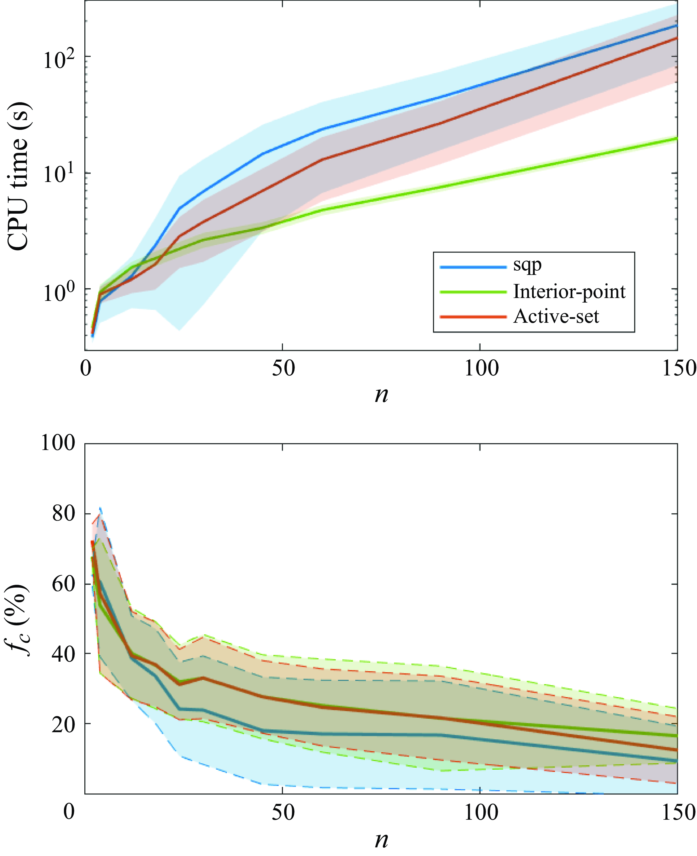
Figure 1. Computation time for calculating the maximal growth rate (a) and the relative frequency of solutions achieving the actual maximum (b) as functions of the dynamical system’s degrees of freedom. The shaded areas represent the standard deviation from the mean values.
The optimisation process was conducted for each dynamical model using 20 randomly generated transformation matrices, across a spectrum of relatively high perturbation levels $\gamma = { 0.1, 0.2, 0.5, 1, 2, 5, 10}$
. For each model, 100 randomly generated seed points – unitary
$\gamma = { 0.1, 0.2, 0.5, 1, 2, 5, 10}$
. For each model, 100 randomly generated seed points – unitary $\tilde {\boldsymbol{r}}$
state vectors – were created. From each seed point, optimisation was executed using three distinct algorithms. The global maximum for a given transformation matrix at a specified perturbation level was determined as the maximum across all optimisation techniques and seed points. The methods were compared based on the convergence rate, defined as the proportion of solutions that converged to the global maximum from differently initialised optimisations.
$\tilde {\boldsymbol{r}}$
state vectors – were created. From each seed point, optimisation was executed using three distinct algorithms. The global maximum for a given transformation matrix at a specified perturbation level was determined as the maximum across all optimisation techniques and seed points. The methods were compared based on the convergence rate, defined as the proportion of solutions that converged to the global maximum from differently initialised optimisations.
The convergence rate as a function of the number of degrees of freedom is depicted in figure 1(b), with the thick curve representing the mean value and the dashed line and shadow indicating the standard deviation of the convergence rate across various perturbation levels and transformation matrices. For systems with few degrees of freedom, the convergence rate was approximately 70 %, decreasing to 20 % as $n$
increases. For small systems (
$n$
increases. For small systems ( $n\lt 20$
), no significant difference was observed among the optimisation algorithms; however, for larger systems (
$n\lt 20$
), no significant difference was observed among the optimisation algorithms; however, for larger systems ( $n\gt 100$
), the interior-point algorithm clearly outperformed the others. Its mean convergence rate was higher, and its standard deviation was smaller. Although not visualised here, the convergence rate as a function of perturbation level was evaluated. For SQP and active set methods, the convergence rate decreased with increasing perturbation level, whereas for the interior-point algorithm, it remained nearly constant. Based on the convergence rate, the interior-point algorithm is superior, especially for large dynamical systems.
$n\gt 100$
), the interior-point algorithm clearly outperformed the others. Its mean convergence rate was higher, and its standard deviation was smaller. Although not visualised here, the convergence rate as a function of perturbation level was evaluated. For SQP and active set methods, the convergence rate decreased with increasing perturbation level, whereas for the interior-point algorithm, it remained nearly constant. Based on the convergence rate, the interior-point algorithm is superior, especially for large dynamical systems.
Computational time comparison, shown in figure 1(a), reveals that, for smaller systems ( $n\lt 12$
), the SQP method is the fastest. There exists a narrow range (
$n\lt 12$
), the SQP method is the fastest. There exists a narrow range ( $12\lt n\lt 20$
) where the active set method is optimal. For larger systems, the interior-point method is significantly faster than the other two methods, primarily because it utilises the analytical Hessian matrix, unlike the other methods.
$12\lt n\lt 20$
) where the active set method is optimal. For larger systems, the interior-point method is significantly faster than the other two methods, primarily because it utilises the analytical Hessian matrix, unlike the other methods.
In summary, the SQP method is recommended for small systems, while the interior-point method is better suited for larger ones. To determine the maximum growth rate for a given transformation matrix and perturbation level, optimisation is repeated from random initial points until at least five solutions converge to the same maximum value, reducing the risk of converging to a local maximum.
Since finding the global maximum is critical, the interior-point method’s convergence rate was analysed for dynamical models with up to 330 degrees of freedom. At this scale, the convergence rate drops to 5.81%. Assuming a sufficiently large sample, this rate can approximate the probability of locating the global maximum with a random initial guess. With 231 random initial guesses, the probability of missing the global maximum decreases to 1 in $10^6$
, making failures highly unlikely. The applied rule requiring at least five consistent results often necessitates even more initial guesses.
$10^6$
, making failures highly unlikely. The applied rule requiring at least five consistent results often necessitates even more initial guesses.
2.2.3. Calculation of the critical perturbation level
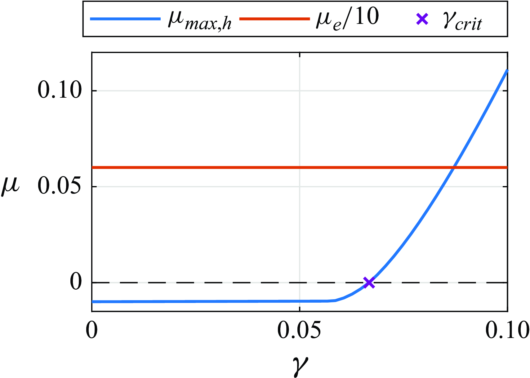
Figure 2. The maximal growth rate of the generalised kinetic energy ( $\mu _{{max}, h}$
) as the function perturbation magnitude
$\mu _{{max}, h}$
) as the function perturbation magnitude $\gamma$
in the case of the optimally transformed TTRD’ model at
$\gamma$
in the case of the optimally transformed TTRD’ model at $\textit{Re} = 5$
. The red curve represents the one tenth of the growth rate of the original kinetic energy (
$\textit{Re} = 5$
. The red curve represents the one tenth of the growth rate of the original kinetic energy ( $\mu _e = 0.6$
), which is independent of the perturbation level.
$\mu _e = 0.6$
), which is independent of the perturbation level.
As the $\mu _{{max},h}$
function is created by a proper optimisation procedure, the next step is to determine the largest possible critical perturbation level below which this growth is negative
$\mu _{{max},h}$
function is created by a proper optimisation procedure, the next step is to determine the largest possible critical perturbation level below which this growth is negative
 \begin{equation} \mu _{{max},h} (\textbf {S},\gamma _{{crit}}) = 0. \end{equation}
The corresponding unitary state vector, defined by
 \begin{equation} \mu _{{max},h} (\textbf {S},\gamma _{{crit}}) = \mu _h(\tilde {\boldsymbol{r}}_{{crit}}, \textbf {S},\gamma _{{crit}}), \end{equation}
can be utilised to obtain the critical state: $\boldsymbol{r}_{{crit}} = \gamma _{{crit}} \tilde {\boldsymbol{r}}_{{crit}}$
.
$\boldsymbol{r}_{{crit}} = \gamma _{{crit}} \tilde {\boldsymbol{r}}_{{crit}}$
.
For illustration, $\mu _{{max},h}$
is plotted in figure 2 for one particular problem. At low
$\mu _{{max},h}$
is plotted in figure 2 for one particular problem. At low $\gamma$
values, the linear part of the dynamical system dominates, where the maximum growth rate is almost constant and equal to the Rayleigh quotient of the
$\gamma$
values, the linear part of the dynamical system dominates, where the maximum growth rate is almost constant and equal to the Rayleigh quotient of the $\tilde {A}_{ij}+\tilde {A}_{ji}$
matrix, see equation (2.25). For higher
$\tilde {A}_{ij}+\tilde {A}_{ji}$
matrix, see equation (2.25). For higher $\gamma$
values, the nonlinearity of the system influences the maximal growth, which tends towards a straight line. The slope of this line corresponds to the maximum of
$\gamma$
values, the nonlinearity of the system influences the maximal growth, which tends towards a straight line. The slope of this line corresponds to the maximum of $\lbrace 2\, \, \tilde {Q}_{ijk}\,\tilde {r}_i\, \tilde {r}_j\,\tilde {r}_k\rbrace$
among possible
$\lbrace 2\, \, \tilde {Q}_{ijk}\,\tilde {r}_i\, \tilde {r}_j\,\tilde {r}_k\rbrace$
among possible $\tilde {r}_i$
states. Figure 2 illustrates the maximal growth rate of the original kinetic energy, highlighting that the laminar state is unstable according to the regular energy method. Moreover, it demonstrates that the original kinetic energy remains constant and is unaffected by the perturbation amplitude.
$\tilde {r}_i$
states. Figure 2 illustrates the maximal growth rate of the original kinetic energy, highlighting that the laminar state is unstable according to the regular energy method. Moreover, it demonstrates that the original kinetic energy remains constant and is unaffected by the perturbation amplitude.
Determining the critical perturbation level is relatively simpler compared with the other parts of the method. It involves finding the roots of equation (2.26). The gradient of this expression can be derived easily as
 \begin{equation} \frac {\partial \mu _{{max},h}}{\partial \gamma } = 2\, \tilde {Q}_{ijk}\,\tilde {r}_{{max},i}\, \tilde {r}_{{max},j}\,\tilde {r}_{{max},k} \end{equation}
where $\tilde {\boldsymbol{r}}_{{max}}$
is the vector that maximises the growth rate at a given perturbation level. By leveraging the analytical gradient, the Newton method, renowned for its second-order convergence rate, is utilised effectively. Typically, after a few iterations (5–6), the solution’s residual falls below the tolerated error threshold of
$\tilde {\boldsymbol{r}}_{{max}}$
is the vector that maximises the growth rate at a given perturbation level. By leveraging the analytical gradient, the Newton method, renowned for its second-order convergence rate, is utilised effectively. Typically, after a few iterations (5–6), the solution’s residual falls below the tolerated error threshold of $10^{-10}$
.
$10^{-10}$
.
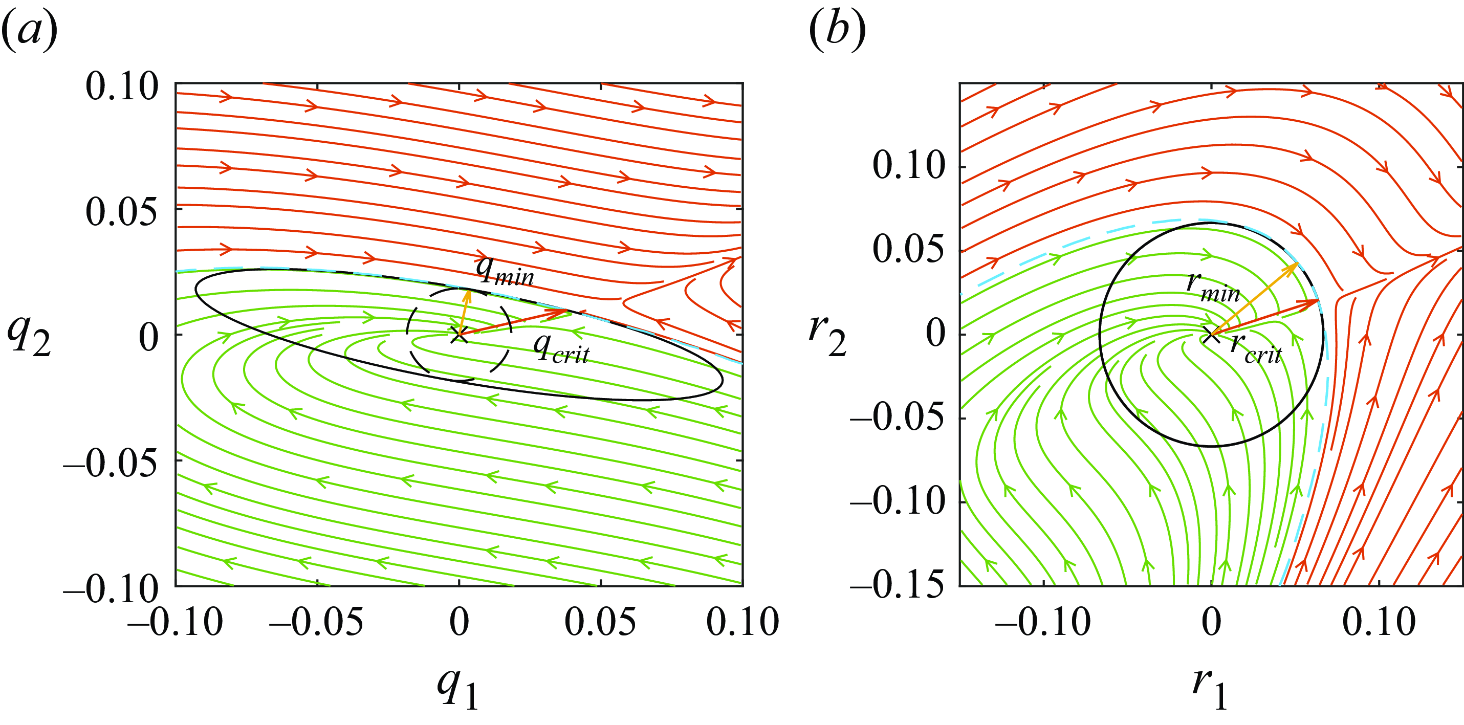
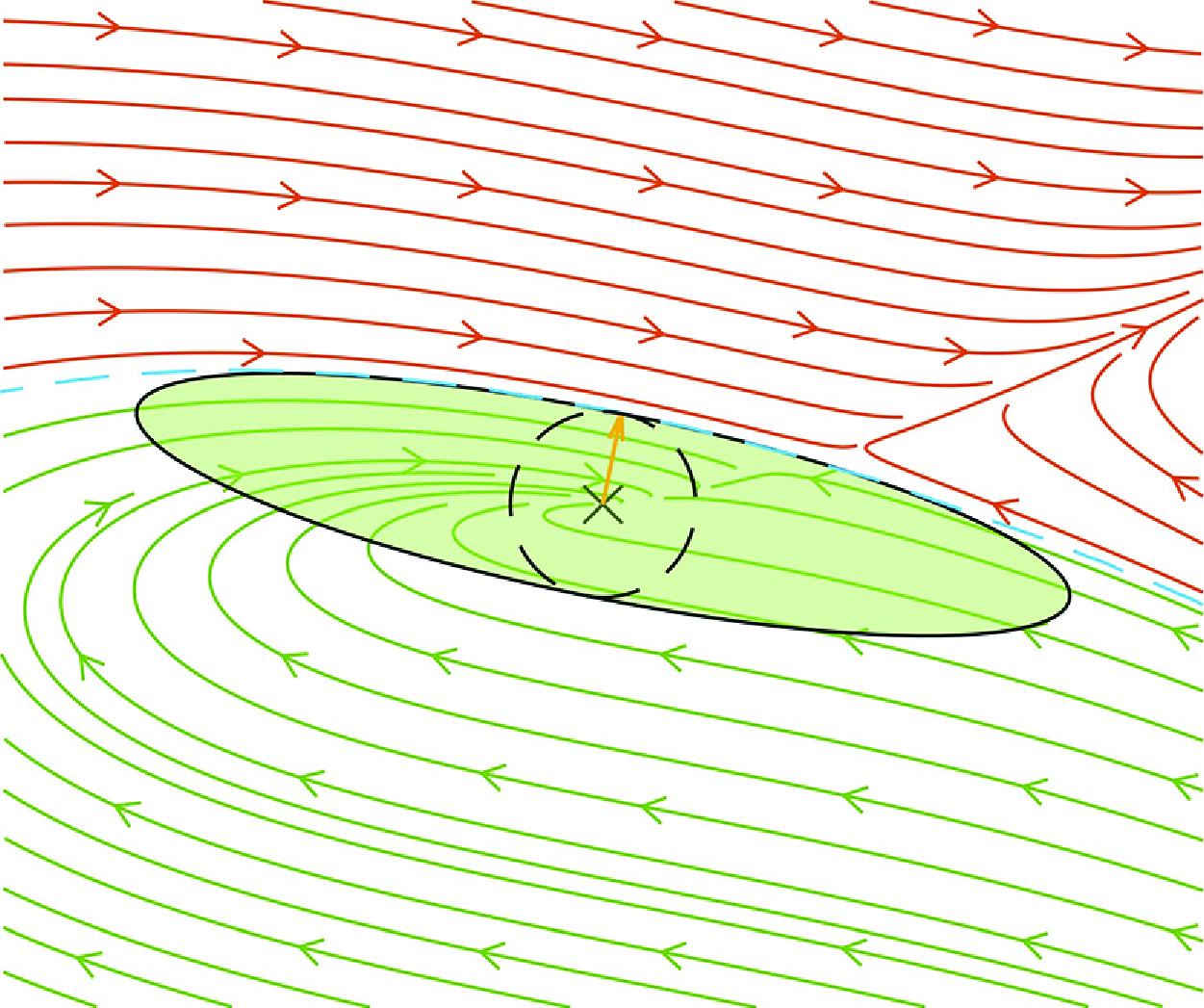
Figure 3. The phase space trajectories of the TTRD’ model at $\textit{Re} = 5$
are shown for the original state variables (a) and for the optimally transformed variables (b). Green trajectories converge towards the origin, while red trajectories tend to another equilibrium point, which is not shown. The black curve represents the provable boundary of the ROA utilising the optimal
$\textit{Re} = 5$
are shown for the original state variables (a) and for the optimally transformed variables (b). Green trajectories converge towards the origin, while red trajectories tend to another equilibrium point, which is not shown. The black curve represents the provable boundary of the ROA utilising the optimal $h$
function. The dashed, blue curve shows the boundary of the true ROA. The red vector is the critical perturbation (2.26), where the growth rate of the generalised kinetic energy was zero at the critical perturbation level (2.27). The yellow vector illustrates the smallest perturbation (2.30) in the original state space (a) whose length is equal to the critical perturbation in the optimally transformed state space (b).
$h$
function. The dashed, blue curve shows the boundary of the true ROA. The red vector is the critical perturbation (2.26), where the growth rate of the generalised kinetic energy was zero at the critical perturbation level (2.27). The yellow vector illustrates the smallest perturbation (2.30) in the original state space (a) whose length is equal to the critical perturbation in the optimally transformed state space (b).
The investigated region can be envisioned as a multidimensional hypersphere in the $\boldsymbol{r}$
state space around the origin. The radius of this sphere is
$\boldsymbol{r}$
state space around the origin. The radius of this sphere is $\gamma$
. If the radius is smaller than a critical value
$\gamma$
. If the radius is smaller than a critical value $\gamma _{{crit}}$
, then
$\gamma _{{crit}}$
, then $\mu _h\lt 0$
, indicating that the generalised kinetic energy (
$\mu _h\lt 0$
, indicating that the generalised kinetic energy ( $h$
) is decreasing, and the trajectories move inward, ultimately converging to the origin. At the critical radius, a trajectory becomes tangential to the sphere and may not reach the origin. The hypersphere with radius
$h$
) is decreasing, and the trajectories move inward, ultimately converging to the origin. At the critical radius, a trajectory becomes tangential to the sphere and may not reach the origin. The hypersphere with radius $\gamma _{{crit}}$
represents the boundary of the provable ROA. However, states outside this sphere can belong to the basin of attraction of either the origin or another attractor. In the case of the two-dimensional problem, the hyperspherical ROA reduces to a circle and is illustrated in figure 3(b) in the case of an optimal transformation matrix and
$\gamma _{{crit}}$
represents the boundary of the provable ROA. However, states outside this sphere can belong to the basin of attraction of either the origin or another attractor. In the case of the two-dimensional problem, the hyperspherical ROA reduces to a circle and is illustrated in figure 3(b) in the case of an optimal transformation matrix and $h$
function.
$h$
function.
It is more interpretable to transform the ROA back to the original state space. The linear transformation (scaling and rotating) of the hypersphere results in a hyperellipsoid in the original state space $\boldsymbol{q}$
. This hyperellipsoid defines the boundary of the provable ROA of the origin. A standard quantity describing ROA is its smallest radius,
$\boldsymbol{q}$
. This hyperellipsoid defines the boundary of the provable ROA of the origin. A standard quantity describing ROA is its smallest radius, $\sqrt {e_{{min}}}$
.
$\sqrt {e_{{min}}}$
.
The value $e_{{min}}$
can be calculated using equations (2.2) and (2.21) as follows:
$e_{{min}}$
can be calculated using equations (2.2) and (2.21) as follows:
 \begin{equation} e_{{min}}(\textbf {S}) = \gamma _{{crit}}^2 (\textbf {S}) \min _{\tilde {\boldsymbol{r}}} \lbrace \tilde {\boldsymbol{r}}^T \textbf {S}^T \textbf {S} \tilde {\boldsymbol{r}} \rbrace . \end{equation}
The argument of the minimum function is the Rayleigh quotient of $\textbf {S}^T \textbf {S}$
, and the minimum value corresponds to the smallest eigenvalue of
$\textbf {S}^T \textbf {S}$
, and the minimum value corresponds to the smallest eigenvalue of $\textbf {S}^T \textbf {S}$
, since
$\textbf {S}^T \textbf {S}$
, since $\textbf {S}^T \textbf {S}$
is a symmetric matrix
$\textbf {S}^T \textbf {S}$
is a symmetric matrix
 \begin{equation} e_{{min}}(\textbf {S}) = \gamma _{{crit}}^2 (\textbf {S}) \;\lambda _{{min}} \big ( {\textbf {S}^T \textbf {S}}\big ) . \end{equation}
The corresponding unitary eigenvector $\tilde {\boldsymbol{r}}_{{min}}$
can be utilised to get the two locations
$\tilde {\boldsymbol{r}}_{{min}}$
can be utilised to get the two locations $\boldsymbol{q}_{{min}} = \pm \gamma _{{crit}}\,\textbf {S}\, \tilde {\boldsymbol{r}}_{{min}} = \pm \textbf {S}\, \boldsymbol{r}_{{min}}$
, where the inner hypersphere touches the hyperellipsoid, as illustrated in figure 3(a). This inner hypersphere is a subset of the provable ROA, where
$\boldsymbol{q}_{{min}} = \pm \gamma _{{crit}}\,\textbf {S}\, \tilde {\boldsymbol{r}}_{{min}} = \pm \textbf {S}\, \boldsymbol{r}_{{min}}$
, where the inner hypersphere touches the hyperellipsoid, as illustrated in figure 3(a). This inner hypersphere is a subset of the provable ROA, where $e\lt e_{{min}}$
.
$e\lt e_{{min}}$
.
The value of $e_{{min}}$
depends on the definition of
$e_{{min}}$
depends on the definition of $h$
through the transformation matrix
$h$
through the transformation matrix $\textbf {S}$
. The aim of the method is to maximise this minimum energy,
$\textbf {S}$
. The aim of the method is to maximise this minimum energy, $e_{{min}}(\textbf {S})$
over all matrices,
$e_{{min}}(\textbf {S})$
over all matrices, $\textbf {S}$
. The possible methods for maximisation will be discussed in § 2.3. It is important to note that the value of
$\textbf {S}$
. The possible methods for maximisation will be discussed in § 2.3. It is important to note that the value of $\gamma$
is only meaningful for a specific transformation or generalised kinetic energy. Comparisons of
$\gamma$
is only meaningful for a specific transformation or generalised kinetic energy. Comparisons of $\gamma$
or
$\gamma$
or $\gamma _{{crit}}$
between different
$\gamma _{{crit}}$
between different $\textbf {S}$
matrices or
$\textbf {S}$
matrices or $h$
functions are not valid.
$h$
functions are not valid.
It should also be mentioned that although the kinetic energy ( $e$
) can grow significantly inside the provable ROA region – a phenomenon usually called the non-modal growth – stability is guaranteed there due to the exponential decay of
$e$
) can grow significantly inside the provable ROA region – a phenomenon usually called the non-modal growth – stability is guaranteed there due to the exponential decay of $h$
there.
$h$
there.
2.3. Optimising the generalised kinetic energy
The last key question is how to determine the optimal $h$
function, represented by the transformation matrix
$h$
function, represented by the transformation matrix $\textbf {S}_{{opt}}$
, to maximise the size of the provable ROA,
$\textbf {S}_{{opt}}$
, to maximise the size of the provable ROA, $e_{{min}}$
. First, a method utilising the singular value decomposition (SVD) of the eigenvectors is presented. This method cannot provide the largest
$e_{{min}}$
. First, a method utilising the singular value decomposition (SVD) of the eigenvectors is presented. This method cannot provide the largest $e_{{min}}$
, but it is extremely fast compared with other methods. As a second approach, all the elements of the transformation matrix are treated as decision variables, leading to a significantly larger ROA at the cost of higher computational need.
$e_{{min}}$
, but it is extremely fast compared with other methods. As a second approach, all the elements of the transformation matrix are treated as decision variables, leading to a significantly larger ROA at the cost of higher computational need.
2.3.1. The GKE-SV method utilising the singular value decomposition of the eigenvector matrix
A plausible starting point is to use the eigenvectors of $\textbf {A}$
,
$\textbf {A}$
, $\boldsymbol{\Psi }_c$
, as the transformation matrix, since it diagonalises the
$\boldsymbol{\Psi }_c$
, as the transformation matrix, since it diagonalises the $\textbf {A}$
matrix. This transformation redefines the state variables as coefficients of the eigenmodes, addressing non-normality by making
$\textbf {A}$
matrix. This transformation redefines the state variables as coefficients of the eigenmodes, addressing non-normality by making $\tilde {\textbf {A}}$
diagonal and its eigenvectors orthogonal. Consequently, the GKE, expressed as the sum of squared eigenmode coefficients, ensures stability at infinitesimally low perturbation levels, as noted by Olivier Dauchot & Paul Manneville (Reference Dauchot and Manneville1997).
$\tilde {\textbf {A}}$
diagonal and its eigenvectors orthogonal. Consequently, the GKE, expressed as the sum of squared eigenmode coefficients, ensures stability at infinitesimally low perturbation levels, as noted by Olivier Dauchot & Paul Manneville (Reference Dauchot and Manneville1997).
Diagonalising $\textbf {A}$
with
$\textbf {A}$
with $\boldsymbol{\Psi }_c$
results in the maximum linear growth rate of
$\boldsymbol{\Psi }_c$
results in the maximum linear growth rate of
 \begin{equation} \mu _{h,\mathit{lin,max}} (\boldsymbol{\Psi }_c) = \lambda _{{max}}\big (\tilde {\textbf {A}} +\tilde {\textbf {A}}^T\big ) = 2 {\textit{Re}} \big (\lambda _{{max}} (\textbf {A})\big ), \end{equation}
which must be negative if the equilibrium point is linearly stable and there exists a certain provable ROA. However, it will be shown that $\boldsymbol{\Psi }_c$
used to define
$\boldsymbol{\Psi }_c$
used to define $h$
is not optimal, but systematic modifications can yield an improved transformation matrix and
$h$
is not optimal, but systematic modifications can yield an improved transformation matrix and $h$
.
$h$
.
As a first step, the eigenvector matrix is transformed into a real-valued matrix, denoted as $\boldsymbol{\Psi }$
. This involves reinterpreting all eigenvector pairs associated with the same complex-conjugate eigenvalue pairs, alternately focusing on the real and imaginary components, and subsequently normalising these to unit vectors. Although this new transformation matrix does not diagonalise the
$\boldsymbol{\Psi }$
. This involves reinterpreting all eigenvector pairs associated with the same complex-conjugate eigenvalue pairs, alternately focusing on the real and imaginary components, and subsequently normalising these to unit vectors. Although this new transformation matrix does not diagonalise the $\textbf {A}$
matrix, the formulation of generalised energy remains analogous and equation (2.31) still holds.
$\textbf {A}$
matrix, the formulation of generalised energy remains analogous and equation (2.31) still holds.
Next, the SVD of $\boldsymbol{\Psi }$
matrix is performed
$\boldsymbol{\Psi }$
matrix is performed
 \begin{equation} \boldsymbol{\Psi } = \textbf {U}_\psi \,\textbf {S}_\psi \,\textbf {V}_\psi . \end{equation}
It can be demonstrated that $\textbf {V}_\psi$
does not affect the definition of
$\textbf {V}_\psi$
does not affect the definition of $h$
in equation (2.15) and
$h$
in equation (2.15) and $\textbf {V}_\psi$
can therefore be omitted.
$\textbf {V}_\psi$
can therefore be omitted.
For simplicity, the singular values can be normalised by their maximum without sacrificing generality. Furthermore, let the singular values be denoted by $s_i$
, where
$s_i$
, where $s_1$
is the largest and
$s_1$
is the largest and $s_n$
is the smallest. Due to normalisation
$s_n$
is the smallest. Due to normalisation $s_1 = 1$
and
$s_1 = 1$
and $0\lt s_i\leqslant 1$
. It is well known that, as the Reynolds number increases, the non-normality of A or the condition number of the eigenvector matrix increases. Therefore, the smallest singular value of
$0\lt s_i\leqslant 1$
. It is well known that, as the Reynolds number increases, the non-normality of A or the condition number of the eigenvector matrix increases. Therefore, the smallest singular value of $\boldsymbol{\Psi }$
,
$\boldsymbol{\Psi }$
, $s_n$
, tends toward zero, leading to two significant issues. One problem is that a decreasing
$s_n$
, tends toward zero, leading to two significant issues. One problem is that a decreasing $s_n$
makes the eigenvector matrix ill conditioned and difficult to invert accurately. Additionally, this choice likely reduces the size of ROA,
$s_n$
makes the eigenvector matrix ill conditioned and difficult to invert accurately. Additionally, this choice likely reduces the size of ROA, $e_{{min}}$
, since
$e_{{min}}$
, since
 \begin{equation} e_{{min}}\,\propto \, \lambda _{{min}}\big (\textbf {S}^T\textbf {S}\big ) = s_n^2 ,\end{equation}
according to equation (2.30). Visually, utilising $\boldsymbol{\Psi }$
as the transformation matrix results in an attraction region shaped like a narrow superellipsoid with its smallest axis shrinking to zero. In this context, the concept of ‘exotic’ energy as defined by Olivier Dauchot & Paul Manneville (Reference Dauchot and Manneville1997), while effective for two-dimensional systems at lower Reynolds numbers, is presumably inefficient for larger systems or those at higher Reynolds numbers, where the ratio of the smallest and largest singular values of
$\boldsymbol{\Psi }$
as the transformation matrix results in an attraction region shaped like a narrow superellipsoid with its smallest axis shrinking to zero. In this context, the concept of ‘exotic’ energy as defined by Olivier Dauchot & Paul Manneville (Reference Dauchot and Manneville1997), while effective for two-dimensional systems at lower Reynolds numbers, is presumably inefficient for larger systems or those at higher Reynolds numbers, where the ratio of the smallest and largest singular values of $\boldsymbol{\Psi }$
becomes large.
$\boldsymbol{\Psi }$
becomes large.
A straightforward solution to the problem is proposed by modifying the transformation matrix as
 \begin{equation} \textbf {S} = \textbf {U}_\psi \,\tilde {\textbf {S}}_\psi, \end{equation}
where $\textbf {U}_\psi$
comes from the SVD decomposition of
$\textbf {U}_\psi$
comes from the SVD decomposition of $\boldsymbol{\Psi }$
and
$\boldsymbol{\Psi }$
and $\tilde {\textbf {S}}$
is the modified matrix of the singular values (
$\tilde {\textbf {S}}$
is the modified matrix of the singular values ( $\textbf {S}_\psi$
), for which the singular values smaller than a certain threshold,
$\textbf {S}_\psi$
), for which the singular values smaller than a certain threshold, $s_{{min}}$
, are simply set to
$s_{{min}}$
, are simply set to $s_{{min}}$
 \begin{equation} \tilde {s}_i = \begin{cases} s_i \,\,\; &\mathrm{if} \, s_i\gt s_{{min}}, \\ s_{{min}} \, &\mathrm{if} \, s_i\leqslant s_{{min}} .\end{cases} \end{equation}
The threshold parameter, $s_{{min}}$
, can be set between
$s_{{min}}$
, can be set between $s_n$
and 1. If
$s_n$
and 1. If $s_{{min}} = s_n$
, the transformation matrix is equivalent to the eigenvector matrix in terms of the
$s_{{min}} = s_n$
, the transformation matrix is equivalent to the eigenvector matrix in terms of the $h$
definition. Conversely, if
$h$
definition. Conversely, if $s_{{min}}$
is set to 1, the transformation has no effect, making the GKE equivalent to
$s_{{min}}$
is set to 1, the transformation has no effect, making the GKE equivalent to $e$
. In this case, if
$e$
. In this case, if $\textit{Re} \gt \textit{Re}_E$
, no provable ROA exists according to
$\textit{Re} \gt \textit{Re}_E$
, no provable ROA exists according to $h$
.
$h$
.
By varying $s_{{min}}$
, between the two extrema,
$s_{{min}}$
, between the two extrema, $\mu _{h,{lin, max}}$
increases continuously and changes sign. This behaviour is illustrated in figure 4, which shows the maximal growth rate of the linearised system rate after transformation as a function of
$\mu _{h,{lin, max}}$
increases continuously and changes sign. This behaviour is illustrated in figure 4, which shows the maximal growth rate of the linearised system rate after transformation as a function of $s_{{min}}$
for the
$s_{{min}}$
for the $n=210$
PFM at
$n=210$
PFM at $\textit{Re} = 2000$
. Interestingly, for various systems,
$\textit{Re} = 2000$
. Interestingly, for various systems, $s_{{min}}$
can be increased by orders of magnitude above the smallest original singular values without significantly affecting
$s_{{min}}$
can be increased by orders of magnitude above the smallest original singular values without significantly affecting $\mu _{h,{lin,max}}$
. In the presented case,
$\mu _{h,{lin,max}}$
. In the presented case, $s_{{min}}$
is increased by two orders of magnitude without altering
$s_{{min}}$
is increased by two orders of magnitude without altering $\mu _{h,{lin,max}}$
. This demonstrates that the non-normality of
$\mu _{h,{lin,max}}$
. This demonstrates that the non-normality of $\textbf {A}$
can be effectively managed without relying on an ill-conditioned transformation matrix. Moreover, increasing
$\textbf {A}$
can be effectively managed without relying on an ill-conditioned transformation matrix. Moreover, increasing $s_{{min}}$
significantly enlarges the provable ROA, as
$s_{{min}}$
significantly enlarges the provable ROA, as $\sqrt {e_{{min}}}$
is proportional to the smallest singular value of the transformation matrix.
$\sqrt {e_{{min}}}$
is proportional to the smallest singular value of the transformation matrix.
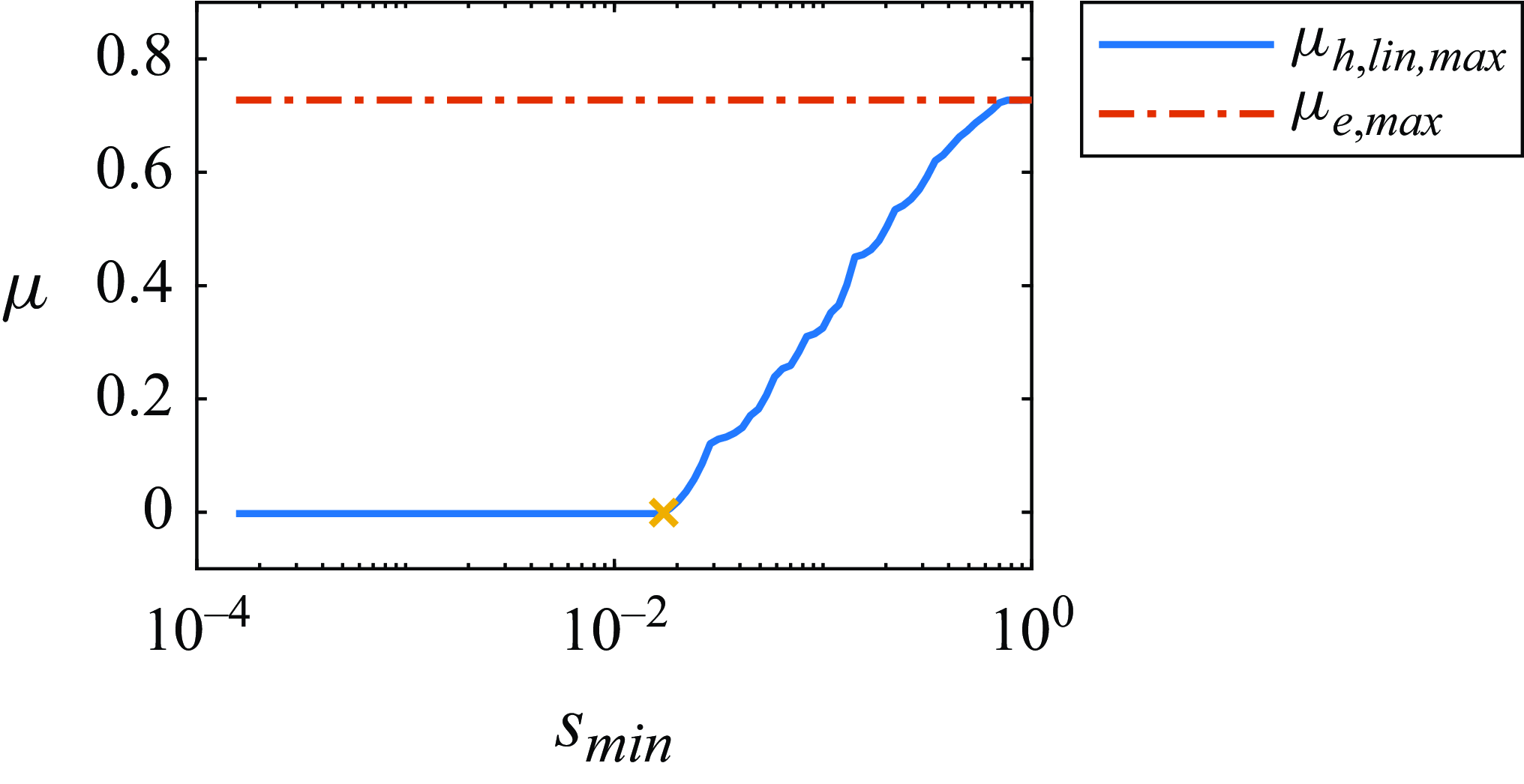
Figure 4. The maximal growth rate of the GKE ( $\mu _{h, {lin,max}}$
) for the linearised system, plotted against the smallest singular value of the modified eigenvector matrix at
$\mu _{h, {lin,max}}$
) for the linearised system, plotted against the smallest singular value of the modified eigenvector matrix at $\textit{Re} = 2000$
. The system in question is the 210-dimensional PFM. The red curve depicts the maximal growth rate of the original kinetic energy, while the yellow cross marks the critical
$\textit{Re} = 2000$
. The system in question is the 210-dimensional PFM. The red curve depicts the maximal growth rate of the original kinetic energy, while the yellow cross marks the critical $s_{{min}}$
value at which the growth rate becomes zero.
$s_{{min}}$
value at which the growth rate becomes zero.
During the optimisation of the transformation matrix, the optimal $s_{{min}}$
is determined using a bisection algorithm. The algorithm increases
$s_{{min}}$
is determined using a bisection algorithm. The algorithm increases $s_n$
with a relative accuracy of
$s_n$
with a relative accuracy of $10^{-3}$
until
$10^{-3}$
until $\mu _{h,{lin,max}}$
no longer exceeds a relative change of
$\mu _{h,{lin,max}}$
no longer exceeds a relative change of $10^{-5}$
from its minimum possible value.
$10^{-5}$
from its minimum possible value.
The optimisation of $\textbf {S}$
such a way offers both benefits and limitations due to its disregard for nonlinear terms. This exclusion streamlines the optimisation, significantly speeding up the process as it necessitates only the eigenvalue analysis of relatively small matrices. After optimising the transformation matrix, a solitary evaluation is sufficient for computing the ROA. However, this method may not achieve optimality, given that it neglects the impact of nonlinear terms during the optimisation of the transformation matrix. This approach has been named the ‘GKE-SV’ algorithm in the context of this study.
$\textbf {S}$
such a way offers both benefits and limitations due to its disregard for nonlinear terms. This exclusion streamlines the optimisation, significantly speeding up the process as it necessitates only the eigenvalue analysis of relatively small matrices. After optimising the transformation matrix, a solitary evaluation is sufficient for computing the ROA. However, this method may not achieve optimality, given that it neglects the impact of nonlinear terms during the optimisation of the transformation matrix. This approach has been named the ‘GKE-SV’ algorithm in the context of this study.
2.3.2. The GKE-G method – general optimisation of the transformation matrix
An alternative approach involves optimising the elements of the transformation matrix as decision variables to maximise the size of the provable ROA, $e_{{min}}$
value. Given that only the definition of
$e_{{min}}$
value. Given that only the definition of $h$
(
$h$
( $\textbf {P}$
in equation (2.15)) affects the stability analysis, we can assume, without loss of generality, that
$\textbf {P}$
in equation (2.15)) affects the stability analysis, we can assume, without loss of generality, that $\textbf {S}$
is an upper triangular matrix. This assumption reduces the number of unknowns from
$\textbf {S}$
is an upper triangular matrix. This assumption reduces the number of unknowns from $n^2$
to
$n^2$
to $(n^2+n)/2$
. As the degrees of freedom expand, the number of decision variables increases quadratically, necessitating gradient-based optimisation. The derivation of the gradient is elaborated in Appendix A.2.
$(n^2+n)/2$
. As the degrees of freedom expand, the number of decision variables increases quadratically, necessitating gradient-based optimisation. The derivation of the gradient is elaborated in Appendix A.2.
This approach to optimising the transformation matrix is comprehensive, allowing for the identification of the optimum among all possible quadratic Lyapunov functions. Despite this advantage, the method requires multiple evaluations of the ROA, making it computationally intensive. Even with the utilisation of gradients with respect to decision variables to expedite the process, the computational demands remain significant. To manage the complexity and the high number of unknowns efficiently, the interior-point algorithm is employed in this study.
The general optimisation procedure for $\textbf {S}$
unfolds as follows:
$\textbf {S}$
unfolds as follows:
-
(i) Solve (2.26) to determine $\gamma _{{crit}}$
.
$\gamma _{{crit}}$
. -
(ii) Calculate
$e_{{min}}$
through (2.30). -
(iii) Update
$\textbf {S}$
through the interior-point algorithm, guided by the gradient (A9), and iteratively repeat the first two steps until
$e_{{min}}$
(2.30) reaches its maximum value.


This methodical enhancement of $\textbf {S}$
ensures that the optimisation steadily moves towards a maximum of
$\textbf {S}$
ensures that the optimisation steadily moves towards a maximum of $e_{{min}}$
, which can of course be only local rather than global. In the paper, this optimisation procedure of the transformation matrix is referred to as the ‘GKE-G’ algorithm.
$e_{{min}}$
, which can of course be only local rather than global. In the paper, this optimisation procedure of the transformation matrix is referred to as the ‘GKE-G’ algorithm.
2.4. Comparison of the generalised kinetic energy method and sum-of-squares programs
This section introduces a comparison between the proposed procedure for constructing Lyapunov functions and the current state-of-the-art methodologies, particularly those employing SOS programs. A brief description of the applied SOS methods is provided in Appendices A.2.1 and A.2.2.
The first SOS program, SOS1 (Jarvis-Wloszek Reference Jarvis-Wloszek2003; Tan & Packard Reference Tan and Packard2008; Topcu et al. Reference Topcu, Packard and Seiler2008; Khodadadi et al. Reference Khodadadi, Samadi and Khaloozadeh2014; Kalur et al. Reference Kalur, Seiler and Hemati2021), consists of three SOS constraints, one ensures the positive definiteness of the Lyapunov function, the second maximises the size of the ROA while the third mandates that the Lyapunov function decreases along the solution trajectories. The maximal ROA can be obtained by an iterative maximisation of the parameters of the constraints.
The second SOS program, SOS2 (Liu & Gayme Reference Liu and Gayme2020), is similar to the SOS1 program but the second constraint is replaced by an eigenvalue problem, significantly reducing the size of the problem and the necessary number of iterations. Therefore, SOS2 is usually faster but less accurate compared with the SOS1 method.
There is a convex formulation, SOS3, for inner approximating a basin of attraction introduced by Henrion & Korda (Reference Henrion and Korda2014) which avoids the necessary iteration steps of the SOS1 and SOS2 programs. However, in SOS3, time appears as an explicit variable in the polynomials, unlike in SOS1 and SOS2. Additionally, SOS3 consist of four SOS constraints, resulting in significantly larger optimisation problem. Furthermore, it requires the explicit specification of a time horizon and a target domain. These parameters play a critical role in shaping the results. This formulation is excluded from the comparison.
The two SOS algorithms and the two GKE algorithms were evaluated against each other using simple models, focusing on computational time and the size of the ROA as key metrics. For the conversion of SOS programs into a semi-definite program (SDP), two tools, SOSTOOLS (Papachristodoulou et al. Reference Papachristodoulou, Anderson, Valmorbida, Prajna, Seiler and Parrilo2013) and Yalmip (Löfberg Reference Löfberg2004), were employed. However, no significant difference in computational time was observed between them. Consequently, the results presented here utilise the conversion code provided by SOSTOOLS, with the SDP problems solved using MOSEK.
The ROA was calculated for five dynamical systems: TTRD’, W95A, W95B, BT and PFM $_{n=12}$
. These systems have degrees of freedom (
$_{n=12}$
. These systems have degrees of freedom ( $n$
) of 2, 4, 4, 4 and 12 respectively. Here, PFM
$n$
) of 2, 4, 4, 4 and 12 respectively. Here, PFM $_{n=12}$
denotes the truncated Galerkin model of Poiseuille flow, while the other models are low-order representations of subcritical transition. These calculations were performed on a computer equipped with an Intel i7-7700 processor running at 3.6 GHz and 32 GB of memory with a speed of 2400 MHz.
$_{n=12}$
denotes the truncated Galerkin model of Poiseuille flow, while the other models are low-order representations of subcritical transition. These calculations were performed on a computer equipped with an Intel i7-7700 processor running at 3.6 GHz and 32 GB of memory with a speed of 2400 MHz.
The comparative analysis in figure 5 illustrates the performance differences between the GKE and SOS algorithms in determining the ROA for dynamical systems. The GKE-G algorithm identified a ROA radius identical to that of the SOS1 method for low-dimensional models ( $n \leqslant 4$
) and slightly smaller for the
$n \leqslant 4$
) and slightly smaller for the $n = 12$
model, but required more time to do so. The small difference is attributed to the optimisation of the
$n = 12$
model, but required more time to do so. The small difference is attributed to the optimisation of the $h$
function in the GKE-G method. When the optimal
$h$
function in the GKE-G method. When the optimal $h$
definition obtained by the SOS1 algorithm was used to calculate the provable ROA using the GKE-G method, the radius matched that of the SOS1 method. The SOS2 algorithm yielded a slightly smaller ROA, whereas the GKE-SV algorithm predicted significantly smaller regions but demanded substantially less computational resources.
$h$
definition obtained by the SOS1 algorithm was used to calculate the provable ROA using the GKE-G method, the radius matched that of the SOS1 method. The SOS2 algorithm yielded a slightly smaller ROA, whereas the GKE-SV algorithm predicted significantly smaller regions but demanded substantially less computational resources.
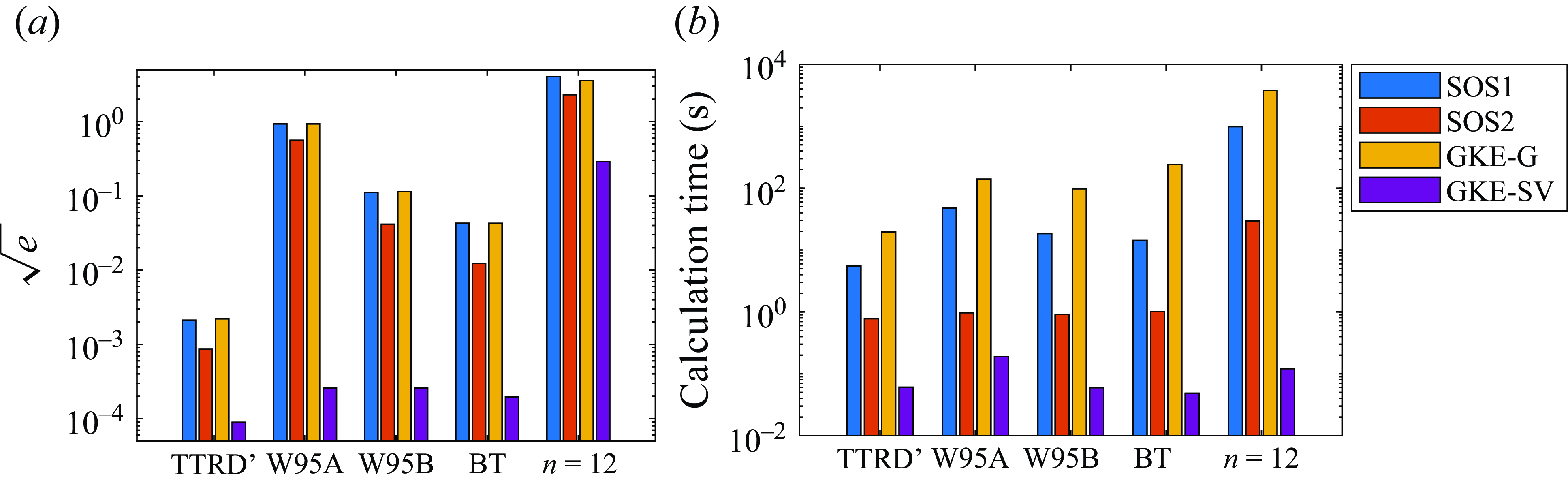
Figure 5. Threshold amplitude (a) across five dynamical systems (TTRD’, W95A, W95B, BT, PFM $_{n=12}$
) at a Reynolds number of
$_{n=12}$
) at a Reynolds number of $\textit{Re} = 5\textit{Re}_E$
, as determined by four distinct methods, alongside the computational time (b).
$\textit{Re} = 5\textit{Re}_E$
, as determined by four distinct methods, alongside the computational time (b).
For smaller systems, the SOS1 algorithm is recommended due to its precision. The increased computational demand typically does not pose a significant concern for these cases. However, it has been discovered that the SOS1 method becomes impractical for systems with more than 15 degrees of freedom, as the resultant SDP becomes too large for the optimisation program, MOSEK, to solve. Similar limitations were observed with the SOS2 algorithm when the degrees of freedom exceeded 21.
A core issue identified is that, even when restricting the analysis to quadratic Lyapunov functions, the left-hand side of equations (A18–A19) in SOS1 and (A22) in SOS2 manifest as fourth-order polynomials. To ascertain their positive definiteness, the necessary number of monomials is proportional to $n^2$
, implying that the optimisation matrix size – containing the decision variables – scales roughly with
$n^2$
, implying that the optimisation matrix size – containing the decision variables – scales roughly with $n^4$
. Consequently, the number of decision variables surges as the degrees of freedom (
$n^4$
. Consequently, the number of decision variables surges as the degrees of freedom ( $n$
) increase. The SOS2 algorithm accommodates slightly larger systems due to involving only one fourth-order polynomial, in contrast to the two present in SOS1.
$n$
) increase. The SOS2 algorithm accommodates slightly larger systems due to involving only one fourth-order polynomial, in contrast to the two present in SOS1.
Conversely, GKE methods exhibit scalability to systems an order of magnitude larger, as will be demonstrated. Notably, the GKE-G method provides an approximation of the ROA comparable in accuracy to the widely utilised SOS1 method, offering a viable alternative for larger system analysis. The GKE method exemplifies a less conservative approach with better scalability.
3. Application
3.1. Trefethen’s and Waleffe’s models
Well-known low-order dynamical systems that mimic the subcritical transition of shear flows are investigated in this study. Specifically, the two-dimensional TTRD’ model of Baggett & Trefethen (Reference Baggett and Trefethen1997) and the four-dimensional W95 model of Waleffe (Reference Waleffe1995) are examined. In these models, the linearised part (A) is non-normal, and the condition number of its eigenvector matrix grows with increasing Reynolds number. Meanwhile, the nonlinear part does not affect the growth rate of kinetic energy, as the corresponding matrix remains asymmetric.
The TTRD’ model is represented by the following equation:
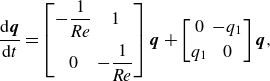 \begin{align} \frac {\mathrm{d}\boldsymbol{q}}{\mathrm{d}t}= \begin{bmatrix} -\dfrac {1}{\textit{Re}} & 1 \\[8pt] 0 &-\dfrac {1}{\textit{Re}} \\ \end{bmatrix} \boldsymbol{q}+ \begin{bmatrix} 0 & -q_1 \\[3pt] q_1 &0 \end{bmatrix}\boldsymbol{q}, \end{align}
therefore the non-zero elements of $Q_{ijk}$
are
$Q_{ijk}$
are
 \begin{align}& Q_{1\,1\,2} = -1 , \\[-12pt] \nonumber \end{align}
 \begin{align}&\,\, Q_{2\,1\,1} = 1. \end{align}
The optimal $h$
functions and the corresponding transformation matrices for TTRD’, that maximise
$h$
functions and the corresponding transformation matrices for TTRD’, that maximise $e_{{min}}$
, are calculated at the Reynolds number between 5 and 100 with the step size 2.5 by the proposed GKE-G method. The result is visualised in figure 3 at
$e_{{min}}$
, are calculated at the Reynolds number between 5 and 100 with the step size 2.5 by the proposed GKE-G method. The result is visualised in figure 3 at $\textit{Re}=5$
, where green trajectories converge to the origin and red trajectories to another state. These trajectories are shown in the original variables (figure 3
a) and the transformed variables (figure 3
b). The calculated ROA appears as an ellipse in the original state space, precisely touching the boundary of the true ROA.
$\textit{Re}=5$
, where green trajectories converge to the origin and red trajectories to another state. These trajectories are shown in the original variables (figure 3
a) and the transformed variables (figure 3
b). The calculated ROA appears as an ellipse in the original state space, precisely touching the boundary of the true ROA.
Next, the calculated threshold amplitude as the function of Reynolds number are plotted in figure 6 and compared with the findings of Liu & Gayme (Reference Liu and Gayme2020). The cited authors used the quadratic constraint method, which has been proven to be computationally efficient. They treated the nonlinear term as a forcing with an approximated upper bound.
The calculated threshold amplitude ( $\sqrt {e_{{min}}}$
) decays as a function of the Reynolds number following a power law. The exponents are nearly identical: −3.005 in this study and −3.07 in the work of Liu & Gayme (Reference Liu and Gayme2020). However, the method presented here predicts a ROA with a radius roughly three times larger, indicating a energy level approximately one magnitude higher. This substantial difference arises from their approximation of the nonlinear term, while GKE-G calculation takes into account the exact terms, providing a more precise representation of the system’s behaviour, similarly to SOS methods.
$\sqrt {e_{{min}}}$
) decays as a function of the Reynolds number following a power law. The exponents are nearly identical: −3.005 in this study and −3.07 in the work of Liu & Gayme (Reference Liu and Gayme2020). However, the method presented here predicts a ROA with a radius roughly three times larger, indicating a energy level approximately one magnitude higher. This substantial difference arises from their approximation of the nonlinear term, while GKE-G calculation takes into account the exact terms, providing a more precise representation of the system’s behaviour, similarly to SOS methods.
In the next step, the accuracy of the ROA is investigated by solving the ordinary differential equation initialised close to the outside of the calculated ROA. The solutions are initialised from slightly increased threshold state vectors $\boldsymbol{q}_{0} = c_{u} \boldsymbol{q}_{{min}}$
approximating the minimal seed states and computed using the Matlab ode45 Runge–Kutta method.
$\boldsymbol{q}_{0} = c_{u} \boldsymbol{q}_{{min}}$
approximating the minimal seed states and computed using the Matlab ode45 Runge–Kutta method.
The average value of $c_{u}$
for such solutions is found to be 1.02, indicating that the proposed method is highly accurate for this small model. The energy level of these approximated minimal seeds are shown in figure 6 but they are almost on the curve representing the radius of ROA.
$c_{u}$
for such solutions is found to be 1.02, indicating that the proposed method is highly accurate for this small model. The energy level of these approximated minimal seeds are shown in figure 6 but they are almost on the curve representing the radius of ROA.
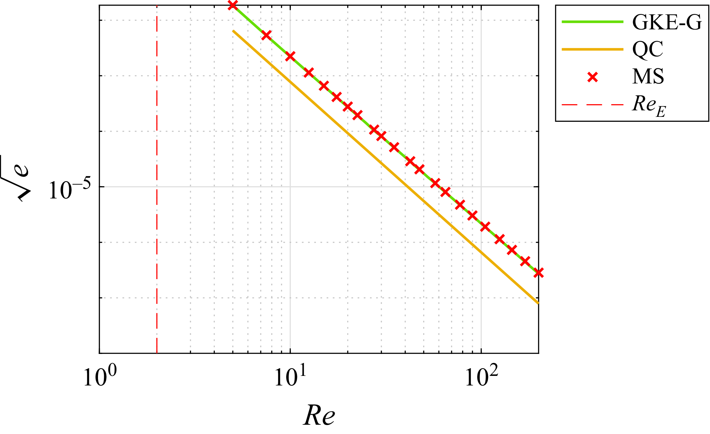
Figure 6. The size of ROA as the function of Reynolds number in the case of TTRD’ model. The fitted curve from Liu & Gayme (Reference Liu and Gayme2020) using the QC method $(0.912\,\textit{Re}^{-3.07})$
is shown alongside. The best-fitting curve of GKE-G results is
$(0.912\,\textit{Re}^{-3.07})$
is shown alongside. The best-fitting curve of GKE-G results is $\sqrt {e_{{min}}}\approx 2.228 \,\textit{Re}^{-3.005}$
. The red crosses represent the energy of the approximated minimal seeds. The vertical red line signifies the unconditional stability limit
$\sqrt {e_{{min}}}\approx 2.228 \,\textit{Re}^{-3.005}$
. The red crosses represent the energy of the approximated minimal seeds. The vertical red line signifies the unconditional stability limit $\textit{Re}_E = 2$
.
$\textit{Re}_E = 2$
.
In the next step, the GKE-G method is applied to the low-order model of subcritical transition proposed by Waleffe (Reference Waleffe1995). The dynamical system is represented as follows:
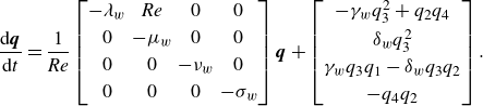 \begin{equation} \frac {\mathrm{d}\boldsymbol{q}}{\mathrm{d}t}=\frac {1}{\textit{Re}} \begin{bmatrix} -\lambda _w & \textit{Re} & 0 & 0\\[3pt] 0 &-\mu _w & 0 & 0\\[3pt] 0 & 0 &-\nu _w & 0 \\[3pt] 0 & 0 & 0 &-\sigma _w \\ \end{bmatrix} \boldsymbol{q}+ \begin{bmatrix} -\gamma _w q_3^2 + q_2 q_4 \\[3pt] \delta _w q_3^2 \\[3pt] \gamma _w q_3 q_1-\delta _w q_3 q_2 \\[3pt] -q_4 q_2 \\ \end{bmatrix}. \end{equation}
The parameters $\lambda _w, \mu _w, \nu _w, \sigma _w$
represent the decay rates due to viscosity, while
$\lambda _w, \mu _w, \nu _w, \sigma _w$
represent the decay rates due to viscosity, while $\gamma _w, \delta _w$
describe the nonlinear interaction between rolls (
$\gamma _w, \delta _w$
describe the nonlinear interaction between rolls ( $q_2$
) and streaks (
$q_2$
) and streaks ( $q_1$
).
$q_1$
).
In this study, three different parameter sets are investigated. The first set is characterised by $\lambda _w = \mu _w= \sigma _w = 10,\, \nu _w = 15,\, \delta _w = 1,\, \gamma _w = 0.1$
, denoted as the W95A model (Waleffe Reference Waleffe1995). The parameters of the second set remain the same except
$\lambda _w = \mu _w= \sigma _w = 10,\, \nu _w = 15,\, \delta _w = 1,\, \gamma _w = 0.1$
, denoted as the W95A model (Waleffe Reference Waleffe1995). The parameters of the second set remain the same except $\gamma _w = 0.5$
, and this configuration is denoted as W95B. In the last case, all parameters are set to 1,
$\gamma _w = 0.5$
, and this configuration is denoted as W95B. In the last case, all parameters are set to 1, $\lambda _w = \mu _w= \nu _w =\sigma _w =\delta _w = 1$
, and this configuration is denoted as the BT model (Baggett & Trefethen Reference Baggett and Trefethen1997). It is important to note that these parameter sets significantly influence the system dynamics (Baggett & Trefethen Reference Baggett and Trefethen1997; Kalur et al. Reference Kalur, Seiler and Hemati2021).
$\lambda _w = \mu _w= \nu _w =\sigma _w =\delta _w = 1$
, and this configuration is denoted as the BT model (Baggett & Trefethen Reference Baggett and Trefethen1997). It is important to note that these parameter sets significantly influence the system dynamics (Baggett & Trefethen Reference Baggett and Trefethen1997; Kalur et al. Reference Kalur, Seiler and Hemati2021).
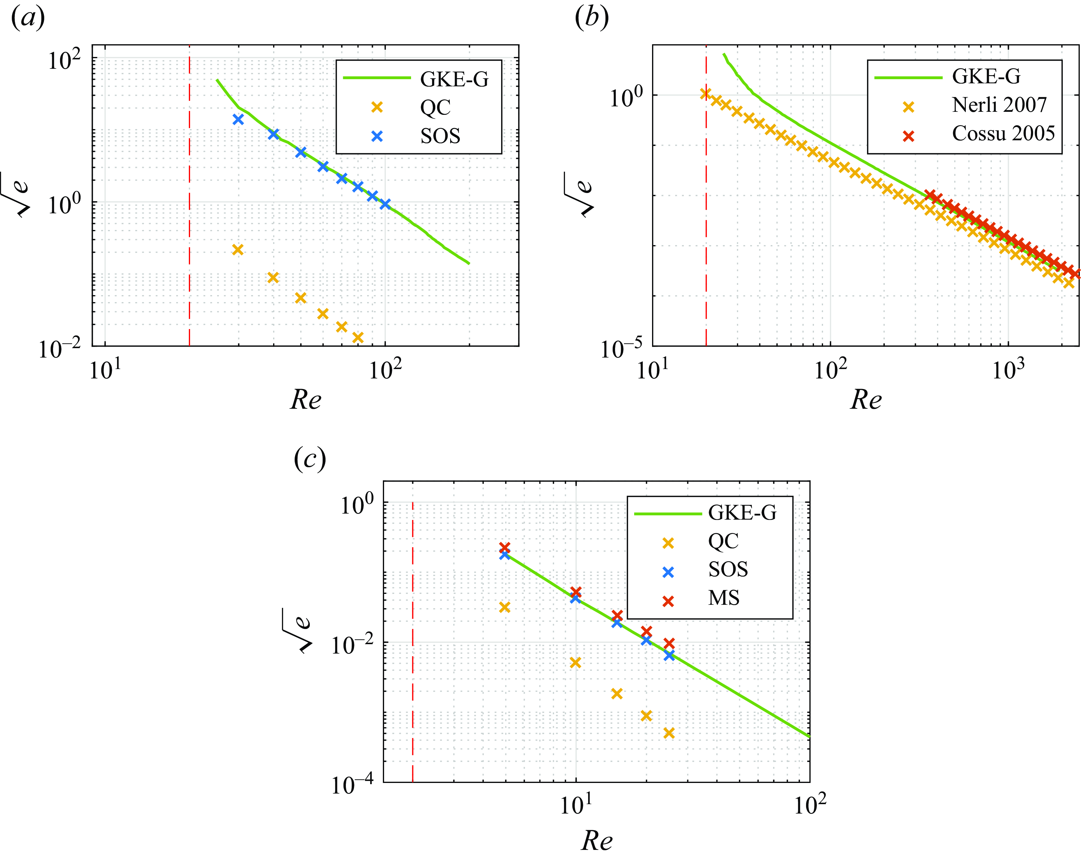
Figure 7. The size of the ROA as the function of the Reynolds number in the case of the W95A model (a), W95B model (b) and BT model (c), computed using the GKE-G method. The QC, SOS, MS curves represent the results of Kalur et al. (Reference Kalur, Seiler and Hemati2021) and MS refers to minimal seeds obtained via direct-adjoint looping. For the W95B model, the minimal seed energy is taken from Cossu (Reference Cossu2005). The red, vertical dashed line indicates the unconditional stability limit, $\textit{Re}_E$
. The best-fitting curves of
$\textit{Re}_E$
. The best-fitting curves of $\sqrt {e_{{min}}}$
:
$\sqrt {e_{{min}}}$
: $\sqrt {e_{{min}}} \approx 176479 \,\textit{Re}^{-2.65089}$
for W95A;
$\sqrt {e_{{min}}} \approx 176479 \,\textit{Re}^{-2.65089}$
for W95A; $\sqrt {e_{{min}}}\approx 1964.3 \,\textit{Re}^{-2.08506}$
for W95B;
$\sqrt {e_{{min}}}\approx 1964.3 \,\textit{Re}^{-2.08506}$
for W95B; $\sqrt {e_{{min}}}\approx 4.1952 \,\textit{Re}^{-1.98875}$
for BT model.
$\sqrt {e_{{min}}}\approx 4.1952 \,\textit{Re}^{-1.98875}$
for BT model.
The optimised transformation matrices are calculated for the W95A, W95B and BT models over different ranges of Reynolds numbers: 25–200 for the W95A model, 25–2000 for the W95B model and 5–100 for the BT model by the GKE-G method. For the W95A and BT models, the step size was set to 2.5, while for the W95B model, a logarithmic spacing was applied over 150 steps. Figure 7 shows the largest inner radius of the ROA for the three models.
The proposed GKE-G method is compared with other stability calculation methods. For the W95A and BT models, it yields nearly identical allowable perturbation levels as the SOS1 method employed by Kalur et al. (Reference Kalur, Seiler and Hemati2021), indicating that these are the largest provable ROA utilising quadratic Lyapunov functions.
Kalur et al. (Reference Kalur, Seiler and Hemati2021) also applied the QC method to the same W95A and BT models, predicting significantly smaller regions due to the approximation of nonlinear terms using bounds, despite its lower computational cost. A comparative analysis of the QC method across different model dimensions (TTRD’, W95A, BT) reveals a decreasing accuracy with increasing model complexity.
For the W95B model, the calculated allowable perturbation levels are compared with the results of Nerli et al. (Reference Nerli, Camarri and Salvetti2007). The presented GKE-G implementation slightly outperforms the GKE method of Nerli et al. (Reference Nerli, Camarri and Salvetti2007) due to a more general energy function form. (It is mentioned that Nerli et al. (Reference Nerli, Camarri and Salvetti2007) defined the kinetic energy with a multiplier of 1/2 which was compensated by a factor of $1/\sqrt {2}$
on the plots here.) Additionally, the calculated allowable threshold energy levels by the GKE-G method are close to the energy levels of minimal seeds calculated by Cossu (Reference Cossu2005). Since the minimal seeds represent states with the lowest kinetic energy converging to another attractor, the close agreement between stability threshold energy and minimal seed energy indicates accurate approximation of the stability region boundary. Similar observations hold for the BT model, where minimal seeds (MS) are calculated by Kalur et al. (Reference Kalur, Seiler and Hemati2021) using direct-adjoint looping.
$1/\sqrt {2}$
on the plots here.) Additionally, the calculated allowable threshold energy levels by the GKE-G method are close to the energy levels of minimal seeds calculated by Cossu (Reference Cossu2005). Since the minimal seeds represent states with the lowest kinetic energy converging to another attractor, the close agreement between stability threshold energy and minimal seed energy indicates accurate approximation of the stability region boundary. Similar observations hold for the BT model, where minimal seeds (MS) are calculated by Kalur et al. (Reference Kalur, Seiler and Hemati2021) using direct-adjoint looping.
In contrast, the results for the W95A model show different behaviour. Solutions initialised outside the predicted ROA tend to a laminar state, as also observed by Kalur et al. (Reference Kalur, Seiler and Hemati2021). This suggests that the true ROA is significantly larger than the predicted and might be better captured using higher-order Lyapunov functions.
In summary, the GKE-G method accurately predicts perturbation thresholds for the two-dimensional TTRD’ model and the four-dimensional BT and W95B models. However, for the W95A model, the method proves overly conservative, necessitating higher-order Lyapunov functions to capture a larger ROA.
3.2. Poiseuille flow models
To construct a reasonably accurate yet comparatively low-dimensional model of the two-dimensional Poiseuille flow we will use Galerkin projection on the basis of eigenfunctions of the Stokes operator. The construction method is described in Appendix B.
The chosen dimension of the domain is $L_x=2 \pi$
to ensure that the base wavenumber (
$L_x=2 \pi$
to ensure that the base wavenumber ( $\alpha _0=2 \pi /L_x=1$
) aligns closely with the critical value identified through linear stability analysis, which is
$\alpha _0=2 \pi /L_x=1$
) aligns closely with the critical value identified through linear stability analysis, which is $\alpha = 1.02$
according to Orszag (Reference Orszag1971).
$\alpha = 1.02$
according to Orszag (Reference Orszag1971).
To determine an appropriate number of modes for the analysis, an initial assessment was conducted on the reduced-order model’s linear stability, followed by an examination of the original energy stability.
Initially, the linear stability limit ( $\textit{Re}_{{L}}$
) is determined by identifying when the first eigenvalue of the linear part (
$\textit{Re}_{{L}}$
) is determined by identifying when the first eigenvalue of the linear part ( $\textbf {A}$
) turns positive. The influence of the number of modes at a particular wavenumber pairs,
$\textbf {A}$
) turns positive. The influence of the number of modes at a particular wavenumber pairs, $N_y$
within the range of 10–50 is depicted in table 1. It becomes apparent that, for fewer than 30 modes, the outcome of the linear stability analysis is markedly sensitive to the mode count, a phenomenon attributable to the high susceptibility of the non-normal linear operator to numerical inaccuracies, as highlighted by Trefethen & Embree (Reference Trefethen and Embree2005).
$N_y$
within the range of 10–50 is depicted in table 1. It becomes apparent that, for fewer than 30 modes, the outcome of the linear stability analysis is markedly sensitive to the mode count, a phenomenon attributable to the high susceptibility of the non-normal linear operator to numerical inaccuracies, as highlighted by Trefethen & Embree (Reference Trefethen and Embree2005).
Table 1. The critical Reynolds numbers, as determined through linear stability analysis ( $\textit{Re}_L$
) and energy stability analysis (
$\textit{Re}_L$
) and energy stability analysis ( $\textit{Re}_E$
), for the two-dimensional PFM with domain size
$\textit{Re}_E$
), for the two-dimensional PFM with domain size $L_x=2 \pi$
and
$L_x=2 \pi$
and $N_z=0$
. Values selected for further analysis in this study are highlighted in bold.
$N_z=0$
. Values selected for further analysis in this study are highlighted in bold.
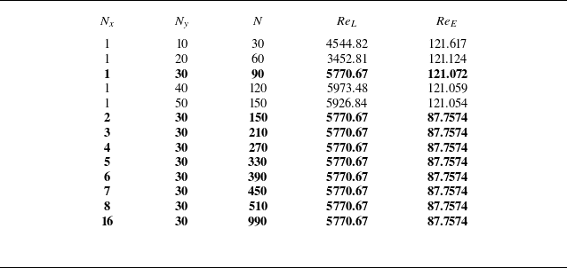
Concurrently, the energy stability limit ( $\textit{Re}_{{E}}$
) exhibits less sensitivity to the choice of modes
$\textit{Re}_{{E}}$
) exhibits less sensitivity to the choice of modes $N_y$
and numerical errors. Notably, as the number of streamwise modes
$N_y$
and numerical errors. Notably, as the number of streamwise modes $N_x$
is increased from 1 to 2, a significant shift in the limit from 121 to 87 is observed. However, further increments in the number of streamwise modes do not influence the outcome. This indicates that the critical perturbation for classical energy analysis corresponds to a wavenumber of
$N_x$
is increased from 1 to 2, a significant shift in the limit from 121 to 87 is observed. However, further increments in the number of streamwise modes do not influence the outcome. This indicates that the critical perturbation for classical energy analysis corresponds to a wavenumber of $2\alpha _0 = 2$
, whereas, according to linear stability analysis, the streamwise wavenumber of the critical perturbation is
$2\alpha _0 = 2$
, whereas, according to linear stability analysis, the streamwise wavenumber of the critical perturbation is $\alpha _0 = 1$
for this configuration.
$\alpha _0 = 1$
for this configuration.
These two limits serve as pivotal benchmarks for the model and can be calculated with relative ease. Below the energy stability limit, the flow is deemed unconditionally stable, implying an infinite radius for the ROA. Conversely, beyond the linear stability limit, the flow becomes unconditionally unstable, reducing the radius of the ROA to zero. Within the bounds of these two limits, the proposed method offers a viable approach to ascertain the conditional stability threshold.
For the models under consideration, the threshold amplitudes are computed with $N_y=30$
. This provides a balance between the error margin of the linear stability limit and the number of modes.
$N_y=30$
. This provides a balance between the error margin of the linear stability limit and the number of modes.
The evaluation of the models spans Reynolds numbers from 250 to 2000, in increments of 250. Given the complexity associated with a high number of degrees of freedom, which reaches 90 for the smallest model studied, the SOS methods are deemed impractical for estimating the threshold amplitude. Instead, the GKE-G method is utilised for models up to $N_x = 5$
, where the results indicate convergence. For demonstration purposes, the GKE-SV method is applied to the largest systems up to
$N_x = 5$
, where the results indicate convergence. For demonstration purposes, the GKE-SV method is applied to the largest systems up to $N_x = 16$
and
$N_x = 16$
and $n=990$
.
$n=990$
.
The figure 8(a) presents the allowable perturbation amplitude for various models at $\textit{Re} = 500$
. It depicts the square root of the ratio of allowable perturbation kinetic energy to the base flow kinetic energy (
$\textit{Re} = 500$
. It depicts the square root of the ratio of allowable perturbation kinetic energy to the base flow kinetic energy ( $E$
), essentially showcasing the proportionality between the magnitude of perturbation velocity and the base flow velocity. This metric is henceforth referred to as the threshold amplitude ratio.
$E$
), essentially showcasing the proportionality between the magnitude of perturbation velocity and the base flow velocity. This metric is henceforth referred to as the threshold amplitude ratio.
In the application of the GKE-G method, notable variations in results persist until the number of degrees of freedom reaches 210 ( $N_x=3$
), beyond which increases to 270 (
$N_x=3$
), beyond which increases to 270 ( $N_x=4$
) or 330 (
$N_x=4$
) or 330 ( $N_x=5$
) result in only slight changes. It is important to note that the optimisation process of the transformation matrix does not utilise results from lower-order dynamical systems, rendering these results independently obtained. The convergence of the threshold amplitude ratio, therefore, suggests that the optimisation either identifies the global maximum of the allowable perturbation level or converges to a similar local maximum across various system sizes.
$N_x=5$
) result in only slight changes. It is important to note that the optimisation process of the transformation matrix does not utilise results from lower-order dynamical systems, rendering these results independently obtained. The convergence of the threshold amplitude ratio, therefore, suggests that the optimisation either identifies the global maximum of the allowable perturbation level or converges to a similar local maximum across various system sizes.
When the transformation matrix is optimised using the GKE-SV method, the predicted allowable perturbation level is lower, as anticipated. This reduction is due to the optimisation focusing solely on the singular values of the $\boldsymbol{\Psi }$
matrix and considering only the linear component of the dynamical system. However, these substantial simplifications in determining the optimal transformation matrix yield a threshold amplitude that is less than one magnitude smaller than that predicted by the GKE-G method. Conversely, the previously described QC method predicts significantly lower threshold amplitude levels, even for smaller dynamical systems.
$\boldsymbol{\Psi }$
matrix and considering only the linear component of the dynamical system. However, these substantial simplifications in determining the optimal transformation matrix yield a threshold amplitude that is less than one magnitude smaller than that predicted by the GKE-G method. Conversely, the previously described QC method predicts significantly lower threshold amplitude levels, even for smaller dynamical systems.
Figure 8(b) compares the computational times between the two optimisation approaches. The benefits of employing the GKE-SV method are evident; not only is the computational time orders of magnitude lower, but it also facilitates application to larger dynamical systems, underscoring its efficiency and scalability.
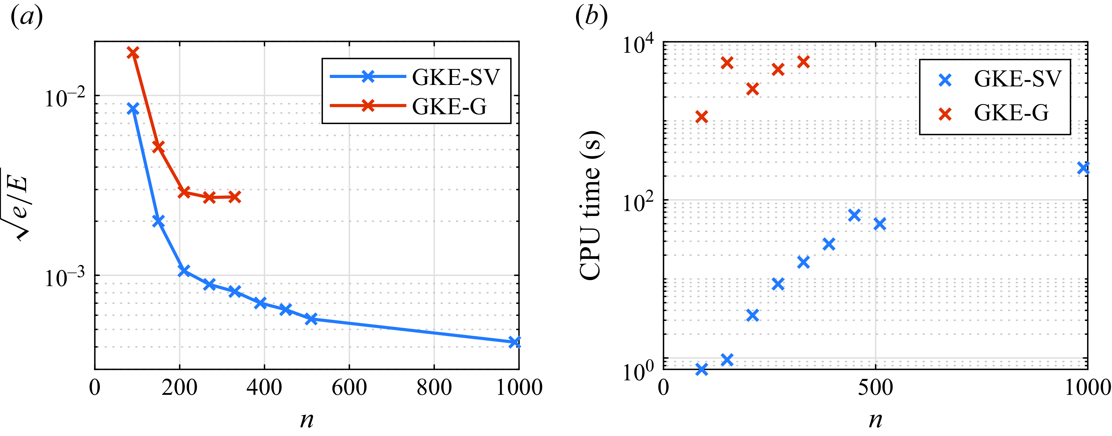
Figure 8. (a) The square root of the ratio of allowable perturbation kinetic energy to the base flow kinetic energy, plotted as a function of degrees of freedom for a two-dimensional Poiseuille flow at $\textit{Re} = 500$
. The periodic domain length is set to
$\textit{Re} = 500$
. The periodic domain length is set to $L_x = 2\pi$
. (b) The computational time required for the analysis.
$L_x = 2\pi$
. (b) The computational time required for the analysis.
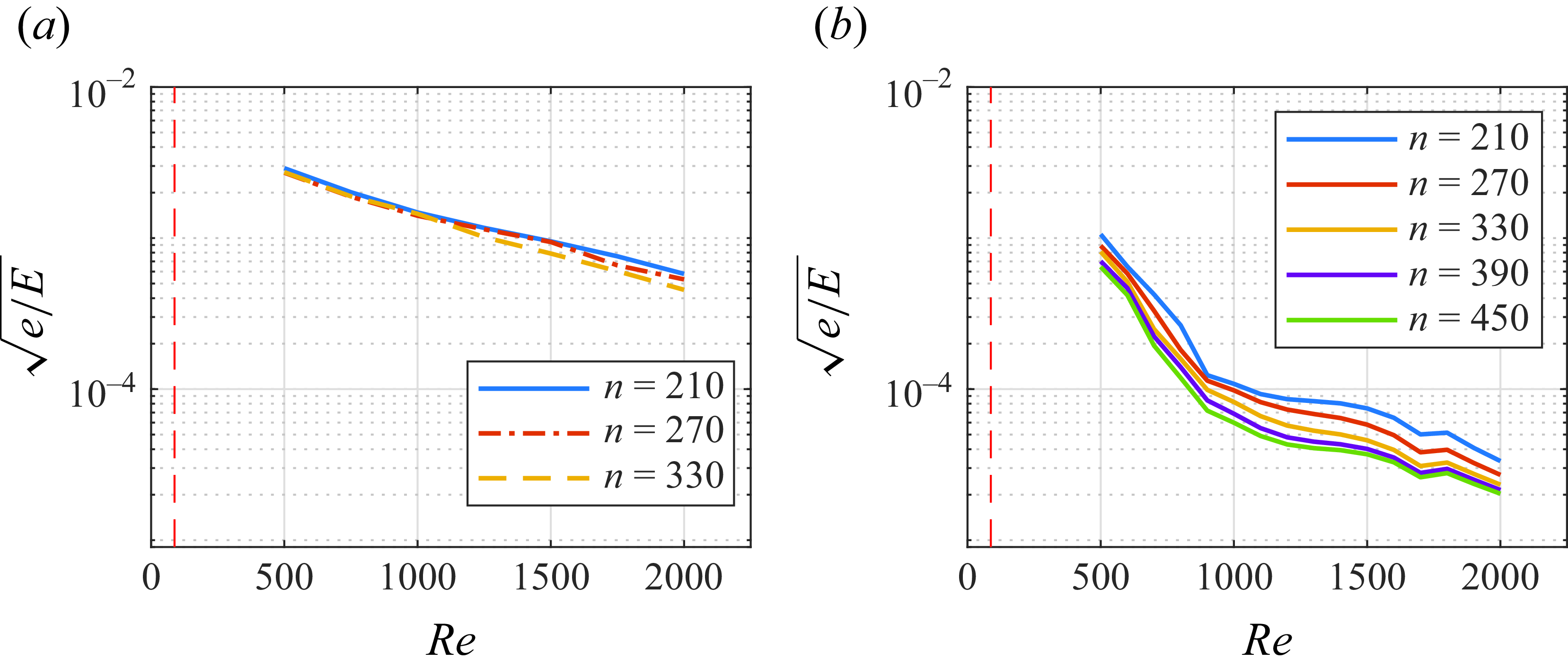
Figure 9. The square root of the ratio of allowable perturbation kinetic energy to the base flow kinetic energy plotted against the Reynolds number for various PFMs. The transformation matrix optimisation is carried out using (a) the GKE-G method and (b) the GKE-SV method.
Next, the threshold amplitude ratio as a function of Reynolds number is depicted in figure 9. When the transformation matrix is optimised using the GKE-G method for models with $n = 210, 270, 330$
, the resulting curves closely align with one another, with only minor deviations observed at higher Reynolds numbers. The figure plots the threshold amplitude ratio on a logarithmic y-axis against a linear x-axis. The nearly linear curves suggest a decay rate faster than a power law, consistent with the flow’s linear instability at a finite Reynolds number, where the threshold amplitude approaches zero.
$n = 210, 270, 330$
, the resulting curves closely align with one another, with only minor deviations observed at higher Reynolds numbers. The figure plots the threshold amplitude ratio on a logarithmic y-axis against a linear x-axis. The nearly linear curves suggest a decay rate faster than a power law, consistent with the flow’s linear instability at a finite Reynolds number, where the threshold amplitude approaches zero.
In figure 9(a), the threshold amplitudes obtained using the GKE-SV method are presented. The amplitude ratios are notably lower than those calculated via the GKE-G method, which can be attributed to the simpler optimisation process previously discussed. Additionally, fluctuations are observed around at $\textit{Re} = 1700$
, highlighting the sub-optimality of the GKE-SV method. These fluctuations result from the restrictions imposed on the transformation matrix, which vary with the Reynolds number but remain consistent across the models since they describe the same shear flow configuration. As the Reynolds number increases, the disparity between the results from the two methods widens, yet the difference remains under two magnitudes even at the highest Reynolds number evaluated.
$\textit{Re} = 1700$
, highlighting the sub-optimality of the GKE-SV method. These fluctuations result from the restrictions imposed on the transformation matrix, which vary with the Reynolds number but remain consistent across the models since they describe the same shear flow configuration. As the Reynolds number increases, the disparity between the results from the two methods widens, yet the difference remains under two magnitudes even at the highest Reynolds number evaluated.
The findings are juxtaposed with the minimal seed calculations conducted by Zhang & Tao (Reference Zhang and Tao2023), who determined that the laminar flow remains globally stable up to a Reynolds number of 2332.5. Zhang calculated the energy of the minimal seed at $\textit{Re}=2333$
to be approximately
$\textit{Re}=2333$
to be approximately $e_{\mathit{MS}} = 0.01$
. From this value, the estimated amplitude ratio of the minimal seed,
$e_{\mathit{MS}} = 0.01$
. From this value, the estimated amplitude ratio of the minimal seed, $\sqrt {e_{\mathit{MS}}/E}$
, is roughly 0.007. This represents the amplitude limit beyond which perturbations persist within the system. In our analysis utilising the 330-dimensional model with the GKE-G method, the threshold amplitude – up to which the laminar flow maintains stability – is approximately
$\sqrt {e_{\mathit{MS}}/E}$
, is roughly 0.007. This represents the amplitude limit beyond which perturbations persist within the system. In our analysis utilising the 330-dimensional model with the GKE-G method, the threshold amplitude – up to which the laminar flow maintains stability – is approximately $\sqrt {e_{{min}}/E}=0.00045$
at
$\sqrt {e_{{min}}/E}=0.00045$
at $\textit{Re}=2000$
. This value is only one magnitude smaller than the minimal seed estimation. However, it is important to note that their results were obtained in a significantly larger domain of
$\textit{Re}=2000$
. This value is only one magnitude smaller than the minimal seed estimation. However, it is important to note that their results were obtained in a significantly larger domain of $L_x=400$
, compared with the domain length of
$L_x=400$
, compared with the domain length of $L_x = 2\pi$
employed in our study.
$L_x = 2\pi$
employed in our study.
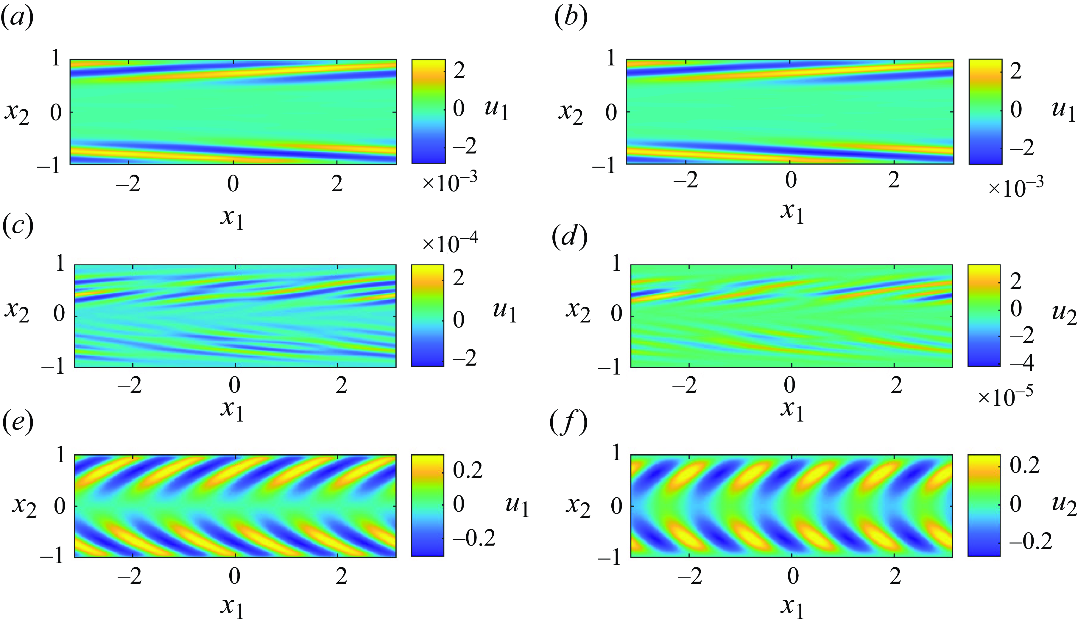
Figure 10. Perturbation field for the truncated PFM with $n=330$
at
$n=330$
at $\textit{Re}=1000$
. Panels (a) and (b) show the states with the smallest energy (
$\textit{Re}=1000$
. Panels (a) and (b) show the states with the smallest energy ( $e_{{min}}$
) on the boundary of provable ROA calculated using the GKE-G method. Panels (c) and (d) depict the same states using the GKE-SV method. Panels (e) and (f) present the perturbations with the highest growth rate according to the original energy method. The streamwise and wall-normal velocity components are shown in the left and right columns, respectively.
$e_{{min}}$
) on the boundary of provable ROA calculated using the GKE-G method. Panels (c) and (d) depict the same states using the GKE-SV method. Panels (e) and (f) present the perturbations with the highest growth rate according to the original energy method. The streamwise and wall-normal velocity components are shown in the left and right columns, respectively.
In figure 10, panels (a–d) present the perturbations with the smallest kinetic energy ( $e_{{min}}$
) at the boundary of the provable ROA for both the GKE-G and GKE-SV methods. In the case of the GKE-G method, these perturbations manifest as tilted periodic waves localised near the walls, resembling the minimal seed states described by Zhang & Tao (Reference Zhang and Tao2023). However, due to the significantly longer domain (100 units) used in their study, sometimes localised structures in the streamwise direction were observed, depending on the initial perturbation amplitude and Reynolds number. The shorter domain length (
$e_{{min}}$
) at the boundary of the provable ROA for both the GKE-G and GKE-SV methods. In the case of the GKE-G method, these perturbations manifest as tilted periodic waves localised near the walls, resembling the minimal seed states described by Zhang & Tao (Reference Zhang and Tao2023). However, due to the significantly longer domain (100 units) used in their study, sometimes localised structures in the streamwise direction were observed, depending on the initial perturbation amplitude and Reynolds number. The shorter domain length ( $2 \pi$
) in our study likely excludes the observation of such structures, resulting in fully periodic structures instead.
$2 \pi$
) in our study likely excludes the observation of such structures, resulting in fully periodic structures instead.
For the GKE-SV method, the perturbations appear as stripes localised between the wall and the domain’s centreline. These perturbations are less structured and exhibit asymmetry, likely due to the sub-optimal nature of the GKE-SV method.
For reference, panels (e–f) in figure 10, show the critical perturbation with the highest growth rate ( $\mu _e = 0.7712$
) according to the original energy method. These perturbations also appear as tilted periodic waves, as demonstrated by Farrell (Reference Farrell1988), but are less localised to the near-wall region and exhibit higher oscillations in the streamwise direction compared with the critical perturbations according to the GKE-G method.
$\mu _e = 0.7712$
) according to the original energy method. These perturbations also appear as tilted periodic waves, as demonstrated by Farrell (Reference Farrell1988), but are less localised to the near-wall region and exhibit higher oscillations in the streamwise direction compared with the critical perturbations according to the GKE-G method.
In the following phase of the analysis, power-law functions are fitted to the threshold amplitude as a function of Reynolds number, $\sqrt {e} \propto \textit{Re}^{\eta }$
. This fitting method has previously shown effectiveness for Couette flow, as documented by Duguet et al. (Reference Duguet, Monokrousos, Brandt and Henningson2013), and has been employed in other referenced studies. For Poiseuille flow, the exponents derived from the fitting range between −1.6 and −4.25, according to research conducted by Lundbladh et al. (Reference Lundbladh, Henningson and Reddy1994), Reddy et al. (Reference Reddy, Schmid, Baggett and Henningson1998), Parente et al. (Reference Parente, Robinet, De Palma and Cherubini2022) and Zhang & Tao (Reference Zhang and Tao2023).
$\sqrt {e} \propto \textit{Re}^{\eta }$
. This fitting method has previously shown effectiveness for Couette flow, as documented by Duguet et al. (Reference Duguet, Monokrousos, Brandt and Henningson2013), and has been employed in other referenced studies. For Poiseuille flow, the exponents derived from the fitting range between −1.6 and −4.25, according to research conducted by Lundbladh et al. (Reference Lundbladh, Henningson and Reddy1994), Reddy et al. (Reference Reddy, Schmid, Baggett and Henningson1998), Parente et al. (Reference Parente, Robinet, De Palma and Cherubini2022) and Zhang & Tao (Reference Zhang and Tao2023).
The exponents predicted using the GKE-G method surpass these cited figures, yielding an exponent of −1.28 for the model with $n = 330$
dimensions. This discrepancy could stem from several factors. Notably, the current investigation focuses on two-dimensional flow, and the range of Reynolds numbers considered also differs. Additionally, as previously discussed, the relationship between threshold amplitude and Reynolds number in Poiseuille flow is likely to diverge from a simplistic power-law function, further contributing to the observed differences.
$n = 330$
dimensions. This discrepancy could stem from several factors. Notably, the current investigation focuses on two-dimensional flow, and the range of Reynolds numbers considered also differs. Additionally, as previously discussed, the relationship between threshold amplitude and Reynolds number in Poiseuille flow is likely to diverge from a simplistic power-law function, further contributing to the observed differences.
Table 2. Exponents of the power law for the threshold amplitude ( $\sqrt {e_{{min}}} \propto \textit{Re}^{-\eta }$
), corresponding to half of the exponents for the threshold energy.
$\sqrt {e_{{min}}} \propto \textit{Re}^{-\eta }$
), corresponding to half of the exponents for the threshold energy.
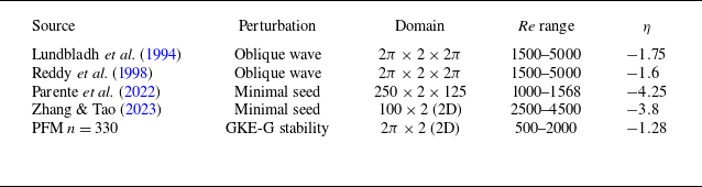
4. Conclusion
Due to the subcritical nature of the most shear flows, the calculation of the allowable perturbation level is an important scientific challenge. Minimal seed calculations by nonlinear optimisation have proven to be an efficient tool for that; however, the validation of the result still needs alternative methods. This study introduces an approach for determining the conditional stability limit of laminar flows by constructing a quadratic Lyapunov function. The method of Nerli et al. (Reference Nerli, Camarri and Salvetti2007) is followed to validate the Lyapunov function through nonlinear optimisation; however, in this study, it is defined in a more general form by applying a linear transformation to the state variables and establishing a generalised kinetic energy via the inner product of the transformed variables.
The transformation directly impacts the growth rate of generalised kinetic energy, making it dependent on the perturbation amplitude. This dependency allows for the calculation of the threshold amplitude of stability, offering vital insights into the system’s dynamics. With a suitable definition of the generalised kinetic energy through the transformation matrix, the maximum potential growth rate of infinitesimal perturbations is negative (if $\textit{Re} \lt \textit{Re}_L$
) and it increases with the perturbation level. The maximum potential growth rate of the system, relative to the perturbation level, delineates two distinct regions: an initial phase dominated by a linear dynamics at lower perturbation levels, followed by a transitional phase to a regime where nonlinear effects predominate at higher levels. The critical perturbation level, below which the laminar state remains stable, is defined by the intersection of the maximum generalised kinetic energy growth rate with the zero line.
$\textit{Re} \lt \textit{Re}_L$
) and it increases with the perturbation level. The maximum potential growth rate of the system, relative to the perturbation level, delineates two distinct regions: an initial phase dominated by a linear dynamics at lower perturbation levels, followed by a transitional phase to a regime where nonlinear effects predominate at higher levels. The critical perturbation level, below which the laminar state remains stable, is defined by the intersection of the maximum generalised kinetic energy growth rate with the zero line.
In the transformed state space, the basin of attraction is a hypersphere with a radius equal to the critical perturbation level, whereas, in the original state space, it is a hyperellipsoid with the smallest semiminor axis dictating the maximum allowable perturbation kinetic energy. To optimise this threshold, two strategies are delineated: the GKE-SV method, which optimises the singular values of the linear system’s eigenvector matrix, and the GKE-G method, which optimises the elements of a general triangular transformation matrix through the interior-point algorithm, utilising analytic gradients for efficiency.
A crucial part of the calculations involves determining the global maximum of the potential growth rate across a variety of perturbation states. To ensure precision, this methodology integrates the use of analytic gradients and the Hessian matrix, alongside employing multiple seed locations for a thorough exploration of the solution space. In this context, three renowned optimisation algorithms were evaluated, with the SQP method and the interior-point algorithm recommended for small and large dynamical systems, respectively.
When juxtaposed with traditional SOS programs, it emerges that the presented GKE methods give no significant benefits for smaller systems. However, they prove to be viable for larger systems, where $n \gt 20$
, a domain where SOS methods typically falter.
$n \gt 20$
, a domain where SOS methods typically falter.
The GKE-G method was applied to the well-known low-dimensional systems: the TTRD’ model and three different variations of the four-dimensional Waleffe model. In general, the proposed method predicts a similar allowable threshold amplitude as the SOS methods and significantly larger than so-called QC method. Additionally, for the TTRD’ model and the W95B and BT parameter sets of the Waleffe model, the proximity of the minimal seed solutions to the boundary of the calculated ROA reinforces the accuracy of the GKE-G methodology.
Applying GKE methods to a reduced-order model of two-dimensional Poiseuille flow (90–990 degrees of freedom) shows that the GKE-G method accurately calculates the perturbation threshold with 330 modes. Moreover, the calculated critical perturbation shape qualitatively aligns with minimal seed solutions from the literature.
The GKE-SV method predicts a much lower threshold amplitude at a fraction of the computational cost, with the divergence increasing at higher Reynolds numbers but staying within two orders of magnitude, even for the largest systems analysed.
In summary, the presented methodology for constructing quadratic Lyapunov functions can be applied to significantly larger fluid dynamical systems than SOS techniques. Nonetheless, challenges persist in three-dimensional domains due to the reliance on high-dimensional models. Employing more efficient basis functions, like controllability modes (Cavalieri & Nogueira Reference Cavalieri and Nogueira2022) instead of Stokes modes, could reduce the necessary model order, potentially enabling the analysis of finite-dimensional models for three-dimensional flows with the presented GKE methods. Future improvements might involve the use of infinite-dimensional models (Goulart & Chernyshenko Reference Goulart and Chernyshenko2012; Fuentes et al. Reference Fuentes, Goluskin and Chernyshenko2022), considering the worst-case effects of truncated modes on flow stability. Notably, Fuentes et al. (Reference Fuentes, Goluskin and Chernyshenko2022) demonstrated a significantly higher global stability limit for two-dimensional Couette flow using only 13 modes. Given that the GKE method can efficiently handle systems with several hundred modes, extending it to accommodate infinite-dimensional models could potentially uncover the conditional stability of physically relevant three-dimensional flows.
Acknowledgements.
The author is grateful to Y. Duguet at CNRS and David Goluskin at University of Victoria for their helpful recommendations. Furthermore, the author would like to express their sincere gratitude to the anonymous reviewers for their insightful comments, constructive suggestions and valuable time dedicated to reviewing this manuscript. Their feedback has significantly contributed to improving the clarity and quality of this work.
Funding.
This paper was supported by the János Bolyai Research Scholarship of the Hungarian Academy of Sciences. The research leading to these results received funding from the National Research Development and Innovation Office of Hungary under Grant Agreement no. K142675.
Declaration of interests.
The author reports no conflict of interest.
Appendix A. Numerical methods
A.1.
The maximisation of
$\mu _{h}$

The critical aspect of the method lies in determining the maximum potential growth rate of GKE (2.24). In practical implementations, Matlab’s fmincon is employed, a tool that can significantly benefit from the provision of gradient and Hessian matrix of the cost function. The derivatives of the growth rate (2.23) concerning the normalised state vector ( $\tilde {r}_k$
) are expressed as follows:
$\tilde {r}_k$
) are expressed as follows:
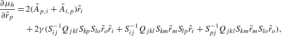 \begin{align} \frac {\partial \mu _h}{\partial \tilde {r}_p} &= 2\big (\tilde {A}_{p,i}+ \tilde {A}_{i,p}\big)\tilde {r}_i \nonumber \\ &\quad+2\gamma \big ( S_{ij}^{-1} Q_{jkl} S_{kp} S_{lo}\tilde {r}_o \tilde {r}_i + S_{ij}^{-1} Q_{jkl} S_{km}\tilde {r}_m S_{lp}\tilde {r}_i + S_{pj}^{-1} Q_{jkl} S_{km}\tilde {r}_m S_{lo}\tilde {r}_o \big ) ,\end{align}
where $\tilde {A}_{ij}$
is the transformed
$\tilde {A}_{ij}$
is the transformed $A_{ij}$
matrix defined in equation (2.19). Let us introduce the vectors
$A_{ij}$
matrix defined in equation (2.19). Let us introduce the vectors $v_j = S^{-T}_{ji}\tilde {r}_i$
and
$v_j = S^{-T}_{ji}\tilde {r}_i$
and $\tilde {q}_i = S_{ij}\tilde {r}_j$
to simplify the gradient
$\tilde {q}_i = S_{ij}\tilde {r}_j$
to simplify the gradient
 \begin{equation} \frac {\partial \mu _h}{\partial \tilde {r}_p} = 2\big (\tilde {A}_{pi}+ \tilde {A}_{ip}\big )\tilde {r}_i +2\gamma \big ( S_{pk}^{T} Q_{jkl} \tilde {q}_{l} v_j + S_{pl}^{T} Q_{jkl} \tilde {q}_{k} v_j + S_{pj}^{-1} Q_{jkl} \tilde {q}_{k} \tilde {q}_l \big ). \end{equation}
The Hessian matrix of $\mu _h$
(2.23) is given by
$\mu _h$
(2.23) is given by
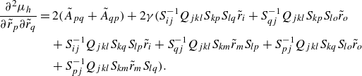 \begin{align} \frac {\partial ^2\mu _h}{\partial \tilde {r}_p\partial \tilde {r}_q} &= 2\big (\tilde {A}_{pq}+ \tilde {A}_{qp}\big ) + 2\gamma \big ( S_{ij}^{-1} Q_{jkl} S_{kp} S_{lq}\tilde {r}_i + S_{qj}^{-1} Q_{jkl} S_{kp} S_{lo}\tilde {r}_o \nonumber \\ &\quad +S_{ij}^{-1} Q_{jkl} S_{kq} S_{lp}\tilde {r}_i + S_{qj}^{-1} Q_{jkl} S_{km}\tilde {r}_m S_{lp} + S_{pj}^{-1} Q_{jkl} S_{kq} S_{lo}\tilde {r}_{o} \nonumber \\ &\quad + S_{pj}^{-1} Q_{jkl} S_{km} \tilde {r}_{m} S_{lq} \big ). \end{align}
By introducing the expressions
 \begin{equation} B_{kl} = Q_{jkl} v_j, \,\;\, C_{jk} = Q_{jkl} \tilde {q}_l, \,\;\, D_{jl} = Q_{jkl} \tilde {q}_k, \end{equation}
the equation (A3) simplifies to
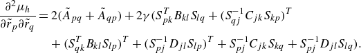 \begin{align} \frac {\partial ^2\mu _h}{\partial \tilde {r}_p\partial \tilde {r}_q} &= 2\big (\tilde {A}_{pq}+ \tilde {A}_{qp}\big )+ 2\gamma \big ( S_{pk}^{T} B_{kl} S_{lq} + \big (S_{qj}^{-1} C_{jk} S_{kp}\big )^T \nonumber \\ &\quad + \big (S_{qk}^{T} B_{kl} S_{lp}\big )^T + \big (S_{pj}^{-1} D_{jl} S_{lp}\big )^T + S_{pj}^{-1} C_{jk} S_{kq} + S_{pj}^{-1} D_{jl} S_{lq} \big ) .\end{align}
It is worth noticing that the Hessian matrix consists of the sum of four matrices and their transposes, resulting in a symmetric expression. This symmetry is expected due to the nature of second derivatives. From a practical perspective, only half of the expression needs to be calculated; the other half can be obtained by transposing the appropriate matrices.
The optimisation is constrained by the requirement that the transformed state vector should be unitary
 \begin{equation} c = \tilde {r}_i \tilde {r}_i - 1 = 0 .\end{equation}
The gradient of the constraint is straightforward
 \begin{equation} \frac {\partial c}{\partial \tilde {r}_i} = 2 \tilde {r}_i. \end{equation}
The Hessian of the constraint (A6) is given by
 \begin{equation} \frac {\partial ^2c}{\partial \tilde {r}_i \partial \tilde {r}_j} = 2 \delta _{i,j} ,\end{equation}
where $\delta _{i,j}$
is the Kronecker delta function and the right-hand side is two times the identity matrix.
$\delta _{i,j}$
is the Kronecker delta function and the right-hand side is two times the identity matrix.
A.2.
The maximisation of
$e_{{min}}$

The maximisation of $e_{{min}}(S_{ij})$
(2.30) through the GKE-G method is substantially enhanced by employing gradient-based optimisation. The sensitivity of
$e_{{min}}(S_{ij})$
(2.30) through the GKE-G method is substantially enhanced by employing gradient-based optimisation. The sensitivity of $e_{{min}}$
to variations in the transformation matrix is derived from equation (2.30) as
$e_{{min}}$
to variations in the transformation matrix is derived from equation (2.30) as
 \begin{equation} \frac {\partial e_{{min}}}{\partial S_{ij}}= 2\gamma _{{crit}} \frac {\partial \gamma }{\partial S_{ij}}\lambda _{{min}} + \gamma _{{crit}}^2 \frac {\partial \lambda _{{min}}}{\partial S_{ij}}. \end{equation}
The sensitivity of the $\lambda$
can be expressed as
$\lambda$
can be expressed as
 \begin{equation} \frac {\partial \lambda }{\partial S_{ij}}= 2 S_{ik} r_{{min},j} r_{{min},k} ,\end{equation}
where $\boldsymbol{r}_{{min}}$
is the eigenvector associated with the smallest eigenvalue of
$\boldsymbol{r}_{{min}}$
is the eigenvector associated with the smallest eigenvalue of $\textbf {S}^T\textbf {S}$
. The gradient of
$\textbf {S}^T\textbf {S}$
. The gradient of $\gamma$
with respect to the transformation matrix is determined as
$\gamma$
with respect to the transformation matrix is determined as
 \begin{equation} \frac {\partial \gamma }{\partial S_{ij}} = -\frac {\partial \mu _{h,{max}}}{\partial S_{ij}}\frac {1}{\dfrac {\partial \mu }{\partial \gamma }}. \end{equation}
The derivatives of the growth rate (2.26) with respect to the elements of the transformation matrix are calculated as follows:
 \begin{align} \frac {\partial \mu _{h,{max}}}{\partial S_{pq}} &= 2\big ( -\tilde {r}_i S_{ip}^{-1}S_{qj}^{-1} A_{jm} S_{mo}\tilde {r}_o + \tilde {r}_i S_{ij}^{-1}A_{jp} \tilde {r}_q \big )\nonumber \\ &\quad +2\gamma \big ( -\tilde {r}_i S_{ip}^{-1}S_{ql}^{-1} Q_{lmo} S_{mp} \tilde {r}_p S_{or} \tilde {r}_r +\tilde {r}_i S_{ij}^{-1} Q_{jpl} \tilde {r}_q S_{lo} \tilde {r}_o \nonumber \\ &\quad +\, \tilde {r}_i S_{ij}^{-1} Q_{jkp} S_{km} \tilde {r}_m \tilde {r}_q \big ), \end{align}
where it was assumed the inverse of a slightly perturbed transformation matrix can be approximated as
 \begin{equation} \big (S_{ij} + \delta S_{ij} \big )^{-1} \approx S_{ij}^{-1} - S_{ik}^{-1}\,\delta S_{kl}\, S_{lj}^{-1}. \end{equation}
Simplifying these expressions (A12) using predefined vectors and the transformed $A_{ij}$
results in
$A_{ij}$
results in
 \begin{align} \frac {\partial \mu _{h,{max}}}{\partial S_{pq}} &= 2\big ( -{v}_p \tilde {A}_{qj}\tilde {r}_j + v_j A_{jp} \tilde {r}_q \big )\nonumber \\ &\quad +2\gamma \big ( -{v}_p S_{ql}^{-1} Q_{lmo} \tilde {q}_m \tilde {q}_o +v_j Q_{jpl} \tilde {r}_q \tilde {q}_l + v_j Q_{jkp} \tilde {q}_k \tilde {r}_q \big ) .\end{align}
Moreover, the derivative of the growth rate with respect to the perturbation level is
 \begin{equation} \frac {\partial \mu _{h,{max}}}{\partial \gamma } = 2\, \gamma \, \tilde {Q}_{ijk}\,\tilde {r}_i\, \tilde {r}_j\,\tilde {r}_k , \end{equation}
which is simply the nonlinear component of $\mu _h$
 \begin{equation} \frac {\partial \mu _{h,{max}}}{\partial \gamma } = \mu _{h,{NL}}. \end{equation}
The derivatives presented in equations (A14) and (A15) are evaluated at the critical perturbation that maximises the growth rate, $\mu _{h}$
.
$\mu _{h}$
.
A.2.1. First sum-of-squares program
The first (SOS) program, widely used to calculate the ROA for conditionally stable systems (Jarvis-Wloszek Reference Jarvis-Wloszek2003; Tan & Packard Reference Tan and Packard2008; Topcu et al. Reference Topcu, Packard and Seiler2008; Khodadadi et al. Reference Khodadadi, Samadi and Khaloozadeh2014; Kalur et al. Reference Kalur, Seiler and Hemati2021), is delineated as follows:
 \begin{align}&\qquad\qquad V - l_1 \in \Sigma ,\end{align}
 \begin{align}&\, -\big [(\beta -p)s_1 + (V-{\gamma ^2})\big ] \in \Sigma, \end{align}
 \begin{align}& -\big (({\gamma ^2}-V)s_2 + \dot {V}\,s_3 + l_2\big ) \in \Sigma . \end{align}
The following three paragraphs provide a brief description of the method, along with the new expressions and notations. Here, $V$
represents the conditional Lyapunov function, akin to
$V$
represents the conditional Lyapunov function, akin to $h$
in the GKE method but potentially non-quadratic, contrasting with the strictly quadratic nature of
$h$
in the GKE method but potentially non-quadratic, contrasting with the strictly quadratic nature of $h$
in the GKE method. The derivative of
$h$
in the GKE method. The derivative of $V$
with respect to time is denoted as
$V$
with respect to time is denoted as $\dot {V}$
 \begin{equation} \dot {V} = \frac {\partial V}{\partial q_i}\, \frac {\mathrm{d}q_i}{\mathrm{d}t}. \end{equation}
The polynomials $l_1$
and
$l_1$
and $l_2$
are predefined positive definite to ensure positive definiteness (rather than semi-definiteness) of the expressions, set to
$l_2$
are predefined positive definite to ensure positive definiteness (rather than semi-definiteness) of the expressions, set to $l_i = 10^{-10}\boldsymbol{q}^T \boldsymbol{q}$
for minimal impact on results. The variable
$l_i = 10^{-10}\boldsymbol{q}^T \boldsymbol{q}$
for minimal impact on results. The variable $\beta$
indicates the ROA’s size, with
$\beta$
indicates the ROA’s size, with $p$
depicting its shape, typically chosen as
$p$
depicting its shape, typically chosen as $p=\boldsymbol{q}^T \boldsymbol{q}$
to describe a supersphere, thus approximating the ROA similar to the generalised kinetic energy methods with
$p=\boldsymbol{q}^T \boldsymbol{q}$
to describe a supersphere, thus approximating the ROA similar to the generalised kinetic energy methods with $\beta =e_{{min}}$
. The parameter
$\beta =e_{{min}}$
. The parameter $\gamma$
specifies the state space region where the Lyapunov function decreases along the system’s solution trajectories.
$\gamma$
specifies the state space region where the Lyapunov function decreases along the system’s solution trajectories.
Equation (A17) asserts that the Lyapunov function $V$
must be positive definite. Equation (A18) is employed to maximise
$V$
must be positive definite. Equation (A18) is employed to maximise $\beta$
for the largest possible ROA shaped by the polynomial
$\beta$
for the largest possible ROA shaped by the polynomial $p$
. Equation (A19) mandates that the Lyapunov function decreases along the solution trajectories within the region where
$p$
. Equation (A19) mandates that the Lyapunov function decreases along the solution trajectories within the region where $V\lt {\gamma ^2}$
. The symbols
$V\lt {\gamma ^2}$
. The symbols $s_1, s_2, s_3$
represent positive semi-definite polynomials.
$s_1, s_2, s_3$
represent positive semi-definite polynomials.
The notation ‘ $\in \Sigma$
’ signifies that the left-hand side must be expressible in a SOS form, thereby being positive semi-definite. A SOS decomposition enables a polynomial up to degree
$\in \Sigma$
’ signifies that the left-hand side must be expressible in a SOS form, thereby being positive semi-definite. A SOS decomposition enables a polynomial up to degree $2d$
to be represented as
$2d$
to be represented as $\boldsymbol{m}^T(\boldsymbol{q})\,\textbf {M}\,\boldsymbol{m}(\boldsymbol{q})$
, with
$\boldsymbol{m}^T(\boldsymbol{q})\,\textbf {M}\,\boldsymbol{m}(\boldsymbol{q})$
, with $\boldsymbol{m}(\boldsymbol{q})$
encompassing all monomials up to order
$\boldsymbol{m}(\boldsymbol{q})$
encompassing all monomials up to order $d$
and
$d$
and $\textbf {M}$
a positive definite matrix, leading to matrix inequality constraints during optimisation. While the problem could be reformulated into a SDP solvable efficiently if all constraints were linear, equations (A18–A19) include bilinear terms in polynomial decision variables, necessitating a decomposed optimisation approach over multiple iterations. Initially, the process starts with the
$\textbf {M}$
a positive definite matrix, leading to matrix inequality constraints during optimisation. While the problem could be reformulated into a SDP solvable efficiently if all constraints were linear, equations (A18–A19) include bilinear terms in polynomial decision variables, necessitating a decomposed optimisation approach over multiple iterations. Initially, the process starts with the $\gamma$
step, during which
$\gamma$
step, during which $\gamma$
is treated as a parameter rather than as part of the decision variables. This parameter is maximised using a bisection algorithm until equation (A19) is feasible, indicating that the left-hand side can be represented as a SOS expression. Following this, the
$\gamma$
is treated as a parameter rather than as part of the decision variables. This parameter is maximised using a bisection algorithm until equation (A19) is feasible, indicating that the left-hand side can be represented as a SOS expression. Following this, the $\beta$
step commences, setting
$\beta$
step commences, setting $\beta$
as a parameter and employing a bisection algorithm to maximise it until equation (A18) is satisfied, using the maximal
$\beta$
as a parameter and employing a bisection algorithm to maximise it until equation (A18) is satisfied, using the maximal $\gamma$
value determined in the previous step. The final phase is the
$\gamma$
value determined in the previous step. The final phase is the $V$
step, where all equations from (A17) to (A19) are addressed. However, in this phase, decision variables established in earlier steps are held constant, with the exception of the Lyapunov function
$V$
step, where all equations from (A17) to (A19) are addressed. However, in this phase, decision variables established in earlier steps are held constant, with the exception of the Lyapunov function $V$
, which undergoes updates. This sequence of steps is iterated until
$V$
, which undergoes updates. This sequence of steps is iterated until $\beta$
reaches its peak, and the relative change dips below the set tolerance level of
$\beta$
reaches its peak, and the relative change dips below the set tolerance level of $10^{-3}$
. This iterative algorithm is designated as SOS1 in this study.
$10^{-3}$
. This iterative algorithm is designated as SOS1 in this study.
A.2.2. Second sum-of-squares program
In the context of quadratic Lyapunov functions, an alternative approach has been proposed by Liu & Gayme (Reference Liu and Gayme2020). This approach adopts the same definition of the Lyapunov function as in the GKE method, with $V=h$
, as outlined in equation (2.14). The corresponding SOS program is presented as follows:
$V=h$
, as outlined in equation (2.14). The corresponding SOS program is presented as follows:
 \begin{align}&\qquad\qquad V - l_1 \in \Sigma ,\end{align}
 \begin{align}& -\big (\dot {V} + (\delta ^2 - \boldsymbol{q}^T \boldsymbol{q})s_1 +l_2\big ) \in \Sigma .\end{align}
The first equation (A21) ensures the positive definiteness of the Lyapunov function ( $V$
), analogous to equation (A17). The subsequent equation, (A22), mandates that
$V$
), analogous to equation (A17). The subsequent equation, (A22), mandates that $\dot {V}$
is negative within a specific region, the size of which is proportional to
$\dot {V}$
is negative within a specific region, the size of which is proportional to $\delta ^2$
. However, this region is not the ROA since, although
$\delta ^2$
. However, this region is not the ROA since, although $\dot {V} \lt 0$
,
$\dot {V} \lt 0$
, $d/{\rm d}t (||q||)$
can be positive in this region and trajectories can go outwards. The provable ROA is a subset of this region where
$d/{\rm d}t (||q||)$
can be positive in this region and trajectories can go outwards. The provable ROA is a subset of this region where $V\lt \gamma ^2$
. Here,
$V\lt \gamma ^2$
. Here, $\gamma$
can be calculated from the definition of
$\gamma$
can be calculated from the definition of $V$
as
$V$
as $\gamma ^2 = \lambda _{{min}}(P) \, \delta ^2$
. This approach replaces and simplifies the second equation (A18) of SOS1 leading to faster but less accurate results.
$\gamma ^2 = \lambda _{{min}}(P) \, \delta ^2$
. This approach replaces and simplifies the second equation (A18) of SOS1 leading to faster but less accurate results.
The calculated ROA forms a superellipsoid analogous to that in the GKE method. The radius of the largest supersphere contained within this superellipsoid is given by ${\sqrt {e_{{min}}}} = \delta \sqrt {\lambda _{{min}}(P)/\lambda _{{max}}(P)}$
.
${\sqrt {e_{{min}}}} = \delta \sqrt {\lambda _{{min}}(P)/\lambda _{{max}}(P)}$
.
Like SOS1, (A22) introduces a nonlinear constraint on the decision variables due to the inclusion of the term $\delta ^2 \,s_1$
. To address this,
$\delta ^2 \,s_1$
. To address this, $\delta ^2$
is considered as a parameter rather than a decision variable and is maximised using a bisection algorithm until (A22) is feasible. This SOS program is referred to as SOS2 in the study.
$\delta ^2$
is considered as a parameter rather than a decision variable and is maximised using a bisection algorithm until (A22) is feasible. This SOS program is referred to as SOS2 in the study.
Appendix B. Construction of Poiseuille flow model
The Stokes equations in non-dimensional form are given by
 \begin{equation} \frac {\partial {u}_{i}}{\partial t}=-\frac {\partial {p}}{\partial x_i}+\frac {1}{\textit{Re}}\frac {\partial ^2 {u}_i}{\partial x_j \partial x_j} ,\end{equation}
and
 \begin{equation} \frac {\partial {u}_{i}}{\partial x_i}=0, \end{equation}
where ${u}_{i}$
represents the non-dimensional velocity,
${u}_{i}$
represents the non-dimensional velocity, $p$
is the non-dimensional pressure and
$p$
is the non-dimensional pressure and $x_i$
are the spatial coordinates:
$x_i$
are the spatial coordinates: $x_1\in [0,L_x]; \, x_2\in [-1,1]; \,x_3\in [0,L_z]$
, defining a rectangular cuboid. The eigenvectors can be obtained by assuming the following ansatz:
$x_1\in [0,L_x]; \, x_2\in [-1,1]; \,x_3\in [0,L_z]$
, defining a rectangular cuboid. The eigenvectors can be obtained by assuming the following ansatz:
 \begin{equation} u_i = \hat {u}_{i} \mathrm{e}^{ \lambda \,t } ,\end{equation}
and solving the eigenvalue problem
 \begin{align}& \lambda \hat {u}_{i}=-\frac {\partial \hat {p}}{\partial x_i}+\frac {1}{\textit{Re}}\frac {\partial ^2 \hat {u}_i}{\partial x_j \partial x_j}, \end{align}
 \begin{align}&\qquad\qquad {\frac {\partial \hat {u}_{i}}{\partial x_i}=0} ,\end{align}
for $\lambda$
. The eigenvalues are negative real numbers expressing the dissipation rate of the mode. Furthermore, the eigenvectors are orthogonal, which proves advantageous for Galerkin projection. Given the linearity of the eigenvalue problem and assuming periodic solutions in the
$\lambda$
. The eigenvalues are negative real numbers expressing the dissipation rate of the mode. Furthermore, the eigenvectors are orthogonal, which proves advantageous for Galerkin projection. Given the linearity of the eigenvalue problem and assuming periodic solutions in the $x_1$
and
$x_1$
and $x_3$
directions, solving the eigenvalue problem is conveniently achieved using complex Fourier series. The modes of the
$x_3$
directions, solving the eigenvalue problem is conveniently achieved using complex Fourier series. The modes of the $\hat {u}_i$
velocity field can be expressed as follows:
$\hat {u}_i$
velocity field can be expressed as follows:
 \begin{equation} \tilde {u}_{i\, j_m\,k_m}(x_2)\mathrm{e}^{ \mathrm{i}(j_m \alpha _0 x_1 + k_m \beta _0 x_3)}, \end{equation}
where $\alpha _0 = 2 \pi / L_x$
and
$\alpha _0 = 2 \pi / L_x$
and $\beta _0 = 2 \pi / L_z$
are the wavenumbers, and
$\beta _0 = 2 \pi / L_z$
are the wavenumbers, and $j_m$
,
$j_m$
, $k_m$
are the indices of the modes ranging from
$k_m$
are the indices of the modes ranging from $-\infty$
to
$-\infty$
to $\infty$
. Substituting the complex wave form (B6) into equations (B2) and (B4) leads to the following eigenvalue problem for each
$\infty$
. Substituting the complex wave form (B6) into equations (B2) and (B4) leads to the following eigenvalue problem for each $j_m, k_m$
mode
$j_m, k_m$
mode
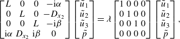 \begin{equation} \begin{bmatrix} L & 0 & 0 & -\mathrm{i}\alpha \\ 0 & L & 0 & -D_{x_2}\\ 0 & 0 & L & -\mathrm{i}\beta \\ \mathrm{i}\alpha & D_{x_2} & \mathrm{i}\beta & 0 \end{bmatrix} \begin{bmatrix}\tilde {u}_1\\\tilde {u}_2\\\tilde {u}_3\\\tilde {p} \end{bmatrix} = \lambda \begin{bmatrix} 1 & 0 & 0 & 0\\ 0 & 1 & 0 & 0\\ 0 & 0 & 1 & 0\\ 0 & 0 & 0 & 0 \end{bmatrix} \begin{bmatrix}\tilde {u}_1\\\tilde {u}_2\\\tilde {u}_3\\\tilde {p} \end{bmatrix}, \end{equation}
where $\alpha = j_m\, \alpha _0$
,
$\alpha = j_m\, \alpha _0$
, $\beta = k_m\, \beta _0$
and
$\beta = k_m\, \beta _0$
and $L = -(\alpha ^2+\beta ^2) + D_{x_2}^2$
is the Laplace operator, where
$L = -(\alpha ^2+\beta ^2) + D_{x_2}^2$
is the Laplace operator, where $D_{x_2}$
is the differential operator with respect to
$D_{x_2}$
is the differential operator with respect to $x_2$
.
$x_2$
.
The problem (B7) can be discretised using the Chebyshev collocation method. The required boundary conditions involve stationary walls at the bottom and top of the domain, implying $\tilde {u}_i(\pm 1) = 0$
for any
$\tilde {u}_i(\pm 1) = 0$
for any $i$
velocity component. These conditions are enforced by removing the corresponding rows from the matrices. In this study, 100 Chebyshev collocation points are employed, a choice deemed accurate based on prior research (Nagy & Kulcsár Reference Nagy and Kulcsár2023). The discretised version of the equations (B7) solved for the first
$i$
velocity component. These conditions are enforced by removing the corresponding rows from the matrices. In this study, 100 Chebyshev collocation points are employed, a choice deemed accurate based on prior research (Nagy & Kulcsár Reference Nagy and Kulcsár2023). The discretised version of the equations (B7) solved for the first $N_y$
modes with the largest
$N_y$
modes with the largest $\lambda$
eigenvalues for
$\lambda$
eigenvalues for $j_m \in [-N_x,N_x]$
and
$j_m \in [-N_x,N_x]$
and $k_m \in [-N_z,N_z]$
resulting in a total of
$k_m \in [-N_z,N_z]$
resulting in a total of $n = (2N_x+1)\, N_y\, (2N_z+1)$
modes. The calculation can be simplified, since in the case of complex-conjugate wavenumber pairs (
$n = (2N_x+1)\, N_y\, (2N_z+1)$
modes. The calculation can be simplified, since in the case of complex-conjugate wavenumber pairs ( $j_{m, a} = -j_{m, b}$
and
$j_{m, a} = -j_{m, b}$
and $k_{m, a} = -k_{m, b}$
), the eigenvalues are the same and the eigenvectors are the complex conjugate of each other
$k_{m, a} = -k_{m, b}$
), the eigenvalues are the same and the eigenvectors are the complex conjugate of each other $\tilde {u}^{}_{i\,j_m\,k_m}=\tilde {u}^*_{i\,-j_m\,-k_m}$
. The values of the parameters (
$\tilde {u}^{}_{i\,j_m\,k_m}=\tilde {u}^*_{i\,-j_m\,-k_m}$
. The values of the parameters ( $N_x, N_y,N_z$
) vary across different models and will be provided later. Subsequently, the coefficients
$N_x, N_y,N_z$
) vary across different models and will be provided later. Subsequently, the coefficients $A_{ij}$
and
$A_{ij}$
and $Q_{ij k}$
are computed using the Galerkin projection method
$Q_{ij k}$
are computed using the Galerkin projection method
 \begin{align}& A_{i_m\,j_m} = \int _\varOmega \left(-{U}_{j}\frac {\partial \hat {u}_{i\, i_m}}{\partial x_j}-\hat {u}_{j\, i_m}\frac {\partial {U}_{i}}{\partial x_j}+\frac {1}{\textit{Re}}\frac {\partial ^2 {u}_{i\, i_m}}{\partial x_j \partial x_j}\right) \hat {u}^*_{i\, j_m} \mathrm{d} \varOmega,\\[-8pt]\nonumber \end{align}
 \begin{align}&\qquad\qquad\quad Q_{i_m j_m k_m} = \int _\varOmega \left(-\hat {u}_{j\, j_m}\frac {\partial \hat {u}_{i\, i_m}}{\partial x_j}\right) \hat {u}^*_{i\, k_m} \mathrm{d} \varOmega , \end{align}
where $i_m,j_m$
and
$i_m,j_m$
and $k_m$
are the indices of the modes,
$k_m$
are the indices of the modes, ${U}_{i}$
denotes the velocity field of the base flow and
${U}_{i}$
denotes the velocity field of the base flow and $\hat {u}^*_{i\, j_m}$
is the complex conjugate of
$\hat {u}^*_{i\, j_m}$
is the complex conjugate of $\hat {u}^*_{i\, j_m}$
. For the Poiseuille flow investigated in this study, having only one non-zero velocity component
$\hat {u}^*_{i\, j_m}$
. For the Poiseuille flow investigated in this study, having only one non-zero velocity component
 \begin{equation} U_1 = 1-x_2^2. \end{equation}
It is worth noting that
 \begin{equation} \int _\varOmega \frac {\partial ^2 {u}_{i\, i_m}}{\partial x_j \partial x_j} \hat {u}^*_{i\, j_m} \mathrm{d} \varOmega = \lambda _{i_m}\, \delta _{i_m,j_m} .\end{equation}
This is due to the fact that the velocity modes are eigensolutions of the Stokes operator, equations (B4) and (B5).
The modes are substituted in the form (B6) and the integrals over $x_2$
are evaluated utilising Chebyshev collocation points. Since the eigenvectors are complex, the
$x_2$
are evaluated utilising Chebyshev collocation points. Since the eigenvectors are complex, the $A_{ij}$
matrix and the
$A_{ij}$
matrix and the $Q_{ijk}$
tensor are also complex. As a result, the previously derived gradients for the optimisation procedure become invalid. However, this issue can be resolved by transforming the system into a real-valued one. Let
$Q_{ijk}$
tensor are also complex. As a result, the previously derived gradients for the optimisation procedure become invalid. However, this issue can be resolved by transforming the system into a real-valued one. Let $i_0$
represent the indices of the real-valued modes,
$i_0$
represent the indices of the real-valued modes, $i_c$
the complex-valued modes and
$i_c$
the complex-valued modes and $i_{cc}$
their corresponding complex conjugates. By rearranging the modes in the order
$i_{cc}$
their corresponding complex conjugates. By rearranging the modes in the order $i_0, i_c, i_{cc}$
, a transformation matrix
$i_0, i_c, i_{cc}$
, a transformation matrix $\textbf {T}$
can be defined as follows:
$\textbf {T}$
can be defined as follows:
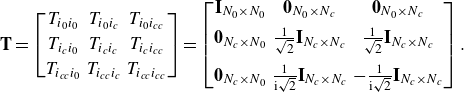 \begin{equation} \textbf {T} = \begin{bmatrix} T_{i_0 i_0} & T_{i_0 i_c} & T_{i_0 i_{cc}}\\[3pt] T_{i_c i_0} & T_{i_c i_c} & T_{i_c i_{cc}}\\[3pt] T_{i_{cc} i_0} & T_{i_{cc} i_c} & T_{i_{cc} i_{cc}}\\ \end{bmatrix}= \begin{bmatrix} \textbf {I}_{N_0\times N_0} & \textbf {0}_{N_0\times N_c} & \textbf {0}_{N_0\times N_c}\\[5pt] \textbf {0}_{N_c\times N_0} & \frac {1}{\sqrt {2}}\textbf {I}_{N_c\times N_c} & \frac {1}{\sqrt {2}}\textbf {I}_{N_c\times N_c}\\[9pt] \textbf {0}_{N_c\times N_0} & \frac {1}{\mathrm{i}\sqrt {2}}\textbf {I}_{N_c\times N_c} & -\frac {1}{\mathrm{i}\sqrt {2}}\textbf {I}_{N_c\times N_c}\\ \end{bmatrix}. \end{equation}
Here, $N_0$
represents the number of real-valued modes, and
$N_0$
represents the number of real-valued modes, and $N_c$
represents the number of complex-valued modes (taking into account half of the complex-conjugate pairs). Applying the
$N_c$
represents the number of complex-valued modes (taking into account half of the complex-conjugate pairs). Applying the $\textbf {S} = \textbf {T}^{-1}$
transformation matrix on the problem as described by equations (2.19) and (2.20) results in real-valued
$\textbf {S} = \textbf {T}^{-1}$
transformation matrix on the problem as described by equations (2.19) and (2.20) results in real-valued $A_{ij}$
matrix and the
$A_{ij}$
matrix and the $Q_{ijk}$
tensor, respectively. This transformation matrix can also be used to convert the transformed real coefficients back into the original complex coefficients of the complex-valued modes.
$Q_{ijk}$
tensor, respectively. This transformation matrix can also be used to convert the transformed real coefficients back into the original complex coefficients of the complex-valued modes.


 Open access