


1. Introduction
For tidal turbines in a channel or passage, an increase in the ratio between rotor swept area and channel cross-section, the blockage ratio, can lead to an increase in loads and potentially performance. Garrett & Cummins (Reference Garrett and Cummins2007) provided the first analytical assessment for tidal turbines in a channel, showing that for turbines homogeneously arrayed across a channel the theoretical limit of the power coefficient increases by  $1/(1-B)^{2}$, where $B$ is the blockage ratio. The majority of channels deemed suitable for commercial-scale tidal energy extraction are, however, much larger than typical rotor dimensions (Coles & Walsh Reference Coles and Walsh2019) and the resulting blockage ratios for low numbers of deployed turbines, and hence effect on turbine loads, are likely small. Turbine loads increase in blocked flow conditions due to the development of a streamwise pressure gradient, itself a result of confined wake expansion which causes the bypass flow to accelerate.
Although it may be desirable to install a large number of turbines with large frontal area in order to exploit blockage effects in channel flows, this may be impracticable due to physical constraints, i.e. bathymetric variations, operational requirements on the flow passage such as shipping, and the environmental impact of imposing such large resistances on the flow. A more practical solution is to use a co-planar fence of closely spaced turbines arrayed normally to the flow that partially spans the width of a much wider channel. Nishino & Willden (Reference Nishino and Willden2012) used a multi-scale analytic model to show that by reducing inter-turbine spacing for a fence of turbines, so-called constructive interference effects can be used to exploit local blockage effects between turbines, even for small global blockage. Nishino & Willden (Reference Nishino and Willden2013) extended this analytical model and conducted complimentary simulations for a partial fence, demonstrating similar results for more physically feasible and, hence, relevant tidal turbine fence systems.
Cooke et al. (Reference Cooke, Willden, Byrne, Stallard and Olczak2015) conducted experiments in a wide channel with porous disks to emulate turbines to explore the principles of the partial fence theory of Nishino & Willden (Reference Nishino and Willden2012) and determined that local constructive interference effects can be used to support higher disk thrusts in closely spaced arrays, leading to greater power extraction in the case of turbines. Scherl et al. (Reference Scherl, Strom, Brunton and Polagye2020) performed experiments for two vertical axis turbines varying the cross-stream and streamwise inter-turbine spacing in 64 different configurations. They concluded that a cross-stream arrangement, in which turbines are arrayed co-planar, provided the best performance enhancement, with diminishing performance as the streamwise separation increased and one turbine entered the wake of the other, relaxing local blockage effects.
By imparting thrust on the flow, a velocity deficit is created behind a tidal turbine together with an accompanying acceleration of the bypass flow outside of the turbine's swept area. These dynamics are of interest to those studying turbine wakes and their effect on performance to improve array design. Mycek et al. (Reference Mycek, Gaurier, Germain, Pinon and Rivoalen2014) considered the interaction between a tidal turbine and another placed downstream and on the same rotational axis. As expected, the downstream rotor experienced a lower performance than the upstream rotor due to a reduction in the oncoming flow speed, with the difference reducing with an increase in downstream spacing. Higher levels of ambient turbulence intensity were shown to increase mixing and aid wake recovery, thus reducing the detrimental effect on the downstream turbine's performance.
Experimental studies of larger numbers of rotors have been performed by Stallard et al. (Reference Stallard, Collings, Feng and Whelan2013) and Olczak et al. (Reference Olczak, Stallard, Feng and Stansby2016) through the use of 0.27 m diameter rotors. These studies considered one and two row arrays containing 1–10 turbines in a variety of arrangements, and demonstrated accelerated bypass flows jetting between rotors. For a staggered array of seven turbines with three upstream and four downstream rotors, Olczak et al. (Reference Olczak, Stallard, Feng and Stansby2016) observed the thrust loading on the downstream turbines was reduced compared with the front row, more so for the two rotors in the centre of the rear row due to the wakes of the upstream rotors merging to create a wider velocity deficit approaching these rotors. Malki et al. (Reference Malki, Masters, Williams and Nick Croft2014) used a blade-element method within a Reynolds-averaged Navier–Stokes solver (RANS-BE) to study various turbine layouts. They demonstrated a performance increase for a single turbine placed downstream and staggered between two upstream turbines. A similar configuration with three 1.2 m diameter turbines was demonstrated experimentally by Noble et al. (Reference Noble, Draycott, Nambiar, Sellar, Steynor and Kiprakis2020) who observed as much as a 10.4 % increase in power for the downstream rotor compared with its operation in isolation. These downstream rotor performance increases result from operation in the accelerated bypass flow of the upstream turbines.
Hunter, Nishino & Willden (Reference Hunter, Nishino and Willden2015) performed simulations using porous disks as a surrogate for tidal turbines to consider the effect of downstream spacing in a staggered array of two turbine rows. They demonstrated that although turbines experienced a performance uplift when operating in the bypass flow of upstream turbines, the maximum power attainable from a fence of seven turbines (four upstream, three downstream) was always achieved when all turbines were arrayed in a single cross-stream row rather than in a staggered formation. Performance was maximised in the co-planar array due to local blockage effects, and although the power of the downstream row increased as those turbines were moved rearward, this was negated by a greater drop in that of the upstream row, leading to overall lower performance. They observed that some, although not all, of the performance difference lost in the staggered formation, relative to the aligned formation, could be recovered by non-uniform control (resistances) of the turbines. This was different to their observations for the aligned row, where maximum performance was observed for turbines operating at the same control (local thrust) point.
An investigation into turbines designed for different blockage ratios was conducted by Schluntz & Willden (Reference Schluntz and Willden2015). They showed that deploying a given turbine design in a higher blockage than it was designed for leads to some performance benefits, but that further benefits were achievable through redesign of the turbine for the intended operational blockage. However, they also showed that operating a high-blockage-design turbine in a lower channel blockage could be detrimental to its performance, and that superior performance can be achieved by a turbine designed for that lower blockage. In order to fully exploit blockage effects, and by extension constructive interference effects in partial turbine fences, they concluded that rotors must be designed for operation in their intended configuration taking account of blockage and surface proximity effects.
Although the tidal turbine industry is now well-established, with a number of multi-megawatt devices from different developers being grid connected and deployed for extended periods (Coles & Walsh Reference Coles and Walsh2019), there remains a lack of industry experience for constructive interference to be considered in the design and manufacture of devices. That being said, a number of developers, e.g. Orbital Marine Power and SME-Schottel, are developing the types of multi-rotor systems whose designs could readily benefit from constructive interference considerations.
The wind energy industry has also explored multi-rotor systems, although there are distinct fluid mechanical differences between the two applications. The confinement of tidal flows between the seabed and free surface makes the conditions for constructive interference more attainable for the tidal energy industry, whereas wind turbines operate in flows with significantly reduced vertical confinement due to the very significantly greater distance (in turbine diameters) to the top of the atmospheric boundary layer. Furthermore, although tidal flows are largely bidirectional, the wind direction is variable and much less predictable, rendering closely spaced co-planar fence-type layouts unrealistic for wind flows in which wake interactions must be considered. van der Laan et al. (Reference van der Laan2019) describe power and wake measurements of the Vestas four-rotor wind turbine designed for research purposes. They demonstrated an overall power enhancement due to rotor interaction of 1.8 % and improved wake recovery at flow speeds below rated. van der Laan & Abkar (Reference van der Laan and Abkar2019) demonstrated that this can lead to increased energy yield in arrays, compared with conventional single-rotor turbines. The increased wake recovery was shown to benefit the power performance for a second downstream row. For subsequent rows, array level wake mixing dominated over turbine scale mixing and similar performance benefits were not possible.
In this study, we assess constructive interference for tidal turbines, by performing experiments to compare the loads and performance of a single turbine and an array of two side-by-side turbines. The following section describes the experimental method including the facility and turbine models. Detail and analysis of the flow measurements both with and without the turbines are presented in § 3, and § 4 describes analysis of the turbine data including accounting for global blockage. Results in § 5 describe both mean rotor and unsteady blade loading under a range of test conditions.
2. Experimental method
2.1. Test facility
The tests were conducted at FloWave (https://www.flowave.eng.ed.ac.uk/) at the University of Edinburgh, a 25 m diameter tank with pumps and wave paddles positioned around its circumference, able to generate current and waves in any direction. Sutherland et al. (Reference Sutherland, Noble, Steynor, Davey and Bruce2017) have quantified the velocity shear and turbulence at a range of conditions at the facility, providing depth profiles and turbulence quantities at a range of nominal flow speeds. Following their work, a flow speed of  $0.8\ {\rm m}\ {\rm s}^{-1}$ was chosen for the present test campaign so that comparisons could be made in the analysis. This relatively high flow speed was chosen so as to achieve as high a blade chord Reynolds number as possible, in the range $1.4 \unicode{x2013} 2 \times 10^5$ at an inflow speed of $0.8\ {\rm m} {\rm s}^{-1}$, to promote post-transitional blade flow. Details on the Reynolds number independence of the results that confirm $0.8\ {\rm m}\ {\rm s}^{-1}$ as a suitable flow speed are provided in Appendix A. At this tank flow speed the streamwise turbulence intensity is in the range of 6–8 % and the mean shear profile is well described by a power law with an exponent of one-sixth to one-ninth, varying spatially throughout the tank.
2.2. Turbine model
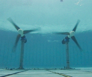
The tests used two identical three-bladed horizontal-axis tidal turbines with rotor diameter  $d = 1.2$ m, shown in figure 1. The rotors were designed specifically for the twin turbine configuration when deployed in this test facility, using a methodology that accounts for local blockage effects and provides superior rotor performance by exploiting constructive interference effects (Cao, Willden & Vogel Reference Cao, Willden and Vogel2018; Cao Reference Cao2020). A two-stage hydrodynamic rotor design process was performed; first using RANS-BE in which boundary and turbine proximity effects are accounted for through the computational stencil, which was then followed by blade resolved simulation using a moving reference frame method. The second stage is necessary to adjust the design for complex flows at the root and tip where lower-order RANS-BE solutions are less accurate. A full description of the hydrodynamic design method is given in Cao (Reference Cao2020).

Figure 1. Photograph of the twin tidal turbines during operation.
The rotors were mounted to existing drive-trains and nacelles provided by the University of Edinburgh. These drive-trains made use of a thrust and torque transducer upstream of the shaft bearing and seal arrangement, allowing loads to be measured without any mechanical losses. Further details of the nacelle and drive-train are given in Payne, Stallard & Martinez (Reference Payne, Stallard and Martinez2017), whereas details of the rotor manufacture and integration for these tests may be found in McNaughton et al. (Reference McNaughton, Cao, Vogel and Willden2019). The two turbines operated independently of each other and thus there was no phase locking between the blade azimuth positions. Further, owing to small fluctuations in the motor speeds the relative phase difference between the two turbines varied in time.
2.3. Test matrix
Tests were performed to characterise the flow in the absence of turbines, as well as two turbine configurations, single and twin. (Owing to project timescales the flow measurements without turbines were performed in May 2021 whereas the turbine tests were completed two years earlier in February 2019. For both experimental campaigns tank settings were the same and a comparison of data points performed during both campaigns is provided in Appendix B.) The turbine layouts are shown in figure 2. For clarity, the turbines are referred to as the North and South turbines, with the North turbine being the rotor used in both single and twin configurations, and the South turbine the additional rotor used only in the twin configuration.

Figure 2. (a) Schematic of FloWave layout (adapted from Noble et al. Reference Noble, Davey, Smith, Kaklis, Robinson and Bruce2015; Sutherland et al. Reference Sutherland, Noble, Steynor, Davey and Bruce2017) indicating layout of turbines, note that streamlines are illustrative only. (b) Turbine positions and naming conventions used in this study. Not to scale.
The turbines were positioned with their rotor plane 1.3 $d$ downstream of the mid plane of the tank, based on experience of previous tests such as Sutherland et al. (Reference Sutherland, Noble, Steynor, Davey and Bruce2017) to minimise spatial changes in flow conditions. The rotors were located at mid-water depth and for the twin configuration the tip-to-tip distance between the rotors was $s = d/4$ with the rotors symmetrical placed either side of the tank centreline. For practical reasons, the North turbine position did not change between single and twin configurations meaning that there was a minor asymmetry during the single turbine experiments. An additional asymmetry from both turbines rotating in the same direction was also present for the twin turbine case. This was due to the model design and ease of machining six identical blades rather than two sets of three. Although it is unlikely that this had noticeable effect on the mean interactional effects of the turbines, this asymmetry may have resulted in uneven loading or flow effects. Using counter-rotating turbines would have prevented this and provided an opportunity to better understand some of the blade loading effects discussed later in § 5.3.
The global blockage ratio (ratio of total frontal area of turbines to channel cross-sectional area),  $B_G$, and the local blockage ratio (ratio of a turbine's frontal area to the local flow passage cross-sectional area), $B_L$, are defined as
 \begin{equation} B_G = \frac{n A}{w h}, \quad B_L = \frac{A}{(s+d)h}, \end{equation}
with  $A$ the swept area of a single turbine's rotor, $w$ the channel width, $h$ the depth and $n$ the number of turbines. We adopt the definition of local blockage from Nishino & Willden (Reference Nishino and Willden2012) for consistency with previous works. Note that this definition takes no account of the aspect ratio of the local flow passage nor of anisotropy at turbine fence ends. Noble et al. (Reference Noble, Draycott, Nambiar, Sellar, Steynor and Kiprakis2020) presented details on the current generation properties of the test facility, demonstrating that the circumferentially placed pumps cause the mean flow path lines to contract with increasing curvature towards the tank sides as illustrated in figure 2. This has the effect of narrowing the effective width, $w$, of the flow passage through the rotor plane, which has been estimated previously by Gaurier et al. (Reference Gaurier2020) as 15 m. The effective width was evaluated computationally by Cao (Reference Cao2020) through comparison of simulated loads in rectangular cross-section channels of varying width to the present experiments, indicating that the effective rectangular channel width of the tank was 12 m for these tests. Using this value, the global blockage for the twin case (9.4 %) is twice that of the single rotor (4.7 %). The local blockage for the twin case with a 1/4 diameter spacing is 38 %. This relatively high level of local blockage was chosen to be close to 40 %, as the partial fence model of Nishino & Willden (Reference Nishino and Willden2012) shows this to deliver optimum performance for very long turbine fences in low levels of global blockage. For shorter fences, Nishino & Willden (Reference Nishino and Willden2013) showed increasing the number of turbines has a significant effect on potential performance benefits, with a very long fence being beyond the 40 turbines simulated. For lower numbers of turbines, they suggested a lower optimal local blockage is required to achieve maximum power. The quarter diameter spacing used in these experiments matches the optimal spacing of Nishino & Willden (Reference Nishino and Willden2013) for a twin turbine fence, although their numerical simulations used a diameter to depth ratio of 0.5 rather than our value of 0.6 and, hence, our resulting local blockage is higher.
2.4. Flow measurements
Flow measurements at the facility were made using Nortek Vectrino acoustic Doppler velocimeters (ADVs), which use four beams to sample three velocity components over a control volume of around  $1\ {\rm cm}^3$ at 100 Hz. Details of the ADV processing are given in Appendix B. Five minutes of data were found to be sufficient to achieve stationarity of the mean signals, with further details provided in Appendix A.
For flow mapping without the turbines, two ADVs were used to measure the flow across three streamwise planes located at the rotor plane and at 2 $d$ and 3 $d$ upstream of it. The ADVs were mounted on a frame with a fixed lateral separation of 600 mm ( ${=}d/2 = 2s$). The frame was mounted to the carriage gantry and movable in the vertical and lateral directions, whereas the gantry's streamwise movement allowed for positioning between the planes. Measurements were taken on a grid of 12 cross-stream points and four vertical points, with measurement spacing equal to the turbine separation $s$ and aligned with the turbine centrelines as shown in figure 3. Although lateral motion was unrestricted, the maximum depth that the ADVs could reach was 1.3 m below the water surface, which corresponds to 75 % of the depth across the rotors (the rotors were placed mid-depth giving a tip submersion of $d/3=0.4$ m).

Figure 3. Measurement points (crosses) taken in streamwise planes in the absence of turbines at the rotor plane and  $2d$ and $3d$ upstream of it. The solid circles indicate the turbine outlines when installed. Dashed lines indicate division of a rotor area into sub-areas for calculation of the power-weighted rotor average speed.
With the turbines installed, flow measurements were only possible with one ADV (corresponding to ADV 1 in Appendix B), with a set-up similar to above for lateral and streamwise positioning. All flow measurements with turbines installed were at turbine hub height (also the mid water depth). For the majority of the flow mappings a fixed speed of 77.5 rpm was used, which for a reference flow speed of  $0.8\ {\rm m}\ {\rm s}^{-1}$ leads to a nominal tip-speed ratio (TSR) of $\lambda ^*=6.1$. A selection of flow measurements were also made upstream of the single turbine with no resistance applied by the generator, allowing the rotors to free-wheel with only rotor drag and mechanical resistance from the drive-train components.
3. Flowfield analysis
For the purpose of flowfield analysis we consider the time-averaged velocity magnitude, turbulence intensity and streamwise length scales, defined respectively as
 \begin{equation} U = \overline{\lVert\boldsymbol{u}\rVert}, \quad \text{TI} = \frac{100}{U_0} \sqrt{\frac{1}{3}\left( \sigma_{u_x}^2 + \sigma_{u_y}^2 + \sigma_{u_z}^2 \right)} , \quad L_{xx} = \int_{t=0}^{\tau} \mathcal{R}(u_x-\overline{u_x}) \,{\rm d}t, \end{equation}
where  $\boldsymbol {u} = (u_x,u_y,u_z)$ is the instantaneous velocity vector, an overbar denotes the time average, $\sigma _{u_k}$ is the standard deviation of the instantaneous velocity component $u_k$, $\mathcal {R}$ is the auto-correlation function and $\tau$ is the first zero crossing of $\mathcal {R}$. The normalising speed $U_0$ is constant throughout and arises from the analysis presented in the following section. The length scales are calculated using the auto-correlation of each point measurement and thus assume isotropic turbulence.
3.1. Undisturbed flow
Time-averaged contours of velocity magnitude and turbulence intensity are shown in figure 4 for the three planes considered without the turbines present. Although velocity shear associated with the vertical boundary layer in the tank is expected, a substantial variation in the lateral direction also occurs. The flow accelerates between the 3 $d$ upstream and rotor planes, caused by the narrowing of the effective width of the flow as depicted in figure 2. Recalling that both the 2 $d$ and 3 $d$ planes are upstream of the tank's mid-plane, this acceleration suggests the effective width of the channel narrows until at least this location.

Figure 4. Contour plots of (a) velocity magnitude ( ${\rm m}\ {\rm s}^{-1}$) and (b) turbulence intensity (%) on the rotor plane and planes 2 $d$ and 3 $d$ upstream of it. The dashed circles indicate the projected rotor locations. Measurements were made without turbines installed. Note inverted $x$-axis of plots so that the left-hand circle is the South turbine to maintain consistency with figure 2(b). Flow direction is then into the page.
To normalise the performance metrics, a reference flow speed is required that represents the flow that will travel through the rotor plane. Once installed, turbines influence the approach flow and so the reference flow speed should be measured far enough upstream of the rotor plane that this effect is minimal. IEC (2013) recommends that the reference flow speed is measured between 2 $d$ and 5 $d$ upstream of the rotor plane and is a rotor-equivalent flow speed. This accounts for the power available in the flow through the cube-root-mean-cube of the velocity magnitude, and shear over the rotor plane through an area-weighted average of multiple measurements. As the undisturbed flow at FloWave is shown to vary both laterally and vertically, we compute a rotor-equivalent flow speed to account for this, following an approach close to that of IEC (2013). With reference to figure 3 and letting $\boldsymbol {u}_{\boldsymbol {i}}$ be the instantaneous velocity vector at grid point $i$, the rotor-equivalent flow speed is calculated as
 \begin{equation} U_j = \frac{1}{A} \sum_{i \in \mathcal{P}_j} A_i \overline{\lVert\boldsymbol{u}_{\boldsymbol{i}}\rVert^3}^{{1}/{3}}, \end{equation}
the subscript  $j = N$ or $S$ is the North or South rotor, respectively, and $\mathcal {P}_j$ is the envelope of the projected rotor $j$. Although the difficulty in measuring the rotor-equivalent speed in tidal environments is well documented (see, e.g., McNaughton et al. Reference McNaughton, Harper, Sinclair and Sellar2015; Starzmann et al. Reference Starzmann, Jeffcoate, Scholl, Bischof and Elsaesser2015; Harrold, Ouro & O'Doherty Reference Harrold, Ouro and O'Doherty2020), controlled laboratory environments provide an opportunity to measure this with high confidence due to stationarity of the flow. Although this choice of reference flow speed maintains consistency with IEC (2013) it is recognised that a root-mean-square may be more appropriate for normalising of forces. We observe that for our measurements the ratio between $U_N$ and $U_S$ varies by less than 0.1 % if they are computed by either of these methods and the physical values change by less than 0.5 %. As a result we choose to use the cube-root-mean-cube for calculating the equivalent flow speed (3.2) for normalising of both power and forces. We also define the array's reference flow speed $U_0 = (U_N + U_S)/2$, which is used in the following sections to normalise the flow field plots. Values for these reference speeds are provided in table 1.
Table 1. Values of rotor equivalent flow speed and vertical and horizontal velocity variations on the projected rotor areas 3 $d$ upstream of the rotor plane.

The flow at the rotor plane is necessarily affected once the turbines are installed. Undisturbed rotor plane measurements are useful in understanding the background flow at the test facility, although once installed, the turbines modify the flow through the rotor plane from that shown in figure 4. For experiments using high blockage ratios or streamwise flow variation, such as those we present in this paper, we believe a suitable reference flow speed must therefore be defined upstream of the rotors at a distance such that rotor interference is minimised. Flow measurements made with the turbines installed demonstrated that the flow at 2 $d$ is much more affected by the turbines operation than at 3 $d$ upstream; this is discussed in the following section and in Appendix B. For this reason, the corresponding turbine's value for $U_j$ from the 3 $d$ upstream rotor plane is used.
The shear over each of the rotors is considered in terms of the relative vertical and horizontal velocity shear over the rotor, respectively:
 \begin{equation} \gamma_z = \frac{d}{U_j} \left\lvert\frac{\partial u_x}{\partial z}\right\rvert \approx \frac{d}{U_j} \left\lvert\frac{\Delta {u_x}|_z }{\Delta z}\right\rvert \quad\mathrm{and}\quad \gamma_y = \frac{d}{U_j} \left\lvert\frac{\partial u_x}{\partial y}\right\rvert \approx \frac{d}{U_j} \left\lvert\frac{\Delta {u_x}|_y }{\Delta y}\right\rvert \end{equation}
where  $\Delta y = d$ and $\Delta z = 3d/4$ following the range of measurement points and $\Delta {u_x}|_i$ is the difference of the streamwise velocity component evaluated at the extremities of $\Delta i$. Values for these velocity shears on the plane 3 $d$ upstream of the rotor plane are provided in table 1, where we note the horizontal flow is greater towards the tank edges. In addition to higher overall rotor equivalent speed, the area that the North rotor will occupy experiences 22 % (horizontal) and 30 % (vertical) greater velocity shear than that of the South turbine. This infers that the North turbine's blades will experience greater flow variations and likely lead to higher load fluctuations as discussed in § 5.3.
The turbulence intensity is lower and more uniform over the South turbine's rotor plane. As with the velocity, we observe streamwise variation in both the magnitude and spatial uniformity of turbulence intensity between planes. This demonstrates a complex spatially varying flow that should be accounted for when analysing turbine performance and loading in this tank.
Variations in the approach flow may be associated with the curvature in flow through the tank as shown in figure 2 and were observed by Noble et al. (Reference Noble, Davey, Smith, Kaklis, Robinson and Bruce2015) to reduce with increasing flow speed. It is unclear why these differences in approach speed occur but they may be due to non-uniformity of flow through the tank's pumps or mixing between these flows. For our tests it can be considered that the flow is primarily formed from the output of three (around 2 m diameter) flow drive units. These use low-solidity propellers (with associated reduction in swirl) and rotate in the same direction, potentially giving localised mean flow variation (as observed by Germain Reference Germain2008).
3.2. Turbine flow
Figure 5 demonstrates how the streamwise velocity component, turbulence intensity and streamwise integral length scales change along the axes corresponding to the turbine centrelines without the turbines installed and when installed at a range of operating points. As discussed previously, flow acceleration is visible when there are no turbines, although once installed, the flow speed reduces as it approaches the rotor plane. Although the background acceleration is still observed between 3 $d$ and 2 $d$ upstream of the North and South rotors, the actual flow speeds are reduced due to the turbines. After 2 $d$ upstream the turbine resistance effect dominates over the background flow and the flow decelerates as it approaches the rotor plane. For the single turbine, the free-wheel (high thrust, high rotational speed and low torque) leads to a far more significant reduction in flow speed than the design point (low thrust, low speed and high torque) demonstrating the importance of thrust on upstream flow.

Figure 5. Assessment of streamwise velocity, turbulence intensity and streamwise length scale at distance  $x$ upstream of rotor plane along turbine centreline.
There is a general streamwise decrease in background turbulence intensity without turbines present. When the turbines are operating there is a slight uplift in turbulence intensity in front of the rotor plane, which is amplified in the case of freewheeling where thrust and flow deceleration are maximised. Note that no measurement was taken at  $1d$ upstream of the single rotor at the design point so that no conclusion can be drawn about whether this uplift occurs in this case. We associate the high turbulence intensity upstream of the North rotor with increased cross-stream shear in the approach flow speed at all distances upstream. As turbine thrust increases, so does the velocity difference and therefore shear between the array bypass and through-turbine flows. Increased shear yields an increase in turbulence intensity when turbines are present, with this effect further amplified at maximum thrust.
The streamwise integral length scales exhibit a generally decreasing streamwise trend with and without the turbines present, although there is a large degree of variation in the data. However, we consistently observe that the length scales upstream of the South rotor are two to three times smaller than those approaching the North turbine, which may affect the resulting loads. The upstream length scales are relatively large as a proportion of turbine diameter, although not unrealistic for tidal turbines in the field, where length scales are highly site dependent. Here we observe a maximum  $L_{11}/h \approx 0.35$ whereas Milne et al. (Reference Milne, Sharma, Flay and Bickerton2013) report a maximum $L_{11}/h \approx 0.23$ for field measurements of a tidal channel with relevant flow characteristics for power generation, although their measurements were lower in the water column at about one-third of the depth above seabed. Sutherland et al. (Reference Sutherland, Noble, Steynor, Davey and Bruce2017) reported variations in the streamwise integral length scales at various locations at FloWave, up to a maximum of $L_{11}/h \approx 0.25$. The reason for this value being lower than we observe is a consequence of spatial variations in flow.
To understand the spatial variation of the flow through the turbine array, flow measurements were taken at various locations for the single and twin cases operating at the design point. Flow vectors indicating the flow speed and direction are shown in figure 6. The acceleration around the sides of the array is observed for both single and twin configurations, with differences in the single and twin array bypass flows appearing slight (view the overlaid vectors on the north side of the array); differences are discussed quantitatively later through the transects plotted in figure 7. Significant acceleration is observed between the two rotors, demonstrating the flow straightening and jetting effect that is expected between turbines in a closely spaced multi-turbine array (Nishino & Willden Reference Nishino and Willden2013). Streamwise flow 2 $d$ upstream of the rotors is also presented in figure 6, demonstrating the lateral variation in the approach flow as well as the variation in this from single to twin configurations. The South turbine experiences a 3.5 % lower rotor-equivalent flow speed than the North, leading to the unintended consequence that the turbines will not experience the same TSR when controlled to operate at the same rotational speed. This demonstrates the importance of performing detailed flow measurements upstream of turbines in such test configurations.

Figure 6. Flow vectors for the single and twin turbine configurations operating at the design speed. Vectors are scaled so that each grid spacing corresponds to  $U/U_0 = 1$. Solid and dashed lines are used to show the cross-stream variation of the flow speed $2d$ upstream of the rotor plane for the single and twin turbine configurations, respectively, with numerical values indicated by the $U/U_0$ scale on the upper axis.

Figure 7. Streamwise transects of flow velocity (a) and turbulence intensity (b) at different cross-stream positions. (c) and (d) Transect positions for the single and twin configurations, respectively, with markers indicating measurement locations and labels describing distance between transect and turbine/array outboard edge.
A more detailed comparison of the streamwise flow speed and turbulence intensity is provided in figure 7, where streamwise transects of the variables are presented at different cross-stream locations running through the array. Where transects were taken off both the north and south sides of the fence the values were not dissimilar and have been averaged without affecting the analysis. The traverse at 1/8 $d$ for the single turbine intersects with the rotor's wake and shows a clear flow deceleration downstream of the turbine, whereas the centreline traverse in the case of the twin turbines (also at 1/8 $d$ from both turbines) shows a significant initial acceleration of the flow as it passes between the turbines, which is followed by a more modest deceleration of the flow indicating a lack of internal expansion of the turbine wakes. The change in bypass flow at 1/4 $d$ and 1/2 $d$ off the sides of the array is moderately affected by the change from a single to a twin turbine fence, with the twin fence maintaining a stronger bypass flow downstream of the turbines, which is consistent with the greater overall resistance presented by two turbines. It is also noted that whereas the turbulence intensity is different upstream of the rotors for the different configurations, downstream of the rotor plane there is little difference in the values for single and twin arrays at the $1/4d$ and $1/2d$ transects.
4. Turbine analysis
4.1. Normalised quantities
Data analysis is performed using integrated quantities for the TSR, thrust coefficient and power coefficient. These are defined respectively as
 \begin{equation} \lambda = \frac{\omega d}{2 U_j}, \quad C_{T} = \frac{T}{\tfrac{1}{2} \rho U_j^2 A}, \quad C_{P} = \frac{\omega Q}{\tfrac{1}{2} \rho U_j^3 A}, \end{equation}
with  $T$,
$T$,  $Q$ and $\omega$ the time averaged rotor thrust, torque and rotational speed, respectively, and $\rho$ is the fluid density and subscript $j$ indicates the North or South rotor following (3.2). Similarly, the flapwise (FW) and edgewise (EW) root bending moments (RBMs) are non-dimensionalised as
 \begin{equation} C_{FW} = \frac{M_{FW}}{\tfrac{1}{2} \rho U_j^2 A {(d / 2)} }, \quad C_{EW} = \frac{M_{EW}}{\tfrac{1}{2} \rho U_j^2 A {(d / 2}) }. \end{equation}
Bending moment coefficients are presented in terms of phase averages, which have been calculated by binning the loads according to azimuth angle in 5 $^\circ$ increments. The loads from all three blades are combined by applying an angular offset and then averaging (note the South turbine's EW RBM contains data from only two blades owing to an error in the amplifier saturating the signal on the third blade). For the EW bending moment the self-weight of the blade is subtracted according to azimuth position using the centre of mass and its value from the CAD file of the blade. Depending on the TSR there are 300–500 revolutions of data in each phase average, with three times this amount of blade data due to the combining of each blade's data.
Prior to phase averaging, an additional pre-processing calibration of the blade RBM transducers was performed to remove sensitivities from bolt tightening and drift described in Appendix C.
4.2. Blockage considerations
This study seeks to investigate the performance benefits that can be obtained through constructive interference effects, i.e. local blockage. A consequence of arraying an additional turbine laterally in the tank is to simultaneously increase the global blockage for the twin turbine configuration. Ideally, a global blockage correction would be applied to all data so that the effects of the finite width of the tank can be eliminated in isolation. However, only single-scale blockage corrections have thus far been developed and the application of such corrections would attempt to remove all blockage effects, including the sought constructive interference effects, from the experimental results.
To account for global blockage, we follow the correction of Bahaj et al. (Reference Bahaj, Molland, Chaplin and Batten2007) which is briefly summarised in Appendix D. Prior studies comparing blockage corrections have shown it to perform well both experimentally (Ross & Polagye Reference Ross and Polagye2020) (note Ross & Polagye (Reference Ross and Polagye2020) reference this correction to Barnsley & Wellicome (Reference Barnsley and Wellicome1990) who applied the correction to wind turbine data) and numerically (Zilic de Arcos, Tampier & Vogel Reference Zilic de Arcos, Tampier and Vogel2020) for unblocking tidal turbine datasets. The premise of the blockage correction is that there exists an equivalent unblocked domain in which an alternative upstream flow,  $U_F$, exists that results in the same flow speed through the turbine, $U_1$, and resulting thrust, $T$, as occur in the blocked domain in which the approach flow is $U_A$. The objective of the blockage correction is to develop the velocity ratio $U_F/U_A$ so that performance data can be corrected and related to the equivalent unblocked domain. Replacing the system of (D1)–(D4) and (D5) (see Appendix D) by the two functions respectively:
 \begin{equation} \frac{U_1}{U_A} = f_B\left( B_A , C_{T,A} \right), \quad \frac{U_F}{U_A} = f_F\left( \frac{U_1}{U_A} , C_{T,A} \right) \end{equation}
where given a blockage ratio  $B_A$ and thrust coefficient $C_{T,A}$, $f_B$ provides the ratio $U_1/U_A$ between the flow speed through the turbine and the undisturbed upstream flow for the blocked domain and $f_F$ provides the ratio $U_F/U_A$ between the undisturbed upstream flow for the unblocked and blocked domains. The performance coefficients for the blocked domain $A$ are then scaled to their unblocked equivalents using the following relations:
 \begin{equation} \lambda_F = \lambda_A \frac{U_A}{U_F} , \quad C_{T,F} = C_{T,A} \left( \frac{U_A}{U_F} \right)^2 , \quad C_{P,F} = C_{P,A} \left( \frac{U_A}{U_F} \right)^3 , \end{equation}
with subscripts  $F$ denoting the unblocked freestream equivalent coefficients. We note that such a blockage correction is based on the idealised flow assumption of uniform flow which is not the case in our experiments and that further uncertainty arises from the inhomogeneous undisturbed flow field in FloWave, as detailed in § 3.1.
Such a correction cannot be used to just remove the global blockage effects in the twin turbine case as local and global effects are nonlinearly interwoven. Rather we choose to invert the blockage correction for the single turbine dataset to find what the performance would be if the single turbine was operating in domain  $B$ with blockage $2B_G$ and approach flow $U_B$ by finding the upstream velocity ratio between these two blocked domains:
 \begin{equation} \frac{U_B}{U_A} = \frac{ f_B\left( B_G , C_{T,A} \right) } { f_B\left( 2 B_G , C_{T,B} \right) }, \quad C_{T_B} = C_{T,A} \left( \frac{U_A}{U_B} \right)^2 \end{equation}
which may be solved by iteration. The correction of the performance coefficients to the blockage-increased domain is the same as in (4.4a–c) with the updated velocity ratio found above.
5. Results
5.1. Turbine performance
The thrust and power coefficients for the single and twin configurations are presented as a function of TSR in figure 8. Here the twin configuration only shows data for the turbines operating in collective control, i.e. both turbines at the same rotational speed. For the single turbine, it appears that the peak power is either just captured or missed at the lowest tested TSRs. The reason for not testing at lower speeds was due to the direct-drive motor being unable to hold constant speed at such values (at  $0.8\ {\rm m}\ {\rm s}^{-1}$, $\lambda =6$ corresponds to 76.3 rpm). In changing from the single to twin configurations, the thrust and power coefficients for the single/North rotor increase significantly, with the additional South turbine demonstrating similar values as the North turbine. Second-degree polynomials are fitted to the single and array-averaged performance data with peak power coefficients and associated TSR and thrust coefficients given in table 2. In this change from single to twin configurations, the peak power coefficient increases by 15.3 % with associated 8.6 % thrust and 3.5 % TSR increases. The relationship between these changes is as expected. The close proximity of the turbines to each other acts to constrain the expansion of the flow through each. This, in turn, enables a greater thrust to be exerted on the flow while still maintaining a high turbine through flow velocity, thus delivering a higher level of power for both turbines. The higher level of thrust is achieved by spinning the turbines faster and thus peak power occurs at higher TSR.

Figure 8. (a) Thrust and (b) power coefficients for each rotor and the array average for the twin configuration.
Table 2. Maximum power coefficient and associated TSR and thrust coefficients for range of turbine configurations. Values taken from curve fits and not individual data points. Global blockage  $B_G$ assumes a 12 m tank width. BI-single is blockage-increased single, see § 5.2; UB datasets are globally unblocked, see § 6.2.

The South rotor, which is the additional turbine in the twin configuration and thus has no ‘single’ performance to compare with, has slightly higher performance coefficients than the North rotor, with an additional benefit in power coefficient of around 5 % close to the design TSR and increasing with TSR. However, as discussed in § 3, the rotors do not experience the same flow condition and if operating at the same revolutions per minute actually operate at slightly different TSRs, as is visible in the TSR separation ( $x$-axis) between pairs of points in figure 8. By operating in a flow passage of higher flow speed and hence momentum, the North rotor imparts a greater thrust force onto the oncoming flow, which, in turn, forces more flow through the South rotor and enhances its performance.
5.2. Global blockage considerations
The discussion in the previous section does not consider the effect of channel width and hence global blockage, which has doubled in changing from the single to twin configurations. To account for this, the single turbine's performance coefficients are modified by doubling the blockage ratio and following the approach detailed in § 4.2, resulting in a blockage-increased single (BI-single) dataset. The effect of applying this correction is shown in figure 9, where the thicker line for the BI-single dataset corresponds to a 12 m channel width, which is assumed to be the case for our twin turbine configuration as discussed in § 2.3. To understand the effect of this assumption on channel width, the shaded region demonstrates the variation if the tank width was assumed to be between 6 and 24 m (for the single turbine this corresponds to  $B_G = 9.4\,\%$ to 2.4 %). The effect of increasing the blockage has the result of pushing the BI-single performance curves closer to the twin values as expected.

Figure 9. Demonstrating the effect of blocking the single turbine performance to give same global blockage as the twin configuration: (a) thrust coefficient; (b) power coefficient. Data presented as second-order polynomial curve fits to single and twin (rotor-averaged) configurations. For the BI-single turbine datasets the shaded region indicates the effect of assuming an effective channel width of 6–24 m with the thick line representing the effective channel width of 12 m suggested by Cao (Reference Cao2020).
Considering only the channel width of 12 m, the maximum power coefficient (table 2) for the BI-single is 0.45 meaning the power coefficient gain in switching to a twin configuration is 10.8 % at the expense of a 5.2 % and 3.1 % increase in thrust and speed, respectively. These are lower increases than for the uncorrected data but still represent an appreciable increase in the ratios of power–thrust and power–speed.
5.3. Blade loading
Figure 10 shows a fast Fourier transform (FFT) of the blade RBMs for the single/North turbine when operating at 89 rpm ( $\lambda \approx 7$). Three cases are provided, the single turbine, twin with North and South at the same speed and twin with the South rotor operating at 1.57 times the speed of the North rotor. In general, there is little difference between the three cases. The fundamental rotation frequency ( $f_N$) is clearly visible for both the FW and EW bending moments and higher harmonics are visible up to $6 f_N$. For the FW moment the $3 f_N$ harmonic is clear although does not feature for the EW bending moment as a result of the blade's weight/buoyancy force, which only affects the EW bending moment, damping the higher odd harmonics during a blade revolution. The peak at $6 f_N$ for EW is due to the motor, which has six pole pairs and results in this pulsation. These sharp peaks have been observed with the motor running in and out of the water and with the blades attached or removed. No harmonics related to the neighbouring rotor are observed for the differential control case presented. Thus, although the loading has increased substantially moving from the single to twin configurations, there is no indication from these results that an additional frequency can be observed from a rotor in close proximity. This is an encouraging result, indicating that rotors operating in differential conditions will not induce additional fatigue cycles on each other, which would complicate the design process.

Figure 10. FFT for blade RBMs at different nominal speeds for the single/North turbine under different operating points: (a) FW; (b) EW. Here  $f_N$ is the single/North turbine's rotational frequency and $f_S$ is the South turbine's rotational frequency.
To better understand the variation of the FW and EW RBM coefficients, figure 11 presents the phase-averaged FW and EW bending moment coefficients for each turbine in the single and twin configurations operating at three different TSRs. The blade position is defined such that  $0^{\circ }$ is top dead centre and both turbines rotate counter-clockwise as viewed from the upstream direction. At $90^{\circ }$ the North turbine's blade is in its closest pass to the South rotor and at $270^{\circ }$ the South turbine's blade is in its closest pass by the North; refer back to figure 2 for clarity.

Figure 11. Phase-averaged FW and EW RBM coefficients for single and twin configurations with turbines operating at different TSRs.
For the single rotor, the minimum FW bending moment occurs just after the blade passes  $180^\circ$ and arises from the reduced flow speed due to the shear profile and tower passing. The peak load occurs around $310^\circ$, prior to the blade reaching its vertical position where it experiences the highest flow speeds. As shown in figure 4(a), the undisturbed flow is defined not only by a vertical shear profile that would result in peak loads at the topmost position, but is also faster on the outer edges of where the turbines are installed. These observations are consistent with those of Payne et al. (Reference Payne, Stallard, Martinez and Bruce2018) at a different facility for a single turbine. The EW bending moments exhibit a similar pattern to FW, with the peak load at $315^\circ$ and minimum at $180^\circ$.
The addition of the second rotor results in an increase in mean loads and a second peak in FW and EW loads for the North turbine, visible at approximately  $65^\circ$, which is the position at which a blade of the North turbine sweeps downwards towards the neighbouring rotor. This is the load amplification which we expect to occur due to constructive interference between the rotors.
The South rotor exhibits a different and somewhat flatter profile than the North turbine. As the velocity variation over the rotor plane is less pronounced for this turbine (see figure 4a) the features associated to shear discussed above are not so prominent. The interference pattern is also different for the South turbine owing to the asymmetrical rotation of the turbines. The blades come into proximity with the North turbine on its upward sweep between  $225^\circ$ and $315^\circ$. The additional loads due to interference combine with those experienced by the blade as it completes its rotation through the higher flow speeds towards the top of the shear profile, resulting in the South turbine experiencing a single more sustained peak in the EW direction. We also recall that the horizontal shear over the rotor planes is directed toward the array centre (see § 3) which will contribute to higher loading at $90^\circ$ for the North turbine and $270^\circ$ for the South.
There is an increase in FW and decrease in EW mean loads with increasing TSR, these are expected and correspond to the associated increase in rotor thrust and decrease in rotor torque with rotational speed. The relative magnitude of the FW bending moment fluctuations do not change significantly between single and North configurations, and are limited to around 7 %, with TSR having no observed influence. This suggests the turbine's effect on the sheared approach flow, which is the principal driver of the fluctuating loads, is insensitive to single or twin configuration.
For the EW bending moments the relative magnitude of fluctuations increases with TSR (from 18 % at  $\lambda \approx 6$ to 27 % at $\lambda \approx 8$) for the single case. This is a result of the load range (minimum to maximum) staying approximately constant while the mean decreases. However, in switching to the twin configuration there is a reduction in the relative magnitude of fluctuations to 13–15 %, and no observed sensitivity to TSR. It is unclear why these fluctuations remain insensitive to TSR, whereas the mean EW bending moment decreases.
5.4. Differential control
We next consider differential control of the rotors in which one rotor is held at constant rotational speed with the other's speed varied. Two fixed speeds were chosen with each rotor alternately used as the constant and varied speed turbine. As a result of the difference in rotor inflow conditions, the two constant rotational speeds across both turbines results in four constant TSRs.
Data for these differential tests are presented in figures 12(a) and 12(b) for the array-averaged thrust and power coefficients against TSR. At lower TSRs, where the turbine is designed to operate, the data are quite similar to the collective control twin array. However, as TSR increases beyond around 6.5, both the thrust and power coefficients fall away providing lower values than the collective curve. The fall-off in turbine-averaged performance coefficients thus occurs as the difference between the two TSRs increases, which we attribute to a combination of effects; turbines operating at different TSRs and reduction in local interference effects. The large resulting thrust gradient across the turbine fence results in a large cross-stream component of the flow velocity. This leads to the conclusion that the performance benefits of constructive interference are robust to small differences in the operational speed of neighbouring rotors. However, at higher differences in rotor speed the benefits may be more muted as the reduction in array-averaged performance is dominated by the inherent performance reduction of the higher-speed turbine.

Figure 12. Array-averaged (a) thrust and (b) power coefficients for collective and differential speed rotors against the array-averaged TSR. Individual turbine (c) thrust and (d) power coefficients as a function of the variable speed turbine's TSR and thrust coefficient, respectively, as a function of the variable speed turbine's thrust coefficient. In (c) and (d) solid lines/filled symbols represent constant speed turbine; dashed lines/open symbols represent variable speed turbine.
Operating each turbine at a different control point, i.e. rotational speed, affects the variation of loads experienced by the other rotor. Figure 12(c) shows how the thrust coefficient of each turbine varies with the TSR of the variable speed turbine. As is normal for a tidal turbine, thrust increases with TSR and this is clear for the variable turbine's operation. An additional effect, which demonstrates the interaction between the two rotors, is the increase in the fixed speed rotor's thrust coefficient with the variable turbine's TSR. This is observed to occur for all four fixed speeds at lower TSRs ( $\lambda = 6\unicode{x2013}7$), after which the constant speed turbine appears to maintain its own, more constant, thrust level. Figure 12(d) shows how this slight uplift in thrust coefficient corresponds to an increase in power coefficient for the fixed turbine, although this is at the expense of a sharp drop-off in the variable turbine's power. We deduce that as the variable speed turbine is spun faster it moves away from its design point so that its thrust increases and its power drops. Due to the higher resistance of the variable speed turbine, more flow is then diverted through the fixed speed turbine increasing both its thrust and power.
6. Discussion
6.1. Performance gains
To assess the performance benefits between the single and twin configurations, the ratio of their thrust and power coefficient curves are shown against TSR in figure 13(a). For this comparison we use the BI-single data so as to isolate interference effects from overall global blockage effects. Around the design operational range of  $\lambda = 6 \unicode{x2013} 7$ there is a power coefficient increase of between 12 % and 16 % which comes at the expense of a 4–5 % increase in thrust. Although it is clear that more substantial ratios of performance increase are possible at greater TSRs, these are based on a power coefficient for the single rotor that falls off significantly at higher speeds. In contrast the $C_P$– $\lambda$ curve for the twin rotors is broader than for the single rotor with power produced to higher TSR and, hence, the power coefficient ratio rises rapidly when the single rotor's power diminishes at higher TSR, whereas the thrust coefficient ratio remains modest over the range.

Figure 13. Performance benefits from single to twin operation. (a) Ratio of performance coefficients as a function of TSR. (b) Basin efficiency as a function of power coefficient.
The rise in the power and thrust coefficient ratios between the single and twin configurations with increasing TSR are due to changes in the mass flow rate through the turbines. This effect may be captured by considering the power-to-thrust ratio, referred to as the basin efficiency  $\eta =C_P/C_T$, shown in figure 13(b). The basin efficiency quantifies the ratio of the power generated by the turbine to the total power removed from the flow (power generated plus power lost to overcome friction and power lost in wake mixing). For perfect energy extractors (actuator discs) it can be shown that $\eta =1-\bar {a}$ where $\bar {a}$ is the mean induction factor across the disc. Hence, basin efficiency can be usefully used to infer mass flow rate, with higher $\eta$ implying higher mass flow through the turbine.
The rotors operate closer to design conditions and thus more efficiently in the twin rotor case, meaning that as might be expected a higher  $C_P$ can be achieved for a given operating point, i.e. for a given mass flow rate and therefore basin efficiency. As shown in figure 9, peak $C_P$ in the twin configuration is achieved at a slightly higher TSR than for the single rotor case. For the twin case the increased local blockage is able to constrain the expansion of the turbine streamtube, therefore maintaining a higher mass flow rate through the turbine, which, in turn, enables the turbine to sustain a higher resistance (thrust) to the flow. This is observed in the higher basin efficiency, and therefore mass flow rate, at peak $C_P$ observed in the twin rotor case. Conversely, the performance of the single rotor reduces significantly for $\lambda \geqslant 6.5$ as too high a thrust is presented, reducing the mass flow rate through the turbine, which corresponds to the rapid reduction in basin efficiency observed in figure 13(b).
6.2. Globally unblocked array performance
Although the preceding discussions have compared the performance gains and rotor interactions in the global blockage of the FloWave facility, there is a desire to quantify how this twin turbine system would perform in conditions more representative of an open tidal site with the global blockage tending towards zero.
As no blockage correction currently exists for multi-rotor systems that are the focus of this work, we perform a simplified correction based on the assumption that the global and local blockage effects can be separated from each other and their effects compounded. We first enhance the blockage of the single rotor data to deliver the BI-single data using the blockage correction of Bahaj et al. (Reference Bahaj, Molland, Chaplin and Batten2007) as described in § 4.2 and Appendix D. Through this correction we also obtain the velocity ratio between the BI-single and unblocked domains. The BI-single and twin turbine data experience equal levels of global blockage, and we use the velocity ratio between the BI-single and unblocked domains to unblock the BI-single data as well as the twin turbine data, hence using the assumption that global blockage effects are independent of local interference effects. The unblocked twin data then provides a first approximation to the system's performance in a globally unblocked domain whilst still capturing local interference effects between the rotors.
The global blockage-corrected performance curves are shown in figure 14, with the same assumed channel widths of 6, 12 and 24 m considered. At high TSRs there are issues with the corrections collapsing and giving non-physical results, this is particularly true of the narrower channel and data has been curtailed to prevent the curves inverting. As observed by Ross & Polagye (Reference Ross and Polagye2020) and Zilic de Arcos et al. (Reference Zilic de Arcos, Tampier and Vogel2020) the correction of Bahaj et al. (Reference Bahaj, Molland, Chaplin and Batten2007) is not suitable for high thrust coefficients.

Figure 14. Unblocked (for global blockage) performance coefficients for the BI-single and twin cases, computed using the global blockage velocity correction obtained from the BI-single data: (a) thrust coefficient; (b) power coefficient.
The data indicate that after correcting for global blockage, the twin performance is still significantly greater than that of the single, although the size of the shaded regions demonstrates a large amount of uncertainty on the final values. The performance coefficient ratios for the globally unblocked data are also included in figure 13(a). Up until a TSR of 7, the ratio of performance coefficients matches closely those from the uncorrected data with global blockage of 9.4 %. This is encouraging as it implies the relative performance increase is dominated by the local blockage effect, although we again refer to our assumption that the two effects can be separated and compounded.
The globally unblocked maximum power coefficient and associated TSR and thrust coefficients are listed in table 2 (named UB-single and UB-twin). Both UB-single and UB-twin configurations demonstrate approximately 15 % drop in peak power coefficient with a 10 % drop in the associated thrust when compared with the corresponding BI-single or twin data. As before, the power coefficient is observed at the lower end of the presented TSR range owing to the physically measured values. Although these lower overall power coefficients are expected for larger channels, similar levels of basin efficiency are observed at peak performance (figure 13b). Although a fully unblocked channel is not physical, this demonstrates that at the limiting case the potential for a more efficient system and lower cost of energy is possible through designing for constructive interference.
6.3. Choice of reference flow speed
Throughout our analysis we have used a consistent reference flow speed, calculated from the undisturbed flow at 3 $d$ upstream and defined as the rotor equivalent speed in (3.2). This provides a single value for all of the single/North turbine data, another for the South turbine data as well as the average of these for the array. Performance metrics are intended to demonstrate how turbines interact with their undisturbed approach flow. However, in addition to a deceleration from the 3 $d$ location caused by the turbines, there is also an unquantifiable influence from the inhomogeneous background flow at FloWave. Using the rotor equivalent speed from the 2 $d$ upstream or rotor plane measurements would induce further uncertainties as, following § 3, once installed this flow is heavily affected by the turbines.
As a constant value is used for the reference flow speed (table 1), it is straightforward to obtain physical values for our presented loads and power and re-normalise as desired. We also highlight that several studies (e.g. Payne et al. Reference Payne, Stallard, Martinez and Bruce2018; Gaurier et al. Reference Gaurier2020; Ebdon et al. Reference Ebdon, Allmark, O'Doherty, Mason-Jones, O'Doherty, Germain and Gaurier2021) use measurements at the rotor plane in absence of turbines as their reference. Had we done so, the rotor equivalent speed at our rotor plane is higher than at 3 $d$ upstream by 5.4 % and 6.2 % for North and South turbines, respectively. This would have reduced the array-averaged loads and power coefficients by 9.9 % and 14.5 %, respectively, although this would not have changed the underlying conclusions about performance uplift from constructive interference.
7. Conclusions
This paper presents the results of an experiment to assess the performance benefits of constructive interference through tests with one and two 1.2 m diameter tidal turbines. It has been shown that, even after accounting for global blockage effects, substantial performance benefits are possible through constructive interference, with a 10.8 % increase in power coefficient achieved for a 5.2 % increase in thrust and 3.1 % increase in TSR. Peak performance for the twin turbines occurred at a higher TSR than for the single turbine, which is consistent with the twin turbines exerting a higher thrust on the flow to achieve maximum power. The twin turbine performance variation with TSR is found to be more gradual than for the single turbine. Furthermore, it is demonstrated that the observed performance benefits exist even after accounting for global blockage, making the results tractable for multi-turbine commercial tidal arrays that may experience only modest levels of global blockage. Although these performance benefits have been achieved using rotors designed to operate in high local blockage, further investigation is required to isolate the individual contribution of blockage and rotor design to the performance gains.
The flow field was characterised without the turbines present, and highlighted that both turbines operate in different regimes; the South rotor seeing a lower flow speed, turbulence intensity and integral length scales. This results in the two turbines operating at slightly different TSRs and providing slightly different performance curves. The upstream flow is affected by the presence of turbines and has highlighted the need for a reference flow speed to be taken at 3 $d$ upstream of the rotor plane to be considered undisturbed. However, this is specific to the set-up of these particular turbines at the FloWave facility. Despite this approach flow inhomogeneity, application of the rotor equivalent flow speed from IEC (2013) using a lateral and vertical grid of points has demonstrated the ability for the performance curves of the two turbines to collapse reasonably well.
Through the use of ADV flow-field measurements we observe the multi-scale behaviour expected in multi-turbine flows, with flow jetting occurring in the flow passage between the closely spaced rotors, and whole array bypass flows around the ends of the array. Azimuthal variation of blade root FW and EW bending moments show that the turbines interact in a beneficial manner, with the rotor blades recording additional and sustained loading peaks as the blades pass in close proximity to the neighbouring rotor.
Differential control can be used to equalise or offset loading variations between different turbines whilst maintaining the overall performance of the turbine array at around that of the design point. As the difference in speed between the two rotors increases, overall performance is consequently reduced as one rotor moves away from its design point. Furthermore, a large thrust gradient develops across the rotors, which alters mass flows between turbines and can result in the performance of one rotor increasing at the expense of the performance of the other.
The work in this paper has only considered two tidal turbines in a side-by-side configuration for one inter-turbine spacing. Two questions that arise are how results are affected by varying the spacing or number of turbines. For longer fences it will be important to understand whether the performance gains remain the same, or whether further benefits are possible as the rotors towards the centre of the fence experience greater constructive interference effects than those on the outboard edges. Furthermore, the diameter-to-water-depth ratio for these tests is relatively high at 60 %, which contributes towards the performance of the rotors. Although this is representative of a large number of deployed tidal turbines, other systems with a lower diameter-to-depth ratio, and position of the rotor relative to the free surface or seabed, are also of interest.
In an attempt to isolate the effect of constructive interference for an unblocked domain, a simple blockage correction has been applied that assumes the global and local blockage effects can be separated and compounded. Although this provides a first approximation, it does not account for the high aspect ratio of the channel nor the inhomogeneous nature of the undisturbed flow with streamwise acceleration, which lead to uncertainties in our results. Such a blockage correction that accounts for global blockage whilst maintaining local blockage effects is desirable. This will be of particular benefit to the research community in comparing similar tests conducted in different facilities with different numbers and designs of turbine.
Acknowledgements
The authors would like to thank Atlantis SIMEC Energy for useful comments and discussions; the University of Edinburgh for loaning two of their nacelles for use in the project; G. Payne, T. Stallard and J. Steynor for guidance in rotor design; E. Nixon for support prior to and throughout the tests; S. Ettema, F. Zilic de Arcos and D. Taira for their contributions to the turbine testing; and Dr L.-B. Jordan and T. Giles for supporting the flow mapping. J.M. is now at the Maritime Research Institute Netherlands (MARIN).
Funding
This work was supported in part by SuperGen UK Centre for Marine Energy Research (UKCMER) and Wave Energy Scotland through Flex Fund projects 24865948 and 24866097 and by RHJW's EPSRC Advanced Fellowship EP/R007322/1. RHJW is additionally supported by the EPSRC Supergen ORE Hub, grant number EP/S000747/1.
Declaration of interests
The authors report no conflict of interest.
Appendix A. Sensitivity to test parameters
To quantify whether 300 s of recorded data were sufficient to remove variability in the data, data were broken into  $N$ signals of length $300/N$. Figure 15(a) shows the variation between the mean of each sample and the full 300 s signal. Torque is the most sensitive to the averaging period, with 2 % difference between the 150- and 300-second averaging periods, with other variables demonstrating less than 1 % variation. Longer tests of 600 s were performed for the flow mapping without turbines, these showed 0.7 % variation in the mean velocity and 5.0 % in the standard deviation between the 300 and 600 s averaging periods.

Figure 15. Sensitivity and repeatability of experimental data. (a) Stationarity of mean variables for time-averaging window using a single 300 s dataset. Lines indicate envelope of analysis points. (b) Relative variation of mean thrust and torque during flow mapping at  $\lambda ^*$. Each symbol represents a different day of testing. Filled symbols indicate tests with ADV upstream of the rotor plane.
To quantify the variability of the turbine's performance over the entire test campaign, analysis of the single turbine data over the 29 flow-mapping points is considered. Here the turbine and tank conditions should be the same, with only the position of the ADV being altered. Mean thrust and torque are presented as their variation from the overall mean in figure 15(b). The data are generally within 2 % of the mean, with some (likely with ADV near the rotor) showing 6 % difference. Contributing factors to the variation in data are the accuracy of sensors and data acquisition, flow variability from turbulence, inherent facility features such as pump performance and the intrusive measurement method of the ADV at different locations. The linear trend in the variability between the thrust and torque implies that the influencing factors have a correlated effect on both load components, and sub-setting the data by day suggests that one component of the sensor was more sensitive to drift, potentially temperature related, over the duration of the test campaign.
The geometric scale of the experiments was such that the blade profiles were potentially operating around transition and so, to check the results were independent of Reynolds number effects, tests were completed at different flow speeds for a range of TSRs. The chord-based Reynolds number at 70 % blade span is defined as
 \begin{equation} Re_{0.7} = \frac{ c_{0.7} u_{x,2d} \sqrt{1+(0.7\lambda)^2} }{\nu}; \end{equation}
with  $u_{x,2d}$ the streamwise velocity component on the centreline $2d$ upstream of the rotor plane, $\nu$ the kinematic viscosity and $c_{0.7}$ the chord length at 70 % blade span. The water temperature during the tests varied between $16\,^{\circ }{\rm C}$ and $17\,^\circ {\rm C}$ which would have provided around 2.5 % variation in Reynolds number (for the flow mapping without turbines in May 2021, the temperature range was similar but reached a maximum of $18\,^{\circ }{\rm C}$). It is plotted in figure 16(a) to demonstrate how it is affected by upstream flow speed and TSR. Figure 16(b) shows the single rotor power coefficient for each of the tank flow speeds, again normalised by $u_{x,2d}$ rather than $U_N$ as in the main analysis. (This change in reference velocity is due to the full undisturbed upstream flow mapping described in § 3.1 only being conducted at $0.8\ {\rm m}\ {\rm s}^{-1}$ and, hence, it is not possible to calculate the rotor equivalent speed as described by (3.2).) At the lower tank speed of $0.6\ {\rm m}\ {\rm s}^{-1}$, the power coefficients fall below those achieved at higher flow speeds. The $0.7\ {\rm m}\ {\rm s}^{-1}$ data points are close to the higher-flow-speed curves for $\lambda \gtrsim 7$, whereas the 0.8 and $0.9 {\rm m}\ {\rm s}^{-1}$ datasets are largely coincident. The experimental data are thus deemed independent of flow speed for $Re_{0.7} \gtrsim 1.6\times 10^5$ with a nominal flow speed of $0.8\ {\rm m}\ {\rm s}^{-1}$ suitable for the study. Even at $0.8\ {\rm m} {\rm s}^{-1}$, the chord-based Reynolds number is transitional. However, the high levels of freestream turbulence encountered in the tank likely caused early transition to turbulence in the blade boundary layers, enabling a modest flow speed to be used to achieve Reynolds-number-independent results.

Figure 16. Variation with TSR of (a) chord-based Reynolds number at 70 % span and (b) single rotor power coefficient controlled through variation in tank speed.
Appendix B. ADV processing
The ADV data was pre-processed using the Vectrino's own quality metrics; a correlation of 90 % and a signal-to-noise ratio of 10 dB were used, resulting in an average of 2–5 % of the data points being removed per test file. Data points failing the quality check were replaced by linear interpolation.
For the flow measurements taken during the turbine tests, vortex-induced vibrations (VIVs) of the support pole were evident and spectral analysis of the signal gave a peak frequency of 18.5 Hz, close to that observed by Sutherland et al. (Reference Sutherland, Noble, Steynor, Davey and Bruce2017) for the same set-up, and corresponding to Strouhal number,  $St$, of 0.185 at a Reynolds number of 6400 based on the ADV diameter. A low-pass Fourier infrared (FIR) filter was applied to remove the high-frequency data using a pass band of 15 Hz, stop band of 20 Hz and attenuation of 40 dB. The resulting constant phase shift of approximately 0.3 s was corrected. For the flow mapping without turbines, the supporting structure was more stable and such high-frequency vibrations were not visible.
For the flow mapping without turbines using two ADVs, several repeat points were taken using each in the same location. A clear offset between the two instruments was observed for the streamwise velocity component, with ADV 2 showing a consistent  $0.017\ {\rm m} {\rm s}^{-1}$ slower flow speed than ADV 1 (figure 17a). Further investigation attributed this to a lower signal-to-noise ratio than expected on beam 3. This is aligned with the main flow direction and so only affects the streamwise component. As the offset was consistent across the measured velocity range a correction was made to the instantaneous streamwise velocity component of ADV 2.

Figure 17. Streamwise velocity ( ${\rm m}\ {\rm s}^{-1}$) from ADVs used in flow mapping. (a) Correlation between measurements made by both ADVs at the same point prior to applying the offset on ADV 2. (b) Correlation between measurements made at the same location when the turbines were installed or not (after correcting for the offset on ADV 2).
Figure 17(b) shows the velocity magnitude at points measured by ADVs when the turbines were both out of and in the tank. Consistent with discussion in § 3, the flow speed is reduced on the  $2d$ upstream rotor plane, whereas at $3d$ upstream there is less difference in the measurements, for both single and twin cases.
Appendix C. Turbine data processing
For turbine sensors, a Hampel filter was applied to remove any spikes or significant outliers, using a window size of six points either side and a threshold of 2.5 standard deviations and replacing outliers with the median of the window. A low-pass filter was then applied to remove high-frequency components not associated with the lower harmonics of the rotor interactions. Pass and stop band frequencies of 6 and 12 times the rotor rotational frequency (i.e. two and four times the blade-passing frequency) were used with a stop band attenuation of 40 dB.
The RBM transducers’ zero and gradient were found to be sensitive to bolt tightening although laboratory calibration demonstrated linear behaviour in the sensors once installed. To account for this issue and ensure that the RBM data between the two turbines could be compared, a process was performed which is explained through the use of figure 18. The tests were categorised according to date and flow speed. For each subset, a linear fit was obtained between the RBM data and rotor loads (i.e. FW with thrust and EW with torque). The data was zeroed by translating each subset onto the average slope of all subsets (removing outliers due to insufficient data points) with a zero intercept to maintain that zero bending moment corresponded with zero rotor load. Finally, the gradient of the rotor load–RBM slope was then scaled to give the ideal slope for the FW and EW RBMs, respectively:
 \begin{equation} M_{FW} = \frac{T}{3}r_T, \quad M_{EW} = \frac{Q}{3} \end{equation}
with  $r_T = d/3$ the radial position where the thrust force acts arising from the design simulations (Cao Reference Cao2020). This assumes the point of action remains constant (on average) for all tests. Accounting for variations in $r_T$ is not possible without more extensive measurements or by including a relationship obtained from numerical modelling which would induce other uncertainties. For reference, the computational fluid dynamics (CFD) design simulations predicted that the radial position of the point of action would differ by 2.3 % of blade length over the TSR range 4.5–8.

Figure 18. Adjustment of blade RBM data using rotor thrust from (a) the implied values to (b) zeroed and scaled values.
Appendix D. Blockage correction
Considering a constrained domain  $A$, such as a flume or towing tank, with a blockage ratio of $B_A$, three locations are considered: upstream, turbine plane and downstream. Upstream is taken at a distance from the turbine that pressure and velocity, $U_A$, are equal across the tank's cross section. At the turbine plane flow is reduced to $U_1$ as a consequence of energy extraction. Downstream is far enough from the rotor that pressure is again equal across the tank cross section, with wake velocity $U_2$ in the stream tube containing the rotor, and bypass flow $U_3$ outside of it. Through conservation of mass and momentum the following system of equations can be found to arrive at the blockage correction of Bahaj et al. (Reference Bahaj, Molland, Chaplin and Batten2007) (see also Garrett & Cummins Reference Garrett and Cummins2007):
 \begin{gather} { \dfrac{ U_1 }{ U_2 } } = \frac{ -1 + \sqrt{ B_A \left[\left( { \dfrac{ U_3 }{ U_2 } } \right)^2-1\right]}}{B_A\left( { \dfrac{ U_3 }{ U_2 } } -1\right)}, \end{gather}
 \begin{gather}{ \dfrac{ U_A }{ U_2 } } = { \dfrac{ U_3 }{ U_2 } } - B_A { \dfrac{ U_1 }{ U_2 } } \left( { \dfrac{ U_3 }{ U_2 } } -1\right) , \end{gather}
 \begin{gather}C_{T,A} = \left( { \dfrac{ U_2 }{ U_A } } \right)^2 \left[\left( { \dfrac{ U_3 }{ U_2 } } \right)^2 - 1\right] , \end{gather}
 \begin{gather}{ \dfrac{ U_3 }{ U_2 } } = \sqrt{ \left( { \dfrac{ U_A }{ U_2 } } \right)^2 C_{T,A} + 1}, \end{gather}
where (D4) is (D3) rearranged. To account for blockage, assumptions originally invoked by Glauert (Reference Glauert1935) for propeller performance are applied. These state that there exists an unblocked domain at a different upstream flow speed that yields the same thrust  $T$, flow speed through the disk $U_1$ and rotational speed $\omega$ for both domains (and, hence, power by assuming $P=T U_1$). The usual approach to unblock performance data is to take an initial guess for $U_3/U_2$, and then iterate through (D1)–(D4) until $C_{T,A}$ from (D3) matches the measured thrust coefficient, $C_{T0}$. Once the system of equations is converged, the ratio of flow speeds between the blocked domain and that for an unbounded flow ( $U_F$) are found through the following equation for an unblocked channel:
 \begin{equation} { \dfrac{ U_F }{ U_A } } = { \dfrac{ U_A }{ U_1 } } \left[ \left( { \dfrac{ U_1 }{ U_A } } \right)^2 + \frac{C_{T,A}}{4} \right]. \end{equation}
This velocity ratio is applied to the performance coefficients as per (4.4a–c).


 Open access