


1. Introduction
In recent years, new ships have to comply with more and more stringent requirements imposed by the International Maritime Organisation (IMO) and international classification authorities to secure continuity of operation and safety at sea on the one side while, on the other, maximize the propulsive efficiency and comfort on board, reducing environmental emission (greenhouse gas and noise) and structural vibrations. In this context, the marine rudder is a critical item of ship design, because in addition to determining the control and manoeuvring qualities of the vessel, it contributes to hull-induced vibrations and radiated noise. This is due to the fact that, in standard layout, the rudder is usually placed in the propeller race. This solution, while being beneficial for manoeuvring and control purposes, gives onset to pressure fluctuations that cause the vibrations of the rudder and of the components of the steering gears. Moreover, the vibrations are transmitted to structural elements of the stern of the hull that, being characterized by many modes of vibrations, can be further excited, with consequent reduction of their structural life, onset of on-board structure-borne and far field noise (Minson Reference Minson1974; Ruiz, Jaramillo & Cali Reference Ruiz, Jaramillo and Cali2017).
This issue is also fundamental for engineering areas characterized by analogous vortex–body interaction phenomeon/a, such as aeronautic, renewable energy or coastal engineering frameworks. For example, in the aeronautic field, propeller-driven aircraft are receiving renewed interest due to the advent of hybrid fuel–electric plants (Bravo, Praliyev & Árpád Reference Bravo, Praliyev and Árpád2021). For these kinds of vehicles, similar problems are represented by the vibration of the wings caused by the wake of the wing-mounted propellers, or the collision of the wake with the tail rudder during lateral/vertical motions (Schroijen, Veldhuis & Slingerland Reference Schroijen, Veldhuis and Slingerland2010) or propeller–airframe interaction in novel configurations (Titareva et al. Reference Titareva, Faranosovb, Chernyshevb and Batrakovd2018). In the renewable energy field, this problem is critical in farm layout, where the wake of the forward rotor interacts with the pylon of the downstream rotor or with its own one. Finally, a similar problem in the case of coastal engineering is represented by the propeller wake colliding with the piles that support the piers during operations in harbours.
In the specific case of a marine rudder, the prediction by numerical methods of the complete system of loads and pressure field, or its quantification by experiments, is still a challenge, because the flow field, dominated by strong hydrodynamic interactions with the hull and propeller, is characterized by a myriad of spatial and temporal scales. In fact, the slipstream of the propeller is a complex vortical system composed of three fundamental elements: the tip vortex; the hub vortex; and the blade vortex sheet. The tip vortices and blade vortex sheet are originated by the spanwise variation of blade circulation. They leave the blade orthogonally with respect to the trailing edge and evolve along a helical path. The hub vortex is a coherent structure that evolves longitudinally from the hub and is ideally formed by the contribution of the root vorticity of the propeller blades. These structures differ from each other in strength and morphology and, during the interaction with the wall of the rudder, trigger different mechanisms that are associated with distinguishing signatures of the fluctuating pressure field.
According to the definitions provided in the literature (Muscari, Dubbioso & Di Mascio Reference Muscari, Dubbioso and Di Mascio2017a; Felli Reference Felli2021), the interaction of the vortical structure with the rudder can be ideally distinguished in two different phases: the collision of the vortex structure with the wall, and the downstream convection (travelling phase). The first process gives onset to the strongest loading and pressure variations, ascribed to the progressive penetration of the leading edge in the vortex up to its complete cut. In the subsequent phase, the pressure fluctuations are smoothed due to the gradual establishment of a new equilibrium state governed by the interaction of the propeller vortical structures and the boundary layer of the rudder.
During the collision phase, the signature produced by the hub and tip vortices is dominated by the tonal shaft frequency (first and second SF) and by the blade passing frequency (first BPF), respectively. Moreover, in the case of the hub vortex, there is a more significant broadband content, triggered by the local dynamics of the blade root vortex and blade vortex sheet (Muscari et al. Reference Muscari, Dubbioso and Di Mascio2017a).
On the contrary, during the convection phase, the signature of the hub and tip vortex substantially differs. In the case of the tip vortex the spectrum remains tonal, although fluctuations at multiples of the BPF are distinguished for the pressure and suction side. In fact, after cutting, a destabilization process is activated by the propagation of pressure waves inside the vortex tubes (Marshall & Grant Reference Marshall and Grant1996). This process is smoother on the suction side: close to the wall, the chunk is more stretched and the consequent increase of vorticity amplifies the process of merging with the boundary layer of the wall. Conversely, on the pressure side this process is undamped and the transfer of energy to higher tonal frequency is faster. In the case of the hub vortex, the spectrum of the pressure fluctuations is broadband as a consequence of the stronger interactions and remarkable change of morphology experienced by this vortex element. As a consequence of its larger contact area, the hub vortex is altered to form hairpin vortices that further enhances the turbulence level (Felli, Grizzi & Falchi Reference Felli, Grizzi and Falchi2014) and mixing of vorticity from the blade vortex sheet and the boundary layer of the rudder (Muscari et al. Reference Muscari, Dubbioso and Di Mascio2017a).
The interplay of these mechanisms, studied formally for the axial-symmetric configurations, can be altered during realistic manoeuvring conditions; as a consequence of the deflection of the propeller wake and/or rudder, the relative position of the wake structures and wall is not symmetric, with possible effects on the interaction mechanisms. In fact, for a lifting rudder, the pressure difference between its opposite faces causes different convection speeds and, consequently, amplification of pressure fluctuation imbalances. Moreover, the modification of the relative displacement of the hub vortex with respect to the leading edge of the rudder can yield an asymmetric split or a pure impingement on the pressure face of the rudder. As a result, the spectral features of the pressure fluctuations on the two faces of the rudder are altered with respect to the non-deflected configuration.
This aspect has been investigated by detached eddy simulation (DES) for a propeller in oblique flow at moderate loading and a rudder in neutral position (Hu et al. Reference Hu, Zhang, Guo, Sun, Chen and Guo2021). The study showed that the mean loads developed by the rudder (lateral force and torque) increased with the incidence of the flow as a consequence of the major kinetic energy of the slipstream associated with the stronger propeller loading. In general, with the increase of the free stream incidence, pressure fluctuations strengthened in the high frequency. Moreover, the amplitude associated with the BPF grows at a faster rate with respect to broadband components in the tip vortex area, while in correspondence of the hub vortex the maximum amplitudes were observed at multiple and non-integer frequencies of the shaft.
Although the correlation between the hydrodynamic mechanisms and the loads on the structure has been partially characterized, the effects on the vibratory response on the rudder have been poorly investigated. This has to be mainly ascribed to the fact that usual methodologies adopted for the structural design of the rudder and the steering gear rely on a quasisteady description of forces and moments. This approach has been traditionally boosted by the necessity to develop comprehensive mathematical models that could assess the control and manoeuvring qualities of the ship in earlier design phases. In these models, the critical item has been always the representation of the interaction between the hull, propeller and rudder, assessed by time consuming experimental or, more recently with the increasing feasibility of viscous based solvers, numerical tests (Molland & Turnock Reference Molland and Turnock2007; Liu & Hekkenberg Reference Liu and Hekkenberg2017; Muscari et al. Reference Muscari, Dubbioso, Viviani and Di Mascio2017b; Guo et al. Reference Guo, Zou, Liu and Wang2018). Since the focus was on spatial and temporal scales of the hull, this issue has been typically tackled by a quasisteady modelling – the actuator disk theory – of the propeller–rudder interaction, thus neglecting the details of the vortical structures dynamics. Alongside, guidelines promoted by classification societies for the structural design of the rudder and the steering gear (DNV-GL 2015) rely on statistical regression data of averaged forces and moments of the propeller–rudder system (Harrington Reference Harrington1981). Moreover, the structural design of the rudder by means of advanced flow and structural solvers has been often centred on the mean load components. The deformation of the rudder past the propeller race was evaluated after solution of the Reynolds-averaged Navier–Stokes (RANS) equations, with the propeller effect modelled by an actuator disk in Turnock & Wright (Reference Turnock and Wright2000) and Cerruti et al. (Reference Cerruti, Cavaliere, Galiussi and Sebastiani2012), or directly resolving the unsteady interaction by a boundary element method (BEM) (Turnock & Wright Reference Turnock and Wright2000).
Conversely, few studies tackled the vibratory response of the rudder in free stream or in the propeller race. The dry and wet modes and the forced vibration response due to the effect of the propeller slipstream were studied for a spade rudder by a semianalytical method in Datta & Jindal (Reference Datta and Jindal2018, Reference Datta and Jindal2019). In the forced problem (Datta & Jindal Reference Datta and Jindal2018), the time-varying hydrodynamic loading was prescribed by the semiempirical method in Harrington (Reference Harrington1981), and only the BPF was considered. A fully coupled vibratory analysis based on an accurate description of the unsteady interaction of the propeller wake and rudder by DES and a finite volume structural model has been recently presented for the first time in Zhang et al. (Reference Zhang, Chen, Wang, Li, Guo, Hu, Li and Guo2021). The study considered the notional propeller INSEAN E779A under moderate loading conditions (advance coefficient  $J=U_\infty /ND=0.88$, where $U_{\infty }$ is the free stream speed, N and D are the propeller rate of revolution and diameter, respectively) and a NACA 0020 shaped rudder downstream. The rudder is modelled as an infinite wing in the hydrodynamic simulation, and its deformations are only allowed in a narrower region about the propeller slipstream, where the stronger interactions are expected to happen. The analysis showed that the rudder, modelled as a solid body, experiences multimodal deformations and vibrations, dominated by bending and torsion along the lateral and vertical direction, respectively. In particular, the time-averaged deformations were stronger at the leading edge, and oppositely signed with respect to the trailing edge and between the pressure and suction side (to yield an S-shaped mean surface). Moreover, the fluctuations, dominated by peaks at SF and BPF, were amplified in the inner region of the slipstream. The structural stress mimicked the same distribution of deformations, but their fluctuations were amplified at the leading edge in the hub vortex region. Due to the rigidity of the structure, the mutual interaction between resonant modes and hydrodynamic forcing was not triggered.
In the present work the static and dynamic response of a marine rudder located in the propeller slipstream is tackled by a one-way fluid–structure interaction (FSI) approach, which consists of the sequential and independent use of computational fluid dynamics (CFD) and computational structure dynamics (CSD). Specifically, DES of the propeller–rudder system are performed to obtain the time history of the pressure distribution generated on the rudder. This approach has already been used for studying the destabilization of the wake of the same propeller considered here (Muscari, Di Mascio & Verzicco Reference Muscari, Di Mascio and Verzicco2013), and proved to yield a good agreement with experimental data (Felli, Camussi & Di Felice Reference Felli, Camussi and Di Felice2011). In Muscari et al. (Reference Muscari, Di Mascio and Verzicco2013), the capabilities of RANS simulations (in particular, with the eddy viscosity model by Spalart & Allmaras (Reference Spalart and Allmaras1994)) were also tested, but the complex dynamics of the vortex wake could not be followed because of excessive dissipation introduced by the turbulent model. On the other hand, more accurate approaches, such as wall resolved large eddy simulations, are prohibitive because of the Reynolds number that characterizes the addressed problem, and would not provide a better prediction of the loads on the rudder, either, which is, in this context, the main task of the fluid dynamics simulations.
The time history of the pressure distribution on the rudder is the input for the structural solver to evaluate deformations and stresses. The study is carried out for a rudder characterized by a NACA 0015 profile in the slipstream of the INSEAN E779A propeller. Although the study has many analogies with Zhang et al. (Reference Zhang, Chen, Wang, Li, Guo, Hu, Li and Guo2021), in particular the geometric configuration, different aspects are stressed in the present one. The most important one, which makes the two problems very different, is the boundary conditions considered in the structural model. In the present work, the rudder is considered with finite span, i.e. it is free at the lower end and, at the top, the constraints are applied to the rudder stock that is locked at the end and is only free to twist around its axis for the portion that is outside the rudder. Conversely, in the case of Zhang et al. (Reference Zhang, Chen, Wang, Li, Guo, Hu, Li and Guo2021), the rudder is fixed at both ends, yielding a more rigid structure. Moreover, the present structural model of the rudder is realistic, it being described as a shell with internal horizontal stiffeners and rudder stock, which were seized according to the American Bureau of Shipping guidelines (Turnock & Wright Reference Turnock and Wright2000), while in Zhang et al. (Reference Zhang, Chen, Wang, Li, Guo, Hu, Li and Guo2021) the rudder is considered homogeneous. Last, but not least, in addition to the canonical configuration at neutral deflection, the rudder is considered at small incidence, representative of typical manoeuvring conditions under the action of the autopilot, with the aim to highlight the effects of the different flow conditions around the rudder on its static and dynamic response. Analogously to Zhang et al. (Reference Zhang, Chen, Wang, Li, Guo, Hu, Li and Guo2021), the hydrodynamic simulation considered a rudder with infinite span. This choice is motivated by the aim to investigate the separate contributions of the tip and hub vortex to the dynamic response of the rudder, in order to assess correlations between the flow mechanisms, and associated forcing, with the structural behaviour. In this way, the interaction between the vortex generated at the tip of a finite rudder and the neighbouring tip vortex of the propeller wake can be avoided. Moreover, this point also motivated the one-way paradigm for the FSI study. In this regard, it has to be stressed that standard marine rudders, installed on seagoing ships, experience very small deformations, and therefore the unidirectional CFD–CSD approach is reliable.
The application of the proposed methodology is attractive during the early design stage, since the understanding of the separate contributions of tip and hub vortex can drive the optimization of the vibroacoustic performance of the rudder–propeller system or rotor–structure interactions experienced in other engineering fields.
2. Numerical method
The incompressible, viscous flow around propeller and foil is predicted by integration of the RANS equations. These equations, cast in non-dimensional form using the reference quantities described in § 4, are
 \begin{equation} \left.\begin{gathered} \boldsymbol{\nabla}\boldsymbol{\cdot}\boldsymbol{u} = 0 \\ \frac{\partial\boldsymbol{u}}{\partial t} + \boldsymbol{\nabla}\boldsymbol{\cdot}\left(\boldsymbol{u}\otimes\boldsymbol{u}\right) + \boldsymbol{\nabla} p - \boldsymbol{\nabla}\boldsymbol{\cdot}\boldsymbol{\tau} = 0. \end{gathered}\right\} \end{equation}
 In (2.1),  $\boldsymbol {u}$ is the velocity, $p$ is the pressure, $\boldsymbol {\tau } = ( 1/{Re} + \nu _{t} ) (\boldsymbol {\nabla }\boldsymbol {u}+\boldsymbol {\nabla }\boldsymbol {u}^\textrm {T})$ is the stress tensor, ${Re}$ is the Reynolds number that represents, because of the reference variables chosen in § 4, the inverse of the physical, non-dimensional kinematic viscosity. Finally, $\nu _{t}$ is the turbulent viscosity and is calculated by the DES approach proposed in Spalart (Reference Spalart2009) and briefly summarized, in our specific implementation, in Di Mascio, Muscari & Dubbioso (Reference Di Mascio, Muscari and Dubbioso2014). This hybrid method on one side drastically reduces the computational cost with respect to wall resolved large eddy simulations, functioning as a Reynolds-averaged model near the wall and, on the other, behaves as a subgrid-scale model in regions where the grid density is fine enough. Other approaches such as unsteady RANS simulations were rejected because of excessive dissipation (Muscari et al. Reference Muscari, Di Mascio and Verzicco2013).
At physical and computational boundaries, appropriate conditions are enforced: at solid walls, the velocity of the fluid is set equal to the local wall velocity; at the inflow, the velocity is set to the value of the undisturbed flow and the pressure gradient is set to zero; at the outflow, both the pressure and the normal derivative of velocity are set to zero.
The numerical integration of the governing equations (2.1) is performed by means of an in-house solver (Muscari et al. Reference Muscari, Di Mascio and Verzicco2013; Di Mascio et al. Reference Di Mascio, Muscari and Dubbioso2014; Muscari et al. Reference Muscari, Dubbioso and Di Mascio2017a). It is based on a finite volume technique with pressure and velocity co-located at cell centres. A standard second-order centred scheme is used for the computation of viscous terms, whereas a centred fourth-order scheme has been applied for the computation of Eulerian terms. Because of the treatment of the viscous terms, the scheme is formally second-order accurate in space; however, several numerical tests have proved that the use of a high-order approximation of the Eulerian terms can remarkably reduce the actual error.
The physical time derivatives are approximated by a second-order accurate, three-point backward finite difference formula, so that the resulting scheme is fully implicit in time. In order to obtain a divergence-free velocity field at every physical time step, a dual time derivative is introduced in the discrete system of equations (Ruiz et al. Reference Merkle and Athavale2017).
The discrete equations are integrated on partially overlapping structured blocks (Muscari, Felli & Di Mascio Reference Muscari, Felli and Di Mascio2011; Muscari et al. Reference Muscari, Di Mascio and Verzicco2013). The use of a dynamic overlapping grid approach also makes possible the rotation of the propeller with respect to the inertial frame of reference.
3. Test case description
Side and top views of the test case geometry are reported in figure 1 for the case  $\alpha =0^{\circ }$.
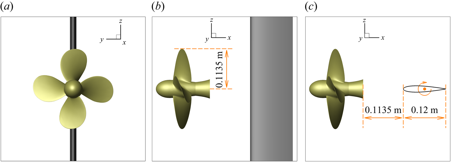
Figure 1. Front, side and top views of the geometry.
The propeller is the INSEAN E779A model, that has been the subject of many experimental and numerical studies in the literature (Di Felice et al. Reference Di Felice, Di Florio, Felli and Romano2004; Salvatore et al. Reference Salvatore, Pereira, Felli, Calcagni and Di Felice2006; Felli et al. Reference Felli, Camussi and Di Felice2011; Muscari et al. Reference Muscari, Di Mascio and Verzicco2013; Di Mascio et al. Reference Di Mascio, Muscari and Dubbioso2014). It is a four blade, fixed-pitch, right-handed propeller characterized by a nominally constant pitch distribution and a very low skew. Its main geometrical features are reported in table 1. The foil has a standard NACA 0015 profile with a chord  $c=0.12\ \textrm {m}$. The distance between the bottom face of the hub of the propeller and the leading edge of the foil is $d=0.1135\ \textrm {m}$, equal to the radius of the propeller. In general, the clearance of the rudder from the propeller is selected both to guarantee hydrodynamic efficiency (drag reduction, directional stability or manoeuvring) and mitigation of vibratory loads induced by pressure pulses associated with blade passage. The clearance can have different ranges for single screw ( $0.3 < x/D < 0.6$) and twin screw configurations ( $0.4< x/D<0.8$) due to their particular shape at the stern (Molland & Turnock Reference Molland and Turnock2007). Therefore, the selected value is a plausible trade-off to generalize for these two ship typologies. Moreover, this value has been also used in experiments (Miozzi & Costantini Reference Miozzi and Costantini2021) and numerical simulations (Muscari et al. Reference Muscari, Dubbioso and Di Mascio2017a). In the spanwise direction, the foil extends to the boundary of the numerical domain so that its tip vortices do not interfere with the slipstream of the propeller.
Table 1. Propeller parameters.

Two angles of attack of the foil have been considered:  $0^{\circ }$ and $4^{\circ }$. For the latter case, the foil has been rotated around the vertical axis passing through its midchord point.
4. Numerical simulation set-up
In the numerical simulations, the rotational speed of the propeller has been set to  $n = 17$ r.p.s. The inflow velocity is $U_\infty = 3.4$ m s $^{-1}$ so that the advance coefficient is $J = U_\infty / n D = 0.88$.
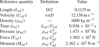
All quantities have been cast in non-dimensional form by using as reference values the radius of the propeller ( $L_{ref} = 0.1135$ m), the velocity of the tips of the blades ( $U_{ref} = n{\rm \pi} D \simeq 12.14$ m s $^{-1}$) and the density of fluid ( $\rho _{ref}= 1000$ kg m $^{-3}$). Other reference quantities are defined consistently with the principal ones, and are reported in table 2 in order to ease the conversion between non-dimensional values (used in most of following figures) and dimensional ones. Furthermore, assuming a kinematic viscosity of the water $\nu = 1.139\times 10^{-6}$ m $^{2}$ s $^{-1}$, the Reynolds number is ${Re} = U_{ref}L_{ref} / \nu = 1.211\times 10^{6}$.
Table 2. Reference values used for casting quantities in non-dimensional form.
With these choices, the non-dimensional period of revolution of the propeller is  $T = 2{\rm \pi}$.
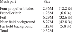
As said above, the computational mesh is made up of structured, overlapping blocks. In figure 2 a sketch of the blocks around the bodies and in near-field background is shown. The simulation of the flow is wall-resolved and the total number of cells is approximately  $1.9\times 10^{7}$, distributed according to table 3.
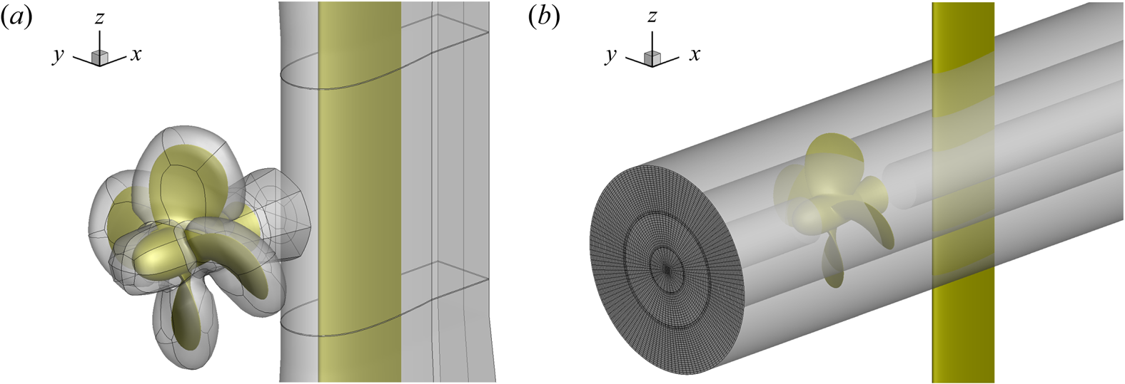
Figure 2. Sketch of the grid blocks around propeller and foil (a) and in the near-field background (b).
Table 3. Distribution of computational cells.
Finally, the time step corresponds to a rotation of one degree for the propeller, which is  $dt = 2{\rm \pi} / 360 \simeq 0.1745\times 10^{-1}$.
5. Structural model
The modelling and simulation of the rudder dynamical response to hydrodynamical forces were carried out through the commercial finite element (FE) code Comsol Multiphysics. In the following, a brief description of the mathematical model, of the structural properties of the rudder and of the surface mesh used for structural computations, obviously different from that used for fluid dynamics simulations, is given.
5.1. Governing equations
The basic governing equations of FSI are expressed in discrete form as follows:
 \begin{equation} (\boldsymbol{\mathsf{M}}+\boldsymbol{\mathsf{M}}_{f})\ddot{\boldsymbol{u}} + (\boldsymbol{\mathsf{C}}+\boldsymbol{\mathsf{C}}_{f})\dot{\boldsymbol{u}} + (\boldsymbol{\mathsf{K}}+\boldsymbol{\mathsf{K}}_f)\boldsymbol{u} = \boldsymbol{F}_{\boldsymbol{r}},\end{equation}
where  $\ddot {\boldsymbol{u}}$, $\dot {\boldsymbol{u}}$, $\boldsymbol{u}$ denote the acceleration, velocity and displacement vectors of the nodes of the structural model, respectively. The mass, damping and stiffness matrices of the structure, $\boldsymbol{\mathsf{M}},\boldsymbol{\mathsf{C}},\boldsymbol{\mathsf{K}}$, are defined as
 \begin{equation} \boldsymbol{\mathsf{M}}=\int_{V}{\rho_s\boldsymbol{\mathsf{N}}^{\rm T}\boldsymbol{\mathsf{N}}\,{{\rm d}}V},\quad \boldsymbol{\mathsf{C}}=\int_{V}{c\boldsymbol{\mathsf{N}}^{\rm T}\boldsymbol{\mathsf{N}}\,{{\rm d}}V},\quad \boldsymbol{\mathsf{K}}=\int_{V}{\boldsymbol{\mathsf{B}}^{\rm T}\boldsymbol{\mathsf{D}}\boldsymbol{\mathsf{B}}\,{{\rm d}}V}, \end{equation}
where  $\boldsymbol{\mathsf{N}}$ is the displacement interpolation matrix, $\boldsymbol{\mathsf{B}}=\partial N$ the strain-displacement matrix and $\boldsymbol{\mathsf{D}}$ the material constitutive matrix. The variables $\rho _s$ and $c$ denote the mass density and damping of the structure, respectively. Here $\boldsymbol{\mathsf{M}}_{f}$, $\boldsymbol{\mathsf{C}}_{f}$, $\boldsymbol{\mathsf{K}}_{f}$ are the hydrodynamic added mass, damping and stiffness matrices due to the FSI. Detailed formulation of these matrix identities can be found in Harwood et al. (Reference Harwood, Felli, Falchi, Garg, Ceccio and Young2020). The external load $\boldsymbol{F}_{\boldsymbol{r}}$ contains only hydrodynamical force $\boldsymbol{F}_{\boldsymbol{r}} = \int _{S}{\boldsymbol{\mathsf{N}}^\textrm {T}\boldsymbol{P}\,{\textrm {d}}S}$, as the weight and buoyancy terms are considerably small in relation to the fluid dynamic load on the rudder. The pressure load $\boldsymbol{P}$ acting on the rudder is obtained from CFD simulation and inserted in the FE model as distributed face load. In order to use the hydrodynamic load predicted by the CFD in the term $\boldsymbol{P}$, interpolation is required, since fluid and structure grids are generally non-matching.
Equation (5.1) can be solved by using two different approaches: a direct integration method; or a modal superposition, where a model reduction is obtained using the eigenvalue problem to construct a basis for the system. The choice for one method or the other is determined only by their numerical effectiveness. In fact, the solutions obtained using either procedure are identical within the numerical errors of the time integration schemes used (Bathe Reference Bathe2014).
In the present case, the frequency band of the excitation is limited to a narrow range between a few Hertz and a few hundreds of Hertz and, hence, only few eigenfrequencies should be sufficient to prevent modal truncation errors. For this reason, the modal superposition approach would be faster than the direct integration of the system equation. However, the adopted FE code accepts only analytical time-dependent loads and, moreover, all the loads must have the same dependency on the time (Comsol Reference Comsol2020). These limitations make the modal superposition approach unpractical, and direct integration is used in this work.
5.2. Structural model and computational set-up
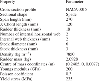
The analysed rudder assembly consists of the rudder blade, with two horizontal stiffeners, located at 33 % and 66 % of its length, respectively, and the rudder stock, which is located at 30 % of the chord length from the leading edge (see figure 3). The material of the rudder is isotropic and the mechanical properties together with the main rudder geometric characteristics are reported in table 4. The stock dimensions as well as the rudder thickness have been chosen taking into account the guidelines rules suggested by the Det Norske Veritas classification society (DNV-GL 2015).
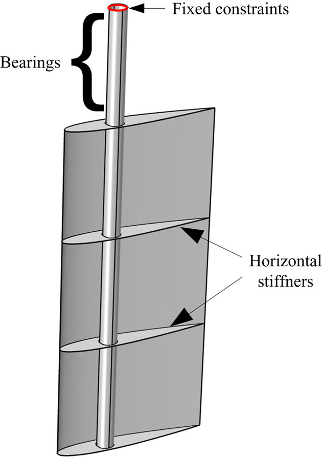
Figure 3. Structural model of the rudder and its boundary conditions.
Table 4. Structural characteristics of the rudder.
The boundary conditions that have been implemented in the structural simulation replicate the realistic arrangement of the rudder, see figure 3. Specifically, the topmost nodes of the stock are assumed to be rigidly fixed, with all the displacement and rotational degrees of freedoms restrained. The nodes that coincide with the region of the bearings within the steering gear are fixed against displacements but they are free to rotate around the stock axis.
An acoustic domain is used to simulate the water, and non-reflecting boundary conditions are applied at the boundaries of the acoustic fluid domain to approximate an infinite space. Preliminary simulations were performed using a cylindrical water domain of increasing dimension, in order to prevent boundary condition influences on the structural response.
5.3. Structural mesh
In figure 4 the FE model on the rudder embedded in the acoustic domain is depicted. The rudder, the internal stiffeners and the stock have been modelled with second-order (quadratic) shell elements, each one with its own thickness. The formulation used in the simulation is of Mindlin–Reissener type (Bathe & Dvorkin Reference Bathe and Dvorkin1985) in order to account for the transverse shear deformation. The rudder and the stock are discretized through quadrilateral elements equal to 1800 and 912 elements, whereas internal web and top and bottom plates are discretized using 336 and 376 triangular elements, respectively. This mesh size was obtained by a preliminary sensitivity analysis performed by calculating rudder displacements and stresses with different mesh sizes to ensure that the results of the structural analysis are not influenced by the density of the mesh. The mesh was progressively refined until any further cell size reduction did not affect remarkably the calculated displacements and stresses.

Figure 4. The FE mesh of the rudder (green) embedded in the acoustic domain (grey).
At their common boundaries, the CFD mesh is significantly finer than the structural one, therefore an interpolation of the pressure data from CFD to FEM meshes is required. Pressure data at CFD mesh nodes are transferred to the structural mesh nodes using bilinear interpolation. A comparison of the pressure distribution obtained from CFD and the interpolated one on the structural grid is presented in figure 5 in terms of contour lines on the wall of the rudder and shows a very good agreement. The reliability of the interpolation method used to transfer the pressure data is further highlighted in figure 5, where the absolute value of interpolated pressure load received by the structure at a generic point on the pressure side is almost overlapped with the value of the CFD pressure data in the nearest CFD grid point.
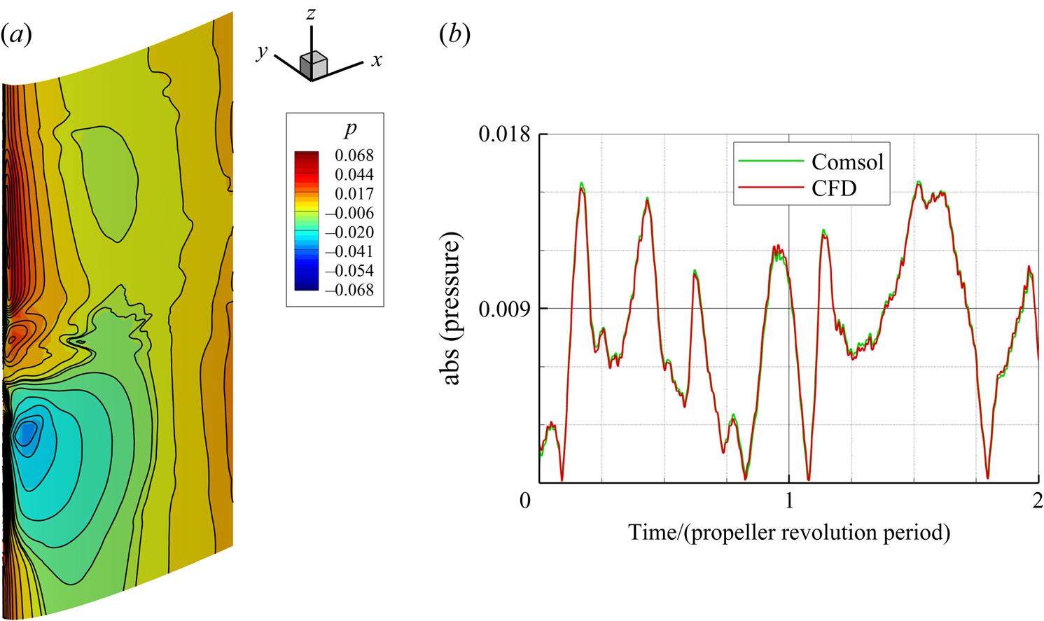
Figure 5. Comparison of the pressure predicted by CFD and its interpolation on the structural grid. (a) Instantaneous pressure distribution on the rudder surface, CFD data are represented using contour lines, while data interpolated on the structural grid are represented in solid colours. (b) Time history of the pressure load at a generic point on the pressure side: CFD data (red) versus data interpolated by FEM code (green).
The acoustic domain used to simulate the water around the rudder is meshed using  $1.4\times 10^{5}$ tetrahedral elements. The acoustic elements on the rudder surface have the same nodes of the structural domain, and become coarser far from the surface.
The time step used for the structural analysis is the same as the CFD simulation, which is sufficiently small to achieve a convergence of all residuals to the order of  $10^{-5}$.
The generalized alpha method (Hulbert & Chung Reference Hulbert and Chung1996) is implemented in order to solve the transient analysis. This is a generalization of the Newmark method, widely used for structural dynamics problems, which is an implicit time-stepping scheme of second-order accuracy. A time period equal to eight propeller revolutions is covered and, since the time step used in the hydrodynamic simulations was equivalent to  $1^{\circ }$ rotation of the propeller, this corresponds to 2880 temporal solutions. Hence, the resultant sampling frequency satisfies the Nyquist–Shannon criterion up to 3 kHz.
6. Results
6.1. Flow field description
Before quantitatively analysing the loads on the rudder and the corresponding structural response, a brief description of the flow dynamics past the propeller and around the foil is given in this section.
In general, the sections of the rudder experience an incidence angle that changes along the span due to the combination of the deflection angle  $\delta$ of the whole rudder and the swirl velocity induced by the propeller,
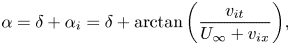 \begin{equation} \alpha = \delta + \alpha_{i} = \delta + \arctan{ \left(\frac{v_{it}}{U_\infty + v_{ix} } \right)}, \end{equation}
where  $v_{ix}$ and $v_{it}$ are the axial and tangential components of the velocity induced by the propeller in the slipstream. The orientation of $v_{it}$ is concordant to blade rotation. Therefore, it is positively oriented at $z>0$ and amplifies the static incidence $\delta$, vice versa for $z<0$ (see figure 6). It is evident that the antisymmetric flow established for the rudder in neutral condition is lost for the case at incidence. Accordingly, the domain of the rudder is divided into four quadrants, that, for the deflected case, experience each different flow conditions. In the following, we will indicate as the first quadrant the upward part of the back of the rudder, $y>0, z>0$. The remaining three quadrants are defined consecutively with the rotation of the blade.
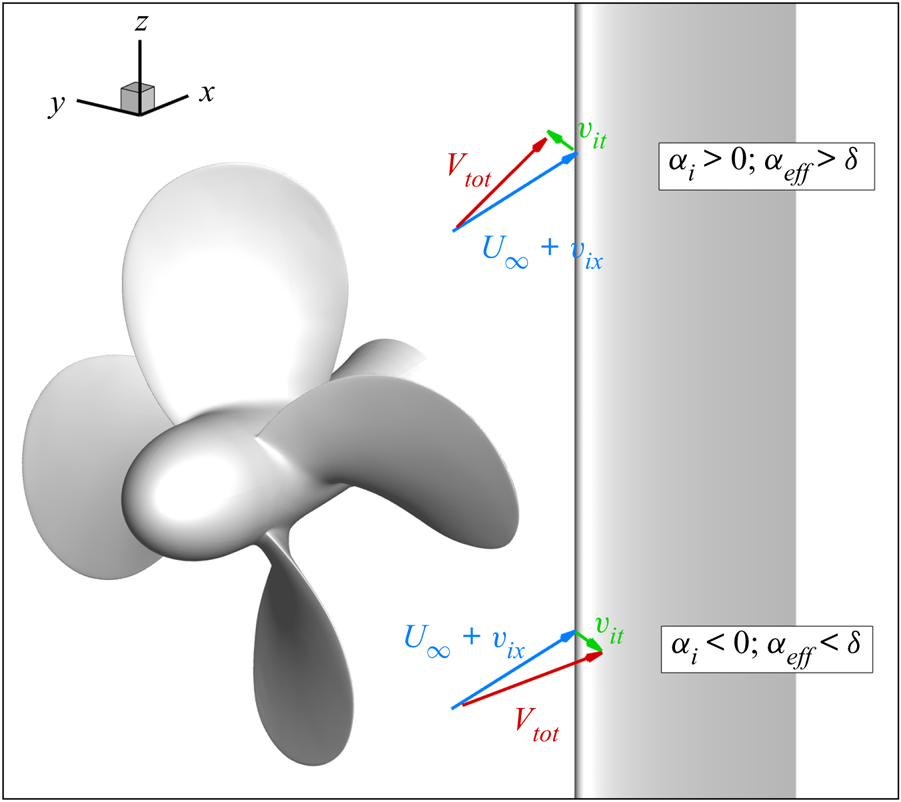
Figure 6. Nominal velocities induced by the propeller on the rudder. The opposite orientation of the tangential component  $v_{it}$ determines increments of incidence of opposite sign on the upper and lower half of the rudder.
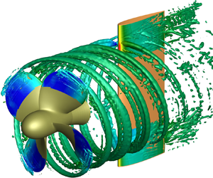
The flow field that characterizes the propeller–rudder interaction is visualized in figures 8–11 for the rudder in neutral position (figures 8a,c, 10a,c and 11a,c) and at incidence (figures 8b,d, 10b,d and 11b,d). The vortical structures, identified by the  $\lambda _2$ criterion (Jeong & Hussain Reference Jeong and Hussain1995) in figure 8, highlight the heterogeneous nature of the wake field of the propeller that interacts with the rudder. On one side, the structures released at the tip of the blades are coherent and impinge intermittently the wall at the BPF. On the other hand, from the hub of the propeller a markedly stronger system, composed by elements at different length scales, impinges almost continuously the rudder. In this case, the structure of the hub vortex is more complicated with respect to that reported in Muscari et al. (Reference Muscari, Dubbioso and Di Mascio2017a). In fact, the flow is completely separated past the hub as a consequence of its bluff geometry. Swirling flow and low pressure provoke a strong recirculation and reorganization of vorticity from the blade root vortices and the boundary layer of the hub into smaller structures. Moreover, this mechanism breaks the link between the hub vortex and the blade vortex sheet and, in conjunction with the bluff body flow, destabilizes the hub vortex.
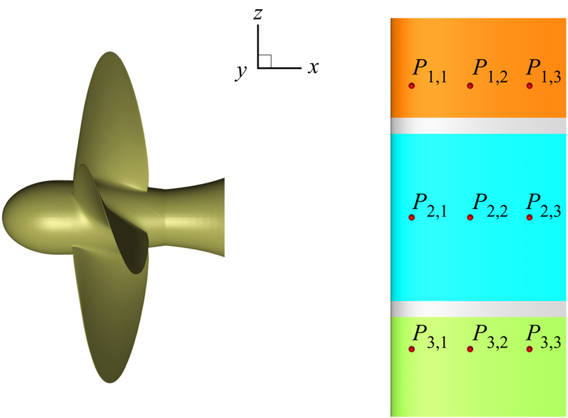
Figure 7. Layout of probes and identification of hub load region (cyan), tip region at top (orange) and tip region at bottom (green).
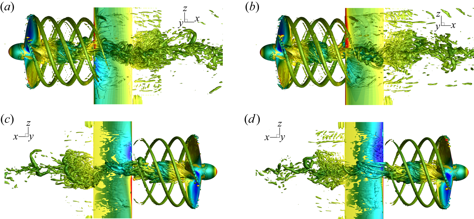
Figure 8. Vortex field identified by  $\lambda _2$ criterion, isosurface coloured with pressure: (a,c) $\delta =0^{\circ }$; (b,d) $\delta =4^{\circ }$. (a,b) View of the pressure side of the foil, (c,d) view of the suction side.


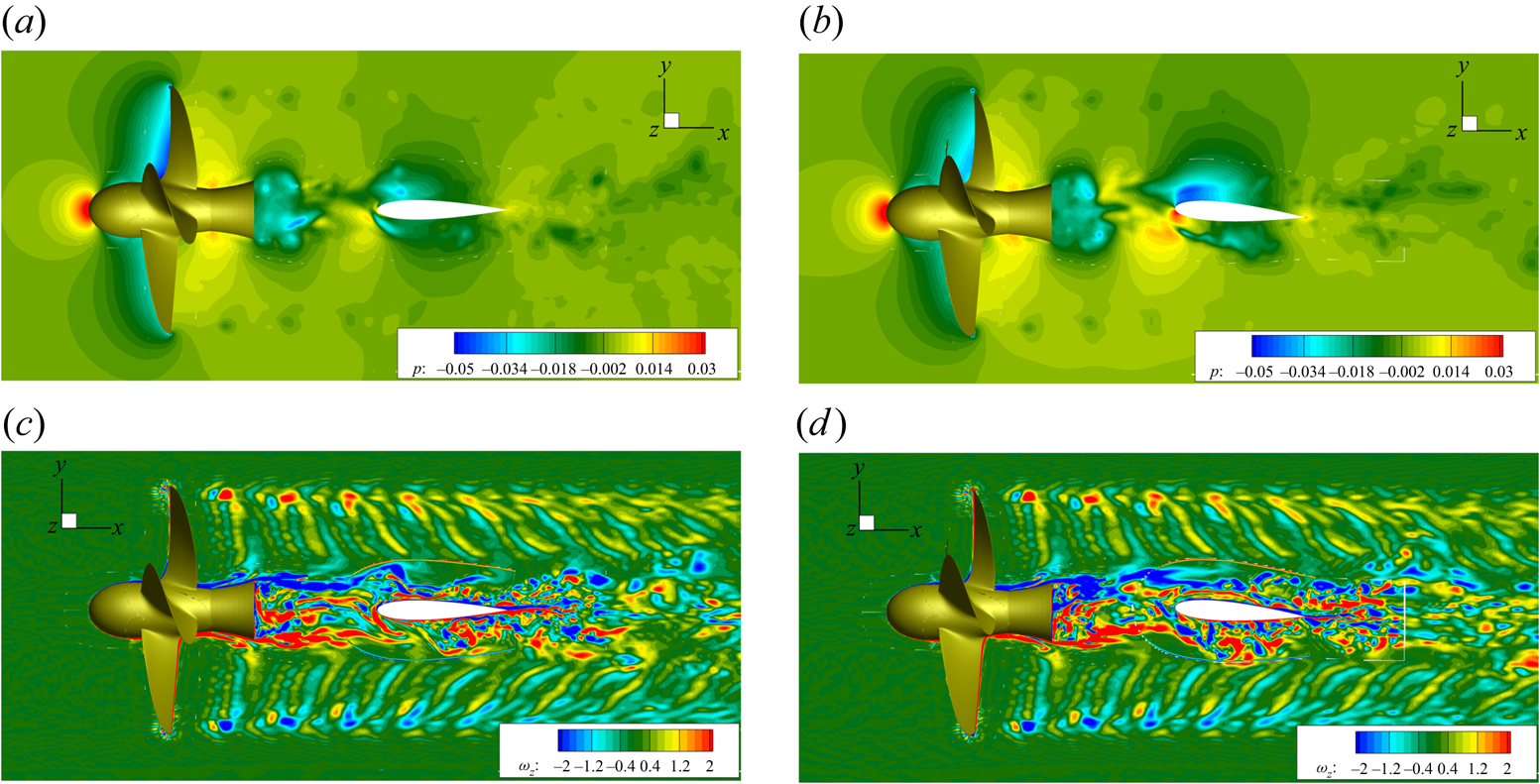
Figure 10. Instantaneous flow quantities on the horizontal plane at  $z=0$: (a,c) $\delta =0^{\circ }$; (b,d) $\delta =4^{\circ }$. (a,b) Pressure distribution, (c,d) vertical component of vorticity $\omega _z$.

Figure 11. Instantaneous flow quantities on the horizontal plane at  $z=0.7$: (a,c) $\delta =0^{\circ }$, (b,d) $\delta =4^{\circ }$. (a,b) Pressure distribution, (c,d) vertical component of vorticity $\omega _z$.
In order to stress the different interaction of the hub and tip vortices with the rudder, the pressure and the vertical component of vorticity  $\omega _z$ are extracted at a generic instant on the horizontal planes sketched in figure 9, and the resulting fields are shown in figures 10 and 11.
During the convection phase, the interaction of the tip vortex with the wall is substantially softer with respect to the hub vortex. The vortical structures, represented in terms of the vertical component of vorticity  $\omega _z$, highlight that the morphology of the tip and blade vortex sheet is unchanged far from the wall, while it is gradually weakened during the downstream convection. On the other hand, the hub vortex interacts more profoundly with the boundary layer of the rudder, and gives onset to the formation of larger structures detached past the trailing edge. It has to be noted that at $\delta =4^{\circ }$ the asymmetry between the portion of hub vortex on the back and face of the rudder is more evident in contrast to the flow induced by tip vortices. Moreover, from the vorticity maps, it can be observed that the blade vortex sheet is detached from the hub vortex before the interaction with the rudder.
A more quantitative inspection of the propeller–rudder interaction is described by the harmonic analysis at some probes located in the back and face of the rudder, representative of the tip and hub vortex regions, see figure 7. The probes are located at 10 %, 50 % and 80 % of the chord from the leading edge, and at height  $z = \pm 0.9$ (tip zone) and $z = 0$ (hub zone). In the legend of the figures, probes on the suction and pressure sides of the rudder are referred to as B (back) and F (face), respectively. In figures 12 and 13 the harmonic analyses of wall pressure at neutral position and $\delta =4^{\circ }$ are presented for both face and back sides. Due to the almost symmetric conditions, the harmonic analysis for the rudder at neutral positions (figure 12) refers only to the probes on the face of the body. In the figures, red and black lines refer to the probes located close the leading edge and trailing edge, respectively. Moreover, symbols are associated with the SF (17 Hz), first BPF (68 Hz) and second BPF (136 Hz). In the tip regions the signal is characterized by tones at multiples of the BPF, which are one order of magnitude greater than the component associated with the SF. Moving to the trailing edge, tones higher than the first BPF drops as a consequence of the interaction with the boundary of the rudder and gradual weakening of the structure. It is interesting to observe the wide bump centred about the frequency at 110 Hz (in-between the first and second BPF), that is conserved up to the trailing edge and is stronger on the pressure side of the rudder. This component can be ascribed to nonlinear effects associated with vorticity reorganization during the interaction between tip and blade vortex sheet with the boundary layer of the rudder in conjunction with the long wave instability of the tip vortex, caused by travelling pressure waves after the collision with the wall. On the other hand, in the region of the hub vortex the signal is broadband due to the strong vorticity mixing and morphology evolution associated with the interaction with the boundary layer of the rudder. The signal of the probe close to the leading edge is dominated by the tone at the SF (ascribed to the collision of the structure with the wall), which is stronger with respect to the pressure fluctuations induced by the collision of the tip vortices.
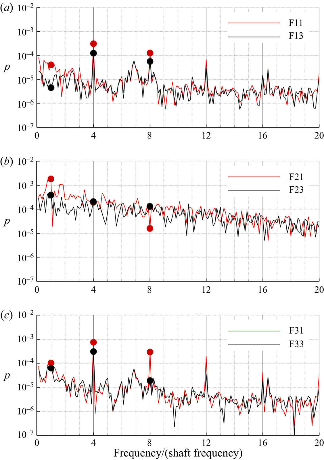
Figure 12. Fast Fourier transform (FFT) of wall pressure  $\delta =0^{\circ }$. Red lines refer to the probes located close the leading edge, while black lines refer to the probes near to the trailing edge. Symbols are associated with the SF (17 Hz), first BPF (68 Hz) and second BPF (136 Hz).

Figure 13. The FFT of wall pressure  $\delta =4^{\circ }$. Probes on the suction and pressure sides of the rudder are referred to with B (back) and F (face), respectively. Panels (a,c,e) are the third–fourth quadrant and (b,d,f) are the first–second quadrant.
In order to unravel the structural response of the rudder, the forces and moments as well as their distribution are shown in figures 14–16. Consistently with the structural analysis, the loads are split into mean and fluctuating components, that are associated with the static and dynamic motions of the rudder, respectively. In more detail, figure 14 shows the spanwise distribution of the side force  $F_Y$ (black) and vertical moment $M_Z$ (red) for $\delta =0^{\circ }$ (solid) and $\delta =4^{\circ }$ (dashed). For both angles, the loads have the same trends, because at these incidences there is no flow separation. In the neutral condition, the loads are antisymmetric with respect to the origin, because the hydrodynamic incidence is entirely given by the velocity field induced by the propeller wake (see figure 6 and (6.1)). On the other hand, at $\delta =4^{\circ }$ the velocity induced by the propeller causes the upper half of the rudder to be more loaded than the lower side. The time histories of the side force and torque are reported in figure 15. The loads refer to the total component and the individual ones for the tip and hub vortices, referred to the regions identified in figure 7. In the neutral position (left-hand subpanel), $F_Y$ and $M_Z$ are stronger and oppositely signed for the top and bottom regions due to the opposite inflow velocity induced by the propeller. On the other hand, the loads in the hub region are characterized by a small mean value and strong fluctuations, whose amplitude are an order of magnitude higher with respect to the fluctuating components of the loads at the tips. At $\delta =4^{\circ }$ (right-hand subpanel), the relative contribution from the three regions of the rudder changes: the hub vortex zone develops the stronger side force and rudder torque with respect to the tips. Consistent with the spanwise distribution in figure 14, the tip region at the bottom is weakly loaded due to the concurrent contribution between rudder deflection and propeller-induced velocity.

Figure 14. Distribution of lift  $F_{Y}$ and torque $M_{Z}$ on the rudder: solid, $0^{\circ }$; dashed, $4^{\circ }$.

Figure 15. Time histories of lift ( $F_{Y}$) and torque ( $M_{Z}$) for split and total loads: tip region at bottom (red); tip region at top (blue); hub (green); total (grey). Here (a,c) $\delta =0^{\circ }$; (b,d) $\delta =4^{\circ }$.

Figure 16. The FFT of  $F_{Y}$ of split and total loads: tip region at bottom (red); tip region at top (blue); hub (green); total (grey). Here (a,c) $\delta =0^{\circ }$; (b,d) $\delta =4^{\circ }$.
Figure 16 shows the harmonic content of the resultant and split contributions of  $F_Y$ for the neutral and deflected rudder conditions, respectively. The load fluctuations are mainly ascribed to the dynamics of the hub vortex and are associated with both tonal and broadband frequencies. The most energetic frequencies of the side force are in the low-frequency range, namely up to the first BPF. In more detail, the split contribution shows that the hub vortex provides a dominant contribution at the SF and in the whole broadband range. On the other hand, the contribution from the tip region is tonal, the spectra featuring dominant peaks at multiples of the BPF (68 Hz). However, the dynamics of the hub vortex affects the load in the tip region in the lowest frequency range, since the peak at the SF and broadband contribution is more than one order of magnitude in this range with respect to the remaining part of the spectrum. This aspect can be associated with strong vorticity distribution and reorganization in the propeller slipstream associated with the meandering of the hub vortex. A further contribution that probably takes place in the early phases of the interaction can be associated with the blade sheet: being a bridge between hub and tip structures, it can somehow transmits the fluctuations from one vortex structure to the other and vice versa, as conjectured in Muscari et al. (Reference Muscari, Dubbioso and Di Mascio2017a) in relation to the dynamics of the hub vortex during the collision phase with the wall. It is interesting to observe that when the rudder is deflected, the contribution at SF is dominant as a consequence of the oblique impingement of the structure that yields a stronger stagnation area on the wall. The relative contributions of the hub and tip region to the fluctuation characteristics of $M_Z$ are consistent with those of the side force and, hence, are not reported for conciseness.
6.2. Dry and wet natural frequencies
The modal analysis of the rudder in dry and wet conditions is performed in order to assess modes and associated frequencies. The damping matrices in (5.1) are neglected in the current analysis. Therefore, the eigenvalue problem to solve is
 \begin{equation} (-\omega^{2} (\boldsymbol{\mathsf{M}}+\boldsymbol{\mathsf{M}}_{f}) + \boldsymbol{\mathsf{K}}+\boldsymbol{\mathsf{K}}_{f})\boldsymbol{\varPhi}=0, \end{equation}
where  $\omega$ denotes the circular frequency and $\boldsymbol{\varPhi}$ the eigenmodes. The commercial FE Comsol Multiphysics software was used to solve (6.2). The solver uses the ARPACK routines for large-scale eigenvalue problems, which is based on a variant of the Arnoldi algorithm (Lehoucq, Sorensen & Yang Reference Lehoucq, Sorensen and Yang1998). This algorithm is particularly computationally cost effective with large sparse systems. The vibration characteristics of the rudder in water change substantially with respect to the dry condition, mainly due to the added mass effect in water (Blevins Reference Blevins2001).
In table 5 the first four natural frequencies are reported, and their mode shape is depicted in figure 17. Since there is no difference between the first four dry and wet mode shapes, only the last ones are visualized.
Table 5. Dry and wet natural frequencies (in Hertz) of the rudder.


Figure 17. Mode shapes of the plate: (a) mode 1 (99.73 Hz); (b) mode 2 (142.15 Hz); (c) mode 3 (523.33 Hz); (d) mode 4 (694.16 Hz).
Due to the added mass effect of the water, the in-water natural frequencies of the rudder are lower than the corresponding in-air ones. This is consistent with findings from previous numerical and experimental works (Fahy Reference Fahy1985; Ciappi et al. Reference Ciappi, Magionesi, De Rosa and Franco2009). From the analysis of the figures, it is evident that the first mode is primarily flapwise bending, while the second is an edgewise bending mode. The third one is a torsional mode, while the fourth a second-order flapwise mode. Since the flapwise direction of motion is accompanied by a larger volume of displaced water, which leads to higher fluid inertial resistance, than the edgewise direction, the reduction of in-water natural frequencies with respect to dry natural frequencies is significantly higher for the flapwise condition than the edgewise one. Therefore, the added mass is much different in those two cases. Moreover, the effect of the surrounding fluid is different for bending-dominated versus twisting-dominated modes. In figure 18, the ratio between the natural frequency in dry and wet conditions is reported.

Figure 18. Variation of the ratio between wet and natural frequencies for the first nine modes.
6.3. Structural response
The rudder structural response to hydrodynamic load generated by a propeller is investigated here in terms of deformations and stresses.
To gain a deeper insight on the effects of the interaction with the propeller wake, three different loading conditions are considered. In particular, in addition to the hydrodynamic load induced by the complete propeller wake system (global load condition), the split contributions of the wake in the hub and tip zones (as defined in figure 7) are separately considered. For the sake of clarity, the split conditions are visualized in figure 19.
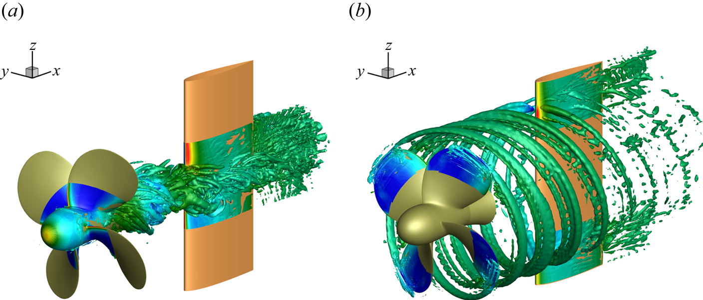
Figure 19. Partial loading conditions on rudder: (a) hub vortex load; (b) tip vortex load.
The three displacement components were monitored by 18 probes located on the rudder pressure and suction sides. For each side, three rows of probes along the rudder span were considered, corresponding to tip ( $z = \pm 0.9$) and hub ( $z = 0$) regions, each row consisting of three probes positioned at 10 %, 50 % and 80 % of the chord (see figure 7).
6.4. Angle of attack  $\delta = 4^{\circ }$

The time-averaged deformation of the rudder under the global load condition is depicted in figure 20. Since the rudder is lifting, the side force is the dominant load and thus the rudder is bent to the positive  $y$ direction. The time history of the rudder response, shown for the probe $\textrm {F}_{2,1}$ in figure 21, further highlights that the mean values and the maximum fluctuations in the $x$ (U) and $z$ directions (W) are almost one order of magnitude smaller compared with those in the $y$ direction (V).

Figure 20. Time-averaged rudder deformation, normalized with respect to the span, under global load condition,  $\delta =4^{\circ }$.
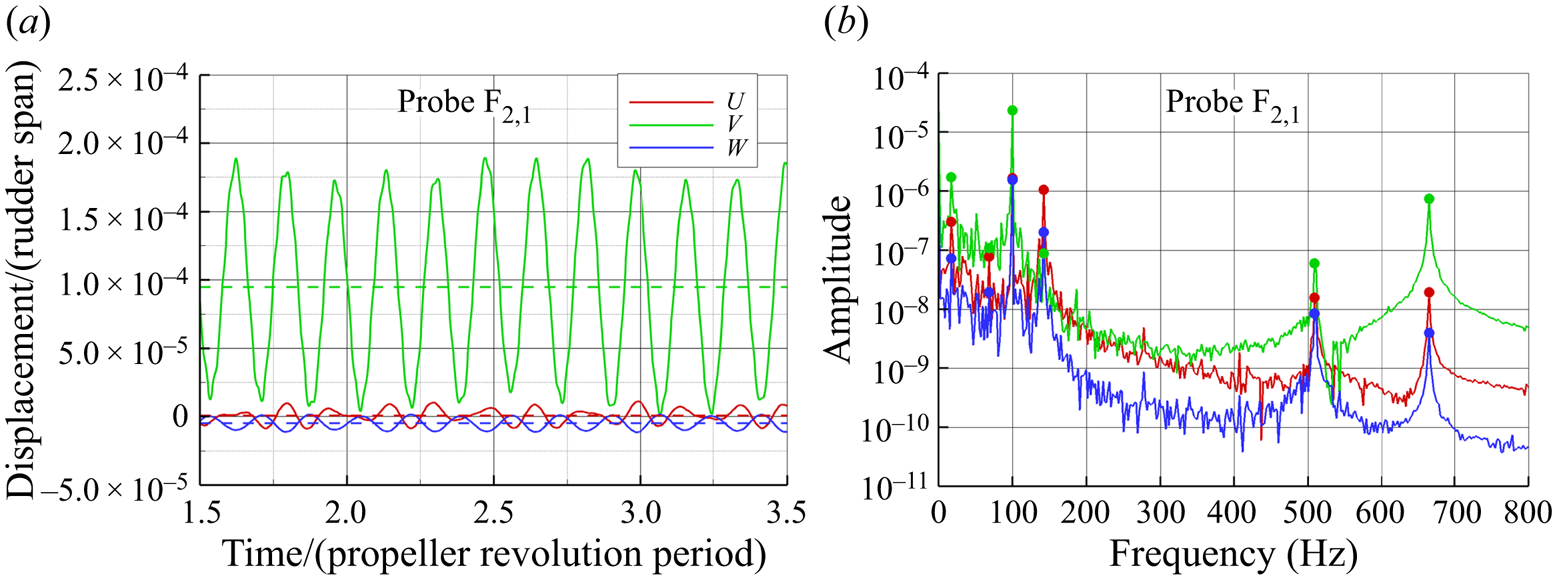
Figure 21. Time histories of the displacement components at probe  $\textrm {F}_{2,1}$ for (a) global loading condition and (b) corresponding Fourier transform, $\delta =4^{\circ }$.
The corresponding harmonic analysis by the FFT is shown in figure 21(b). The spectra of the displacement components are characterized by two frequency bands: a low-frequency band (below the first natural in-water frequency) with peaks associated with the hydrodynamic load (shaft and BPFs) and a midfrequency band characterized mainly by distinct resonance peaks of the rudder system with a strong modal character of the vibratory behaviour.
In the midfrequency range, the FFT spectrum of V component is characterized by three peaks corresponding to first flapwise, first torsional and second flapwise modes. The peak related with the first edgewise mode (142.15 Hz) is stronger for the U component by almost one order of magnitude with respect to V and W. At low frequency (figure 22a), below the first structural natural frequency (flapwise bending), the displacement spectra are dominated by the peak associated with the first SF (17 Hz). The peak corresponding to the first BPF at 68 Hz is evident only in the U and W components, instead. In the case of the V component, the harmonic associated with the second BPF (136 Hz) is more evident than the first, due to the proximity of a resonance condition with the first edgewise mode (142.15 Hz).
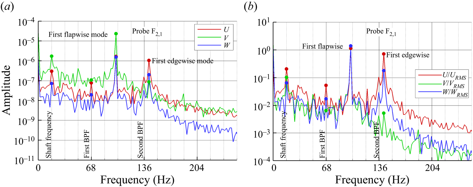
Figure 22. The FFT of  $\textrm {F}_{2,1}$ displacement components for global loading condition. $\delta =4^{\circ }$: (a) absolute components; (b) normalized components $U/U_{RMS}$, $V/V_{RMS}$, $W/W_{RMS}$.
An alternative perspective on the vibrational response is proposed in figure 22(b) considering the ratio of the displacements with respect to their correspondent root mean square (r.m.s.) values, i.e.  $\tilde {U}=U/U_{RMS}$, $\tilde {V}=V/V_{RMS}$, $\tilde {W}=W/W_{RMS}$. With respect to $\tilde {V}$, $\tilde {U}$ is enriched by a higher number of spectral components, not only related to the resonance condition near the second bending mode (edgewise), but also in the whole low-frequency range. In fact, the spectral content below the first natural frequency is generally higher along the $x$ direction with respect the $y$ one, with higher peaks at 17 and 68 Hz that are associated with the combination of low-frequency motion of the propeller slipstream (i.e. precession) and hub vortex. Moreover, the broadband bump between 30 and 45 Hz might be excited by the interaction of the hub vortex with the wall, which is characterized by vorticity redistribution with the boundary layer.
The three components of the displacement, measured at probes in the same column, are almost identical in the low-frequency range, while some differences are highlighted at higher frequencies. For example, in figure 23(a), the time history of V for the first probes near the leading edge ( $\textrm {F}_{1,1}, \textrm {F}_{2,1}, \textrm {F}_{3,1}$, see figure 7) is depicted. The mean and fluctuating motion of the probes is gradually amplified from top to bottom: obviously, $\textrm {F}_{1,1}$ is on a portion of the rudder that is constrained to the stock and, hence, is more rigid.

Figure 23. Displacement component V for the first column of probes near the leading edge ( $\textrm {F}_{1,1}, \textrm {F}_{2,1}, \textrm {F}_{3,1}$) for global loading condition, $\delta =4^{\circ }$: (a) time histories; (b) FFT of the normalized component $V/V_{RMS}$.
The correspondent FFT decomposition, shown in figure 23(b) in non-dimensional form, further highlights that the fluctuation of the bottom of the rudder ( $\textrm {F}_{3,1}$) is mainly associated with the first flapwise and first torsional bending frequencies. The part of the rudder nearest to the stock ( $\textrm {F}_{1,1}, \textrm {F}_{2,1}$) is characterized by a relatively higher content for frequencies higher than 500 Hz. Note, however, the absence of the peak in correspondence with the first torsional mode for $\textrm {F}_{1,1}$, which is consistent with the shape of this mode reported in figure 17.
By comparing the results measured by the probes on the pressure and suction side, no significant differences are evident in the frequency range of interest in the  $x$ and $y$ directions, whereas the W displacement is characterized by an opposite sign consistently with the prevailing lateral bending motion, as depicted in figure 24.
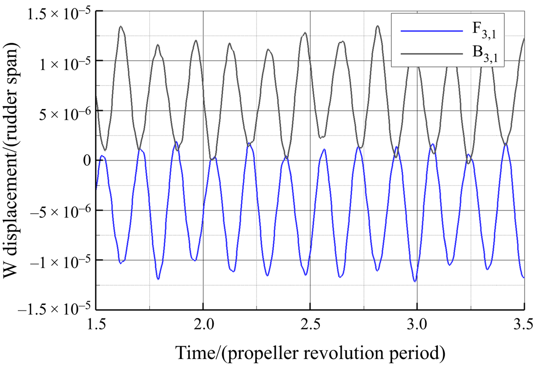
Figure 24. Comparison of the time histories of the displacement component W on pressure (blue) and suction sides (black) for global loading condition.  $\delta =4^{\circ }$.
In figure 25 the von Mises stresses for the global load condition are depicted. The higher stress concentration occurs in a narrow region that connects the rudder stock and the upper wet plate; the maximum value is equal to 72 MPa and it does not exceed the yield stress for the material selected, equal to 235 MPa.

Figure 25. Predicted von Mises stress distribution for global loading condition at a generic instant for  $\delta =4^{\circ }$.
In order to gain a deeper insight into the effects of the different vortical systems in the slipstream of the propeller on the rudder structural response, the separate contributions of the hub and tip vortex systems are analysed in contrast to the global one. When the rudder surface is loaded only by the vortical system shed by the hub or by the tip of the blade, the dynamical response of the elastic rudder is significantly different. The time history of the displacement along the  $y$ direction, due to the different loading conditions, for the probe $\textrm {F}_{2,1}$ and the associated harmonic analysis is depicted in figure 26. It is evident that the tip and hub vortical systems provide almost the same contribution to the V displacement component. In fact, the peak values of the harmonic corresponding to the first bending mode are identical. However, the frequency content in the low-frequency range is richer in the hub vortex region, due to the stronger vortex–body interactions. Instead, the contribution due to the vortical system shed by the tip excites, almost exclusively, the torsional mode of the rudder (523.33 Hz).

Figure 26. Time histories of the displacement component V monitored by probe  $\textrm {F}_{2,1}$ for (a) split and global loads and (b) corresponding results of FFT analysis, $\delta =4^{\circ }$.
The tip vortex provokes fluctuations of the edgewise component U similar to the hub vortex (see figure 27), although it is its action that determines the mean U displacement of the rudder, the mean contribution of the flow in the hub region being almost zero. Analogously to the V component, the tip vortex significantly affects the edgewise response via the torsional mode (523.33 Hz, figure 27b). In the low-frequency range, the hub vortex provides the strongest contribution, instead.

Figure 27. Time histories of the displacement component U monitored by probe  $\textrm {F}_{2,1}$ for (a) split and global loads and (b) corresponding results of FFT analysis, $\delta =4^{\circ }$.
In general, the comparison of the different vortical systems contributions to the spectral response measured on the rudder surface reveals that the structural excitation of U and V in the frequency range below 400 Hz due to the hub vortex excitation is higher than that due to the tip vortex. On the contrary, the tip vortex triggers stronger torsional vibrations.
Concerning the  $z$ direction, the contributions of the two different vortical systems are similar, see figure 28.
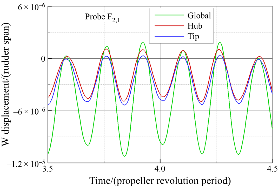
Figure 28. Time histories of the displacement component W for split and global loads monitored by probe  $\textrm {F}_{2,1}$, $\delta =4^{\circ }$.
Finally, in figure 29 the maximum von Mises stresses monitored for the three different loading conditions are depicted. These values are attained in the region of coupling between the rudder stock and the rudder blade, as highlighted in figure 25. It is evident that the tip and hub vortices contribute to the global von Mises stress equally.
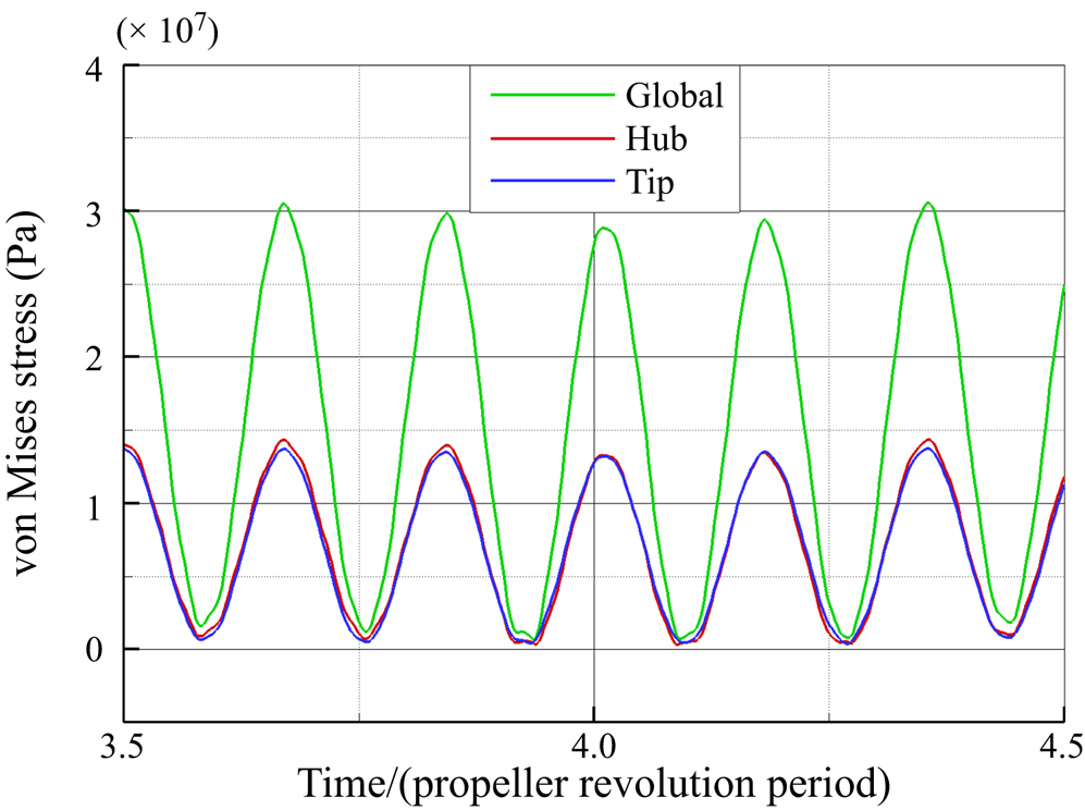
Figure 29. Maximum von Mises stress for split and global loads,  $\delta =4^{\circ }$.
6.5. Angle of attack $\delta = 0^{\circ }$ (rudder at neutral position)

The structural response of the rudder at  $\delta =0^{\circ }$ is significantly different with respect to the deflected condition $\delta =4^{\circ }$.
Figure 30, which represents the time averaged deformation, shows that the rudder bends towards the negative  $y$ direction, in opposition with the deflected condition (see figure 20). This is associated with the fact that at the unconstrained bottom of the rudder the lift is negative oriented according to the rotation of the propeller (see also figure 14). The different behaviour is also highlighted by the time history of the flapwise motion monitored on a representative probe on the rudder surface ( $\textrm {F}_{2,1}$) and the correspondent harmonic analysis shown in figure 31. The time history confirms the opposite value of the mean deflection and stresses that in the present case the amplitude of the fluctuation is in general smaller by approximately three times with respect to $\delta =4^{\circ }$.

Figure 30. Time-averaged rudder deformation, normalized with respect to the span, under global load condition,  $\delta =0^{\circ }$.

Figure 31. Comparison of time history of the displacement component V monitored by probe  $\textrm {F}_{2,1}$ for $\delta =4^{\circ }$ and $\delta =0^{\circ }$ (a) and corresponding results of FFT analysis (b).
The FFT of the non-dimensional displacement  $\tilde {V}$ (figure 32 and insert) further highlights that both the low-frequency content, related with hydrodynamical load, and the torsional vibrations are relatively higher at $\delta =0^{\circ }$. In comparison with the deflected case, the peak at the SF (17 Hz) is less evident; instead, a broad hump in the frequency response is present between 15 and 40 Hz. The peak corresponding to the second BPF (136 Hz) is clearly visible due to the closeness to the second structural resonance. Contrary to the $\delta =4^{\circ }$ case, it is also present, despite being not particularly pronounced, a peak at the first BPF (68 Hz). The neutral configuration is also characterized by a different distribution of energy at higher frequencies. In particular, the whole set of probes shows an increase of the dynamical response at a frequency close to the first torsional mode, and a reduction in the second flap mode response.

Figure 32. Comparison of the Fourier transform of the normalized displacement component  $V/V_{RMS}$ for $\textrm {F}_{2,1}$ at $\delta =4^{\circ }$ and $\delta =0^{\circ }$.
In contrast to  $\delta =4^{\circ }$, the displacement in the flow direction is dominated by the first edgewise mode (142 Hz), while the first flapwise mode is not excited, see figure 33(a). Moreover, at low frequencies, there is no peak corresponding to the shaft passing frequency (i.e. 17 Hz), whereas the peak corresponding to the first BPF is still visible. In the medium–high frequency range, the contribution ascribed to the torsional mode is stronger while the second flapwise mode is weaker.

Figure 33. Comparison of the FFT of the displacement component U (a) and W (b) for  $\textrm {F}_{2,1}$ at $\delta =4^{\circ }$ and $\delta =0^{\circ }$.
Concerning vertical displacement, shown in figure 33(b), the differences between the two tested conditions in the low-frequencies range are less evident, whereas, in the midrange, is confirmed a stronger torsional response and a strong reduction of the second flapwise mode.
Differences between the two conditions can be also evidenced by analysing the separate contribution of the tip and hub vortex systems. In fact, the comparison of the time history of the displacement in the  $y$ direction for the three different loading conditions shown in figure 34(a), stresses that the contribution from the tip vortex significantly overwhelms the one associated with the hub vortex, in contrast to their almost similar contribution at $\delta =4^{\circ }$. The harmonic analysis depicted in figure 34(b), shows that in the low-frequency range the fluctuations are correlated to the action of the hub vortex. In resonance conditions with the first flapwise and edgewise modes (i.e. 102 and 136 Hz, respectively), the displacement due to the tip vortex is significantly greater than that due to the hub vortex. It is also worth noticing that the response at frequency 136 Hz, close to the first edgewise mode, is mainly due to the tip load, and the same holds, even if with a smaller difference, for the first torsional mode.

Figure 34. Time histories of the displacement component V monitored by probe  $\textrm {F}_{2,1}$ for (a) split and global loads and (b) corresponding results of FFT analysis, $\delta =0^{\circ }$.
The effects of the tip and hub vortex systems on the edgewise component U are similar in terms of mean deflection and maximum fluctuation – see the time histories shown in figure 35(a). Similarly to the case at incidence, the tip vortex, in the hydrodynamic range of frequencies, excites the structure at the SF and the first BPF. It is interesting to notice the phenomenon of beating occurring when only the tip vortices are considered as a boundary load. In this kind of vibration, the amplitude increases and then diminishes in a regular pattern. This phenomenon occurs when the forcing frequency (in this case the second BPF) is close to the natural frequency of the system (first edgewise), as depicted in figure 35(b).

Figure 35. Time histories of the displacement component U monitored by probe  $\textrm {F}_{2,1}$ for (a) split and global loads and (b) corresponding results of FFT analysis, $\delta =0^{\circ }$.
The displacement in the  $z$ direction (W component) is mainly related to the tip vortex load for the whole set of probes, see figure 36(a). Analogously to the other two displacement components, the low-frequency response of the rudder is determined by the load exerted by the hub vortex (figure 36b). On the other hand, the peak of the fluctuation corresponding to the first flapwise mode is dominated by the action of the tip vortex system, its contribution being almost 66 % of the global displacement.

Figure 36. Time histories of the displacement component W monitored by probe  $\textrm {F}_{2,1}$ for (a) split and global loads and (b) corresponding results of FFT analysis, $\delta =0^{\circ }$.
Finally, the von Mises stresses evaluated for the three different loading conditions are presented in figure 37. With respect to  $\delta =4^{\circ }$, the maximum value of the von Mises stress is significantly lower and the contribution due to tip load is more than double that of the hub structure.
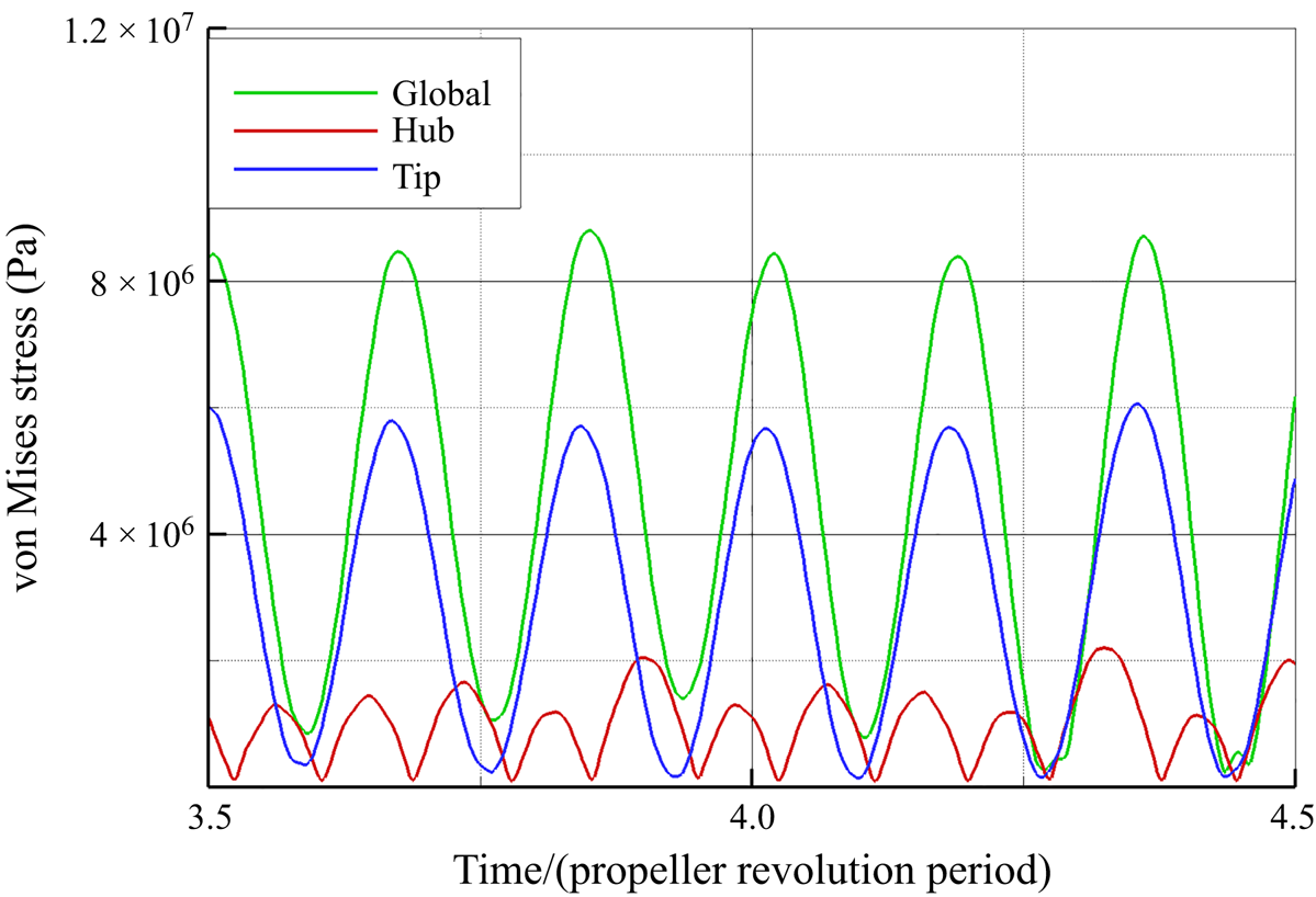
Figure 37. Maximum von Mises stress for different loading conditions,  $\delta =0^{\circ }$.
7. Summary and conclusions
In the present work, the FSI problem originating from the interaction of a rudder and the wake shed by an upstream propeller has been investigated by the one-way fluid–structure interaction paradigm. The test case consisted of the propeller INSEAN E779A and a rudder with rectangular plane area with sectional shape of a NACA 0015. The flow field and the resulting load on the rudder was assessed through DESs for operative conditions close to the design one: namely, the propeller was lightly loaded (advance coefficient at the design point  $J=0.88$) and the rudder was either at neutral position or at $4^{\circ }$ deflection. The flow and the structural response of the rudder are dominated by the interactions between the tip and hub vortex structures with the wall, that are imputable to both potential and viscous mechanisms. On this basis, the key contribution of this work was the analysis of the distinguished contribution of the two dominant vortical structures to the rudder response. In this regard, the flow simulation considered an infinite rudder in order to avoid the additional interaction of the tip vortex with that formed at the extremity of the rudder.
The analysis showed that, at both deflections, the structural response of the rudder is dominated by lateral and torsional deformations, while the edgewise deformations are negligible. In more detail, the vibrations of the rudder develop in a wide range of frequencies, the lower values being linked to the hydrodynamic interaction with the propeller wake and the higher values ascribed to its natural mode of vibration. In general, the response associated with the intrinsic mode of vibration of the structure is stronger with respect to those directly linked to the hydrodynamic interaction. Moreover, the behaviour in these two ranges resulted differently for the neutral and deflected configuration and the vibrations were weaker in the neutral condition. In particular, in the low-frequency range the dominant amplitudes were experienced at the SF, ascribed to the impingement of the hub vortex and precession motion of the whole propeller slipstream, and at the first BPF, ascribed to impingement of the tip vortices. In-between these two frequencies, the character of the spectrum is broadband, because of the manifold scales of the turbulent structures generated during the collision and travelling of the hub vortex with the wall.
The split analysis highlighted that the contribution of the tip vortex in the low-frequency range is weaker with respect to the hub vortex. Moreover, the propeller wake triggers, at a certain extent depending on the layout of the structure, its intrinsic mode of vibration. In this structural frequency regime, the rudder experiences fluctuations at frequencies associated with the first flapwise mode (100 Hz), to the edgewise mode (142 Hz), torsional mode (523 Hz) and second flapping mode (694 Hz) at both deflections. The edgewise mode is negligible with respect to the other modes. The torsional mode resulted in being stronger with respect to the second bending mode for the neutral deflection, and vice versa for the deflected condition. The vibration mode at 100 Hz, associated with the first flapping motion, was amplified at  $4^{\circ }$ with respect to $0^{\circ }$.
The analysis of the split contribution of the wake vortices highlighted that the lateral fluctuation at the first flapping frequency and first edgewise mode is more affected by the tip vortex in the neutral position, while at  $\delta =4^{\circ }$ the contribution of the two wake structures are similar. At highest frequencies for the deflected configuration, the tip and hub vortex exerts the dominant effect for the first torsional mode and second flapwise mode, respectively. Conversely, at $\delta =0^{\circ }$, these contributions are flipped. It is worthy of note that the fluctuation of the deformation caused by the hub vortex at $\delta =4^{\circ }$ is almost five times greater than that for the neutral position. As expected, the peak of the von Mises stress was concentrated in correspondence of the connection of the rudder stock and the top side of the rudder for both deflections. In the lightly loading condition investigated, the stress value was sufficiently far from the yield stress of the material.
The presented results are pertinent to the conditions tested, that, however, are representative of a relatively wide spectrum of ship operations concerning the canonical design condition in straight advance and manoeuvring at very small rudder angles for course keeping. The inclusion of a higher rudder angle of attack, heavier propeller loading and incidence angles representative of mild and tight manoeuvres are left to future investigations. In particular, time varying deflection of the rudder and free stream should be also tested to reproduce critical transients conditions that can be experienced during a realistic dynamic situation.
The proposed methodology is suitable for implementation in the optimization process of the rudder propeller system in the preliminary design stages. At the same time, the identification of the specific contribution of the tip and hub vortex can be helpful both to the design of the shape of the blade or development of advance blade pitch control strategies to weaken or alter the noise and vibratory signature of the ship.
Declaration of Interests
The authors report no conflict of interest.


 Open access