1. Introduction
Homogeneous isotropic turbulence is one of the most fundamental problems considered in turbulence research. The assumption of statistical homogeneity and isotropy simplifies the problem and allows the development of statistical theories. Turbulence far from a wall freely decays with time in the absence of an external force that injects energy into the flow. The theories for the decay of homogeneous isotropic turbulence were developed for the evolution of large-scale motions (Davidson Reference Davidson2004). Two types of isotropic turbulence are widely considered in turbulence theories: one is Saffman turbulence, whose three-dimensional energy spectrum is  $E(k\rightarrow 0)\sim k^2$ (Saffman Reference Saffman1967), where $k$ is a wavenumber; the other is Batchelor turbulence with $E(k\rightarrow 0)\sim k^4$ (Batchelor Reference Batchelor1953; Batchelor & Proudman Reference Batchelor and Proudman1956). Saffman turbulence and Batchelor turbulence have integral invariants, which do not change during the decay. These invariants are related to the conservation of linear momentum for Saffman turbulence and that of angular momentum for Batchelor turbulence. The invariant properties provide the constraint for root-mean-squared (r.m.s.) velocity fluctuations $U$ and a longitudinal integral length scale
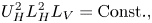
  $L$ during the decay, that is, $U^2L^3=\mathrm {Const}.$ for Saffman turbulence and $U^2L^5=\mathrm {Const}.$ for Batchelor turbulence. The invariant properties suggest that the turbulent kinetic energy $3U^2/2$ decays as $U^2\sim t^{-6/5}$ for Saffman turbulence and $U^2 \sim t^{-10/7}$ for Batchelor turbulence when the Reynolds number is large enough for the non-dimensional kinetic energy dissipation rate $C_\varepsilon =\varepsilon /(U^3/L)$ to be constant, where $\varepsilon$ is the kinetic energy dissipation rate.
These theories of decaying homogeneous isotropic turbulence have been assessed with experimental facilities of homogeneous isotropic turbulence. Nearly homogeneous isotropic turbulence is generated in wind tunnels by installing a grid at the entrance of test sections (Simmonsr & Salter Reference Simmonsr and Salter1934; Comte-Bellot & Corrsin Reference Comte-Bellot and Corrsin1966; Uberoi & Wallis Reference Uberoi and Wallis1967). Once turbulence is generated by the grid, it decays in the streamwise direction as the turbulence is advected by the mean flow. The theories for Saffman turbulence and Batchelor turbulence predict how turbulence evolves at large scales when the energy spectrum is given by  $E(k)\sim k^2$ or $k^4$. In realistic situations, turbulence is generated from laminar flows, which do not have the energy spectrum of turbulence. Therefore, the energy spectrum with $E(k)\sim k^2$ or $k^4$ can be formed when turbulence is generated. The theories do not clarify under what conditions turbulence with $E(k)\sim k^2$ or $k^4$ develops from a laminar flow. For this reason, it is not straightforward to determine whether grid turbulence belongs to Saffman turbulence, Batchelor turbulence or others. Experiments of grid turbulence often compare the evolutions of statistics with the theories of Saffman turbulence and Batchelor turbulence. In the theories, $U^2L^3$ and $U^2L^5$ are invariants of Saffman turbulence and Batchelor turbulence, respectively. Wind-tunnel experiments have confirmed that $U^2L^3$ hardly varies during the decay, indicating that the grid turbulence behaves similarly to Saffman turbulence (Krogstad & Davidson Reference Krogstad and Davidson2010; Kitamura et al. Reference Kitamura, Nagata, Sakai, Sasoh, Terashima, Saito and Harasaki2014). The decay exponent of the turbulent kinetic energy is generally close to that of Saffman turbulence (Krogstad & Davidson Reference Krogstad and Davidson2010; Kitamura et al. Reference Kitamura, Nagata, Sakai, Sasoh, Terashima, Saito and Harasaki2014; Sinhuber, Bodenschatz & Bewley Reference Sinhuber, Bodenschatz and Bewley2015; also see the papers cited in these studies). However, a discrepancy of the decay exponent from Saffman turbulence is also pointed out as the values of the exponent vary depending on experiments (Antonia et al. Reference Antonia, Lee, Djenidi, Lavoie and Danaila2013; Djenidi, Kamruzzaman & Antonia Reference Djenidi, Kamruzzaman and Antonia2015). The decay exponent is sensitive to the behaviour of two-point correlations at a large separation distance. Variations of the decay exponent can be caused by the effects of the finite size of wind tunnels because the walls can affect the long-range correlation of turbulence. An error in estimating the decay exponent may arise from the finite number of measurement points. In addition, the decay exponent is also sensitive to the turbulent Reynolds number $Re_\lambda$ when $Re_\lambda$ is not sufficiently large. The decay exponent may not be constant during the decay in previous experiments with moderate $Re_\lambda$ (Djenidi et al. Reference Djenidi, Kamruzzaman and Antonia2015). These issues in experiments of grid turbulence cause difficulty in concluding whether or not grid turbulence is Saffman turbulence.
Turbulence with stable density stratification is a common phenomenon observed in the environment, e.g. the atmospheric boundary layer (Mahrt Reference Mahrt1999) and the ocean mixing layer (Thorpe Reference Thorpe1978). The stable stratification can significantly alter the dynamics of turbulence because the stratification supports the propagation of internal gravity waves and suppresses vertical turbulent motions. Therefore, stably stratified turbulence has been extensively investigated by theories, laboratory experiments and numerical simulations for many years. As nearly homogeneous isotropic turbulence generated by a grid is useful to reveal the basic physics of turbulence, experiments have been conducted for grid turbulence in a stably stratified fluid. These experiments generate turbulence with a grid installed to wind tunnels or water channels (Itsweire, Helland & Van Atta Reference Itsweire, Helland and Van Atta1986; Lienhard & van Atta Reference Lienhard and van Atta1990; Yoon & Warhaft Reference Yoon and Warhaft1990; Huq & Britter Reference Huq and Britter1995; Komori & Nagata Reference Komori and Nagata1996) and a grid towed in a density-stratified water tank (Britter et al. Reference Britter, Hunt, Marsh and Snyder1983; Yap & Van Atta Reference Yap and Van Atta1993; Liu Reference Liu1995; Fincham, Maxworthy & Spedding Reference Fincham, Maxworthy and Spedding1996; Rehmann & Koseff Reference Rehmann and Koseff2004; Praud, Fincham & Sommeria Reference Praud, Fincham and Sommeria2005; Espa, Avallone & Cenedese Reference Espa, Avallone and Cenedese2018). Grid turbulence generated in a free stream of wind tunnels decays with the distance  $x$ from the grid. On the other hand, turbulence in towed-grid experiments decays with time $t$. However, these experiments can be compared by converting the distance $x$ in wind-tunnel experiments to time as $t=x/U_0$ with the mean velocity $U_0$.
The effects of stable stratification on the decay rate of turbulent kinetic energy have been reported in these experimental studies. However, the reported results are not conclusive: some experiments found that the decay rate is increased by the stratification while others found different effects, e.g. slower decay or no stratification influence on the decay rate. Wind-tunnel experiments of non-stratified grid turbulence have confirmed that the decay can be divided into three regimes: an initial, non-equilibrium decay period, where  $C_\varepsilon$ increases as turbulence decays; an equilibrium decay period with constant $C_\varepsilon$; and a final period of decay. The decay exponent close to Saffman turbulence was obtained for the equilibrium decay period in wind-tunnel experiments. When the turbulent Reynolds number is low, $C_\varepsilon$ increases toward the final period of decay. The decay of $U^2$ is described by ${\rm d} U^2/{\rm d} t=-C_{\varepsilon }(U^3/L)$, which is used together with $U^2L^3=\mathrm {Const}.$ or $U^2L^5=\mathrm {Const}.$ to derive $U^2\sim t^{n}$. The decay exponents of Saffman turbulence and Batchelor turbulence are obtained with the assumption of constant $C_\varepsilon$. If $C_\varepsilon$ increases with time, $n$ becomes larger than those derived for constant $C_\varepsilon$. Indeed, the decay exponent obtained for the near-grid region is larger than 1.2 of Saffman turbulence (Komori et al. Reference Komori, Nagata, Kanzaki and Murakami1993; Krogstad & Davidson Reference Krogstad and Davidson2012). Some experiments of stably stratified grid turbulence conducted the measurement in the near-grid region with small $t$, which may be inadequate for comparison with other studies. Another issue that may affect the discussion of the decay exponent is the virtual origin of the decay law. The decay of grid turbulence is more accurately expressed as $U^2 \sim (t-t_0)^{n}$ with the virtual origin $t_0$, whose estimation from experimental data is crucial to determine $n$. For non-stratified grid turbulence, various methods have been proposed to determine both $n$ and $t_0$ (Mohamed & LaRue Reference Mohamed and LaRue1990; Lavoie, Djenidi & Antonia Reference Lavoie, Djenidi and Antonia2007; Krogstad & Davidson Reference Krogstad and Davidson2010; Valente & Vassilicos Reference Valente and Vassilicos2011). However, the assumption of $t_0=0$ is widely used in studies of stably stratified grid turbulence even though there is no reason for the virtual origin to be zero (Liu Reference Liu1995; Praud et al. Reference Praud, Fincham and Sommeria2005).
Important theoretical analyses of decaying homogeneous turbulence in a linearly stratified fluid were presented in Davidson (Reference Davidson2009, Reference Davidson2010) based on the theories for axisymmetric Saffman and Batchelor turbulence. One of the important non-dimensional parameters in the decay of stratified homogeneous turbulence is the buoyancy Reynolds number  $Re_b=\varepsilon /N^2\nu$, where $N$ is a Brunt–Väisälä frequency and $\nu$ is a kinematic viscosity. As discussed in § 2 with more details, the constraints similar to $U^2L^3=\mathrm {Const}.$ and $U^2L^5=\mathrm {Const}.$ were used to derive the decay laws of strongly stratified homogeneous turbulence at high $Re_b$. However, experiments of stably stratified grid turbulence failed to reproduce the decay laws of the theories. Most experiments of stratified grid turbulence have been conducted for low Reynolds numbers, and it is plausible that the assumption used to derive the decay laws at high $Re_b$ was not valid in the experiments. Interesting findings related to the $Re_b$ effects on the decay were reported by de Bruyn Kops & Riley (Reference de Bruyn Kops and Riley2019), where direct numerical simulations (DNS) were conducted for decaying, stably stratified homogeneous turbulence initialized with isotropic turbulence with the Saffman spectrum. The decay of turbulence is consistent with the theory in Davidson (Reference Davidson2010) when $Re_b$ is sufficiently large. However, they observed deviation from the theory once $Re_b$ became very small after the turbulence decayed sufficiently.
This study aims to investigate the decay of grid turbulence in a stably stratified fluid at a low- $Re_b$ regime, which was not covered by the theories of Davidson (Reference Davidson2009, Reference Davidson2010) but was extensively investigated in experiments of grid turbulence. The theories of decaying homogeneous turbulence in a linearly stratified fluid (Davidson Reference Davidson2009, Reference Davidson2010) are extended to the low- $Re_b$ regime and are utilized to derive the decay laws of horizontal kinetic energy, horizontal and vertical integral scales, kinetic energy dissipation rate and potential energy. Furthermore, DNS is conducted for a numerical model of stably stratified grid turbulence generated by a rake of vertical flat plates, which was experimentally studied by Fincham et al. (Reference Fincham, Maxworthy and Spedding1996) and Praud et al. (Reference Praud, Fincham and Sommeria2005). It is natural to assume that the production process of turbulence determines the shape of $E(k)$ although how Saffman or Batchelor turbulence is generated is not explained by the theories. In laboratory experiments, the production process of grid turbulence includes many complicated phenomena, such as the production of turbulent kinetic energy due to mean shear (Nagata et al. Reference Nagata, Sakai, Inaba, Suzuki, Terashima and Suzuki2013; Valente & Vassilicos Reference Valente and Vassilicos2015), vortex shedding from each bar (Melina, Bruce & Vassilicos Reference Melina, Bruce and Vassilicos2016) and the boundary layer separation on the grid surface (Sarpkaya Reference Sarpkaya2006). Therefore, laboratory experiments may not be enough to reveal which part of the production process of grid turbulence is essential to generate Saffman turbulence or Batchelor turbulence. Because turbulence is generally a complicated phenomenon that is difficult to interpret, fundamental studies of turbulence often consider simplified problems, such as isotropic turbulence and temporally evolving shear flows (Pope Reference Pope2000). Even though these ideal and simplified models of turbulence may not be realized in laboratories in a precise sense, their analyses can highlight essential aspects of turbulent flows. In this spirit, this study considers a temporally evolving grid turbulence (Watanabe & Nagata Reference Watanabe and Nagata2018). The temporally evolving grid turbulence is initialized with a velocity field that approximates the mean velocity deficit of the wakes of bars or plates. The production of turbulence occurs due to the mean shear while other phenomena related to the grid object, such as vortex shedding, are excluded from the simulation. It will be shown that a stably stratified flow initialized in this way develops into turbulence with the signatures of axisymmetric Saffman turbulence.
The remainder of this paper is organized as follows. The theories for Saffman turbulence and Batchelor turbulence at low  $Re_b$ in a stably stratified fluid are presented in § 2. The numerical methodology of temporally evolving grid turbulence is described in § 3. The DNS results are shown in § 4, where the evolution of grid turbulence is compared with the theories in § 2. In § 5 the experimental data in the existing literature is compared with the theories. The results suggest that turbulence generated by a vertical grid in a stably stratified fluid behaves similarly to axisymmetric Saffman turbulence. Finally, the paper is summarized in § 6.
2. Decay of stably stratified homogeneous turbulence
We consider a Boussinesq fluid, where the effects of density variations appear only as a buoyancy force. It is also assumed that a density field is given by  $\bar {\rho }(z)+\rho (x,y,z,t)$ with an unperturbed density distribution $\bar {\rho }$ and a density perturbation $\rho$, where the vertical gradient ${\rm d}\bar {\rho }/{\rm d} z$ is uniform. The governing equations are the Navier–Stokes equations with the Boussinesq approximation, which are written as
 $$\begin{gather} \frac{\partial u_{j}}{\partial x_{j}} =0, \end{gather}$$
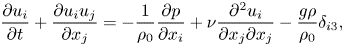 $$\begin{gather}\frac{\partial u_{i}}{\partial t} +\frac{\partial u_{i}u_{j}}{\partial x_{j}} ={-} \frac{1}{\rho_0} \frac{\partial p}{\partial x_{i}} +\nu\frac{\partial^{2} u_{i}}{\partial x_{j}\partial x_{j}} -\frac{g\rho}{\rho_0}\delta_{i3}, \end{gather}$$
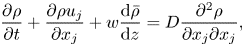 $$\begin{gather}\frac{\partial \rho}{\partial t} +\frac{\partial \rho u_{j}}{\partial x_{j}} +w\frac{{\rm d}\bar{\rho}}{{\rm d} z} = D\frac{\partial^{2} \rho}{\partial x_{j}\partial x_{j}}, \end{gather}$$
where  $u_{i}$ is the $i$th component of the velocity vector, $p$ is the pressure, $\rho _0$ is the constant mean density, $D$ is the diffusivity coefficient for density, $\delta _{ij}$ is the Kronecker's delta and $g$ is the gravitational acceleration. The subscripts $i=1,2$ and 3 denote $x$,
$x$,  $y$ and $z$ directions, respectively, and the velocity components in these directions are denoted by $u$,
$u$,  $v$ and $w$.
$w$.
The decay of freely evolving, stably stratified homogeneous turbulence is considered in this study. Here, we introduce several important parameters of the flow. An average of a variable  $f$ is defined as a volume average $\langle\, f\rangle _V(t) =V^{-1}\iiint f(x,y,z,t)\,{\rm d} x\,{\rm d} y\,{\rm d} z$, where $V$ is the integral volume. A velocity scale of large-scale horizontal motions is defined as $U_{H}=\langle u^2\rangle _V^{1/2}$. The integral scales in the horizontal and vertical directions are denoted by $L_H$ and $L_V$, respectively, and are defined with the autocorrelation functions of horizontal velocity as
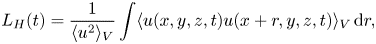 $$\begin{gather} L_H(t)=\frac{1}{\langle u^2\rangle_V}\int\langle u(x ,y,z,t) u(x+r,y,z,t)\rangle_V \,{\rm d} r, \end{gather}$$
 $$\begin{gather}L_V(t)=\frac{1}{\langle u^2\rangle_V}\int\langle u(x,y,z ,t) u(x,y,z+r,t)\rangle_V \,{\rm d} r. \end{gather}$$
 For the linear density profile of  $\bar {\rho }$, the mean potential energy is defined as $E_P=\langle b^2\rangle _V/2$ with the buoyancy $b=\rho g/\rho _0 N$. The governing equations for kinetic energy $k_T=\langle u_iu_i\rangle _V/2$ and potential energy are given by
 $$\begin{gather} \frac{\partial k_T}{\partial t} ={-}\langle 2\nu {\mathsf{S}}_{ij}{\mathsf{S}}_{ij}\rangle_V -\frac{g}{\rho_0}\langle w\rho\rangle_V, \end{gather}$$
 $$\begin{gather}\frac{\partial E_P}{\partial t} ={-}D\langle \boldsymbol{\nabla} b\boldsymbol{\cdot}\boldsymbol{\nabla} b\rangle_V +\frac{g}{\rho_0}\langle w\rho\rangle_V. \end{gather}$$
The second terms on the right-hand side of these equations are the buoyancy flux and represent the energy exchange between kinetic energy and potential energy. The dissipation rates of  $k_T$ and $E_P$ are given by $\varepsilon =\langle 2\nu {\mathsf{S}}_{ij}{\mathsf{S}}_{ij}\rangle _V$ and $\varepsilon _P=D\langle \boldsymbol {\nabla } b\boldsymbol {\cdot}\boldsymbol {\nabla } b\rangle _V$, where ${\mathsf{S}}_{ij}=(\partial u_i/\partial x_j+\partial u_j/\partial x_i)/2$ is a rate-of-strain tensor.
The Kolmogorov scale represents the smallest scale of turbulent motions and is defined by  $\eta =(\nu ^3/\varepsilon )^{1/4}$. It is often considered that the stratification significantly suppresses vertical turbulent motions at scales greater than the Ozmidov scale, which is defined as $L_O=(\varepsilon /N^3)^{1/2}$ with $N=\sqrt {-(g/\rho _0)\,{\rm d}\bar {\rho }/{\rm d} z}$. The relative strength of stratification is evaluated with the horizontal Froude number $Fr_H=U_H/L_HN$, which is defined as the ratio between the buoyancy period $1/N$ and the time scale of large-scale horizontal motions $L_H/U_H$. The buoyancy Reynolds number is defined with the length scale ratio between $L_O$ and $\eta$ as
 \begin{equation} Re_b=\left(\frac{L_O}{\eta}\right)^{4/3}=\frac{\varepsilon}{N^2\nu}. \end{equation}
Turbulent motions at scales below  $L_O$ are not significantly suppressed by the stable stratification, and there is a range of scales with small-scale turbulent fluctuations if $Re_b\gg {{O}}(10^0)$. On the other hand, the small-scale turbulent motions are also inhibited by the stratification for $Re_b\leq {{O}}(10^0)$. The Reynolds number of large-scale horizontal motions can be defined as $Re_H=U_{H}L_{H}/\nu$. It should be noted that one can relate $Re_b$ to $Re_H$ and $Fr_H$ as $Re_b\sim Re_H Fr_H^2$ with the dissipation scaling $\varepsilon \sim U_{H}^3/L_H$, which is often assumed for stratified turbulence (Riley & de Bruyn Kops Reference Riley and de Bruyn Kops2003; Brethouwer et al. Reference Brethouwer, Billant, Lindborg and Chomaz2007).
2.1. Decay laws of Saffman and Batchelor turbulence at high  $Re_b$

First, we briefly review the decay laws derived in Davidson (Reference Davidson2009, Reference Davidson2010) for Saffman and Batchelor turbulence in a stably stratified fluid at high  $Re_b$. Davidson (Reference Davidson2010) adapted the theory of axisymmetric Saffman turbulence to freely evolving, stably stratified homogeneous turbulence and obtained
 \begin{equation} U_{H}^2 L_H^2 L_V=\mathrm{Const.}, \end{equation}
which is required for the Saffman-like invariant to be constant when the large scales evolve in a self-similar manner. Similarly, the following constraint was derived for axisymmetric Batchelor turbulence in a stably stratified fluid (Davidson Reference Davidson2009):
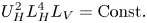 \begin{equation} U_{H}^2 L_H^4 L_V=\mathrm{Const.} \end{equation}
This is also required for the Loitsyansky-like integral to be constant.
Equations (2.9) and (2.10) are satisfied during the decay and are directly related to the decay law of stably stratified homogeneous turbulence. The cases with high  $Re_b\sim Re_H Fr_H^2$ with low $Fr_H$ and high $Re_H$ were considered in Davidson (Reference Davidson2009, Reference Davidson2010), where the following assumptions were made:
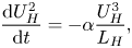 $$\begin{gather} \frac{{\rm d} U_{H}^2}{{\rm d} t}={-}\alpha\frac{U_{H}^3}{ L_H}, \end{gather}$$
 $$\begin{gather}\frac{U_{H}}{N L_V }=C. \end{gather}$$
Here  $\alpha$ and $C$ are dimensionless constants of order one. The first assumption concerns the non-dimensional kinetic energy dissipation rate $\alpha =\varepsilon L_H/U_{H}^3$, while the second one can be derived from the balance between inertial and buoyancy forces for ${Re_b\sim Re_H Fr_H^2\gg 1}$ (Lindborg Reference Lindborg2006). Equations (2.11) and (2.12) combined with (2.9) yield the following power laws for axisymmetric Saffman turbulence in a stably stratified fluid (Davidson Reference Davidson2010):
 \begin{equation} U_{H}^2 \sim t^{{-}4/5},\quad L_H \sim t^{ 3/5},\quad L_V \sim t^{{-}2/5},\quad \varepsilon \sim t^{{-}9/5}. \end{equation}
On the other hand, (2.10), (2.11) and (2.12) yield the following decay laws for Batchelor turbulence (Davidson Reference Davidson2009):
 \begin{equation} U_{H}^2 \sim t^{{-}8/7},\quad L_H \sim t^{3/7},\quad L_V \sim t^{{-}4/7},\quad \varepsilon \sim t^{{-}15/7}. \end{equation}
The decay of  $U_H^2$ is slower than non-stratified isotropic turbulence, for which $U^2 \sim t^{-6/5}$ in Saffman turbulence and $U^2 \sim t^{-10/7}$ in Batchelor turbulence. Furthermore, the integral scale increases as non-stratified isotropic turbulence decays while $L_V$ decreases with time in (2.13a–d) and (2.14a–d).
In addition to the above power laws obtained by Davidson (Reference Davidson2009, Reference Davidson2010), we can also derive the decay laws of potential energy for Saffman and Batchelor turbulence. From the balance between the pressure gradient and the buoyancy term in the governing equation of  $w$, one can assume that the density perturbation $\rho$ is scaled by $U_H^2 \rho _{0}/g L_V$ (Godoy-Diana, Chomaz & Billant Reference Godoy-Diana, Chomaz and Billant2004), or equivalently,
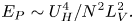 \begin{equation} E_P \sim U_H^4/N^2L_V^2. \end{equation}
This scaling combined with (2.13a–d) or (2.14a–d) yields the following power laws for the decay of  $E_P$ at high $Re_b$:
 $$\begin{gather} E_P\sim t^{{-}4/5}\quad \text{for high-}Re_b\ \text{Saffman turbulence}, \end{gather}$$
 $$\begin{gather}E_P\sim t^{{-}8/7}\quad \text{for high-}Re_b\ \text{Batchelor turbulence}. \end{gather}$$
The decay exponents of  $E_P$ are the same as those of $U_{H}^2$. The kinetic energy $k_T$ is dominated by the horizontal velocity in strongly stratified turbulence, and, therefore, the ratio $E_P/k_T$ is constant during the decay.
2.2. Alternative decay laws for low $Re_b$

The above decay laws derived for high  $Re_b$ have not been verified in stably stratified grid turbulence most probably because the Reynolds number is not sufficiently high in experiments. For example, Praud et al. (Reference Praud, Fincham and Sommeria2005) found that $L_V$ increases with time in the towed-grid experiments while $L_V$ is expected to decrease for high- $Re_b$ Saffman and Batchelor turbulence. In this section we derive the decay laws of stably stratified homogeneous turbulence at low $Re_b$, which should be more relevant to most experimental studies of decaying stratified turbulence. Stratified turbulence at low $Re_b$ is often referred to as the viscosity-affected stratified flow regime (Brethouwer et al. Reference Brethouwer, Billant, Lindborg and Chomaz2007). For this regime, Godoy-Diana et al. (Reference Godoy-Diana, Chomaz and Billant2004) assumed that the vertical length scale is determined as a result of the balance between the horizontal advection and the vertical diffusion and proposed the relation between $L_H$ and $L_V$ given by $L_V \sim L_H Re_H^{-1/2}$. From the definition of $Re_H$ one can expect the following relation during the decay:
 \begin{equation} L_V \sim \left(\nu\frac{L_H}{U_H}\right)^{1/2}. \end{equation}
Here  $\nu$ is treated as a constant parameter in each flow. When the kinetic energy dissipation is assumed to be dominated by the vertical gradient of horizontal velocity at low $Re_b$, the dissipation rate is estimated as $\varepsilon \sim \nu U_H^2/L_V^2$. This relationship can be combined with (2.18) to derive $\varepsilon \sim U_H^3/L_H$, which leads to (2.11) even for low $Re_b$ (Brethouwer et al. Reference Brethouwer, Billant, Lindborg and Chomaz2007; Maffioli & Davidson Reference Maffioli and Davidson2016). Then, (2.11) and (2.18) combined with (2.9) yield the following decay laws of Saffman turbulence at low $Re_b$:
 \begin{equation} U_{H}^2 \sim t^{{-}5/4},\quad L_H \sim t^{3/8},\quad L_V \sim t^{1/2},\quad \varepsilon \sim t^{{-}9/4}. \end{equation}
For the Batchelor turbulence, the following decay laws are derived with (2.10), (2.11) and (2.18):
 \begin{equation} U_{H}^2 \sim t^{{-}3/2},\quad L_H \sim t^{ 1/4},\quad L_V \sim t^{ 1/2},\quad \varepsilon \sim t^{{-}5/2}. \end{equation}
Here, the decay laws of  $\varepsilon$ are derived from $\varepsilon = \alpha U_{H}^3/L_H$ with a constant $\alpha$.
As also discussed for high- $Re_b$ cases, the decay laws of $E_P$ can be derived from $E_P \sim U_H^4/N^2L_V^2$ combined with (2.19a–d) or (2.20a–d). These decay laws can be written as
 $$\begin{gather} E_P\sim t^{{-}7/2}\quad \text{for low-}Re_b\ \text{Saffman turbulence}, \end{gather}$$
 $$\begin{gather}E_P\sim t^{{-}4}\quad \text{for low-}Re_b\ \text{Batchelor turbulence}. \end{gather}$$
In this study it will be shown that these decay laws for low- $Re_b$ Saffman turbulence prevail in stably stratified grid turbulence at low Froude numbers.
3. Direct numerical simulations of temporally evolving stably stratified grid turbulence
3.1. Temporally evolving stably stratified grid turbulence
Direct numerical simulations are carried out for a numerical model of towed-grid experiments conducted by Praud et al. (Reference Praud, Fincham and Sommeria2005) and Fincham et al. (Reference Fincham, Maxworthy and Spedding1996). Here, we consider a temporally evolving grid turbulence as an approximation of the grid turbulence generated by a towed grid. Non-stratified, temporally evolving grid turbulence was studied with DNS in Watanabe & Nagata (Reference Watanabe and Nagata2018), where the evolutions of various velocity statistics were shown to be quantitatively consistent with wind-tunnel experiments and towed-grid experiments without density stratification. The grid considered in the present DNS is a rake of vertical flat plates with a mesh size  $M$ (Praud et al. Reference Praud, Fincham and Sommeria2005). The thickness of each plate $D$ is $0.2M$, which yields a solidity of 0.2. The grid is towed in the horizontal ( $x$) direction at a constant speed $U_0$ in a stably stratified fluid with a constant ${\rm d}\bar {\rho }/{\rm d} z$. Each plate generates a turbulent wake, and the wake interaction results in the formation of grid turbulence.
Simulations of temporally evolving grid turbulence adapt the methodology used to simulate temporally evolving turbulent shear flows, which are also studied as an approximation of spatially evolving counterparts. Temporal simulations of turbulent shear flows use a periodic boundary condition in the streamwise direction, and the flow develops with time instead of the streamwise direction (da Silva & Pereira Reference da Silva and Pereira2008; Pham, Sarkar & Brucker Reference Pham, Sarkar and Brucker2009; Diamessis, Spedding & Domaradzki Reference Diamessis, Spedding and Domaradzki2011; Gampert et al. Reference Gampert, Boschung, Hennig, Gauding and Peters2014; Watanabe et al. Reference Watanabe, Sakai, Nagata, Ito and Hayase2015; Kozul, Chung & Monty Reference Kozul, Chung and Monty2016; Watanabe, Zhang & Nagata Reference Watanabe, Zhang and Nagata2018b). The temporally evolving grid turbulence is also simulated in a triply periodic box (Watanabe & Nagata Reference Watanabe and Nagata2018). Simulations of temporally evolving wakes are often initialized with a top-hat mean velocity profile for which different mean velocity values are applied to the free stream and the wake region behind an object (Zecchetto & da Silva Reference Zecchetto and da Silva2021). Then, the shear due to the mean velocity difference results in the development of the turbulent wake. Following the approach used for temporal wakes, the DNS of temporally evolving grid turbulence is initialized with the following velocity and density profiles (Watanabe & Nagata Reference Watanabe and Nagata2018):
 $$\begin{gather} u(x,y,z,t=0) = \langle u \rangle(\kern0.7pt y,t=0) + u'(x,y,z), \end{gather}$$
 $$\begin{gather}v(x,y,z,t=0) = v'(x,y,z), \end{gather}$$
 $$\begin{gather}w(x,y,z,t=0) = w'(x,y,z), \end{gather}$$
 $$\begin{gather}\rho'(x,y,z,t=0)=0, \end{gather}$$
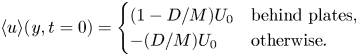 $$\begin{gather}\langle u \rangle(\kern0.7pt y,t=0)= \begin{cases} (1-D/M)U_0 & \text{behind plates}, \\ -(D/M)U_0 & \text{otherwise}. \end{cases} \end{gather}$$
Here,  $\langle\, f \rangle (\kern0.7pt y,t)=(1/L_xL_z)\iint f(x,y,z,t)\,{\rm d} x\,{\rm d} z$ is the average taken on a $x$–
$x$– $z$ plane, where ( $L_x, L_y, L_z$) is the computational domain size, while fluctuations are denoted by $f'=f-\langle\, f \rangle$. Figure 1 shows the initial profile of the mean velocity $\langle u\rangle$. The velocity difference between the two regions is $U_0$ for (3.5). Here, the mean velocity profile is derived by subtracting $(D/M)U_0$ from $U_0$ and 0 so that the volume average of $u$ is zero. This enables us to adapt a large time increment at a late time because the instantaneous velocity becomes small with time. Initial velocity perturbations $(u',v',w')$ are obtained by the method that generates spatially correlated fluctuations from random numbers (Watanabe, Zhang & Nagata Reference Watanabe, Zhang and Nagata2019b; Hayashi, Watanabe & Nagata Reference Hayashi, Watanabe and Nagata2021; Watanabe & Nagata Reference Watanabe and Nagata2021). The characteristic length scale of $(u',v',w')$ is $0.1M$ and the initial r.m.s. velocity fluctuations are $0.005U_0$, which is as small as the background fluctuations in wind-tunnel experiments of grid turbulence (Seoud & Vassilicos Reference Seoud and Vassilicos2007; Kitamura et al. Reference Kitamura, Nagata, Sakai, Sasoh, Terashima, Saito and Harasaki2014). The Brunt–Väisälä frequency $N$ is constant and is not varied with time. Therefore, the initial flow field is already stably stratified. This is contrary to some other simulations of decaying turbulence, which imposes stratification after the turbulence freely decays for a short time without the stratification (Diamessis et al. Reference Diamessis, Spedding and Domaradzki2011; de Bruyn Kops & Riley Reference de Bruyn Kops and Riley2019). Experiments of towed-grid turbulence are prepared by filling a tank with a stratified fluid. Then, the grid is towed in the tank to generate grid turbulence. Wind-tunnel experiments also introduce stable stratification before the flow passes a grid. These situations are better approximated in DNS of temporally evolving grid turbulence by initializing the flow field with a stratified fluid because the generation process of grid turbulence is strongly influenced by stable stratification, as also discussed by Okino & Hanazaki (Reference Okino and Hanazaki2019).
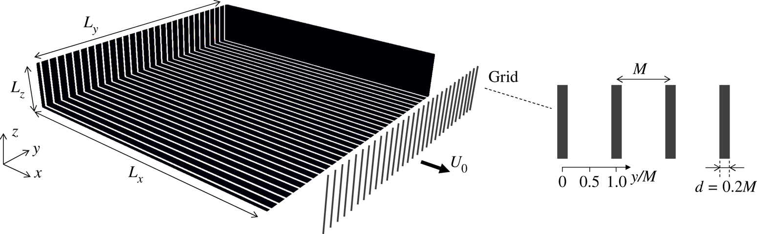
Figure 1. The initial condition of DNS of temporally evolving grid turbulence. White and black regions, shown on the domain boundaries, have the initial mean velocity of  $(1-D/M)U_0$ and $-(D/M)U_0$, respectively. The grid geometry is also shown beside the computational domain. Statistics are calculated between $y/M=0$ and 1.
Most statistics presented in this paper are calculated as functions of  $y$ in the range of $0\leq y/M \leq 1$, as shown in figure 1. Here, the grid consists of a large number of vertical plates. The samples in $0\leq y/M \leq 1$ are taken from all the plates because the wake of each plate is statistically identical. In grid turbulence, $\langle\, f \rangle (\kern0.7pt y,t)$ is different from the volume average $\langle\, f\rangle _V(t)$ in the near-grid region, which corresponds to an early time of temporally evolving grid turbulence. Once grid turbulence has fully developed, the statistics do not depend on $y$. Then, $\langle\, f \rangle (\kern0.7pt y,t)$ is identical to $\langle\, f\rangle _V(t)$. The decay laws of grid turbulence are examined with the statistics defined with the $x$–
$x$– $z$ average $\langle\, f \rangle (\kern0.7pt y,t)$ while the volume average is used for comparison with experimental data.
3.2. Numerical methods and parameters
The temporally evolving grid turbulence is simulated with the DNS code that solves (2.1)–(2.3) with the fractional step method. This code has been used in our previous studies on homogeneous isotropic turbulence and stably stratified turbulent shear layers (Watanabe et al. Reference Watanabe, Riley, Nagata, Onishi and Matsuda2018a, Reference Watanabe, Riley, Nagata, Matsuda and Onishi2019a; Watanabe, Tanaka & Nagata Reference Watanabe, Tanaka and Nagata2020). Spatial derivatives are computed with the fully conservative fourth-order central difference scheme (Morinishi et al. Reference Morinishi, Lund, Vasilyev and Moin1998). Time is advanced with a third-order Runge–Kutta method. The biconjugate gradient stabilized method is used to solve the Poisson equation for pressure.
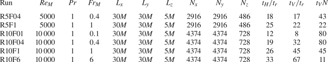
Table 1 summarizes the computational parameters of DNS. The stably stratified grid turbulence can be characterized by the Reynolds number  $Re_M$, Prandtl number $Pr$ and Froude number $Fr_M$ defined as
Table 1. Computational and physical parameters of DNS. The size of the computational domain is  $(L_x,L_y,L_z)$, which is represented by $N_x\times N_y\times N_z$ grid points. At time $t_H$, the production rate of turbulent kinetic energy becomes smaller than 1 % of the dissipation rate as examined in figure 8. The time at which the flow enters a viscosity-affected stratified flow regime is denoted by $t_V$, which is obtained from figure 9. Time $t_V$ is normalized by the reference time scale of grid turbulence $t_r$ or the buoyancy period $1/N$.
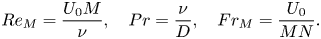 \begin{equation} Re_M= \frac{U_0 M}{\nu},\quad Pr = \frac{\nu}{D},\quad Fr_M= \frac{U_0}{MN}. \end{equation}
Direct numerical simulation is performed for five sets of  $(Re_M,Fr_M)$ with $Pr=1$. The simulations are performed until $t/t_r=250$, where $t_r=M/U_0$ is the characteristic time scale. This normalization $t/t_r$ is useful because the normalized streamwise distance from a grid in wind-tunnel experiments, $x/M$, is equivalent to $t/t_r$, where $x/U_0=t$ is the advection time from the grid to the location $x$. The domain size with $L_x,L_y>L_z$ is used because the horizontal integral scales are much larger than the vertical scale in stably stratified turbulence. The integral scales increase with time. However, even at the end of simulations, the domain size is larger than 12 times the integral length scales, which is large enough to prevent the confinement effects on the decay of turbulence (Anas, Joshi & Verma Reference Anas, Joshi and Verma2020). The number of the grid points $(N_x,N_y,N_z)$ is determined based on the Kolmogorov scale $\eta$. The kinetic energy dissipation rate in grid turbulence is evaluated as $\varepsilon = \nu \langle (\partial u'_{i}/\partial x_j)^2\rangle$ because the flow is initially inhomogeneous. The grid spacing $\varDelta$ is uniform in three directions. The Kolmogorov scale becomes the smallest in the production phase of grid turbulence and increases with time as the turbulence decays. The largest value of $\varDelta /\eta$ is about 1.6 at $t/t_r\approx 7$, at which the flow is highly inhomogeneous, and $\varDelta /\eta$ becomes smaller than 1 when grid turbulence has fully developed. Small-scale fluctuations of turbulence are well resolved with this resolution for the present schemes (Watanabe et al. Reference Watanabe, Riley, Nagata, Onishi and Matsuda2018a). The time increment $\Delta t$ is determined with a constant Courant number $\mathrm {CFL}=0.3$, which is also small enough to capture wave motions with the frequency $N$.
$N$.
4. Results and discussion
4.1. Development of stably stratified grid turbulence
Figure 2 visualizes the development of grid turbulence in R10F1. The left panels show the colour contour of  $u$ on the surfaces of the computational domain while the right panels visualize $u$ on a small part of an $x$–
$x$– $y$ plane. At $t/t_r=5$ in ( $a$), the instantaneous velocity profiles are strongly influenced by the wakes of the vertical plates. The wakes develop with time and interact with each other, resulting in the formation of the fully developed grid turbulence. Figure 3 visualizes $u$ on a vertical plane at $t/t_r=15$ in R10F01 and R10F6. The strongly stable stratification at $Fr_M=0.1$ causes highly anisotropic velocity fluctuations. However, more isotropic distribution of $u$ is found for $Fr_M=6$. For both $Fr_M$, the imprints of the wakes are hardly seen in the velocity profiles, and the grid turbulence has developed by this time.
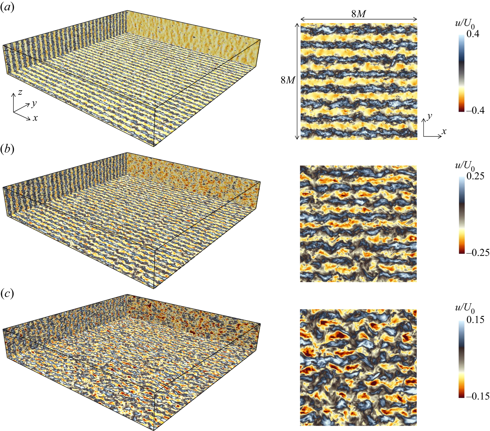
Figure 2. Development of temporally evolving grid turbulence in R10F1 at (a)  $t/t_r=5$, (b) $t/t_r=10$ and (c) $t/t_r=15$. The streamwise velocity $u$ is visualized on the boundaries of the computational domain on the left panels while two-dimensional contours of $u$ on an $x$–
$x$– $y$ plane are shown on the right panels.
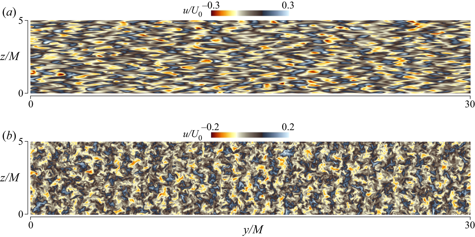
Figure 3. Streamwise velocity profiles on a vertical plane in (a) R10F01 and (b) R10F6 at  $t/t_r=15$.
Figure 4 compares the temporal evolution of volume-averaged horizontal kinetic energy  $\langle u^2+v^2\rangle _V/2$ between the DNS and experiments of towed-grid experiments by Praud et al. (Reference Praud, Fincham and Sommeria2005), where the average is taken in the computational domain of DNS or the measurement volume of scanning particle image velocimetry. The experiments were conducted in a water tank, where the density stratification was generated with saltwater. Therefore, the Schmidt number was much larger than 1 in the experiments while all DNS consider $Pr=1$, and this difference may affect the comparison between the DNS and experiments. Figure 4 shows that the horizontal kinetic energy decreases with time. The present DNS with small $Fr_M$ agrees well with the experiments, which were also conducted with $Fr_M\approx 0.1$. The horizontal kinetic energy contains the contribution from both mean and fluctuating velocity components. When the grid turbulence is generated, the kinetic energy in the mean velocity is converted to that of the velocity fluctuations by the production term of turbulent kinetic energy, which is expressed as the product of the Reynolds stress and the mean velocity gradient. The decay of horizontal velocity fluctuations is caused by the viscous dissipation once grid turbulence has fully developed. Although the mean velocity profile given as the initial condition of DNS is only a simple approximation of the flow behind a grid, the initial decay of $\langle u^2+v^2\rangle _V/2$ is in good agreement between the DNS and the experiments. In the DNS the horizontal kinetic energy tends to be small for large $Fr_M$, while the $Re_M$ dependence is not significant for a fixed value of $Fr_M$. The energy production by the mean velocity gradient contributes to the growth of the streamwise velocity component of turbulent kinetic energy, which is converted to the other components by the pressure-strain correlation (Pope Reference Pope2000). This conversion to the vertical component is suppressed in a stably stratified fluid, and a smaller amount of horizontal kinetic energy is converted to the vertical component at lower $Fr_M$ during the production phase of grid turbulence. This stratification effect explains larger $\langle u^2+v^2\rangle _V/2$ for smaller $Fr_M$.
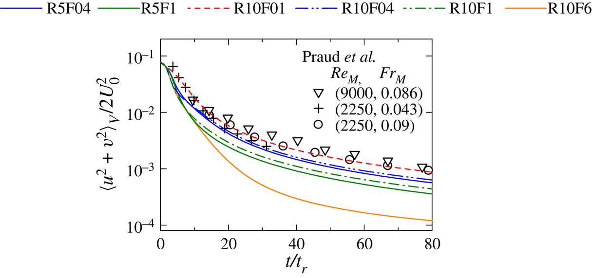
Figure 4. Temporal evolutions of volume-averaged horizontal kinetic energy  $\langle u^2+v^2\rangle _V/2$ compared with towed-grid experiments by Praud et al. (Reference Praud, Fincham and Sommeria2005).
Figure 5 shows the lateral profiles of mean velocity  $\langle u\rangle$ and r.m.s. velocity fluctuations $u_{rms}=\langle u'^2\rangle ^{1/2}$. The turbulent wake develops for $0\leq y/M \leq 0.1$ and $0.9\leq y/M \leq 1$ and the mean velocity difference between the wake and the open region of the grid becomes small with time. The mean velocity profile is homogeneous at $t/t_r=25$. The velocity fluctuations in the $x$ direction are generated by the mean velocity gradient, which is large at $y/M=0.1$ and 0.9 at $t/t_r=2$. Therefore, $u_{rms}$ also reaches peaks at these locations. The wakes spread in the $y$ direction and merge with the adjacent wakes. The profile of $u_{rms}$ also becomes homogeneous at $t/t_r=25$, and $u_{rms}$ decays with time.
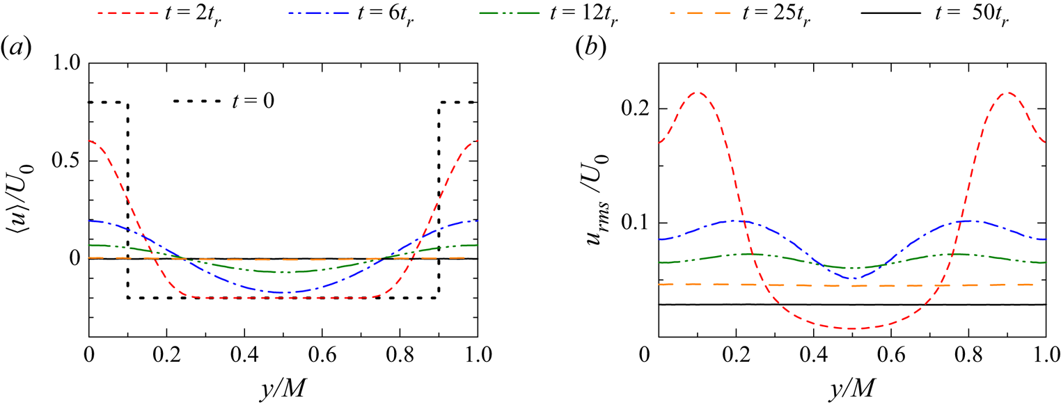
Figure 5. Lateral profiles of (a) mean velocity  $\langle u\rangle$ and (b) r.m.s. velocity fluctuations $u_{rms}$ in R10F1. The results are taken at five instances of $t/t_r=2$, 6, 12, 25 and 50.
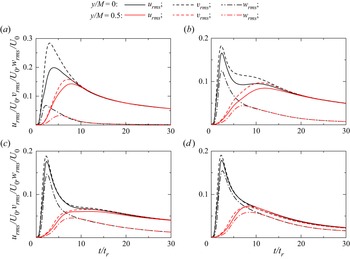
Figure 6 compares the temporal evolutions of the r.m.s. fluctuations of three velocity components ( $u_{rms}$, $v_{rms}$ and $w_{rms}$) at $y/M=0$ and 0.5. Here, the results are also compared among different $Fr_M$ for $Re_M=10\,000$. As the turbulence is generated at an early time, the r.m.s. velocity fluctuations increase with time. This increase is more rapid at $y/M=0$ than at $y/M=0.5$ because the turbulent wake of each plate develops at $y/M=0$. Then, they begin to decrease as the turbulence decays. At a late time, the r.m.s. velocity fluctuations hardly differ at $y/M=0$ and $0.5$ and the flow reaches a statistically homogeneous state. Furthermore, the horizontal velocity fluctuations become isotropic ( $u_{rms}\approx v_{rms}$). The time required for stably stratified grid turbulence to be homogeneous and isotropic in the horizontal directions is different depending on $Fr_M$. This time is about $10t_r$, $20t_r$, $25t_r$ and $10t_r$ for $Fr_M=0.1$, 0.4, 1 and 6, respectively. For $Fr=0.1$ and 6, the r.m.s. velocity fluctuations monotonically decrease after they reach the peaks. However, $u_{rms}$ and $v_{rms}$ for $Fr_M=0.4$ and 1 hardly decrease with time for $7\lesssim t/t_r \lesssim 12$ after the rapid decay from the peak at $t/t_r\approx 4$. This tendency is clearer for $y/M=0$ in the wakes of vertical plates. Therefore, the slow decay for $7\lesssim t/t_r \lesssim 12$ might be related to the decay characteristics of the wake.
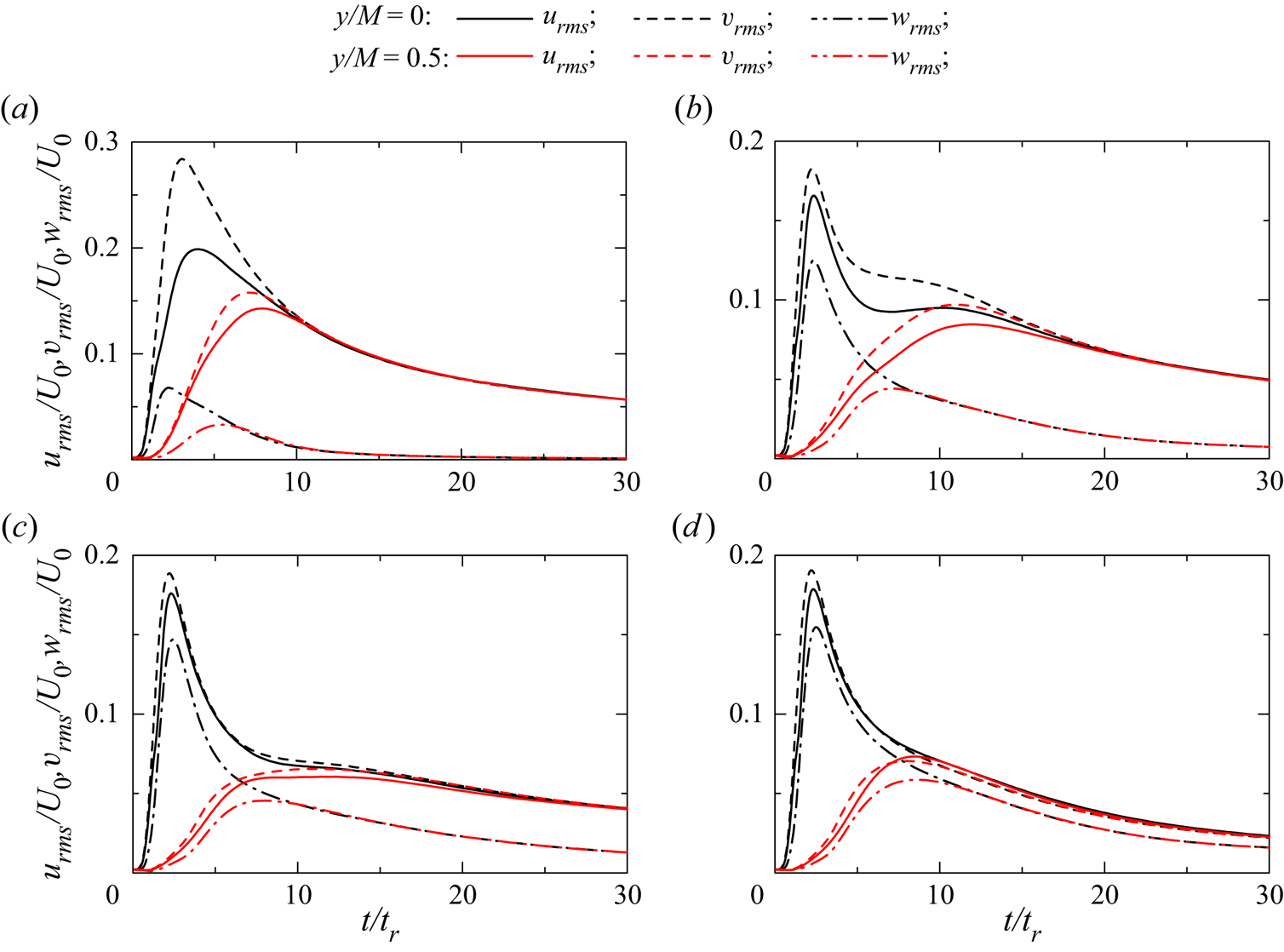
Figure 6. Temporal evolutions of r.m.s. velocity fluctuations at  $y/M=0$ and 0.5 in the cases of (a) R10F01, (b) R10F04, (c) R10F1 and (d) R10F6.
Figure 7(a) presents  $u_{rms}/U_0$ as a function of time normalized by the buoyancy period $N^{-1}$. A comparison between figures 6 and 7(a) suggests that the initial growth of the r.m.s. velocity fluctuations is better characterized by $t_r$. The time interval corresponding to the slow decay of $u_{rms}$ is found for $14\lesssim tN \lesssim 30$ for $Fr=0.4$ and $7\lesssim tN \lesssim 20$ for $Fr=1$. Experiments and numerical simulations of a turbulent wake of a sphere in a stably stratified fluid have reported that the wake development can be divided into three regimes: a three-dimensional regime for $0\leq tN \leq 2$, a non-equilibrium (NEQ) regime for $2\leq tN \leq 50$ and a quasi-two-dimensional regime for $50\leq tN$ (Spedding Reference Spedding1997; Diamessis et al. Reference Diamessis, Spedding and Domaradzki2011). The decay rates of the mean velocity deficit and r.m.s. velocity fluctuations are different among these regimes. Zhou & Diamessis (Reference Zhou and Diamessis2019) showed that the decay of the horizontal r.m.s. velocity fluctuations becomes slow for $10\lesssim tN\lesssim 50$, which is within the NEQ regime. In the present DNS, the range of $10\leq tN\leq 50$ corresponds to $4\leq t/t_r \leq 20$ for $Fr_M=0.4$ and $10\leq t/t_r \leq 50$ for $Fr_M=1$. The slow decays of $u_{rms}$ and $v_{rms}$ are observed within these intervals. In contrast, the NEQ regime corresponds to $1\leq t/t_r \leq 5$ for $Fr_M=0.1$ and $60\leq t/t_r \leq 300$ for $Fr_M=6$. When the turbulent wake is being generated, $u_{rms}$ at $y=0$ increases with time. Once the turbulent wake has developed, $u_{rms}$ begins to decay and the interaction of the turbulent wakes generates homogeneous turbulence, where $u_{rms}$ does not depend on $y$. In figure 7(a), $u_{rms}$ in R10F01 increases with time for the time corresponding to the possible NEQ regime ( $10\lesssim tN\lesssim 50$). Therefore, the NEQ regime is over before the turbulent wake has developed. On the other hand, $u_{rms}$ in R10F6 hardly differs for $y/M=0$ and 0.5 in the NEQ regime and decreases with time, suggesting that homogeneous turbulence has developed for $Fr_M=6$ before the wake reaches the NEQ regime. Thus, the slow decay during the NEQ regime of stratified wakes is not observed for $Fr_M=0.1$ and 6. It should be noted that the discussions are based on the studies on the stratified wake of a sphere, which is different from the wake of a vertical plate considered in this study. The slow decay in the NEQ regime is only one of the possible explanations for the behaviour $u_{rms}$ and $v_{rms}$.
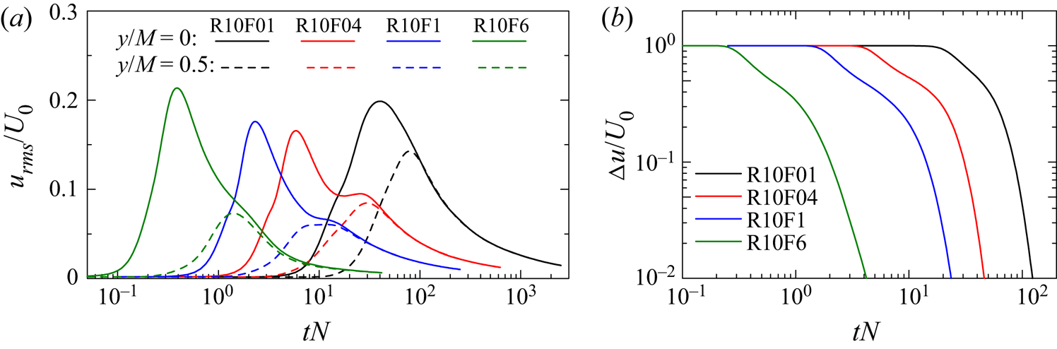
Figure 7. Temporal evolutions of (a)  $u_{rms}/U_0$ at $y/M=0$ and 0.5, and (b) the mean velocity deficit of the wake, $\Delta u$, which are plotted as functions of $tN$.
$tN$.
The wake development of each plate can also be evaluated with the mean velocity deficit  $\Delta u$, which is defined as the difference in $\langle u\rangle$ between $y/M=0$ and 1. Figure 7(b) shows $\Delta u$ as a function of $tN$. In a freely developing wake of an object, such as a sphere and a cylinder, $\Delta u$ becomes small with time although $\Delta u$ does not reach zero. The wakes are generated by many plates in the case of grid turbulence. Therefore, $\Delta u$ in grid turbulence rapidly decreases to zero with time. In a stably stratified wake of a sphere, the decay of $\Delta u$ becomes slower once the flow enters the NEQ regime (Spedding Reference Spedding1997). The decay of $\Delta u$ for R10F04 and R10F1 becomes slightly slower at $tN\approx 10$ and 5, respectively, than at an earlier time. However, the change of the decay rate is less clear than that reported for stably stratified wakes. This might be partially due to the interaction with adjacent wakes, which results in $\Delta u\rightarrow 0$ while $\Delta u$ in a conventional wake is greater than 0 even at a late time.
The budget of the turbulent kinetic energy  $k_T(\kern0.7pt y,t)= ( \langle u'^2\rangle +\langle v'^2\rangle +\langle w'^2\rangle )/2$ is examined with the transport equation of $k_T$. Once the grid turbulence has developed, the production rate of $k_T$ becomes much smaller than the dissipation rate. Here, an average in the $y$ direction is defined for a statistical quantity $F(\kern0.7pt y,t)$ as $\bar {F}(t)=(1/L_y)\int F(\kern0.7pt y,t)\,{{\rm d}y}$. The spatially averaged turbulent kinetic energy $\overline {k_T}$ evolves following the equation given by
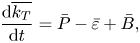 \begin{equation} \frac{{\rm d} \overline{k_T}}{{\rm d} t} =\bar{P}-\bar{\varepsilon} + \bar{B}, \end{equation}
where  $P$,
$P$,  $\varepsilon$ and $B$ are the production, dissipation and buoyancy flux in the transport equation of $k_T(\kern0.7pt y,t)$,
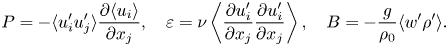 \begin{equation} P={-} \langle u'_{i}u'_{j} \rangle \frac{\partial \langle u_i\rangle}{\partial x_j},\quad \varepsilon= \nu\left\langle\frac{\partial u'_{i}}{\partial x_j} \frac{\partial u'_{i}}{\partial x_j}\right\rangle,\quad B={-} \frac{g}{\rho_0}\langle w'\rho'\rangle. \end{equation}
Here,  $\varepsilon$ and $B$ are identical to the first and second terms of (2.6), respectively, when the flow is statistically homogeneous. Figure 8(a) shows the temporal evolutions of $\bar {P}$, $\bar {\varepsilon }$ and $\bar {B}$ for R10F1. Initially, $\bar {P}$ is larger than $\bar {\varepsilon }$ until $t/t_r\approx 3$ because the turbulent kinetic energy is initially small and increases due to the production term. Until grid turbulence has developed by the wake interaction, $\bar {P}$ and $\bar {\varepsilon }$ are comparable for $3\lesssim t/t_r\lesssim 10$. This relationship of $\bar {P}\sim \bar {\varepsilon }$ is widely observed in turbulent free shear flows, where the ratio between the production and dissipation terms of turbulent kinetic energy is close to 1 (Panchapakesan & Lumley Reference Panchapakesan and Lumley1993; Taveira & da Silva Reference Taveira and da Silva2013; Watanabe et al. Reference Watanabe, Sakai, Nagata and Ito2016). Then, $\bar {P}$ rapidly decreases because the mean velocity gradient ${\partial \langle u\rangle }/{\partial y}$ and the Reynolds stress $\langle u'v'\rangle$ become small as grid turbulence develops into a statistically homogeneous state. Because the buoyancy flux $\bar {B}$ is always negative, $-\bar {B}$ is shown in the figure. Positive values of $-\bar {B}$ suggest that the turbulent kinetic energy is converted to the potential energy. However, $-\bar {B}$ is smaller than $\bar {\varepsilon }$ and the decay of the turbulent kinetic energy is dominated by $\bar {\varepsilon }$. In all DNS, $\bar {\varepsilon }$ is at least 10 times larger than $-\bar {B}$ in the decay period of grid turbulence. Figure 8(b) shows the temporal evolutions of $\bar {P}/\bar {\varepsilon }$. The ratio with $\bar {P}/\bar {\varepsilon }\approx 10^{0}$ is observed for $3\lesssim t/t_r\lesssim 10$ except for R10F01, for which $\bar {P}/\bar {\varepsilon }$ begins to decay at an earlier time than for other cases. In all DNS, $\bar {P}/\bar {\varepsilon }$ rapidly decreases because of the development of grid turbulence. However, a comparison between different $Fr_M$ suggests that the rapid decrease of $\bar {P}/\bar {\varepsilon }$ occurs at an earlier time for lower $Fr_M$. Table 1 includes time $t_H$ at which $\bar {P}/\bar {\varepsilon }$ becomes smaller than 0.01. Beyond this time, turbulence is nearly homogeneous and the production of turbulent kinetic energy is almost negligible. The Reynolds number hardly affects $t_H$, which increases with $Fr_M$. Therefore, the grid turbulence reaches a homogeneous state faster under stronger stable stratification. Figures 9(a,b) present the temporal evolutions of $Fr_H=u_{rms}/L_uN$ and $Re_H=u_{rms}L_u/\nu$ at $y/M=0$, where $L_u$ is the longitudinal integral scale defined with $u$. After $Fr_H$ increases by the development of grid turbulence, it monotonically decays. Comparison among all DNS cases suggests that $Fr_H$ depends on $Fr_M$ and does not exhibit a strong dependence on $Re_M$. Similarly, $Re_H$ reaches a peak when turbulence is generated. However, the decay of $Re_H$ is much slower than that of $Fr_H$ because $L_u$ increases with time. Figure 9(c) shows the buoyancy Reynolds number $Re_b$ at $y/M=0$. Except for $Fr_M=0.1$, $Re_b$ exceeds $10$ during the turbulence-production phase. Then, $Re_b$ rapidly decreases to $Re_b<10^0$ for $Fr_M=0.4$ and 1. However, the grid turbulence with $Fr_M=6$ has $Re_b>10^0$ until $t/t_r\approx 70$, and small-scale turbulent motions are active in the early decay period. For $Fr_M=0.1$, $Re_b$ does not exceed $10^0$ even at an early time, and three-dimensional small-scale turbulence is inhibited even when the turbulence is generated.
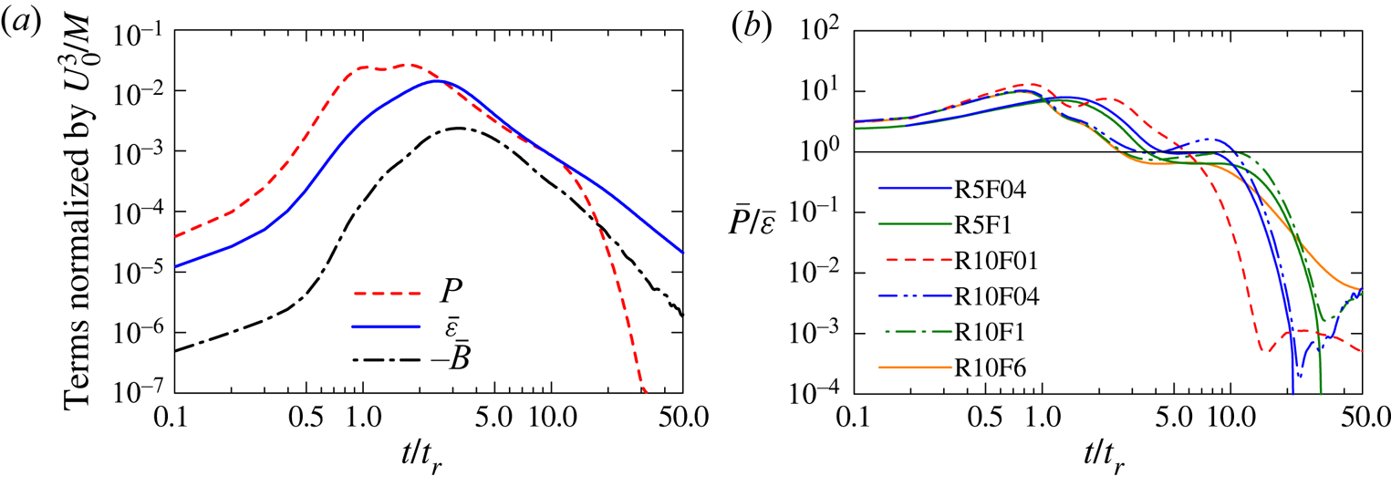
Figure 8. Temporal evolutions of (a) the spatially averaged budget of turbulent kinetic energy for R10F1 and (b) the ratio between the production and dissipation terms  $\bar {P}/\bar {\varepsilon }$.
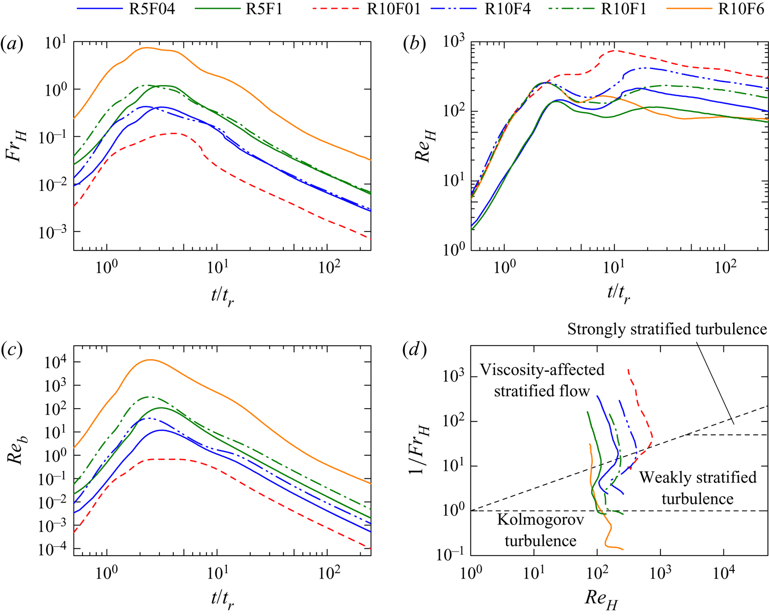
Figure 9. Temporal evolutions of (a) horizontal Froude number  $Fr_H$, (b) Reynolds number based on the horizontal integral scale $Re_H$ and (c) buoyancy Reynolds number $Re_b$ at $y/M=0$. (d) The relation between $Re_H$ and $1/Fr_H$ during the decay of grid turbulence at $y/M=0$.
It is useful to diagnose stably stratified turbulence in the parameter space of  $(Re_H, Fr_H^{-1})$ (Brethouwer et al. Reference Brethouwer, Billant, Lindborg and Chomaz2007). Figure 9(d) shows the trajectory of $(Re_H, Fr_H^{-1})$ during the decay at $y/M=0$ after the peak of $Re_b$. The broken lines distinguish four regimes of stratified turbulence proposed in Brethouwer et al. (Reference Brethouwer, Billant, Lindborg and Chomaz2007): viscosity-affected stratified flow, strongly stratified turbulence, weakly stratified turbulence and classical Kolmogorov turbulence. The two horizontal broken lines represent $Fr_H=1$ and 0.02 while the diagonal broken line is $Re_{H}Fr_{H}^2=1$. As discussed above, $Re_{H}Fr_{H}^2$ is close to $Re_b$ when $\alpha =\varepsilon /(U_{H}^3/L_H)\sim 10^{0}$, and the plots of $(Re_H, Fr_H^{-1})$ complement the temporal evolution of $Re_b$. For $(Re_M, Fr_M)=(10\,000,6)$, the decay of turbulence begins in the classical Kolmogorov turbulence regime, enters the weakly stratified turbulence regime and then reaches the viscosity-affected stratified flow regime. For the other cases, the turbulence is generated in the weakly stratified turbulence regime and the decay proceeds in the viscosity-affected stratified flow regime. The decay of turbulence is examined as a function of time in § 4.2. The time at which the flow enters the viscosity-affected stratified flow regime $(t_V)$ is given in table 1. Time $t_V$ is normalized by the reference time scale of grid turbulence $t_r$ or the buoyancy period $N^{-1}$. For $Re_M=10\,000$, $t_VN$ is 80 for both $Fr_M=0.1$ and 0.4. However, $t_V$ is not determined solely by $t_r$ or $N^{-1}$.
Figure 10 shows the temporal evolutions of the vertical Froude number  $Fr_V=U_H/L_VN$. The theories of strongly stratified turbulence with high $Re_b$ assume that the stable stratification is sufficiently strong, and require large $Re_H$ and small $Fr_H$ in addition to $Re_b\sim Re_H Fr_H^2\gg 1$. The decay laws for high $Re_b$ are obtained with (2.12), which assumes that $Fr_V$ is independent of time. de Bruyn Kops & Riley (Reference de Bruyn Kops and Riley2019) has observed that $Fr_V$ hardly varies with time in decaying turbulence with stable stratification at high $Re_H$ and low $Fr_H$. In figure 10, $Fr_V$ reaches a maximum value at $t/t_r\approx 10^1$ and decays with time. Therefore, constant $Fr_V$ is not observed in the DNS even though $Re_b$ exceeds $10^2$ for large $Fr_M$ cases. This is explained by the weak stratification in these cases, and high $Re_b$ is not a sufficient condition to apply the theories of strongly stratified turbulence.
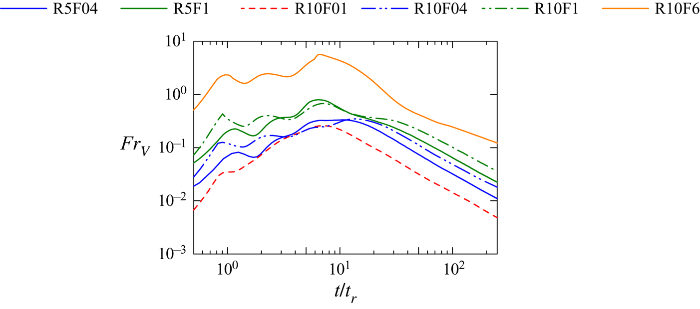
Figure 10. Temporal evolutions of vertical Froude number  $Fr_V$ at $y/M=0$.
4.2. Decay properties of temporally evolving, stably stratified grid turbulence
The decay of temporally evolving grid turbulence is compared with the theories for Saffman and Batchelor turbulence. The velocity and length scales considered in § 2 are defined as
 \begin{equation} U_{H} = (\langle u'^2\rangle + \langle v'^2\rangle)/2,\quad L_{H} = (L_{uH} + L_{vH})/2,\quad L_{V} = (L_{uV} + L_{vV})/2, \end{equation}
where the horizontal and vertical integral scales of each velocity component are defined as
 $$\begin{gather} L_{uH}=\int \frac{\langle u'(x,y,z)u'(x+r_x,y,z)\rangle}{\langle {u'}^2\rangle} {\rm d} r_x,\quad L_{vH} =\int \frac{\langle v'(x,y,z)v'(x,y+r_y,z)\rangle}{\langle {v'}^2\rangle} {\rm d} r_y, \end{gather}$$
 $$\begin{gather}L_{uV}=\int \frac{\langle u'(x,y,z)u'(x,y,z+r_z)\rangle}{\langle {u'}^2\rangle} {\rm d} r_z,\quad L_{vV} =\int \frac{\langle v'(x,y,z)v'(x,y,z+r_z)\rangle}{\langle {v'}^2\rangle} {\rm d} r_z. \end{gather}$$
These statistics depend on  $y$ and $t$. Hereafter, the results are presented only for $y/M=0$ because the statistics are homogeneous during the decay for which the DNS results are compared with the theories.
Time independence of  $U_{H}^2 L_H^4 L_V$ and $U_{H}^2 L_H^2 L_V$ considered in § 2 is derived by the assumption of ‘partial self-similarity’, which means the self-similarity for scales of the order of integral scales (Davidson Reference Davidson2010). If the partial self-similarity is applied, the autocorrelation functions in (4.4a,b) and (4.5a,b) are functions of the separation distance normalized by the integral scale, e.g. $r_x/L_{uH}$. The assumption of the partial self-similarity is examined with the autocorrelation functions of $u$, which are denoted by $f_{uH}(r_x,y,t)=\langle u'(x,y,z,t)u'(x+r_x,y,z,t)\rangle /\langle u'^{2}\rangle$ and $f_{uV}(r_z,y,t)=\langle u'(x,y,z,t)u'(x,y,z+r_z,t)\rangle /\langle u'^{2}\rangle$. Figure 11 plots $f_{uH}$ and $f_{uV}$ at $y=0$ as functions of $r_x/L_{uH}$ and $r_z/L_{uV}$, respectively, in R10F01. For $t/t_r=10$ and 20, the profiles of $f_{uH}$ vary with time. Similarly, $f_{uV}$ is slightly different between $t/t_r=10$ and later times. However, the curves collapse well at later times, and $f_{uH}$ and $f_{uV}$ are functions of $r_x/L_{uH}$ and $r_z/L_{uV}$, respectively, which do not depend on time. The results suggest that the partial self-similarity for large scales is valid except for a very early time.
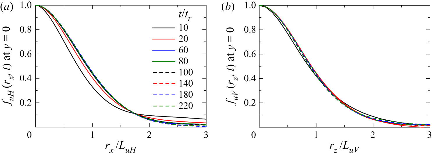
Figure 11. Temporal evolutions of the autocorrelation functions of streamwise velocity defined with separation distances in (a) the streamwise direction,  $r_x$, and (b) the vertical direction, $r_z$. The results are taken at $y=0$ for R10F01. The distance is normalized by the integral scale, $L_{uH}$ or $L_{uV}$.
Saffman turbulence and Batchelor turbulence have a three-dimensional energy spectrum with  $E(k)\sim k^2$ and $k^4$ at large scales, respectively. Axisymmetric turbulence, such as homogeneous turbulence subject to stable stratification or rotation, also has these spectral shapes for Saffman turbulence and Batchelor turbulence. The spectrum in temporally evolving grid turbulence is evaluated with a spherical-shell average following Valente, da Silva & Pinho (Reference Valente, da Silva and Pinho2016). The Fourier transform is applied to the instantaneous velocity $u_{i}(x,y,z,t)$ in the $x$,
$x$,  $y$ and $z$ directions to obtain the Fourier coefficient $\hat {u}_{i}(k_x,k_y,k_z,t)$. The energy spectrum is computed as
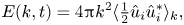 \begin{equation} E(k,t)=4{\rm \pi} k^2\langle \tfrac{1}{2} \hat{u}_{i}\hat{u}_{i}^{*}\rangle_{k},\end{equation}
where  $\hat {u}_{i}^{*}$ is the complex conjugate of $\hat {u}_{i}$, $k$ is the wavenumber and the spherical-shell average $\langle\, f\rangle _{k}$ of $f(k_x, k_y, k_z)$ is defined as
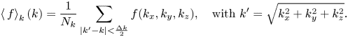 \begin{equation} \left\langle\, f \right\rangle_{k}(k)=\frac{1}{N_k} \sum_{|k'-k|<\frac{\Delta k}{2}} f(k_x, k_y, k_z),\quad \text{with } k'=\sqrt{k_x^2+ k_y^2+k_z^2}. \end{equation}
Here, the summation is taken for  $N_k$ Fourier coefficients whose wavenumber $k'$ satisfies $|k'-k|<\Delta k/2$. The shell thickness is set to be $\Delta k = 0.296M^{-1}$, which is about 1.4 times larger than the wavenumber of the horizontal domain size $2{\rm \pi} /L_x=0.209M^{-1}$.
Figure 12 shows  $E(k)$ of the initial velocity field, where the mean velocity profile is given by (3.5). The wavenumber corresponding to the mesh size $M$ is $k_M=2{\rm \pi} /M$. The inset shows $E(k)$ at a low-wavenumber range. Here, $E(k)$ has distinct peaks at wavenumbers related to $M$, namely $k=k_M$, $2k_M$, $3k_M$ and $4k_M$. The initial velocity field is laminar and does not have the energy spectrum of turbulence, such as $E(k)\sim k^2$ and $k^4$, which can be formed only after the grid turbulence is generated.
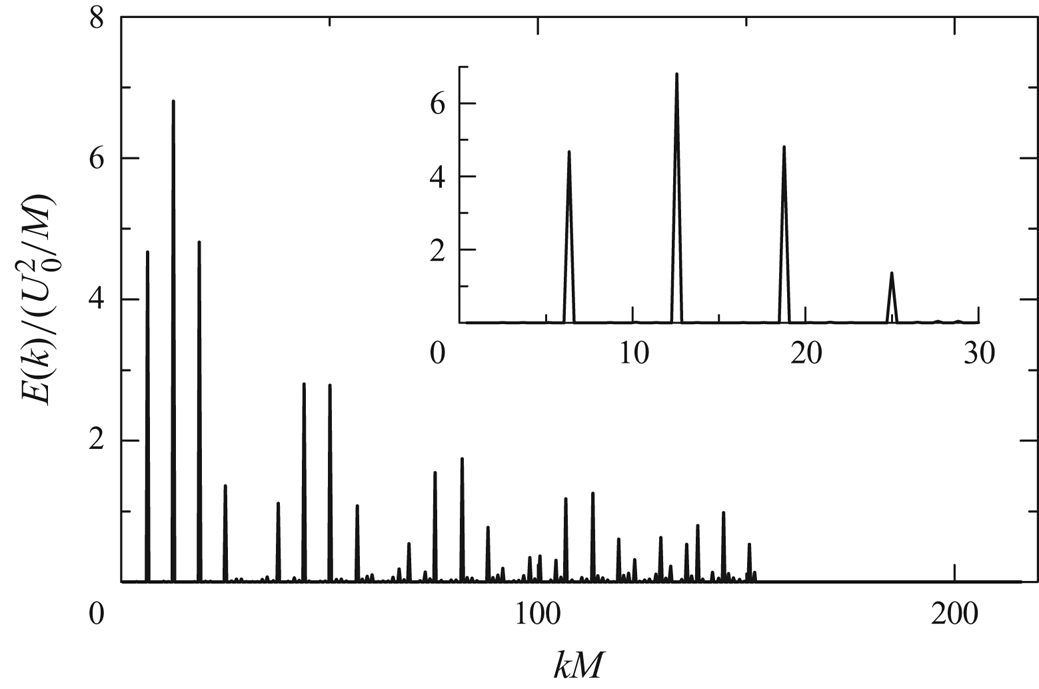
Figure 12. A three-dimensional energy spectrum  $E(k)$ at $t=0$.
The analysis of the turbulent kinetic energy budget suggests that homogeneous turbulence has developed at  $t_H/t_r=12$–33, as summarized in table 1. The energy spectrum after $t/t_r=30$ is examined for the lowest and highest $Fr_M$ cases. Figure 13 shows the temporal evolutions of $E(k)$ for R10F01 and R10F6, which are compared with $E(k)\sim k^2$ and $k^4$. The oscillation of $E(k)$ is due to statistical convergence because $E(k)$ is evaluated from a single snapshot and small $\Delta k$ is used to examine $E(k)$ at large scales. For both cases, $E(k)$ for $kM\lesssim 3$ tends to follow $E(k)\sim k^2$ rather than $E(k)\sim k^4$. As turbulence decays with time, $E(k)$ at high wavenumbers becomes small. However, $E(k)$ at low wavenumbers hardly decay with time, suggesting that a coefficient $A$ in $E(k)\approx Ak^2$ is almost independent of time. The time independence of $A$ is related to the linear momentum conservation, which leads to the invariance of the Saffman integral (Davidson Reference Davidson2013). Therefore, temporally evolving grid turbulence in a stably stratified fluid evolves following the theory of axisymmetric Saffman turbulence. These results suggest that the mean velocity profile (3.5) results in the formation of Saffman turbulence with $E(k)\sim k^2$ in a stably stratified fluid.

Figure 13. Temporal evolutions of the three-dimensional energy spectrum  $E(k)$ for (a) R10F01 and (b) R10F6. The thin black lines represent $E(k)\sim k^2$ and $k^4$.
The invariants of Saffman and Batchelor turbulence are examined in figure 14, which presents the temporal evolutions of  $U_{H}^{2}L_{H}^{2}L_V$ and $U_{H}^{2}L_{H}^{4}L_V$ at $y/M=0$. Once the turbulence is generated, $U_{H}^{2}L_{H}^{2}L_V$ hardly varies while $U_{H}^{2}L_{H}^{4}L_V$ increases with time. Experiments of non-stratified grid turbulence also observed that the invariant of Saffman turbulence, $U^{2}L^{3}$, hardly varies with the distance from the grid while the invariant of the Batchelor turbulence, $U^{2}L^{5}$, monotonically increases as the turbulence decays (Krogstad & Davidson Reference Krogstad and Davidson2010; Kitamura et al. Reference Kitamura, Nagata, Sakai, Sasoh, Terashima, Saito and Harasaki2014). These tendencies agree with the results for $U_{H}^{2}L_{H}^{2}L_V$ and $U_{H}^{2}L_{H}^{4}L_V$ defined for axisymmetric Saffman and Batchelor turbulence. Most wind-tunnel experiments of grid turbulence used conventional square grids, which consist of vertical and horizontal bars while this study considers the rake of vertical plates (Fincham et al. Reference Fincham, Maxworthy and Spedding1996; Praud et al. Reference Praud, Fincham and Sommeria2005). The time independence of $U_{H}^{2}L_{H}^{2}L_V$ indicates that grid turbulence generated by the vertical grid behaves as Saffman turbulence similarly to square-grid turbulence. Comparison of different DNS indicates that $U_{H}^{2}L_{H}^{2}L_V$ becomes independent of time sooner for smaller $Fr_M$. The turbulent kinetic energy budget in figure 8 also suggests a faster transition to homogeneous turbulence for smaller $Fr_M$. These results imply that $U_{H}^{2}L_{H}^{2}L_V=\mathrm {Const}.$ is achieved after the grid turbulence begins to freely decay without the production of turbulent kinetic energy.
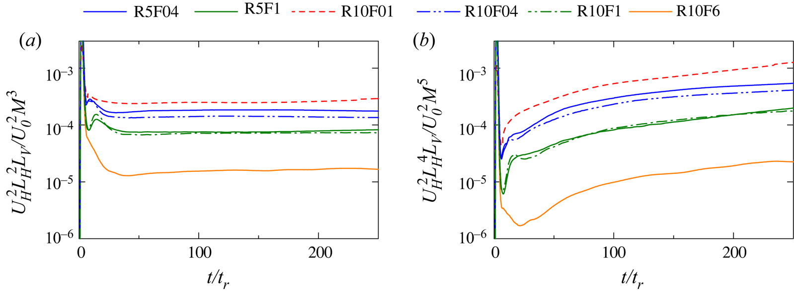
Figure 14. Temporal evolutions of (a)  $U_{H}^{2}L_{H}^{2}L_V$ and (b) $U_{H}^{2}L_{H}^{4}L_V$ at $y/M=0$.
Figure 15(a) presents the temporal variation of the non-dimensional dissipation rate  $\alpha =\varepsilon /(U_H^3/L_H)$, which is assumed to be a constant of order 1 in the derivation of the decay laws in § 2. After $t/t_r\gtrsim 30$, $\alpha$ hardly varies with time except for R10F6. Although $\alpha$ for R10F6 decreases after it attains the peak, $\alpha \approx 0.85$ tends to be constant for $t/t_r\gtrsim 100$. Although $\alpha$ hardly varies with time in each condition, the values of $\alpha$ depend on $Re_M$ and $Fr_M$. Therefore, $\alpha$ is not a universal constant in stratified grid turbulence at low $Re_b$. The values of $\alpha$ for $Fr_M=0.4$ and 1 slightly depend on $Re_M$, and $\alpha$ is slightly larger for $Re_M=5000$. This tendency agrees with DNS of decaying, stably stratified, homogeneous turbulence initialized with a prescribed energy spectrum, where the stationary values of $\alpha$ are larger for lower-Reynolds-number cases (Maffioli & Davidson Reference Maffioli and Davidson2016). As explained in § 2, $\varepsilon =\alpha (U_H^3/L_H)$ for low $Re_b$ is derived with $\varepsilon \sim \nu U_H^2/L_V^2$ and $L_V \sim (\nu L_H/U_H)^{1/2}$. As there are no reasons for prefactors $A$ and $B$ in $\varepsilon =A\nu U_H^2/L_V^2$ and $L_V =B(\nu L_H/U_H)^{1/2}$ to be universal constants which do not depend on flows, $\alpha =A/B^2$ should not be considered as a universal constant. Small temporal variations of $\alpha$ imply that these scalings, $\varepsilon \sim \nu U_H^2/L_V^2$ and $L_V \sim (\nu L_H/U_H)^{1/2}$, are valid during the decay. The decay laws in § 2 are derived based on these scalings, which are satisfied by the power laws in (2.19a–d) and (2.20a–d). The results presented below will also show that the temporal evolutions of $U_H$, $L_H$, $L_V$ and $\varepsilon$ agree with the decay laws of low- $Re_b$ Saffman turbulence except for R10F6, for which $\alpha$ becomes time independent only at a late time. Figure 15(b) shows the relationship between $\alpha$ and $Re_b$. Although $Re_b$ decreases with time, $\alpha$ weakly depends on time. As the flow is not in a strongly stratified turbulence regime, the scaling $\varepsilon \sim U_H^3/L_H$ requires the low- $Re_b$ scaling for $L_V$ and $\varepsilon$. Therefore, $\alpha$ tends to be time independent only when $Re_b$ is small. However, $\alpha$ in R10F01 varies with time even for $0.1\lesssim Re_b \lesssim 0.7$. In this range of $Re_b$, $\alpha$ for other cases varies slowly with $Re_b$. Filled circles in the figure mark $t=t_H$, before which the flow is statistically inhomogeneous. The time independence of $\alpha$ for R10F01 is achieved only after $t=t_H$. Therefore, $\alpha \approx$ Const. also requires the development of grid turbulence, and $\varepsilon \sim U_H^3/L_H$ seems invalid in the wake of each vertical plate.
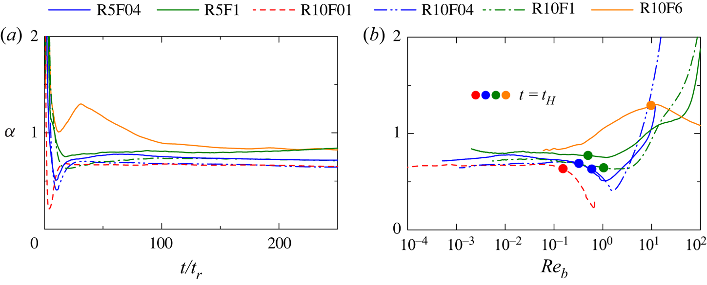
Figure 15. (a) Temporal evolutions of non-dimensional energy dissipation rate  $\alpha =\varepsilon / (U_H^3/L_H)$ at $y/M=0$; (b) $\alpha$ plotted as a function of $Re_b$ at $y/M=0$. The time after $Re_b$ reaches a peak is shown in (b).
The dissipation scaling in non-stratified turbulence can be written as  $\varepsilon =C_\varepsilon (U^3/L)$ with the r.m.s. velocity fluctuations $U$ and integral length scale $L$. The DNS of statistically steady isotropic turbulence has suggested that $C_\varepsilon =\varepsilon /(U^3/L)$ is a universal constant at a high Reynolds number (Ishihara, Gotoh & Kaneda Reference Ishihara, Gotoh and Kaneda2009). However, recent studies have confirmed that $C_\varepsilon$ differs depending on flows even at high $Re$ (Vassilicos Reference Vassilicos2015). Direct numerical simulations and experiments suggest that $C_\varepsilon$ may vary depending on large-scale flow characteristics (Mazellier & Vassilicos Reference Mazellier and Vassilicos2008; Goto & Vassilicos Reference Goto and Vassilicos2016; Takamure et al. Reference Takamure, Sakai, Ito, Iwano and Hayase2019). Large scales of stratified turbulence should be strongly influenced by the Froude number. For example, pancake-like large-scale vortices are often observed in stratified turbulence (Godoy-Diana et al. Reference Godoy-Diana, Chomaz and Billant2004). The dependence of large scales on $Re_M$ and $Fr_M$ can result in variations of $\alpha$. Furthermore, wind-tunnel experiments of active-grid turbulence indicate that $C_\varepsilon$ are different depending on the grid geometry, the operation mode of the active grid and the Reynolds number, although $C_\varepsilon$ in each experiment hardly varies with the decay of turbulence (Mora et al. Reference Mora, Pladellorens, Turró, Lagauzere and Obligado2019; Zheng, Nagata & Watanabe Reference Zheng, Nagata and Watanabe2021b). This behaviour is similar to the evolution of $\alpha$ in figure 15(a) since $\alpha$ in a late time weakly depends on time but differs depending on $Re_M$ and $Fr_M$. Although the underlying assumption is different for $\varepsilon = C_\varepsilon U^3/L$ in non-stratified turbulence and $\varepsilon = \alpha U_H^3/L_H$ in stratified turbulence, these previous studies of non-stratified turbulence imply that $\alpha$ does not have to be a universal constant.
In all DNS the flow reaches the viscosity-affected stratified regime during the decay and  $\alpha$ hardly varies with time at a late time. Furthermore, $U_{H}^{2}L_{H}^{2}L_V$ also hardly depends on time as suggested from the theory of Saffman turbulence. In the rest of the paper, the decay properties are compared with the theoretical results of low- $Re_b$ Saffman turbulence presented in § 2. First, we briefly discuss the decay of main variables and then provide detailed discussions on the decay exponents based on least square estimation.
Figure 16(a) examines the decay of  $U_H^2$, which is compared with the power law $U_H^2\sim t^{-5/4}$. The slope of $U_H^2$ is close to the $-5/4$th law except for R10F6. The decay of $U_H^2$ for R10F6 is slightly slower than $U_H^2\sim t^{-5/4}$ even for $t/t_r\geq 100$, for which the assumptions of constant values of $\alpha$ and $U_H^2L_H^2L_V$ are valid. Then, the deviation from $U_H^2\sim t^{-5/4}$ should be attributed to the validity of (2.18), which may not be valid when $Fr_M$ is not sufficiently low. It is also clear that the decay exponent of R10F6 is not constant for $30\lesssim t/t_r\lesssim 100$ because $\alpha$ also varies with time, although the grid turbulence has fully developed by $t/t_r=30$. Figure 16(b) shows the variation of the kinetic energy dissipation rate $\varepsilon$. As expected for Saffman turbulence with low $Re_b$, the present DNS results with $Fr_M\leq 1$ follow $\varepsilon \sim t^{-9/4}$ during the decay.
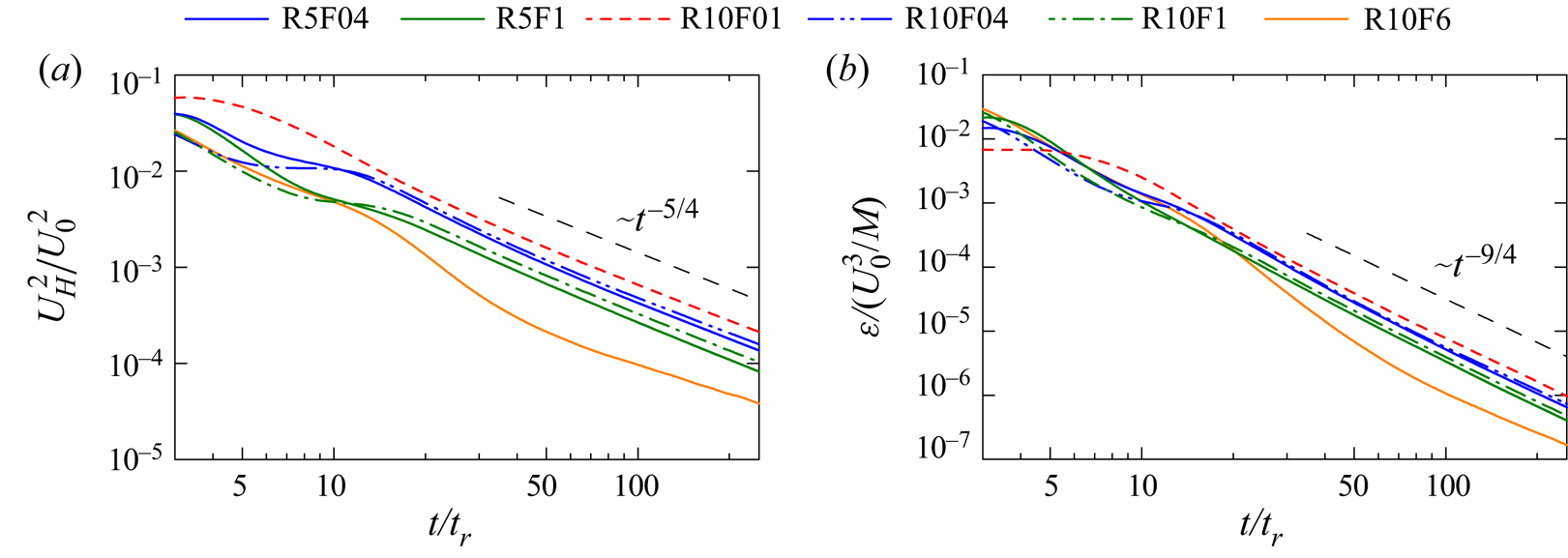
Figure 16. Decay of (a) horizontal velocity fluctuations  $U_H^2$ and (b) turbulent kinetic energy dissipation rate $\varepsilon$ at $y/M=0$.
Figure 17(a,b) shows the variations of integral scales,  $L_H$ and $L_V$. The $Re_M$ dependence is weak for $L_H$, which is more dependent on $Fr_M$. The increase of $L_H$ follows $L_H\sim t^{3/8}$ from $t/t_r\approx 20$ except for R10F6, for which $L_H\sim t^{3/8}$ is valid only after $t/t_r\approx 100$. Although $L_V$ depends on both $Re_M$ and $Fr_M$ at an early time, it hardly depends on $Re_M$ at a late time as the lines for different $Fr_M$ converge to a single line. The DNS results with $Fr_M\leq 1$ follow $L_V\sim t^{1/2}$. However, $L_V\sim t^{1/2}$ tends to prevail at a later time than $L_H\sim t^{3/8}$ especially for higher $Fr_M$. For R10F6, the exponent is different from 1/2 even at the end of the simulation.
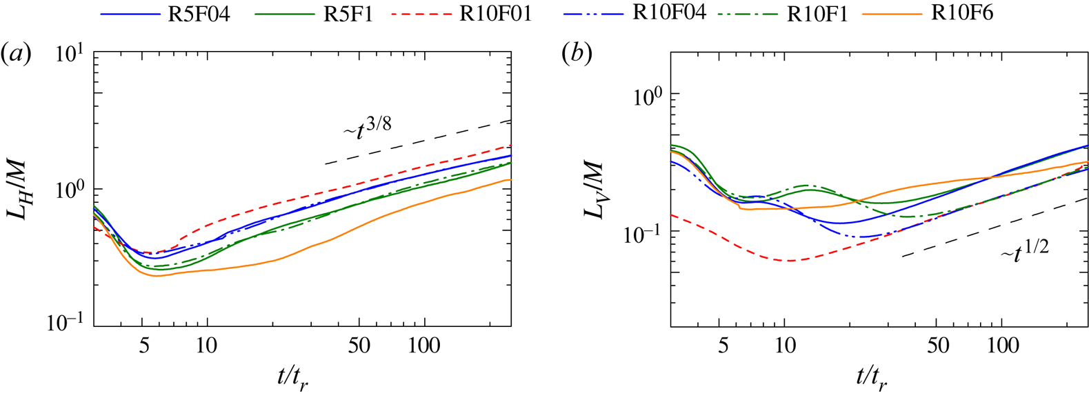
Figure 17. Temporal evolutions of (a) horizontal and (b) vertical integral length scales at  $y/M=0$.
Turbulence is initially generated as turbulent wakes, whose interaction results in the formation of grid turbulence. Therefore, the flow behaviour at an early time can be related to that of stably stratified turbulent wakes. For an axisymmetric wake generated by a sphere or a disk, the characteristic length of large scales is often defined with the spatial distribution of mean velocity deficit or turbulent kinetic energy (Diamessis et al. Reference Diamessis, Spedding and Domaradzki2011; Chongsiripinyo & Sarkar Reference Chongsiripinyo and Sarkar2020). The DNS of the stably stratified wake of a disk shows that both horizontal and vertical length scales slightly decrease when the turbulent wake is being generated (Chongsiripinyo & Sarkar Reference Chongsiripinyo and Sarkar2020). Once the wake becomes turbulent, these length scales increase as the wake evolves. These evolutions of the length scales are similar in figure 17, and the wake length scales defined with mean velocity or turbulent kinetic energy can be related to the integral scales defined with the autocorrelation functions of horizontal velocity.
Figure 18(a) examines the decay of potential energy  $E_P$. The present DNS results exhibit wave-like oscillations of $E_P$, as also found in previous DNS (de Bruyn Kops & Riley Reference de Bruyn Kops and Riley2019). This can be confirmed from the inset of figure 18(a), where $E_P$ between $t/t_r=105$ and 107 is shown for R10F01 in a linear plot. However, the amplitude of the oscillation is much smaller than the variation of $E_P$ during the decay, for which $E_P$ decreases from $E_P/U_0^2={{O}}(10^{-3})$ to ${{O}}(10^{-8})$. Therefore, the wave-like oscillation of $E_P$ is not visible in the logarithmic plot and does not affect the overall decay rate of $E_P$. The decay for $Fr_M=0.1$ and 0.4 tends to follow the power law of $E_P\sim t^{-7/2}$. However, a deviation from $E_P\sim t^{-7/2}$ is found for $Fr_M=0.4$ after $t/t_r\approx 150$. The power law $E_P\sim t^{-7/2}$ assumes (2.15) and (2.18), which can be used to derive $E_P/k_H \sim Re_b$ for the ratio of $E_P$ to the horizontal kinetic energy $k_H=U_H^2$. Figure 18(b) plots the relation between $Re_b$ and $E_P/k_H$ after $Re_b$ reaches a peak. The present DNS results are compared with the DNS of forced, stably stratified homogeneous turbulence in Brethouwer et al. (Reference Brethouwer, Billant, Lindborg and Chomaz2007). Below $Re_b\approx 10$, $E_P/k_H$ decreases with $Re_b$ being small. The ratio $E_P/k_H$ for $Fr_M=0.1$ tends to follow $E_P/k_H \sim Re_b$ for $Re_b\lesssim 10^{-1}$. Although this relation is found for $Re_b\approx 10^{-2}$ in the cases of $Fr_M=0.4$, the DNS data deviate from $E_P/k_H\sim Re_b$ at a lower $Re_b$. For R10F01, $E_P/k_H\sim Re_b$ is valid for a wide range of $Re_b$ and, therefore, the decay of $E_P$ approximately follows $E_P\sim t^{-7/2}$.
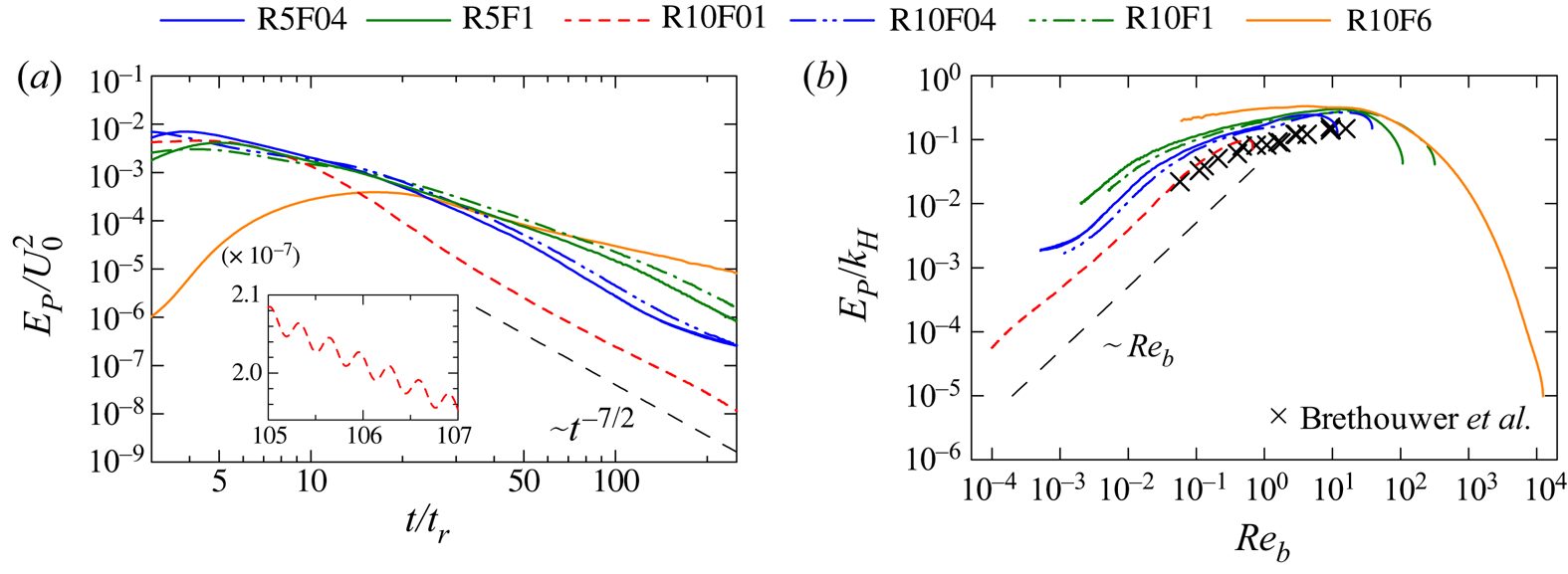
Figure 18. (a) Decay of potential energy  $E_P$ at $y/M=0$. (b) The buoyancy Reynolds number dependence of the ratio between the potential and horizontal kinetic energies $E_P/k_H$. The trajectory in $(Re_b,E_P/k_H)$ space at $y/M=0$ is shown after $Re_b$ reaches a peak. Direct numerical simulation results of forced, stably stratified homogeneous turbulence are also shown for comparison (Brethouwer et al. Reference Brethouwer, Billant, Lindborg and Chomaz2007).
Although the discussion in § 2 does not provide the decay law of the potential energy dissipation rate  $\varepsilon _P$, the decay law in a form of $\varepsilon _P\sim t^{n}$ may be empirically established because the ratio $\varepsilon _P/\varepsilon$ often depends on $Re_b$ (Brethouwer et al. Reference Brethouwer, Billant, Lindborg and Chomaz2007). Figure 19(a) shows the relation between $Re_b$ and $\varepsilon _P/\varepsilon$, which is compared again with DNS by Brethouwer et al. (Reference Brethouwer, Billant, Lindborg and Chomaz2007). For $Re_b\gtrsim 10^{-1}$, the variation of $\varepsilon _P/\varepsilon$ with $Re_b$ is consistent between decaying grid turbulence and forced homogeneous turbulence. For $Re_b\lesssim 10^{-1}$, $\varepsilon _P/\varepsilon$ decreases as $Re_b$ becomes small. The present data roughly follows $\varepsilon _P/\varepsilon \sim Re_b$ for $Re_b\lesssim 10^{-2}$. This relation $\varepsilon _P\sim \varepsilon Re_b=\varepsilon ^{2}/N^2\nu$ combined with the decay laws of $\varepsilon$ in (2.19a–d) and (2.20a–d) yields
 $$\begin{gather} \varepsilon_P\sim t^{{-}9/2}\quad \text{for low-}Re_b\ \text{Saffman turbulence}, \end{gather}$$
 $$\begin{gather}\varepsilon_P\sim t^{{-}5}\quad \text{for low-}Re_b\ \text{Batchelor turbulence}. \end{gather}$$
An alternative way to derive these decay laws is neglecting the buoyancy flux term in (2.7), and  ${\rm d} E_P/{\rm d} t=-\varepsilon _P$ with (2.21) and (2.22) yields (4.8) and (4.9), respectively. Indeed, the wave-like oscillation of $E_P$ arising from the buoyancy flux was shown to be smaller than the overall decay of $E_P$ in figure 18(a). Figure 19(b) compares the decay of $\varepsilon _P$ with $\varepsilon _P\sim t^{-9/2}$. The present DNS data except for R10F6 follows $\varepsilon _P\sim t^{-9/2}$ derived based on the empirical relation $\varepsilon _P\sim \varepsilon Re_b$ combined with the decay law of Saffman turbulence.
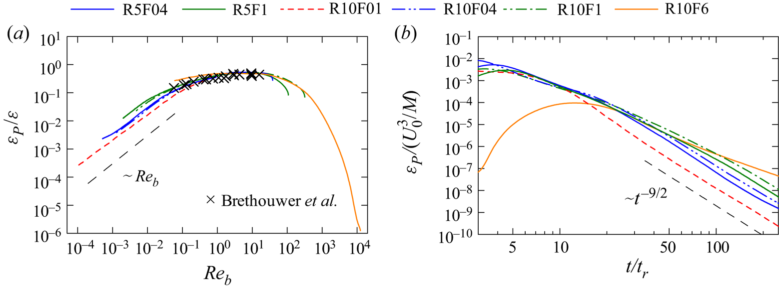
Figure 19. (a) The buoyancy Reynolds number dependence of the ratio between the dissipation rates of potential energy and kinetic energy  $\varepsilon _P/\varepsilon$. The results are shown after the peak of $Re_b$. Direct numerical simulation results of forced, stably stratified homogeneous turbulence are also shown for comparison (Brethouwer et al. Reference Brethouwer, Billant, Lindborg and Chomaz2007). (b) Decay of potential energy dissipation rate $\varepsilon _P$. All results are taken at $y/M=0$.
It should be noted that  $\varepsilon _P\sim \varepsilon Re_b$ is valid only when $Re_b$ is sufficiently small. Figure 19(a) suggest that $\varepsilon _P/\varepsilon$ weakly depends on $Re_b$ for $1\lesssim Re_b \lesssim 10$. Strong $Re_b$-dependence of $\varepsilon _P/\varepsilon$ is observed for $Re_b\gtrsim 10^1$. This range of $Re_b$ is in the production phase of grid turbulence and the grid turbulence has not fully developed yet. Brethouwer et al. (Reference Brethouwer, Billant, Lindborg and Chomaz2007) also observed that $\varepsilon _P/\varepsilon =0.4$– $0.5$ hardly depends on $Re_b$ when $Re_b\sim Re_HFr_H^2>1$. Similar values of $\varepsilon _P/\varepsilon$ were also reported by Riley & de Bruyn Kops (Reference Riley and de Bruyn Kops2003), Lindborg (Reference Lindborg2006) and Maffioli & Davidson (Reference Maffioli and Davidson2016). If $\varepsilon _P/\varepsilon$ is constant during the decay, the decay exponent of $\varepsilon _P$ is the same as that of $\varepsilon$. The relation $\varepsilon _P\sim \varepsilon$ might be useful at a high- $Re_b$ regime, for which one can derive, from (2.13a–d) and (2.14a–d), the following decay laws of $\varepsilon _P$:
 $$\begin{gather} \varepsilon_P\sim t^{{-}9/5}\quad \text{for high-}Re_b\ \text{Saffman turbulence}, \end{gather}$$
 $$\begin{gather}\varepsilon_P\sim t^{{-}15/7}\quad \text{for high-}Re_b \text{Batchelor turbulence}. \end{gather}$$
However, the Reynolds number is not large enough in the present DNS to verify these decay laws.
One of the important parameters in oceanography is mixing efficiency that is often defined as  $\eta _{mix}=\varepsilon _P/(\varepsilon +\varepsilon _P)=(1+ \varepsilon /\varepsilon _P)^{-1}$ (Smyth, Moum & Caldwell Reference Smyth, Moum and Caldwell2001; Gregg et al. Reference Gregg, D'Asaro, Riley and Kunze2018). The DNS of stably stratified turbulence has been utilized to parametrize $\eta _{mix}$ (Salehipour, Peltier & Mashayek Reference Salehipour, Peltier and Mashayek2015; Maffioli, Brethouwer & Lindborg Reference Maffioli, Brethouwer and Lindborg2016; de Bruyn Kops & Riley Reference de Bruyn Kops and Riley2019; VanDine, Pham & Sarkar Reference VanDine, Pham and Sarkar2021). If $\varepsilon _P/\varepsilon$ is constant during the decay, $\eta _{mix}$ does not vary with time. However, the decay laws derived for low- $Re_b$ Saffman and Bachelor turbulence suggest that $\eta _{mix}$ decays with time as $\eta _{mix}\sim (1+A_\eta t^{9/4})^{-1}$ for Saffman turbulence and $\eta _{mix}\sim (1+A_\eta t^{5/2})^{-1}$ for Batchelor turbulence. As long as the late time behaviour of grid turbulence is concerned, we may approximate these decay laws as
 $$\begin{gather} \eta_{mix} \sim t^{{-}9/4}\quad \text{for low-}Re_b\ \text{Saffman turbulence}, \end{gather}$$
 $$\begin{gather}\eta_{mix} \sim t^{{-}5/2}\quad \text{for low-}Re_b\ \text{Batchelor turbulence}. \end{gather}$$
 Figure 20 shows the temporal variation of  $\eta _{mix}$ compared with (4.12). As expected, $\eta _{mix}$ decreases as turbulence decays. Before the decay of $\eta _{mix}$ begins, $\eta _{mix}$ is about $0.33$, which is close to the values corresponding to $\varepsilon _P/\varepsilon =0.4$– $0.5$ and is consistent with other DNS studies of stratified homogeneous turbulence (de Bruyn Kops & Riley Reference de Bruyn Kops and Riley2019). The decay of $\eta _{mix}$ tends to follow (4.12), although $\eta _{mix} \sim t^{-9/4}$ is observed at a later time for higher $Fr_M$. de Bruyn Kops & Riley (Reference de Bruyn Kops and Riley2019) also found in DNS of decaying, stably stratified homogeneous turbulence that $\eta _{mix}$ stays at an almost constant value at an early time of the decay with high $Re_b$ and then decreases with time once $Re_b$ becomes small, although this decay was not emphasized in their paper.
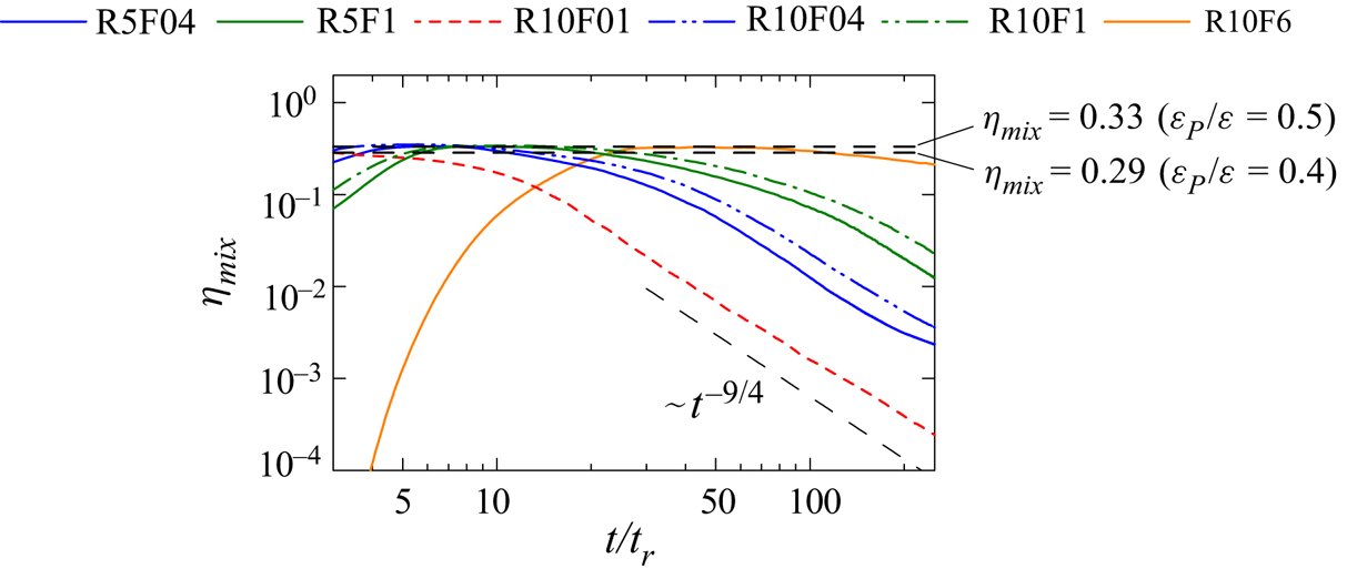
Figure 20. Temporal variation of mixing efficiency  $\eta _{mix}=\varepsilon _P/(\varepsilon +\varepsilon _P)$ at $y/M=0$. Horizontal broken lines represent $\eta _{mix}$ with $\varepsilon _P/\varepsilon =0.4$ and 0.5.
Figure 21 shows the decay of vertical velocity variance  $\langle w'^2\rangle$. The theories for stably stratified turbulence in § 2 concerns large-scale characteristics of the flow and do not provide the decay law of $\langle w'^2\rangle$, which is dominated by small-scale fluctuations in stratified turbulence. However, $\langle w'^2\rangle$ tends to follow $\langle w'^2\rangle \sim t^{-1}$ except for R10F6. Towed-grid experiments by Praud et al. (Reference Praud, Fincham and Sommeria2005) also observed $\langle w'^2\rangle \sim t^{-1}$ at low $Fr_M$.
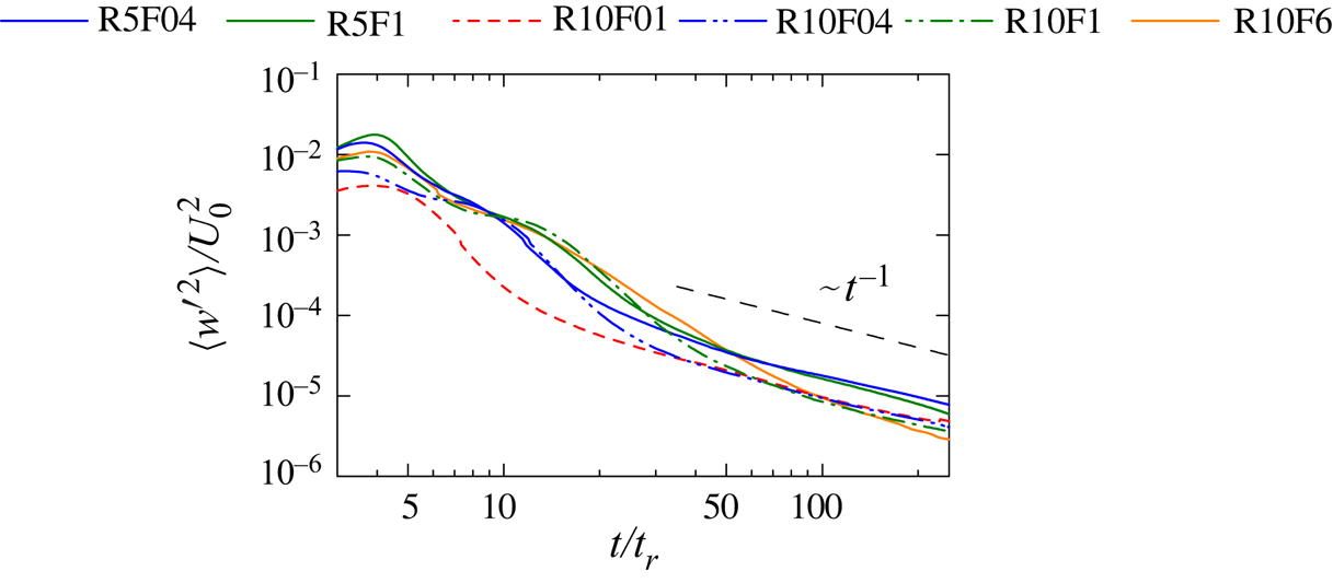
Figure 21. Decay of vertical velocity variance  $\langle w'^2\rangle$ at $y/M=0$.
These results suggest that temporally evolving grid turbulence in a stratified fluid behaves similarly to Saffman turbulence. Previous numerical studies of Saffman turbulence and Batchelor turbulence consider decaying turbulence initialized with a velocity field that satisfies  $E(k)\sim k^2$ or $k^4$ at large scales (Ishida, Davidson & Kaneda Reference Ishida, Davidson and Kaneda2006; Teitelbaum & Mininni Reference Teitelbaum and Mininni2012; Yoshimatsu & Kaneda Reference Yoshimatsu and Kaneda2018; de Bruyn Kops & Riley Reference de Bruyn Kops and Riley2019; Anas et al. Reference Anas, Joshi and Verma2020). It has been shown that the decay of turbulence with the $k^2$ and $k^4$ spectra is consistent with the theories of Saffman and Batchelor turbulence, respectively. However, these studies do not reveal how turbulence with $E(k)\sim k^2$ or $k^4$ is generated because the energy spectrum is imposed as the initial condition. The temporally evolving grid turbulence is initialized with a laminar flow that approximates the mean velocity deficit of the wakes. Therefore, the production of turbulence occurs simply due to the mean velocity gradient imposed as the initial condition. The results presented above imply that the mean velocity deficit caused by the grid is essential for grid turbulence to behave like Saffman turbulence.
4.3. Estimation of decay exponents
The results shown above indicate that most quantities vary with time in accord with a power law of  $t$. From experiments and numerical simulations of grid turbulence with and without stable stratification, it is widely accepted that the decay of horizontal velocity fluctuations follows
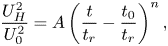 \begin{equation} \frac{U_H^2}{U_0^2}=A\left(\frac{t}{t_r}-\frac{t_0}{t_r}\right)^{n}, \end{equation}
where  $t_0$ is the virtual origin. Various methods have been proposed to determine the unknown parameters $A$,
$A$,  $t_0$ and $n$ from data taken in laboratory experiments of non-stratified grid turbulence (Lavoie et al. Reference Lavoie, Djenidi and Antonia2007; Krogstad & Davidson Reference Krogstad and Davidson2010; Valente & Vassilicos Reference Valente and Vassilicos2011). Most methods provide a similar decay exponent $n$, although small variations may exist because the virtual origin is determined in a different manner. These methods are based on linear or nonlinear least square estimation applied to a certain range of decay. It is known that the fitting range $t_{s} \leq t \leq t_{e}$ may significantly affect $n$ in non-stratified grid turbulence, where $t_{s}$ and $t_{e}$ are the start and end points (time) of the fitting range. As discussed in the introduction, a near-grid region has a faster decay rate than a fully developed turbulence region (Komori et al. Reference Komori, Nagata, Kanzaki and Murakami1993; Krogstad & Davidson Reference Krogstad and Davidson2012). Furthermore, $n$ also increases as turbulence decays to a low-Reynolds-number regime. Here, the variation of $n$ is often explained by that of $C_\varepsilon$. Except for R10Fr6 the temporal variation of $\alpha =\varepsilon /(U_H^3/L_H)$ in figure 15 is large for $t/t_r\lesssim 20$, which may correspond to the non-equilibrium decay region in the case of non-stratified grid turbulence generated by a square grid (Isaza, Salazar & Warhaft Reference Isaza, Salazar and Warhaft2014; Nagata et al. Reference Nagata, Saiki, Sakai, Ito and Iwano2017). Therefore, $t/t_r\lesssim 20$ should be eliminated from the data used to estimate $n$. Furthermore, the power law of $L_V$ predicted for low $Re_b$ seems valid for $t/t_r\gtrsim 20$ for $Fr=0.1$, $t/t_r\gtrsim 30$ for $Fr=0.4$ and $t/t_r\gtrsim 60$ for $Fr=1$ in figure 17(b). By taking these points into consideration, $t_{s}/t_r=70$ is adapted except for R10F6. We have also confirmed that the decay exponents obtained with larger $t_{s}$ hardly differ from those with $t_s/t_r=70$. The assumption of constant $\alpha$ becomes valid only after $t\approx 100$ for R10F6, and $n$ is estimated with $t_s/t_r=120$. In all cases, the fitting range is within the viscosity-affected stratified flow regime. Experiments at very large $t/t_r$ $(x/M)$ often have a difficulty in dealing with background velocity fluctuations that can be comparable to turbulent fluctuations and with measurement errors arising from, for example, electronic noise of hot-wire anemometry. Therefore, the end point of the fitting range has to be carefully determined in experiments. However, these issues do not affect the estimation of $n$ in numerical simulations. Furthermore, the decay of turbulence in a stably stratified fluid does not result in the increase of $\alpha$, which is almost constant even in a late time. The estimation of $n$ in stratified grid turbulence is not as sensitive to $t_e$ as in experiments of non-stratified grid turbulence. Therefore, $t_e$ is set as the end of the computations, i.e. $t_e/t_r=250$.
This study compares  $n$ obtained by three methods explained here. Method 1 predetermines $t_0/t_r$ and applies a linear least square method to the DNS data of $(U_H^2/U_0^2, t/t_r-t_0/t_r)$ in a form of $\ln (U_H^2/U_0^2)=\ln A+ n\ln (t/t_r-t_0/t_r)$, for which $\ln A$ and $n$ are analytically determined. The fitting is repeatedly applied by changing $t_0/t_r$ from $-100$ to $100$ with an increment of $0.1$. The virtual origin $t_0/t_r$ is determined such that the standard deviation of the DNS data from the fitting function is the smallest for all tested virtual origins. This virtual origin is used to determine $\ln A$ and $n$ with the linear least square method. The condition of the minimum standard deviation is often used to determine one of the fitting parameters, e.g. a range of $t$ (or $x$ in wind-tunnel experiments) where the least square method is applied to calculate $n$ (Krogstad & Davidson Reference Krogstad and Davidson2010; Kitamura et al. Reference Kitamura, Nagata, Sakai, Sasoh, Terashima, Saito and Harasaki2014). Method 2 assumes that the virtual origin is equal to zero and the linear least square method is applied for $\ln (U_H^2/U_0^2)=\ln A+ n\ln (t/t_r)$ to determine $\ln A$ and $n$. This method yields the decay exponent equivalent to those considered in some previous studies on stably stratified grid turbulence, where the decay exponent was obtained for $(U_H^2/U_0^2)=A(t/t_r)^{n}$ with the assumption of $t_0=0$ (Liu Reference Liu1995; Praud et al. Reference Praud, Fincham and Sommeria2005; Espa et al. Reference Espa, Avallone and Cenedese2018). Method 3 directly applies a nonlinear least square method (Levenberg–Marquardt method) to simultaneously determine $A$,
$A$,  $t_0/t_r$ and $n$ of (4.14). The nonlinear least square method has been widely used for experimental data of grid turbulence and was shown to provide $n$ consistent with other methods (Valente & Vassilicos Reference Valente and Vassilicos2011; Isaza et al. Reference Isaza, Salazar and Warhaft2014; Kitamura et al. Reference Kitamura, Nagata, Sakai, Sasoh, Terashima, Saito and Harasaki2014; Zheng, Nagata & Watanabe Reference Zheng, Nagata and Watanabe2021a).
Table 2 summarizes the decay exponent and virtual origin obtained by the three methods. Exponent  $n$ for R10F6 is smaller than for the other cases, as also expected from the slower decay of R10F6 in figure 16(a). However, $n$ for $Fr=0.1$, 0.4 and 1 is close to $n=-1.25$ derived for low- $Re_b$ Saffman turbulence. Although each method yields different virtual origins, the estimated values of $n$ differ only slightly. This weak sensitivity of $n$ to the choice of $t_0$ is related to the fitting range that includes large $t/t_r$ up to 250 because the decay exponent estimated from data at large $t/t_r$ is known to be insensitive to small variations of the virtual origin (Zheng et al. Reference Zheng, Nagata and Watanabe2021a). The variations of $n$ found among the three methods are at a similar level to experimental results of non-stratified grid turbulence (Valente & Vassilicos Reference Valente and Vassilicos2011). Averages of $n$ taken except for R10F6 are $-1.20$, $-1.25$ and $-1.23$ for methods 1, 2 and 3, respectively. These values are fairly close to the prediction $n=-1.25$ for low- $Re_b$ Saffman turbulence.
Table 2. Decay exponents and virtual origins estimated by three different methods.
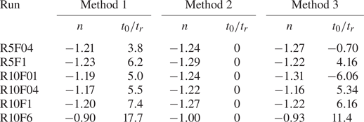
The DNS results suggest that a power law  $f=A(t-t_0)^{n}$ is also valid for various quantities shown in figures 16–19. Exponent $n$ is estimated by applying the linear least square method to $\ln f=\ln A+ n\ln (t-t_0)$ with the virtual origin estimated from $U_H^2$ by method 1. Table 3 summarizes the estimated values of $n$ for the integral scales, potential energy and dissipation rates of kinetic and potential energies. The exponents for $L_H$, $L_V$ and $\varepsilon$ are close to the values for low- $Re_b$ Saffman turbulence except for R10F6. The faster growth of $L_V$ than $L_H$ is also found for DNS data as predicted for low- $Re_b$ Saffman turbulence. The decay of $E_P$ and $\varepsilon _P$ of the DNS data tends to be slower than low- $Re_b$ Saffman turbulence, although the difference from the theory is not large for some cases, e.g. R10F04 and R10F01. This is because the exponents of $E_P/k_H \sim Re_b^{p}$ and $\varepsilon _P/\varepsilon \sim Re_b^{p}$ deviate from $p=1$ especially for large $Re_b$ while $n=-3.5$ for $E_P$ and $-4.5$ for $\varepsilon _P$ require $p=1$.
Table 3. Power-law exponents of integral scales, potential energy and dissipation rates of kinetic and potential energies.
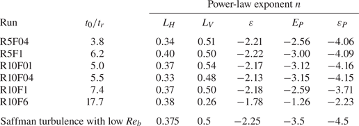
5. Decay properties of stably stratified grid turbulence: a review of experimental data
The present DNS results have confirmed that the decay of temporally evolving, stably stratified grid turbulence is consistent with the theory for low- $Re_b$ Saffman turbulence. It is natural to consider that whether decaying homogeneous turbulence obeys the decay laws of Saffman turbulence or Batchelor turbulence depends on the generation process of turbulence (Davidson Reference Davidson2004). Therefore, it is also important to compare the present findings with experimental data because the temporal grid turbulence is only an approximation of actual grid turbulence studied in laboratories.
Praud et al. (Reference Praud, Fincham and Sommeria2005) presented the measurement results of horizontal kinetic energy and horizontal and vertical integral scales for turbulence generated by a towed rake of vertical plates for  $1125\leq Re_M\leq 36000$ and $0.021\leq Fr_M \leq 0.36$. The parameter ranges of $(Re_M, Fr_M)$ are similar to the present DNS although their Schmidt number is larger than 1 because the experiments were conducted with saltwater. The decay laws of low- $Re_b$ Saffman turbulence are expected for their experiments. Although other experimental studies also investigated stratified grid turbulence for similar values of $(Re_M, Fr_M)$, the number of data points in the plot of $U_H^2$ is not enough to assess the decay rate or the horizontal and vertical integral scales are not available (Itsweire et al. Reference Itsweire, Helland and Van Atta1986; Yap & Van Atta Reference Yap and Van Atta1993; Fincham et al. Reference Fincham, Maxworthy and Spedding1996). Therefore, we present comparisons with low- $Re_b$ Saffman turbulence only for Praud et al. (Reference Praud, Fincham and Sommeria2005). Figure 22 shows temporal variations of $U_{H}^{2}L_{H}^{2}L_V$ and $U_{H}^{2}L_{H}^{4}L_V$ in their experiments, which are constant for Saffman turbulence and Batchelor turbulence, respectively. As also observed in the present DNS, $U_{H}^{2}L_{H}^{2}L_V$ hardly varies with time while $U_{H}^{2}L_{H}^{4}L_V$ increases. Thus, the grid turbulence investigated in their facility also behaves as axisymmetric Saffman turbulence. They also observed that the decay of $U_{H}^{2}$ measured under various conditions follows $U_H^2 \sim t^{-1.3}$, which is close to $t^{-1.25}$ of low- $Re_b$ Saffman turbulence. We estimate the decay exponent of horizontal kinetic energy $U_H^2$ from one of their experiments with $(Re_M, Fr_M)=(9000, 0.086)$, for which $U_H^2$ was measured for $30\lesssim t/t_r \lesssim 150$. We have obtained $n=-1.31$ and $t_0/t_r=8$ for $U_H^2/U_0^2 = A(t/t_r-t_0/t_r)^{n}$ by applying the maximum decay range method (Lavoie et al. Reference Lavoie, Djenidi and Antonia2007). For the same experiment with $(Re_M, Fr_M)=(9000, 0.086)$, we have obtained $L_H\sim (t/t_r-8)^{0.30}$ and $L_V\sim (t/t_r-8)^{0.48}$ with the least square method. Furthermore, they also estimated the kinetic energy dissipation rate $\varepsilon$ based on the gradients of horizontal velocity and found that $\varepsilon$ decays as $\varepsilon \sim t^{-2.3}$. These power-law exponents in their experiments are close to the values of low- $Re_b$ Saffman turbulence. The slower growth of $L_H$ than $L_V$ is also consistent with the theoretical prediction. Thus, their experimental results are explained well by the decay laws derived for low- $Re_b$ Saffman turbulence.
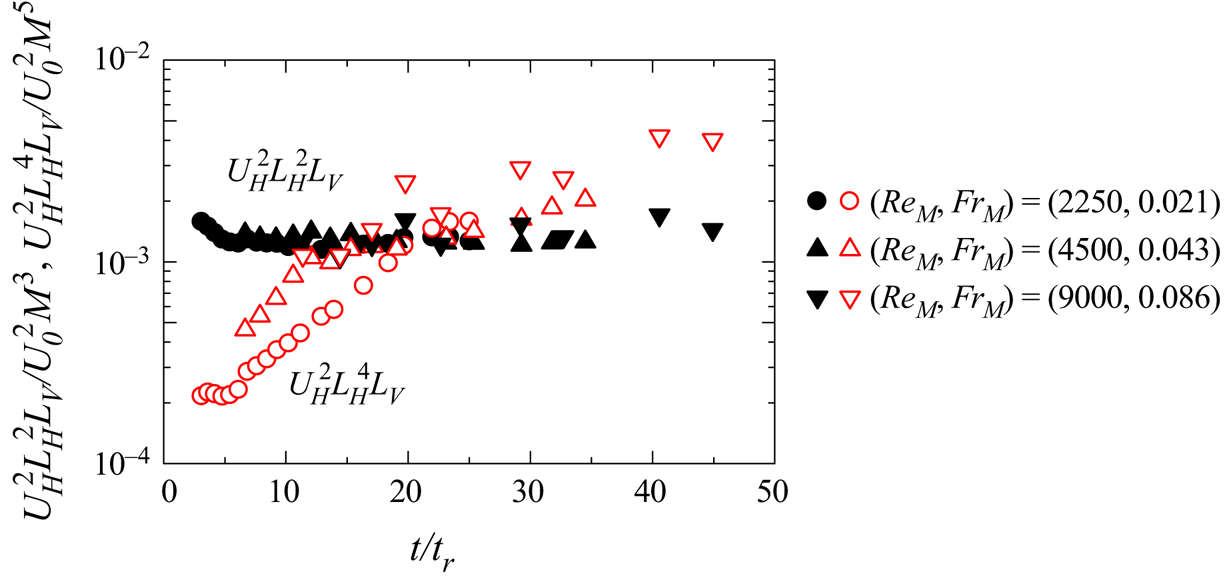
Figure 22. Temporal evolutions of  $U_{H}^{2}L_{H}^{2}L_V$ and $U_{H}^{2}L_{H}^{4}L_V$ in experiments of towed-grid turbulence in Praud et al. (Reference Praud, Fincham and Sommeria2005).
Experiments of stably stratified grid turbulence have also been conducted for higher  $Fr_M$ than Praud et al. (Reference Praud, Fincham and Sommeria2005). Itsweire et al. (Reference Itsweire, Helland and Van Atta1986) presented the measurement results of $U_H^2$ in grid turbulence with $Fr_M\approx 7$–15 in a ten-layer, salt-stratified water channel. They found that the decay of $U_H^2$ in stratified grid turbulence is faster than in non-stratified cases. Similarly, Liu (Reference Liu1995) also reported that the decay becomes faster by the stable stratification in experiments of towed-grid turbulence in a linearly stratified fluid for $Fr_M=40$ and 80. On the other hand, water-channel experiments of grid turbulence with a stable linear density gradient by Stillinger, Helland & Van Atta (Reference Stillinger, Helland and Van Atta1983) observed the opposite effect on $U_H^2$ for $Fr_M\approx 14$–29: the decay becomes slow by the influence of stable stratification. Lienhard & van Atta (Reference Lienhard and van Atta1990) conducted wind-tunnel experiments of thermally stratified grid turbulence with a linear density profile for $Fr_M\approx 17$–42. However, they did not find significant influences of stable stratification on the decay of $U_H^2$. Similarly, for grid turbulence in a two-layer, density-stratified water, Huq & Britter (Reference Huq and Britter1995) and Komori & Nagata (Reference Komori and Nagata1996) reported that the decay rate of $U_H^2$ was hardly influenced by the stable stratification for $Fr_M\approx 3$. These studies observed different influences of stable stratification on the decay of horizontal velocity fluctuations for $Fr_M={{O}}(10^0$– $10^1)$. The present DNS of R10F6 suggests that the decay rate of $U_H^2$ varies with time in figure 16(a), where the least square method yields $U_H^2/U_0^2\sim (t/t_r)^{-2.3}$ for $15\leq t/t_r\leq 40$ and $U_H^2/U_0^2\sim (t/t_r)^{-1}$ at a later time. The Saffman turbulence without density stratification decays as $U_H^2/U_0^2\sim (t/t_r)^{-1.2}$. Thus, the decay rate for $Fr_M=6$ is faster in the early time than for the non-stratified case and slower in the late time, and the decay exponent is not constant during the decay. Furthermore, R10F6 also suggests that the non-dimensional dissipation rate $\alpha$ is not constant in the early time of decay until $t/t_r\approx 100$. The time independence of $\alpha$ is the basis of the power law of $U_H^2$ with a constant exponent $n$. This is possibly related varieties of the stratification influences on the decay reported in previous experiments with $Fr_M={{O}}(10^0$– $10^1)$ because most experiments were conducted for $t/t_r\leq 100$ ( $x/M\leq 100$).
6. Conclusion
The decay of stably stratified grid turbulence generated by a rake of vertical plates was investigated by DNS of temporally evolving grid turbulence in a linearly stratified fluid. Direct numerical simulation was performed for  $Re_M=5000$ and 10 000 and $Fr_M=0.1$–6. The theories for decaying, stably stratified homogeneous turbulence based on axisymmetric Saffman and Batchelor turbulence by Davidson (Reference Davidson2009, Reference Davidson2010) were extended to a viscosity-affected stratified flow regime characterized by low $Re_b$. The extended theories predicted the power-law behaviours of the horizontal velocity scale of large-scale motions $U_H$ and the horizontal and vertical integral scales, $L_H$ and $L_V$. Here, the derivations were based on the invariant properties of axisymmetric Saffman and Batchelor turbulence, which are written as $U_H^2L_H^2L_V=\mathrm {Const.}$ and $U_H^2L_H^4L_V=\mathrm {Const.}$, respectively. The power laws of $U_H$, $L_H$ and $L_V$ were obtained by combining these constraints during the decay with the scaling of the kinetic dissipation rate $\varepsilon =\alpha (U_H^3/L_H)$ with a constant $\alpha$ and the low- $Re_b$ scaling of the vertical scale, $L_V \sim L_H Re_H^{-1/2}$. In addition, the decay laws of potential energy were derived with the scaling of density fluctuations $\rho \sim U_H^2 \rho _{0}/g L_V$. Examining the present DNS results and previous experimental data, we confirmed that grid turbulence generated by a vertical grid behaves similarly to axisymmetric Saffman turbulence with $E(k)\sim k^2$ and time-independent $U_H^2L_H^2L_V$, and that the power laws derived for low- $Re_b$ Saffman turbulence prevail when the Froude number $Fr_M$ is sufficiently small. The main findings are summarized below.
The development of temporally evolving, stably stratified grid turbulence agrees well with the towed-grid experiments with similar  $Re_M$ and $Fr_M$ (Praud et al. Reference Praud, Fincham and Sommeria2005). Before the grid turbulence has fully developed, there is a short time interval for which the r.m.s. velocity fluctuations stay almost constant for $Fr_M=0.4$ and 1. This time interval expressed with the buoyancy period, $tN$, corresponds to the NEQ regime of the wake that was found in a stably stratified turbulent wake of a sphere. Then, grid turbulence reaches a statistically homogeneous state and the velocity statistics become isotropic in the horizontal directions.
Temporally evolving grid turbulence results in the formation of homogeneous turbulence with  $E(k)\sim k^2$ at a low-wavenumber range, which is the signature of Saffman turbulence. The autocorrelation functions have verified the partial self-similarity during the decay of stably stratified grid turbulence. The non-dimensional energy dissipation rate $\alpha =\varepsilon /(U_H^3/L_H)$ is approximately constant after $t/t_r\approx 20$ except for $Fr_M=6$. However, $\alpha$ for $Fr_M=6$ varies with time until $t/t_r\approx 100$. In each DNS, $\alpha$ hardly varies with time once grid turbulence has developed although it depends on $Re_M$ and $Fr_M$. Our DNS results confirmed that $U_H^2L_H^2L_V$ hardly varies with time during the decay regardless of $Re_M$ and $Fr_M$ considered here. On the other hand, $U_H^2L_H^4L_V$ monotonically increases with time. The experimental data by Praud et al. (Reference Praud, Fincham and Sommeria2005) was examined in this study and also showed that $U_H^2L_H^2L_V$ stays almost constant in their experiments. The time independence of $U_H^2L_H^2L_V$ suggested that the generated turbulence behaves similarly to axisymmetric Saffman turbulence. The temporal variations of $U_H$, $L_H$, $L_V$ and $\varepsilon$ for $Fr_M=0.1$-1 exhibited power-law decays, whose exponents are close to the theoretical prediction for low- $Re_b$ Saffman turbulence. We also evaluated the power-law exponents of $U_H$, $L_H$, $L_V$ and $\varepsilon$ with the experimental data at low $Fr_M$ in Praud et al. (Reference Praud, Fincham and Sommeria2005), and the exponents were also consistent with low- $Re_b$ Saffman turbulence. However, the decay of $U_H^2$ at $Fr_M=6$ in the present DNS is not represented by a power law with a constant exponent and the decay rate depends on time because $\alpha$ is no longer constant for $t/t_r\lesssim 100$. Furthermore, the decay of $U_H^2$ after $t/t_r\gtrsim 100$ is still slower than the theoretical prediction. Previous experiments of stably stratified grid turbulence with $Fr_M={{O}}(10^0$– $10^1)$ have reported controversial results on the effects of stable stratification on the decay of horizontal velocity fluctuations. This is possibly explained by the temporal variation of the decay rate at moderately large $Fr_M$ observed in the present DNS.
The decay of potential energy in the present DNS also follows the power law derived for low- $Re_b$ Saffman turbulence when $Fr_M$ is sufficiently small. Furthermore, the present DNS empirically suggested that the ratio between the potential and kinetic energy dissipation rates $\varepsilon _P/\varepsilon$ is proportional to $Re_b$ when $Re_b\ll {{O}}(10^0)$. This relation $\varepsilon _P/\varepsilon \sim Re_b$ was used to derive the decay law of $\varepsilon _P$ of low- $Re_b$ Saffman turbulence, which is also consistent with the DNS results at low $Fr_M$. The power-law decay of $\varepsilon _P$ and $\varepsilon$ for low- $Re_b$ Saffman turbulence suggested that the mixing efficiency $\eta _{mix}$ obeys a power law during the decay, where $\eta _{mix}$ decreases with time. The behaviour of $\eta _{mix}$ in the DNS is consistent with the theoretical prediction: $\eta _{mix}\approx 0.33$ weakly depends on time at the beginning of the decay while $\eta _{mix}$ decreases as $\eta _{mix}\sim t^{-9/4}$ once $Re_b$ becomes small.
Temporally evolving grid turbulence is initialized with a velocity field that approximates the mean velocity deficit of the wake of the grid. In the wavenumber space this initial condition is represented by the energy spectrum with distinct peaks at wavenumbers related to the mesh size. Turbulence is generated by the turbulent production arising from mean shear while the effects of the grid object, such as vortex shedding, are ignored in the temporal model. Nonetheless, the temporally evolving grid turbulence exhibits the signatures of axisymmetric Saffman turbulence, such as  $E(k)\sim k^2$ and invariance of $U_H^2L_H^2L_V$. We examined experimental data by Praud et al. (Reference Praud, Fincham and Sommeria2005) and showed that a grid towed in a stably stratified fluid generates turbulence with constant $U_H^2L_H^2L_V$. These results suggest that the mean velocity deficit of the wakes is a key to the formation of axisymmetric Saffman turbulence in a stably stratified fluid.
Finally, it should be emphasized that the grid consisting of vertical plates was designed to avoid the excitation of strong internal waves (Fincham et al. Reference Fincham, Maxworthy and Spedding1996; Praud et al. Reference Praud, Fincham and Sommeria2005), which may have significant effects on turbulence generated by conventional square grids. Whether Saffman turbulence or Batchelor turbulence is generated depends on the generation process of turbulence. At least, experimental studies of non-stratified turbulence with square grids have reported that the decay properties are consistent with Saffman turbulence, e.g. constant  $U^2L^3$ during the decay (Krogstad & Davidson Reference Krogstad and Davidson2010; Kitamura et al. Reference Kitamura, Nagata, Sakai, Sasoh, Terashima, Saito and Harasaki2014). However, it is still possible that the wave excitation in a stably stratified fluid may affect the turbulence generation, and its influence on the decay of grid turbulence has to be addressed in future studies.
Acknowledgments
Direct numerical simulations presented in this paper were performed using the high-performance computing system in the Japan Agency for Marine-Earth Science and Technology.
Funding
This work was also supported by ‘Collaborative Research Project on Computer Science with High-Performance Computing in Nagoya University’ and by JSPS KAKENHI grant numbers 20H05754 and 22K03903.
Declaration of interests
The authors report no conflict of interest.