


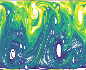





1. Introduction
This paper considers two-dimensional (2-D), constant-volume-flux channel flow for Reynolds numbers  $Re \leq 72\,000 \approx 12.5Re_c$, where the one-dimensional plane Poiseuille base flow famously becomes linearly unstable at $Re_c:=5772.22$ (Orszag Reference Orszag1971). The motivation for considering this simplified flow was a wish to re-examine the statistical stability of turbulent flows using an approach incorporating more statistical information than that originally proposed in Malkus's seminal work (Malkus Reference Malkus1956). Malkus suggested that turbulent mean flows should be statistically marginally stable and proposed that an Orr–Sommerfeld eigenvalue problem constructed around the turbulent mean could be used to assess this. However, a simple parametrisation of some turbulent mean profiles was later found to be quite stable (Reynolds & Tiederman Reference Reynolds and Tiederman1967), which caused the general idea to be largely ignored. The success of recent work assuming the mean flow profile to then predict the structure of the accompanying fluctuation fields – known latterly as ‘resolvent analysis’ (McKeon Reference McKeon2017) – has highlighted the significance of finding a predictive theory for the mean flow if at all possible. Given this, a 2-D channel flow was chosen to revisit the theory because it offers a computationally-accessible environment which contains (2-D) turbulence. Preliminary computations of the turbulent mean profile as a function of $Re$ revealed some unexpected non-uniqueness, which is the subject of this paper.
Channel flow is a canonical shear flow (along with plane Couette and pipe flows) which has been well studied, as the base flow experiences a subcritical Hopf bifurcation at  $Re=Re_c$ where a family of travelling waves is borne (e.g. Chen & Joseph Reference Chen and Joseph1973; Zahn et al. Reference Zahn, Toomre, Spiegel and Gough1974; Orszag & Kells Reference Orszag and Kells1980; Pugh & Saffman Reference Pugh and Saffman1988; Mellibovsky & Meseguer Reference Mellibovsky and Meseguer2015). These (lower branch) waves extend down to $Re \approx 2900$ (Herbert Reference Herbert1979) before turning back (the upper branch) to higher $Re$. More importantly, however, the presence of the bifurcation leads to ever more complicated 2-D dynamics as $Re$ increases, in contrast to 2-D plane Couette (Falkovich & Vladimirova Reference Falkovich and Vladimirova2018) and axisymmetric pipe flows (Willis & Kerswell Reference Willis and Kerswell2009). One of the few studies by direct numerical simulation (DNS) of volume-flux-driven 2-D channel flows was conducted by Jiménez (Reference Jiménez1990) who showed that the (upper branch) travelling wave solutions undergo further bifurcations into a limit cycle at $Re=5400$ and into a two-frequency torus at $Re=9200$. Owing to resolution limitations, only Reynolds numbers $Re \leq 10^4 \approx 1.73Re_c$ were studied in these simulations with full ‘turbulence’ suspected beyond $Re=10^5 \approx 17.3 Re_c$. Umeki (Reference Umeki1994) investigated the wall-layer of the mean turbulent velocity profile of 2-D channels, however, the time scale over which the statistical data was collected turned out to be much shorter than the time scale over which the flow was evolving. More recently, a DNS study of thin fluid layers by Falkovich & Vladimirova (Reference Falkovich and Vladimirova2018) (hereafter FV18) explored a 2-D channel flow driven by a constant pressure gradient up to very high Reynolds numbers ( $Re=3.2\times 10^5 \approx 55.4Re_c$). A thorough description of the flow evolution in short channels with increasing $Re$ was given along with the relationship between the driving pressure gradient and resultant mass flux. Most notably, they found that the turbulent mean flow at higher $Re$ was remarkably similar to that of the travelling wave found at lower $Re$.
$Re$.
The expectation for a 2-D flow where the boundaries and forcing (either pressure gradient or imposed mass-flux) are symmetric about a midline is that the ensuing mean flow response should also be symmetric and unique, at least at sufficiently high  $Re$. Certainly, FV18 does not mention finding any asymmetric mean flows – quantified in the following as the normalised difference between the two average wall shear stresses – in their study, although at least one of their plots hints at such (see § 3.1). Here, we report such states coexisting with the expected symmetric state for mass-flux-driven 2-D channel flows over the range $Re \in [21\,000,42\,000]$ (the asymmetric state was also found in a constant pressure-driven 2-D channel). This ‘asymmetric’ range in $Re$ can be subdivided into regions of low asymmetry, high asymmetry and a transition region in between where the asymmetry intermittently switches between the two levels. The asymmetric states are shown to persist over 48 000 time units ( $=32\,000\,h/U$), which indicates that even if they are only metastable, they are metastable over such a long time scale for this to be significant (e.g. Jiménez (Reference Jiménez1990) gathered statistics over periods up to 6000 time units while Umeki (Reference Umeki1994) used a window of only 32 time units). Our results then add 2-D channel flow to the list of other turbulent flows where multistability has also been observed such as Rayleigh–Bénard convection (Xi & Xia Reference Xi and Xia2008), von Kármán flow (Ravelet et al. Reference Ravelet, Marié, Chiffaudel and Daviaud2004; Faranda et al. Reference Faranda, Sato, Saint-Michel, Wiertel, Padilla, Dubrulle and Daviaud2017), Taylor–Couette flow (Huisman et al. Reference Huisman, van der Veen, Sun and Lohse2014), rotating spherical Couette flow (Zimmerman, Triana & Lathrop Reference Zimmerman, Triana and Lathrop2011), spanwise-rotating plane Couette flow (Xia et al. Reference Xia, Shi, Cai, Wan and Chen2018), 2-D forced shear flow (Dallas, Seshasayanan & Fauve Reference Dallas, Seshasayanan and Fauve2020), flow in a T-mixer (Schikarski et al. Reference Schikarski, Trzenschiok, Peukert and Avila2019) and the flow past a pendular disk in a wind tunnel (Gayout, Bourgoin & Plihon Reference Gayout, Bourgoin and Plihon2021).
Finally, by exploring the basin boundary between the attracting symmetric and asymmetric turbulent states, a travelling wave solution is found as an unstable ‘edge’ state sitting between the two turbulent attractors in phase space. This travelling wave solution originates from the primary bifurcation in the computational domain near  $Re_c$. The end product of this work is that two stable turbulent states parametrised by $Re$ are obtained as data for an investigation of theoretical approaches to assess statistical stability.
2. Set-up
We consider a 2-D channel of height  $2h$ along which a pressure gradient $G$ is applied to drive a constant volume flux $2hU$. Using $h$ and $\frac {3}{2}U$ (see directly below (2.2a,b) for why) to non-dimensionalise the system, the computational domain is $(x,y) \in [0,8) \times [-1,1]$ with periodic boundary conditions in $x$ and no-slip walls at $y=\pm 1$, as was studied by Falkovich & Vladimirova (Reference Falkovich and Vladimirova2018), and time is measured in units of $=2h/3U$. We impose constant volume flux by insisting that
 \begin{equation} \int_{{-}1}^1\boldsymbol{u}(x,y,t) \cdot \hat{\boldsymbol{x}}\,{\textrm{d}y}=\tfrac{4}{3}. \end{equation}
Two Reynolds numbers are defined as
 \begin{equation} Re:= \frac{3U h}{2 \nu} \quad \textrm{and} \quad Re_P:= \frac{G h^3}{2 \nu^2},\end{equation}
where  $\nu$ is the kinematic viscosity. Here, $Re$ is the control parameter based upon the constant mass flux and $Re_P$ is an output which measures the pressure gradient needed to maintain this mass flux. These are equal when the flow is laminar because the centreline speed $U^c:=Gh^2/2\nu =\frac {3}{2}U$ for the laminar parabolic flow profile. Using a streamfunction $\psi$, so that $(u,v)=(\psi _y,-\psi _x)$ reduces the system down to a scalar vorticity ( $\omega$) equation,
 \begin{equation} \omega_t + \psi_y \omega_x - \psi_x \omega_y = \frac{1}{Re} \nabla^2 \omega, \quad \omega={-} \nabla^2 \psi \end{equation}
with boundary conditions
 \begin{equation} \psi\left({-}1\right)=0, \quad \psi\left(1\right)=\tfrac{4}{3}, \quad \psi_y\left({-}1\right)=0, \quad \psi_y\left(1\right)=0. \end{equation}
For turbulent flows,  $Re_P>Re$, because more pressure is required to drive a turbulent flow than a laminar flow with the same volume flux. FV18 found that $Re_P\simeq Re^{{3}/{2}}$ for the solutions they computed. In this paper, we describe a new stable branch of solutions asymmetric with respect to the midplane of the channel which has a different $Re_P$– $Re$ relationship.
As an output of the flow,  $Re_P$ is found by bulk-averaging the $x$-momentum equation,
 \begin{equation} Re_P(t)={-}\frac{Re}{4}\left[\left.\frac{\partial \bar{u}^{x}}{\partial y}\right|_{y=1}- \left.\frac{\partial \bar{u}^{x}}{\partial y}\right|_{y={-}1}\right] \end{equation}
(where  $\bar {u}^{x}$ indicates a streamwise average of $u$) as the time derivative of the bulk $x$-momentum is zero by constant mass flux. Finally, to quantify the asymmetric behaviour of the newly found states, we define the asymmetry coefficient $A\in [-\frac {1}{2},\frac {1}{2}]$ as
 \begin{equation} {A}(t)\ {:=}\ \frac{1}{2}\frac{\left| \dfrac{\textrm{d}\bar{u}^{x}}{\textrm{d}y}|_{y=1}\right| - \left|\dfrac{\textrm{d}\bar{u}^{x}}{\textrm{d}y}|_{y={-}1} \right| }{\left| \dfrac{ \textrm{d}\bar{u}^{x} }{\textrm{d}y}|_{y=1} \right|+ \left| \dfrac{\textrm{d}\bar{u}^{x} }{\textrm{d}y}|_{y={-}1} \right|}. \end{equation}
 A definition of (statistically) symmetric flows as those with  $\bar {A}^{^t} \approx 0$ to within $\pm 0.01$ proved a simple and robust way to distinguish between symmetric and asymmetric states for the time period chosen for averaging. The kinetic energy averaged over the domain
 \begin{equation} {E}(t)\ {:=}\ \frac{1}{16}\int_{{-}1}^1 \int_{0}^8 \frac{1}{2}(u^2+v^2)\,{\textrm{d}x}\,{\textrm{d}y} \end{equation}
was also considered with an accompanying variable  $E_k(t)$ used to represent the contribution to $E$ from the $(4k/{\rm \pi} )$th streamwise Fourier mode (the smallest wavenumber for the computational domain is ${\rm \pi} /4$).
2.1. Numerical procedure
Equation (2.3) was solved numerically together with the boundary conditions (2.4a–d) using the open-source partial differential equation solver Dedalus (Burns et al. Reference Burns, Vasil, Oishi, Lecoanet and Brown2020). The solver uses a Fourier–Chebyshev decomposition in the  $x$ and $y$ directions respectively with resolutions $(N_x,N_y)$ given in table 1. For time integration, an implicit-explicit Runge–Kutta RK443 time stepper with an adaptive time step was chosen. The Courant number was set to a low value of $0.6$ with the fractional change threshold for changing the time step set to $0.1$ to increase simulation speed.
Table 1. Numerical data generated. S1 is the region where only symmetric states were detected; SA1, SA2, SA3 are the regions with degeneracy of symmetric and asymmetric states; EDGE denotes the edge state at  $Re=36\,300$; S2 is the region where symmetry is obtained but only over very long times. For further information, refer to the text in § 3.2. Here, $(N_x,N_y)$ is the gridpoint resolution used in the simulation; $Re_P$ is the pressure-gradient-based Reynolds number (see (2.2a,b)); $\varDelta \%$ is the percentage difference in $Re_P$ values between our results and the corresponding states from FV18 if such states are available, otherwise, an estimated value of $Re_P$ is taken by interpolating between two FV18 data points. $\bar {A}^{^t}$ is the time-averaged asymmetry parameter (see (2.9a,b)); $\sigma _A$ is the standard deviation of asymmetry fluctuations in time, also used as the error bars in figure 2; $Re_{\tau }$ is the friction Reynolds number (see (2.11)).

The asymmetric states were initiated at  $Re=36\,300$ by perturbing the laminar profile as
 \begin{equation} \psi_0=\psi_{lam}+\psi_{pert}=\left(y-\frac{1}{3}y^3-\frac{2}{3}\right)-\frac{4}{3{\rm \pi}^2}\sin^2{{\rm \pi} y} \sin{\frac{\rm \pi}{4}x}, \end{equation}
which satisfies the boundary conditions and has an antisymmetric (in  $y$) streamwise velocity perturbation (subsequently, other asymmetric perturbations were also found which lead to the asymmetric turbulent state). The newly-found asymmetric branch was then explored by using a snapshot of this new state as the initial condition in DNS at higher and lower $Re$.
$Re$.
Unless otherwise stated, the time averaging procedure was as follows. The data for the asymmetric states were collected in the time window  $t\in [0,48\,000]$ and averaging performed over $t\in [t_1 = 9000,\ t_2=48\,000]$ to avoid transient behaviour, i.e.
 \begin{equation} {\bar{A}}^{t} := \frac{1}{t_2-t_1} \int_{t_1}^{t_2} {A}(t)\,\textrm{d} t, \quad {\overline{Re_P}}^{t} := \frac{1}{t_2-t_1} \int_{t_1}^{t_2} {Re_P}(t)\,\textrm{d} t. \end{equation}
 Symmetric states exhibited much shorter transient periods and were oscillating on much shorter time scales so data were collected in the time window  $t\in [0,21\,000]$ and the averaging was conducted for $t\in [t_1=3000,\ t_2=21\,000]$ instead. This applies to all runs of symmetric states except for $Re=60\,000$ and $72\,000$, where large fluctuations were observed over a long period and the more extensive averaging procedure of the asymmetric states was used. The edge tracking technique (Itano & Toh Reference Itano and Toh2001; Skufca, Yorke & Eckhardt Reference Skufca, Yorke and Eckhardt2006; Schneider, Eckhardt & Yorke Reference Schneider, Eckhardt and Yorke2007) was used to find an unstable (saddle) state on the basin boundary separating the asymmetric and symmetric turbulent attractors.
2.2. Near-wall rescaling
Owing to the possible asymmetric nature of the flow, viscous effects near the two channel walls may differ on average. Hence, two sets of viscous units were used to rescale the velocity profiles and other quantities near the two channel walls (see § 3.2 for relevant plots).
A friction velocity near the top (bottom) channel wall was defined in the usual way as
 \begin{equation} u_{\tau}^{{\pm}} = \sqrt{\left|\frac{1}{Re} \frac{ \partial \bar{u}^{x,t}}{\partial y}\right|}_{y=\pm1}. \end{equation}
Here,  $\bar {u}^{x,t}$ indicates the streamwise and time average of $u$. We plot the rescaled quantities against the rescaled distance from the top (bottom) wall, $y^+=Re(1-y)u_{\tau }^+$ ( $y^-=Re(1+y)u_{\tau }^-$), and evaluate the (averaged) friction Reynolds number (see table 1) as
 \begin{equation} Re_{\tau}= \tfrac{1}{2}(u_{\tau}^+{+}u_{\tau}^-)Re. \end{equation}
3. Results
Perturbing the laminar flow at  $Re=36\,300$, as defined by (2.8), results in an asymmetric state. The asymmetry is clearly visible from the mean velocity profile $\bar {u}^{x,t}$ and root-mean-square velocity profiles, $u_{RMS} := \overline {u^2}^{x,t} - (\bar {u}^{x,t})^2$, $v_{RMS} := \overline {v^2}^{x,t} - (\bar {v}^{x,t})^2$, plotted in figure 1. The mean profiles of the asymmetric and symmetric states are quite different (see solid lines in figure 1a): the asymmetric profile has clearly visible asymmetry with respect to the centreline of the channel. It also has larger maximum velocity at the nose ( $=1.005$) of the profile compared with the symmetric profile ( $=0.902$) at the expense of slower velocity near the top channel wall (recall both profiles have the same volume flux and the centreline speed for the Poiseuille base flow is $1$). Finally, while the wall layer near the bottom wall is similar in both of the profiles, significantly less shear is observed near the top wall of the asymmetric profile. The difference in the shear at the top and bottom channel walls motivates the definition of the asymmetry (2.6). Similar observations can be made when considering the RMS velocities of both of the states: while the overall magnitude of the RMS profiles is of comparable size in both states, the RMS profiles of the asymmetric state are noticeably suppressed near the top wall.

Figure 1. Velocity profiles of  $Re=36\,300$ symmetric (light blue), asymmetric (light pink) and laminar (black) states. (a) Streamwise mean velocity profile $\bar {u}^{x,t}$ (solid line) and $u_{RMS}$ (dashed line); (b) streamwise $u_{RMS}$ (dashed line) and wall-normal $v_{RMS}$ (dotted line). Time averaging is over ${\rm \Delta} t =5000$ time units.
In this section, we first investigate how the asymmetry changes with Reynolds number and outline where these states coexist with the symmetric state. Then, we compare the turbulent properties of the symmetric and asymmetric states. Finally, we explore the unstable manifold between symmetric and asymmetric states at  $Re=36\,300$, where the difference between the two stable states is the most significant.
3.1. Degeneracy of turbulent states
The  $Re$ range over which the pair of asymmetric turbulent states coexists with the symmetric state described in FV18 (at least for $48\,000$ time units) is designated as region SA. In contrast, region S1 indicates where only the symmetric state is stable and region S2 indicates where the state also looks to be symmetric when averaged over an extremely long time. Investigation of the asymmetry parameter $A(t)$ for the states in this region revealed the existence of two discrete asymmetry levels: higher and lower. This feature suggests further dividing the region SA into three sub-regions: SA1, where the asymmetry is low; SA2, where the asymmetry is repeatedly jumping between the lower and higher levels; and SA3, where the asymmetry is high. Typical time signals of the asymmetry parameter in these three regions are shown in figure 2. Further significance of the three subregions is revealed by investigating the relationship between the pressure gradient and volume flux of the asymmetric states and comparing the resulting asymmetric solution branch to the solution branch of the symmetric state. Figure 3(a) shows the symmetric and asymmetric states in terms of $Re$ and their $Re_P$. While for laminar flows, $Re_P=Re$ (shown as black dashed line in the diagram), the symmetric turbulent state obeys a $Re_P\propto Re^{{3}/{2}}$ relationship, as was first shown by FV18. Figure 3(b) shows the time-averaged asymmetry parameter $\bar {A}^{^t}$ at different Reynolds numbers together with the error bars indicating the standard deviation of the temporal fluctuations.

Figure 2. Time evolution of the asymmetry parameter  $A(t)$. (a) Asymmetric states in: region SA1 – $Re=21\,000$ (dark green), $Re=22\,350$ (light green); region SA2 – $Re=24\,000$ (yellow), $Re=26\,250$ (orange), $Re=30\,000$ (brown); region SA3 – $Re=33\,750$ (red), $Re=36\,300$ A (light pink), $Re=46\,875$ (dark pink). (b) Comparison of $A(t)$ of a symmetric state, $Re=36\,300$ S (light blue; see the inset on the right for zoomed-in fluctuations) with $A(t)$ of the unstable (initially) symmetric state at $Re=43\,000$ (dark purple) resulting in an asymmetric state. Black solid line in the left inset also shows the instability of the asymmetric state at $Re=20\,000$. (c) Region S2 states at $Re=60\,000$ (light grey) and $Re=72\,000$ (dark grey) together with the representative states of regions SA1 ( $Re=22\,350$, light green) and SA3 ( $Re=33\,750$, red).

Figure 3. Degeneracy of turbulent states in 2-D channels: blue and grey squares, symmetric states; coloured circles, asymmetric states (colours as in figure 2); black open circle, edge state at  $Re=36\,300$. (a) The $Re_P$ as a function of $Re$. Here, $Re_P=Re$ is marked by the black dashed line and results from FV18 are marked by black crosses. (b) The ${\bar {A}^{^t}}$ as a function of $Re$. The error bars signify $\sigma _A$ (see table 1). Black dashed lines correspond to asymmetry averaging over the highest and the lowest $10\,\%$ of values.
In region SA1, where  $Re \in [21\,000,24\,000)$, the asymmetric states have a relatively steady asymmetry signal of $\bar {A}^{^t}\approx 0.05$ with only very small fluctuations around this value, as shown in figure 2 and the error bars in in figure 3(b). In contrast, figure 2(b, inset) shows that $A$ fluctuates around 0 with an amplitude $\approx 0.001$ for the symmetric state. While the asymmetric states possess significant asymmetry, their corresponding $Re_P$ value is very close to the symmetric flow value being within $1\,\%$ of each other (see figure 3a). As a consequence, in this region, the asymmetric states are hard to detect. At $Re=20\,000$, only monotonic decay of asymmetry was found: see figure 2(b).
Region SA2, where  $Re \in [24\,000,33\,750)$, is the transitional region because the asymmetry signal of the asymmetric states repeatedly jumps between the lower and higher asymmetry levels. The ratio of the time spent at the higher level to the time spent at the lower level increases with Reynolds number $Re$. When time averaging, this results in large asymmetry fluctuations around an increasing average asymmetry value, as is indicated in figure 3 (bottom). Conditional averaging instead, by only using the highest $10\,\%$ and the lowest $10\,\%$ of the asymmetry signal, indicates how the higher and lower asymmetry branches extend across this region (see the dashed lines in 3b). In terms of $Re_P$, region SA2 in figure 3(a) shows the asymmetric solution branch detaching from the symmetric solution branch with a gradually growing gap in the $Re_P$ value.
In region SA3, where  $Re \in [33\,750,46\,875+]$ (the region extends past $46\,875$ but not as far as $60\,000$), the asymmetry signal of the asymmetric states stays at a higher level – $\bar {A}^{^t}\approx 0.28$ – with the level of chaotic fluctuations indicating a more turbulent behaviour. The asymmetric states follow the new solution branch with differences between the $Re_P$ values of symmetric and asymmetric states being as high as $22\,\%$ for $Re = 36\,000$.
In regions S1, SA1, SA2 and SA3 up to  $Re=42\,000$, the symmetric states are in good qualitative (travelling wave structure) and quantitative (see table 1 for $\varDelta \%$ values) agreement with FV18. The asymmetry fluctuations of these states are at most $0.001$, as shown in figure 2(b). However, the symmetric branch cannot be tracked beyond $Re=42\,000$: using the symmetric state at $Re=42\,000$ in a simulation at $Re=43\,000$ results in an asymmetric SA3 region state (see figure 2b).
In region S2, which starts somewhere between  $Re=46\,875$ and $60\,000$, the asymmetric state also changes its qualitative behaviour: the asymmetry parameter $A$ experiences large fluctuations in time and changes sign on a time scale which decreases as the Reynolds number increases (see figure 2c). These asymmetry fluctuations should plausibly cancel out to give a new type of symmetric state when averaged over an extremely long time window.
These states showing non-trivial asymmetric behaviour are the only states we found in S2 region, which raises the question whether the asymmetric behaviour was also observed by FV18, as figure 4 in their paper might suggest. At  $Re=1.5\times 10^5$, the time-averaged vorticity appears to have a significantly larger absolute value at the negative than at the positive vortex. Additionally, the proximity of a FV18 data-point to our asymmetric state at $Re=46\,875$ (which is beyond the symmetric state instability point at $Re=43\,000$) in figure 3 also suggests asymmetry.
3.2. Asymmetric path to turbulence
The symmetric state first observed by FV18 was considered to have reached turbulence at approximately  $Re=30\,000$, when small vortices created at the channel wall were observed to be swept into the main vortex. The asymmetric states, however, show higher turbulence levels to their symmetric counterparts, with early signs of turbulence appearing at much lower Reynolds numbers, which suggests the asymmetric states undergo a different path to turbulence to their symmetric counterparts. To compare turbulent properties of the symmetric and asymmetric states, the mean velocity $\bar {u}^{x,t}$, Reynolds stress $\overline {uv}^{x,t}$ and production of turbulent kinetic energy $P=\overline {uv}^{x,t}\,\textrm {d}\bar {u}^{x,t}/{\textrm {d}y}$, rescaled with viscous wall units as explained in § 2.2, are shown in figure 4 (all time-averaged over ${\rm \Delta} t = 5000$ time units). Asymmetric states show larger turbulence production and Reynolds stress peaks near the ‘turbulent’ wall than near the ‘quiet’ wall, and, more importantly, than their symmetric counterparts. For all states, the power spectrum $E_k/E$ (see (2.7) for definition), shows evidence of the direct cascade scaling law $k^{-3}$ for 2-D turbulence (Kraichnan Reference Kraichnan1967) (see figure 5).

Figure 4. (a,b) Mean profile  $\bar {u}^{x,t}$; (c,d) Reynolds stress $\overline {uv}^{x,t}$; and (e,f) turbulence production $P$. All quantities are shown in viscous wall units as defined in § 2.2 and $u^*_{\tau }$ corresponds to $u^{+}_{\tau }$ ( $u^{-}_{\tau }$) used for rescaling near the top (bottom) channel wall. (a,c,e) Reynolds number $Re=22\,350$ (light green); (b,d,f) $Re=36\,300$ (light pink) and $Re=43\,000$ (purple). Solid lines correspond to symmetric states (note, for $Re=43\,000$, the symmetric state at $Re=42\,000$ is shown instead), dashed lines correspond to asymmetric states near the ‘turbulent’ wall and dotted lines correspond to asymmetric states near the ‘quiet’ wall.

Figure 5. Velocity power spectrum  $E_k/E$, see (2.7). (a) Reynolds number $Re=22\,350$ (light green); (b) $Re=36\,300$ (light pink) and $Re=43\,000$ (purple). Solid lines correspond to symmetric states (note, for $Re=43\,000$, the symmetric state at $Re=42\,000$ is shown instead) and dashed lines correspond to asymmetric states. Dashed black line shows the direct cascade scaling of $k^{-3}$ for 2-D turbulence.
The difference in turbulent activity between the symmetric and asymmetric states manifests itself in the vorticity field. Figure 6 shows sample instantaneous vorticity fields (See supplementary movies available at https://doi.org/10.1017/jfm.2021.336 for full videos). Like all symmetric states in regions S1 and SA, the symmetric state at  $Re=36\,300$ (figure 6a) consists of an almost steady travelling wave with two vortices at each of the channel walls: the vortices are all the same magnitude and experience only minor fluctuations. The asymmetric state at $Re=22\,350$ in region SA1 (figure 6b) has one of the two vortices near the bottom channel wall starting to break up, displaying larger amplitude chaotic fluctuations which causes the asymmetry. By region SA3, the chaotic behaviour has spread into both the bottom wall vortices resulting in a higher level of asymmetry (figure 6c). Presumably, a longer (computational) channel harbouring more vortices would give rise to a corresponding larger number of asymmetry levels. The asymmetry fluctuations of the asymmetric state are also larger than those of the symmetric state at $Re=36\,300$ (see figure 2a). Hence, more irregular, ‘turbulent’ behaviour is observed at much lower Reynolds numbers for the asymmetric than symmetric states.

Figure 6. Snapshots of: (a,b) the vorticity field  $\omega (t)$; (c,d) time-averaged vorticity field $\bar {\omega }^t$ in the travelling wave frame; and (e,f) the fluctuation field $\omega (t)-\bar {\omega }^t$ for (a) the symmetric state at $Re=36\,300$, (b) the asymmetric state at $Re=22\,350$ (‘lower-level’ asymmetry), (c) $Re=36\,300$ (‘higher level’ asymmetry), (d) numerical approximation to the edge state at $Re=36\,300$, (e) $Re=72\,000$ (positive asymmetry region) and (f) $Re=72\,000$ (negative asymmetry region). For $Re=72\,000$, time averaging is done in a window of 150 time units to preserve the asymmetric behaviour. There are 100 contour levels between $-4$ (dark blue) and $4$ (yellow). In the $\omega (t)-\bar {\omega }^t$ diagram of (d), green contours correspond to the value $0.016$, showing very small but non zero vorticity fluctuations. (a) Reynolds number $Re=36\,300$ S; (b) $Re=22\,350$ A; (c) $Re=36\,300$ A; (d) $Re=36\,300$ Edge; (e) $Re=72\,000,\ t=33\,000,\ A(t)>0$; and (f) $Re=72\,000,\ t=45\,000,\ A(t)<0$.
Another important feature of the flow is the jet separating the counter-rotating vortices near the top and bottom walls. FV18 discuss this feature in deriving a scaling prediction for the flux given the pressure gradient. This jet is located at equal distances from both of the walls in the symmetric case, while it separates from the quiet wall and moves towards the turbulent wall in the asymmetric case. This creates an extra viscous barrier which fluctuations created near the turbulent wall need to cross to reach the quiet half of the channel. This helps explain how turbulent fluctuations can stay localised at one wall in the asymmetric states. If  $Re$ is sufficiently increased, vorticity fluctuations become large enough to overcome the jet barrier and all the vortices become contaminated with chaotic fluctuations restoring symmetry on average. Figures 6(e) and 6(f) show vorticity snapshots for the $Re=72\,000$ state where symmetry is restored on average. Interestingly, the main travelling wave structure persists despite the highly turbulent behaviour near both of the channel walls, as also noticed by FV18. Analysing the vorticity snapshots in the regions where asymmetry is either positive or negative, it is seen that the separating jet becomes less rigid and starts fluctuating towards one of the two channel walls. In this manner, the viscous barrier, which existed in asymmetric states at lower Reynolds numbers, can be broken allowing the turbulent vortices to move freely between the two halves of the channel without dissipating.
3.3. Unstable (saddle) state
In the  $Re$ range where the asymmetric and symmetric states are stable, it is natural to look for an unstable or ‘saddle’ state embedded in the manifold or ‘edge’ separating the basins of attraction of the two attractors in phase space. To this end, an edge tracking procedure was performed at $Re=36\,300$ (Itano & Toh Reference Itano and Toh2001; Skufca et al. Reference Skufca, Yorke and Eckhardt2006; Schneider et al. Reference Schneider, Eckhardt and Yorke2007) over $10\,000$ time units in total, with the last $5000$ units revealing a travelling-wave solution. This travelling wave only has non-zero energy $E_k$ at the second-lowest wavenumber and its higher harmonics indicate that it originates in a primary travelling wave bifurcation when $Re\gtrsim Re_c$ (the bifurcation only occurs at $Re_c=5772$ for channel lengths which allow the critical wavenumber $1.02056$ Orszag Reference Orszag1971). Figure 7(b) shows $E(t)$ for selected edge tracking results, which reveal the constant energy level of the travelling wave edge state. The vorticity field of the numerical approximation to the edge state is shown in figure 6(d), which reveals very small but non-zero vorticity fluctuations. States started ‘just above’ the edge separate from the edge with rapid exponential growth towards the symmetric state, while states started ‘just below’ the edge separate from the edge with the same exponential growth, visit the (unstable) laminar state and then converge to the asymmetric state. A simple phase-space portrait is shown in figure 7(a) to rationalise the likely situation (note that the states shown are all turbulent states except for the edge and laminar states). Finally, in terms of $Re_P$ values, the edge state is in between the asymmetric and laminar states, as is shown in figure 3(b).

Figure 7. Edge tracking results. (a) Schematic representation of the energy, which presents an asymmetry projection of phase-space showing relative positions of asymmetric  $A^-,A^+$ and symmetric $S$ stable states together with unstable edge $E$ and laminar $L$ states. Red curves indicate edge tracking trajectories for states ‘just above’ the edge ( $\lambda ^+$) leading to the $S$ state, and ‘just below’ the edge ( $\lambda ^-$) leading to the asymmetric $A^+$ state. Shaded regions represent the basins of attraction of $S$ (blue), $A^+$ (red) and $A^-$ (brown) states. (b) Kinetic energy, $E(t)$, evolution for selected edge-tracking results. Average energy levels of the symmetric (light blue), asymmetric (light pink), edge (grey) and laminar (black) states are marked by dashed lines.
4. Conclusions
In this paper, a volume-flux-driven flow through a streamwise-periodic two-dimensional channel with a length-to-height ratio of 4 was studied by direct numerical simulations. A degeneracy of turbulent states was discovered for  $Re\in [21\,000,42\,000]$. In this region, symmetric states resembling travelling waves with a wavelength of half the channel length were found to coexist with asymmetric states which maintain the same travelling wave structure but show heightened turbulent behaviour near one of the channel walls. Both of these states were found to be stable for at least 48 000 time units (or $32\,000\,h/U$).
At lower Reynolds numbers,  $Re \in [21\,000,24\,000)$, the asymmetric states are largely indistinguishable from their symmetric counterparts in terms of their $Re_P$ value, while at higher Reynolds numbers, the difference in $Re_P$ can reach $22\,\%$. There, asymmetric states form a separate branch to the original solution branch characterised by the $Re_P \propto Re^{{3}/{2}}$ law. In the chosen geometry, the asymmetric states follow an interesting path to turbulence. Chaotic behaviour originates first at one of the travelling vortices near the turbulent channel wall. Then, as the Reynolds number is increased, turbulence spreads to both of the travelling vortices near the turbulent channel wall before, at some $Re$, the vortices at the other wall become similarly chaotic. In a longer channel fitting $n$ vortices along the wall, there should be $n$ discrete asymmetry levels observed with increasing Reynolds number. As the Reynolds number is increased even further, the symmetric states are found to become unstable by $Re=43\,000$, which leaves the asymmetric states as the only states observed up to approximately $Re=60\,000$, when chaotic asymmetry fluctuations and sign changes indicate that the overall symmetry of the states can be recovered when averaged over extremely long times ( $\gg 10^5 h/U$).
While our study is limited to one specific domain and a relatively narrow window of  $Re$, owing to the computational cost of simulating for long times, it offers new insight into the complexity of turbulent 2-D flows. The first signs of turbulent behaviour in 2-D channels were found by Jiménez (Reference Jiménez1990), but it was not until 2018 that the truly turbulent regime was reached by FV18, who showed the robustness of the travelling wave structure at high Reynolds numbers. Even at $Re=3.2 \times 10^5$, the signature of the initial bifurcation is still clear. We have extended the story by discovering at least a metastability of states if not the degeneracy of turbulent attractors at relatively low Reynolds numbers which possess different symmetry properties yet still exhibit the same robust travelling wave structure. Moreover, we have also shown that the saddle state sitting on the basin boundary of the two attractors corresponds to a simple travelling wave which can trace its origin to an initial bifurcation off the basic unidirectional steady state. In terms of our initial motivations, which was to generate turbulent flows in a numerically-accessible shear flow as data for revisiting the idea of marginal statistical stability (Malkus Reference Malkus1956), this work has been more fruitful than envisaged. We have twice the amount of data we expected for stable turbulent states (the asymmetric as well as the symmetric states). This then provides a good basis for testing different approaches for assessing the statistical stability, which we hope to report on in the near future.
Supplementary movies
Supplementary movies are available at https://doi.org/10.1017/jfm.2021.336.
Acknowledgements
The authors are particularly grateful to one of the reviewers for a thoughtful report on the original manuscript.
Funding
V.K.M. acknowledges financial support from EPSRC through a studentship.
Declaration of interests
The authors report no conflict of interest.


 Open access

