


1. Introduction
In fluid dynamics, dispersion is typically used to denote the transport of a species from high to low concentrations due to non-uniform flow conditions. This is in contrast to diffusion, which denotes the similar transport of a species from high to low concentrations but due to Brownian motion. Since relatively few flow systems actually transport flow in a plug-like way, dispersion is a nearly ubiquitous transport mechanism in systems including microfluidic devices, filtration systems, chemical reactor systems, medical devices, lab-on-a-chip systems and many others. A classical and simple example of dispersion is that which has come to be known as Taylor dispersion, which was first studied by Taylor (Reference Taylor1953) and later generalized by Aris (Reference Aris1956). Taylor dispersion describes the enhanced diffusivity that a diffusing species experiences in the presence of a shear flow, such as the diffusion of a solute concentration field in a pipe or channel flow. In both of these cases, the advection–diffusion equation governing the solute transport can be averaged over the cross-section to yield a one-dimensional (1-D) model for the depth-averaged concentration, which experiences an enhanced effective diffusivity that is a function of the Péclet number governing the transport. A simple physical understanding of this Taylor dispersion can be achieved by supposing we have a step initial condition in the concentration  $c$ of some solute species. For example, suppose we have a Poiseuille flow in a pipe, and we suddenly add solute to the system such that $c(x<0)=c_1$ and $c(x>=0)=c_2$, where $-\infty < x<\infty$ is the axial coordinate of our infinite pipe. Then, in the limit of no background flow, the interface between the two solute concentrations will smear out by diffusion in a purely 1-D process. However, as the relative importance of fluid advection to solute diffusion (i.e. the Péclet number) increases, shear flows in the system distort the interface between the two solute concentrations as they diffuse, introducing cross-stream diffusion and enhancing the rate of axial diffusion of the cross-sectionally averaged concentration. For more rigorous background into the Taylor dispersion phenomenon, see (i) Barton (Reference Barton1983), who extended the methods and results of Aris (Reference Aris1956) to consider all times rather than just the asymptotic behaviour, (ii) Frankel & Brenner (Reference Frankel and Brenner1989), who developed a generalized Taylor dispersion theory to greatly extend the ideas of Taylor and Aris to whole classes of other problems such as porous medium flows or even sedimenting particles and (iii) Brenner & Edwards (Reference Brenner and Edwards1993), who provide a comprehensive overview of the theory of macrotransport processes.
Many other studies and applications have built upon the theoretical work on Taylor dispersion by Taylor and Aris. Here, we just briefly mention a few examples. Stone & Brenner (Reference Stone and Brenner1999) extended the theories of Taylor dispersion to consider laminar flows with velocity variations in the streamwise direction. Aminian et al. (Reference Aminian, Bernardi, Camassa, Harris and McLaughlin2016) studied the role of the channel boundary shape and aspect ratio on the dispersion as a means to control the delivery of chemicals in microfluidics. Salmon & Doumenc (Reference Salmon and Doumenc2020) studied the solute dispersion induced by buoyancy-driven flow and developed analytical methods analogous to Taylor dispersion. Chu et al. (Reference Chu, Garoff, Przybycien, Tilton and Khair2019) added the ideas of oscillatory pressure-driven flow in a parallel-plate channel flow as well as patterned slip walls and investigated the role of both of these effects on the dispersion process. Finally, Chu et al. (Reference Chu, Garoff, Tilton and Khair2021) coupled the Taylor dispersion in a pipe flow to the transport of a second species consisting of particles or bacteria via diffusiophoresis, which was also explored by Migacz & Ault (Reference Migacz and Ault2022). This list is by no means exhaustive, but one unifying theme that is common to many of the studies related to dispersion is the role of imposed pressure gradients or moving boundaries to drive the shear flows that cause the dispersion. Typically, the transport of the solute is passive in the sense that it is not expected to couple to and alter the background fluid dynamics. However, there are many scenarios where the transport of solute is fully coupled to the fluid dynamics, which is the focus of this paper. In particular, we consider the case where there is no background pressure-driven flow and no moving boundaries, but where the solute interacts with the boundaries of the system to drive fluid flow via diffusioosmosis, which is the spontaneous motion of fluid near a surface in the presence of a solute concentration gradient.
The physical origin of diffusioosmosis was discovered by Derjaguin, Dukhin & Korotkova (Reference Derjaguin, Dukhin and Korotkova1961), where Derjaguin and his coworkers showed experimentally that a local solute concentration gradient near a boundary could induce a slip-flow boundary condition over the surface. Since then, significant theoretical progress has been made towards understanding and modelling this effect, and in the context of dispersion, a variety of studies have demonstrated the potential for diffusioosmosis to alter the transport of suspended species in confined geometries (Keh & Ma Reference Keh and Ma2005; Kar et al. Reference Kar, Chiang, Ortiz Rivera, Sen and Velegol2015; Shin et al. Reference Shin, Um, Sabass, Ault, Rahimi, Warren and Stone2016, Reference Shin, Ault, Warren and Stone2017b; Ault, Shin & Stone Reference Ault, Shin and Stone2019; Rasmussen, Pedersen & Marie Reference Rasmussen, Pedersen and Marie2020; Chakra et al. Reference Chakra, Singh, Vladisavljević, Nadal, Cottin-Bizonne, Pirat and Bolognesi2023). Diffusioosmosis is also closely related to the analogous phenomenon of diffusiophoresis. Whereas diffusioosmosis refers to the motion of fluid next to a surface in the presence of a chemical concentration gradient, diffusiophoresis refers to the reciprocal motion of suspended particles in a concentration gradient, which results due to the slip flow at the surface. Both diffusioosmosis and diffusiophoresis can make contributions due to chemi-osmosis/-phoresis that arises from the osmotic pressure gradient over the surface and electro-osmosis/-phoresis that arises in the case of electrolyte solutes with mismatched anion and cation diffusivities (Anderson & Prieve Reference Anderson and Prieve1984). Coupled diffusioosmosis and diffusiophoresis has been the subject of a variety of recent studies, especially concerning the coupled transport of solutes and colloidal particles in confined geometries where convective transport is difficult to achieve, such as in dead-end pores, microgrooved channels and other confined systems (Kar et al. Reference Kar, Chiang, Ortiz Rivera, Sen and Velegol2015; Shin et al. Reference Shin, Ault, Feng, Warren and Stone2017a; Shin, Warren & Stone Reference Shin, Warren and Stone2018; Ha et al. Reference Ha, Seo, Lee and Kim2019; Singh et al. Reference Singh, Vladisavljević, Nadal, Cottin-Bizonne, Pirat and Bolognesi2020; Williams et al. Reference Williams, Lee, Apriceno, Sear and Battaglia2020; Alessio et al. Reference Alessio, Shim, Mintah, Gupta and Stone2021; Shi & Abdel-Fattah Reference Shi and Abdel-Fattah2021; Singh et al. Reference Singh, Chakra, Vladisavljević, Cottin-Bizonne, Pirat and Bolognesi2022a,Reference Singh, Vladisavljevic, Nadal, Cottin-Bizonne, Pirat and Bolognesib; Chakra et al. Reference Chakra, Singh, Vladisavljević, Nadal, Cottin-Bizonne, Pirat and Bolognesi2023).
Such coupled motions have also been the focus of studies in a variety of other natural and engineering settings, such as in underground porous medium flows (Park et al. Reference Park, Lee, Yoon and Shin2021), water filtration systems (Florea et al. Reference Florea, Musa, Huyghe and Wyss2014; Shin et al. Reference Shin, Ault, Warren and Stone2017b; Lee et al. Reference Lee, Kim, Yang, Seo and Kim2018; Bone, Steinrück & Toney Reference Bone, Steinrück and Toney2020), microfluidic devices (Palacci et al. Reference Palacci, Abécassis, Cottin-Bizonne, Ybert and Bocquet2010; Shin et al. Reference Shin, Shardt, Warren and Stone2017c), fabric cleaning systems (Shin et al. Reference Shin, Warren and Stone2018), particle delivery methods (Ault et al. Reference Ault, Warren, Shin and Stone2017; Singh et al. Reference Singh, Vladisavljevic, Nadal, Cottin-Bizonne, Pirat and Bolognesi2022b), energy storage applications (Gupta et al. Reference Gupta, Rajan, Carter and Stone2020a; Gupta, Zuk & Stone Reference Gupta, Zuk and Stone2020c) and many others. Typically, in such studies the role of diffusioosmosis has been a secondary effect, or neglected entirely, although a collection of studies on the motion of solutes and particles in narrow pores has considered both effects (Ault et al. Reference Ault, Warren, Shin and Stone2017; Shin et al. Reference Shin, Ault, Feng, Warren and Stone2017a; Singh et al. Reference Singh, Vladisavljević, Nadal, Cottin-Bizonne, Pirat and Bolognesi2020; Williams et al. Reference Williams, Lee, Apriceno, Sear and Battaglia2020; Alessio et al. Reference Alessio, Shim, Mintah, Gupta and Stone2021, Reference Alessio, Shim, Gupta and Stone2022). In such systems, diffusioosmosis can play an essential role in the transport of the solutes, the fluid and any suspended particles (Shim Reference Shim2022). In the present study, we investigate the dispersion of solute in a channel where the only fluid motion is driven by diffusioosmosis at the channel walls. That is, the diffusion of the initial solute concentration results in a local concentration gradient at the walls that in turn drives a fluid recirculation via diffusioosmosis. The resulting shear flows then in turn alter the transport of the solute concentration by a mechanism analogous to that of Taylor dispersion.
The coupling between particle diffusiophoresis and mixing has been explored in several key works, finding a range of possible interactions. In some, the effects of dispersion/mixing on particle diffusiophoresis are relatively limited. For example, Shah et al. (Reference Shah, Tan, Taylor, Tang, Shi, Mashat, Abdel-Fattah and Squires2022) investigated the temperature dependence of the diffusiophoretic mobility with a novel microfluidic system and found that the effects of diffusioosmosis on particle dispersion were negligible due to the high Brownian motion of their sub-micron particles. Other systems have exhibited significant coupling. For example, Mauger et al. (Reference Mauger, Volk, Machicoane, Bourgoin, Cottin-Bizonne, Ybert and Raynal2016) showed that diffusiophoresis, which originates at the micro-scale, can induce changes in the macroscale mixing of the colloids through chaotic advection, and they introduced the idea of an effective diffusivity to characterize the mixing. Raynal et al. (Reference Raynal, Bourgoin, Cottin-Bizonne, Ybert and Volk2018) and Raynal & Volk (Reference Raynal and Volk2019) studied the mixing of both colloids and salt released together in a chaotic flow. They found that the mixing time strongly depends on the sign of the diffusiophoretic mobility, and they also proposed the use of an effective Péclet number for the mixing. Volk et al. (Reference Volk, Bourgoin, Bréhier and Raynal2022) studied numerically the dispersion of colloids in a two-dimensional (2-D) cellular flow configuration with a background salt gradient, and they used an effective diffusivity and a blockage criterion to characterize the parameter regimes where particles can and cannot travel between cells. Salmon, Soucasse & Doumenc (Reference Salmon, Soucasse and Doumenc2021) also used an effective 1-D dispersion coefficient modelling approach to investigate the coupled convective and diffusive transport of a buoyant solute experiencing a gravity current.
Of the studies that have considered the coupling between solute/particle transport, mixing, diffusiophoresis and/or diffusioosmosis, theoretical progress has been made in several systems using a Taylor dispersion style approach. For example, Chu et al. (Reference Chu, Garoff, Tilton and Khair2021) studied the diffusiophoretic dynamics of charged colloidal particles or bacteria in a solute concentration field that was experiencing Taylor dispersion. This work considered a one-way coupling, where the fluid flow drives Taylor dispersion of the solute field and the particle concentration field, and the particles receive an additional contribution to their motion from diffusiophoresis via the solute field. They developed theoretical and numerical solutions in the long-time regime following an approach similar to that of Taylor and Aris. More recently, Migacz & Ault (Reference Migacz and Ault2022) built upon this work by developing solutions that are valid for both the early- and long-time regimes. Later, Chu et al. (Reference Chu, Garoff, Tilton and Khair2022) built on their previous work and showed that hydrodynamic flows can reduce the so-called ‘superdiffusion’ of solute-repelled colloids and enhance the spreading of solute-attracted colloids in their system. Xu, Wang & Chu (Reference Xu, Wang and Chu2023) investigated the advective–diffusive transport of an electrolyte–colloid suspension in a drying cell with the dynamics driven by evaporation and gravity. They also developed an effective 1-D macrotransport model to predict scalings for the transport of the particles.
However, none of these studies considered the diffusioosmosis at the channel walls. One such study that did consider these effects was that of Alessio et al. (Reference Alessio, Shim, Gupta and Stone2022), who considered the diffusioosmotic slip boundary condition and derived a multi-dimensional effective dispersion equation for solute transport into a dead-end pore similar to that of Taylor. In contrast to the previous studies, while the velocity profile in Alessio's work is still approximately parabolic (as in classical Taylor dispersion), the magnitude is a function of position and time in the channel as the solute concentration evolves. We will find a similar behaviour in our system. Finally, Hoshyargar, Ashrafizadeh & Sadeghi (Reference Hoshyargar, Ashrafizadeh and Sadeghi2017) investigated the dispersive transport of neutral analytes in a diffusioosmotic flow. They studied the diffusioosmosis-driven flow in a microchannel under a steady, linear concentration gradient. Here, they considered relatively thin, but not infinitesimal, Debye layer thickness, and they resolved the dynamics in the Debye layer numerically. They used a statistical numerical method to estimate the effective diffusivity of the neutral analytes, and they showed that the hydrodynamic dispersion in diffusioosmotic flow can be even less than that in electroosmotic flow in some conditions.
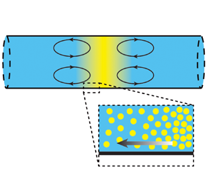
To the best of our knowledge, no theoretical solutions have previously been developed to describe the diffusioosmosis-driven analogue of the Taylor dispersion of solutes. In this study, we take motivations from the works of Alessio et al. (Reference Alessio, Shim, Gupta and Stone2022), Chu et al. (Reference Chu, Garoff, Tilton and Khair2021) and Migacz & Ault (Reference Migacz and Ault2022) and develop analytical solutions for the diffusioosmosis-driven dispersion of a plug of solute in a 2-D channel. We consider a plug of solute that is initially normally distributed in a Gaussian peak at the centre of the channel (see figure 1). As the solute diffuses, the local concentration gradient at the wall drives an effective slip boundary condition via diffusioosmosis that is dependent on the charge of the surface. This slip at the walls drives a recirculating flow in the channel. The recirculation contributes to the advection of the solute transport and introduces cross-stream diffusion, which alters the effective diffusivity of the solute along the channel. In the modelling process, we use a perturbation method to derive analytical solutions to the coupled fluid and solute dynamics. The theoretical analysis is performed for transport in a long, narrow 2-D channel using a 2-D Cartesian coordinate system and in a long, narrow cylindrical pipe using a 2-D axisymmetric cylindrical coordinate system. In § 2, we introduce the governing equations and boundary conditions for both systems. We then apply a perturbation method along with a multiple time-scale analysis to theoretically solve for the fluid and solute dynamics. In § 2.4, we derive the effective diffusivity of the cross-sectionally averaged solute concentration analogously to that of Taylor dispersion. In § 3, we perform numerical simulations to solve for the fluid and solute dynamics and show good agreement with the theoretical predictions. In § 4, we analyse the dispersion behaviour for various conditions and in different time regimes. Finally, while the majority of this analysis focuses on the dispersion of solutes, in § 5, we briefly consider the extension of this modelling approach to coupled particles experiencing diffusiophoresis.

Figure 1. Problem set-up. We consider an initially Gaussian distributed plug of salt with characteristic length  $\ell$ in both (a) 2-D Cartesian coordinates and (b) axisymmetric cylindrical coordinates. Both channels are infinite in the axial direction, and $u_{wall}$ represents the slip velocity at the wall induced by diffusioosmosis.
2. Modelling diffusioosmotic dispersion in a long narrow channel
In this section, we model the coupled fluid and solute transport for a diffusing plug of solute in a channel in the presence of diffusioosmosis-driven recirculation. We consider two configurations, corresponding to planar and cylindrical channels, and describe the flows in these configurations using Cartesian and cylindrical coordinates, respectively. The channel configurations for both systems are shown in figure 1. Initially, we introduce a plug of solute with a Gaussian distribution centred around the origin. In cases when the solute molecules/ions do not interact with the channel walls, the dynamics of the solute transport is governed by simple Brownian diffusion. Here, however, we consider the case where the channel walls have a non-zero surface charge and solute–surface interactions cannot be neglected. The local solute concentration gradient at the channel walls will induce a diffusioosmotic slip velocity boundary condition, which will in turn drive a recirculation in the channel as the solute diffuses. The magnitude of this slip velocity boundary condition is given by 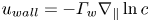 $u_{wall} = -\varGamma _w \nabla _\parallel \ln c$, where $u_{wall}$ is the velocity at the wall in the direction parallel to the wall, and the gradient is taken parallel to the surface. Here, $\varGamma _w$ is the diffusioosmotic mobility coefficient, which is a function of the surface charge of the channel walls, and $c$ is the solute ion concentration. The diffusioosmotic mobility depends on the type of interaction between the solute and surfaces. In the case of electrolyte solutes, the mobility can be positive or negative depending on the zeta potential of the surface and the diffusivity contrast of the ions (Shin et al. Reference Shin, Um, Sabass, Ault, Rahimi, Warren and Stone2016), whereas with neutral solutes the mobility may be strictly positive or negative depending on the type of interaction. For example, with a single neutral solute experiencing an attractive interaction to the surface, the mobility will be strictly positive (Ajdari & Bocquet Reference Ajdari and Bocquet2006).
2.1. Governing equations
The fluid and solute dynamics in the system is governed by the coupled continuity and incompressible Navier–Stokes equations and an advection–diffusion equation for the solute transport. Here, the fluid pressure, density, viscosity and velocity are given respectively by  $p$,
$p$,  $\rho$, $\mu$ and $\boldsymbol {u} = (u,v)\text { or } (u_r,u_z)$. The solute concentration and diffusivity are given by $c(x,y,t)$ and $D_s$, respectively. Here, we consider $Re = {\rho U h}/{\mu } \ll 1$, where $U$ is some characteristic flow velocity in the axial direction; we neglect the influence of gravity, and we treat the fluid dynamics as quasi-steady. The dimensional form of the governing equations is given by
 $$\begin{gather} \nabla^*\cdot\boldsymbol{u}^*=0, \end{gather}$$
 $$\begin{gather}-\nabla^*p^*+\mu\nabla^{*2}\boldsymbol{u}^*=\boldsymbol{0}, \end{gather}$$
 $$\begin{gather}\frac{\partial c^*}{\partial t^*}+ \nabla^*\cdot(\boldsymbol{u^*}c^*)=D_s\nabla^{*2}c^*, \end{gather}$$
where asterisks denote dimensional quantities. The 2-D axisymmetric cylindrical and the 2-D Cartesian cases can be solved similarly and share similar boundary conditions. For the sake of simplicity, we only show the derivation for the 2-D channel flow case in the main text and refer the reader to Appendix B for the derivation for the pipe flow case. The long narrow channel has a height of  $h$ in the Cartesian coordinate system. The channel is infinitely long, and the initial Gaussian solute distribution has a characteristic width of $\ell$, and we will seek solutions in the limit $h\ll \ell$. In addition to facilitating the theoretical solution via the lubrication approximation, this assumption arises from considerations of the parameter regimes needed for Taylor dispersion analysis, as well as considerations about the relative magnitudes of the transport coefficients. In order to use a Taylor dispersion style analysis, the solute must have sufficient time to diffuse across the channel. That is to say, the time scale for solute diffusion across the channel must be small compared with the time scale of solute transfer by convection along the channel, i.e. ${h^2}/{D_s}\ll {\ell }/{u_f}$, where $u_f$ is the flow velocity. For this case of diffusioosmotically driven flow, the fluid velocity scales as the wall slip velocity $u_w\sim {\varGamma _w}/{\ell }$. Thus, for a Taylor dispersion analysis to be valid, we must have ${h^2}/{D_s}\ll {\ell ^2}/{\varGamma _w}$, which gives ${h}/{\ell }\ll \sqrt {{D_s}/{\varGamma _w}}$. Furthermore, for modest zeta potentials we typically have $D_s/\varGamma _w\approx O(1)$ for many common salts, such that we must have ${h}/{\ell }\ll 1$.
To begin, we non-dimensionalize the system of equations as follows:
 \begin{gather}
\begin{gathered}
\displaystyle x = \frac{x^*}{\ell},\quad y = \frac{y^*}{h},\quad u = \frac{u^*}{U},\quad v = \frac{v^*\ell}{Uh},\quad p =
\frac{p^* h^2}{\mu U \ell},\quad \epsilon = \frac{h}{\ell},\notag\\
\displaystyle U = \frac{D_s}{\ell},\quad t = \frac{t^*}{\ell^2/D_s},\end{gathered} \end{gather}
\begin{gather}
\begin{gathered}
\displaystyle x = \frac{x^*}{\ell},\quad y = \frac{y^*}{h},\quad u = \frac{u^*}{U},\quad v = \frac{v^*\ell}{Uh},\quad p =
\frac{p^* h^2}{\mu U \ell},\quad \epsilon = \frac{h}{\ell},\notag\\
\displaystyle U = \frac{D_s}{\ell},\quad t = \frac{t^*}{\ell^2/D_s},\end{gathered} \end{gather}
where  $U=D_s/\ell$ is the characteristic speed of solute diffusion along the channel, and $\ell ^2/D_s$ is the characteristic time of diffusion along the channel. With these scalings, we can rewrite the governing equations (2.1) in non-dimensional form as
 $$\begin{gather} 0 = \frac{\partial u}{\partial x} + \frac{\partial v}{\partial y}, \end{gather}$$
 $$\begin{gather}0 =-\frac{\partial p}{\partial x} + \epsilon^2 \frac{\partial^2 u}{\partial x^2} + \frac{\partial^2 u}{\partial y^2}, \end{gather}$$
 $$\begin{gather}0 =-\frac{\partial p}{\partial y} + \epsilon^4 \frac{\partial^2 v}{\partial x^2} + \epsilon^2 \frac{\partial^2 v}{\partial y^2}, \end{gather}$$
 $$\begin{gather}\epsilon^2\frac{\partial c}{\partial t}+\epsilon^2 u \frac{\partial c}{\partial x} + \epsilon^2 v \frac{\partial c}{\partial y}=\epsilon^2 \frac{\partial^2 c}{\partial x^2} + \frac{\partial^2 c}{\partial y^2}. \end{gather}$$
The solution to the governing equations (2.3) is subject to boundary conditions on the fluid and solute. These boundary conditions can be summarized by
 $$\begin{gather} \text{Quiescent far-field condition: }p=0, u=0,\ c=0 \text{ at } x={\pm}\infty, \end{gather}$$
 $$\begin{gather}\text{No fluid penetration at the walls: } v = 0 \text{ at } y={\pm}\frac{1}{2}, \end{gather}$$
 $$\begin{gather}\text{No-flux conditions at the channel walls: }\frac{\partial c}{\partial y}=0 \text{ at } y={\pm}\frac{1}{2}, \end{gather}$$
 $$\begin{gather}\text{Diffusioosmotic wall slip boundary condition: }u =-\frac{\varGamma_w}{D_s}\frac{\partial \ln c}{\partial x} \text{ at } y={\pm}\frac{1}{2}. \end{gather}$$
The slip boundary condition given by (2.7) is induced by diffusioosmosis, which drives the flow inside the channel. In this study, we assume a constant zeta potential and diffusioosmotic mobility coefficient  $\varGamma _w$. This assumption is needed in order to achieve a final analytical solution, and is a reasonable approximation under many scenarios, as discussed by several recent previous works (see, e.g. Ault et al. Reference Ault, Warren, Shin and Stone2017; Gupta, Shim & Stone Reference Gupta, Shim and Stone2020b; Alessio et al. Reference Alessio, Shim, Gupta and Stone2022; Lee, Lee & Ault Reference Lee, Lee and Ault2022; Migacz & Ault Reference Migacz and Ault2022; Akdeniz, Wood & Lammertink Reference Akdeniz, Wood and Lammertink2023). For typical solutes with modest zeta potentials, the diffusioosmotic mobility, $\varGamma _w$, can range from approximately $-1$ to $1$. We further focus our attention on cases where the initial condition is already spread out relative to the channel width, such that $\epsilon \ll 1$, in which case the lubrication approximation can be used to simplify the governing equations.
2.2. Leading-order fluid dynamics
In our original non-dimensionalization above, we chose a characteristic time scale that is the characteristic time for solute diffusion along the channel  $\ell ^2/D_s$. This corresponds to the slow dynamics of the system. The other important time scale in the system is the characteristic time for solute diffusion across the channel, $h^2/D_s$. This corresponds to the fast dynamics of the system, and the two time scales are separated by a factor of $\epsilon ^2 = h^2/\ell ^2 \ll 1$. Here, in order to develop a solution that is uniformly valid across both the early and late dynamics, we use an approach similar to that of Migacz & Ault (Reference Migacz and Ault2022).
Following this approach, we introduce a multiple time-scale analysis (Bender & Orszag Reference Bender and Orszag1999) in which we introduce a fast-time variable  $T=t/\epsilon ^2$. That is, $T=O(1)$ over dimensional times $\sim h^2/D_s$ corresponding to $t=O(\epsilon ^2)$, whereas $t=O(1)$ on dimensional times $\sim \ell ^2/D_s$. Thus, we can map any time-dependent quantity as
 \begin{equation} f(t)\mapsto f(t,T)\Rightarrow\frac{\partial f}{\partial t}\mapsto \frac{\partial f}{\partial t}+\frac{\partial T}{\partial t}\frac{\partial f}{\partial T} = \frac{\partial f}{\partial t}+\epsilon^{-2}\frac{\partial f}{\partial T}. \end{equation}
With this mapping, the advection–diffusion equation (2.3d), becomes
 \begin{equation} \epsilon^2\frac{\partial c}{\partial t}+\frac{\partial c}{\partial T}+\epsilon^2 u \frac{\partial c}{\partial x} + \epsilon^2 v \frac{\partial c}{\partial y}=\epsilon^2 \frac{\partial^2 c}{\partial x^2} + \frac{\partial^2 c}{\partial y^2}. \end{equation}
We seek an analytical solution of the governing equations as perturbation expansions in the small parameter  $\epsilon ^2$ in the limit of $Re \ll 1$. We seek solutions of the form
 $$\begin{gather} c(x,y,t,T) = c_0(x,y,t,T) + \epsilon^2 c_1(x,y,t,T) + \epsilon^4 c_2(x,y,t,T) + \cdots, \end{gather}$$
 $$\begin{gather}p(x,y,t,T) = p_0(x,y,t,T) + \epsilon^2 p_1(x,y,t,T) + \epsilon^4 p_2(x,y,t,T) + \cdots, \end{gather}$$
 $$\begin{gather}u(x,y,t,T) = u_0(x,y,t,T) + \epsilon^2 u_1(x,y,t,T) + \epsilon^4 u_2(x,y,t,T) + \cdots, \end{gather}$$
 $$\begin{gather}v(x,y,t,T) = v_0(x,y,t,T) + \epsilon^2 v_1(x,y,t,T) + \epsilon^4 v_2(x,y,t,T) +\cdots. \end{gather}$$
The initial condition of the solute concentration is  $c(t=T=0)=\exp (-x^2)$. First, we need to obtain the leading-order velocity and pressure solutions. These can be obtained by substituting equations (2.10) into (2.3), which gives
 $$\begin{gather} 0 = \frac{\partial^2 u_0}{\partial y^2} + \frac{\partial p_0}{\partial x}, \end{gather}$$
 $$\begin{gather}\frac{\partial p_0}{\partial y} = 0, \end{gather}$$
 $$\begin{gather}\frac{\partial u_0}{\partial x} + \frac{\partial v_0}{\partial y} = 0, \end{gather}$$
 $$\begin{gather}\frac{\partial c_0}{\partial T}=\frac{\partial^2 c_0}{\partial y^2}, \end{gather}$$
to leading order. Considering both the initial condition and the no-flux conditions at the channel walls, i.e.  $({\partial c_0}/{\partial y})(\kern0.7pt y=\pm 1/2)=0$, it must be true that $c_0(x,y,t,T)=c_0(x,t)$, with $c_0(t=0)=\exp (-x^2)$. Furthermore, (2.11b) indicates that $p_0$ is only a function of $x$ and $t$.
$t$.
To obtain the leading-order velocities, we first take (2.11a) and solve for  $u_0$, which is subject to the slip boundary condition (2.7). This gives
 \begin{equation} u_0 =-\frac{\varGamma_w}{D_s c_0}\frac{\partial c_0}{\partial x}+\frac{1}{8}(-1+4y^2)\frac{\partial p_0}{\partial x}. \end{equation}
Here,  $u_0$ has a term that includes $p_0(x,t)$, which can be found by considering the conservation of mass and integrating over the channel cross-section $A$, i.e.
 \begin{equation} \frac{1}{A}\iint_A u_0 \,{\rm d} A = 0. \end{equation}
Following this approach,  $p_0(x,t)$, is found to be
 \begin{equation} p_0(x,t) =-\frac{12\varGamma_w}{D_s}\ln c_0. \end{equation}
With this result,  $u_0$ can be simplified and written as
 \begin{equation} u_0(x,y,t) =-\frac{\varGamma_w}{2D_s}\frac{\partial \ln c_0}{\partial x}(-1+12y^2). \end{equation}
To solve for  $v_0(x,y,t)$, we integrate the continuity equation (2.11c) and apply the boundary condition given by (2.5). This gives the leading-order $y$-component of velocity to be
 \begin{equation} v_0(x,y,t) =-\frac{\varGamma_w}{2D_s}\frac{\partial^2 \ln c_0}{\partial x^2}(1-4y^2)y. \end{equation}
As mentioned, the equivalent results for the flow in a cylindrical pipe can be found in Appendix B.
2.3. Higher-order solute transport
The higher-order solute concentration results from diffusioosmosis, which causes the deviation from pure diffusion. Using the leading-order velocity profiles found above, we seek a solution for the higher-order solute dynamics from (2.3d). Substituting our asymptotic expansion into the advection–diffusion equation (2.9), we find, to leading order, that
 \begin{equation} \frac{\partial c_1}{\partial T} + \frac{\partial c_0}{\partial t}+u_0\frac{\partial c_0}{\partial x} = \frac{\partial^2 c_0}{\partial x^2} + \frac{\partial^2 c_1}{\partial y^2}. \end{equation}
The term involving  $v$ has disappeared since ${\partial c_0}/{\partial y} = 0$. To find a solution to this problem, we first consider long times such that $T\gg 1$, but $t$ is finite. In this limit, ${\partial c_1}/{\partial T}$ is small. Then, averaging equation (2.17) over the channel cross-section gives
 \begin{equation} \frac{\partial c_0}{\partial t} = \frac{\partial^2 c_0}{\partial x^2}. \end{equation}
The solution to this problem is given by
 \begin{equation} c_0(x,t)=\frac{1}{\sqrt{1+4t}}\exp \left(-\frac{x^2}{1+4t}\right), \end{equation}
which has been presented previously by Chu et al. (Reference Chu, Garoff, Tilton and Khair2020) and Gupta et al. (Reference Gupta, Shim and Stone2020b). The advection–diffusion equation (2.17) can then be simplified to
 \begin{equation} \frac{\partial c_1}{\partial T} - \frac{\varGamma_w}{2D_s}\frac{\partial \ln c_0}{\partial x}(-1+12y^2)\frac{\partial c_0}{\partial x}=\frac{\partial^2 c_1}{\partial y^2}, \end{equation}
subject to the initial condition  $c_1(t=T=0)=0$. To solve this, we note that at long times the fast-time dynamics should have all decayed such that the time derivative term can be ignored, and the equation can be integrated to yield
 \begin{equation} c_1(T\rightarrow\infty)\sim c_1^\infty(x,y,t)=-\frac{y^2}{4c_0}\frac{\varGamma_w}{Ds}(-1+2y^2)\left(\frac{\partial c_0}{\partial x}\right)^2+B(x,t), \end{equation}
where  $B(x,t)$ is a yet unknown function that results from the integration. To solve for $B(x,t)$, we substitute (2.21) into (2.9), and take the cross-sectional average of the equation, which gives
 \begin{align} \frac{\partial^2 B}{\partial x^2} =-\frac{\varGamma_w}{D_s}\frac{{\rm e}^{-{x^2}/({1+4t})}}{420(1 +4t)^{9/2}}\left[49(1+4t)^2-48\frac{\varGamma_w}{D_s}(1+4t)x^2 +32\frac{\varGamma_w}{D_s}x^4 \right]+\frac{\partial B}{\partial t}. \end{align}
Note that, until now, we have left the results in terms of a general  $c_0$, but here and in the solution for $B$ below, we have substituted the specific solution for $c_0$ shown above since it is needed to solve the (2.22) using the Fourier transform approach. This procedure can be repeated for other arbitrary initial conditions as needed. Using a Fourier transform approach, $B(x,t)$ can be found to be
 \begin{align} B={\,-\,}\frac{\varGamma_w}{D_s}\frac{{\rm e}^{-{x^2}/{\alpha}}}{840 \alpha^{9/2}}\left(\!49(\alpha x)^2{\,-\,}16\frac{\varGamma_w}{D_s}t (3\alpha^2{\,-\,}12\alpha x^2{\,+\,}4x^4 ){\,+\,}12\frac{\varGamma_w}{D_s} \alpha^2(\alpha{\,-\,}2x^2)\ln(\alpha)\!\right), \end{align}
where  $\alpha (t)=1+4t$. Note that $c_1^\infty$ only depends on the slow time $t$ and not the fast time $T$. It does not satisfy the initial condition, so it is not yet the full solution for the higher-order solute dynamics. We seek a solution of the form $c_1(x,y,t,T) = c_1^\infty (x,y,t)+\hat {c}_1(x,y,t,T)$. Substituting into (2.20), we find
 \begin{equation} \frac{\partial \hat{c}_1}{\partial T} = \frac{\partial^2 \hat{c}_1}{\partial y^2},\quad \text{with the initial condition }\hat{c}_1(T=0)=-c_1^\infty(t=0), \end{equation}
the solution to which is
 \begin{equation} \hat{c}_1 = \left. -\frac{\varGamma_w}{4c_0D_s}\left(\frac{\partial c_0}{\partial x}\right)^2\right|_{t=0}\sum_{n=1}^\infty \frac{6(-1)^n}{n^4{\rm \pi}^4}\, {\rm e}^{-(2n{\rm \pi})^2 T}\cos 2n{\rm \pi} y. \end{equation}
We can then construct a composite solution  $c_1=c_1^\infty +\hat {c}_1$, which is valid for all $t$. The solution of $c_1$ can be verified to satisfy the conservation of mass by considering
 \begin{equation} \int^\infty_{-\infty}\int^{1/2}_{-1/2} c_1(x,y,t,T)\,{\rm d} y\,{\rm d}\kern0.7pt x = 0. \end{equation}
Once again, analogous results for the coupled dynamics in a cylindrical pipe geometry can be found in Appendix B. Even though the theoretical solutions are formally valid for  $\epsilon \ll 1$, the solution still works well even for $\epsilon = O(1)$, for example, when the initial condition is compact, which we will show in the later sections.
2.4. Effective diffusivities
As mentioned, the diffusioosmotic slip flow at the channel walls induces a recirculating flow that drives an advective transport of the solute, altering the effective diffusivity of its transport as it diffuses along the channel. Here, we seek to characterize the effective diffusivity of this transport by deriving a 1-D transport equation for the cross-sectionally averaged solute transport. This approach is analogous to that of Taylor (Reference Taylor1953) and Aris (Reference Aris1956) in their famous work on solute dispersion in the presence of pressure-driven shear flow (see also, e.g. Aminian et al. Reference Aminian, Bernardi, Camassa, Harris and McLaughlin2016; Alessio et al. Reference Alessio, Shim, Gupta and Stone2022).
To begin, we define  $c'(x,y,t)$ as the deviation of the solute concentration from its cross-sectionally averaged value $\overline {c(x,y,t)}$, where overbars are used to denote the average over a cross-section
 \begin{equation} c'(x,y,t) = c(x,y,t) - \overline{c(x,t)}. \end{equation}
Substituting this definition into the solute advection–diffusion equation gives
 \begin{equation} \frac{\partial \bar{c}}{\partial t}+\frac{\partial c'}{\partial t}+u \frac{\partial c'}{\partial x} +u \frac{\partial \bar{c}}{\partial x}+ v \frac{\partial c'}{\partial y}=\frac{\partial^2 \bar{c}}{\partial x^2} + \frac{\partial^2 c'}{\partial x^2}+\frac{1}{\epsilon^2}\frac{\partial^2 c'}{\partial y^2}. \end{equation}
Next, averaging this equation over the cross-section gives
 \begin{equation} \frac{\partial \bar{c}}{\partial t} + \overline{u \frac{\partial c'}{\partial x}} + \overline{v \frac{\partial c'}{\partial y}} = \frac{\partial^2 \bar{c}}{\partial x^2}. \end{equation}
Here, substituting in our solutions for  $u$ and $v$ from above, this can be rewritten into a 1-D diffusion equation with a known forcing term given by
 \begin{equation} \frac{\partial \bar{c}}{\partial t} + \frac{\partial}{\partial x}\left[\left(\frac{\varGamma_w}{D_s}\right)^2\frac{\epsilon^2}{210} \left(\frac{\partial}{\partial x}\ln c_0 \right)^2\frac{\partial c_0}{\partial x} \right] = \frac{\partial^2 \bar{c}}{\partial x^2}. \end{equation}
This equation can easily be solved numerically. For the purposes of making an analogy to the classic Taylor dispersion problem, this can be rewritten into a 1-D pure diffusion problem by recognizing that  ${\partial c_0}/{\partial x}-{\partial \bar {c}}/{\partial x}=O(\epsilon ^2)$, which gives
 \begin{equation} \frac{\partial \bar{c}}{\partial t} = \frac{\partial}{\partial x}\left(D_{eff} \frac{\partial \bar{c}}{\partial x}\right), \end{equation}
where the effective diffusivity  $D_{eff}$ is given by
 \begin{equation} D_{eff} =1+\left(\frac{\varGamma_w}{D_s}\right)^2 \frac{\epsilon^2}{210}\left(\frac{\partial}{\partial x}\ln c_0\right)^2 +O(\epsilon^4). \end{equation}
 Equation (2.32) is similar to what Alessio et al. (Reference Alessio, Shim, Gupta and Stone2022) presented. From (2.32), we see that, to leading order, the effective non-dimensional diffusivity is  $D_{eff}=1$, and the effects of diffusioosmosis on the dispersion are $O(\epsilon ^2)$. That is, as $\epsilon \rightarrow 0$, the initial condition of the solute plug becomes more spread out, the concentration gradients get weaker and the diffusioosmosis becomes negligible. The same behaviour occurs as $t\rightarrow \infty$ as the solute spreads out over long times. Furthermore, the contribution from diffusioosmosis is also $O((\varGamma _w/D_s)^2)$. Thus, despite the nonlinearity of the diffusioosmotic boundary condition, flipping the sign of $\varGamma _w$ (and thus the direction of the recirculation) results in the same effective diffusivity. This result may at first be surprising upon noticing that $c_1$ depends on both $\varGamma _w/D_s$ and $(\varGamma _w/D_s)^2$, such that the deviations in the solute concentration from $c_0$ are not mirror images of each other when the sign of the mobility is flipped (this will be visualized below in figure 7). However, this dependence arises from the symmetry and area-averaging nature of the analysis, and is essentially analogous to the idea from Taylor dispersion that the effective diffusivity is independent of the pressure-driven flow direction.
Following a similar approach and using the results from Appendix B, the analogous averaged transport equation for the cylindrical pipe case is given by
 \begin{equation} \frac{\partial \bar{c}}{\partial t} + \frac{\partial}{\partial z}\left[\left(\frac{\varGamma_w}{D_s}\right)^2\frac{\epsilon^2}{48} \left(\frac{\partial}{\partial z}\ln c_0 \right)^2\frac{\partial c_0}{\partial z} \right] = \frac{\partial^2 \bar{c}}{\partial z^2}. \end{equation}
This can also be written into a form analogous to Taylor dispersion as
 \begin{equation} \frac{\partial \bar{c}}{\partial t} = \frac{\partial}{\partial z}\left(D_{eff} \frac{\partial \bar{c}}{\partial z}\right), \end{equation}
where the effective diffusivity  $D_{eff}$ to leading order is given by
 \begin{equation} D_{eff} =1+\left(\frac{\varGamma_w}{D_s}\right)^2 \frac{\epsilon^2}{48}\left(\frac{\partial}{\partial z}\ln c_0\right)^2+O(\epsilon^4). \end{equation}
Note that the contribution of diffusioosmosis to the effective diffusivity in a 2-D channel flow is a factor of 48/210 weaker than in a cylindrical pipe system. This is a consequence of the fact that, for a given slip velocity at the walls, the centreline velocity in a cylindrical pipe must be greater than in a 2-D channel flow, leading to greater velocity gradients, greater distortion of the solute profile and a greater contribution to the effective diffusivity enhancement. Using these effective diffusivities along with the 1-D diffusion equation, the evolution of the cross-sectionally averaged solute concentration is quite efficient to compute numerically.
3. Numerical methods
To validate the theoretical results above, we performed numerical simulations for the coupled transport in both geometries. In this section, we describe the numerical methods used and show that the theoretical results above accurately match the numerical results. The velocity profiles are solved for the 2-D channel flow case using a Fourier transform approach and for the cylindrical pipe flow case using a multigrid relaxation approach. Because we are dealing with the low Reynolds number regime and the fluid dynamics can be treated as quasi-steady, the numerical approach can be outlined as follows. First, we initialize the solute concentration to the previously described Gaussian distribution. We then solve for the quasi-steady velocity profile using either a numerical multigrid relaxation approach or the theoretical Fourier transform approach. Next, using the determined velocity profiles, we update the solute concentration profile using a numerical solution of the governing advection–diffusion equation. This procedure is then repeated until the final time.
3.1. Velocity solver
For the case of incompressible Newtonian Stokes flow, the governing equations can be simplified to a biharmonic equation for the streamfunction,  $\psi$, which is given by
 \begin{equation} \nabla^4 \psi = 0. \end{equation}
This is a convenient formulation, as it allows for the solution of the velocity profiles without needing to solve for the pressure. In the Cartesian coordinate system, a Fourier transform approach can be used to greatly accelerate the numerical solution of this equation. In particular, the biharmonic equation can be Fourier transformed in the  $x$ direction as
 \begin{equation} k^4\hat{\psi}(k,y)-2k^2\frac{\partial^2 \hat{\psi}(k,y)}{\partial y^2}+\frac{\partial^4 \hat{\psi}(k,y)}{\partial y^4}=0. \end{equation}
Here, we ignore the functional dependence of  $\psi$ on time because the velocity can be treated as quasi-steady. The boundary conditions for (3.2) are $\hat {\psi }(k,0)=0$, ${\partial ^2 \hat {\psi }}/{\partial y^2}|_{y = 0} = 0$, $\hat {\psi }(k,\pm 1/2)=0$ and ${\partial \hat {\psi }}/{\partial y}|_{y=\pm 1/2}=\hat {u}_{wall}$. Here, $\hat {u}_{wall}$ can be found by using the fast Fourier transform, and $\psi$ can be found by using the inverse fast Fourier transform of $\hat {\psi }$. Finally, the velocity components can be obtained directly from $\psi$ using
 \begin{equation} u = \frac{\partial \psi}{\partial y}, \quad v =-\frac{\partial \psi}{\partial x}. \end{equation}
For the case in cylindrical coordinates, we have not found a similar approach to using a Fourier transform to rapidly solve the biharmonic equation, so we instead do this directly using a multigrid solution to a set of coupled Poisson equations, and we then use the direct finite difference method to solve for the velocity. In particular, the biharmonic equation can be written as follows:
 $$\begin{gather} D^2 \psi = r\frac{\partial}{\partial r}\left( \frac{1}{r}\frac{\partial \psi}{\partial r}\right) + \frac{\partial^2 \psi}{\partial z^2}=\phi, \end{gather}$$
 $$\begin{gather}D^2 \phi = r\frac{\partial}{\partial r}\left( \frac{1}{r}\frac{\partial \phi}{\partial r}\right) + \frac{\partial^2 \phi}{\partial z^2}=0, \end{gather}$$
where  $D^2$ is a special operator in cylindrical coordinates that is useful for the biharmonic equation, which is given by $D^2 = r({\partial }/{\partial r})(({1}/{r})({\partial }/{\partial r})) + {\partial ^2}/{\partial z^2}$ (Stimson & Jeffery Reference Stimson and Jeffery1926; Brenner Reference Brenner1961). Here, $\phi =D^2\psi$ is defined in (3.4a), and is a placeholder variable that is needed so both equations can be solved simultaneously using the multigrid method. The wall has boundary conditions of $({1}/{r})({\partial \psi }/{\partial r}) = u_{wall}$ and $\phi = -({1}/{r})({\partial \psi }/{\partial r}) + {\partial ^2 \psi }/{\partial r^2}$. All of the other boundaries have $\psi = 0$ and $\phi = 0$ because of symmetry conditions and no-flux conditions at the end of the channel.
This set of coupled Poisson equations is solved by using the Gauss–Seidel relaxation method with second-order accuracy in space and time for both governing equations and boundary conditions. As mentioned, the multigrid approach was used to rapidly accelerate the convergence of this iterative approach.
3.2. Concentration solver
The solute concentration profiles can be numerically solved using the advection–diffusion equation. We use a finite difference with the approximate factorization method to solve the advection–diffusion equation for both geometries (Moin Reference Moin2010). Numerical details of the concentration solver are given in Appendix A. Note that in all cases we add a small offset background concentration of  $10^{-7}$ to prevent the so-called ‘ballistic motion’ described by Gupta et al. (Reference Gupta, Shim and Stone2020b), which represents the background ion concentration typically present in solution due to dissolved CO $_2$ or other factors. In this section, we have developed and presented the numerical methods used for both systems. In the following section, we explore the range of results and the physical evolution of such systems with numerical validation, and we show that the cross-sectionally averaged approach closely approximates the results of fully 2-D simulations and can greatly simplify the analysis as in the case of Taylor dispersion.
4. Results
To begin, we first use the numerical simulations to validate the theoretical predictions. An example comparison between the numerical and theoretical results is shown in figure 2. The analytical predictions of velocities in the parallel-plate channel are calculated by using (2.15) and (2.16), and those in the cylindrical channel are calculated from (B13) and (B14). Results are compared for  $\varGamma _w/D_s = 1$ and $\epsilon =0.1$ at $t=0.2$. With a positive diffusioosmotic mobility, the wall slip velocity is away from the peak solute concentration, driving flow away from the centreplane ( $x=0$ or $z=0$) at the walls and towards the centreplane along the channel centreline ( $\kern0.7pt y=0$ or $r=0$). The theoretical and numerical results agree well. One feature of the results to notice is that the velocity along the centreline in the cylindrical case is enhanced relative to the Cartesian case. We will see later how this alters the effective dispersion in such configurations. Figure 3 shows the comparison between (a,c) numerical simulations and (b,d) theoretical predictions of the higher-order solute concentration in the parallel-plate (a,b) and the cylindrical (c,d) channels, respectively. Here, the results are plotted over one quarter of the domain due to symmetry. The comparison is again calculated with $\varGamma _w/D_s = 1$ and $\epsilon = 0.1$, and the results demonstrate that the numerical results closely match the theoretical predictions.
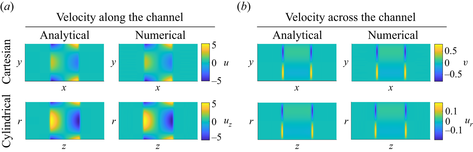
Figure 2. The comparison between numerical and theoretical velocity predictions in both coordinate systems. The recirculating velocity is due to the diffusioosmotic motion at the channel walls, which is driven by the  $u_{{wall}} = -({\varGamma _w}/{D_s})({\partial \ln c}/{\partial x})$ or $u_{{wall}} = -({\varGamma _w}/{D_s})({\partial \ln c}/{\partial z})$ slip boundary condition for the Cartesian and cylindrical coordinate systems, respectively. Results are computed for $\varGamma _w/D_s = 1$ and $\epsilon =0.1$ at $t=0.2$.

Figure 3. Evolution of the higher-order solute concentration in both the Cartesian (a,b) and cylindrical (c,d) geometries. This illustrates the deviation of the solute concentration profile from the purely 1-D dynamics and represents the role of the diffusioosmotic dispersion. The panels with  $c_{num}-c_0$ represent the numerically computed solute evolution minus the theoretical 1-D solution, and panels with $\epsilon ^2 c_1$ show the theoretically calculated higher-order solute profile. Results are presented over time for $\varGamma _w/D_s = 1$ and $\epsilon =0.1$.
Having validated the theoretical solutions using numerical simulations, we now provide a detailed examination of the diffusioosmotic dispersion process. We first consider the early-time dynamics of the system over which the initial deviation of the solute profile from the purely 1-D dynamics forms. Figure 4 illustrates this early-time dynamics by presenting visualizations of both  $\hat {c}_1$, $c_1^\infty$, and $c_1$ in the early-time regime for times up to $t=1\times 10^{-3}$ with $\epsilon =0.1$ and $\varGamma _w/D_s = 1$. Recall that the fast time scale corresponds to the characteristic time for diffusion to occur across the channel and is represented by $\hat {c}_1$ from (2.25). In contrast, the slow time scale corresponds to the diffusion along the channel and is represented by $c_1^\infty$ from (2.21). Here, $c_1$ is the total deviation of the solute concentration profile from the purely 1-D dynamics and is formed by the sum of both $c_1^\infty$ and $\widehat {c_1}$. As can be seen, the purpose of $\hat {c}_1$ is to cancel out the initial condition of $c_1^\infty$ such that the initial condition of $c_1$ can be zero. Then, in this example, $\hat {c}_1$ has almost entirely decayed by $t=10^{-3}$ after which the solution is dominated by the slow-time dynamics.

Figure 4. Components of the higher-order solute contribution during the early-time regime. Results are calculated for  $\varGamma _w/D_s = 1$ and $\epsilon = 0.1$ up to a time of $t=1\times 10^{-3}$. Here, $c_1^\infty$ is calculated from (2.21) and corresponds to the long-time solution from the multiple time-scale analysis. The $\hat {c}_1$ component is calculated from (2.25) and corresponds to the fast-time dynamics that is required to satisfy the initial condition. The total higher-order solute profile is then given by $c_1 = c_1^\infty +\hat {c}_1$. The contribution due to the fast-time dynamics decays over the time scale for solute diffusion across the channel, and the long-time contribution decays over the time scale for diffusion along the channel.
The early-time dynamics is expected to decay over the time scale  $\epsilon ^2$. This can be verified by plotting the peak value of $\hat {c}_1$ over a range of mobilities and $\epsilon$ values, which is shown in figure 5. Solid dots correspond to the results of 2-D simulations which are calculated as $\hat {c}_{num} = (c-c_0)/\epsilon ^2-c_{1,{theory}}^\infty$. Specifically, figure 5 $(\textit {a})$ shows the peak of $\widehat {c_1}$ with $\epsilon = 0.1$ at various $\varGamma _w/D_s$ values. As can be seen, higher $\varGamma _w/D_s$ values correspond to larger peak $\hat {c}_1$ values, reflecting the enhanced dispersion in those cases. For all $\varGamma _w/D_s$, the peak $\hat {c}_1$ values have all apparently decayed before $t$ reaches $\epsilon ^2=10^{-2}$. Figure 5(b) extends these results by considering cases with different $\epsilon$ values at a constant $\varGamma _w/D_s=1$. Here, the dashed lines are the locations where $t=\epsilon ^2$. As expected, in every case the peak $\hat {c}_1$ value vanishes over the time scale $t=O(\epsilon ^2)$ as predicted by the theory.

Figure 5. Evolution of the peak values of  $\hat {c}_1$ in the channel over time as functions of (a) $\varGamma _w/D_s$ for fixed $\epsilon =0.1$ and (b) $\epsilon$ for fixed $\varGamma _w/D_s=1$. Solid dots indicate the 2-D numerical simulation results, $\hat {c}_{num} = (c-c_0)/\epsilon ^2-c_{1,{theory}}^\infty$. The theoretical predictions show an excellent agreement with the 2-D numerical simulation. The dashed lines correspond to the time when $t=\epsilon ^2$. Recall that $\hat {c}_1$ represents the fast-time dynamics in the system corresponding to solute diffusion across the channel and is expected to decay over the time scale $t\sim \epsilon ^2$ as shown. In (a), the increased magnitude with increasing $\varGamma _w/D_s$ reflects the enhanced dispersion with stronger diffusioosmosis.
In § 2, we developed a theoretical model for the higher-order correction to the solute concentration profile due to diffusioosmosis. As discussed, the diffusioosmotic slip flow drives a recirculating flow in the channel that alters the transport of the solute. The vorticity and recirculating fluid flow in the channels are shown in figure 6 at  $t=1$ for both coordinate systems. Here, (a) and (c) show the non-dimensional vorticity on the cross-section for the parallel-plate and cylindrical channels, respectively, with $\varGamma _w/D_s=1$. Streamlines illustrating the recirculation on the cross-section are superposed on top of the colour map. Panels (b) and (d) show the same non-dimensional vorticity data but with scaled velocity vector maps superposed instead. With $\varGamma _w/D_s = 1$, the diffusioosmosis at the channel walls drives a slip flow away from the centreplane, driving a recirculating flow that is towards the centreplane along the channel centreline. The flow directions and the signs of the vorticity will be reversed in cases with negative mobilities.

Figure 6. Non-dimensional vorticity and flow visualizations of the recirculation driven by diffusioosmosis for  $\varGamma _w/D_s=1$ at $t=1$. Panels (a) and (c) correspond to the 2-D channel flow case, and (b) and (d) correspond to the axisymmetric pipe flow case. Streamlines highlighting the recirculation zones are shown in (a) and (b), and velocity vector maps are shown in (c) and (d). Results correspond to the leading-order velocity profiles and thus are independent of $\epsilon$.
Next, we visualize the higher-order solute dynamics on the cross-section to better understand the role of the diffusioosmotic dispersion on the solute transport. Figure 7 shows the theoretical values of  $c_1$ for both parallel-plate (a) and cylindrical (b) channels as functions of $\varGamma _w/D_s$ at a fixed time of $t=1$. In order to interpret the figure, recall that positive $\varGamma _w$ values correspond to slip flow away from the centreplane along the walls and towards the centreplane along the centreline of the channel, while negative $\varGamma _w$ values correspond to flows that recirculate in the opposite direction. Regions of positive $c_1$ (red) indicate locations that have increased solute concentration relative to the 1-D pure diffusion case ( $c_0$), and regions of negative $c_1$ (blue) have relatively less concentration relative to $c_0$. We can interpret the formation of these regions as follows. For example, consider the case with $\varGamma _w/D_s=1$ in the parallel-plate channel. Along the channel walls, the flow is away from the centreplane $x=0$, pulling the relatively higher concentration fluid away from $x=0$ and enhancing the solute concentration somewhat away from the centreplane. This is enhanced by the recirculating nature of the flow that also pulls flow away from the centreline of the channel and towards the walls. Along the centreline, the flow is towards the centreplane, pulling relatively lower concentration fluid towards the centreplane and resulting in a depletion region. These effects are flipped in the case of negative $\varGamma _w/D_s$. From figure 7, it is apparent that $c_1$ is not symmetric in $\varGamma _w/D_s$, as mentioned above. That is, the figure shows that $c_1(\varGamma _w/D_s=-1) \neq -c_1(\varGamma _w/D_s=1)$. Nonetheless, the contribution of diffusioosmosis to the effective diffusivity is $O(\varGamma _w/D_s)^2$, which again arises due to the fact that flipping the sign of $\varGamma _w$ simply flips the sign of the velocity along with the fact that the results are area averaged. One last point to note is that the cylindrical case has relatively greater solute depletion and enhancement along the channel centreline due to the relatively greater centreline velocity in a cylindrical pipe compared with a 2-D channel flow for the same wall slip velocity.

Figure 7. Higher-order solute concentration profiles  $c_1$ as functions of $\varGamma _w/D_s$ at $t=1$. Panel (a) corresponds to the 2-D Cartesian channel flow system and is calculated from (2.21), while panel (b) corresponds to the axisymmetric pipe flow case and is calculated from (B19). In both panels, the vertical coordinate ( $\kern0.7pt y$ or $r$) has been stretched by a factor of 2 for visualization purposes; (a) $c_1$ in Cartesian coordinates at $t=1$ and (b) $c_1$ in cylindrical coordinates at $t=1$.
Next, we visualize the long-time behaviour of the solute concentration profile as modelled by  $c_1^\infty$. Recall that, for $t>O(\epsilon ^2)$, the higher-order solute profile is $c_1\approx c_1^\infty$, as $\hat {c}_1$ has already decayed. The long-time results are shown in figure 8 for times up to $t=1000$ with $\varGamma _w/D_s=1$. Here, the horizontal axis is scaled by $\sqrt {1+4t}$, since this represents the rate of spread of $c_0$ along the channel. Recall that, with our non-dimensionalization, this corresponds to 1000 times the characteristic time for diffusion along the channel, such that the initial pulse of solute has well decayed by this time. As shown in the figure, over long times, the higher-order solute profile also spreads significantly in the axial direction, retaining qualitatively the same shape, and ultimately decaying. As the initial pulse of solute decays, the concentration gradient at the walls likewise decays such that the diffusioosmosis and recirculating flow also decay with time, leading to the ultimate decay of $c_1$. Here, panel (a) corresponds to the 2-D channel flow case, and panel (b) corresponds to the axisymmetric pipe flow case. The only significant notable difference between the two cases is that the magnitude of the higher-order solute concentration is a factor of 4–5 higher for the cylindrical case. As mentioned, this is due to the relatively greater centreline velocity in the axisymmetric geometry, which yields greater velocity gradients and enhanced dispersion.

Figure 8. Long-time behaviour of the higher-order solute concentration  $c_1$ with $\varGamma _w/D_s=1$ for times up to $t=1000$. Panel (a) corresponds to the 2-D channel flow case, and panel (b) corresponds to the axisymmetric pipe flow case. In both cases, the axial coordinate is scaled by $\sqrt {1+4t}$, demonstrating that the higher-order solute effects spread at the same rate as $c_0$. As time proceeds, the solute concentration gradient at the walls decreases as the solute pulse spreads out, leading to decreased diffusioosmosis at the channel walls, less recirculation and thus less dispersion. Ultimately, the higher-order profile smears out by diffusion, and the dynamics approaches that of pure diffusion.
Before proceeding to investigate the cross-sectionally averaged dynamics, we consider the effect of varying  $\epsilon$ and the breakdown of the theoretical solution at large $\epsilon$. Figure 9 shows the theoretical and numerical predictions of the higher-order solute concentration profiles in the parallel-plate channel with $\varGamma _w/D_s=1$ at $t=1$. As shown above, the theoretical predictions show good agreement with the numerical results in the limit of small $\epsilon$. Here, we see that reasonable quantitative agreement between the theory and simulations exists up to approximately $\epsilon =2$, above which the theoretical predictions break down. In particular, as can be seen for $\epsilon =10$ in figure 9, the numerical results show a much more uniform depletion along the channel centreline near $x=0$ compared with the theoretical results.

Figure 9. Higher-order solute concentration profiles  $\epsilon ^2c_1$ in the parallel-plate channel with $\varGamma _w/D_s=1$ at $t=1$. Panel (a) corresponds to the theoretical predictions of $\epsilon ^2c_1$ and is calculated from (2.21) and panel (b) corresponds to the numerical simulation of $c - c_0$. As can be seen, the theoretical results appear to break down above approximately $\epsilon =2$.
Finally, following the strategy of Taylor and Aris, we consider the dynamics of the cross-sectionally averaged concentration profile. In § 2.4, we derived a cross-sectionally averaged concentration equation that can be used to model the net effects of diffusioosmotic dispersion. These equations are relatively simpler 1-D diffusion equations with an effective diffusion coefficient that depends on the channel geometry and captures the effects of the dispersion. Unlike in the relatively simpler case of pure Taylor dispersion, here, the effective diffusivity is no longer a constant but rather a function of both axial position in the channel and time, as the net effects of the dispersion evolve with time and space. Thus, several methods are available for characterizing the cross-sectionally averaged solute dynamics. First, this 1-D variable diffusivity model can be easily numerically integrated in time to yield the dynamics. Second, the results of the 2-D numerical simulations can be averaged over the cross-section. Finally, the theoretical results for  $c=c_0+\epsilon ^2 c_1$ can be averaged over the cross-section to yield the theoretical leading-order dynamics. All of these approaches should be expected to match up to $O(\epsilon ^2)$. A visualization of the cross-sectionally averaged solute dynamics is shown in figure 10 for the parallel-plate channel. Here, the results are the deviation of the cross-sectionally averaged solute concentration from the 1-D results i.e. $\bar {c}-c_0$. Figure 10(a) shows results as a function of $|\varGamma _w/D_s|$ with $\epsilon =0.1$ and $t=1$. The solid lines indicate the theoretical predictions. The square markers correspond to the results of numerically solving the 1-D forced diffusion equation given by (2.30). The star markers represent the results of averaging the 2-D numerical simulation results over the cross-section. All three methods show close agreement. Recall that in the effective diffusivity coefficients derived in § 2.4, the contribution from diffusioosmosis is $O(\varGamma _w/D_s)^2$, such that the sign of the mobility does not affect the cross-sectionally averaged evolution.

Figure 10. Evolution of the cross-sectionally averaged solute dynamics for the 2-D channel flow case. Results show the cross-sectionally averaged solute concentration  $\bar {c}$ minus the results from pure diffusion $c_0$. (a) Results as a function of $|\varGamma _w/D_s|$ with $\epsilon =0.1$ and $t=1$. Solid lines correspond to the cross-sectionally averaged theoretical results developed in § 2.4. Square symbols correspond to the numerical solution of the 1-D forced diffusion equation given by (2.30). Star symbols indicate the cross-sectional average of the full 2-D numerical simulations. All three methods of calculating $\bar {c}-c_0$ show excellent agreement at small $\epsilon$.(b) Results as a function of $\epsilon$ with $|\varGamma _w/D_s|=1$ and $t=1$. Solid lines correspond to numerical results, and square markers indicate theoretical predictions. The errors in the theoretical predictions manifest graphically for $\epsilon \geq 2$. (c) Results over time with fixed $\varGamma _w/D_s=1$ and $\epsilon =0.1$. Solid lines correspond to the theoretical predictions, and star symbols indicate the cross-sectional average of the full 2-D numerical simulations. (d) Numerical results of the 1-D model over time with fixed $\varGamma _w/D_s=1$ and $\epsilon =10$.
However, increasing the magnitude of  $\varGamma _w/D_s$ enhances the diffusioosmosis relative to the solute diffusion, leading to greater dispersion and greater deviations from $c_0$. Figure 10(b) shows the cross-sectionally averaged solute concentration as a function of $\epsilon$ with $|\varGamma _w/D_s|=1$ and $t=1$. The solid lines indicate the numerical simulations, and the square markers correspond to the theoretical predictions. As the value of $\epsilon$ increases, the magnitude of diffusioosmotic dispersion increases, enhancing the deviations from the pure diffusion case. The theoretical predictions show a good agreement with the simulations up to approximately $\epsilon =1$. As shown, as $\epsilon$ increases beyond 1, the results of the 1-D model break down, and errors between the numerical simulations manifest quickly. This breakdown is consistent with the description provided above about the assumption $h\ll \ell$. That is, if $h/\ell$ is not small, this implies that the solute does not have sufficient time to diffuse across the cross-section, and a Taylor diffusion style 1-D analysis is inappropriate. Figure 10(c,d) present the cross-sectionally averaged concentration profile as a function of time. Figure 10(c) shows the theoretical (solid lines) and numerical (star symbols) predictions of the cross-sectionally averaged solute concentration for constant $\varGamma _w/D_s=1$ and $\epsilon =0.1$ and (d) shows the cross-sectionally averaged solute concentration from numerical simulations for constant $\varGamma _w/D_s=1$ and $\epsilon =10$. As time progresses, a relative depletion zone forms near the channel centre that is balanced by accumulation regions to the left and right of the solute peak. Note that the depletion at $x=0$ does not form quite as quickly as that near $x=0$, resulting in a small bump that decays with time. This is due to the fact that the axial concentration gradient is zero at $x=0$ due to symmetry, such that the wall slip velocity and any recirculating flow is negligible very near the centreplane. Thus, some time is still required for the solute to diffuse and adjust.
In addition, we study the width of the spread of the cross-sectionally averaged concentration profiles. Here, we define the width of the solute distribution as  $\mathcal {L}_{99}$, which corresponds to the axial position ( $x$ or $z$), where the concentration has decayed by 99 % of its current peak value. Numerical results for a range of $\epsilon$ values are shown in figure 11 and compared with the theoretical predictions. Panel (a) shows the rescaled width of the concentration distributions as a function of time with constant $\varGamma _w/D_s=1$ for different values of $\epsilon$. The coloured markers represent the numerical results of solute concentration, and the solid and light blue dashed lines correspond to theoretical predictions of the distribution width of $c0+\epsilon ^2c_1^\infty$ and $c_0$, respectively. Here, the distribution widths are rescaled by $\sqrt {1+4t}$, which represents the expected spreading rate of $c_0$. As can be seen, the results tend towards constant values, indicating that the spread of the higher-order solute profile is set by the spread of $c_0$. This is due to the fact that while $c_0$ becomes small at the edge of the distribution, the gradient of the logarithm of $c_0$ may remain large, allowing the diffusioosmotic dispersion to act over a relatively wider distribution. As $\epsilon$ increases, the width of the higher-order solute distribution increases. Figure 11(b) shows $\mathcal {L}_{99}$ as a function of $\epsilon$ with constant $\varGamma _w/D_s=1$ at a fixed time of $t=1$. Here, the theoretical predictions of $c_0+\epsilon ^2c_1^\infty$ and $c_0$ are shown as a solid line and a dashed line, respectively. The symbol markers correspond to the numerical results. At a given time, the width of the distribution increases with a larger $\epsilon$ value. The theoretical predictions show a good agreement with numerical simulation for $\epsilon <1$, and the error between simulations and theory for this metric remains less than 10 % even at $\epsilon = 10$.

Figure 11. Rescaled width of the cross-sectionally averaged higher-order solute concentration  $\mathcal {L}_{99}/\sqrt {1+4t}$ with $\varGamma _w/D_s=1$. The distribution width is defined such that $\bar c(\mathcal {L}_{99},t)=0.01 \bar c(0,t)$. (a) Transient evolution of the distribution width as a function of $\epsilon$. Symbols correspond to numerical simulation results, and the solid and light blue dashed lines correspond to the theoretical predictions of the spread of $c0+\epsilon ^2c_1^\infty$ and $c_0$, respectively. (b) Distribution width at $t=1$ as a function of $\epsilon$. The results show that the theory works well when $\epsilon <1$. For increasing $\epsilon$, the diffusioosmosis enhances the rate of spreading of the solute pulse, but this effect decays over time as the solute gradient weakens.
5. Consequences for diffusiophoretic particle transport
Finally, in this section we briefly remark on the feasibility of extending this Taylor-dispersion-style averaged analysis to the motion of suspended colloidal particles that also experience diffusiophoresis. As mentioned above, this idea has been the focus of several recent research works including Chu et al. (Reference Chu, Garoff, Tilton and Khair2021), Chu et al. (Reference Chu, Garoff, Tilton and Khair2022), Alessio et al. (Reference Alessio, Shim, Gupta and Stone2022) and Xu et al. (Reference Xu, Wang and Chu2023). These works use two key assumptions in deriving an averaged 1-D particle transport model. First, particle diffusiophoresis across the channel is assumed to be negligible at times longer than the solute diffusion time scale across the channel, as the solute concentration is nearly homogeneous over the cross-section, and second, the deviation in particle concentration from the mean over the cross-section should be small. Here, we use our analysis from above to provide new insights into these assumptions.
First, we model the transport of a particle concentration  $N$ using the modified advection–diffusion equation given by
 \begin{equation} \frac{\partial N}{\partial t^*} + \nabla^*\cdot(\boldsymbol{v}_p^* N) = D_p\nabla^{*2}N, \end{equation}
where stars denote dimensional quantities, and the velocity field  $\boldsymbol {v}_p^*$ is the combination of the fluid velocity and the particle diffusiophoresis velocity, i.e. $\boldsymbol {v}_p^* = \boldsymbol {v}_f^* + \boldsymbol {v}_{DP}^*$. Here, we consider just the 2-D Cartesian configuration without loss of generality. The particle equation can be expanded as
 \begin{equation} \frac{\partial N}{\partial t^*} + u_f^*\frac{\partial N}{\partial x^*} + v_f^*\frac{\partial N}{\partial y^*} + \frac{\partial}{\partial x^*}(u_{DP}^* N) +\frac{\partial}{\partial y^*}(v_{DP}^* N) = D_p \left(\frac{\partial^2 N}{\partial x^{*2}}+\frac{\partial^2 N}{\partial y^{*2}}\right), \end{equation}
where  $\boldsymbol {v}_f^*=(u_f^*,v_f^*)$ and $\boldsymbol {v}_{DP}^*=(u_{DP}^*,v_{DP}^*)$. Using the same non-dimensionalization as in § 2, this becomes
 \begin{equation} \frac{\partial N}{\partial t}+u_f\frac{\partial N}{\partial x}+v_f\frac{\partial N}{\partial y}+\frac{\partial}{\partial x}(u_{DP} N)+\frac{\partial}{\partial y}(v_{DP} N)=\frac{D_p}{D_s}\frac{\partial^2 N}{\partial x^2} + \frac{D_p}{D_s}\frac{1}{\epsilon^2}\frac{\partial^2 N}{\partial y^2}. \end{equation}
The diffusiophoretic velocity components are
 \begin{equation} u_{DP}^*=\varGamma_p\frac{\partial \ln c}{\partial x^*}\quad \text{and} \quad v_{DP}^*=\varGamma_p\frac{\partial\ln c}{\partial y^*}, \end{equation}
where  $\varGamma _p$ is the diffusiophoretic mobility of the particles and is analogous to $\varGamma _w$ for diffusioosmosis. In non-dimensional form these are
 \begin{equation} u_{DP} = \frac{\varGamma_p}{D_s}\frac{\partial \ln c}{\partial x} \quad \text{and} \quad v_{DP} = \frac{1}{\epsilon^2}\frac{\varGamma_p}{D_s}\frac{\partial \ln c}{\partial y}. \end{equation}
Substituting in the solute concentration  $c$, the leading-order diffusiophoretic velocity components are
 \begin{equation} u_{DP} = \frac{\varGamma_p}{D_s}\frac{\partial \ln c_0}{\partial x}+O(\epsilon^2) \quad \text{and} \quad v_{DP} = \frac{\varGamma_p}{D_s}\frac{1}{c_0}\frac{\partial c_1}{\partial y}+O(\epsilon^2). \end{equation}
Here, we see a key result, which is that both diffusiophoresis components are the same order of magnitude. That is, the diffusiophoresis across the channel cannot be neglected. Although the solute variation across the channel is small, it occurs over a relatively smaller length scale than the solute variation along the channel, such that diffusiophoresis across the channel is the same order of magnitude as diffusiophoresis along the channel.
Additional insights into the role of each transport mechanism on the dispersion of particles can be achieved through the use of an expansion for  $N$ given by
 \begin{equation} N(x,y,t) = N_0(x,y,t) + \epsilon^2 N_1(x,y,t) + \epsilon^4 N_2(x,y,t)+\cdots, \end{equation}
where we are only interested in the late-time dynamics in which the 1-D averaged transport equations have typically been used. In the limit of small  $\epsilon$, the leading-order particle concentration is $N_0(x,t)$, and is governed by
 \begin{equation} \frac{\partial N_0}{\partial t}+\frac{\varGamma_p}{D_s}\frac{\partial}{\partial x}\left(\frac{\partial \ln c_0}{\partial x}N_0\right)=\frac{D_p}{D_s}\frac{\partial^2N_0}{\partial x^2}. \end{equation}
Following a similar approach as for the solute concentration derivation above, the next-leading order can be found to be
 \begin{equation} N_1(x,y,t) = C(x,t) + \frac{\varGamma_p}{D_p} \frac{c_1 N_0}{c_0} + \frac{\varGamma_w}{D_p}\frac{y^2(1-2y^2)}{4 c_0}\frac{\partial c_0}{\partial x}\frac{\partial N_0}{\partial x}, \end{equation}
where  $C(x,t)$ is analogous to the function $B(x,t)$ in (2.23) and is needed to conserve particles. Here, $\epsilon ^2 N_1$ represents the deviation in particle concentration from the mean ( $N_0$), and thus captures the role of dispersion on the particle transport. Taking the depth average of $N_1$ gives
 \begin{equation} \bar N_1 (x,t) = C(x,t)
+ \frac{\varGamma_p}{D_p}\underbrace{\left(\frac{B}{c_0}
+\frac{\varGamma_w}{D_s}\frac{7}{480}\frac{1}{c_0^2}\frac{\partial
c_0}{\partial x}^2\right)}_{\textit{Term 1}}N_0 +
\frac{\varGamma_w}{D_p}\underbrace{\left(\frac{7}{480}\frac{1}{c_0}\frac{\partial
c_0}{\partial x}\right)}_{\textit{Term 2}}\frac{\partial
N_0}{\partial x}. \end{equation}
\begin{equation} \bar N_1 (x,t) = C(x,t)
+ \frac{\varGamma_p}{D_p}\underbrace{\left(\frac{B}{c_0}
+\frac{\varGamma_w}{D_s}\frac{7}{480}\frac{1}{c_0^2}\frac{\partial
c_0}{\partial x}^2\right)}_{\textit{Term 1}}N_0 +
\frac{\varGamma_w}{D_p}\underbrace{\left(\frac{7}{480}\frac{1}{c_0}\frac{\partial
c_0}{\partial x}\right)}_{\textit{Term 2}}\frac{\partial
N_0}{\partial x}. \end{equation}
Here, the second term on the right represents the contribution of diffusiophoresis across the channel to the particle dispersion, and the third term represents the contribution of diffusioosmosis (along the flow) to the particle dispersion. As can be seen, both effects can contribute to the effective dispersion of the particles depending on the relative magnitudes of  $\varGamma _p$, $\varGamma _w$, $D_s$ and $D_p$. Thus, the diffusiophoresis of particles across the channel is generally not negligible when considering the channel-averaged particle dynamics. However, for this particular system we have analytical expressions for $B$ and $c_0$, and so we can evaluate the rate at which both contributions decay by considering the quantities in parentheses. Here, we will assume that $N_0$ and ${\partial N_0}/{\partial x}$ decay at a similar rate, and we will consider $\varGamma _w/D_s=1$ for illustration purposes. The maximum values of the quantities in parentheses in (5.10) are shown in figure 12 as functions of time. As can be seen, ‘Term 1’, which represents the contribution of diffusiophoresis across the channel to the particle dispersion, is clearly not negligible relative to ‘Term 2’, which represents the direct effect of diffusioosmosis on the particle dispersion. Of course, both terms ultimately result from the diffusioosmosis, it is just that the role of diffusioosmosis in ‘Term 1’ is indirect through its effect on the solute gradient, since the diffusioosmotic dispersion on the solute results in the cross-channel solute gradients that drive diffusiophoresis across the channel.

Figure 12. Evolution of the maximum values of the quantities labelled ‘Term 1’ and ‘Term 2’ in (5.10). Here, Term 1 corresponds to the contribution of diffusiophoresis across the channel to the particle dispersion, and Term 2 corresponds to the contribution of diffusioosmosis along the channel to the particle dispersion. As can be seen, the contribution due to diffusiophoresis across the channel is not negligible relative to that due directly to diffusioosmosis.
The purpose of this analysis is to show two key points. First, although the solute variation across the channel is small, the diffusiophoresis across the channel cannot generally be neglected, because this gradient occurs over a small length scale, such that the diffusiophoresis components along the channel and across the channel are the same order of magnitude in the non-dimensional particle governing equation. Second, the contribution of diffusiophoresis across the channel to the particle dispersion is not generally negligible. If  $N_0$ decays faster than ${\partial N_0}/{\partial x}$, there may be a time regime where such an assumption is appropriate, but typically we would advocate for the use of an analytical solution of the higher-order solute dynamics such as was performed in this manuscript in order to accurately quantify in which systems these effects are really negligible.
6. Conclusion
In this study, we investigated the diffusioosmotic dispersion in a long, narrow channel with an initial Gaussian plug of solute at the centre of the channel. The concentration gradients associated with the diffusion of this solute induce diffusioosmotic slip flow at the channel walls. The slip flow, in turn, drives recirculation inside the channel so that the transport of the solute is not purely diffusive, but also advective. The recirculating fluid flow in the channel introduces a shear flow that distorts the solute concentration profile and alters the effective transport of it analogously to the process of Taylor dispersion. We derived theoretical solutions for the coupled fluid and solute dynamics in such systems for both 2-D channel flows and axisymmetric pipe flows. The theoretical derivation utilized a multiple-time-scale analysis that incorporates both the fast- and slow-time dynamics. By averaging the governing equations over the cross-section and incorporating the leading-order solutions, the system was reduced to a 1-D diffusion equation with a variable effective diffusivity coefficient that depends on the geometry of the system and incorporates the effects of diffusioosmotic dispersion in an averaged sense. This approach is analogous to that of Taylor and Aris in the study of Taylor dispersion. Numerical solutions of this effective 1-D model were compared with cross-sectionally averaged results of the 2-D numerical simulations as well as the theoretical averaged results, all of which show good agreement. As much as possible, we have kept this analysis independent of the specific initial condition, except for the limitation that it be uniform over the cross section and have a characteristic distribution that is reasonably spread out relative to the channel width. The specific Gaussian initial condition chosen here was only needed for the calculation of  $B(x,t)$ due to the Fourier transform approach needed to solve for it. Thus, while the full derivation of the effective diffusivity coefficients is not completely general, it can easily be adapted to other systems and initial conditions by modifying this one section of the calculation. It may also be possible to seek an explicit solution to $B(x,t)$ that remains general of the initial solute concentration, but this is a problem that we leave for future work. The results and analysis presented here have documented the role of diffusioosmosis-driven recirculation on the transport of solute in a straight channel or pipe flow and have shown how the cross-sectionally averaged effective dynamics can be reduced to a 1-D effective diffusion problem analogously to Taylor dispersion.
Declaration of interests
The authors report no conflict of interest.
Appendix A. Numerical details
Numerical simulations were performed using MATLAB to validate the theoretical results. First, we developed a velocity solver to solve the biharmonic equation for the streamfunction in order to obtain the fluid velocity. The mathematical description of this problem is given in § 3. In the Cartesian coordinate solver, we used the fast Fourier transform  $\texttt {fft()}$ and inverse fast Fourier transform $\texttt {ifft()}$ functions in MATLAB for this approach. Next, we used the numerically solved velocities to solve for the concentration using the advection–diffusion equation. We implemented finite difference with the approximate factorization method (Moin Reference Moin2010). The semi-discretized governing equations applicable to the approximate factorization method for the Cartesian and cylindrical coordinate systems are given, respectively, by
 \begin{align} &\left[I-\frac{D_s \Delta t}{2}\delta_{xx} \right]\left[I -\frac{D_s \Delta t}{2}\delta_{yy} \right]c^{n+1} =-\frac{\Delta t}{2}\left(3u^n\frac{\partial c^n}{\partial x} + u^{n-1}\frac{\partial c^{n-1}}{\partial x}\right) \nonumber\\ &\quad -\frac{\Delta t}{2}\left(3v^n\frac{\partial c^n}{\partial y} + v^{n-1}\frac{\partial c^{n-1}}{\partial y}\right) + \left[I+\frac{D_s \Delta t}{2}\delta_{xx} \right]\left[I +\frac{D_s \Delta t}{2}\delta_{yy} \right]c^{n}, \end{align}
and
 \begin{align} &\left[I-\frac{D_s\Delta t}{2}\left(\delta_{rr}+\frac{1}{r}\delta_r\right) \right]\left[I -\frac{D_s\Delta t}{2} \delta_{zz}\right]c^{n+1} =-\frac{\Delta t}{2}\left(3u_r^n\frac{\partial c^n}{\partial r}-u_r^{n-1}\frac{\partial c^{n-1}}{\partial r}\right) \nonumber\\ &\quad -\frac{\Delta t}{2}\left(3u_z^n\frac{\partial c^n}{\partial z}-u_z^{n-1}\frac{\partial c^{n-1}}{\partial z}\right) + \left[I+\frac{D_s\Delta t}{2}\left(\delta_{rr}+\frac{1}{r}\delta_r\right) \right]\left[I +\frac{D_s\Delta t}{2} \delta_{zz}\right]c^{n}, \end{align}
where  $\Delta t$ is the time step, $n$ indicates the current time index, $I$ represents the identity matrix and the $\delta _{xx}$, etc. are the spatial derivative matrices. Here, implicit second-order accurate time stepping is used for the diffusive terms, and second-order Adams–Bashforth is used for the advective terms. For the cylindrical case, second-order finite differencing was used for the spatial derivatives, whereas fourth-order finite differencing was used for the Cartesian case. To start the simulation, a series of small time steps using a first-order Euler method were used to calculate the advective terms. For each time step, the solute concentration profiles are updated in time by solving (A1) or (A2), and then the fluid velocities are recalculated as described above for use in the next time step.
In the numerical simulations for the Cartesian case, we implemented a numerical scheme that is second-order accurate in time and fourth-order accurate in space. For the cylindrical case, we implemented a second-order accurate scheme in both time and space. Figure 13 shows the numerical convergence study results with  $\varGamma _w/D_s = 1$. The solid lines are the best-fit power-law curves, and the matching colour equations are the corresponding fitted power-law functions. Figure 13(a) shows the relative norm error between the theoretical and numerical prediction of $c_0+\epsilon ^2c_1$ at $t=0.01$ as we increase the value of $\epsilon$. The theoretical prediction of solute concentration $c_0+\epsilon ^2c_1$ has correction terms due to diffusioosmosis, which are order $\epsilon ^4$. The theoretical predictions converge to $c_0$ as $\epsilon$ goes to zero, which can also be observed in figure 13(a). Figure 13(b) shows the order of convergence in the time step, ${\rm d} t$, for both Cartesian and cylindrical cases with $\epsilon =0.1$. Here, we fixed the cylindrical case grid size as $2049\times 1025$ and the Cartesian case grid size as $1600\times 200$. In both cases, the simulation ran until $t=0.1$. The relative norm error is calculated in reference to the smallest ${\rm d} t$ case in the simulation. Both Cartesian and cylindrical cases are second-order accurate in time as shown in the best-fit curve in figure 13(b), where the absolute norm error is shown to decrease as $O(\text {d}t^2)$, as expected. We chose $\text {d} t=10^{-4}$ for both cases as the relative error is less than $10^{-4}$. Figures 13(c) and 13(d) are the spatial convergence studies with $\epsilon =0.1$ for the Cartesian and cylindrical cases, respectively. Here, we used $\text {d} t = 1\times 10^{-5}$ and $t_{final} = 0.1$ for both Cartesian and cylindrical spatial convergence studies. The relative norm error is calculated in reference to the finest grid in the simulation. As shown in figures 13(c) and 13(d), the errors are $O({\rm d}\kern0.7pt x^4)$ in the Cartesian case and $O(\textrm {d} z^2)$ in the cylindrical case.

Figure 13. The relative norm error in cylindrical and Cartesian convergence studies with  $\varGamma _w/D_s = 1$. The solid lines are the best-fit power-law curves, and the matching colour equations are the corresponding fitted power-law functions. (a) Relative norm error between the theoretical and numerical prediction of $c_0+\epsilon ^2c_1$ as a function of $\epsilon$ at $t=0.01$. (b) Convergence test results with respect to the time step ${\rm d} t$ with grid size as $2049\times 1025$ for the cylindrical case and $1600\times 200$ for the Cartesian case. Here, the final time is 0.1 and $\epsilon =0.1$. (c) Spatial convergence test results for the Cartesian case with respect to ${{\rm d}\kern0.7pt x}$. (d) Spatial convergence tests for the cylindrical case with respect to ${\rm d} z$. Here, we used $\epsilon =0.1$, $\text {d} t = 1\times 10^{-5}$ and $t_{final} = 0.1$ for spatial convergence studies.
Appendix B. Derivation of cylindrical channel
In this section, we demonstrate the theoretical solution to the fluid and solute dynamics in the axisymmetric cylindrical coordinate system. The general procedure is the same as that for the 2-D Cartesian coordinate system. The governing equations for the system are provided by (2.1). Here, we consider an axisymmetric configuration. We introduce the following non-dimensionalizations:
 \begin{gather}
\begin{gathered}
\displaystyle z =
\frac{z^*}{\ell},\quad r = \frac{r^*}{a},\quad u_z =
\frac{u_z^*}{U},\quad u_r = \frac{u_r^*\ell}{Ua},\quad P =
\frac{P^* a^2}{\mu U \ell},\quad \epsilon =
\frac{a}{\ell},\notag\\
\displaystyle U = \frac{D_s}{\ell},\quad t =
\frac{t^*}{\ell^2/D_s}. \end{gathered}\end{gather}
\begin{gather}
\begin{gathered}
\displaystyle z =
\frac{z^*}{\ell},\quad r = \frac{r^*}{a},\quad u_z =
\frac{u_z^*}{U},\quad u_r = \frac{u_r^*\ell}{Ua},\quad P =
\frac{P^* a^2}{\mu U \ell},\quad \epsilon =
\frac{a}{\ell},\notag\\
\displaystyle U = \frac{D_s}{\ell},\quad t =
\frac{t^*}{\ell^2/D_s}. \end{gathered}\end{gather}
With these scalings the non-dimensional form of the governing equations in cylindrical coordinates are given by
 $$\begin{gather} \frac{1}{r}\frac{\partial (ru_r)}{\partial r} + \frac{\partial u_z}{\partial z} = 0, \end{gather}$$
 $$\begin{gather}-\frac{\partial p}{\partial r} + \epsilon^2\frac{1}{r}\frac{\partial}{\partial r}\left(r\frac{\partial u_r}{\partial r}\right) -\epsilon^2\frac{u_r}{r^{2}}+ \epsilon^4\frac{\partial^2u_r}{\partial z^{2}} = 0, \end{gather}$$
 $$\begin{gather}-\frac{\partial p}{\partial z} + \frac{1}{r}\frac{\partial}{\partial r}\left(r\frac{\partial u_z}{\partial r}\right) + \epsilon^2\frac{\partial^2u_z}{\partial z^{2}}=0, \end{gather}$$
 $$\begin{gather}\epsilon^2\frac{\partial c}{\partial t} + \epsilon^2 u_r \frac{\partial c}{\partial r} + \epsilon^2 u_z \frac{\partial c}{\partial z} = \frac{1}{r}\frac{\partial}{\partial r}\left(r\frac{\partial c}{\partial r}\right) + \epsilon^2\frac{\partial^2 c}{\partial z^{2}}. \end{gather}$$
The solution to the governing equation (B2) is subject to boundary conditions on the fluid and solute. These boundary conditions can be summarized by
 $$\begin{gather} \text{Quiescent far-field conditions: }p=0\text{ and } u_z = 0 \text{ and } c=0 \text{ at } z={\pm}\infty, \end{gather}$$
 $$\begin{gather}\text{No fluid penetration at the walls: } u_r = 0 \text{ at } r=1, \end{gather}$$
 $$\begin{gather}\text{No-flux conditions at the channel walls: }\frac{\partial c}{\partial r}=0 \text{ at } r=1, \end{gather}$$
 $$\begin{gather}\text{Diffusioosmotic wall slip boundary condition: }u_z =-\frac{\varGamma_w}{D_s}\frac{\partial \ln c}{\partial z}\text{ at }r=1. \end{gather}$$
 Similar to the Cartesian case, we introduce a multiple time-scale approach (Bender & Orszag Reference Bender and Orszag1999) in which we introduce a fast-time variable  $T = t/\epsilon ^2$. That is, $T=O(1)$ over dimensional times $\sim a^2/D_s$ corresponding to $t=O(\epsilon ^2)$, whereas $t=O(1)$ on dimensional times $\ell ^2/D_s$. Thus, we rewrite the advection–diffusion equation as
 \begin{equation} \epsilon^2\frac{\partial c}{\partial t} + \frac{\partial c}{\partial T}+ \epsilon^2 u_r \frac{\partial c}{\partial r} + \epsilon^2 u_z \frac{\partial c}{\partial z} = \frac{1}{r}\frac{\partial}{\partial r}\left(r\frac{\partial c}{\partial r}\right) + \epsilon^2\frac{\partial^2 c}{\partial z^{2}}. \end{equation}
Again, similar to the approach used in Cartesian coordinates, we seek the analytical solution of the governing equations as perturbation expansions with the small parameter  $\epsilon = a/\ell$ using an expansion that has the form
 $$\begin{gather} c(r,z,t,T) = c_0(r,z,t,T) + \epsilon^2 c_1(r,z,t,T) + \epsilon^4 c_2(r,z,t,T) + \cdots, \end{gather}$$
 $$\begin{gather}p(r,z,t,T) = p_0(r,z,t,T) + \epsilon^2 p_1(r,z,t,T) + \epsilon^4 p_2(r,z,t,T) + \cdots, \end{gather}$$
 $$\begin{gather}u_z(r,z,t,T) = u_{z0}(r,z,t,T) + \epsilon^2 u_{z1}(r,z,t,T) + \epsilon^4 u_{z2}(r,z,t,T) + \cdots, \end{gather}$$
 $$\begin{gather}u_r(r,z,t,T) = u_{r0}(r,z,t,T) + \epsilon^2 u_{r1}(r,z,t,T) + \epsilon^4 u_{r2}(r,z,t,T) +\cdots. \end{gather}$$
We first need to obtain the leading-order velocity and pressure solutions. These can be obtained by substituting equations (B8) into the governing equations, which gives
 $$\begin{gather} \frac{\partial u_{z0}}{\partial z} + \frac{u_{r0}}{r} + \frac{\partial u_{r0}}{\partial r} = 0, \end{gather}$$
 $$\begin{gather}\frac{\partial p_0}{\partial r} = 0, \end{gather}$$
 $$\begin{gather}-\frac{\partial p_0}{\partial z} + \frac{1}{r}\frac{\partial u_{z0}}{\partial r} + \frac{\partial^2 u_{z0}}{\partial r^2} = 0, \end{gather}$$
 $$\begin{gather}\frac{\partial c_0}{\partial T}=\frac{1}{r}\frac{\partial}{\partial r}\left(r\frac{\partial c_0}{\partial r}\right), \end{gather}$$
to leading order. Considering the fact that the initial condition is given by  $c_0(T=0, t=0)=\exp (-z^2)$ and that there are no-flux conditions at the channel walls, i.e. $({\partial c_0}/{\partial r}) (r=\pm 1)=0$, it must be true that $c_0(r,z,t,T)=c_0(z,t)$, with $c_0(t=0)=\exp (-x^2)$.
To solve for the leading-order velocities, we first take (B9a) and solve for  $u_{z0}$, which is subject to the slip boundary condition (B6). The leading-order $u_{z0}$ becomes
 \begin{equation} u_{z0} =-\frac{\varGamma_w}{D_s c_0}\frac{\partial c_0}{\partial z} + \frac{1}{4}(-1+r^2)\frac{\partial p_0}{\partial z}. \end{equation}
Here,  $u_{z0}$ has a term that includes $p_0(z,t)$, which can be found by considering the conservation of mass and integrating over the channel cross-section
 \begin{equation} \int_0^1 u_{z0}2{\rm \pi} r \,{\rm d} r = 0. \end{equation}
Following this approach,  $p_0(z,t)$, is found to be
 \begin{equation} p_0 =-8\frac{\varGamma_w}{D_s}\ln(c_0). \end{equation}
With (B12),  $u_{z0}(r,z,t)$ can be simplified and written as
 \begin{equation} u_{z0} =-\frac{\varGamma_w}{D_s c_0}(-1+2r^2)\frac{\partial c_0}{\partial z}. \end{equation}
To solve for  $u_{r0}(r,z,t)$, we integrate the continuity equation (B9a) and apply the boundary condition given by (2.5). This gives the leading-order $u_{r0}$ to be
 \begin{equation} u_{r0} =-\frac{\varGamma_w r(-1+r^2)}{D_s2c_0^2}\left(\left(\frac{\partial c_0}{\partial z}\right)^2-c_0\frac{\partial^2 c_0}{\partial z^2}\right). \end{equation}
Substituting the asymptotic expansion into the advection–diffusion equation, we find, to leading order, that
 \begin{equation} \frac{\partial c_0}{\partial t}+\frac{\partial c_1}{\partial T}+u_{z0}\frac{\partial c_0}{\partial z}-\frac{\partial^2 c_0}{\partial z^2}- \frac{1}{r}\frac{\partial c_1}{\partial r} - \frac{\partial^2 c_1}{\partial r^2} = 0, \end{equation}
subject to the initial condition  $c_0(t=0)=\exp (-z^2)$ and $c_1(t=T=0)=0$. To solve this, we note that at long times the fast-time dynamics should have all decayed such that the time derivative term can be ignored, and the equation can be averaged across the channel to obtain
 \begin{equation} \frac{\partial c_0}{\partial t} = \frac{\partial^2 c_0}{\partial z^2}. \end{equation}
As in the Cartesian case, the solution to this is
 \begin{equation} c_0(z,t)=\frac{1}{\sqrt{1+4t}}\exp{\left(-\frac{z^2}{1+4t}\right)}. \end{equation}
Substituting this into (B15) gives
 \begin{equation} \frac{\partial c_0}{\partial t}-\frac{\varGamma_w}{D_s c_0}(-1+2r^2)\left(\frac{\partial c_0}{\partial z}\right)^2+\frac{\partial c_1}{\partial T}-\frac{\partial^2 c_0}{\partial z^2}- \frac{1}{r}\frac{\partial c_1}{\partial r} - \frac{\partial^2 c_1}{\partial r^2} = 0. \end{equation}
At long times, the fast-time dynamics has decayed such that derivatives with respect to  $T$ can be neglected, and the equation can be integrated to yield
 \begin{align} c_1(T\rightarrow\infty)\sim c_1^\infty(r,z,t) = \frac{1}{8}r^2\left[2\frac{\partial c_0}{\partial t} - \frac{\varGamma_w}{D_s c_0}(-2+r^2)\left(\frac{\partial c_0}{\partial z}\right)^2 - 2\frac{\partial^2 c_0}{\partial z^2} \right] + B(z,t), \end{align}
where  $B(z,t)$ is a yet unknown function obtained from integration. This can be determined by applying conservation of mass and taking the cross-sectional average of the advection–diffusion equation, which gives
 \begin{align} \frac{\partial B}{\partial t} = \frac{\partial^2 B}{\partial z^2}+\frac{{\rm e}^{{-z^2}/({1+4t})}\varGamma_w/D_s(2+32t^2+4t(4-\varGamma_w/D_s z^2)-\varGamma_w/D_s(z^2-z^4))}{3(1+4t)^{9/2}}. \end{align}
Using a Fourier transform approach, the solution can be found to be
 \begin{align} B =-\frac{2\varGamma_w/D_s[16z\alpha^2-4\varGamma_w/D_s t(3\alpha^2-12\alpha z^2+4z^4)+3\varGamma_w/D_s\alpha^2(\alpha-2z^2)\ln\alpha ]}{{\rm e}^{{z^2}/{\alpha}}(\alpha^{7/2}(96+384t))}. \end{align}
This equation does not satisfy the initial condition, so it is not yet the full solution for the higher-order solute dynamics. Now, we look for a solution  $c_1(r,z,t,T) = c_1^\infty (r,z,t)+\hat {c}_1(r,z,t,T)$. Substituting into (B7), we find
 \begin{equation} \frac{\partial \widehat{c_1}}{\partial T} = \frac{1}{r}\frac{\partial}{\partial r}\left(r\frac{\partial \hat{c}_1}{\partial r}\right), \end{equation}
with the initial condition given by
 \begin{equation} \hat{c}_1(T=0) =-c_1^\infty(t=0)=\frac{1}{6}\, {\rm e}^{-z^2}\frac{\varGamma_w}{D_s}(2-6r^2+3r^4)z^2. \end{equation}
The solution to this is in the form of a Bessel series  $\hat {c}_1(r,T) = \sum _{n=0}^\infty a_n \, {\rm e}^{-\lambda _n^2T}J_0(\lambda _n r)$, with initial condition of $f(r) = \frac {1}{6}\, {\rm e}^{-z^2}({\varGamma _w}/{D_s})(2-6r^2+3r^4)z^2$ and boundary condition of ${\partial \widehat {c_1}}/{\partial r}=0$ at $r=1$. Using the boundary condition, the $\lambda _n$ can be found to be the roots of $J_1$, which we denote as $j_{1,n}$. The coefficients $a_n$ can be determined as follows:
 \begin{align} a_n &= \frac{2}{J_0(\,j_{1,n})^2}\int_0^1 r f(r)J_0(\,j_{1,n} r) \,{\rm d} r \nonumber\\ &=\frac{{\rm e}^{-z^2}\dfrac{\varGamma_w}{D_s}z^2(96J_2(\,j_{1,n}) -J_1(\,j_{1,n})\,j_{1,n}(24+j_{1,n}^2)) }{3J_0(\,j_{1,n})^2j_{1,n}^4}. \end{align}
Thus, the solution of  $\hat {c}_1$ is as follows:
 \begin{equation} \hat{c}_1(r,z,t,T) = 2\int_0^1 rf(r)\,{\rm d} r+\sum_{n=1}^\infty a_n \, {\rm e}^{-j_{1,n}^2 T}J_0(\,j_{1,n}r). \end{equation}
We can then construct a composite solution  $c_1 = c_1^\infty +\hat {c}_1$ that is valid for all $t$ using the fact that $T = t/\epsilon ^2$.


 Open access