


1. Introduction
Sedimentation of particles is ubiquitous in natural phenomena such as mud sedimentation in rivers and estuaries and rain drop sedimentation in the atmosphere. It is also a basic engineering technique of separation or clarification used in particular in the water treatment process for removing suspended solids from water. While it can be considered as one of the simplest suspension flows, much remains to be understood. The key difficulty lies in the long-range nature of the multibody hydrodynamic interactions between the particles which leads to a complex and collective dynamics. An extensive review of the current literature and unresolved issues is given in Guazzelli & Hinch (Reference Guazzelli and Hinch2011).
One of the primary variables used in sedimentation is the Stokes velocity  $V_S$ which gives the terminal velocity of a single sphere falling in a quiescent fluid in the absence of inertia, $V_S = (2/9) a^2 (\rho _p - \rho _f) g / \mu$, where $a$ is the sphere radius, $\rho _p$ and $\rho _f$ the density of the particle and the fluid, respectively, and $\mu$ the fluid viscosity. Going beyond a single sphere and obtaining the mean settling speed of a concentrated suspension is much more difficult. As stated above, the difficulty comes from the long-range nature of the hydrodynamic interactions which leads to integrals diverging with the size of the container when the interactions are naively summed. This divergence paradox was solved by Batchelor (Reference Batchelor1972), who gave the first-order correction in volume fraction $\phi$ to the Stokes velocity (i.e. $-6.55 \phi$) assuming low $\phi$ and randomly dispersed spheres. A small polydispersity in particle size changes the sedimentation coefficient to a lower value $-5.6$ as the relative motion between particle species causes non-uniformity in the microstructure (Batchelor Reference Batchelor1982; Batchelor & Wen Reference Batchelor and Wen1982). This latter prediction agrees better with experimental observation as particles always have a certain amount of polydispersity in practice (see e.g. Bruneau et al. Reference Bruneau, Anthore, Feuillebois, Auvray and Petipas1990). It is also not that far from the dilute limit of the widely used Richardson–Zaki empirical correlation for the mean sedimentation velocity, $\langle w \rangle = V_S(1 - \phi )^{n_{RZ}}$, with $n_{RZ} \approx 5$ in the Stokes regime (Davis & Acrivos Reference Davis and Acrivos1985).
The mean velocity does not characterise completely the sedimentation dynamics as the constantly changing configuration of the suspension microstructure and the resulting long-range hydrodynamic interactions cause significant fluctuations of the individual particle motions about the mean. It happens that a divergence paradox again arises for the variance of the fluctuating velocities (Caflisch & Luke Reference Caflisch and Luke1985). A scaling argument given by Hinch (Reference Hinch1988) brings some understanding of this divergence. The random mixing of the suspension creates statistical fluctuations in particle number,  $\sqrt {N}$ (where $N$ is the particle number), also called blobs, on all length scales $l$ from the container size, $L$, down to the mean interparticle spacing, $a \phi ^{-1/3}$. Balancing the fluctuations in the weight, $\sqrt {N} \frac {4}{3} {\rm \pi}a^3 (\rho _p - \rho _f) g$, against the Stokes drag on the blob, $6 {\rm \pi}\mu l w^{\prime }$, yields convection currents, $w^{\prime } \sim V_S \sqrt {\phi l/a}$. Hence, the fluctuations on the length scale of the container, $L$, are dominant. In experiments with large sedimentation vessels, large vortices of the size of the container dominate the initial moments after the cessation of mixing, in agreement with the predicted scaling with $l=L$ (Guazzelli Reference Guazzelli2001; Bergougnoux et al. Reference Bergougnoux, Ghicini, Guazzelli and Hinch2003; Chehata Gómez et al. Reference Chehata Gómez, Bergougnoux, Guazzelli and Hinch2009). But these initial large fluctuations are transient and decay in time to weaker small-scale fluctuations of the order of $20$ interparticle separations (i.e. ${\approx } 20 a \phi ^{-1/3}$) which remain constant in a plateau region until the arrival of the upper sedimentation front between the suspension and the clear fluid (Segrè, Herbolzheimer & Chaikin Reference Segrè, Herbolzheimer and Chaikin1997; Guazzelli Reference Guazzelli2001; Bergougnoux et al. Reference Bergougnoux, Ghicini, Guazzelli and Hinch2003; Chehata Gómez et al. Reference Chehata Gómez, Bergougnoux, Guazzelli and Hinch2009; Snabre et al. Reference Snabre, Pouligny, Metayer and Nadal2009). The steady plateau fluctuations are found to be varying as $V_S \phi ^{1/3}$ (for $\phi <0.3$) which corresponds to the proposed scaling with $l \approx 20 a \phi ^{-1/3}$. This reduction of the initially large fluctuations to a smaller steady value is consistent with the further speculation of Hinch (Reference Hinch1988) that the strong initial convection currents would remove long-wavelength horizontal density fluctuations, leaving the irreducible scale of the interparticle separation, $a \phi ^{-1/3}$ (in fact more like ${\approx }20$ this irreducible scale in the experiments). This description is of course valid for container size larger than $20$ interparticle separations. Otherwise, the velocity fluctuations always depend on the container size and follow the predicted scaling with $l=L$ (Segrè et al. Reference Segrè, Herbolzheimer and Chaikin1997). Numerical simulations confirm these experimental findings (Nguyen & Ladd Reference Nguyen and Ladd2004, Reference Nguyen and Ladd2005). They show the importance of using impenetrable top and bottom boundaries conditions for obtaining a saturation of the velocity fluctuations with increasing container dimensions (Koch Reference Koch1994; Ladd Reference Ladd2002).
The above results hold for vanishing Reynolds number and much less is known when inertia is not negligible. In experiments, whereas the particle Reynolds number,  $Re_a= \rho _f a V_S/\mu$, may be still maintained very small, the container Reynolds number, $Re_L= \rho _f L V_S/\mu = Re_a L/a$, may not be that small. Hinch (Reference Hinch1988) noted that the initial large-scale convection currents could be limited by inertial forces, $\rho _f {w^{\prime }}^2 l^2$, rather than by viscous forces, yielding $w^{\prime } \sim \sqrt {ag} \, \phi ^{1/4} (l/a)^{-1/4}$. This large- $Re_L$ prediction presents a decrease with the size of the container whereas the Stokes-regime prediction shows an increase. Hinch speculated that the expected fluctuations would be those with length scale at the crossing. This leads to $w^{\prime } \sim V_S \phi ^{1/3} Re_a^{-1/3}$ and thus to a screening of the fluctuations by inertia with a decrease in fluctuations scaling as $Re_a^{-1/3}$. An alternative argument leading to the same scaling was given by Brenner (Reference Brenner1999) by proposing that inertial screening arises when the particle diffusion constant, $D={w^{\prime }}^2 \tau$ (where the correlation time, $\tau$, is set by the time for a particle to move across a blob of size $l$), is of the order of the momentum diffusion constant, $\nu =\mu /\rho _f$. These arguments are designed to be valid for vanishing $Re_a$. Conversely, Koch (Reference Koch1993) examined the case of moderate particle Reynolds numbers, i.e. $Re_a \sim 1$, and considered the variance of a dilute suspension of randomly distributed particles producing linearly superimposed Oseen fluid velocity disturbances. In that case, the velocity fluctuations still increase with the size of the container but the divergence is weaker, to be more precise $w^{\prime } \sim \sqrt {\log L/a}$ in this Oseen regime instead of $w^{\prime } \sim \sqrt {L/a}$ in the Stokes regime. These fluctuations are predicted to decrease as $Re_a^{-1/2}$ for large $Re_a$, i.e. $Re_a > 5$. Koch (Reference Koch1993) also noted that the lift force acting on a particle in the wake of another particle tends to push it outward and argued that this spreading of the wake would lead to fluctuations independent of the system size.
Several, mostly numerical, studies have explored the regime of small to moderate inertia beyond Stokes flows. Different approaches including the force coupling method (Climent & Maxey Reference Climent and Maxey2003), the lattice Boltzmann method (Yin & Koch Reference Yin and Koch2007, Reference Yin and Koch2008), the extended lattice Boltzmann method coupled to a Lagrangian particle tracking (Sungkorn & Derksen Reference Sungkorn and Derksen2012), the smoothed profile method (Hamid, Molina & Yamamoto Reference Hamid, Molina and Yamamoto2014) and the immersed boundary method (Zaidi, Tsuji & Tanaka Reference Zaidi, Tsuji and Tanaka2014) have been used to simulate the sedimenting particles at moderate inertia (and even up to higher inertia in some cases) but only cubic periodic domains (or boxes slightly elongated in the gravity direction) have been considered. The numerical simulations at moderate inertia showed that the divergence with the size of the box was much slower than that for Stokes flow (Climent & Maxey Reference Climent and Maxey2003; Yin & Koch Reference Yin and Koch2008), in good agreement with the logarithmic prediction of Koch (Reference Koch1993) and even could disappear when sufficiently large domain size and simulation time were used (Sungkorn & Derksen Reference Sungkorn and Derksen2012). They demonstrated the importance of the inertial wake-induced interactions between the spheres and a clear tendency for a reduction of both the average settling velocity and the relative fluctuations in the weak inertia regime.
There is, however, a lack of experiments against which the theoretical scalings and simulations can be compared. The few experimental findings available are still inconclusive. Cowan, Page & Weitz (Reference Cowan, Page and Weitz2000) observed that the velocity fluctuations were independent of Reynolds numbers for  $Re_a < 1$ in a fluidised suspension of spheres (with $\phi = 20\,\%\text{--}50\,\%$) examined by ultrasonic correlation spectroscopies, while Segrè (Reference Segrè2001, Reference Segrè2007) found that both the magnitude and spatial extent of the fluctuations were reduced in a sedimenting suspension studied by particle image velocimetry (PIV) above a critical Reynolds number ( ${\sim }0.05$ for a suspension of initial volume fraction $\phi = 6\,\%$) for which the inertial screening length, $a/Re_a$, became similar to the velocity correlation length. The fluidised and sedimenting configurations certainly differ since the flow of the suspension in a fluidised bed is a Poiseuille flow (or a plug flow if concentrated) implying a convective motion of the particles and therefore similar behaviour may not be expected. However, in these two experiments, the thickness of the experimental cell was rather small and therefore the velocity structure was confined by the walls. The PIV measurements (Segrè Reference Segrè2001, Reference Segrè2007) are also likely to suffer from not having the particle–fluid system index matched at the (not so dilute) level of concentration examined. The present work is meant to clarify the experimental observations and to examine experimentally how a small amount of inertia can affect sedimenting suspension in large containers.
In this paper, we examine sedimenting suspensions in containers larger than  $20$ interparticle separations when inertia is increased by means of decreasing the viscosity of the fluid. When inertia is progressively augmented, the container Reynolds number can become greater than one whereas the particle Reynolds number remains smaller than one. In the present experiments, the container Reynolds number is $0.01\lesssim Re_L \lesssim 25$ whereas the particle Reynolds number is $2 \times 10^{-5} \lesssim Re_a \lesssim 4 \times 10^{-2}$. The experimental apparatus and methods are described in § 2. The influence of increasing inertia on the mean velocity and fluctuations as well as on the microstructure is presented in § 3. Predictions and scalings are compared to the observations and discussed in § 4.
2. Experiments
The sedimentation experiments were carried out in a glass container having inner horizontal dimensions of  $100\ \textrm {mm}\times 100\ \textrm {mm}$ and a height of $500$ mm, see figure 1. Two batches of spheres were used. Batch $A$ consisted of glass spheres with radius $a= 148 \pm 8\ \mathrm {\mu }\textrm {m}$ and density $\rho _{p} = 4.11 \pm 0.07 \ \textrm {g}\ \textrm {cm}^{-3}$ and batch $B$ of poly(methyl methacrylate) spheres with radius $a= 388 \pm 28\ \mathrm {\mu }\textrm {m}$ and density $\rho _{p} =1.19 \pm 0.01\ \textrm {g}\ \textrm {cm}^{-3}$. The fluid used was a mixture of distilled water and UCON oil (75-H-90,000). In order to vary the particle Reynolds number, the fluid viscosity was varied by changing the percentage of water and UCON oil in the mixture. Viscosities varied in the range of $1.02$ and $0.025$ Pa s produced $Re_a$ varied in the range of $2 \times 10^{-5}$ and $4 \times 10^{-2}$ as well as $Re_L$ varied in the range of $0.01$ and $25$. The experiments were performed at the same initial volume fraction $\phi = 0.3\,\%$. It is important to note that the dimension corresponding to $L$ (discussed in § 1) is the minimum dimension of the container, i.e. $L=100$ mm. It is larger than the interparticle separation, $a \phi ^{-1/3} \approx 1.03$ mm for batch $A$ and ${\approx }2.69$ mm for batch $B$, and than the ultimate size of the fluctuation correlation length, ${\approx } 20 a \phi ^{-1/3}$ (discussed in § 1). The Oseen inertial length, $a/Re_a$, is also larger than the interparticle separation. In the range of $Re_a$ studied, it decreases from ${\approx }6727$ to $4$ mm for batch $A$ and from ${\approx }1437$ to $24$ mm for batch $B$ with increasing $Re_a$.

Figure 1. Sketch of the experimental apparatus.
The experimental procedure consisted of filling the container up to a height of  $400$ mm with the fluid mixture and the given number of particles to achieve the same initial volume fraction $\phi = 0.3\,\%$. The particles were then mixed by moving a small propeller (of size ${\approx }2$ cm) within the filled container for ${\approx }10$ min in order to obtain a visually uniform particle distribution throughout the suspension (Bergougnoux et al. Reference Bergougnoux, Ghicini, Guazzelli and Hinch2003; Chehata Gómez et al. Reference Chehata Gómez, Bergougnoux, Guazzelli and Hinch2009). The mixing started first in the bottom 5 cm of the container and consisted in turning the sedimented particles into a homogeneously dispersed suspension. The mixing was then progressively extended upward until a homogeneous dispersion of particles filled the complete volume of the cell. This mixing procedure was repeated in a very systematic way for the different runs (typically 10). The starting time of each run corresponded to the cessation of mixing. It is worth mentioning that the initial disturbances caused by the mixing are slower to decay when inertia is increased and thus some remnant of the initial mixing may affect the experimental results if inertia is too large. This thus restricted the range of $Re_L$ wherein data can be trusted (typically $Re_L \lesssim 25$ for batch $A$ and ${\lesssim }5$ for batch $B$), see the discussion at the end of § 3.2.
A thin light sheet (of thickness  ${\approx }1$ mm) produced by two red $15$ mW laser diodes facing each other was used to illuminate the median plane of the glass container, see figure 1. A charge coupled device digital camera ( $1040 \times 1392$ pixels; Basler A102f) placed at right angles to the light sheet was focused on the illuminated particles and sampled the entire cross-section of the cell for a window of height 10 cm placed 25.5 cm below the liquid–air interface. For the larger $Re_a$ explored with batch $A$, which required a faster capture of the images, a FastCam Photron camera ( $1024 \times 1024$ pixels) was used. Pairs of images separated by approximately a Stokes time, $t_S=a/V_S$, were captured every 60 to 0.02 s during sedimentation (depending on the corresponding $Re_a$ of the experiment) and were processed using PIV to obtain a two-dimensional velocity-vector map (Bergougnoux et al. Reference Bergougnoux, Ghicini, Guazzelli and Hinch2003; Chehata Gómez et al. Reference Chehata Gómez, Bergougnoux, Guazzelli and Hinch2009). In practice, the PIV method consisted of (i) discretising each image into a map of $33 \times 33$ nodes, (ii) defining small interrogation regions to be explored around each node, (iii) using cross-correlation to compute the local particle displacements between the two images around each node to build up the velocity-vector map. The spatial resolution of the measurement was given by the size of the interrogation $\text {region} = 64 \times 64\ \textrm {pixels}\approx 6\ \textrm {mm}\times 6\ \textrm {mm}$. At each captured time, the mean velocity $\langle w \rangle$ and $\langle v \rangle$ and standard deviations $w^{\prime }$ and $v^{\prime }$ in the vertical and the horizontal directions, respectively, could be obtained using all the local velocity data coming from the different runs (typically $10$) as the ensemble-average realisation. Spatial correlations of the vertical and horizontal velocity fluctuations were also computed as $C_{w^{\prime }}(x) = \langle w^{\prime }(x_0+x) w^{\prime }(x_0) \rangle$ and $C_{v^{\prime }}(x) = \langle v^{\prime }(x_0+x) v^{\prime }(x_0) \rangle$ respectively along the vertical ( $x_{\parallel }$) direction and horizontal ( $x_{\perp }$) directions, ensemble-averaged over different starting positions $x_0$ on the velocity map and different runs taken at the same time after the cessation of mixing.
The same recorded images were used to study the particle microstructure. The particle number density statistics were measured during the sedimenting process (Lei, Ackerson & Tong Reference Lei, Ackerson and Tong2001; Bergougnoux & Guazzelli Reference Bergougnoux and Guazzelli2009). The grey-level images were first thresholded and the centres of mass of the particles located inside the laser sheet were determined. The threshold value was chosen such as to give the correct number of particles estimated inside the light sheet. The error bar on the number of particles in the sheet provided upper and lower bounds of the threshold, which were used to determine uncertainties in the processed data. The particle occupancy distribution was then obtained by counting the number of particles  $N$ within a square box of fixed area which was randomly positioned in each of the images of the different runs corresponding to the same time. At each captured time, the standard deviations $\sigma _N$ of the number of particles for different average number of particles $\langle N \rangle$, i.e. for different sampling boxes, could be determined.
To obtain a closer examination of the microstructure, and in particular to analyse the departure from particle random positioning (Poisson distribution), an  $\alpha$-shape analysis based on Delaunay triangulation was performed (Bergougnoux & Guazzelli Reference Bergougnoux and Guazzelli2009). The $\alpha$-shape approach was chosen as it has been developed in computational geometry to formalise the intuitive notion of ‘shape’ for an ensemble of spatial points (Edelsbrunner, Kirkpatrick & Seidel Reference Edelsbrunner, Kirkpatrick and Seidel1983). It gives the space generated by point pairs that can be touched by an empty disc of radius $\alpha$. The level of desired detail is controlled by the parameter $\alpha$. For sufficiently large $\alpha$, the $\alpha$-shape is identical to the convex hull of the set of points (the smallest convex polygon that contains the set of points). As $\alpha$ decreases, the shape shrinks and gradually develops empty spaces. It thus provides a visualisation of the number of regions devoid of particles, i.e. of the holes in the microstructure.
3. Results
3.1. Velocity-field structure and correlations
Figure 2 displays typical velocity-fluctuation fields measured within an imaging window sampling the entire cross-section of the cell for a small  $Re_L=0.01$ ( $Re_a=2.2 \times 10^{-5}$) as well as for a larger $Re_L=1.17$ ( $Re_a=4.5 \times 10^{-3}$) for the two different batches of particles. The initial mixing process creates uncorrelated velocities which are damped (while the damping process of the initial mixing is very fast in the Stokes regime, it takes a longer time with increasing inertia, see the discussion in the second paragraph of § 2 and at the end of § 3.2) and gives rise to a vortex structure of the size of the cell, see figure 2(a). This vortex structure decays in size and strength with time and the velocity field becomes a complex three-dimensional structure composed of smaller vortices of size ${\approx }20\text {--}40 a \phi ^{-1/3}$ which persists until the arrival of the upper sedimentation front (between the suspension and the clear fluid) inside the imaging window, see figure 2(c). The qualitative behaviour previously observed in the Stokes regime is recovered for the smaller $Re_L=0.01$ ( $Re_a=2.2 \times 10^{-5}$) but also for the larger $Re_L=1.17$ ( $Re_a=4.5 \times 10^{-3}$), see figures 2(b) and 2(d).

Figure 2. Particle velocity-fluctuation fields and centre-of-mass positions (red for particles of batch  $A$ and blue for particles of batch $B$): for (a) $t/t_S=5$ and (c) $t/t_S=890$ for particles of batch $A$ at $Re_L=0.01$ ( $Re_a=2.2 \times 10^{-5}$) and for (b) $t/t_S=0$ and (d) $t/t_S=122$ for particles of batch $B$ at $Re_L=1.17$ ( $Re_a=4.5 \times 10^{-3}$). Distance is plotted in mean interparticle spacings, $a \phi ^{-1/3}$ and time is normalised by the Stokes time $t_S=a/V_S$.
To understand how the large initial vortex decreases in size and strength with time and what ultimate size is reached before the front arrives, the spatial correlation in velocity fluctuations are computed. Of particular interest are the normalised correlation functions of the vertical (horizontal respectively) fluctuations along the horizontal (vertical respectively) direction,  $C_{w^{\prime }}(x_{\perp })/C_{w^{\prime }}(0)$ ( $C_{v^{\prime }}(x_{\parallel })/C_{v^{\prime }}(0)$ respectively). When these functions go through a negative minimum, the velocities become anti-correlated. The minima of these functions thus yield estimates of the sizes of the vortices or equivalently of the correlation lengths in the vertical and horizontal directions, $\ell ^{\parallel }_\infty$ and $\ell ^{\perp }_\infty$ respectively (Guazzelli Reference Guazzelli2001). Typical time evolutions of $C_{w^{\prime }}(x_{\perp })/C_{w^{\prime }}(0)$ and $C_{v^{\prime }}(x_{\parallel })/C_{v^{\prime }}(0)$ are shown in figure 3(a–d) for an inertial case (batch $A$ at $Re_L=8.20$ and $Re_a=1.2 \times 10^{-2}$). At initial time ( $t=0$), the negative amplitudes of the minima of the functions $C_{w^{\prime }}(x_{\perp })/C_{w^{\prime }}(0)$ and $C_{v^{\prime }}(x_{\parallel })/C_{v^{\prime }}(0)$ are large and the minima are located at $\approx 0.6 L$ in the horizontal direction and $\approx L$ in the vertical direction. As time is increased, the negative amplitude and the location of the minima decrease. A steady plateau regime is reached wherein the correlation functions do not vary significantly and the correlation lengths given by the locations of the minima are ${\approx }30\text {--}40 a \phi ^{-1/3}$ in both directions.

Figure 3. Time evolution of the normalised spatial correlation functions  $C_{w^{\prime }}(x_{\perp })/C_{w^{\prime }}(0)$, $C_{v^{\prime }}(x_{\parallel })/C_{v^{\prime }}(0)$, $C_{w^{\prime }}(x_{\parallel })/C_{w^{\prime }}(0)$, and $C_{v^{\prime }}(x_{\perp })/C_{v^{\prime }}(0)$, at initial times (a,c,e,g, respectively) and in the steady plateau region (b,d,f,h, respectively) for particles of batch $A$ at $Re_L=8.20$ ( $Re_a=1.2 \times 10^{-2}$). Distance is plotted in mean interparticle spacings, $a \phi ^{-1/3}$. For large distances (typically $x_{\perp } \gtrsim 80 a \phi ^{-1/3}$ and $x_{\parallel } \gtrsim 100 a \phi ^{-1/3}$), the observed oscillations of the functions are due to statistical noise.
For the sake of completeness, the normalised correlation functions of the vertical (horizontal respectively) fluctuations along the vertical (horizontal respectively) direction,  $C_{w^{\prime }}(x_{\parallel })/C_{w^{\prime }}(0)$ ( $C_{v^{\prime }}(x_{\perp })/C_{v^{\prime }}(0)$ respectively) are also presented in figure 3(e–h). The functions $C_{w^{\prime }}(x_{\parallel })/C_{w^{\prime }}(0)$ and $C_{v^{\prime }}(x_{\perp })/C_{v^{\prime }}(0)$ are not going through a minimum at initial time ( $t=0$) as the vertical (horizontal respectively) fluctuations are not anticorrelated along the vertical (horizontal respectively) direction for a typical large initial vortex of size $L$. They instead decay to zero over a distance ${\approx } 0.6 L$ in the horizontal direction and ${\approx } L$ in the vertical direction. These decaying lengths are similar to the locations of the minima of the functions $C_{w^{\prime }}(x_{\perp })/C_{w^{\prime }}(0)$ and $C_{v^{\prime }}(x_{\parallel })/C_{v^{\prime }}(0)$. With increasing time, the functions decrease to zero over shorter distances and can even go through small negative minima. In the steady plateau regime, the functions $C_{w^{\prime }}(x_{\parallel })/C_{w^{\prime }}(0)$ and $C_{v^{\prime }}(x_{\perp })/C_{v^{\prime }}(0)$ present correlation lengths ${\approx } 30\text {--}40 a \phi ^{-1/3}$ in both directions, similarly to what is seen for the functions $C_{w^{\prime }}(x_{\perp })/C_{w^{\prime }}(0)$ and $C_{v^{\prime }}(x_{\parallel })/C_{v^{\prime }}(0)$.
The same qualitative behaviour as that observed in the Stokes regime (Guazzelli Reference Guazzelli2001; Bergougnoux et al. Reference Bergougnoux, Ghicini, Guazzelli and Hinch2003) is found across the range of Reynolds numbers explored. The ultimate correlation lengths reached in the steady regime can be computed by averaging the data for the respective minima of the correlation functions  $C_{w^{\prime }}(x_{\perp })/C_{w^{\prime }}(0)$ and $C_{v^{\prime }}(x_{\parallel })/C_{v^{\prime }}(0)$ over all runs. Table 1 shows that the plateau correlation lengths in the vertical and horizontal directions, $\ell ^{\parallel }_\infty$ and $\ell ^{\perp }_\infty$ respectively, do not vary significantly with $Re_a$ or $Re_L$ in the range of values explored. They are of similar magnitude in both directions within the error bars, thus showing no marked anisotropy. They are ${\approx } 30 a \phi ^{-1/3}$ for batch $A$ and slightly smaller ${\approx } 20 a \phi ^{-1/3}$ for batch $B$ likely because of the higher confinement in this case for which $20 a \phi ^{-1/3} \approx 0.54 L$ while it is $20 a \phi ^{-1/3} \approx 0.21 L$ for batch $A$.
$A$.
Table 1. Plateau mean vertical velocity,  $\langle w \rangle _\infty$, standard deviations, $w^{\prime }_\infty$ and $v^{\prime }_\infty$, and correlation lengths in the vertical and horizontal directions, $\ell ^{\parallel }_\infty$ and $\ell ^{\perp }_\infty$, for batches $A$ and $B$.
$B$.

3.2. Mean velocity and fluctuations
The mean velocity and the velocity fluctuations (i.e. the standard deviation) ensemble averaged over the  $10$ runs are plotted as a function of the time, $t/t_S$ (where $t_S=a/V_S$ is the Stokes time), after cessation of mixing in figure 4 for two typical cases in the Stokes and weak-inertia regimes. After an initial transient, the mean velocity reaches a steady value. The steady value of the mean horizontal velocity, $\langle v \rangle$, is always found to be zero within the error bars. The steady value of the mean vertical velocity, $\langle w \rangle$, is close to the Stokes velocity $V_S$ for $Re_L=0.03$ but is slightly smaller for $Re_L=1.16$. The velocity fluctuations are large at early times since large vortices of the size of the container dominate the dynamics just after cessation of mixing. They then decrease to a steady plateau value (grey region in the graphs) corresponding to the predominance of the remaining vortices of size ${\sim } 20\text {--}40 a \phi ^{-1/3}$. A smaller decrease is experienced when the sedimentation front reaches the top of the imaging window. It is important to note that, while the plateau value of the vertical fluctuations is $w^{\prime }_\infty /V_S \approx 0.5$ for the small $Re_L=0.03$ as previously found at the same $\phi = 0.3\,\%$ and similar small $Re_L$ by Chehata Gómez et al. (Reference Chehata Gómez, Bergougnoux, Guazzelli and Hinch2009), it is reduced to a value $w^{\prime }_\infty /V_S \approx 0.4$ for the larger $Re_L=1.16$. Typical histograms of all the local (vertical and horizontal) velocities coming from the 10 runs and taken at the different times in the plateau are shown in figure 5. They are found to be smooth and to have a Gaussian shape even for larger inertia, for instance for $Re_L=1.16$. Therefore they can be well represented by the mean and the variance (or standard deviation).

Figure 4. Time evolution of mean velocity,  $\langle w \rangle /V_S$ and $\langle v \rangle /V_S$, and fluctuations, $w^{\prime }/V_S$ and $v^{\prime }/V_S$, in the vertical (open symbols) and the horizontal (filled symbols) directions, respectively: (a,c) for particles of batch $A$ (red ${_\square}$) at $Re_L=0.03$ ( $Re_a=4.8 \times 10^{-5}$) and (b,d) for particles of batch $B$ (blue ${_\bigcirc}$) at $Re_L=1.17$ ( $Re_a=4.5 \times 10^{-3}$). The grey regions indicate the fluctuation-velocity plateaux.

Figure 5. Histogram of the plateau particle velocities in the vertical (open bars) and the horizontal (filled bars) directions (red for particles of batch  $A$ and blue for particles of batch $B$): for (a) particles of batch $A$ at $Re_L=0.01$ ( $Re_a=2.2 \times 10^{-5}$) and for (b) particles of batch $B$ at $Re_L=1.17$ ( $Re_a=4.5 \times 10^{-3}$). The solid black curves indicate the corresponding Gaussian distributions for the vertical direction.
Table 1 presents the steady plateau mean velocity,  $\langle w \rangle _\infty$, and standard fluctuations, $w^{\prime }_\infty$ and $v^{\prime }_\infty$, obtained by ensemble averaging over all local velocity data recorded from all runs in the plateau region for the different Reynolds numbers explored with batches $A$ and $B$. The plateau mean velocities do not significantly differ from the Stokes velocity for these experiments undertaken at the same low $\phi = 0.3\,\%$. The plateau fluctuations, $w^{\prime }_\infty /V_S$ and $v^{\prime }_\infty /V_S$, are plotted versus $Re_a$ and $Re_L= Re_a L/a$ in figures 6(a) and 6(b), respectively. Two clear regimes are evidenced. For $Re_a \lesssim 4 \times 10^{-4}$ or $Re_L \lesssim 0.1$, there is a Stokes regime of constant plateau fluctuations, $w^{\prime }_\infty /V_S \approx 0.52$ (horizontal dotted line) and $v^{\prime }_\infty /V_S \approx 0.22$ (horizontal dotted line), having a fluctuation anisotropy of $\approx 2.4$, in agreement with previous low- $Re$ experiments (Chehata Gómez et al. Reference Chehata Gómez, Bergougnoux, Guazzelli and Hinch2009). For a larger value of $Re_a$ or $Re_L$, there is a regime in which the fluctuations are reduced with increasing inertia. A collapse of the data for the two batches of spheres is observed. Power-law fittings of the data using the method of least squares yield variations in $Re_a^{-0.1}$ and $Re_L^{-0.1}$ for both the vertical and horizontal directions. These decreases are weaker than those predicted by Hinch (Reference Hinch1988), Brenner (Reference Brenner1999) ( ${\sim }Re_a^{-1/3}$) and Koch (Reference Koch1993) ( ${\sim }Re_a^{-1/2}$) as well as those found in the large-box simulations of Sungkorn & Derksen (Reference Sungkorn and Derksen2012) ( ${\sim }Re_a^{-0.69}$). The fluctuation anisotropy is ${\approx }2$ in this regime of weak inertia. It should be noted that the collapse and fitting of the data appear to be more satisfactory when plotting versus $Re_L$.

Figure 6. Plateau velocity fluctuations,  $w^{\prime }/V_S$ and $v^{\prime }/V_S$, in the vertical (open symbols) and the horizontal (filled symbols) directions, respectively, versus (a) $Re_a= \rho _f a V_S/\mu$ and (b) $Re_L= \rho _f L V_S/\mu$: batch $A$ (red ${_\square}$) and batch $B$ (blue ${_\bigcirc}$). The black diamonds ( $\Diamond$) correspond to previous experiments of Chehata Gómez et al. (Reference Chehata Gómez, Bergougnoux, Guazzelli and Hinch2009) using particles of batch $A$ but with a different fluid (silicon oil) and container sizes. The horizontal dotted lines correspond to the constant plateau fluctuations in the vertical and horizontal directions for the Stokes regime ( $Re_a \lesssim 4 \times 10^{-4}$ or $Re_L \lesssim 0.1$). The solid lines are power-law fittings of the data in the vertical and horizontal directions. The power laws $-1/3$ and $-1/2$ are represented by dashed and dashed-dotted lines, respectively.
It should be mentioned that we tried to perform experiments for larger Reynolds numbers. However, the dissipation time of the initial mixing and the total time of the sedimentation experiment become of the same order of magnitude. This leads to velocity distributions containing a larger number of small velocities (a residue of the initial mixing) than expected for a Gaussian distribution. The plateau values of the mean velocity and fluctuations are thus affected by the remnants of this mixing and cannot be trusted.
3.3. Microstructure
Particle occupancy distributions are obtained for sampling boxes ranging from  ${\approx } 3 \times 3 \,(L/100)^2$ to ${\approx } 50 \times 50 \,(L/100)^2$, i.e. ${\approx } 3 \times 3 \,(a\phi ^{-1/3})^2$ to ${\approx } 50 \times 50 \,(a\phi ^{-1/3})^2$ for batch $A$ and ${\approx } 1 \times 1 \,(a\phi ^{-1/3})^2$ to ${\approx } 20 \times 20 \,(a\phi ^{-1/3})^2$ for batch $B$, which are randomly positioned 100 times in the recorded image of size $L \times 1.3\,L$ and averaged over 10 runs. Typical particle occupancy distributions obtained from data analysis of 10 runs and for a given sampling box of ${\approx } 14 \times 14 \,(a\phi ^{-1/3})^2$ are displayed in figure 7 in the Stokes and weak-inertia regimes. The solid curves indicate the Poisson distribution for the same average number of particles $\langle N \rangle$.

Figure 7. Particle occupancy distributions at  $Re_L=0.07$ ( $Re_a=2.7\times 10^{-4}$) for (a) $t/t_S=0$ and (c) $t/t_S=133$ and at $Re_L=4.20$ ( $Re_a=1.6\times 10^{-2}$) for (b) $t/t_S=0$ and (d) $t/t_S=172$ for particles of batch $B$. The red solid lines represent the corresponding Poisson distributions.
In the Stokes regime, the distributions at the initial time and in the plateau region are similar and symmetric, see figure 7(a,c). They are slightly shorter and wider than a Poisson distribution, as previously observed by Bergougnoux & Guazzelli (Reference Bergougnoux and Guazzelli2009). The corresponding plot of the standard deviations of the number of particles  $\sigma _N$ versus $\langle N \rangle$ for different sampling boxes shows that $\sigma _N$ is not $=\langle N \rangle ^{1/2}$ (Poisson statistics) but not too far from it as it is $=\langle N \rangle ^{n}$ with an exponent $n \approx 0.59$, see figure 8(a). There is no evolution of this power law with time until the sedimentation front enters the imaging window. The exponent $n$ has been seen to increase with increasing polydispersity and volume fraction and to decrease with confinement (Bergougnoux & Guazzelli Reference Bergougnoux and Guazzelli2009). Therefore, in the Stokes regime, the microstructure is not a perfect random positioning (but is close to it) and is maintained throughout the sedimentation process.

Figure 8. Standard deviation  $\sigma _N$ of the number of particles versus $\langle N \rangle$ in log–log coordinates for batch $B$ at (a) $Re_L=0.07$ ( $Re_a=2.7\times 10^{-4}$) and (b) $Re_L=4.20$ ( $Re_a=1.6\times 10^{-2}$). The red dotted lines represent the Poisson law, $\sigma _N=\langle N \rangle ^{0.5}$. The red solid lines are the power-law fits of all the data from the different times (at the exception of those at $t/t_S=0$) using the method of least squares, giving for (a) $\sigma _N=\langle N \rangle ^{0.59}$ and for (b) $\sigma _N=\langle N \rangle ^{0.69}$. The data at $t/t_S=0$ are in black while those for the other times are in blue. In graph (b), the dashed line represents the power-law fit for the data at $t/t_S=0$, $\sigma _N=\langle N \rangle ^{0.59}$.
A different behaviour is observed in the weak-inertia regime. While the distribution at initial time (due to the initial mixing) is rather symmetric, it is seen at later times to be positively skewed as the mass of the distribution is concentrated on the left with a longer tail spreading toward the right, see figure 7(b,d). This change is also revealed in figure 8(b) where the slope of the data differs at initial and later times: at the initial time,  $n$ is similar to the value obtained in the Stokes case ( ${\approx } 0.59$) whereas at a later time $n$ is much larger ( ${\approx } 0.69$). The standard deviation $\sigma _N$ still varies approximately as $\langle N \rangle ^{n}$ with an exponent $n$ calculated in the plateau region which increases significantly with inertia, see table 2. We also computed the skewness, though it is less robust and thus less reliable than the first two moments of the distributions (the mean and the variance). Conversely to what is observed for $\sigma _N$, the computed skewnesses do not vary significantly with $\langle N \rangle$. However, they experience a marked increase with increasing inertia, in particular for the largest Reynolds numbers explored, see the Pearson mode, $P_1$, and median, $P_2$, skewnesses listed in table 2. With increasing inertia, the structure in the plateau region becomes more sub-homogeneous in the sense that the variance grows faster than the mean (de Coninck, Dunlop & Huillet Reference de Coninck, Dunlop and Huillet2008) and thus more disordered with many depopulated regions and a few regions which are more concentrated in particles. The inhomogeneity of the structure is evidenced in figure 9(a,b) using the approach of
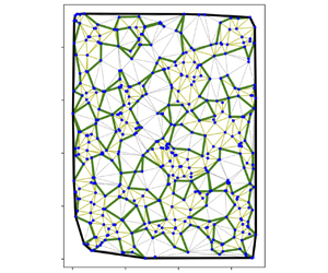
  $\alpha$-shapes for two typical particle centre-of-mass arrangements in the plateau region at the highest Reynolds numbers explored. Large holes having sizes ranging from 5 to a little more than 20 $a \phi ^{-1/3}$ are clearly displayed. These holes are somewhat larger, more numerous and more complex than those observed in the Stokes regime (Bergougnoux & Guazzelli Reference Bergougnoux and Guazzelli2009). This is shown in figure 9(c,d) by comparing two typical particle arrangements in the Stokes and weak-inertia regimes for a similar total number of particles in the plateau region.

Figure 9. Particle centre-of-mass positions (red for particles of batch  $A$ and blue for particles of batch $B$) and holes found by the approach of $\alpha$-shapes (delimited by green solid lines) for (a) particles of batch $A$ at $Re_L=24.08$ ( $Re_a=3.6\times 10^{-2}$), (b) particles of batch $B$ at $Re_L=4.20$ ( $Re_a=1.6\times 10^{-2}$), (c) particles of batch $A$ at $Re_L=0.01$ ( $Re_a=2.2\times 10^{-5}$) and (d) particles of batch $A$ at $Re_L=2.62$ ( $Re_a=3.9\times 10^{-3}$), in the plateau region. Delaunay triangulation is represented by black dotted lines inside the holes and by yellow solid lines outside the holes. The convex hull of the centre-of-mass positions corresponds to the black solid curve. Distance is plotted in mean interparticle spacings, $a \phi ^{-1/3}$.
Table 2. Exponent,  $n$, as well as mean and ( $\pm$) standard deviation of the Pearson mode, $P_1$, and median, $P_2$, skewnesses averaged in the plateau region for batches $A$ and $B$.
$B$.

4. Comparison and concluding remarks
We have examined dilute ( $\phi = 0.3\,\%$) sedimenting suspensions in large containers (larger than $20$ mean interparticle separations) when inertia is progressively increased. In these experiments, whereas the particle Reynolds number remains smaller than one ( $2 \times 10^{-5} \lesssim Re_a \lesssim 4 \times 10^{-2}$), the container Reynolds number can become greater than one ( $0.01\lesssim Re_L \lesssim 25$). The velocity fluctuations fields present the same qualitative structure as that observed in the Stokes regime across the range of Reynolds numbers explored. Initially, large-scale fluctuations dominate the dynamics. But these initial large fluctuations are transient and decay in time to weaker smaller-scale fluctuations. The smaller-scale fluctuations are then dominant in a steady plateau regime until the arrival of the upper sedimentation front. The size of these plateau fluctuations does not vary significantly with inertia in the range of Reynolds numbers explored and the long-time plateau correlation lengths in the vertical and horizontal directions are seen to be $\ell ^{\parallel }_\infty \approx \ell ^{\perp }_\infty \approx 20\text {--}30$ mean interparticle spacings. Conversely, the magnitude of the long-time plateau velocity fluctuations is seen to decrease with increasing inertia above critical Reynolds numbers $Re_a^c \approx 4 \times 10^{-4}$ and $Re_L^c \approx 0.1$, and more precisely to vary as a power $-0.1$ of the Reynolds numbers, i.e. ${\sim } Re_a^{-0.1}$ and ${\sim } Re_L^{-0.1}$.
This decrease with increasing inertia differs from the theoretical prediction in  $Re_a^{-1/2}$ of Koch (Reference Koch1993). This is not surprising as the present experiments are performed at $Re_a\ll 1$ whereas the theoretical model of Koch (Reference Koch1993) addresses dilute suspensions with Oseen wake interactions and thus the case of $Re_a \sim O(1)$. What is more striking is that this decrease is weaker than the prediction in $Re_a^{-1/3}$ of Hinch (Reference Hinch1988) and Brenner (Reference Brenner1999) designed to work for $Re_a\ll 1$ as it is the case in the present experiments.
Numerical simulations also indicate a reduction in relative fluctuations with increasing inertia (Climent & Maxey Reference Climent and Maxey2003; Yin & Koch Reference Yin and Koch2008; Sungkorn & Derksen Reference Sungkorn and Derksen2012; Hamid et al. Reference Hamid, Molina and Yamamoto2014). However, the onset of the inertial effects occurs at a particle Reynolds number much higher ( $Re_a^c\approx 0.1$) in the simulations than that found in the present experiments ( $Re_a^c \approx 4 \times 10^{-4}$), see e.g. the simulations of Yin & Koch (Reference Yin and Koch2008) and Sungkorn & Derksen (Reference Sungkorn and Derksen2012) for $\phi = 1\,\%$ and $= 0.5\,\%$ similar to the present experimental $\phi = 0.3\,\%$. The decrease in fluctuations computed in the numerical simulations is also stronger than in the present experiments. The simulations of Yin & Koch (Reference Yin and Koch2008) in cubic periodic domains find a decrease in $Re_a^{-1/2}$, in agreement with the theory of Koch (Reference Koch1993) above a region of cross-over, $0.1 < Re_a < 5$, between low- and finite- $Re_a$ behaviours. The large-box simulations of Sungkorn & Derksen (Reference Sungkorn and Derksen2012) suggest instead a decrease in $Re_a^{-0.69}$ but for $0.1\lesssim Re_a \lesssim 3$. The correlation lengths of the velocity fluctuations are also seen to decrease with increasing inertia but for $Re_a \gtrsim 0.1$ (Climent & Maxey Reference Climent and Maxey2003; Sungkorn & Derksen Reference Sungkorn and Derksen2012). Overall, most of these simulations examined the regime $Re_a \sim O(0.1\text {--}1)$ and higher wherein the inertial hydrodynamic interactions between particles may dominate. This is an inertial regime differing from that explored in the present experiments for which $Re_a \ll 1$ but $Re_L \sim O(1)$. Also, a potential issue is the use of periodic boundary conditions which somehow implies re-injecting the fluctuations from the bottom to the top of the simulation domain and may lead to an unrealistic magnitude of the fluctuations as seen in the Stokes regime (Koch Reference Koch1994; Ladd Reference Ladd2002).
We now turn to the comparison with the two experimental results available in the literature which were performed in a more confined geometry. The present findings disagree with those of Cowan et al. (Reference Cowan, Page and Weitz2000) who found no influence of inertia for  $Re_a < 1$ in a fluidised bed. But these experiments were performed at large $\phi = 20\,\%\text{--}50\,\%$ and, as mentioned in § 1, the flow of particles in a fluidised bed differs from that of sedimenting particles in a quiescent fluid. The findings of Segrè (Reference Segrè2001, Reference Segrè2007) for a sedimenting suspension of spheres quantitatively differ from the present experimental results as the onset of inertial influence is found at a higher critical $Re_a$ ( ${\sim }0.05$ for a suspension of initial volume fraction $\phi = 6\,\%$). But, as mentioned in § 1, using particle image velocimetry without index matching at such a (not so dilute) concentration is doubtful and may lead to inaccurate measurements. This may explain the disagreement. However, the idea developed that inertia onset would occur when the inertial screening length, $a/Re_a$, becomes as small as the ultimate velocity correlation length, $\ell _{\infty }$, seems reasonable. This translates to a criterion on the value of the Reynolds number, $Re_{\ell _{\infty }}=Re_a \ell _{\infty }/a$ and on the size of the ultimate correlation length (i.e. the ultimate size of the density fluctuation blob). But inertial effects are likely to happen as early as $Re^c_{\ell _{\infty }}\sim 0.1$ instead of ${\sim }1$, as observed for the drag on a sphere (Maxworthy Reference Maxworthy1965; Kumagai & Fujiwara Reference Kumagai and Fujiwara1983).
At that stage of the discussion, it is tempting to follow this latter idea from Segrè (Reference Segrè2001, Reference Segrè2007) and to extend the Caflisch–Luke–Hinch scaling to a drag experienced by the blobs which accounts for small inertial corrections instead of the large inertial forces considered by Hinch (Reference Hinch1988) and Brenner (Reference Brenner1999). In other words, the idea is to develop the argument in the intermediate region between Stokes drag and Newton drag. Using then a transitional drag  $6 {\rm \pi}\mu l w^{\prime } \mathcal {F}(Re_l)$ to balance the buoyancy force acting on the blob of size $l$ leads to $w^{\prime } (l) \sim [V_S/\mathcal {F}(Re_l)] \sqrt {\phi l/a}$ where $\mathcal {F}(Re_l)$ is the small-inertia expansion given for instance by the formula of Oseen (Reference Oseen1913), $\mathcal {F}(Re_l)=1+3Re_l /4$, or the empirical correlation of Schiller & Naumann (Reference Schiller and Naumann1933), $\mathcal {F}(Re_l)=1+0.15 Re_l^{0.687}$, with $Re_l=Re_a l/a$ (note that here $l$ corresponds to the diameter of the blob and not its radius). As in the original argument meant for the Stokes regime, the fluctuations of largest size should dominate the initial dynamics, which is indeed seen in the present experiments. But again, the large initial fluctuations decay to smaller-scale fluctuations which stay constant in a steady plateau regime. The extension of the blob model to small inertial correction is tested against the experimental data in this steady plateau regime in figure 10 by taking $l= \ell _{\infty } \approx \ell ^{\parallel }_\infty \approx \ell ^{\perp }_\infty \approx 30 a \phi ^{-1/3}$ as found experimentally in § 3.1. A decent agreement is found using the correlation of Schiller & Naumann (Reference Schiller and Naumann1933) with a constant ultimate blob size of $30 a \phi ^{-1/3}$. The onset of inertia is also correctly given by $Re^c_{\ell _{\infty }}\sim 0.1$ leading to $Re_a^c \sim 5 \times 10^{-4}$. The reduction of the fluctuations can thus be interpreted as due to the small inertial increase of the drag on the density fluctuation blob.

Figure 10. Same as figure 6(a) but with a comparison with the Caflisch–Luke–Hinch model extended to a drag experienced by the density fluctuation blobs which accounts for small inertial corrections: Schiller–Naumann (black solid curve) and Oseen (black dashed-dotted curve) corrections. The yellow dotted vertical line indicates the onset of inertial effects given by  $Re_l^c= Re_a^c 30 \phi ^{-1/3} \sim 0.1$, i.e. $Re_a^c \sim 5 \times 10^{-4}$.
However, the model underlying assumption of a random particle density distribution does not hold when inertia is increased. While, in the Stokes regime, the microstructure is not a random positioning but is still not too far from it, it becomes even more sub-homogeneous in the weak-inertia regime with many regions depopulated of particles and a few more concentrated regions. Anisotropy in the microstructure has been observed in numerical simulations and related to the wake interactions between particles in the regime  $Re_a \sim O(0.1\text {--}1)$ (see e.g. Yin & Koch Reference Yin and Koch2007; Hamid et al. Reference Hamid, Molina and Yamamoto2014). Clustering of particles has been also observed but for larger $Re_a \sim O(200)$ (Zaidi et al. Reference Zaidi, Tsuji and Tanaka2014). It would be of interest to undertake further investigations in the present regime for which $Re_a \ll 1$ but $Re_L \sim O(1)$ and to examine the interactions of the fluctuating density blobs when inertia becomes finite. An important point to understand is how a small amount of inertia leads to the growth of holes in the microstructure. One possible physical mechanism may be that centrifugal forces eject the heavy particles from the fluctuation vortices. This process is seen for particles settling in random or turbulent flows and known as preferential sweeping wherein particles preferentially sample low vorticity regions of the fluid velocity field along the gravity direction as they are centrifuged out of regions of strong vorticity (see e.g. Maxey Reference Maxey1987; Wang & Maxey Reference Wang and Maxey1993). This is also reminiscent of a scenario proposed by Batchelor & Nitsche (Reference Batchelor and Nitsche1994) discussing particles expelled by centrifugal forces from buoyant blobs leading to bubbles in fluidised beds.
Declaration of interests
The authors report no conflict of interest.


