2. Methodology

The numerical simulation of incompressible turbulent flow in non-circular ducts is a more challenging task for numerical algorithms than the canonical cases of plane channel and pipe flow. The main reason resides in the availability of only one direction of space homogeneity, which prevents the use of efficient inversion procedures for Poisson equations based on double trigonometric expansions (Kim & Moin Reference Kim and Moin1985; Orlandi Reference Orlandi2012). This difficulty has been tackled using two-dimensional Poisson solvers based on cyclic reduction (Gavrilakis Reference Gavrilakis1992), using algebraic multigrid methods (Vinuesa et al. Reference Vinuesa, Noorani, Lozano-Durán, Khoury, Schlatter, Fischer and Nagib2014; Marin et al. Reference Marin, Vinuesa, Obabko and Schlatter2016), or fast diagonalization (Pinelli et al. Reference Pinelli, Uhlmann, Sekimoto and Kawahara2010), resulting in a larger computational cost than for channel and pipe flow simulations. In the present work, we use a fourth-order co-located finite-difference solver, previously used for DNS of compressible turbulence, also in the low-Mach-number regime (Pirozzoli & Bernardini Reference Pirozzoli and Bernardini2013; Modesti & Pirozzoli Reference Modesti and Pirozzoli2016; Bernardini et al. Reference Bernardini, Modesti, Salvadore and Pirozzoli2021). Here, the convective terms in the Navier–Stokes equations are expanded preliminarily to quasi-skew-symmetric form, in such a way as to preserve discretely total kinetic energy from convection (Pirozzoli Reference Pirozzoli2010). Semi-implicit time stepping is used for time advancement in order to relax the acoustic time step limitation, thus allowing efficient operation at low Mach number, also through the use of the entropy evolution equation rather than the total energy equation (Modesti & Pirozzoli Reference Modesti and Pirozzoli2018). The streamwise momentum equation is forced in such a way as to maintain a constant mass flow rate (the spatially uniform driving term is hereafter referred to as ${\varPi }$), periodicity is exploited in the streamwise direction, and isothermal no-slip boundary conditions are used at the channel walls. Let $h$ be the duct half-side; the DNS have been carried out for a duct with $[-h:h] \times [-h:h]$ cross-section, and length $6 {\rm \pi}h$.

Six DNS have been carried out at bulk Mach number $M_b=u_b/c_w=0.2$ (where $c_w$ is the speed of sound at the wall temperature) and bulk Reynolds number ${{Re}}_b=4400\text {--}84\,000$ (table 1), and hereafter these are labelled with letters from A to F. In order to quantify the effect of secondary flows we have also carried out simulations at the same bulk Reynolds numbers, wherein secondary flows are suppressed numerically, and which are denoted with the suffix 0. The turbulence Mach number $M_t=u'/{c_w}$ nowhere exceeds $0.01$ for any of the simulations, hence the present DNS may be regarded as representative of genuinely incompressible turbulence. Issues related to the size of the computational box, mesh resolution and statistical convergence were discussed in a previous publication (Pirozzoli et al. Reference Pirozzoli, Modesti, Orlandi and Grasso2018), which focused on the analysis of the velocity statistics. In the present study, the Navier–Stokes equations are augmented with the transport equation for a passive scalar field, with molecular diffusivity $\alpha = \nu$, in such a way that the molecular Prandtl number is unity for all simulations. Although the study of passive scalars may be relevant in several fluid dynamics applications, from now on we will always refer to the transported scalar as representative of the temperature field, and the associated fluxes as representative of heat fluxes. Similarly to the streamwise velocity field, the passive scalar equation is also forced with a time-varying, spatially homogeneous forcing term (say $Q$), in such a way that its mean value is maintained in time (Pirozzoli, Bernardini & Orlandi Reference Pirozzoli, Bernardini and Orlandi2016). This forcing method corresponds to adding uniform bulk heating to balance heat losses, although other forcing strategies are possible (e.g. Piller Reference Piller2005; Abe & Antonia Reference Abe and Antonia2017). The most common alternative to uniform bulk heating is enforcement of constant heat flux in time. Both approaches have advantages and disadvantages. Uniform bulk heating is less realistic as it is difficult to attain in experiments (Piller Reference Piller2005); however, it is more efficient from a computational point of view because of faster convergence towards a statistically stationary state. In the present work, we opt for uniform bulk heating in light of higher computational efficiency in DNS of high-Reynolds-number flows. We expect that this approach may yield a slightly higher heat flux number as compared to the case of strictly constant heat flux (Abe & Antonia Reference Abe and Antonia2017; Alcántara-Ávila, Hoyas & Pérez-Quiles Reference Alcántara-Ávila, Hoyas and Pérez-Quiles2021). In the following, we use a different notation for the mean temperature in the duct,

(2.1)\begin{equation} \theta_b = \frac 1{A_c} \int_{A_c} (\varTheta-\theta_w)\,\mbox{d} A_c , \end{equation}

and for the bulk temperature,

(2.2a,b) \begin{equation} \theta_m = \frac{1}{u_b A_c} \int_{A_c} U (\varTheta-\theta_w)\,\mbox{d} A_c, \quad u_b = \frac{ 1}{A_c} \int_{A_c} U\,\mbox{d} A_c, \end{equation}

where $\theta _w$ is the wall temperature, and $A_c$ is the cross-sectional area of the duct. We use capital letters to denote flow properties averaged in the homogeneous spatial directions and in time, angle brackets to denote the averaging operator, and lower-case letters to denote fluctuations from the mean. We also exploit geometrical symmetries, and average the flow statistics over the duct quadrant or duct octant, whenever possible. The effect of quadrant averaging was discussed in detail in our previous publication Pirozzoli et al. (Reference Pirozzoli, Modesti, Orlandi and Grasso2018).

Table 1.

Flow parameters for square duct DNS. Box dimensions are $6{\rm \pi} h \times 2h \times 2h$ for all flow cases. Flow cases denoted with the 0 suffix are carried out by suppressing the secondary motions. We denote by ${{Re}}_b = 2 h u_b / \nu$ the bulk Reynolds number, and by ${{Re}}_{\tau }^* = h u_{\tau }^* / \nu$ the friction Reynolds number; $C_f = 2 \tau _w /(\rho u_b^2)$ is the friction coefficient, and ${{Nu}}$ is the Nusselt number; $\Delta x$ is the mesh spacing in the streamwise direction, and $\Delta z$, $\Delta y_w$ are the maximum and minimum mesh spacings in the cross-stream direction, all given in global wall units $\delta _v^*=\nu /u_{\tau }^*$.

The $+$ superscript is here used to denote local wall units, namely quantities made non-dimensional with respect to the local friction velocity $u_{\tau } = (\tau _w/\rho )^{1/2}$ (where $\tau _w= \rho \nu \,{\mbox {d} U}/{\mbox {d} y}\vert _w$ is the local wall shear stress), and the local viscous length scale $\delta _v=\nu /u_{\tau }$. The $*$ superscript is reserved to denote global wall units, with friction velocity based on the perimeter-averaged wall shear stress,

(2.3)\begin{equation} u^*_{\tau} = \left( \frac {\tau^*_w}{\rho} \right)^{1/2} = \left( \frac { h \left\langle \varPi \right\rangle }{2 \rho} \right)^{1/2}, \end{equation}

and viscous length scale $\delta _v^*=\nu /u_{\tau }^*$. Likewise, for normalization of the temperature field, we consider either the local friction temperature,

(2.4)\begin{equation} \theta_{\tau} = \frac {q_w}{u_{\tau}}, \end{equation}

where $q_w = \alpha \,{\mbox {d} {\varTheta }}/{\mbox {d} y}\vert _w$ is the local wall heat flux, or the global friction temperature,

(2.5)\begin{equation} \theta^*_{\tau} = \frac {q^*_w}{u^*_{\tau}} = \frac{ \left\langle {Q} \right\rangle h}{2 u^*_{\tau}}. \end{equation}

Equations (2.3) and (2.5) make it clear that the global friction velocity and temperature are related to the imposed forcing of the streamwise momentum and temperature equations, rather than to the detailed distribution of wall momentum and temperature fluxes. Notably, local and global wall units collapse in the case of canonical wall-bounded flows because of homogeneity, but the two are distinctly different in internal flows in non-circular ducts. DNS studies such as the present one can then be used to distinguish between the two scalings, which is impossible in more canonical set-ups.

3. Temperature statistics

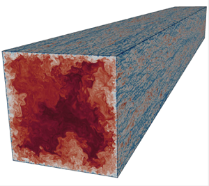
We begin by inspecting the instantaneous streamwise velocity and temperature fields in figure 1, which shows the flow in both the cross-stream and wall-parallel planes. The instantaneous flow structures are not different from those typical of canonical wall-bounded flows, and the near-wall region is populated with temperature and streamwise velocity streaks, resulting from sweep and ejections events visible in the cross-stream plane. Large structures are also visible in the cross-stream plane, which convey high-speed, hot flow from the duct core towards the corners, and which interact with the smaller near-wall flow structures. Return motions of low-speed, cool fluid are also observed to emerge from around the bisector of each side of the square duct. These observations suggest that the secondary motions resulting from space- and time-averaging are not just an artefact, but they are well present in the instantaneous flow realizations. Similarity between streamwise velocity and temperature is apparent, with the main difference that the latter reveals finer structures and sharper fronts owing to the absence of the smoothing action of pressure (Pirozzoli et al. Reference Pirozzoli, Bernardini and Orlandi2016).

Figure 1.

Instantaneous streamwise velocity (a) and temperature (b) fields for flow case F. Wall-parallel planes are taken at fifteen wall units from the walls.

Figure 2 depicts the mean temperature (contours) and velocity (isolines) fields in the duct cross-section, along with representative cross-stream velocity vectors. This representation brings to light the presence of a pair of counter-rotating secondary eddies in each quarter of the domain, whose apparent role is bringing high-speed and high-temperature fluid from the duct core towards the corners, to compensate for the deficit. As a result, both the temperature contours and the velocity isolines bend towards the corners, featuring a bulging first noticed by Nikuradse (Reference Nikuradse1930). This effect seems to be non-monotonic with the Reynolds number, being most evident for DNS-A and DNS-E/F. As expected, temperature and velocity contours bear close similarity, being nearly coincident near the wall, and retaining the same shape farther off. This analogy is the result of the formal similarity of the controlling equations, and it is further investigated in figure 3, where we show a scatter plot of mean velocity and temperature. In the near-wall region (say, $U^* \le 10$), perfect matching is recovered (namely, $\varTheta ^* = U^*$), which is not surprising, as at unit Prandtl number, $\varTheta ^+ \equiv U^+ \equiv y^+$ in the wall vicinity. However, near equality of the two distributions in global wall units is less trivial and is a symptom of strong similarity between the two fields. At non-unit Prandtl number, we still expect a linear relationship to be present like $\varTheta ^* = {{Pr}} \, U^*$, since in general $\varTheta ^+ \equiv U^+ \equiv {{Pr}} \, y^+$ in the wall vicinity (Kader Reference Kader1981). Farther from walls ($U^* \gtrsim 15$, which corresponds to the root of the logarithmic layer in canonical wall-bounded flows), a linear imprinting is still visible, although with larger scatter than in the near-wall region, and with slope shallower than unity. This can be explained by recalling (Pirozzoli et al. Reference Pirozzoli, Bernardini and Orlandi2016) that in canonical flows, the distributions of both velocity and temperature are nearly logarithmic, but with different slope. In particular, currently accepted values of the Kármán constant are $\kappa \approx 0.39$ for the mean velocity, and $\kappa _{\theta } \approx 0.46$ for the mean temperature. As a matter of fact, the scatter plot is well fitted with a linear function with slope $\kappa /\kappa _{\theta } \approx 0.84$. At ${{Pr}} \ne 1$, we thus expect a similar relationship, but with different additive constant, as a result of the different intercept in the log law for the temperature field. This observation is quite interesting in our opinion, as the presence of a (nearly) universal relationship between mean velocity and temperature in a non-trivial flow in a square duct in principle would allow us to reconstruct directly the whole temperature field based on the velocity field.

Figure 2.

Mean streamwise temperature (${\varTheta }^*$, flooded contours), mean streamwise velocity (${U}^*$, lines), and mean cross-stream velocity vectors ($V^*, W^*$) for flow cases A (a), B (b), C (c), D (d), E (e), F ( f). For clarity, only a subset of the velocity vectors is shown, and only a quarter of the full domain is shown. The dashed diagonal lines indicate the corner bisector.

Figure 3.

Scatter plot of mean temperature ($\varTheta ^*$) versus mean velocity ($U^*$) for DNS data of all flow cases, and corresponding fitting functions for the near-wall region, $\varTheta ^* = U^*$ (dashed line), and for the outer region, $\varTheta ^* = 2.57 + 0.84 U^*$ (solid line). Colours are as in table 1.

Based on the previous observations, it is natural to study and compare the temperature statistics expressed in local wall units ($+$) and in global wall units ($*$). Figure 4 shows the mean temperature profiles as a function of the wall-normal distance up to the corner bisector (white dashed line in figure 2), in local wall units. For reference purposes, the mean temperature profiles obtained from the experimental fitting by Kader (Reference Kader1981) at matching ${{Re}}_{\tau }$ are also reported. Excellent collapse of the locally scaled profiles is recovered near the wall, also including the near-corner region. The distributions become more widespread past $y^+ \approx 10$, with maximum scatter of about $\pm$5 % in the ‘logarithmic’ layer. When the global friction temperature is used for normalization (see figure 5), scatter among the temperature profiles is observed near the wall as a result of the local variation of the wall heat flux. Perhaps unexpectedly, this normalization does yield similarly good universality away from walls, and near coincidence with the pipe temperature profiles, at least at high enough Reynolds numbers. This finding is probably related to the fact that mean temperature transport away from solid walls is controlled by the imposed spatially uniform heat source rather than by the non-uniform wall heat flux. Inspection of figure 5 shows that transition from wall scaling to ‘global’ scaling (which is controlled by the spatially uniform heat source) occurs at a wall distance of about $0.2 h$, which is also the lower limit for the core region in canonical flows (Pope Reference Pope2000). This observation seems to support the validity of Townsend's outer layer similarity also for the temperature field, in that the outer flow perceives mainly the global heat flux and not its detailed local distribution at the wall. Validity of outer-layer similarity for the temperature field was reported for rough walls (MacDonald, Hutchins & Chung Reference MacDonald, Hutchins and Chung2019), whereas we are not aware of similar conclusions for the case of more complex geometries because most studies on forced convection are limited to canonical wall-bounded flows, in which the wall heat flux is spatially uniform. These results support findings reported previously for the streamwise velocity (Pirozzoli et al. Reference Pirozzoli, Modesti, Orlandi and Grasso2018), and confirm that square duct flow is a convenient testbed for evaluating differences between local and global scaling.

Figure 4.

Mean wall-normal temperature profiles scaled in local wall units for flow cases A (a), B (b), C (c), D (d), E (e), F ( f). Profiles are plotted at several distances from the left wall, up to the corner bisector (see figure 2 for reference): $z^*=15$ (diamonds), $z/h=0.1$ (right triangles), $z/h=0.25$ (triangles), $z/h=0.5$ (circles), $z/h=1$ (squares). The dashed lines denote fits of experimental data (Kader Reference Kader1981) at matching ${{Re}}_\tau ^*$.

Figure 5.

Mean wall-normal temperature profiles scaled in global wall units for flow cases A (a), B (b), C (c), D (d), E (e), F ( f). Profiles are plotted at several distances from the left wall, up to the corner bisector (see figure 2 for reference): $z^*=15$ (diamonds), $z/h=0.1$ (right triangles), $z/h=0.25$ (triangles), $z/h=0.5$ (circles), $z/h=1$ (squares). The dashed lines denote fits of experimental data (Kader Reference Kader1981) at matching ${{Re}}_\tau ^*$.

The fluctuating velocity and temperature fields in the vicinity of the duct corners are shown in figure 6 upon global inner normalizations, as well as the corresponding correlation coefficients. To facilitate comparison across the Reynolds number range, the horizontal coordinate is reported in inner units up to $z^*=150$, and the vertical one in outer units. This allows simultaneous visualization of both the corner and the core region, at all Reynolds numbers. Far from the corner, the distributions of the velocity and temperature variances are nearly unaffected by Reynolds number variation, and feature a buffer-layer peak at a distance of about fifteen wall units from the closer wall. The amplitude of the peak is reduced moving towards the corner, whose effect is felt to within a distance of $O(100)$ global wall units. The $u$–$\theta$ correlation coefficient shows strict similarity of velocity and temperature fluctuations also in the instantaneous sense, with the exception of the close neighbourhood of the corner. Correlation in the outer layer is less than near the wall, but it tends to increase at higher Reynolds number, similar to the case of plane channel flow (Pirozzoli et al. Reference Pirozzoli, Bernardini and Orlandi2016).

Figure 6.

Streamwise velocity and temperature fluctuation intensities (in global inner units), and their correlation coefficient, in the proximity of a duct corner for flow cases A (a–c), B (d–f), C (g–i), D (j–l), E (m–o), F (p–r). Note that the horizontal coordinate ($z$) is given in inner units, and the vertical coordinate $y$ is given in outer units and at a logarithmic scale.

A quantitative analysis of the buffer-layer peaks of the velocity and temperature variances is reported in figure 7. Specifically, for each horizontal location ($z$, measured from the corner), we show the peak variances of $u$ and $\theta$ expressed in local wall units. In this respect, we note that $z^+$ can be interpreted as effective local friction Reynolds numbers, based on the distance of the wall point from the corner bisector (see figure 2). It is known that in canonical flows (Marusic et al. Reference Marusic, Monty, Hultmark and Smits2013), the peak velocity variances increase logarithmically with the friction Reynolds number. Hence it is interesting to verify whether the same trend also occurs in flows involving non-trivial cross-sections, and featuring secondary motions. For that purpose, in both panels of figure 7 we show the logarithmic trend predicted by Marusic et al. (Reference Marusic, Monty, Hultmark and Smits2013) as benchmark. It is noteworthy that away from the corner (say $z^+ \gtrsim 100$), local wall units yield good universality of the distributions, and suggest an increasing trend of the variances with the local friction Reynolds number. However, the growth rate seems to be far less than in canonical flows, possibly violating Townsend's attached-eddy hypothesis. We speculate that this peculiar behaviour may be due to either disruption of the hierarchy of wall-attached eddies because of the action of secondary motions, or perhaps impeded spanwise growth caused by the presence of corners, both effects being absent in planar channel or pipe flow.

Figure 7.

Inner-layer peak variances of axial velocity (a), and temperature (b), expressed as functions of the local friction Reynolds number ($z^+$). The dashed lines denote the logarithmic fit for canonical flows (Marusic, Baars & Hutchins Reference Marusic, Baars and Hutchins2017), namely $\langle u^2\rangle ^+_{{IP}} = 0.63 \log {{Re}}_{\tau } + 3.8$. Symbols as in table 1.

The distributions of the local friction and heat transfer coefficients along the duct wall are shown in figure 8. As shown previously by Pirozzoli et al. (Reference Pirozzoli, Modesti, Orlandi and Grasso2018), the distribution of the wall friction coefficients is non-monotonic, featuring a peak at the side bisector, and a secondary peak near the corner, at a distance scaling with global wall units. As from theoretical predictions (Spalart, Garbaruk & Stabnikov Reference Spalart, Garbaruk and Stabnikov2018), the friction tends to equalize over the duct perimeter at higher ${{Re}}$. The heat transfer coefficient seems to have the same qualitative behaviour, thus corroborating the experimental observations of Brundrett & Burroughs (Reference Brundrett and Burroughs1967) and Hirota et al. (Reference Hirota, Fujita, Yokosawa, Nakai and Itoh1997). Quantitative assessment is shown in figure 8(c), where we show the Reynolds analogy factor $2 {{St}} / C_f$, which is expected to be unity at ${{Pr}} = 1$ (White & Majdalani Reference White and Majdalani2006). In fact, whereas deviations are observed at low Reynolds numbers, the distribution corresponding to DNS-F varies between 0.98 and 1.2, right at the corner.

Figure 8.

Distributions of local wall friction coefficient $C_f=2 u_{\tau }^2/u_b^2$ (a), local Stanton number ${{St}}=(u_{\tau } \theta _{\tau })/(u_b \theta _m)$ (b), and Reynolds analogy factor (c), along the left part of the lower wall. Symbols as in table 1.

The overall heat transfer performance of the duct is quantified in terms of the global Stanton number,

(3.1)\begin{equation} {{St}}^* = \frac{q_w^*}{u_b \theta_m} = \frac 1{u_b^* \theta_m^*}, \end{equation}

or more frequently in terms of the Nusselt number,

(3.2)\begin{equation} {{Nu}}^* = {{St}}^* \, {{Re}}_b \, {{Pr}} . \end{equation}

In figure 9, we compare the distributions of the heat transfer coefficients (inverse Stanton number and Nusselt number) obtained from the present DNS (squares) with those resulting from DNS of circular pipe flow (circles), from previous LES (diamonds), and from experiments (triangles) in square ducts. We note that the latter two datasets were obtained for ${{Pr}}=0.71$, hence the ${{Nu}}$ data are rescaled by a factor $1/\sqrt {{{Pr}}}$ to compare with the present ones. As a reference, we also report correlations used widely in engineering practice, including that from Gnielinski (Reference Gnielinski1976),

(3.3) \begin{equation} {{Nu}} = \frac{{{Pr}}\,(C_f/32) ( {{Re}}_b - 1000 )}{1 + 12.7 (C_f/32)^{1/2} ( {{Pr}}^{2/3} - 1)}, \end{equation}

and from Kays & Crawford (Reference Kays and Crawford1993),

(3.4)\begin{equation} {{Nu}} = 0.022 \, {{Re}}_b^{0.8} \, {{Pr}}^{0.5}. \end{equation}

Finally, direct fitting the present DNS data (at ${{Pr}}=1$) with a power-law expression yields

(3.5)\begin{equation} {{Nu}} = 0.0216 \, {{Re}}_b^{0.805}. \end{equation}

Figure 9.

Inverse global Stanton number (a) and Nusselt number (b) as functions of bulk Reynolds number, from the present DNS (squares), from DNS of circular pipe flow (circles, Pirozzoli et al. Reference Pirozzoli, Romero, Fatica, Verzicco and Orlandi2021), from previous LES (diamonds, Pallares & Davidson Reference Pallares and Davidson2002), and from experiments (triangles, Brundrett & Burroughs Reference Brundrett and Burroughs1967). The dashed lines denote the correlation (3.4), and the dot-dashed lines denote the correlation (3.3).

The DNS data show good correspondence with the pipe DNS data at matching ${{Re}}_b$, with the exception of the lower Reynolds number case, which supports validity of the hydraulic diameter concept as the relevant length scale for heat transfer data reduction. Agreement with experiments and LES in square ducts is also quite good, on account of experimental uncertainties and modelling errors in LES. It is interesting that differences are levelled off when the popular representation in terms of the Nusselt number is used, as in figure 9(b), hence we believe that the $1/{{St}}$ representation should be used when relatively small differences must be discriminated. Classical correlations seem to suggest systematic difference of up to $5\,\%$ in the prediction of the heat transfer coefficient. This difference may be due partly to inaccuracy of correlations based on old experimental data, or to the fact that those are trained mainly for the ${{Pr}}=0.71$ case, whereas here ${{Pr}}=1$. Discrepancies can also be attributed partly to our heat forcing scheme, in which a spatially uniform heat source is prescribed, which tends to slightly overpredict the heat flux as compared to other approaches in which the total heat flux is maintained strictly constant in time (Abe & Antonia Reference Abe and Antonia2017; Alcántara-Ávila et al. Reference Alcántara-Ávila, Hoyas and Pérez-Quiles2021). A slight adjustment of the Kays–Crawford power-law formula coefficients as after (3.5) seems to yield very good representation of the DNS data.

An issue that deserves further investigation is why use of the hydraulic diameter yields excellent results, at least in the case of square ducts under consideration. Pirozzoli et al. (Reference Pirozzoli, Modesti, Orlandi and Grasso2018) showed that universality of friction is connected with near applicability of the logarithmic velocity law in the direction normal to the nearest wall. It is worthwhile verifying whether this is also the case for the heat flux coefficient. As shown previously, the temperature distributions are nearly universal away from walls, even when expressed in global wall units. Hence, approximating the outer layer profiles with the classical log law, namely $U^*=1/{\kappa } \log y^* + C$, $\varTheta ^*=1/\kappa _{\theta } \log y^* + C_{\theta }$, and integrating over the duct cross-section, gives the following expression for the inverse Stanton number velocity:

(3.6)\begin{align} 1 / {{St}}^* &= u_b^* \theta_m^* = \frac{8}{4{{Re}}_\tau^{*2}} \int_0^h\int_0^z\left[\frac{1}{\kappa \kappa_\theta}\log{y^*}^2 + \log{y^*} \left(\frac{C_\theta}{\kappa} + \frac{C}{\kappa_\theta}\right) +CC_\theta\right]{{\rm d}y}^*\,{\rm d} z^* \nonumber\\ &=\frac{1}{\kappa \kappa_\theta}\left(\log^2{{{Re}}_\tau^*} + 3\log{{{Re}}_\tau^*} + \frac{7}{2}\right) + \left(\frac{C_\theta}{\kappa}+\frac{C}{\kappa_\theta}\right) \left(\log{{{Re}}_\tau^*}-\frac{3}{2}\right) + CC_\theta. \end{align}

Equation (3.6) should be compared with the corresponding expression for a circular duct with diameter $D$,

(3.7)\begin{equation} 1 / {{St}} = \frac{1}{\kappa \kappa_\theta}\left(\log^2{{{Re}}_\tau} + 3\log{{{Re}}_\tau} + \frac{7}{2}\right) + \left(\frac{C_\theta}{\kappa}+\frac{C}{\kappa_\theta}\right) \left(\log{{{Re}}_\tau}-\frac{3}{2}\right) + CC_\theta, \end{equation}

where ${{Re}}_{\tau } = D u_{\tau } / (2 \nu )$. The two expressions are identical for $2 h = D$, hence the Reynolds number based on the hydraulic diameter is the same. It is interesting that (3.6) is arrived at basically by neglecting the local wall shear stress and heat flux variation along the duct perimeter, and disregarding the flow deceleration at corners. Apparently, these effects very nearly cancel out upon integration.

4. Contribution of secondary flows to heat transfer

In order to quantify the effects of secondary motions on heat transfer, we derive a generalized version of the Fukagata–Iwamoto–Kasagi (FIK) identity (Fukagata, Iwamoto & Kasagi Reference Fukagata, Iwamoto and Kasagi2002) for the Stanton number, by following the approach of Modesti et al. (Reference Modesti, Pirozzoli, Orlandi and Grasso2018). We consider the mean temperature balance equation,

(4.1)\begin{equation} \alpha \nabla^2 \varTheta = \boldsymbol{\nabla} \boldsymbol{\cdot}\boldsymbol{q}_C + \boldsymbol{\nabla}\boldsymbol{\cdot}\boldsymbol{q}_T - \langle{Q}\rangle, \end{equation}

where $\boldsymbol {q}_C={\varTheta }\,{\boldsymbol {U}}_{yz}$ is associated with mean cross-stream convection (hence, with the secondary motions), $\boldsymbol {q}_T={\langle \theta \boldsymbol {u}_{yz} \rangle }$ is associated with turbulence convection, $\boldsymbol {u}_{yz}=({v},{w})$ is the cross-stream velocity vector, and $\langle {Q}\rangle$ is the mean driving bulk heating.

Equation (4.1) may be interpreted as a Poisson equation for the mean temperature, with source terms $\boldsymbol {\nabla }\boldsymbol {\cdot }\boldsymbol {q}_T$, $\boldsymbol {\nabla }\boldsymbol {\cdot }\boldsymbol {q}_C$ and $\langle Q\rangle$ obtained from the DNS dataset. Hence the solution of (4.1) may be cast formally as the superposition of three parts, namely ${\varTheta }={\varTheta }_D+{\varTheta }_T+{\varTheta }_C$, and these temperature fields can be obtained by solving three Poisson equations,

(4.2a–c)\begin{equation} \alpha \nabla^2{\varTheta}_D={-}\langle{Q}\rangle,\quad \alpha \nabla^2{\varTheta}_T=\boldsymbol{\nabla}\boldsymbol{\cdot}\boldsymbol{q}_T,\quad \alpha \nabla^2{\varTheta}_C=\boldsymbol{\nabla}\boldsymbol{\cdot}\boldsymbol{q}_C, \end{equation}

with homogeneous boundary conditions, where ${\varTheta }_D$, ${\varTheta }_T$ and ${\varTheta }_C$ denote the diffusion, turbulence and convection contributions to the mean temperature field. Accordingly, the mean temperature in the duct may be evaluated as

(4.3a,b)\begin{equation} \theta_b=\frac {\langle{Q}\rangle A}{\alpha}\,{\theta_b}_1+{\theta_b}_T+{\theta_b}_C, \quad {\theta_b}_X = \frac{1}{A} \int_A {\varTheta}_X\,\mathrm{d}A, \end{equation}

where we have introduced the unitary Stokes temperature field $\theta _1$, defined as the solution of $\nabla ^2 \theta _1 = -1/A$, which by construction is a function of only the duct geometry, and which allows us to express the diffusion-associated temperature field as $\varTheta _D= A \, \theta _1 \langle {Q}\rangle / \alpha$. For convenience, in the present analysis we use a modified form of the Stanton number, based on the mean temperature rather than on the bulk temperature, namely

(4.4)\begin{equation} {{St}}_b^* = \frac{q_w^*}{u_b \theta_b}= \frac 1{u_b^* \theta_b^*}, \end{equation}

instead of (3.1), which when substituted into (4.3a,b) yields

(4.5)\begin{equation} {{St}}_b^* = \frac{1}{{{Pr}}\,{{Re}}_P\,{\theta_b}_1}\left(1-\frac{{\theta_b}_T}{\theta_b} - \frac{{\theta_b}_C}{\theta_b} \right)={{St}}_D + {{St}}_T + {{St}}_C, \end{equation}

where ${{Re}}_P=u_b P / \nu$ is the bulk Reynolds number based on the duct perimeter $P$. Equation (4.5) shows clearly that the heat transfer coefficient may be regarded as the sum of contributions due to diffusion, turbulence and convection (labelled as ${St}_X$ in (4.5)), and it yields an expression similar to that from the classical FIK identity for the friction coefficient.

We note that this formalism has additional generality compared to the classical FIK identity and its extensions (Peet & Sagaut Reference Peet and Sagaut2009; Jelly, Jung & Zaki Reference Jelly, Jung and Zaki2014), and it allows us to isolate the effects of mean convection, turbulence and diffusion terms to the wall shear stress distributions along the duct perimeter, resulting from

(4.6a–c)\begin{equation} {q_w}_D = \alpha \left.\frac{\partial {\varTheta}_D}{\partial y}\right\rvert_w, \quad {q_w}_T = \alpha \left.\frac{\partial {\varTheta}_T}{\partial y}\right\rvert_w, \quad {q_w}_C = \alpha \left.\frac{\partial {\varTheta}_C}{\partial y}\right\rvert_w. \end{equation}

Regarding (4.6a–c), it is important to note that only ${q_w}_D$ has non-zero mean, whereas integration of (4.2a–c) for ${\varTheta }_C$ and ${\varTheta }_T$ shows readily that their integrated contributions vanish, as $\boldsymbol {q}_C$ and $\boldsymbol {q}_T$ are both zero at walls. The contributions to the mean heat transfer coefficients are given in table 2, both in absolute terms and as a fraction of the total. Consistent with physical expectations, the diffusion contribution is observed to decline at increasing Reynolds number with respect to the turbulent term. The contribution of cross-stream convection is found to be roughly constant across the explored Reynolds number range; however, it remains much less than the turbulence contribution. Extrapolating the DNS data, we expect the convection contribution to exceed the diffusion one at high enough Reynolds number. Figure 10 shows the mean temperature fields associated with the diffusion, turbulence and convection terms. For the sake of clarity, each contribution is normalized with the corresponding bulk value, ${\theta _b}_X$, where ${\theta _b}_T$ and ${\theta _b}_C$ are both negative, thus providing an additive effect to the heat transfer (see (4.5)). The diffusion-associated temperature field $\varTheta _V$ arises from the solution of a Poisson equation with uniform right-hand side (the heat source), hence its shape is identical to the case of laminar flow (Shah & London Reference Shah and London2014), depending only on the duct cross-sectional geometry. The turbulence-associated temperature field $\varTheta _T$ is everywhere negative and topologically similar to the diffusion-associated field, highlighting the cooling effect of turbulence on the bulk flow, with incurred increase of the heat transfer coefficient. The temperature field $\varTheta _C$ associated with mean convection has a more complex organization. Positive values are found near the duct corners, whereas negative values are found near the duct bisectors, the zero crossings being located halfway in between. This finding is consistent with the intuitive expectation that secondary motions tend to equalize temperature across the duct cross-section, thus quantitatively corroborating claims made by early investigators (Prandtl Reference Prandtl1927). Notably, all the distributions shown in figure 10 are not qualitatively affected by Reynolds number variation when scaled with respect to their mean integral value, thus showing that changing the Reynolds number changes only the relative importance of the three terms, as quantified in table 2.

Figure 10.

Contributions of diffusion, turbulence and mean convection terms to the mean temperature field, as determined by solving (4.2a–c), for flow cases A (a–c), B (d–f), C (g–i), D (j–l), E (m–o), F (p–r).

Table 2.

Contributions of diffusion, turbulence and mean convection terms to the heat transfer coefficient, as from (4.5).

The observations made regarding the organization of the temperature field have a direct impact on the distribution of the local wall heat flux, shown in figure 11. The heat flux distribution induced by diffusion terms is the same for all cases, and nearly parabolic in shape. The turbulence terms have a complex behaviour, exhibiting multiple peaks that change with the Reynolds number. In general, they yield heat flux increase toward the duct bisectors, and slight attenuation at the corners (compare the lines with circles and with dots), thus making the heat flux distributions more non-uniform. Mean convection yields large positive peaks in the corner vicinity, whose distance from the neighbouring walls scales in inner units (Pirozzoli et al. Reference Pirozzoli, Modesti, Orlandi and Grasso2018), and negative values around the duct bisector. As a result, the distributions of the heat flux tend to be rather flat, especially at higher Reynolds numbers.

Figure 11.

Contributions to mean wall heat flux (shown along half a duct side) for flow cases A (a), B (b), C (c), D (d), E (e), F ( f): diffusive (${q_w}_D(z)$, dotted), turbulent (${q_w}_T(z)$, dashed), diffusive + turbulent (${q_w}_D(z)+{q_w}_T(z)$, circles), mean convection (${q_w}_C(z)$, dash-dotted), and total ($q_w(z)$, solid line).

As an alternative to quantify the effect of secondary flows we have also considered the approach of Modesti et al. (Reference Modesti, Pirozzoli, Orlandi and Grasso2018), and carried out numerical experiments at the same bulk Reynolds numbers as the baseline cases, whereby the secondary motions are suppressed artificially (flow cases with the 0 suffix in table 1). For that purpose, we force the streamwise-averaged cross-stream velocity components to have zero mean by setting

(4.7a)$$\begin{gather} v(x,y,z,t) \rightarrow v(x,y,z,t) - \overline{v}^x(y,z,t), \end{gather}$$

(4.7b)$$\begin{gather}w(x,y,z,t) \rightarrow w(x,y,z,t) - \overline{w}^x(y,z,t), \end{gather}$$

at each Runge–Kutta sub-step, where $\overline {(.)}^x$ denotes the streamwise averaging operator. Figure 12 shows the temperature contours with superimposed streamwise velocity isolines for flow cases A0–D0. We note that the typical bulging of velocity and temperature towards the corners is absent for these cases, and the core region shows near axial symmetry as in circular pipe flow. The mean velocity and temperature fields are nearly coincident at low Reynolds numbers, whereas differences become more evident as ${{Re}}_b$ increases. Although the mean flow fields in figure 12 obviously differ from the full DNS cases shown in figure 2, the heat transfer is found to be barely affected. In fact, similar to what is reported by Modesti et al. (Reference Modesti, Pirozzoli, Orlandi and Grasso2018) for frictional drag, suppressing the secondary flows yields even higher heat transfer at low Reynolds numbers, whereas a bare $3\,\%$ decrease of the Nusselt number is found for flow case $D0$; see table 1. These figures are consistent with those suggested by the FIK identity, which actually returns about $3\,\%$ contribution of secondary flows to global heat transfer for flow case D.

Figure 12.

Flow cases without secondary motions: mean streamwise velocity (${U}^*$, lines), and mean temperature (${\varTheta }^*$, flooded contours), for flow cases A0 (a), B0 (b), C0 (c), D0 (d). Only a quarter of the full domain is shown. The dashed diagonal lines indicate the corner bisector.

5. Modelling the turbulent heat flux

The numerical solution of the Reynolds-averaged Navier–Stokes equations is a common approach for flows of industrial interest. Solution of the temperature field requires a suitable closure model for the turbulent heat flux vector, $\boldsymbol {q}=\langle {\boldsymbol {u}\theta }\rangle$. Such closures are typically less sophisticated than those developed for momentum flux, and generally rely on validity of the Reynolds analogy. The primary outcome of this school of thought is the popularity retained over the years by the turbulent Prandtl number,

(5.1)\begin{equation} {{Pr}}_t=\frac{\nu_t}{\alpha_t}, \end{equation}

where $\nu _t$ and $\alpha _t$ are the eddy viscosity and eddy diffusivity coefficients, respectively. These coefficients are the heart of the linear eddy-viscosity hypothesis and its heat transfer counterpart,

(5.2a,b)\begin{equation} \tilde{\boldsymbol{a}} ={-}\nu_t \left( \boldsymbol{\nabla} \boldsymbol{U} + \boldsymbol{\nabla} \boldsymbol{U}^{\rm T} \right), \quad \tilde{\boldsymbol{q}} ={-}\alpha_t \boldsymbol{\nabla} \varTheta, \end{equation}

where $\tilde {\boldsymbol {a}}$ is the modelled counterpart of the anisotropic Reynolds stress tensor ($\boldsymbol {a}=\boldsymbol {\tau }-2/3 k$), and $\tilde {\boldsymbol {q}}$ is the modelled turbulent heat flux vector, with $\boldsymbol {\tau }=\langle {\boldsymbol u \boldsymbol u}\rangle$ and $k=1/2 \, \mathrm {tr} (\boldsymbol {\tau })$. Most heat transfer models assume a uniform turbulent Prandtl number (${{Pr}}_t \approx 1$) to avoid solving ad hoc transport equations for $\alpha _t$, although this hypothesis is not always accurate (Pirozzoli et al. Reference Pirozzoli, Bernardini and Orlandi2016; Kaller et al. Reference Kaller, Pasquariello, Hickel and Adams2019). Even assuming that the approximation ${{Pr}}_t \approx 1$ holds, limitations of the linear eddy-viscosity hypothesis (5.2a,b) are evident, and reliance on the turbulent Prandtl number concept replicates modelling inaccuracies. Pope (Reference Pope1975) extended the eddy-viscosity ansatz by using a tensor polynomial to model $\tilde {\boldsymbol {a}}$. This approach is mathematically sound because it relies on the Cayley–Hamilton theorem. In fact, it turns out that five tensor bases are in most cases sufficient to recover an exact representation of $\tilde {\boldsymbol {a}}$ (Gatski & Speziale Reference Gatski and Speziale1993; Jongen & Gatski Reference Jongen and Gatski1998; Modesti Reference Modesti2020). The same mathematical framework was extended to scalar flux modelling, both for heat transfer (So, Jin & Gatski Reference So, Jin and Gatski2004a; Younis, Speziale & Clark Reference Younis, Speziale and Clark2005; Wang et al. Reference Wang, Yee, Yin and Bergstrom2007) and for buoyancy (So, Jin & Gatski Reference So, Jin and Gatski2004b). Similar to the original tensor polynomial expansion of Pope (Reference Pope1975), the turbulent heat flux is expanded as

(5.3)\begin{equation} \tilde{\boldsymbol{q}} = \sum_{n=1}^{N}\alpha^{(n)}\boldsymbol{V}^{(n)},\quad N=1, \ldots, 10, \end{equation}

where the coefficients $\alpha ^{(n)}$ are scalar functions, and $\boldsymbol {V}^{(n)}$ is a set of ten vector bases,

(5.4) \begin{equation} \left.\begin{array}{lll@{}} &\boldsymbol{V}^{(1)}= \boldsymbol\nabla\varTheta, &\qquad\quad \boldsymbol{V}^{(6)} = \boldsymbol{\varOmega}\boldsymbol\nabla\varTheta,\\ &\boldsymbol{V}^{(2)}= \boldsymbol{a}\boldsymbol\nabla\varTheta, &\qquad\quad \boldsymbol{V}^{(7)} = \boldsymbol{\varOmega}\boldsymbol{\varOmega}\boldsymbol\nabla\varTheta,\\ &\boldsymbol{V}^{(3)}= \boldsymbol{S}\boldsymbol\nabla\varTheta, &\qquad\quad \boldsymbol{V}^{(8)} = \left(\boldsymbol{S}\boldsymbol{\varOmega}+\boldsymbol{\varOmega}\boldsymbol{S}\right)\boldsymbol\nabla\varTheta,\\ &\boldsymbol{V}^{(4)}= \boldsymbol{a}\boldsymbol{a}\boldsymbol\nabla{\varTheta}, &\qquad\quad \boldsymbol{V}^{(9)} = \left(\boldsymbol{a}\boldsymbol{S}+\boldsymbol{S}\boldsymbol{a}\right)\boldsymbol\nabla\varTheta,\\ &\boldsymbol{V}^{(5)}= \boldsymbol{S}\boldsymbol{S}\boldsymbol\nabla{\varTheta}, &\qquad\quad \boldsymbol{V}^{(10)} = \left(\boldsymbol{\varOmega}\boldsymbol{S}+\boldsymbol{S}\boldsymbol{\varOmega}\right)\boldsymbol\nabla\varTheta, \end{array}\right\} \end{equation}

where $\boldsymbol {S} = 1/2 ( \boldsymbol {\nabla } \boldsymbol {U} + \boldsymbol {\nabla } \boldsymbol {U}^\textrm {T} )$ and $\boldsymbol {\varOmega } = 1/2 ( \boldsymbol {\nabla } \boldsymbol {U} - \boldsymbol {\nabla } \boldsymbol {U}^\textrm {T} )$ are the mean strain-rate and rotation-rate tensors, respectively. As for the Reynolds stress tensor, in most practical flow cases, the ten bases are not independent, and an exact representation of the turbulent heat flux ($\tilde {\boldsymbol {q}}=\boldsymbol {q}$) is recovered for $N=3$. In order to assess the accuracy of different truncations of the polynomial expansion (5.3), we compute the coefficients $\alpha ^{(n)}$ following the approach of Jongen & Gatski (Reference Jongen and Gatski1998) and Modesti (Reference Modesti2020): namely, we take the scalar product of (5.3) with each vector basis $\boldsymbol {V}^{(m)}$, thus obtaining a linear system of $N$ equations for the unknown coefficients $\alpha ^{(n)}$:

(5.5)\begin{equation} \boldsymbol{q}\boldsymbol{\cdot}\boldsymbol{V}^{(m)} = \sum_{n=1}^{N} \alpha^{(n)}\boldsymbol{V}^{(n)}\boldsymbol{\cdot}\boldsymbol{V}^{(m)},\quad m=1,\ldots, N. \end{equation}

For $N=1$, this approach yields the standard definition of linear eddy diffusivity,

(5.6)\begin{equation} \alpha_t={-}\alpha^{(1)}={-}\frac{\boldsymbol{q}\boldsymbol{\cdot}\boldsymbol\nabla\varTheta}{\boldsymbol\nabla \varTheta\boldsymbol{\cdot}\boldsymbol\nabla\varTheta}, \end{equation}

in analogy with the definition of linear eddy viscosity,

(5.7)\begin{equation} \nu_t={-}\frac{\left\{\boldsymbol{a}\boldsymbol{S}\right\}}{2\left\{\boldsymbol{S}\boldsymbol{S}\right\}}, \end{equation}

where $\{\boldsymbol {AB}\} = A_{ik}B_{ki}$. In the more general case, one can solve (5.5) to find the coefficients $\alpha ^{(n)}$ for different $1\leq N \leq 3$, and then evaluate the modelled heat flux vector $\tilde {\boldsymbol {q}}$ from (5.3).

In order to assess the validity of analogy between turbulent momentum and heat transport, in figure 13 we compare the linear eddy viscosity with the linear eddy diffusivity estimated from DNS flow case F. Visual scrutiny suggests that the assumption ${{Pr}}_t\approx 1$ is not valid everywhere, and in fact contours of $\nu _t$ and $\alpha _t$ do not match. Furthermore, the eddy diffusivity seems to be more affected by the presence of secondary flows as its isolines protrude more markedly towards the corner and tend to be more parallel to the walls as compared to $\nu _t$.

Figure 13.

Estimated fields of linear eddy viscosity $\nu _t$ as after (5.7) (a), and linear eddy diffusivity $\alpha _t$ as after (5.6) (b), for flow case F (${{Re}}_\tau =2000$). Only one quadrant of the duct is shown.

The spatial distribution of $\nu _t$ and $\alpha _t$ suggests that the value of the two scalars is controlled by the closest wall, and therefore in figure 14 we report bundles of $\nu _t$ and $\alpha _t$ profiles up to the corner bisector. Besides the obvious increase of $\nu _t$ and $\alpha _t$ with the Reynolds number, the figure shows that the bundles of $\alpha _t$ have more limited scatter than $\nu _t$, confirming that the simple picture in which square duct flow is regarded as the superposition of two independent walls is more accurate for temperature than for momentum transport.

Figure 14.

Wall-normal distributions of linear eddy viscosity $\nu _t$ (a), and linear eddy diffusivity $\alpha _t$ (b), at all $z$ locations, up to the corner bisector ($y=z$, see figure 2) for flow cases E (orange lines) and F (black lines). The red dashed lines indicate predictions of the mixing length hypothesis $\kappa y^+$ (a), and $\kappa _\theta y^+$ (b).

This effect may be interpreted as due to the additional effective diffusivity brought about by the non-local action of the pressure gradient term in the streamwise momentum equation, which as previously noted tends to smoothen the velocity field. Likewise, it appears that it also has the effect of enhancing interactions between neighbouring walls. The red dashed lines in figure 14 show the result of the mixing length hypothesis, namely $\nu _t/\nu \approx \kappa y^+$ and $\alpha _t/\alpha \approx \kappa _\theta y^+$, which is revealed to be only partially accurate in the overlap layer, especially for the eddy diffusivity.

Figure 15 shows bundles of the turbulent Prandtl number (see (5.1)) for flow case E and F, as a function of the wall distance. We also report predictions of available refined models for the turbulent Prandtl number, including that developed by Cebeci (Reference Cebeci1973),

(5.8a,b)\begin{equation} {{Pr}}_t = \frac{k}{\kappa_\theta}\left(\frac{1-\exp{({-}y^+{/}A)}}{1-\exp{({-}y^+{/}B)}}\right),\quad B=\frac{1}{{{Pr}}^{1/2}}\sum_{i=1}^5C_i\left(\log_{10}{{Pr}}\right)^{i-1}, \end{equation}

where $A=26$, $C_1=34.96$, $C_2=28.79$, $C_3=33.95$, $C_4=6.3$, $C_5=-1.186$, and that developed by Kays & Crawford (Reference Kays and Crawford1993),

(5.9)\begin{equation} {{Pr}}_t=\left[\frac{1}{2{{Pr}}_{t,b}} + \frac{C\,{{Pe}}_t}{\sqrt{{{Pr}}_{t,b}}} - (C{{Pe}}_t)^2\left(1-\exp{\left(-\frac{1}{C\,{{Pe}}_t\,\sqrt{{{Pr}}_{t,b}}}\right)}\right)\right]^{{-}1}, \end{equation}

where ${{Pe}}_t={{Pr}} \, \nu _t/\nu$ is the turbulent Péclet number, ${{Pr}}_{t,b}=0.84$ is the assumed bulk turbulent Prandtl number (namely, away from walls), and $C=0.3$. Figure 15 shows that ${{Pr}}_t$ is far from universal across the wall-normal stations, and large scatter of the bundles is observed near the wall, whereas slightly better behaviour is observed at $y/h \gtrsim 0.5$. We further note that in the outer region, the turbulent Prandtl number attains values, around 0.7, that are significantly lower than in plane channel flow (Pirozzoli et al. Reference Pirozzoli, Bernardini and Orlandi2016). The engineering correlations do not perform well. The model of Cebeci (Reference Cebeci1973) largely overpredicts ${{Pr}}_t$ in the duct core, and it does not reproduce the correct trend close to the wall. Also, the model of Kays & Crawford (Reference Kays and Crawford1993) overpredicts the turbulent Prandtl number in the bulk flow, and it does not account accurately for spatial non-uniformities.

Figure 15.

Wall-normal distributions of turbulent Prandtl number ${{Pr}}=\nu _t/\alpha _t$, in outer coordinates (a), and inner coordinates (b). Profiles are plotted at all $z$ locations, up to the corner bisector ($y=z$, see figure 2). Flow cases E (${{Re}}_\tau =1000$, orange) and F (${{Re}}_\tau =2000$, black) are compared to (5.8a,b) of Cebeci (Reference Cebeci1973, red dashed) and (5.9) of Kays & Crawford (Reference Kays and Crawford1993, blue).

We assess further the validity of the nonlinear eddy diffusivity model (5.3) for different truncations of the vector polynomial basis. Here we focus only on the $q_1$ and $q_2$ components of the heat flux vector because $q_2(y,z)=q_3(z,y)$ after geometrical symmetry. Several nonlinear constitutive relations can be obtained with different combinations of the vector integrity bases (5.4), providing different accuracy for the modelled heat flux vector. In order to quantify the error with respect to DNS, we use the averaged correlation coefficient between $q_{i}$ and $\tilde {q}_{i}$,

(5.10)\begin{equation} \tilde{C}_{i} = \frac{\langle q_{i}\tilde{q}_{i}\rangle-\langle q_{i}\rangle \langle \tilde{q}_{i}\rangle }{\left[\left(\langle q_{i}^2\rangle- \langle q_{i}\rangle^2\right)\left(\langle \tilde{q}_{i}^2\rangle- \langle \tilde{q}_{i}\rangle^2\right)\right]^{1/2}}, \end{equation}

where the angle brackets denote average over the duct cross-section. By construction, $\tilde {C}_i\in [-1,1]$, where $\tilde {C}_i=1$ indicates perfect correlation, and $\tilde {C}_i=-1$ negative correlation.

Table 3 shows the correlation coefficients $\tilde {C}_{1}$ and $\tilde {C}_{2}$ for flow case F, where we consider all possible base combinations that can be obtained using the first five bases, and up to $N=3$. The analysis shows that it is possible to find optimal base subsets providing the maximum accuracy for a given $N$ (boldface values in table 3). The linear eddy diffusivity hypothesis ($N=1$) is able to predict accurately the turbulent heat flux component $\tilde {q}_2$, whereas $\tilde {q}_1=0$ by construction. In the case of $N=2$, we find that the base combination $\boldsymbol {V}^{(1)},\boldsymbol {V}^{(3)}$ is the one that brings the highest accuracy on $\tilde {q}_1$ and also a very good prediction of $\tilde {q}_2$, although slightly lower than the linear eddy diffusivity hypothesis. The choice $\boldsymbol {V}^{(1)},\boldsymbol {V}^{(4)}$ leads to the same accuracy on $\tilde {q}_2$ as for the linear case, but it increases the error on $\tilde {q}_1$. We further note that $\boldsymbol {V}^{(4)}$ contains the anisotropic Reynolds stress tensor, therefore it is not a practical choice from the modelling point of view. Finally, we find that using three vector bases is sufficient to recover the exact representation of the turbulent heat flux vector if the subset $\boldsymbol {V}^{(1)},\boldsymbol {V}^{(3)},\boldsymbol {V}^{(5)}$ is used. Notably, these vector bases do not contain the anisotropic Reynolds stress tensor, whose presence would certainly lead to a much lower accuracy in a practical scenario, as it also requires modelling.

Table 3.

Correlation coefficient $\tilde {C}_{i}$ (see (5.10)) between the turbulent heat flux of DNS $q_{i}$ and modelled turbulent heat flux $\tilde {q}_{i}$ (see (5.3)) for flow case F and for different combinations of vector bases. The optimal subset for each $N$ is highlighted in boldface.

Figure 16 shows scatter plots of the modelled turbulent heat flux components versus those obtained from DNS, in which the axis bisector indicates ideal model behaviour. Here, we limit ourselves to plotting the results for the linear eddy diffusivity hypothesis and for the optimal base subsets highlighted in table 3. The linear eddy diffusivity hypothesis returns an accurate prediction of $\tilde {q}_2$, but it is not able to predict $\tilde {q}_1$, which reminds us of difficulties with linear eddy-viscosity models in predicting the normal Reynolds stress components. Using two vector bases improves the prediction of $\tilde {q}_1$, but it yields a less accurate approximation of $\tilde {q}_2$, which would negatively impact prediction of the turbulent heat flux. Similar considerations apply to the anisotropic Reynolds stress tensor when two tensor bases are used (Modesti Reference Modesti2020), although less evident than here. Finally, exact representation of the heat flux vector is recovered for $N=3$.

Figure 16.

Scatter plots of the modelled turbulent heat flux vector components ($\tilde {q}_1$, $\tilde {q}_2$) versus those obtained from DNS ($q_1$, $q_2$) for flow case F, for an increasing number of vector bases: $N=1$ (a,b), $N=2$, $\boldsymbol {V}^{(1)},\boldsymbol {V}^{(3)}$ (c,d), and $N=3$, $\boldsymbol {V}^{(1)},\boldsymbol {V}^{(3)},\boldsymbol {V}^{(5)}$ (e, f). The dashed diagonal line indicates ideal model performance.

Additional information on the accuracy of nonlinear eddy diffusivity models can be extracted from the spatial distribution of $\tilde {q}_1$ and $\tilde {q}_2$ for an increasing number of tensor bases; see figure 17. When linear representation is used, $\tilde {q}_2$ closely resembles the DNS data, whereas $\tilde {q}_1=0$. Using two vector bases improves the prediction of $\tilde {q}_1$, which becomes indistinguishable from DNS data, whereas the modelling accuracy of $\tilde {q}_2$ substantially decreases, especially close to the side wall. For $N=3$, the exact heat flux vector is recovered. This analysis reveals that the linear eddy diffusivity hypothesis has the potential to predict accurately $\langle {v'\theta '}\rangle$, and therefore the overall heat flux. However, this good performance is likely to be hampered by the use of a constant turbulent Prandtl number, which is far from being accurate. Slightly better prediction of $\tilde {q}_2$ can be achieved using a nonlinear eddy diffusivity with at least three vector bases, but improvement in the prediction $\tilde {q}_2$ might not justify the additional modelling complexity.

Figure 17.

Modelled turbulent heat flux vector components ($\tilde {q}_1$, $\tilde {q}_2$) in a duct quadrant for flow case F and an increasing number of vector bases: $N=1$ (a,b), $N=2$, $\boldsymbol {V}^{(1)},\boldsymbol {V}^{(3)}$ (c,d), and $N=3$, $\boldsymbol {V}^{(1)},\boldsymbol {V}^{(3)},\boldsymbol {V}^{(5)}$ (e, f).