


1. Introduction
Supersonic boundary layers are ubiquitous in aerospace systems and they feature a more complex flow physics compared with their incompressible counterpart because of the strong coupling between the velocity and thermal fields and the presence of propagating disturbances such as shock waves. The flow physics of compressible turbulent boundary layers over smooth walls is an active topic of research in the community, and important advances have been achieved on several fundamental aspects, such as the relevance of genuine compressibility effects (Bradshaw Reference Bradshaw1977; Yu, Xu & Pirozzoli Reference Yu, Xu and Pirozzoli2019), compressibility transformations (Coleman, Kim & Moser Reference Coleman, Kim and Moser1995; Foysi, Sarkar & Friedrich Reference Foysi, Sarkar and Friedrich2004; Modesti & Pirozzoli Reference Modesti and Pirozzoli2016; Trettel & Larsson Reference Trettel and Larsson2016; Volpiani et al. Reference Volpiani, Iyer, Pirozzoli and Larsson2020; Griffin, Fu & Moin Reference Griffin, Fu and Moin2021), Reynolds analogy relations (Zhang et al. Reference Zhang, Bi, Hussain and She2014) and internal flows (Modesti, Pirozzoli & Grasso Reference Modesti, Pirozzoli and Grasso2019; Modesti & Pirozzoli Reference Modesti and Pirozzoli2019). On the contrary, much less is known on the effect of distributed surface roughness in high-speed flows.
A typical example of supersonic flow over rough surfaces is the ablative shield of re-entry vehicles, which experience extreme thermal loads due to the intense aerodynamic heating (Candler Reference Candler2019). In order to maintain their structural integrity, re-entry vehicles are equipped with tiled or ablative thermal protection systems (TPS), and in both cases the flow may experience a rough surface. Tiled TPS are constituted of carbon or ceramic tiles with a square, diamond or hexagonal shape and the gaps between the tiles form a structured roughness pattern. Ablative TPS protect the underlying structure because the material undergoes pyrolysis and the gases that are generated in this process blow the boundary layer away from the surface. The surface ablates with a non-uniform recession rate, resulting in regular (Peltier, Humble & Bowersox Reference Peltier, Humble and Bowersox2016; Wilder & Prabhu Reference Wilder and Prabhu2019) or irregular (Kocher et al. Reference Kocher, Combs, Kreth, Schmisseur and Peltier2017) distributed roughness patterns, depending on the type of material. Another example of compressible flows over roughness is found in transonic turbines, where the blades are subjected to erosion, forming irregular surface patterns. Additionally, irregular surface patterns may form at the wing leading edge due to icing.
Despite the technological relevance of compressible flows over rough surfaces, the vast majority of studies on rough walls are limited to the incompressible flow regime, which is well documented both from the experimental (Nikuradse Reference Nikuradse1933; Perry, Schofield & Joubert Reference Perry, Schofield and Joubert1969; Raupach, Antonia & Rajagopalan Reference Raupach, Antonia and Rajagopalan1991; Jiménez Reference Jiménez2004; Flack & Schultz Reference Flack and Schultz2014) and numerical (Leonardi et al. Reference Leonardi, Orlandi, Smalley, Djenidi and Antonia2003; Cardillo et al. Reference Cardillo, Chen, Araya, Newman, Jansen and Castillo2013; MacDonald et al. Reference MacDonald, Chan, Chung, Hutchins and Ooi2016; Busse, Thakkar & Sandham Reference Busse, Thakkar and Sandham2017) perspectives. Incompressible flows over rough walls constitute a topic of active research with several challenges and unanswered questions (Chung et al. Reference Chung, Hutchins, Schultz and Flack2021). However, there is at least consensus on basic aspects, whereas this is not the case for the compressible flow regime. For instance, whether the flow experiences the surface as rough or smooth depends on the roughness Reynolds number  $k^{+}=k/\delta _v$, where $k$ is the physical roughness height, $\delta _v=\nu _w/u_\tau$ the viscous length scale, $u_\tau =\sqrt {\tau _w/\rho _w}$ the friction velocity, $\tau _w$ the drag per plane area and $\nu _w$, $\rho _w$ the kinematic viscosity and density of the fluid at the wall, respectively. In order to compare different types of roughness the equivalent sand-grain roughness height $k_s$ is often used which is the characteristic length scale that leads to matched drag between the surface pattern of interest and the sand-grain roughness originally studied by Nikuradse (Reference Nikuradse1933). For roughness Reynolds numbers $k_s^{+}\lesssim 5$ the flow is hydraulically smooth, that is the roughness does not induce any additional drag. As the roughness Reynolds number increases ( $5\lesssim k_s^{+}\lesssim 80$) the flow becomes transitionally rough and in this regime both viscous and pressure drag are important. For $k_s^{+}\gtrsim 80$ the flow becomes fully rough, meaning the skin-friction coefficient does not depend on the Reynolds number.
Another aspect that has considerable consensus in the community is the validity of the outer layer similarity hypothesis (Townsend Reference Townsend1980) over roughness, namely the fact that the outer flow is not directly affected by the surface topography, but it feels the roughness through the mean wall-shear stress. A practical consequence of outer layer similarity is that the drag variation induced by the roughness can be related to the streamwise momentum deficit, namely the downward shift of the mean velocity profile, or Hama roughness function (Hama Reference Hama1954; Clauser Reference Clauser1956),  $\Delta U^{+}$. The main advantage is that, unlike the drag variation, the Hama roughness function is fairly independent of the Reynolds number and therefore it allows us to use numerical simulations and experiments to estimate the drag variation at higher Reynolds numbers, typical of engineering applications. In the case of compressible flows, even these fundamental aspects are not set yet. For instance, at the present stage it is not clear if the onset of the fully rough regime occurs for the same $k_s^{+}\approx 80$ also in the supersonic case, or if, for instance, the additional wave drag modifies the transition to the fully rough regime. Similarly, the effect of shock and expansion waves induced by the roughness could challenge the validity of outer layer similarity, complicating the prediction of drag in high-speed flows. At present, only few experimental studies of supersonic flows over rough walls are available. Ekoto et al. (Reference Ekoto, Bowersox, Beutner and Goss2008) performed experiments of turbulent boundary layer at free stream Mach number $M_\infty = 2.86$ over distributed cubic and diamond roughness elements ( $k/h\approx 11, k_s^{+}\approx 300$), with the main goal to identify similarities and differences between these two roughness shapes. They used different experimental techniques, namely particle image velocimetry, schlieren photography, Pitot measurements and pressure sensitive paint, to measure the mean velocity and Reynolds shear stress. They found that the diamond roughness elements distort the flow more than the cubes and induce shock waves which propagate to the outer wall layer. Their mean flow statistics show similarity with incompressible flows over rough walls, such as a downward shift of the mean velocity profile. However, a systematic comparison with incompressible flow data was not performed.
Peltier et al. (Reference Peltier, Humble and Bowersox2016) performed schlieren photography and particle image velocimetry over diamond roughness elements ( $k^{+} = 160, k_s^{+}=600$) at $M_\infty = 4.9$, and they also observed oblique shock and expansion waves propagating from the roughness to the outer flow. The mean velocity profile in the overlap region followed a logarithmic profile with a downward shift of $\Delta U^{+} \approx 13$. This value is similar to the one of the incompressible fully rough asymptote for $k_s^{+}=600$ ( $\Delta U^{+}\approx 12$), implying negligible compressibility effects and the same drag variation with the respect to a smooth wall as in the incompressible flow regime. Kocher et al. (Reference Kocher, Combs, Kreth and Schmisseur2018) performed particle image velocimetry and schlieren photography of a supersonic boundary layer at $M_\infty =2$ over diamond and realistic roughness. Similarly to other studies, the schlieren images of their rough cases reveal the presence of shock waves generated by the roughness, propagating into the boundary layer up to the free stream region. The inner-scaled mean velocity profiles show the typical downward shift, which increases in the streamwise direction from transitional to fully rough. The authors reported different values of $\Delta U^{+}$ than in previous studies at higher Mach number (Peltier et al. Reference Peltier, Humble and Bowersox2016), and attributed the discrepancies to the limited validity of the concept of $k_s^{+}$ across Mach numbers.
To our knowledge, only one direct numerical simulation (DNS) study of supersonic flow over roughness has been performed so far (Tyson & Sandham Reference Tyson and Sandham2013). The authors carried out DNS of compressible turbulent channel flow at bulk Mach numbers  $M_b = 0.3, 1.5, 3.0$ over two-dimensional wavy surfaces with different wave amplitudes and wavelengths spanning both the transitional and fully rough regimes. They evaluated the van Driest transformed velocity shift and found that it decreases with the Mach number, thus contradicting previous experimental studies which reported no compressibility effects on the Hama roughness function.
From this literature survey we find that supersonic flows over rough walls have so far been mainly studied experimentally, and even the experimental studies are very limited in number. Moreover, most studies are restricted to adiabatic or nearly adiabatic wall conditions, whereas in realistic engineering applications the heat flux plays a relevant role (Bowersox Reference Bowersox2007). As a result several fundamental aspects, which are established in the incompressible flow regime, have barely been addressed in the framework of high-speed flows. To cover this gap, in this work we present novel results from DNSs of supersonic turbulent channel flow over cubical roughness elements at various Mach and Reynolds numbers, covering both the transitionally and fully rough regime. The manuscript is organized as follows. We introduce the numerical methodology in § 2, where a description of the computational set-up and roughness configuration is provided. Results are reported in § 3 where velocity and thermal statistics are discussed, with a focus on the assessment of compressibility effects on the roughness function and the outer layer similarity. Conclusions are finally given in § 4.
2. Methodology
2.1. Physical model
We solve the compressible Navier–Stokes equations for a perfect heat-conducting gas,
 $$\begin{gather} \frac{\partial \rho}{\partial t} + \frac{\partial \rho u_i}{\partial x_i} = 0, \end{gather}$$
 $$\begin{gather}\frac{\partial \rho u_i}{\partial t} + \frac{\partial \rho u_i u_j}{\partial x_j} ={-} \frac{\partial p}{\partial x_i} + \frac{\partial \sigma_{ij}}{\partial x_j} + f \delta_{i1}, \end{gather}$$
 $$\begin{gather}\frac{\partial \rho E}{\partial t} + \frac{\partial \rho u_j H}{\partial x_j} ={-}\frac{\partial q_j}{\partial x_j} + \frac{\partial \sigma_{ij} u_i}{\partial x_j} + f u_1 + \varPhi , \end{gather}$$
where  $u_i$, $i = 1, 2 ,3$ are the velocity components in the streamwise, wall-normal and spanwise directions, respectively, $\rho, p, T$ are the the fluid density, pressure and temperature, respectively. The total energy per unit mass is denoted as $E = c_vT+u_iu_i/2$, $H = E + p/\rho$ is the total enthalpy, whereas $\sigma _{ij}$ and $q_j$ are the viscous stress tensor and heat flux vector,
 $$\begin{gather} \sigma_{ij} = \mu \left(\frac{\partial u_i}{\partial x_j} + \frac{\partial u_j}{\partial x_i} - \frac{2}{3} \frac{\partial u_k}{\partial x_k} \delta_{ij} \right), \end{gather}$$
 $$\begin{gather}q_j ={-}k\frac{\partial T}{\partial x_j}. \end{gather}$$
 The dependence of the viscosity coefficient on temperature is accounted for through a power law with exponent  $0.76$ and $k=c_p\mu /Pr$ is the thermal conductivity with Prandtl number, $Pr = 0.72$. We consider the channel flow configuration where the flow between two infinite isothermal walls is driven in the streamwise direction by a body force $f$, which is evaluated at each time step in order to discretely enforce a constant mass-flow rate with the corresponding power spent added to (2.1c). Additionally, a bulk cooling term $\varPhi$ is added to the total energy equation to control the bulk flow temperature (Yu et al. Reference Yu, Xu and Pirozzoli2019), that is kept constant during the simulation. In particular, $\varPhi$ is evaluated at each time step such that only a fraction $\varTheta$ of the bulk flow kinetic energy is converted into wall heat flux, namely $T_w = T_b [1+0.5\varTheta (\gamma -1)r M_b^{2} ]$, where $\gamma = 1.4$ is the heat capacity ratio, $r=0.89$ the recovery factor, $T_w$ is the wall temperature, $M_b=u_b/\sqrt {\gamma R T_b}$ the bulk Mach number of the flow, and $\rho _b$, $u_b$ and $T_b$ are the bulk flow density, velocity and temperature
 \begin{equation} \rho_b = \frac{1}{V}\int_V\rho\,\mathrm{d}V,\quad u_b = \frac{1}{\rho_bV}\int_V \rho u\,\mathrm{d}V,\quad T_b = \frac{1}{\rho_b u_bV}\int_V \rho uT\,\mathrm{d}V. \end{equation}
2.2. Numerical method
The Navier–Stokes equations are solved using the solver STREAmS (Bernardini et al. Reference Bernardini, Modesti, Salvadore and Pirozzoli2021), which has been extended with immersed boundary capabilities. The nonlinear terms in the Navier–Stokes equations are discretized using a hybrid energy-conservative shock-capturing scheme in locally conservative form. In shock-free regions, we use a sixth-order energy consistent flux, which guarantees a discrete conservation of the total kinetic energy in the limit case of inviscid incompressible flow (Pirozzoli Reference Pirozzoli2010). Shock-capturing is achieved through Lax–Friedrichs flux vector splitting, where the characteristic fluxes are reconstructed at the interfaces using a fifth-order, weighted essentially non-oscillatory reconstruction (Jiang & Shu Reference Jiang and Shu1996). To determine the local smoothness of the solution and switch between the central and shock-capturing scheme, a classical shock sensor is adopted (Ducros et al. Reference Ducros, Ferrand, Nicoud, Weber, Darracq, Gacherieu and Poinsot1999). The viscous terms are expanded into a Laplacian form and approximated with sixth-order central finite-difference formulae to avoid odd–even decoupling phenomena. Time stepping is carried out by means of Wray's three-stage third-order Runge–Kutta scheme (Spalart, Moser & Rogers Reference Spalart, Moser and Rogers1991).
The complexity of the roughness geometry is handled using a ghost-point-forcing immersed boundary method to treat arbitrarily complex geometries (Piquet, Roussel & Hadjadj Reference Piquet, Roussel and Hadjadj2016; De Vanna, Picano & Benini Reference De Vanna, Picano and Benini2020). The geometry of the solid body is provided in OFF format for three-dimensional objects, and the computational geometry library CGAL (The CGAL Project 2021) is used to perform the ray-tracing algorithm. This allows us to define the grid nodes belonging to the fluid and to the solid, and to compute the distance of each point from the interface. To retain the same computational stencil close to the boundaries, the first three layers of interface points inside the body are tagged as ghost nodes. For each ghost node, we identify a reflected point along the wall normal, lying inside the fluid domain. We interpolate the solution at the reflected point using a trilinear interpolation and use the values at the reflected points to fill the ghost nodes inside the body to apply the desired boundary condition. An extensive description of the algorithm is available in the work by De Vanna et al. (Reference De Vanna, Picano and Benini2020).
2.3. Flow configuration and computational parameters
In this work we consider rough walls formed by cubic elements of side  $k$, which are representative of the structured roughness patterns forming over ablative surfaces. The cubes are placed specularly over the bottom and top channel walls with a spacing in the wall-parallel directions equal to $2k$, as shown in figure 1. We develop a DNS dataset of geometrically increasing roughness, namely we keep constant the roughness size with respect to the channel half-width ( $k/h=0.08$), while increasing the friction Reynolds number from $\textit {Re}_\tau \approx 500$ to $\textit {Re}_\tau \approx 1000$, corresponding to roughness Reynolds numbers $k^{+}\approx 40$ and $k^{+}\approx 80$. For each Reynolds number, we consider two supersonic cases at bulk Mach number $M_b=2$, $M_b=4$ and one additional case at $\textit {Re}_\tau \approx 500$, $M_b=0.3$. For each rough wall case, we carry out a companion smooth wall simulation at matching bulk Mach number and approximately matching friction Reynolds number, for a total of 10 simulations, as reported in table 1.

Figure 1. Sketch of the computational set-up for compressible channel flow over cubical roughness. The elements have side  $k$ and spacing $2k$ in both the streamwise and spanwise directions. Here $h$ is the channel half-width.
Table 1. Direct numerical simulation dataset of supersonic turbulent channel flow over cubic roughness. The roughness elements are cubes of side  $k/h=0.08$. The spacing between the roughness elements is $2k$. The size of the computational domain is $L_x\times L_y\times L_z=6h\times 2h\times 3h$. Here $N_x\times N_y\times N_z$ are the mesh points in the coordinate directions and $\Delta x^{+}$, $\Delta y^{+}$, $\Delta z^{+}$ the viscous-scaled mesh spacings in the same direction. Here $\textit {Re}_{\tau TL}$ and $\textit {Re}_{\tau V}$ correspond to the friction Reynolds number based on the transformations by Trettel & Larsson (Reference Trettel and Larsson2016) and Volpiani et al. (Reference Volpiani, Iyer, Pirozzoli and Larsson2020), respectively. $Re_b=u_{bh}/\nu_w$ is the bulk Reynolds number.

The DNS are carried out in a rectangular box with size  $6 h \times 2 h \times 3 h$ where $h$ is the channel half-height. The mesh spacing is constant in the wall-parallel directions, and an error-function mapping is used to cluster mesh points towards the roughness crest (i.e. $y=k$). A smooth transition between the two distributions is obtained using a spline function (Gregory & Delbourgo Reference Gregory and Delbourgo1982). We use a standard DNS resolution for smooth wall cases, whereas a much finer mesh was adopted for the rough wall cases, with approximately 40 mesh points per roughness element in each direction (i.e. $\Delta x\approx \Delta z\approx k/40$), as shown in table 1. This resolution has been chosen on the basis of a mesh sensitivity analysis reported in the Appendix.
All computations are initiated with a parabolic velocity profile with superposed random perturbations, and with uniform values of density and temperature. As for the boundary conditions, periodicity is enforced in the homogeneous wall-parallel directions, and no-slip isothermal ( $\varTheta =0.35$) conditions are imposed at the channel walls. Here $\varTheta$ is a key parameter and estimating its value in a practical flow configuration is not easy because it may depend on several aspects, such as the type of material of the solid wall, the type of cooling (ablation, tiles, transpiration) and of course Mach and Reynolds number. Yu et al. (Reference Yu, Xu and Pirozzoli2019) performed smooth wall simulations with $\varTheta$ in the range $0.25$– $1$ and reported increasing compressibility effects for colder walls. Our value of $\varTheta$ corresponds to a relatively cold wall which is representative of the strong cooling conditions found on heat shields, and is in the range studied by Yu et al. (Reference Yu, Xu and Pirozzoli2019).
In the following we use both the Favre ( $\tilde {\cdot }$) and Reynolds ( $\bar {\cdot }$) ensemble averages (i.e. averages in time and over the roughness period) defined as
 \begin{equation} f(x,y,z,t) = \tilde{f}(x,y,z) + f''(x,y,z,t), \quad f(x,y,z,t) = \bar{f}(x,y,z) + f'(x,y,z,t). \end{equation}
Ensemble averages are further decomposed into a mean and dispersive component,
 \begin{equation} \tilde{f}(x,y,z) = \langle\tilde{f}\rangle(y) + \tilde{f}^{d}(x,y,z), \quad \bar{f}(x,y,z) = \langle\bar{f}\rangle(y) + \bar{f}^{d}(x,y,z), \end{equation}
where angle brackets  $\langle \cdot \rangle$ denote intrinsic averages in the wall-parallel directions. This triple decomposition allows us to split the total Reynolds stress tensor into a turbulent and a dispersive component,
 \begin{equation} \tau_{ij} =\tau_{ij}^{t} + \tau_{ij}^{d}= \langle\bar{\rho}\rangle \langle \widetilde{u_i''u_j''}\rangle + \langle\bar{\rho}\rangle \langle \widetilde{u_i^{d} u_j^{d}}\rangle, \end{equation}
which will be analysed in the next section.
3. Results
3.1. Flow visualizations
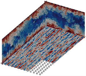
We begin by inspecting the instantaneous flow fields of representative flow cases S4_1000 and R4_1000 in figure 2, where the wall-parallel planes show contours of the streamwise velocity, and the wall-normal planes display the temperature field. The near-wall flow is populated by streaks both for the smooth and rough cases, but the roughness substantially changes the flow organization. The spacing between the roughness elements is large enough ( $2k\approx 160\delta _v$) to interfere with the canonical streaks spacing ( ${\approx }100\delta _v$), and high-speed streaks are predominantly locked between two spanwise-adjacent roughness rows, whereas low-speed streaks tend to be located on top of the roughness crests. The wall-normal planes highlight large bulges of hot fluid raising from the channel walls and protruding almost to the channel centre which are particularly evident in the cross-stream plane, whereas they get skewed in the streamwise plane under the effect of the mean shear. We note that the space between the roughness elements is primarily filled by hot fluid, whereas close to the smooth wall we can identify cold fluid patches down to the wall. Hence the roughness reduces the temperature fluctuations close to the wall. The rough wall case shows much larger temperature excursions, both at the wall and at the channel centre, which is a hint of possible effects of the roughness on the outer layer.

Figure 2. Instantaneous flow field for cases S4_1000 and R4_1000. The longitudinal and cross-stream planes show the temperature field, whereas streamwise velocity fluctuations are reported in the wall-parallel planes at  $10$ wall units from the wall (S4_1000) and from the roughness crest (R4_1000).
Another view of the instantaneous flow field is presented in figure 3, where we show the instantaneous streamwise Mach number  $u/c$ in the wall-normal planes for the smooth and rough flow cases S4_1000 and R4_1000. The smooth flow field shows a canonical organization where high-speed structures protrude down to the wall and low-speed eruptions extend towards the channel core, which is particularly evident in the cross-stream plane, figure 3(b). Over the smooth wall the flow is supersonic down to the viscous sublayer, as clear from the orange line indicating sonic conditions.

Figure 3. Instantaneous Mach number  $u/c$ for smooth flow case S4_1000 and rough wall case R4_1000 in a streamwise wall-normal plane (a,c) and a cross-stream plane (b,d). The orange isoline indicates sonic conditions $u/c=1$.
The flow organization of the rough wall case R4_1000 is substantially different from the smooth wall. The channel is essentially divided into two regions, where the high-speed core is encased by low-speed fluid close to the wall. The high-speed bundle at the channel centre appears less penetrated by the low-speed ejections from the wall as compared with the smooth wall, and the maximum Mach number is considerably higher, with localized maxima up to  $u/c\approx 8$. The sonic isoline (orange) in figure 3(c,d) shows that the roughness crests are most frequently subsonic but inrushes of high-speed fluid can penetrate down to the roughness troughs and the local Mach number is supersonic.
As common for turbulent flows the instantaneous field can be very different from the mean, and in figure 4 we show the average Mach numbers associated with the streamwise and wall-normal velocities, and the mean temperature close to the roughness element. The mean flow is effectively three-dimensional close to the roughness, especially below the crest, where we note a non-uniform spatial distribution both for the Mach number and the temperature fields, whereas the mean flow becomes homogeneous in the wall-parallel directions for  $y \gtrsim 3k$.

Figure 4. Mean flow statistics close to the roughness element: streamwise Mach number (a–e), wall-normal Mach number ( f –j) and temperature (k–o) for flow cases R2_500 (a, f ,k), R2_1000 (b,g,l), R4_500 (c,h,m), R4_1000 (d,i,n) and R03_500 (e,j,o).
The streamwise Mach number (figure 4a–e) is affected by both  $\textit {Re}_b$ and $M_b$. Increasing the Reynolds number leads to two competing effects, namely a fuller velocity profile, but also a larger $k^{+}$ and therefore a larger upward shift of the near wall cycle. In this case the latter effect is dominating. Increasing the bulk Mach number brings high speed fluid closer to the roughness, but for the cases under scrutiny the mean flow at the crest is never supersonic, although it reaches $\tilde {u}/\bar {c}\approx 0.8$ for flow cases at $M_b=4$ (figure 4c,d).
The Mach number associated with the wall-normal velocity is largely subsonic and it does not exceed  $\tilde {v}/\bar {c}\approx 0.2$, featuring extended separated flow regions both upstream and downstream of the cube because elements are in each other wakes.
The maximum mean temperature occurs at the crest height, but it is highly localized at the upstream corner of the roughness element, in correspondence of the stagnation point where the kinetic energy of the flow is converted into internal energy.
3.2. Compressibility effects on added drag
A crucial aspect of supersonic flows over roughness is whether the flow experiences the same added drag with the respect to the smooth wall across Mach numbers. The drag variation with respect to the smooth wall can be expressed as
 \begin{equation} \mathcal{DV} = 1-\frac{c_f}{c_{fs}} = 1-\frac{1}{\displaystyle\frac{R_c}{R_{cs}}\left(1-\displaystyle\frac{\Delta U^{+}}{U_{cs}^{+}}\right)^{2}} , \end{equation}
where  $c_f=2\tau _w/(\langle \bar {\rho }_c\rangle U_c^{2})$, $U_c=\langle \tilde {u}\rangle (h)$ is the mean velocity at the channel centreline, $R_c=\langle \bar {\rho }_c\rangle /\langle \bar {\rho }_w\rangle$, and the subscript $s$ denotes the smooth wall. Equation (3.1) shows that the drag variation can be related to the velocity deficit at the channel centre and in the logarithmic region,
 \begin{equation} \Delta U^{+} = U_{cs}^{+} - U_c^{+} \approx \langle \tilde{u}_s \rangle(y^{+}) - \langle\tilde{u}\rangle(y^{+}), \quad 100< y^{+}<0.3\textit{Re}_\tau \end{equation}
where the second identity is valid if outer layer similarity holds. Hence, understanding compressibility effects on  $\mathcal {DV}$ is intrinsically related to finding a compressibility transformation for the mean velocity. Moreover, a notable difference with respect to the incompressible case is the presence of the density ratio $R_c/R_{cs}$ in (3.1), which requires knowledge of the density profile.
After the celebrated velocity transformation proposed by van Driest (Reference van Driest1951), several other compressibility transformations have been developed (Trettel & Larsson Reference Trettel and Larsson2016; Volpiani et al. Reference Volpiani, Iyer, Pirozzoli and Larsson2020) aiming at improving the accuracy with reference incompressible flow data, especially for isothermal walls.
A generic compressibility transformation for the mean velocity can be expressed using stretching functions for the velocity and wall-normal coordinate,
 \begin{equation} y_I (y) = \int_0^{y} f_I(\eta)\,\mathrm{d}\eta, \quad u_I(y) = \int_0^{y} g_I(\eta)\frac{\mathrm{d} \langle\tilde{u}\rangle}{\mathrm{d}\eta}, \end{equation}
where  $f_I$ and $g_I$ for different transformations are reported in table 2. The transformed wall coordinate also allows us to define the equivalent incompressible Reynolds number,
 \begin{equation} \textit{Re}_{\tau I} = \frac{y_I(h)}{\delta_v}. \end{equation}
Table 2. Stretching functions for the generic compressibility transformation (3.3a,b) with  $R=\langle \bar {\rho }\rangle /\langle \bar {\rho }_w\rangle$ and $M=\langle \bar {\mu }\rangle /\langle \bar {\mu }_w\rangle$.

Recent compressibility transformations (Trettel & Larsson Reference Trettel and Larsson2016; Volpiani et al. Reference Volpiani, Iyer, Pirozzoli and Larsson2020) have proved their ability to account for compressibility effects and the transformed mean velocity profile over smooth walls exhibits the canonical logarithmic region,
 \begin{equation} u_{Is}^{+} = \frac{1}{\kappa}\log(y_I^{+}) + B,\quad 100< y_I^{+}<0.3Re_\tau, \end{equation}
where  $\kappa \approx 0.39$ is the von Kármán constant and $B\approx 5.1$. In the presence of wall roughness the mean velocity profile is characterized by a downward shift,
 \begin{equation} u_{I}^{+} = \frac{1}{\kappa}\log(y_I^{+}) + B - \Delta U_I^{+},\quad 100< y_I^{+}<0.3Re_\tau. \end{equation}
To verify the accuracy of compressibility transformations, figure 5 shows the mean velocity profile, untransformed (figure 5a), transformed according to van Driest (Reference van Driest1951, VD)(figure 5b), Trettel & Larsson (Reference Trettel and Larsson2016, TL)(figure 5c) and Volpiani et al. (Reference Volpiani, Iyer, Pirozzoli and Larsson2020, V)(figure 5d) for smooth (dashed) and rough wall cases (solid).

Figure 5. Mean streamwise velocity profiles for smooth (dashed) and rough (solid) wall cases. Untransformed velocity (a), van Driest-transformed velocity (van Driest Reference van Driest1951) (b), Trettel–Larsson-transformed velocity (Trettel & Larsson Reference Trettel and Larsson2016) (c) and Volpiani-transformed velocity (Volpiani et al. Reference Volpiani, Iyer, Pirozzoli and Larsson2020) (d). Rough wall cases have been shifted by  $d=0.9k$ and profiles are shown from the roughness crest upwards.
The smooth wall profiles transformed according to V show a very good agreement with the nearly incompressible flow case (dashed line with plus sign). On the contrary VD and especially TL transformations are less accurate. Rough wall cases are all characterized by the typical downward shift of the mean velocity, but we find visible compressibility effects. For instance, the supersonic cases R2_500 (red long-dashed line with solid circle) and R4_500 (red long-dashed line with solid box) show a different downward velocity shift with respect to the nearly incompressible case R03_500 (solid line with plus sign), although they share the same  $k^{+}$. We note that none of the compressibility transformations is able to account for this discrepancy. Hence, the canonical definition of roughness Reynolds number does not fully characterize the flow regime in the case of compressible flows.
As commonly done in the low-speed regime (Ibrahim et al. Reference Ibrahim, Gómez de Segura, Chung and García-Mayoral2021), rough-wall velocity profiles have been shifted to account for the effective wall origin of the flow. Over the years, several methods have been proposed to find the virtual origin, which have been recently reviewed by Chung et al. (Reference Chung, Hutchins, Schultz and Flack2021). In this study we opt for a simple option and chose  $d = 0.9k$ for all cases, which allows us to substantially reduce the uncertainty in the measure of the velocity deficit. To justify this choice in figure 6, we also report the difference between smooth and rough wall for the transformed velocity profile $u_V$ as a function of the wall distance, after shifting (dash–dotted) and before shifting (solid). The figure shows that the velocity deficits for the shifted profiles are much flatter, thus increasing the confidence in evaluating $\Delta U_I^{+}$. Throughout this work we evaluate the velocity shifts at the nominal edge of the logarithmic region $y_I^{+}=0.3{\textit {Re}_\tau }_I$.

Figure 6. Streamwise velocity deficit for Volpiani et al. (Reference Volpiani, Iyer, Pirozzoli and Larsson2020) transformation  $\langle \tilde {u}_{Vs} \rangle ^{+}$ as a function of the transformed wall distance $y^{+}_V$, at $M_b=2$ (a) and $M_b=4$ (b). Unshifted profiles are denoted with a solid line and shifted profiles with dash–dotted lines.
To understand the role of the roughness Reynolds number we cast (3.6a,b) as
 \begin{equation} u_{I}^{+} = \frac{1}{\kappa}\log(y_I/k_I) + C(k_I), \end{equation}
where  $k_I$ is the equivalent incompressible roughness height and $C(k_I)$ is a roughness dependent function. In the incompressible regime there is no ambiguity in the definition of $k_I=k$, whereas in the compressible case multiple definitions are possible and we consider two options. The first naturally stems from the compressibility transformation for the wall-normal coordinate (3.4),
 \begin{equation} k_I = y_I(k). \end{equation}
Equation (3.8) has the advantage of being consistent with the transformed velocity shift  $\Delta U_I^{+}$, however, it might be difficult to estimate it from experimental data. For this reason we also consider the following length scale:
 \begin{equation} k_* = k\frac{\langle \bar{\nu}_w\rangle}{\langle\bar{\nu}_k\rangle}, \end{equation}
where  $\bar {\nu }_k$ is the mean kinematic viscosity evaluated at the roughness crest.
Figure 7 shows the velocity shift as a function of the equivalent sand-grain roughness Reynolds number. In figure 7(a) we report the untransformed velocity shift  $\varDelta U^{+}$ as a function of $k_s^{+}$, whereas figures 7(b–d) show the transformed shift $\Delta U_I^{+}$ as a function of the corresponding $k_{sI}^{+}$. The relationship between the physical roughness height and $k_s$ for the present database was obtained by matching the nearly incompressible case R03_500 with the fully rough asymptote, which provides $k_s/k=1.9$. We also recall that the concept of sand-grain roughness Reynolds number is only valid in the fully rough regime, whereas in the transitionally rough regime different roughness geometries exhibit a different trend with $k_s^{+}$. Thakkar, Busse & Sandham (Reference Thakkar, Busse and Sandham2018) performed DNS of incompressible channel flow over grit blasted surface which shows a $\Delta U^{+}$ very similar to the data of Nikuradse (Reference Nikuradse1933) also in the transitionally rough regime. However, this is in general not expected especially for structured roughness patterns such as bars and cubes (Chung et al. Reference Chung, Hutchins, Schultz and Flack2021). The untransformed $\Delta U^{+}$ shows visible discrepancies with respect to the incompressible sand-grain roughness data of Nikuradse (Reference Nikuradse1933, crosses), and also when compared with the more recent DNS data of Abderrahaman-Elena, Fairhall & García-Mayoral (Reference Abderrahaman-Elena, Fairhall and García-Mayoral2019) for a similar roughness geometry. This is particularly evident for the transitionally rough cases, which present substantially different values of $\Delta U^{+}$, although they share the same $k_s^{+}$, figure 7(a). As for the effect of compressibility, we observe a slightly better agreement for $\varDelta U_{VD}^{+}$ in figure 7(b), but transitionally rough data at $M_b=4$ (filled square symbol) still differ from the incompressible data of Abderrahaman-Elena et al. (Reference Abderrahaman-Elena, Fairhall and García-Mayoral2019). In figure 7(b) we also report experimental data of supersonic boundary layer over rough walls, extracted from the review of Bowersox (Reference Bowersox2007), which are in good agreement with incompressible flow data and with the fully rough asymptote. However, experiments have been carried out in nearly adiabatic wall conditions (Goddard Reference Goddard1959; Latin & Bowersox Reference Latin and Bowersox2000; Ekoto et al. Reference Ekoto, Bowersox, Beutner and Goss2008), whereas the present DNS dataset is characterized by strong cooling at the wall, thus the thermodynamics properties variation at the crest is more significant and this is not accounted for by $k_s^{+}$. Figure 7(c,d) show the transformed velocity shifts $\Delta U_{TL}^{+}$ and $\Delta U_V^{+}$ as a function of the respective roughness Reynolds numbers (3.8). These transformations show similar accuracy to van Driest, and they only partially account for compressibility effects, whereas differences are still evident for the case R4_500 (filled square).

Figure 7. Shift of the mean streamwise velocity  $\Delta U^{+}$ for different compressibility transformations: untransformed (a); VD transformation (b); TL transformation (c); and V transformation (d), as a function of the corresponding equivalent sand-grain roughness Reynolds number $k_s^{+}$ and $k_{sI}^{+}$. Open symbols indicate cases at $\textit {Re}_\tau \approx 1000$, filled symbols at $\textit {Re}_\tau \approx 500$ for $M_b=2$ (circles) and $M_b=4$ (squares). In panel (b) experimental data of supersonic boundary layer are reported: Reda, Ketter & Fan (Reference Reda, Ketter and Fan1975, upward triangle); Berg (Reference Berg1979, pentagon); Goddard (Reference Goddard1959, downward triangle); (Latin & Bowersox Reference Latin and Bowersox2000, star); (Ekoto et al. Reference Ekoto, Bowersox, Beutner and Goss2008, diamond). Incompressible data are also reported: experiments of Nikuradse (Reference Nikuradse1933, crosses) and DNS of Abderrahaman-Elena et al. (Reference Abderrahaman-Elena, Fairhall and García-Mayoral2019, right triangle).
In figure 8 we report the velocity shift as a function of  $k_{*s}^{+}$, as defined in (3.9). The figure shows that the scaling based on the viscosity at the crest substantially improves the agreement with incompressible flow data, when compared with the transformed roughness height $k_I^{+}$ in figure 7.

Figure 8. Shift of the mean streamwise velocity  $\Delta U^{+}$ for different compressibility transformations: untransformed (a); VD transformation (b); TL transformation (c); and V transformation (d), as a function of the corresponding equivalent sand-grain roughness Reynolds number $k_s^{+}=1.9k^{+}$ and $k_{s*}^{+}=1.9k_*^{+}$. Open symbols indicate cases at $\textit {Re}_\tau \approx 1000$, filled symbols at $\textit {Re}_\tau \approx 500$ for $M_b=2$ (circles) and $M_b=4$ (squares). Incompressible data are also reported: experiments of Nikuradse (Reference Nikuradse1933, crosses) and DNS of Abderrahaman-Elena et al. (Reference Abderrahaman-Elena, Fairhall and García-Mayoral2019, right triangle).
When using  $k_{s*}^{+}$, we find an excellent agreement with incompressible data for all compressibility transformations (figure 8b–d), although a slightly better result is visible for $\Delta U_V^{+}$. The idea behind the length scales $k_*$ and $k_I$ is similar, namely they attempt to account for density variations between the crest and trough of the roughness, and they both seem to help the comparison with incompressible data. The transformed roughness height $k_I$ has the advantage to be consistent with its velocity transformation $\Delta U_I^{+}$, however, $k_*$ leads to slightly more accurate results, besides being easier to compute.
We believe that the definition of a relevant roughness Reynolds number  $k_I^{+}$ is a key aspect of compressible flows over roughness, but this topic has been often glossed over by previous studies, who might have involuntarily (but erroneously) incorporated this effect into $k_s^{+}$. For instance, Hill, Voisinet & Wagner (Reference Hill, Voisinet and Wagner1980) reported differences between $k_s$ of their supersonic sand-grain roughness and Nikuradse's data, and attributed the discrepancies to uncertainty in the roughness manufacturing. Another example is the work by Berg (Reference Berg1979), who carried out experiments of bar roughness at $M_\infty =6$ and computed $k_s$ by matching his $\Delta U_D^{+}$ with Nikuradse's data. In contrast our data show that calculating $k_s/k$ by matching the transformed velocity shift $\Delta U_I^{+}$ with the fully rough asymptote is not enough, because the roughness Reynolds number is also influenced by compressibility effects.
3.3. Turbulent fluctuations
We analyse the effect of surface roughness on turbulent fluctuations by decomposing the Reynolds stress tensor into a turbulent and a dispersive component as in (2.7). Figure 9 shows the streamwise Reynolds stress component  $\tau _{11}$ as a function of the viscous-scaled distance from the wall including both rough (solid lines) and smooth wall simulations (dashed lines). To facilitate comparison across Mach numbers, profiles are reported as a function of the transformed coordinate $y_{TL}^{+}$, which is usually regarded as the correct wall distance for the Reynolds stresses (Coleman et al. Reference Coleman, Kim and Moser1995; Huang, Coleman & Bradshaw Reference Huang, Coleman and Bradshaw1995).

Figure 9. Turbulent (a) and dispersive (b) streamwise Reynolds stress component as a function of  $y_{TL}^{+}$ for all flow cases. Dashed lines denote smooth wall cases and solid lines rough wall cases. Symbols in table 1.
Smooth wall data are characterized by a lack of universality even in the near wall region where the peak of  $\tau _{11}^{t}$ increases with both the Reynolds and Mach number. The former effect, widely reported also in the low-speed regime, is a consequence of the increasing relevance of outer layer structures with the Reynolds number, which provide additional energy at the low wavenumbers due to the imprinting effect on the near wall cycle (Hutchins & Marusic Reference Hutchins and Marusic2007). Instead, the latter is typically considered a genuine compressibility effect that cannot be accounted for by the density scaling (Pirozzoli & Bernardini Reference Pirozzoli and Bernardini2011).
We note that the roughness disrupts the near wall cycle and the inner peak of  $\tau _{11}^{t}$ is replaced by a much milder growth of the velocity fluctuations. The streamwise turbulent stress component has a maximum right above the crest, whose intensity is affected by both Mach and Reynolds number. At approximately matching $\textit {Re}_{\tau TL}$, we observe that the peak of $\tau _{11}^{t}$ increases with the Mach number indicating compressibility effects in proximity of the crest. We also note that at fixed Mach number the peak of $\tau _{11}^{t}$ increases with $\textit {Re}_{\tau TL}$, consistently with the incompressible flow regime.
The dispersive and turbulent stresses have approximately the same intensity below the roughness crest, whereas  $\tau _{11}^{d}$ dominates in the region $y\approx k$.
The peak of  $\tau _{11}^{d}$ occurs right below the roughness crest, and again a clear effect of compressibility is visible, with higher values for increasing Mach number. A rapid decay of the dispersive stress is observed moving away from the wall, implying that the mean flow becomes spatially homogeneous above the roughness crest.
Additional insight on the turbulence fluctuations can be gained from figure 10, where we report the turbulent and dispersive components of the Reynolds shear stress. Differently from the streamwise component, the density scaling is able to account for compressibility effects, and the main differences between cases are associated with the Reynolds number. As in the incompressible flow regime, the main effect of the roughness is to shift upwards the near wall cycle, thus the peak of  $\tau _{12}^{t}$ occurs above the crest. As for $\tau _{11}^{t}$, we observe a good match between rough and smooth wall in the channel core, which supports the validity of outer layer similarity for the velocity fluctuations. The dispersive component presents a maximum at the roughness crest, with only minor effect of the Mach number.

Figure 10. Turbulent (a) and dispersive (b) Reynolds shear stress as a function of  $y_{TL}^{+}$ for all flow cases. Dashed lines denote smooth wall cases and solid lines rough wall cases. Symbols in table 1.
To better assess compressibility effects on turbulence in figure 11 we plot the turbulent Mach number  $(\tau _{11}^{t} + \tau _{22}^{t} + \tau _{33}^{t})/\langle \bar {c}\rangle$ as a function of the wall distance for all flow cases. For the nearly incompressible case $M_t<0.05$, indicating genuine incompressible turbulence, as expected. For supersonic smooth flow cases at $M_b=2$ (figure 11a,b) the peak of $M_t$ does not exceed $0.3$, which is often considered the upper edge above which compressibility effects become relevant. Smooth flow cases at $M_b=4$ (figure 11c,d) have a slightly higher peak $M_t\approx 0.5$, indicating the increasing role of compressibility in the buffer layer, which is also reflected by the higher peak of the streamwise velocity fluctuations previously discussed.

Figure 11. Turbulent Mach number  $M_t=(\tau _{11}^{t} + \tau _{22}^{t} + \tau _{33}^{t})/\langle \bar {c}\rangle$ for flow cases R2_500, S2_500 (a), R2_1000, S2_1000 (b), R4_500, S4_500(c), R4_1000, S4_1000 (d). Nearly incompressible flow data S03_500, R03_500 are also reported in panels (a,b). Symbols in table 1.
Rough wall cases show a substantially different trend with respect to the smooth walls at all Mach numbers. Besides the obvious shift of the near wall peak, rough wall cases present much higher values of  $M_t$ and also a different shape of the profiles in the outer region, which cannot be accounted for by a simple virtual origin shift. This observation suggests that the roughness is able to affect the thermal field in the bulk flow region, as investigated in the next section, where we focus on the thermal flow statistics.
3.4. Thermal statistics
One of the peculiar features of compressible supersonic flows is the active coupling between momentum and heat transport. The study of heat transfer over rough walls has been limited to the incompressible flow regime where temperature can be considered a passive scalar (MacDonald, Hutchins & Chung Reference MacDonald, Hutchins and Chung2019; Peeters & Sandham Reference Peeters and Sandham2019), which allows direct comparison with the velocity. In the compressible case, feedback coupling between the temperature and momentum equations leads to a substantially different effect of the roughness on the thermal field.
Figure 12 shows the mean temperature profile normalized with its value at the centreline  $T_c$, as a function of the inner scaled wall distance. As typical of supersonic boundary layers with isothermal cold walls, the smooth-wall profiles exhibit a peak of the static temperature within the wall layer, at $y^{+}\approx 5$, with a positive temperature gradient at the wall, meaning that the fluid releases heat to the wall.

Figure 12. Mean temperature profile normalized by the centreline temperature as a function of the viscous-scaled distance from the wall for flow cases R2_500, S2_500 (a), R2_1000, S2_1000 (b), R4_500, S4_500 (b), R4_1000, S4_1000 (d). Dashed lines denote smooth wall cases and solid lines rough wall cases. Symbols in table 1.
The rough wall temperature profiles retain the same qualitative trend of the smooth wall cases, but they also present relevant differences. The maximum of the temperature is now located approximately at the roughness crest, and it is higher than for the smooth wall. The rough wall profiles show higher values of  $\langle \bar {T}\rangle /T_c$ over the entire wall layer, suggesting that outer layer similarity does not hold for the temperature field.
In order to understand why outer layer similarity holds for the mean velocity but not for the mean temperature we investigate the temperature–velocity relation. The coupling between the momentum and energy equations gives rise to a well known quadratic relationship between temperature and velocity (Smits & Dussauge Reference Smits and Dussauge1996), and several analytical expressions have been proposed which accurately approximate this functional form (Walz Reference Walz1959; Modesti & Pirozzoli Reference Modesti and Pirozzoli2016). A temperature–velocity relation for isothermal walls has been proposed by Zhang et al. (Reference Zhang, Bi, Hussain and She2014),
 \begin{equation} \frac{\langle\bar{T}\rangle}{T_w} = 1 + \frac{T_{rg}-T_w}{T_w}\frac{\langle\tilde{u}\rangle}{\langle\tilde{u}_c\rangle} + \frac{\langle\overline{T_c}\rangle-T_{rg}}{T_w}\left(\frac{\langle\tilde{u} \rangle}{\langle\tilde{u}_c\rangle}\right)^{2}, \end{equation}
where  $T_{rg}=\langle \overline {T_c}\rangle + r_g \langle \tilde {u}_c\rangle ^{2}/(2C_p)$, $r_g = 2 C_p (T_w-\langle \overline {T_c}\rangle ) / \langle \tilde {u}_c\rangle ^{2} - 2 Pr q_w / (\langle \tilde {u}_c\rangle \tau _w)$, and the subscript $c$ indicates quantities at the centreline.
Figure 13 shows the mean temperature as a function of the mean velocity for all flow cases, compared with the analytical relation by Zhang et al. (Reference Zhang, Bi, Hussain and She2014). For flow cases at  $M_b=2$ (figure 13a,b) the agreement between DNS data and (3.10) is excellent, for both rough and smooth wall flow cases, whereas some discrepancies are visible at higher Mach number (figure 13c,d). Despite these differences, figure 13 shows that the quadratic relation between velocity and temperature is a robust flow feature and it is also valid for rough walls. Therefore, both for rough and smooth walls it is possible to write
 \begin{equation} T^{+} = a\langle\tilde{u}\rangle^{+} + b\langle \tilde{u}\rangle^{{+}2} + T_w^{+}, \end{equation}
where  $a, b$ are parameters which depend on Mach, Reynolds number, Prandtl number and the boundary conditions. We further assume that the compressible mean velocity profiles of smooth and rough walls exhibit a logarithmic region,
 \begin{equation} \langle\tilde{u}_s\rangle^{+} = \frac{1}{\kappa'}\log(y^{+}) + B',\quad \langle\tilde{u}\rangle^{+} = \frac{1}{\kappa'}\log(y^{+}) + B'-\Delta U^{+}, \end{equation}
where  $\kappa ', B'$ are not universal as in the incompressible case but depend on the Mach number and boundary conditions. This is essentially equivalent to assuming that outer layer similarity holds for the untransformed mean velocity profile, which is a rather accurate approximation as shown in figure 5. Substituting (3.12a,b) into the respective temperature–velocity relation (3.11), and taking the difference we obtain
 \begin{equation} \langle\tilde{T}_s\rangle^{+} -\langle \bar{T}\rangle^{+} = f(y^{+}), \end{equation}
namely, unlike for the mean velocity, the difference between the smooth wall temperature and the rough wall temperature in the logarithmic region is a function of the wall distance. This clearly breaks the outer layer similarity for the mean temperature. Hence, for compressible flows over rough walls the lack of outer layer similarity can be traced back to the nonlinear relationship between the mean temperature and the mean velocity, which is a direct consequence of the aerodynamic heating. Additionally, we report the temperature fluctuations normalized by the friction temperature  $T_\tau$,
 \begin{equation} T_\tau=\frac{q_w}{\rho_wC_pu_\tau} \quad q_w = \frac{1}{2L_xL_z}\int_V \boldsymbol{\nabla} \boldsymbol{\cdot} \left(\bar{k} \boldsymbol{\nabla} \bar{T}\right)\mathrm{d}V, \end{equation}
where  $q_w$ is the heat flux per plane area.

Figure 14 shows the temperature fluctuations in viscous units for smooth- and rough-wall cases. For the smooth wall we note small values of the temperature fluctuations up to  $y^{+}\approx 10$, indicating a thicker viscous sublayer for the temperature than for velocity, and as a result the near wall peak of the temperature is shifted to $y^{+}\approx 25$– $30$.
$30$.

Figure 14. Temperature fluctuations normalized by the friction temperature  $T_\tau$ as a function of the viscous-scaled distance from the wall for smooth wall flow cases (a) and rough wall flow cases (b). Symbols in table 1.
The temperature fluctuations of the rough wall cases show a substantially different behaviour from the smooth wall. The roughness disrupts the near wall cycle and it shifts turbulence upwards, thus temperature fluctuations start increasing above the roughness crest.
The rough wall cases show the emergence of a peak of the temperature fluctuations in the outer layer, which is particularly evident for the high Reynolds number cases, figure 14(b). This peak cannot be associated with an upward shift of the near wall cycle because it occurs well into the outer layer and it increases with the Reynolds number. Therefore, we conclude that, unlike for the velocity field, the roughness is able to modify the temperature fluctuations in the outer layer.
The analysis of the one-point statistics of the temperature field reveals that  $T$ is substantially affected by the presence of the roughness, therefore it is worth comparing the wall heat flux of smooth and rough walls.
We report the wall heat flux in terms of Stanton number,
 \begin{equation} St = \frac{q_w}{\rho_bu_bC_p(T_w-T_r)} = \frac{1}{u_b^{+} (T_w^{+}-T_{r}^{+})}, \end{equation}
where  $T_r$ is the recovery temperature based on the bulk Mach number, and we compare the relative heat transfer increase with the relative drag increase using the skin-friction coefficient $C_f=2\tau _w/(\rho _b u_b^{2})$.
In figure 15(a) we report the ratio  $St/St_s$ as a function of $C_f/C_{f_s}$ and compare the present data with the case of forced convection in incompressible flows (MacDonald et al. Reference MacDonald, Hutchins and Chung2019) and to the engineering correlation of Hill et al. (Reference Hill, Voisinet and Wagner1980), developed for hypersonic flows,
 \begin{equation} \frac{St}{St_s}= \frac{C_f}{C_{fs}}\left[1+\beta\sqrt{\frac{T_w}{T_b}\frac{C_f}{2}}{k^{+}}^{0.45}Pr^{0.8} \right]^{{-}1}, \end{equation}
where  $\beta =0.4$. Note that (3.16) requires the explicit knowledge of the skin-friction coefficient of the rough case and therefore in figure 15(a) each DNS flow case (symbols in table 1) has a corresponding point evaluated with this empirical correlation (half-filled symbols).

Figure 15. (a) Stanton number as a function of the skin-friction coefficient, relative to the corresponding smooth wall values. Triangles represent incompressible flow data of forced convection of egg-cartoon roughness (MacDonald et al. Reference MacDonald, Hutchins and Chung2019). (b) Reynolds analogy factor as a function of the roughness Reynolds number compared with the hypersonic flow data by Hill et al. (Reference Hill, Voisinet and Wagner1980, black dots) over a sharp cone with grit roughness at  $M_\infty =9.9$. Smooth-wall data are also reported in panel (b), corresponding to $k^{+}=0$. Half-filled symbols refer to the values obtained from the empirical correlation (3.16) by Hill et al. (Reference Hill, Voisinet and Wagner1980) for the corresponding DNS data. Symbols style in table 1.

Figure 16. Mesh refinement study for turbulent channel flow over cubic roughness at bulk Mach number  $M_b=0.2$ and bulk Reynolds number $\textit {Re}_b=10293$. Flow case M02A (solid line) has $N_x\times N_y\times N_z=3088\times 384\times 1536$ mesh points and case M02B (circles) $N_x\times N_y\times N_z=4096\times 384\times 2048$ mesh points, corresponding to 40 and 60 grid points per roughness element, respectively.
We observe that both  $St/St_s$ and $C_f/C_{fs}>1$, namely the rough surface experiences a higher drag and heat transfer than the baseline smooth wall. The dashed line represents the Reynolds analogy line, that is the case in which the drag increase is equal to the heat transfer increase. All data lie below the axis bisector, implying that drag increases more than heat transfer, due to the additional pressure drag induced by the roughness, which does not have an equivalent for the temperature.
Our nearly incompressible flow case follows quite closely the data of egg-carton roughness by MacDonald et al. (Reference MacDonald, Hutchins and Chung2019), although these cases refer to forced thermal convection. A very similar trend holds for supersonic flow cases at  $M_b=2$ (circles), which are very close to incompressible data because aerodynamic heating plays a minor role at this Mach number. Instead, flow cases at $M_b=4$ (squares) becomes closer to the Reynolds analogy line, especially for the lower $k^{+}$, which indicates that aerodynamic heating tends to compensate for the additional pressure drag caused by the roughness. In figure 15(a) we also plot the values obtained from Hill's correlation (3.16) (half-filled symbols), which show that the empirical formula is very accurate for cases at $M_b=4$ as symbols essentially lay on top of DNS data, whereas we observe large discrepancies at $M_b=2$, especially at higher $k^{+}$.
In figure 15(b) we report the Reynolds analogy factor ( $2 St/ C_f$) as a function of the roughness Reynolds number, both for rough and smooth wall ( $k=0$) cases, and we compare DNS data with the experiments of Hill et al. (Reference Hill, Voisinet and Wagner1980) (black circles) and to the empirical formula (3.16). Smooth wall data from DNS have a Reynolds analogy factor larger than one, whereas for experimental data are closer to unity, or lower, which can be probably associated with the much higher Reynolds number of the experiments ( $\textit {Re}_\tau \approx 5000$). Despite the very different flow conditions of the experiments (higher Reynolds, $M_\infty =9$, different roughness geometry) we note a similar trend with DNS for increasing $k^{+}$, indicating that the Reynolds analogy factor mainly depends on the roughness Reynolds number.
4. Conclusions
We have presented DNSs of supersonic flows over cubical roughness elements, which are representative of the structured patterns found on the ablative shields of high-speed vehicles. We used these data to assess basic aspects of compressible flows over rough walls, which are well established in the incompressible regime, whereas they have been less explored for supersonic flows.
First, we analysed compressibility transformations and their ability to collapse the mean velocity shift onto the incompressible rough asymptote. The DNS data show that using the transformed  $\Delta U_I^{+}$ alone does not allow us to fully account for compressibility effects because of the ambiguity in defining a relevant roughness Reynolds number for the supersonic flow cases. We find important compressibility effects on the standard roughness Reynolds number $k^{+}$, which therefore is not a good candidate for comparing flows across Mach numbers. These effects have been always ignored in previous studies of supersonic flows over rough walls or, most probably, involuntarily incorporated in the equivalent roughness Reynolds number $k_s^{+}$. We propose a transformed roughness Reynolds number $k_*^{+}$ which accounts for viscosity variations between the crest and the trough, yielding excellent agreement with incompressible data, especially when used in conjunction with the recent velocity transformations by Volpiani et al. (Reference Volpiani, Iyer, Pirozzoli and Larsson2020).
Second, velocity statistics of rough and smooth walls show a very good match away from the wall, which supports the validity of outer layer similarity also for supersonic flows over rough walls. However, this does not seem to hold for the thermodynamic variables, and the temperature of rough and smooth wall cases is substantially different in the whole wall layer. We show that this can be traced back to the quadratic temperature–velocity relation which characterizes compressible flows both on smooth and rough walls.
Finally, we assessed the accuracy of the engineering correlation developed by Hill et al. (Reference Hill, Voisinet and Wagner1980) for the relative Stanton number increase with respect to a smooth wall. The accuracy of the correlation increases with the Mach number and it yields nearly perfect results already at  $M_b=4$, even if it was developed using sand-grain roughness and much higher Mach and Reynolds numbers.
This study is a first step towards the understanding of compressibility effects in flows over rough walls but it only explored a small part of the large parameter space characterizing this problem, in particular a single roughness geometry has been investigated. Future work will be dedicated to the study of different roughness geometries, as diamonds elements and sand-grain roughness, and also different wall-thermal conditions in both channel and boundary layer configurations.
DNS data are available at http://doi.org/10.4121/19403864.
Acknowledgements
We acknowledge that part of the results reported in this paper have been achieved using the PRACE Research Infrastructure resource MARCONI100 based at CINECA, Casalecchio di Reno, Italy. We also acknowledge PRACE for awarding us access to Piz Daint, at the Swiss National Supercomputing Centre (CSCS), Switzerland. D.M. is indebted to D. Chung for bringing to his attention the topic of supersonic flows over rough walls.
Declaration of interests
The authors report no conflict of interest.
Appendix. Validation of the immersed boundary method
Immersed boundary methods are known to be sensitive to the mesh resolution and often show non-monotonic grid convergence. In this study we carried out simulations using streamwise and spanwise mesh spacings which guarantee approximately 40 points inside the roughness element (i.e.  $\Delta x \approx \Delta z\approx k/40$), and used $\Delta y^{+}\approx 0.5$ below the roughness crest. In order to prove that this mesh resolution is adequate, we carried out two simulations of turbulent channel flow at bulk Mach number $M_b=0.2$ and bulk Reynolds number $Re_b=10293$ using the same computational domain of the main dataset. The first simulation M02A has $N_x\times N_y\times N_z=3088\times 384\times 1536$ mesh points, and the second M02B $N_x\times N_y\times N_z=4096\times 384\times 2048$, corresponding to 40 and 60 mesh points per roughness element, respectively. Figure 16 shows a comparison between M02A (solid) and M02B (circles) which shows that the two solutions are in nearly perfect agreement. We observe only minor deviations for the wall-normal and spanwise Reynolds stress components, but these are limited to less than $1\,\%$, and therefore, the mesh refinement study confirms that using 40 points per roughness element allows us to achieve grid independence of the flow statistics.


 Open access