


1. Introduction
It is well-known that adding a small amount of polymer additives in turbulent flows can lead to a significant drag reduction (Toms Reference Toms1948). Extensive studies have been performed to address this phenomenon in wall-bounded flows through theoretical, experimental and numerical approaches (Procaccia, L’vov & Benzi Reference Procaccia, L’vov and Benzi2008; White & Mungal Reference White and Mungal2008). However, the effects of polymer additives on heat transport in turbulent thermal convection remain less understood despite many processes involving heat transfer in nature, e.g. in oils, melts and molten magma, as well as those prevalent in industrial processes such as polymer solutions and emulsions, concerning non-Newtonian flows (Denn Reference Denn2004). These flows exhibit distinctive rheological properties, like viscoelasticity, plasticity, shear thinning and shear thickening. Among them, the viscoelastic behaviour of non-Newtonian fluids determines surprising and complex rheological properties and flow dynamics, which can lead to different unexpected fluid-flow phenomena, such as elasto-inertial turbulence (Samanta et al. Reference Samanta, Dubief, Holzner, Schafer, Morozov, Wagner and Hof2013; Li, Sureshkumar & Khomami Reference Li, Sureshkumar and Khomami2015; Sid, Terrapon & Dubief Reference Sid, Terrapon and Dubief2018; Song et al. Reference Song, Lin, Liu, Lu and Khomami2021; Dubief, Terrapon & Hof Reference Dubief, Terrapon and Hof2023) and elastic turbulence (Groisman & Steinberg Reference Groisman and Steinberg2000; Steinberg Reference Steinberg2021; Datta et al. Reference Datta2022; Song et al. Reference Song, Liu, Lu and Khomami2022, Reference Song, Lin, Zhu, Wan, Liu, Lu and Khomami2023a ,Reference Song, Zhu, Lin, Liu and Khomami b ). Therefore, studying the thermal convection in viscoelastic fluids can deepen our understanding of the interplay between the fluid viscoelasticity and convective processes. Such insights are crucial for various applications, ranging from geophysical and astrophysical phenomena such as mantle convection, to industrial processes such as polymer processing and thermal management systems.
As a canonical system to study thermal convection, Rayleigh–Bénard (RB) convection of Newtonian fluids has been studied extensively over the past decades (Bodenschatz, Pesch & Ahlers Reference Bodenschatz, Pesch and Ahlers2000; Ahlers, Grossmann & Lohse Reference Ahlers, Grossmann and Lohse2009; Lohse & Xia Reference Lohse and Xia2010; Chillà & Schumacher Reference Chillà and Schumacher2012; Xia Reference Xia2013; Shishkina Reference Shishkina2021; Lohse & Shishkina Reference Lohse and Shishkina2024). In RB convection, the flow is driven by buoyancy forces due to the temperature difference $\varDelta$
between a hot bottom plate and a cold top plate. The main dimensionless control parameters in RB convection are the Rayleigh number
$\varDelta$
between a hot bottom plate and a cold top plate. The main dimensionless control parameters in RB convection are the Rayleigh number $Ra$
, Prandtl number
$Ra$
, Prandtl number $Pr$
, and aspect ratio of the container
$Pr$
, and aspect ratio of the container $\Gamma$
, defined as
$\Gamma$
, defined as
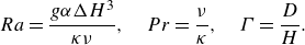 \begin{equation} Ra= \frac {g \alpha \Delta H^3}{\kappa \nu }, \quad Pr=\frac {\nu }{\kappa }, \quad \Gamma =\frac {D}{H}. \end{equation}
Here, $g$
denotes the gravitational acceleration,
$g$
denotes the gravitational acceleration, $\alpha$
the thermal expansion coefficient,
$\alpha$
the thermal expansion coefficient, $\nu$
the kinematic viscosity, and
$\nu$
the kinematic viscosity, and $\kappa$
the thermal diffusivity, and
$\kappa$
the thermal diffusivity, and $H$
and
$H$
and $D$
are the height and width of the container, respectively. Studies of this system have focused mainly on: (i) the flow structures, identifying kinetic and thermal boundary layers (BLs), and an approximately homogeneous bulk flow (Grossmann & Lohse Reference Grossmann and Lohse2000; Ahlers et al. Reference Ahlers, Grossmann and Lohse2009); and (ii) the dependence of the global heat transport, quantified by the Nusselt number
$D$
are the height and width of the container, respectively. Studies of this system have focused mainly on: (i) the flow structures, identifying kinetic and thermal boundary layers (BLs), and an approximately homogeneous bulk flow (Grossmann & Lohse Reference Grossmann and Lohse2000; Ahlers et al. Reference Ahlers, Grossmann and Lohse2009); and (ii) the dependence of the global heat transport, quantified by the Nusselt number $Nu$
, and momentum transport, characterised by the Reynolds number
$Nu$
, and momentum transport, characterised by the Reynolds number $Re$
, on the different control parameters mentioned above. The Nusselt number is defined as the ratio of the total heat flux in the flow to the molecular heat conduction, which for an incompressible flow is
$Re$
, on the different control parameters mentioned above. The Nusselt number is defined as the ratio of the total heat flux in the flow to the molecular heat conduction, which for an incompressible flow is
 \begin{equation} Nu = \frac {\left \langle u_z\theta \right \rangle _{A,t} - \kappa\, \partial _z \left \langle \theta \right \rangle _{A,t}}{\kappa \varDelta / H}. \end{equation}
Here, $u_z$
is the vertical velocity, and
$u_z$
is the vertical velocity, and $\theta$
is the temperature, while
$\theta$
is the temperature, while $\langle \cdots \rangle _{A,t}$
denotes the horizontal-plane and time average at any distance between the heated and cooled plates.
$\langle \cdots \rangle _{A,t}$
denotes the horizontal-plane and time average at any distance between the heated and cooled plates.
As regards complex fluids, some studies also considered RB convection of viscoelastic fluids, focusing on the effects of fluid elasticity on two critical Rayleigh numbers: $Ra_{c1}$
for the transition from conduction to convective flow, and
$Ra_{c1}$
for the transition from conduction to convective flow, and $Ra_{c2}$
for the onset of chaotic flows from stationary conditions. Moreover, pattern formations at small and moderate
$Ra_{c2}$
for the onset of chaotic flows from stationary conditions. Moreover, pattern formations at small and moderate $Ra$
have been studied through linear (Green Reference Green1968; Vest & Arpaci Reference Vest and Arpaci1969; Sokolov & Tanner Reference Sokolov and Tanner1972) or nonlinear stability analysis (Park & Ryu Reference Park and Ryu2001), or via numerical simulations (Wang et al. Reference Wang, Cheng, Zhang, Zheng, Cai and Siginer2023; Zheng et al. Reference Zheng, Boutaous, Xin, Siginer and Cai2023).
$Ra$
have been studied through linear (Green Reference Green1968; Vest & Arpaci Reference Vest and Arpaci1969; Sokolov & Tanner Reference Sokolov and Tanner1972) or nonlinear stability analysis (Park & Ryu Reference Park and Ryu2001), or via numerical simulations (Wang et al. Reference Wang, Cheng, Zhang, Zheng, Cai and Siginer2023; Zheng et al. Reference Zheng, Boutaous, Xin, Siginer and Cai2023).
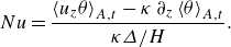
Table 1. Parameters in previous studies of turbulent RB convection with polymer additives. The fourth column gives the polymer concentration $c$
in the experiments or the viscosity ratio
$c$
in the experiments or the viscosity ratio $\beta$
in the simulations. The Weissenberg number
$\beta$
in the simulations. The Weissenberg number $Wi$
is given only for simulations (except for Benzi et al. (Reference Benzi, Ching and De Angelis2010), which defines
$Wi$
is given only for simulations (except for Benzi et al. (Reference Benzi, Ching and De Angelis2010), which defines $Wi$
using the
$Wi$
using the $\mathrm{r.m.s.}$
velocity and a large length scale of the flow in the absence of polymers, other data are adapted to the same definition using the free-fall velocity and domain height), since to measure it in experiments is challenging. In the last column, HTE means heat transfer enhancement, HTR means heat transfer reduction, and
$\mathrm{r.m.s.}$
velocity and a large length scale of the flow in the absence of polymers, other data are adapted to the same definition using the free-fall velocity and domain height), since to measure it in experiments is challenging. In the last column, HTE means heat transfer enhancement, HTR means heat transfer reduction, and $L$
is the extensibility parameter. Here, we provide only a list of literature specifically discussing the modification of the heat transfer in turbulent RB convection with polymers, while omitting numerous studies focused on pattern formation, onset of convection and other issues.
$L$
is the extensibility parameter. Here, we provide only a list of literature specifically discussing the modification of the heat transfer in turbulent RB convection with polymers, while omitting numerous studies focused on pattern formation, onset of convection and other issues.
The effect of polymer additives on turbulent RB convection has received attention only in recent years. Table 1 lists the studies of turbulent RB convection with polymer additives, and the corresponding range of parameters examined. Here, the Weissenberg number $Wi$
, which is commonly used in viscoelastic flow to quantify the elastic effects of polymer solutions, is defined as
$Wi$
, which is commonly used in viscoelastic flow to quantify the elastic effects of polymer solutions, is defined as
 \begin{equation} Wi= \frac {\lambda U}{H}, \end{equation}
where $\lambda$
is the relaxation time scale of the polymers, and
$\lambda$
is the relaxation time scale of the polymers, and $U$
is the relevant flow velocity. In terms of experimental studies, Ahlers & Nikolaenko (Reference Ahlers and Nikolaenko2010) did the first experiments at
$U$
is the relevant flow velocity. In terms of experimental studies, Ahlers & Nikolaenko (Reference Ahlers and Nikolaenko2010) did the first experiments at $Ra$
spanning from
$Ra$
spanning from $5\times 10^9$
to
$5\times 10^9$
to $10^{11}$
to investigate the turbulent heat transport modifications by polymers. They found heat transport reduction (HTR), and that HTR amount increases with polymer concentration
$10^{11}$
to investigate the turbulent heat transport modifications by polymers. They found heat transport reduction (HTR), and that HTR amount increases with polymer concentration $c$
up to
$c$
up to $10\,\%$
. Later, RB convection with polyethylene oxide (PEO) solutions was studied for
$10\,\%$
. Later, RB convection with polyethylene oxide (PEO) solutions was studied for $Ra \sim 10^9$
and
$Ra \sim 10^9$
and $Pr \approx 4.34$
for both smooth and rough plates (Wei, Ni & Xia Reference Wei, Ni and Xia2012). In the smooth cell, HTR was observed, whereas heat transport enhancement (HTE) was found in the rough cell. Moreover, a maximum HTR saturation state was observed as polymer concentration
$Pr \approx 4.34$
for both smooth and rough plates (Wei, Ni & Xia Reference Wei, Ni and Xia2012). In the smooth cell, HTR was observed, whereas heat transport enhancement (HTE) was found in the rough cell. Moreover, a maximum HTR saturation state was observed as polymer concentration $c$
increases. Based on these observations, Xie et al. (Reference Xie, Huang, Funfschilling, Li, Ni and Xia2015) further analysed the HTE mechanism within the rough cell. Their analysis revealed that the polymer additives can enhance coherent heat fluxes while suppressing incoherent heat fluxes within the bulk region, leading to the HTE. In the BL region, the plume emission rate is strongly suppressed. Thus whether HTE or HTR takes place depends on the competition between these two effects. Cai et al. (Reference Cai, Wei, Tang, Liu, Li and Li2019) found HTR in their experiments at similar
$c$
increases. Based on these observations, Xie et al. (Reference Xie, Huang, Funfschilling, Li, Ni and Xia2015) further analysed the HTE mechanism within the rough cell. Their analysis revealed that the polymer additives can enhance coherent heat fluxes while suppressing incoherent heat fluxes within the bulk region, leading to the HTE. In the BL region, the plume emission rate is strongly suppressed. Thus whether HTE or HTR takes place depends on the competition between these two effects. Cai et al. (Reference Cai, Wei, Tang, Liu, Li and Li2019) found HTR in their experiments at similar $Ra\sim 10^9$
, and concluded that the reduction is related to the smaller size of large-scale circulation (LSC) in polymer solutions. In a recent study, Xu et al. (Reference Xu, Liu, Li and Xia2025) also found an HTR in a cylindrical cell, and revealed that the addition of polymers re-establishes the cylindrical symmetry of the large-scale structures, leading to a larger flow coherence.
$Ra\sim 10^9$
, and concluded that the reduction is related to the smaller size of large-scale circulation (LSC) in polymer solutions. In a recent study, Xu et al. (Reference Xu, Liu, Li and Xia2025) also found an HTR in a cylindrical cell, and revealed that the addition of polymers re-establishes the cylindrical symmetry of the large-scale structures, leading to a larger flow coherence.
As mentioned above, the HTR saturate state was observed in high- $Ra$
experiments (Wei et al. Reference Wei, Ni and Xia2012; Cai et al. Reference Cai, Wei, Tang, Liu, Li and Li2019). This behaviour is reminiscent of the maximum drag reduction (MDR) asymptote caused by polymer additives in other wall-bounded turbulent flows, such as channel, pipe and plane Couette flows (Toms Reference Toms1948; Lumley Reference Lumley1969; Virk Reference Virk1975). The cornerstone work by Samanta et al. (Reference Samanta, Dubief, Holzner, Schafer, Morozov, Wagner and Hof2013) proposed that the dynamics of MDR is driven by an elasto-inertial instability that can even eliminate the Newtonian turbulence, and the MDR asymptote flow state can be interpreted as a self-sustained elasto-inertial turbulence, where the polymer stretching acts to suppress the small-scale vortices and turbulent fluctuations. This interpretation has gained traction, while it is not yet conclusive that the MDR asymptote is solely governed by elasto-inertial turbulence (Dubief et al. Reference Dubief, Terrapon and Hof2023). In addition, the kinetic energy spectrum in the elasto-inertial turbulence has a scaling exponent approximately
$Ra$
experiments (Wei et al. Reference Wei, Ni and Xia2012; Cai et al. Reference Cai, Wei, Tang, Liu, Li and Li2019). This behaviour is reminiscent of the maximum drag reduction (MDR) asymptote caused by polymer additives in other wall-bounded turbulent flows, such as channel, pipe and plane Couette flows (Toms Reference Toms1948; Lumley Reference Lumley1969; Virk Reference Virk1975). The cornerstone work by Samanta et al. (Reference Samanta, Dubief, Holzner, Schafer, Morozov, Wagner and Hof2013) proposed that the dynamics of MDR is driven by an elasto-inertial instability that can even eliminate the Newtonian turbulence, and the MDR asymptote flow state can be interpreted as a self-sustained elasto-inertial turbulence, where the polymer stretching acts to suppress the small-scale vortices and turbulent fluctuations. This interpretation has gained traction, while it is not yet conclusive that the MDR asymptote is solely governed by elasto-inertial turbulence (Dubief et al. Reference Dubief, Terrapon and Hof2023). In addition, the kinetic energy spectrum in the elasto-inertial turbulence has a scaling exponent approximately $-14/3$
, which is distinctly different from the Kolmogorov scaling
$-14/3$
, which is distinctly different from the Kolmogorov scaling $-5/3$
for inertial turbulence, but close to the scaling for elastic turbulence
$-5/3$
for inertial turbulence, but close to the scaling for elastic turbulence $-3.5$
; see Groisman & Steinberg (Reference Groisman and Steinberg2000), Fouxon & Lebedev (Reference Fouxon and Lebedev2003), Dubief, Terrapon & Soria (Reference Dubief, Terrapon and Soria2013) and Steinberg (Reference Steinberg2019). However, this spectral universality and associated turbulent dynamics of elasto-inertial turbulence have not been examined in natural thermal convection systems so far.
$-3.5$
; see Groisman & Steinberg (Reference Groisman and Steinberg2000), Fouxon & Lebedev (Reference Fouxon and Lebedev2003), Dubief, Terrapon & Soria (Reference Dubief, Terrapon and Soria2013) and Steinberg (Reference Steinberg2019). However, this spectral universality and associated turbulent dynamics of elasto-inertial turbulence have not been examined in natural thermal convection systems so far.
Regarding the numerical studies, polymer chains in turbulent flows are generally modelled as dumbbells composed of two beads connected by the elastic Hookean linear spring Oldrold-B model with an infinite extensibility or a nonlinear elastic entropic spring with finite extensibility, which is known as the finitely extensible nonlinear elastic-Peterlin (FENE-P) model (Bird et al. Reference Bird, Curtiss, Armstrong and Hassager1987). The FENE-P model can overcome several limitations of the Oldroyd-B model, including: (i) the possibility of singular extensional viscosity or stress in extensional flows, due to the absence of an upper bound on the polymer extensibility; (ii) the inability to reproduce the shear-thinning behaviour commonly observed in most polymer solutions (Dubief et al. Reference Dubief, Terrapon and Hof2023).
In the pioneering work of Benzi, Ching & De Angelis (Reference Benzi, Ching and De Angelis2010), homogeneous turbulent thermal convection with polymer additives was studied using direct numerical simulations (DNS) based on the FENE-P model, and then a simplified shell model was used to understand the phenomenon. The DNS were performed under periodic boundary conditions driven by a constant temperature gradient, which mimics the bulk region of RB convection, and the HTE were observed for $Wi\lt 1$
. With shell model caculations, a transition from HTE to HTR at
$Wi\lt 1$
. With shell model caculations, a transition from HTE to HTR at $Wi\gt 1$
was obtained with increasing
$Wi\gt 1$
was obtained with increasing $Wi$
. These authors speculated that the addition of polymers would increase the drag within the BL, leading to a decrease in
$Wi$
. These authors speculated that the addition of polymers would increase the drag within the BL, leading to a decrease in $Nu$
. The overall modulation of the heat transfer would then depend on the balance between the contribution from the BLs and bulk region. Moreover, they highlighted three intriguing and promising approaches to observe HTE: (i) increasing
$Nu$
. The overall modulation of the heat transfer would then depend on the balance between the contribution from the BLs and bulk region. Moreover, they highlighted three intriguing and promising approaches to observe HTE: (i) increasing $Ra$
, where heat transfer becomes dominated by the bulk region; (ii) artificially reducing the energy dissipation contribution from the BL, which is the approach explored in the experimental work of Xie et al. (Reference Xie, Huang, Funfschilling, Li, Ni and Xia2015) and already validated by their studies; and (iii) utilising a slender domain to shift the the main transport towards the bulk region.
$Ra$
, where heat transfer becomes dominated by the bulk region; (ii) artificially reducing the energy dissipation contribution from the BL, which is the approach explored in the experimental work of Xie et al. (Reference Xie, Huang, Funfschilling, Li, Ni and Xia2015) and already validated by their studies; and (iii) utilising a slender domain to shift the the main transport towards the bulk region.
Later, Benzi, Ching & De Angelis (Reference Benzi, Ching and De Angelis2016a
) performed simulations over a range of $Wi$
from
$Wi$
from $0$
to
$0$
to $50$
, at
$50$
, at $Ra=2.07\times 10^5$
,
$Ra=2.07\times 10^5$
, $Pr=7$
, by using the Oldroyd-B model. They observed HTE, and that the HTE amount first increases and then decreases with increasing
$Pr=7$
, by using the Oldroyd-B model. They observed HTE, and that the HTE amount first increases and then decreases with increasing $Wi$
, which was attributed to the combined effects of decreasing viscous energy dissipation and increasing energy dissipation due to the polymers. Cheng et al. (Reference Cheng, Zhang, Cai, Li and Li2017) explored a range of
$Wi$
, which was attributed to the combined effects of decreasing viscous energy dissipation and increasing energy dissipation due to the polymers. Cheng et al. (Reference Cheng, Zhang, Cai, Li and Li2017) explored a range of $Wi$
from
$Wi$
from $0$
to
$0$
to $10$
within a two-dimensional enclosed RB cell with Oldroyd-B polymers at
$10$
within a two-dimensional enclosed RB cell with Oldroyd-B polymers at $Ra=10^8$
and
$Ra=10^8$
and $Pr=0.7$
. These authors observed that the HTR behaves non-monotonically with
$Pr=0.7$
. These authors observed that the HTR behaves non-monotonically with $Wi$
(first increasing and then decreasing). They concluded that this non-monotonic behaviour results primarily from the contribution of elastic stresses to the turbulent kinetic energy, which absorbs energy from the turbulence for small
$Wi$
(first increasing and then decreasing). They concluded that this non-monotonic behaviour results primarily from the contribution of elastic stresses to the turbulent kinetic energy, which absorbs energy from the turbulence for small $Wi$
, while releasing stored energy to small-scale motions for relatively large
$Wi$
, while releasing stored energy to small-scale motions for relatively large $Wi$
. Dubief & Terrapon (Reference Dubief and Terrapon2020) investigated the effects of the FENE-P polymer chain extensibility parameter
$Wi$
. Dubief & Terrapon (Reference Dubief and Terrapon2020) investigated the effects of the FENE-P polymer chain extensibility parameter $L$
. In their simulations,
$L$
. In their simulations, $Wi$
ranges from 0 to 45, and
$Wi$
ranges from 0 to 45, and $L$
spans from 10 to 100 at
$L$
spans from 10 to 100 at $Ra=10^5$
,
$Ra=10^5$
, $Pr=7$
. They reported that polymers with small
$Pr=7$
. They reported that polymers with small $L$
lead to HTE, whereas polymers with larger
$L$
lead to HTE, whereas polymers with larger $L$
(
$L$
( $L\gtrsim 50$
) result in HTR. The mechanism underlying HTE involves an increase in the number of convection cells, while in the case of HTR, the LSC slows down simultaneously. Recently, Wang et al. (Reference Wang, Cheng, Zhang, Zheng, Cai and Siginer2023) found similar HTR for additional configurations at lower
$L\gtrsim 50$
) result in HTR. The mechanism underlying HTE involves an increase in the number of convection cells, while in the case of HTR, the LSC slows down simultaneously. Recently, Wang et al. (Reference Wang, Cheng, Zhang, Zheng, Cai and Siginer2023) found similar HTR for additional configurations at lower $Ra$
, except for some particular parameters where multiple pairs of LSC exist, leading to HTE.
$Ra$
, except for some particular parameters where multiple pairs of LSC exist, leading to HTE.
In all these studies, based on simulations and experiments, researchers speculated that the effects of polymers on the BL and bulk regions differ significantly. Whether the total heat transfer is enhanced or reduced depends mainly on the contributions of these two regions. To elucidate the effects of polymers on a laminar BL flow, Benzi, Ching & Chu (Reference Benzi, Ching and Chu2012) generalised the classical Prandtl–Blasius–Pohlhausen theory to Oldroyd-B viscoelatic flows at moderate $Ra$
. Their analysis demonstrated that the stretching of polymers induces a space-dependent effective viscosity, increasing near the plate, and vanishing away from it. Such an increase leads to an enhancement of friction drag, and thus results in the reduction of the heat transport in the BL region. Moreover, the effective viscosity increases with
$Ra$
. Their analysis demonstrated that the stretching of polymers induces a space-dependent effective viscosity, increasing near the plate, and vanishing away from it. Such an increase leads to an enhancement of friction drag, and thus results in the reduction of the heat transport in the BL region. Moreover, the effective viscosity increases with $Wi$
and viscosity ratio
$Wi$
and viscosity ratio $\gamma$
, therefore the amount of the HTR and drag enhancement increases as well. Here,
$\gamma$
, therefore the amount of the HTR and drag enhancement increases as well. Here, $\gamma$
is the ratio of polymer viscosity to zero-shear-rate viscosity of polymer solutions (
$\gamma$
is the ratio of polymer viscosity to zero-shear-rate viscosity of polymer solutions ( $\gamma =1-\beta$
, where
$\gamma =1-\beta$
, where $\beta$
is used in our simulation, as defined below.) Later, Benzi et al. (Reference Benzi, Ching, Yu and Wang2016b
) extended their theoretical framework to FENE-P modelled polymer solutions. They suggested that HTR occurs for polymers with large extensibility parameter
$\beta$
is used in our simulation, as defined below.) Later, Benzi et al. (Reference Benzi, Ching, Yu and Wang2016b
) extended their theoretical framework to FENE-P modelled polymer solutions. They suggested that HTR occurs for polymers with large extensibility parameter $L$
, while HTE should be observed for small
$L$
, while HTE should be observed for small $L$
. Moreover, they concluded that heat transport is enhanced when the region of substantial polymer stretching moves outside the thermal BL. These conclusions have been confirmed by Dubief & Terrapon (Reference Dubief and Terrapon2020) at low Rayleigh number
$L$
. Moreover, they concluded that heat transport is enhanced when the region of substantial polymer stretching moves outside the thermal BL. These conclusions have been confirmed by Dubief & Terrapon (Reference Dubief and Terrapon2020) at low Rayleigh number $Ra = 10^5$
, where they observed that in cases of HTE, the first normal stress difference is predominantly concentrated inside the plumes within the bulk region, while in cases of HTR, the magnitudes of the first normal stress difference inside the plumes and BL are similar. However, we have not found any evidence of this phenomenon at high
$Ra = 10^5$
, where they observed that in cases of HTE, the first normal stress difference is predominantly concentrated inside the plumes within the bulk region, while in cases of HTR, the magnitudes of the first normal stress difference inside the plumes and BL are similar. However, we have not found any evidence of this phenomenon at high $Ra$
in the literature.
$Ra$
in the literature.
As summarised in table 1, previous experimental investigations have focused primarily on high- $Ra$
(
$Ra$
( $10^9{\sim}10^{10}$
) situations, whereas simulations in the existing literature have been limited predominantly to lower
$10^9{\sim}10^{10}$
) situations, whereas simulations in the existing literature have been limited predominantly to lower $Ra$
values, typically smaller than
$Ra$
values, typically smaller than $10^6$
, due to the difficulties associated with the numerical simulations of viscoelastic flows (Alves, Oliveira & Pinho Reference Alves, Oliveira and Pinho2021). This leads to a gap in
$10^6$
, due to the difficulties associated with the numerical simulations of viscoelastic flows (Alves, Oliveira & Pinho Reference Alves, Oliveira and Pinho2021). This leads to a gap in $Ra$
values of several orders between experimental and numerical studies. Moreover, previous numerical studies on turbulent RB convection with polymer additives focused mainly on the dependence on
$Ra$
values of several orders between experimental and numerical studies. Moreover, previous numerical studies on turbulent RB convection with polymer additives focused mainly on the dependence on $Wi$
, viscosity ratio
$Wi$
, viscosity ratio $\beta$
, or extensibility parameter
$\beta$
, or extensibility parameter $L$
, while the specific effects of
$L$
, while the specific effects of $Ra$
on the heat and momentum transfer modifications, flow structures and turbulent velocity, temperature and elastic stress statistics remain unclear. To fill this gap, we have therefore performed three-dimensional DNS over a broad range of
$Ra$
on the heat and momentum transfer modifications, flow structures and turbulent velocity, temperature and elastic stress statistics remain unclear. To fill this gap, we have therefore performed three-dimensional DNS over a broad range of $Ra$
spanning from
$Ra$
spanning from $10^6$
to
$10^6$
to $10^{10}$
at
$10^{10}$
at $Pr=4.3$
while keeping moderate
$Pr=4.3$
while keeping moderate $Wi$
, namely,
$Wi$
, namely, $Wi=5$
and
$Wi=5$
and $10$
. This work seeks to provide understanding of the role played by the Rayleigh number in turbulent RB convection of viscoelastic fluids, with particular interest in the heat-transport modifications, changes of thermal plumes and BLs, and kinetic and thermal energy dissipation rates.
$10$
. This work seeks to provide understanding of the role played by the Rayleigh number in turbulent RB convection of viscoelastic fluids, with particular interest in the heat-transport modifications, changes of thermal plumes and BLs, and kinetic and thermal energy dissipation rates.
The paper is organised as follows. The physical problem, governing equations, numerical methods and computational details are described in § 2. The flow structures and statistic profiles are shown in § 3. The polymer effects on heat flux, dissipation rate and energy spectrum are discussed separately in § 4. Finally, the main conclusions are summarised in § 5.
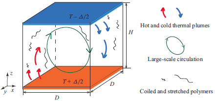
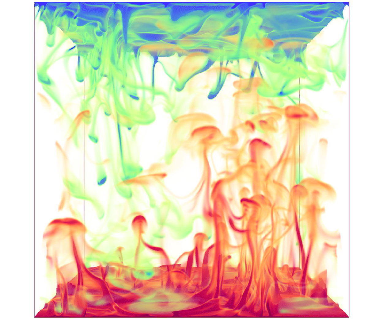
Figure 1. Sketch of viscoelastic RB convection in a parallelepiped geometry.
2. Physical problem and computational details
2.1. Governing equations
A sketch of RB convection with polymer additives in a parallelepiped geometry with $\Gamma =1$
, i.e. a cube, is shown in figure 1. The FENE-P viscoelastic constitutive model is used to model the contribution of polymer additives to the total stress. The orientation and extension of polymer molecules are described by the end-to-end vectors
$\Gamma =1$
, i.e. a cube, is shown in figure 1. The FENE-P viscoelastic constitutive model is used to model the contribution of polymer additives to the total stress. The orientation and extension of polymer molecules are described by the end-to-end vectors $q_i$
, and represented in the statistical model by the phase-averaged configuration tensor denoted by
$q_i$
, and represented in the statistical model by the phase-averaged configuration tensor denoted by $C_{ij} = \langle q_iq_j \rangle$
. The FENE-P model is frequently used in DNS of viscoelastic flows due to its physical connection with real viscoelastic liquids, specifically dilute solutions of high molecular weight, finitely extensible flexible polymers in a theta solvent. In this model, interactions between polymer chains are not considered. Although it is not easy to compare the relaxation time in the FENE-P model against real experiments, it can qualitatively capture the relevant experimental results (White & Mungal Reference White and Mungal2008; Larson & Desai Reference Larson and Desai2015; Xi Reference Xi2019; Ching Reference Ching2024; Serafini et al. Reference Serafini, Battista, Gualtieri and Casciola2024). The FENE-P model is closed by three control parameters: (i) the maximum polymer chain extensibility parameter
$C_{ij} = \langle q_iq_j \rangle$
. The FENE-P model is frequently used in DNS of viscoelastic flows due to its physical connection with real viscoelastic liquids, specifically dilute solutions of high molecular weight, finitely extensible flexible polymers in a theta solvent. In this model, interactions between polymer chains are not considered. Although it is not easy to compare the relaxation time in the FENE-P model against real experiments, it can qualitatively capture the relevant experimental results (White & Mungal Reference White and Mungal2008; Larson & Desai Reference Larson and Desai2015; Xi Reference Xi2019; Ching Reference Ching2024; Serafini et al. Reference Serafini, Battista, Gualtieri and Casciola2024). The FENE-P model is closed by three control parameters: (i) the maximum polymer chain extensibility parameter $L$
; (ii) the Weissenberg number
$L$
; (ii) the Weissenberg number $Wi$
, here defined by
$Wi$
, here defined by $Wi \equiv \lambda U_{ff} /H$
, where
$Wi \equiv \lambda U_{ff} /H$
, where $U_{ff} \equiv \sqrt {g\alpha \Delta H}$
is the characteristic free-fall velocity; and (iii) the viscosity ratio
$U_{ff} \equiv \sqrt {g\alpha \Delta H}$
is the characteristic free-fall velocity; and (iii) the viscosity ratio $\beta =\nu _s / (\nu _s+\nu _p)$
, which is the ratio of the solvent viscosity to the total zero-shear rate viscosity of the polymer solution (subscripts
$\beta =\nu _s / (\nu _s+\nu _p)$
, which is the ratio of the solvent viscosity to the total zero-shear rate viscosity of the polymer solution (subscripts $s$
and
$s$
and $p$
represent solvent and polymer, respectively). The maximum polymer chain extensibility remains constant throughout all simulations. Thus polymer chain scission is not captured in our simulations. We choose a commonly used value
$p$
represent solvent and polymer, respectively). The maximum polymer chain extensibility remains constant throughout all simulations. Thus polymer chain scission is not captured in our simulations. We choose a commonly used value $L=50$
, which implies moderate extensibility. Viscosity ratio can be regarded as a measure of polymer concentration by assuming that the viscosity depends only on the polymer concentration. In our DNS,
$L=50$
, which implies moderate extensibility. Viscosity ratio can be regarded as a measure of polymer concentration by assuming that the viscosity depends only on the polymer concentration. In our DNS, $\beta$
is fixed at
$\beta$
is fixed at $0.9$
for viscoelastic fluids (
$0.9$
for viscoelastic fluids ( $\beta =1$
for Newtonian), which denotes dilute polymer solutions.
$\beta =1$
for Newtonian), which denotes dilute polymer solutions.
The chosen reference scales for the non-dimensionalisation are the height of the domain $H$
, the temperature difference between the plates
$H$
, the temperature difference between the plates $\varDelta$
, the characteristic free-fall velocity
$\varDelta$
, the characteristic free-fall velocity $U_{ff}$
, pressure
$U_{ff}$
, pressure $\rho U_{ff}^2$
, and stress
$\rho U_{ff}^2$
, and stress $\mu _p U_{ff}/ H$
. Non-dimensional temperature
$\mu _p U_{ff}/ H$
. Non-dimensional temperature $\theta$
, velocity
$\theta$
, velocity $u_i$
(where
$u_i$
(where $i=x,y,z$
represent the three coordinate directions), pressure
$i=x,y,z$
represent the three coordinate directions), pressure $p$
, polymer stress
$p$
, polymer stress $\tau _{ij}$
and time
$\tau _{ij}$
and time $t$
are obtained by using these scales. The dimensionless governing equations for the incompressible FENE-P fluid are as follows:
$t$
are obtained by using these scales. The dimensionless governing equations for the incompressible FENE-P fluid are as follows:
 \begin{equation} \frac {\partial u_i}{\partial x_i} = 0, \end{equation}
 \begin{equation} \frac {\partial u_i}{\partial t} +u_j\frac {\partial u_i}{\partial x_j}=-\frac {\partial P}{\partial x_i}+\beta \sqrt {\frac {Pr}{Ra}} \frac {\partial ^2 u_i}{\partial x_j\,\partial x_j}+(1-\beta ) \sqrt {\frac {Pr}{Ra}}\frac {\partial \tau _{ij}}{\partial x_j}+\theta \delta _{iz}, \end{equation}
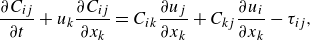 \begin{equation} \frac {\partial C_{ij}}{\partial t} + u_k\frac {\partial C_{ij}}{\partial x_k}=C_{ik}\frac {\partial u_{j}}{\partial x_k}+C_{kj}\frac {\partial u_{i}}{\partial x_k}-\tau _{ij}, \end{equation}
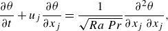 \begin{equation} \frac {\partial \theta }{\partial t} + u_j\frac {\partial \theta }{\partial x_j} = \frac {1}{\sqrt {Ra\,Pr}} \frac {\partial ^2 \theta }{\partial x_j\,\partial x_j}, \end{equation}
where the polymer stress $\tau _{ij}$
is related to the conformation tensor
$\tau _{ij}$
is related to the conformation tensor $C_{ij}$
via
$C_{ij}$
via
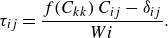 \begin{equation} \tau _{ij}=\frac {f(C_{kk})\,C_{ij}-\delta _{ij}}{Wi}. \end{equation}
The function $f(C_{kk})$
, known as the Peterlin function, is defined as
$f(C_{kk})$
, known as the Peterlin function, is defined as
 \begin{equation} f(C_{kk})=\frac {L^2-3}{L^2-C_{kk}}, \end{equation}
and $\delta _{ij}$
in (2.2) and (2.5) denotes the Kronecker symbol.
$\delta _{ij}$
in (2.2) and (2.5) denotes the Kronecker symbol.
In the above equations, the trace of the conformation tensor $C_{kk}$
represents the square of the average polymer-chain extension. It should be noted that for dilute polymer concentrations, the effect of polymer additives on the thermodynamic properties can be ignored, except for the fluid viscosity (Rubinstein & Colby Reference Rubinstein and Colby2003). No-slip boundary and constant temperature conditions are applied at the bottom and top plates, whereas periodic boundary conditions are applied in the wall-parallel horizontal directions.
$C_{kk}$
represents the square of the average polymer-chain extension. It should be noted that for dilute polymer concentrations, the effect of polymer additives on the thermodynamic properties can be ignored, except for the fluid viscosity (Rubinstein & Colby Reference Rubinstein and Colby2003). No-slip boundary and constant temperature conditions are applied at the bottom and top plates, whereas periodic boundary conditions are applied in the wall-parallel horizontal directions.
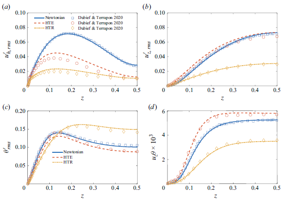
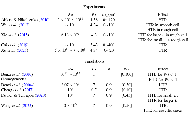
Figure 2. Comparison of statistics profiles from our simulations with the results of Dubief & Terrapon (Reference Dubief and Terrapon2020) for the Newtonian flow and non-Newtonian flows with an HTE flow state at $Wi=10$
,
$Wi=10$
, $L=25$
and an HTR flow state at
$L=25$
and an HTR flow state at $Wi=40$
,
$Wi=40$
, $L=100$
. The other control parameters are fixed at
$L=100$
. The other control parameters are fixed at $Ra=10^5$
,
$Ra=10^5$
, $Pr=7$
,
$Pr=7$
, $\beta =0.9$
and
$\beta =0.9$
and $\Gamma = 16$
. Root mean square (r.m.s.) of (a) horizontal velocity
$\Gamma = 16$
. Root mean square (r.m.s.) of (a) horizontal velocity $u^{\prime }_{h,{rms}}$
, (b) vertical velocity
$u^{\prime }_{h,{rms}}$
, (b) vertical velocity $u^{\prime }_{z,{rms}}$
, (c) temperature fluctuations
$u^{\prime }_{z,{rms}}$
, (c) temperature fluctuations $\theta _{{rms}}^{\prime }$
. (d) Mean heat flux
$\theta _{{rms}}^{\prime }$
. (d) Mean heat flux $\langle u_z\theta \rangle$
across the half-gap.
$\langle u_z\theta \rangle$
across the half-gap.
2.2. Numerical method and validations
The equations introduced above are solved via an in-house viscoelastic solver based on the open source AFiD code (Verzicco & Orlandi Reference Verzicco and Orlandi1996; van der Poel et al. Reference van der Poel, Ostilla-Mónico, Donners and Verzicco2015b
). The AFiD code is an energy-conserving second-order finite difference code that has been proven to be a versatile Navier–Stokes solver for wall-bounded turbulent flows (Verzicco & Orlandi Reference Verzicco and Orlandi1996). Moreover, the code is parallelised using a two-dimensional pencil domain decomposition strategy, allowing it to effectively handle large-scale computations (van der Poel et al. Reference van der Poel, Ostilla-Mónico, Donners and Verzicco2015b
). The code uses a staggered grid for the spatial discretization, with velocities located on the cell faces, and the other variables (pressure, conformation tensor and elastic stress) at the cell centre, except temperature, which is collocated with the vertical velocity $u_z$
. In the new version of the code, all spatial derivatives are approximated by using the second-order central finite differences except for the advection term in (2.3), where a Kurganov–Tadmor scheme (Vaithianathan et al. Reference Vaithianathan, Robert, Brasseur and Collins2006; Lin et al. Reference Lin, Wan, Zhu, Liu, Lu and Khomami2022) is used; indeed, the hyperbolic nature of this equation requires a special treatment of the convective term to ensure numerical convergence, especially at high
$u_z$
. In the new version of the code, all spatial derivatives are approximated by using the second-order central finite differences except for the advection term in (2.3), where a Kurganov–Tadmor scheme (Vaithianathan et al. Reference Vaithianathan, Robert, Brasseur and Collins2006; Lin et al. Reference Lin, Wan, Zhu, Liu, Lu and Khomami2022) is used; indeed, the hyperbolic nature of this equation requires a special treatment of the convective term to ensure numerical convergence, especially at high $Wi$
(Min, Yoo & Choi Reference Min, Yoo and Choi2001). Specifically, the Kurganov–Tadmor scheme is a modified central difference scheme that ensures the symmetric-positive-definite property of
$Wi$
(Min, Yoo & Choi Reference Min, Yoo and Choi2001). Specifically, the Kurganov–Tadmor scheme is a modified central difference scheme that ensures the symmetric-positive-definite property of $C_{ij}$
based on flux limiters. The tensor
$C_{ij}$
based on flux limiters. The tensor $C_{ij}$
at cell interfaces is constructed from the second-order, piecewise, linear approximations based on three potential candidates for approximating the gradients at cell centre: first-order forward and backward schemes, and a second-order central scheme (Vaithianathan et al. Reference Vaithianathan, Robert, Brasseur and Collins2006). In addition, a fractional-step third-order Runge–Kutta (RK3) scheme combined with a Crank–Nicolson scheme for the implicit terms is used for all the time advancements. Specifically, in (2.3), the linear stress relaxation term is treated implicitly to strictly enforce the chain finite maximum extension limit (Vaithianathan & Collins Reference Vaithianathan and Collins2003; Dubief et al. Reference Dubief, Terrapon, White, Shaqfeh, Moin and Lele2005; Song et al. Reference Song, Lin, Liu, Lu and Khomami2021). To this end, this algorithm is numerically stable and preserves the positive definiteness as well as the boundedness of the polymer conformation tensor (
$C_{ij}$
at cell interfaces is constructed from the second-order, piecewise, linear approximations based on three potential candidates for approximating the gradients at cell centre: first-order forward and backward schemes, and a second-order central scheme (Vaithianathan et al. Reference Vaithianathan, Robert, Brasseur and Collins2006). In addition, a fractional-step third-order Runge–Kutta (RK3) scheme combined with a Crank–Nicolson scheme for the implicit terms is used for all the time advancements. Specifically, in (2.3), the linear stress relaxation term is treated implicitly to strictly enforce the chain finite maximum extension limit (Vaithianathan & Collins Reference Vaithianathan and Collins2003; Dubief et al. Reference Dubief, Terrapon, White, Shaqfeh, Moin and Lele2005; Song et al. Reference Song, Lin, Liu, Lu and Khomami2021). To this end, this algorithm is numerically stable and preserves the positive definiteness as well as the boundedness of the polymer conformation tensor ( $0\lt C_{ii}\lt L^2$
).
$0\lt C_{ii}\lt L^2$
).
To validate the code, we compare our DNS results with the three-dimensional numerical simulations of Dubief & Terrapon (Reference Dubief and Terrapon2020) at $Ra=10^5$
,
$Ra=10^5$
, $Pr=7$
,
$Pr=7$
, $\beta =0.9$
and
$\beta =0.9$
and $\Gamma = 16$
using the same grid resolutions. The results of the statistical profiles for velocities, temperature and heat flux are shown in figure 2, which are in good agreement with their results. Additionally, we compared the heat transfer modification (HTM), defined as
$\Gamma = 16$
using the same grid resolutions. The results of the statistical profiles for velocities, temperature and heat flux are shown in figure 2, which are in good agreement with their results. Additionally, we compared the heat transfer modification (HTM), defined as $HTM=(Nu^V-Nu^N)/Nu^N\times 100\,\%$
. In our simulations, the HTM is
$HTM=(Nu^V-Nu^N)/Nu^N\times 100\,\%$
. In our simulations, the HTM is $14.4\,\%$
for the HTE flow state, and
$14.4\,\%$
for the HTE flow state, and $-31.4\,\%$
for the HTR flow state, closely matching their results
$-31.4\,\%$
for the HTR flow state, closely matching their results $11\,\%$
and
$11\,\%$
and $-31\,\%$
, respectively. The small quantitative differences may be attributed to the different numerical schemes, specifically the inclusion of an artificial diffusion term in their code. Moreover, the present DNS results of the heat transport modification for highly turbulent thermal convection with polymer additives agree quantitatively with previous experiments in a similar parameter range. Specifically, our DNS at
$-31\,\%$
, respectively. The small quantitative differences may be attributed to the different numerical schemes, specifically the inclusion of an artificial diffusion term in their code. Moreover, the present DNS results of the heat transport modification for highly turbulent thermal convection with polymer additives agree quantitatively with previous experiments in a similar parameter range. Specifically, our DNS at $10^{9} \leqslant Ra\leqslant 10^{10}$
,
$10^{9} \leqslant Ra\leqslant 10^{10}$
, $Pr=4.3$
give an HTR approximately
$Pr=4.3$
give an HTR approximately $9\,\%{\sim}15\,\%$
, which is quite close to the
$9\,\%{\sim}15\,\%$
, which is quite close to the $10\,\%{\sim}12\,\%$
measured in the experiments by Ahlers & Nikolaenko (Reference Ahlers and Nikolaenko2010), Wei et al. (Reference Wei, Ni and Xia2012) and Cai et al. (Reference Cai, Wei, Tang, Liu, Li and Li2019) for similar parameters
$10\,\%{\sim}12\,\%$
measured in the experiments by Ahlers & Nikolaenko (Reference Ahlers and Nikolaenko2010), Wei et al. (Reference Wei, Ni and Xia2012) and Cai et al. (Reference Cai, Wei, Tang, Liu, Li and Li2019) for similar parameters $10^{9}\leqslant Ra\leqslant 7\times 10^{10}$
,
$10^{9}\leqslant Ra\leqslant 7\times 10^{10}$
, $Pr=4.3$
. For further validation cases and details of the code, we refer to Song, Xu & Shishkina (Reference Song, Xu and Shishkina2025).
$Pr=4.3$
. For further validation cases and details of the code, we refer to Song, Xu & Shishkina (Reference Song, Xu and Shishkina2025).
2.3. Simulation parameters
In our simulations, we explore the range of $Ra$
spanning from
$Ra$
spanning from $10^6$
to
$10^6$
to $10^{10}$
at fixed
$10^{10}$
at fixed $Pr=4.3$
, corresponding to pure water at
$Pr=4.3$
, corresponding to pure water at $40\,^\circ$
C. We consider a moderate level of elasticity:
$40\,^\circ$
C. We consider a moderate level of elasticity: $Wi=5$
and
$Wi=5$
and $Wi=10$
, with
$Wi=10$
, with $Wi=0$
representing Newtonian flow.
$Wi=0$
representing Newtonian flow.
In classical Newtonian RB convection, the mesh resolution should be adequate to resolve the Kolmogorov $\eta _K^*\equiv (\nu ^3/\varepsilon _u^*)^{1/4}$
and Batchelor
$\eta _K^*\equiv (\nu ^3/\varepsilon _u^*)^{1/4}$
and Batchelor $\eta _B^*\equiv (\nu \kappa ^2/\varepsilon _u^*)^{1/4}$
length scales, where
$\eta _B^*\equiv (\nu \kappa ^2/\varepsilon _u^*)^{1/4}$
length scales, where $\varepsilon _u^*$
represents the kinetic energy dissipation rate, with
$\varepsilon _u^*$
represents the kinetic energy dissipation rate, with $^*$
indicating dimensional quantities. The dimensionless forms of these two length scales are calculated by
$^*$
indicating dimensional quantities. The dimensionless forms of these two length scales are calculated by
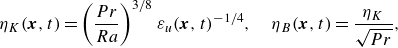 \begin{equation} {\eta _K}(\boldsymbol{x},t) = \left (\frac {Pr}{Ra}\right )^{3/8}\varepsilon _u(\boldsymbol{x},t)^{-1/4},\quad {\eta _B}(\boldsymbol{x},t) = \frac {\eta _K}{\sqrt {Pr}}, \end{equation}
where the dimensionless kinetic energy dissipation rate is given by $\varepsilon _u(\boldsymbol{x},t)=\sqrt {Pr/Ra}\,[\partial _i u_j(\boldsymbol{x},t)]^2$
(Scheel, Emran & Schumacher Reference Scheel, Emran and Schumacher2013). We ensure adequate grid resolution in all directions by requiring that the maximal value of the ratio of the mesh size to the local Kolmogorov
$\varepsilon _u(\boldsymbol{x},t)=\sqrt {Pr/Ra}\,[\partial _i u_j(\boldsymbol{x},t)]^2$
(Scheel, Emran & Schumacher Reference Scheel, Emran and Schumacher2013). We ensure adequate grid resolution in all directions by requiring that the maximal value of the ratio of the mesh size to the local Kolmogorov $h_{{max}}/{\eta _K}$
and Batchelor
$h_{{max}}/{\eta _K}$
and Batchelor $h_{{max}}/{\eta _B}$
microscales is smaller than 3, which was found empirically to be acceptable (Verzicco Reference Verzicco and Camussi2003; Shishkina et al. Reference Shishkina, Stevens, Grossmann and Lohse2010), where
$h_{{max}}/{\eta _B}$
microscales is smaller than 3, which was found empirically to be acceptable (Verzicco Reference Verzicco and Camussi2003; Shishkina et al. Reference Shishkina, Stevens, Grossmann and Lohse2010), where $h_{{max}}=\max ( \Delta x, \Delta y, \Delta z )$
. For all the cases, the mesh width fulfils these requirements (see table 2,
$h_{{max}}=\max ( \Delta x, \Delta y, \Delta z )$
. For all the cases, the mesh width fulfils these requirements (see table 2, $h_{{max}}/\eta _K$
and
$h_{{max}}/\eta _K$
and $h_{{max}}/\eta _B$
). Notably, according to Stevens, Verzicco & Lohse (Reference Stevens, Verzicco and Lohse2010), higher resolution in the horizontal direction is necessary to resolve the plume dynamics in the BL. Further, we check the number of mesh points inside the thermal and viscous BLs (see table 2,
$h_{{max}}/\eta _B$
). Notably, according to Stevens, Verzicco & Lohse (Reference Stevens, Verzicco and Lohse2010), higher resolution in the horizontal direction is necessary to resolve the plume dynamics in the BL. Further, we check the number of mesh points inside the thermal and viscous BLs (see table 2, $N_{\theta }$
and
$N_{\theta }$
and $N_v$
) to ensure adequate resolutions inside the BL. The resolutions in our DNS fully satisfy the requirements for minimal mesh points suggested by Shishkina et al. (Reference Shishkina, Stevens, Grossmann and Lohse2010).
$N_v$
) to ensure adequate resolutions inside the BL. The resolutions in our DNS fully satisfy the requirements for minimal mesh points suggested by Shishkina et al. (Reference Shishkina, Stevens, Grossmann and Lohse2010).
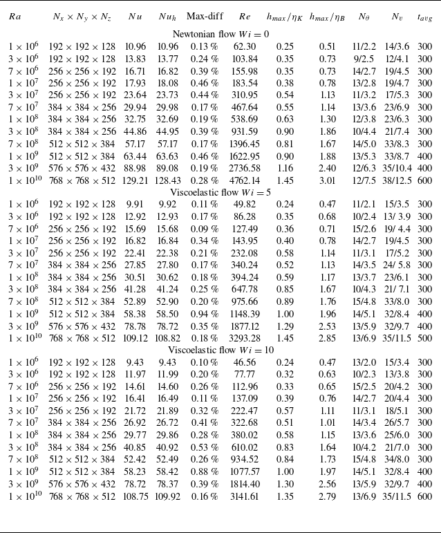
Table 2. Simulation parameters. Columns from left to right indicate $Ra$
, grid resolution, spatiotemporal averaged Nusselt number (
$Ra$
, grid resolution, spatiotemporal averaged Nusselt number ( $Nu$
) determined by averaging the results from four methods, Nusselt number
$Nu$
) determined by averaging the results from four methods, Nusselt number $Nu_h$
computed by using half of the statistical time (Stevens et al. Reference Stevens, Verzicco and Lohse2010), maximum difference between four methods (Max-diff), Reynolds number
$Nu_h$
computed by using half of the statistical time (Stevens et al. Reference Stevens, Verzicco and Lohse2010), maximum difference between four methods (Max-diff), Reynolds number $Re$
, the maximum value of the ratio of the local mesh size
$Re$
, the maximum value of the ratio of the local mesh size $h_{{max}}=\max ( \Delta x, \Delta y, \Delta z )$
to the local Kolmogorov
$h_{{max}}=\max ( \Delta x, \Delta y, \Delta z )$
to the local Kolmogorov $\eta _K$
and Batchelor
$\eta _K$
and Batchelor $ \eta _B$
length scales, the number of grid points inside the thermal BL,
$ \eta _B$
length scales, the number of grid points inside the thermal BL, $N_{\theta }$
, and viscous BL,
$N_{\theta }$
, and viscous BL, $N_{v}$
(actual resolution/requirement; Shishkina et al. Reference Shishkina, Stevens, Grossmann and Lohse2010), and the statistical averaging time
$N_{v}$
(actual resolution/requirement; Shishkina et al. Reference Shishkina, Stevens, Grossmann and Lohse2010), and the statistical averaging time $t_{{avg}}$
in the free-fall time units.
$t_{{avg}}$
in the free-fall time units.
In a viscoelastic flow, the typical length is similar or even larger than those in a Newtonian fluid (Benzi et al. Reference Benzi, Ching and De Angelis2010; Wei et al. Reference Wei, Ni and Xia2012; Cheng et al. Reference Cheng, Zhang, Cai, Li and Li2017), therefore, for viscoelastic flows we use the same mesh resolutions as in the corresponding Newtonian flows. In table 2, we similarly provide $h_{{max}}/\eta _K$
,
$h_{{max}}/\eta _K$
, $h_{{max}}/ \eta _B$
and the mesh points inside the BL with the minimal mesh points according to Shishkina et al. (Reference Shishkina, Stevens, Grossmann and Lohse2010). The Kolmogorov and Batchelor length scales are defined using the Newtonian solvent dissipation rate
$h_{{max}}/ \eta _B$
and the mesh points inside the BL with the minimal mesh points according to Shishkina et al. (Reference Shishkina, Stevens, Grossmann and Lohse2010). The Kolmogorov and Batchelor length scales are defined using the Newtonian solvent dissipation rate $\varepsilon _u^{[s]}$
, excluding polymer dissipation
$\varepsilon _u^{[s]}$
, excluding polymer dissipation $\varepsilon _u^{[p]}$
, as
$\varepsilon _u^{[p]}$
, as $\eta _K^*=(\nu _s^3/\varepsilon _u^{[s]^*})^{1/4}$
and
$\eta _K^*=(\nu _s^3/\varepsilon _u^{[s]^*})^{1/4}$
and $\eta _B^*= (\nu _s \kappa ^2/\varepsilon _u^{[s]^*})^{1/4}$
. Their dimensionless forms are
$\eta _B^*= (\nu _s \kappa ^2/\varepsilon _u^{[s]^*})^{1/4}$
. Their dimensionless forms are
 \begin{equation} {\eta _K}(\boldsymbol{x},t) = \left (\frac {Pr}{Ra}\right )^{3/8}\beta ^{3/4}\,\varepsilon _u^{[s]}(\boldsymbol{x},t)^{-1/4},\quad {\eta _B}(\boldsymbol{x},t) = \frac {\eta _K(\boldsymbol{x},t)}{\sqrt {\beta\, Pr}}, \end{equation}
where
 \begin{equation} \varepsilon _u^{[s]}=\beta \sqrt {\frac {Pr}{Ra}}\,[ \partial _i u_j(\boldsymbol{x},t) ]^2,\quad \varepsilon _u^{[p]}=-(1-\beta )\sqrt {\frac {Pr}{Ra}}\, u_i\,\partial _j \tau _{ij}. \end{equation}
To start the simulation of a Newtonian flow, the temperature field is initialised by a linear profile, and the velocity field is initialised with random fluctuation of maximum amplitude 0.001 to trigger the transition to the chaotic turbulent motion. In the viscoelastic cases, the temperature and velocity flow fields are initialised with those of the corresponding Newtonian flows in the statistically stationary state, while the initial conformation tensor is set to the unit tensor, corresponding to the equilibrium state. Statistical data are collected after the flow reaches a statistically stationary state, determined by the convergence of $Nu$
and volume-averaged turbulent kinetic energy, which typically happens after at least 500 dimensionless time units for all cases. Table 2 provides the time span
$Nu$
and volume-averaged turbulent kinetic energy, which typically happens after at least 500 dimensionless time units for all cases. Table 2 provides the time span $t_{{avg}}$
for the statistical data sampling in free-fall time units. In this paper, the statistic profiles presented in § 3.3 are further averaged over horizontal planes (
$t_{{avg}}$
for the statistical data sampling in free-fall time units. In this paper, the statistic profiles presented in § 3.3 are further averaged over horizontal planes ( $xy$
-plane), with a prime indicating fluctuations around this average.
$xy$
-plane), with a prime indicating fluctuations around this average.
We use four different methods to calculate the Nusselt number $Nu$
. One is the time and volume averaged
$Nu$
. One is the time and volume averaged $Nu$
:
$Nu$
: $Nu=1+\sqrt {Ra\, Pr} \langle u_z\theta \rangle$
. The second is derived from the exact relation for the thermal dissipation rate:
$Nu=1+\sqrt {Ra\, Pr} \langle u_z\theta \rangle$
. The second is derived from the exact relation for the thermal dissipation rate: $Nu=\sqrt {Ra\, Pr} \langle \varepsilon _\theta \rangle$
(Shraiman & Siggia Reference Shraiman and Siggia1990; Grossmann & Lohse Reference Grossmann and Lohse2000). The third and fourth values are obtained from the averages of the temperature gradients at the bottom and top plates, respectively. In table 2, the column
$Nu=\sqrt {Ra\, Pr} \langle \varepsilon _\theta \rangle$
(Shraiman & Siggia Reference Shraiman and Siggia1990; Grossmann & Lohse Reference Grossmann and Lohse2000). The third and fourth values are obtained from the averages of the temperature gradients at the bottom and top plates, respectively. In table 2, the column $Nu$
shows the average value obtained from these four methods, and the column headed ‘Max-diff’ shows the maximum difference between the results from these four methods. Notably, all differences are within 1
$Nu$
shows the average value obtained from these four methods, and the column headed ‘Max-diff’ shows the maximum difference between the results from these four methods. Notably, all differences are within 1 $\,\%$
, indicating the convergence of our simulations. We have also calculated the average
$\,\%$
, indicating the convergence of our simulations. We have also calculated the average $Nu_h$
using half of the statistical averaging time. We observe consistency between
$Nu_h$
using half of the statistical averaging time. We observe consistency between $Nu$
and
$Nu$
and $Nu_h$
for all cases, confirming that our simulations are indeed well converged, and the averaging times are sufficient. Finally, the Reynolds number
$Nu_h$
for all cases, confirming that our simulations are indeed well converged, and the averaging times are sufficient. Finally, the Reynolds number $Re$
is defined as
$Re$
is defined as $Re=U_{{rms}}\sqrt {Ra/Pr}$
, where
$Re=U_{{rms}}\sqrt {Ra/Pr}$
, where $U_{{rms}}=\sqrt {\langle u_x^2+u_y^2+u_z^2 \rangle }$
is the r.m.s. of the velocity averaged over time and the entire domain.
$U_{{rms}}=\sqrt {\langle u_x^2+u_y^2+u_z^2 \rangle }$
is the r.m.s. of the velocity averaged over time and the entire domain.
3. Results
3.1. Nusselt number and Reynolds number
We start by examining the polymer effects on the macroscopic heat and momentum transfer. Figure 3(a) presents the $Ra$
dependence of the Nusselt number
$Ra$
dependence of the Nusselt number $Nu$
compensated with
$Nu$
compensated with $Ra^{1/3}$
, and figure 3(b) presents the Reynolds number
$Ra^{1/3}$
, and figure 3(b) presents the Reynolds number $Re$
compensated with
$Re$
compensated with $Ra^{1/2}$
, where these two specific scaling exponents are suggested by Grossmann & Lohse (Reference Grossmann and Lohse2000) for the classical regime of turbulent RB convection at medium
$Ra^{1/2}$
, where these two specific scaling exponents are suggested by Grossmann & Lohse (Reference Grossmann and Lohse2000) for the classical regime of turbulent RB convection at medium $Ra$
and
$Ra$
and $Pr \gtrsim 1$
. It is evident that within our parameter ranges, both
$Pr \gtrsim 1$
. It is evident that within our parameter ranges, both $Nu$
and
$Nu$
and $Re$
are drastically reduced with the addition of polymer additives, indicating a reduction of the heat and momentum transport. Moreover, comparing to the polymer solutions with small
$Re$
are drastically reduced with the addition of polymer additives, indicating a reduction of the heat and momentum transport. Moreover, comparing to the polymer solutions with small $Wi$
(
$Wi$
( $Wi=5$
), we note that the amount of HTR and momentum transport reduction (MTR) increases at larger
$Wi=5$
), we note that the amount of HTR and momentum transport reduction (MTR) increases at larger $Wi$
(
$Wi$
( $Wi=10$
). This effect is more pronounced at the lower
$Wi=10$
). This effect is more pronounced at the lower $Ra$
under investigation, while for
$Ra$
under investigation, while for $Ra \gt 10^8$
,
$Ra \gt 10^8$
, $Nu$
is nearly the same at
$Nu$
is nearly the same at $Wi=5$
and
$Wi=5$
and $Wi=10$
, likely indicating the onset of a saturation regime. A fit to the data of Newtonian flows yields
$Wi=10$
, likely indicating the onset of a saturation regime. A fit to the data of Newtonian flows yields $Nu \sim Ra^{0.27}$
and
$Nu \sim Ra^{0.27}$
and $Re \sim Ra^{0.47}$
. In general, the data follow the theoretical scaling of the Grossmann and Lohse theory (Grossmann & Lohse Reference Grossmann and Lohse2000, Reference Grossmann and Lohse2001); see figure 3(a). With polymer additives, the scalings remain similar:
$Re \sim Ra^{0.47}$
. In general, the data follow the theoretical scaling of the Grossmann and Lohse theory (Grossmann & Lohse Reference Grossmann and Lohse2000, Reference Grossmann and Lohse2001); see figure 3(a). With polymer additives, the scalings remain similar: $Nu \sim Ra^{0.26}$
and
$Nu \sim Ra^{0.26}$
and $Re \sim Ra^{0.45}$
at
$Re \sim Ra^{0.45}$
at $Wi=5$
, and
$Wi=5$
, and $Nu \sim Ra^{0.27}$
and
$Nu \sim Ra^{0.27}$
and $Re \sim Ra^{0.46}$
at
$Re \sim Ra^{0.46}$
at $Wi=10$
, but the absolute values of
$Wi=10$
, but the absolute values of $Nu$
and
$Nu$
and $Re$
are smaller in the viscoelastic case compared to the Newtonian case. These results are consistent with previous experiments of Wei et al. (Reference Wei, Ni and Xia2012) and Cai et al. (Reference Cai, Wei, Tang, Liu, Li and Li2019); these authors found that the scalings of
$Re$
are smaller in the viscoelastic case compared to the Newtonian case. These results are consistent with previous experiments of Wei et al. (Reference Wei, Ni and Xia2012) and Cai et al. (Reference Cai, Wei, Tang, Liu, Li and Li2019); these authors found that the scalings of $Nu$
versus
$Nu$
versus $Ra$
, and
$Ra$
, and $Re$
versus
$Re$
versus $Ra$
, remain almost unchanged in their parameter ranges (
$Ra$
, remain almost unchanged in their parameter ranges ( $Ra$
span from
$Ra$
span from $10^9$
to
$10^9$
to $10^{10}$
at
$10^{10}$
at $Pr \approx 4.3$
).
$Pr \approx 4.3$
).
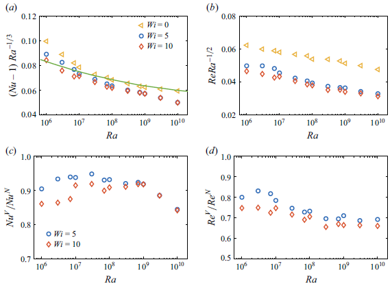
Figure 3. (a) Nusselt number $Nu-1$
compensated with
$Nu-1$
compensated with $Ra^{-1/3}$
. (b) Reynolds number
$Ra^{-1/3}$
. (b) Reynolds number $Re$
compensated with
$Re$
compensated with $Ra^{-1/2}$
. Ratios of (c)
$Ra^{-1/2}$
. Ratios of (c) $Nu$
and (d)
$Nu$
and (d) $Re$
for a viscoelastic flow to those for the corresponding Newtonian flow;
$Re$
for a viscoelastic flow to those for the corresponding Newtonian flow; $N$
and
$N$
and $V$
represent Newtonian and viscoealstic flows, respectively. The solid line in (a) is the result of the Grossmann–Lohse (Grossmann & Lohse Reference Grossmann and Lohse2000, Reference Grossmann and Lohse2001) fit for
$V$
represent Newtonian and viscoealstic flows, respectively. The solid line in (a) is the result of the Grossmann–Lohse (Grossmann & Lohse Reference Grossmann and Lohse2000, Reference Grossmann and Lohse2001) fit for $Pr=4.38$
from Ahlers et al. (Reference Ahlers2022).
$Pr=4.38$
from Ahlers et al. (Reference Ahlers2022).
Next, we directly compare $Nu$
and
$Nu$
and $Re$
of viscoelastic flows with those of Newtonian flows, as shown in figure 3(c,d). The ratio
$Re$
of viscoelastic flows with those of Newtonian flows, as shown in figure 3(c,d). The ratio $Nu^V/Nu^N$
between Newtonian and viscoelastic flows, lower than 1 for the quenching effect of polymer additives, exhibits a non-monotonic dependence on
$Nu^V/Nu^N$
between Newtonian and viscoelastic flows, lower than 1 for the quenching effect of polymer additives, exhibits a non-monotonic dependence on $Ra$
. For the Nusselt number ratio (
$Ra$
. For the Nusselt number ratio ( $Nu^V/Nu^N$
), we observe first an increase between
$Nu^V/Nu^N$
), we observe first an increase between $Ra=10^6$
and
$Ra=10^6$
and $Ra=10^7$
, followed by a slight decrease as
$Ra=10^7$
, followed by a slight decrease as $Ra$
rises further from
$Ra$
rises further from $Ra=10^7$
to
$Ra=10^7$
to $Ra=10^9$
, with a more pronounced decrease at large
$Ra=10^9$
, with a more pronounced decrease at large $Ra \geqslant 10^9$
. This non-monotonic behaviour suggests the existence of different heat transfer mechanisms in the low-
$Ra \geqslant 10^9$
. This non-monotonic behaviour suggests the existence of different heat transfer mechanisms in the low- $Ra$
and large-
$Ra$
and large- $Ra$
regions. Regarding the ratio of the Reynolds numbers (
$Ra$
regions. Regarding the ratio of the Reynolds numbers ( $Re^V/Re^N$
), a different trend is observed: a gradual decrease is noted for
$Re^V/Re^N$
), a different trend is observed: a gradual decrease is noted for $Ra\lt 10^9$
, after which it eventually reaches a plateau. It can be inferred that the polymer-induced drag enhancement becomes more pronounced with increasing
$Ra\lt 10^9$
, after which it eventually reaches a plateau. It can be inferred that the polymer-induced drag enhancement becomes more pronounced with increasing $Ra$
, and the plateau at higher
$Ra$
, and the plateau at higher $Ra$
indicates that the maximum drag enhancement due to the polymer additives has been achieved. Although there are some fluctuations in the
$Ra$
indicates that the maximum drag enhancement due to the polymer additives has been achieved. Although there are some fluctuations in the $Nu$
and
$Nu$
and $Re$
ratios at the low-
$Re$
ratios at the low- $Ra$
regime (
$Ra$
regime ( $Ra\lesssim 10^7$
), which should be attributed to the sensitivity of these quantities due to the pseudo-laminar flow state, the overall trends remain clear and consistent.
$Ra\lesssim 10^7$
), which should be attributed to the sensitivity of these quantities due to the pseudo-laminar flow state, the overall trends remain clear and consistent.
In order to compare our results with existing experiments, we note that Benzi et al. (Reference Benzi, Ching and De Angelis2016b
) provided a reference for extracting the dependence of the viscosity ratio in the FENE-P model on the polymer concentration $c$
, based on the experimental measurements of the viscosity of the PEO solution; cf. figure 7 of their paper for details. Since we have relatively large polymer extensibility, when ignoring the shear-thinning behaviour, the kinetic viscosity of the polymer solution
$c$
, based on the experimental measurements of the viscosity of the PEO solution; cf. figure 7 of their paper for details. Since we have relatively large polymer extensibility, when ignoring the shear-thinning behaviour, the kinetic viscosity of the polymer solution $\nu _{sol}(c)$
for different polymer concentrations
$\nu _{sol}(c)$
for different polymer concentrations $c$
can be simplified as the zero-shear viscosity
$c$
can be simplified as the zero-shear viscosity $\nu _s+\nu _p$
in the model. Thus we have a reasonable approximation of the relation between
$\nu _s+\nu _p$
in the model. Thus we have a reasonable approximation of the relation between $c$
and
$c$
and $\beta$
. In our DNS,
$\beta$
. In our DNS, $\beta =0.9$
would therefore correspond to the polymer concentration between 90 (ppm) and 120 (ppm). In our DNS, the ratio of
$\beta =0.9$
would therefore correspond to the polymer concentration between 90 (ppm) and 120 (ppm). In our DNS, the ratio of $Nu$
in a viscoelastic flow to that in the corresponding Newtonian flow at
$Nu$
in a viscoelastic flow to that in the corresponding Newtonian flow at $10^9 \leqslant Ra\leqslant 10^{10}$
is approximately
$10^9 \leqslant Ra\leqslant 10^{10}$
is approximately $0.85{-}0.91$
, very close to the findings of Wei et al. (Reference Wei, Ni and Xia2012), who observed ratio 0.88 for concentration
$0.85{-}0.91$
, very close to the findings of Wei et al. (Reference Wei, Ni and Xia2012), who observed ratio 0.88 for concentration $c = 120$
(ppm) at
$c = 120$
(ppm) at $Ra=8.1\times 10^9$
, to the results reported by Ahlers & Nikolaenko (Reference Ahlers and Nikolaenko2010), who found ratio 0.90 for concentration
$Ra=8.1\times 10^9$
, to the results reported by Ahlers & Nikolaenko (Reference Ahlers and Nikolaenko2010), who found ratio 0.90 for concentration $c = 120$
(ppm) at
$c = 120$
(ppm) at $Ra=6.74\times 10^{10}$
, and also to the value 0.92 for concentration
$Ra=6.74\times 10^{10}$
, and also to the value 0.92 for concentration $c = 100$
(ppm) at
$c = 100$
(ppm) at $Ra=2\times 10^{9}$
reported in Cai et al. (Reference Cai, Wei, Tang, Liu, Li and Li2019).
$Ra=2\times 10^{9}$
reported in Cai et al. (Reference Cai, Wei, Tang, Liu, Li and Li2019).
In what follows, we will focus on two key questions: first, why do the heat and momentum transport decrease, and second, why are the trends non-monotonic? Given that the results for $Wi=5$
and
$Wi=5$
and $Wi=10$
yield similar trends, our primary focus will be on the flow cases with
$Wi=10$
yield similar trends, our primary focus will be on the flow cases with $Wi=10$
.
$Wi=10$
.
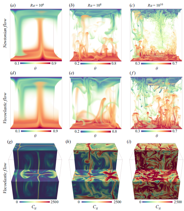
Figure 4. Instantaneous temperature fields of (a,b,c) Newtonian flows and (d,e,f) viscoelastic flows, and (g,h,i) the corresponding trace fields of viscoelastic flows. The columns from left to right represent $Ra=10^6$
,
$Ra=10^6$
, $Ra=10^8$
and
$Ra=10^8$
and $Ra=10^{10}$
, respectively. (The viewing angle of trace fields is rotated
$Ra=10^{10}$
, respectively. (The viewing angle of trace fields is rotated $30^\circ$
along the horizontal
$30^\circ$
along the horizontal $x$
-axis for a better visualisation.)
$x$
-axis for a better visualisation.)
3.2. Flow structure
The typical flow structures for both Newtonian and viscoelastic thermal convection are shown in figure 4. At low $Ra$
(
$Ra$
( $Ra=10^6$
), the Newtonian and viscoelastic flows exhibit an ascending hot plume and a descending cold plume, which generate an LSC in the bulk region (see figure 4
a,d). These plumes show quasi-periodic wave-like motions (see the supplementary movies 1 and 2) without visible horizontal sweeping. These oscillations may be attributed to plume–vortex interactions. The flow structures of the polymeric flow are similar to those of the Newtonian case, while the plumes become less wavy. With an increase of
$Ra=10^6$
), the Newtonian and viscoelastic flows exhibit an ascending hot plume and a descending cold plume, which generate an LSC in the bulk region (see figure 4
a,d). These plumes show quasi-periodic wave-like motions (see the supplementary movies 1 and 2) without visible horizontal sweeping. These oscillations may be attributed to plume–vortex interactions. The flow structures of the polymeric flow are similar to those of the Newtonian case, while the plumes become less wavy. With an increase of $Ra$
to
$Ra$
to $Ra=10^8$
(see figure 4
b), the thermal BL becomes thinner, and more plumes are ejected from the BL. The comparison between Newtonian and viscoelastic flows reveals that the polymer additives change the structure of the plumes: they become thinner, while their stems become elongated and their caps almost reach the opposite plate; see figure 4(b,e). The waviness of these plumes is substantially weakened. This is reminiscent of the flow structures characterising drag reduction in turbulent channel flows, where the near-wall streamwise streaks at the core of the turbulence self-sustaining cycle become more stable in the presence of polymer additives, a calmer phase also denoted as ’hybernation’ (Xi & Graham Reference Xi and Graham2012).
$Ra=10^8$
(see figure 4
b), the thermal BL becomes thinner, and more plumes are ejected from the BL. The comparison between Newtonian and viscoelastic flows reveals that the polymer additives change the structure of the plumes: they become thinner, while their stems become elongated and their caps almost reach the opposite plate; see figure 4(b,e). The waviness of these plumes is substantially weakened. This is reminiscent of the flow structures characterising drag reduction in turbulent channel flows, where the near-wall streamwise streaks at the core of the turbulence self-sustaining cycle become more stable in the presence of polymer additives, a calmer phase also denoted as ’hybernation’ (Xi & Graham Reference Xi and Graham2012).
At an even higher $Ra=10^{10}$
(see figure 4
c,f), the polymer additives reduce small-scale structures, making the plumes more coherent. This polymer-induced stabilisation has been reported in homogeneous turbulence (De Angelis et al. Reference De Angelis, Casciola, Benzi and Piva2005), channel and pipe flows (Dubief et al. Reference Dubief, Terrapon and Hof2023), plane Couette flow (Teng et al. Reference Teng, Liu, Lu and Khomami2018), Rayleigh–Taylor turbulence (Boffetta et al. Reference Boffetta, Mazzino, Musacchio and Vozella2010) and Taylor–Couette turbulence (Song et al. Reference Song, Lin, Zhu, Wan, Liu, Lu and Khomami2023b
).
$Ra=10^{10}$
(see figure 4
c,f), the polymer additives reduce small-scale structures, making the plumes more coherent. This polymer-induced stabilisation has been reported in homogeneous turbulence (De Angelis et al. Reference De Angelis, Casciola, Benzi and Piva2005), channel and pipe flows (Dubief et al. Reference Dubief, Terrapon and Hof2023), plane Couette flow (Teng et al. Reference Teng, Liu, Lu and Khomami2018), Rayleigh–Taylor turbulence (Boffetta et al. Reference Boffetta, Mazzino, Musacchio and Vozella2010) and Taylor–Couette turbulence (Song et al. Reference Song, Lin, Zhu, Wan, Liu, Lu and Khomami2023b
).
Finally, the bottom panels in figure 4(g,h,i) display the trace of the polymer conformation tensor, which represents the spatial distribution of the elongation of the polymer chains. We can see that at relatively low $Ra$
, most of the elongation concentrates inside the plumes, where the velocity gradient is higher, leading to maximum stretching of the polymer chains; these stretched molecules reach the opposite wall and form mushroom-like structures when interacting with the thermal BL (see the supplementary movie 3). As
$Ra$
, most of the elongation concentrates inside the plumes, where the velocity gradient is higher, leading to maximum stretching of the polymer chains; these stretched molecules reach the opposite wall and form mushroom-like structures when interacting with the thermal BL (see the supplementary movie 3). As $Ra$
increases, the magnitude of the polymer extension intensifies, and the region with highly stretched polymers becomes wider. Moreover, we also note that near the bottom/top wall, the polymers have stronger horizontal stretching at
$Ra$
increases, the magnitude of the polymer extension intensifies, and the region with highly stretched polymers becomes wider. Moreover, we also note that near the bottom/top wall, the polymers have stronger horizontal stretching at $Ra=10^8$
. For the largest
$Ra=10^8$
. For the largest $Ra=10^{10}$
case, highly stretched polymers are even more dispersed, and they can be found throughout the entire flow field.
$Ra=10^{10}$
case, highly stretched polymers are even more dispersed, and they can be found throughout the entire flow field.
To continue our analysis of the main flow features, vertical and horizontal cross-sections (mid-plane) of the temperature and trace fields are shown in figures 5 and 6, respectively. The temperature fields pertaining to the polymeric flows (second row) are directly compared with the corresponding Newtonian flow (top row), whereas the images in the bottom row depict the trace of the polymer conformation tensor. The figures clearly show that with polymer additives, the thermal BLs become thicker, and the plumes become longer, wider and less fragmented. In the core region, the polymers suppress the small-scale structures, and the temperature is less efficiently mixed, leading to more distinct plume boundaries, especially at higher $Ra$
. As concerns the polymer stretching, we note that with increasing
$Ra$
. As concerns the polymer stretching, we note that with increasing $Ra$
, the well-identified slim regions of high polymer stretching gradually become wider and more chaotic. They are seen to connect with each other and spread over the whole domain with higher intensity and finer spatial scales. The reader is also referred to the supplementary movies to better appreciate the differences in flow structures due to polymer additives.
$Ra$
, the well-identified slim regions of high polymer stretching gradually become wider and more chaotic. They are seen to connect with each other and spread over the whole domain with higher intensity and finer spatial scales. The reader is also referred to the supplementary movies to better appreciate the differences in flow structures due to polymer additives.
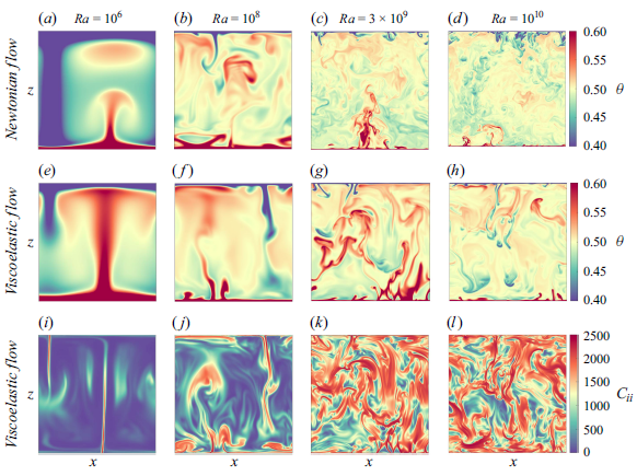
Figure 5. Instantaneous vertical cross-sections ( $xz$
-plane) of the temperature fields for (a,b,c,d) Newtonian flows, (e,f,g,h) the corresponding viscoelastic flows, and (i,j,k,l) the trace of the conformation tensor in the same cross-section. The columns from left to right represent
$xz$
-plane) of the temperature fields for (a,b,c,d) Newtonian flows, (e,f,g,h) the corresponding viscoelastic flows, and (i,j,k,l) the trace of the conformation tensor in the same cross-section. The columns from left to right represent $Ra=10^6$
,
$Ra=10^6$
, $Ra=10^8$
,
$Ra=10^8$
, $Ra=3\times 10^{9}$
and
$Ra=3\times 10^{9}$
and $Ra=10^{10}$
, respectively.
$Ra=10^{10}$
, respectively.
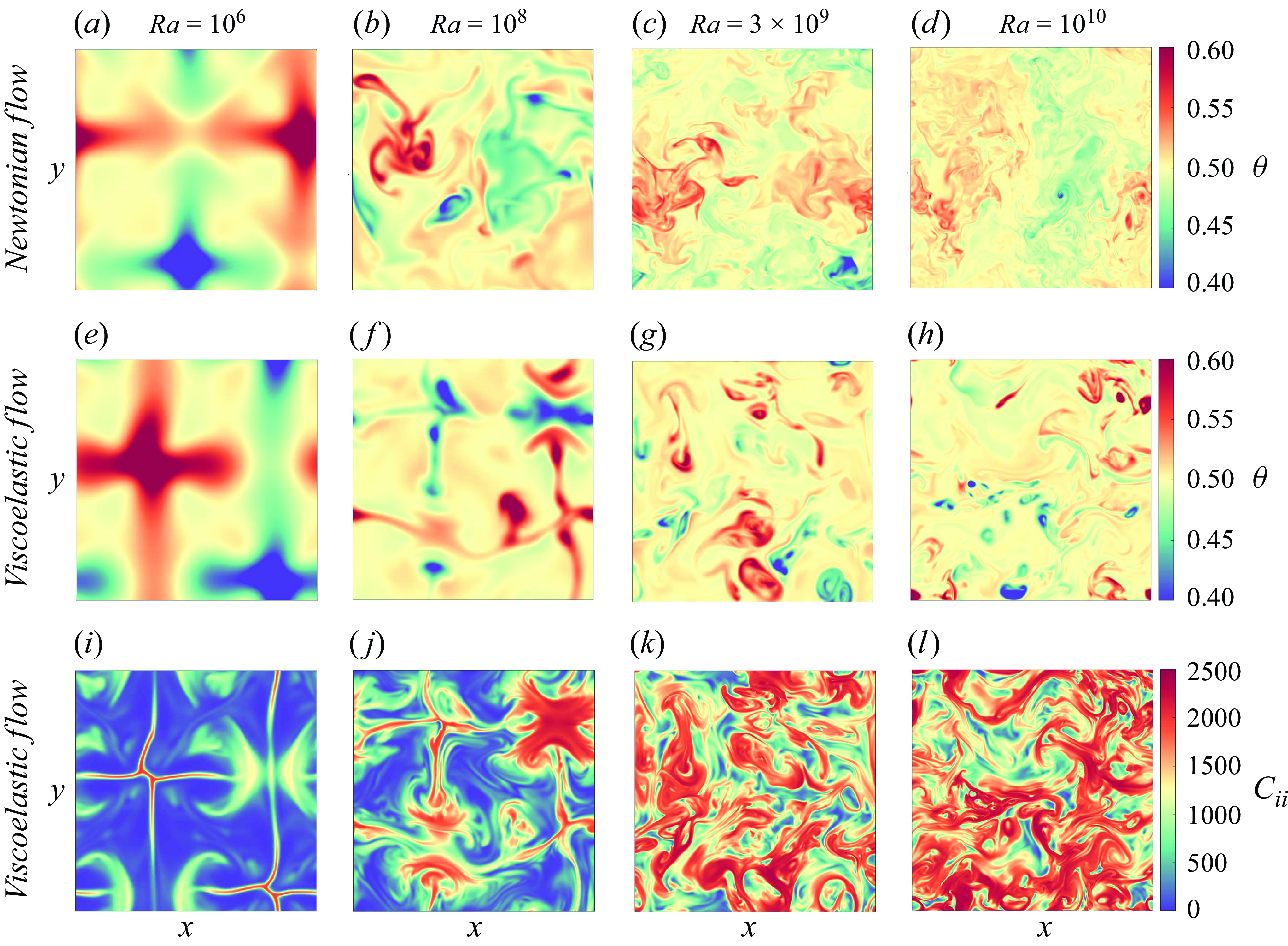
Figure 6. Instantaneous mid-height horizontal cross-sections ( $xy$
-plane) of the temperature fields for (a,b,c,d) Newtonian flows, (e,f,g,h) the corresponding viscoelastic flows, and (i,j,k,l) the trace of the conformation tensor in the same cross-section. The columns from left to right represent
$xy$
-plane) of the temperature fields for (a,b,c,d) Newtonian flows, (e,f,g,h) the corresponding viscoelastic flows, and (i,j,k,l) the trace of the conformation tensor in the same cross-section. The columns from left to right represent $Ra=10^6$
,
$Ra=10^6$
, $Ra=10^8$
,
$Ra=10^8$
, $Ra=3\times 10^{9}$
and
$Ra=3\times 10^{9}$
and $Ra=10^{10}$
, respectively.
$Ra=10^{10}$
, respectively.
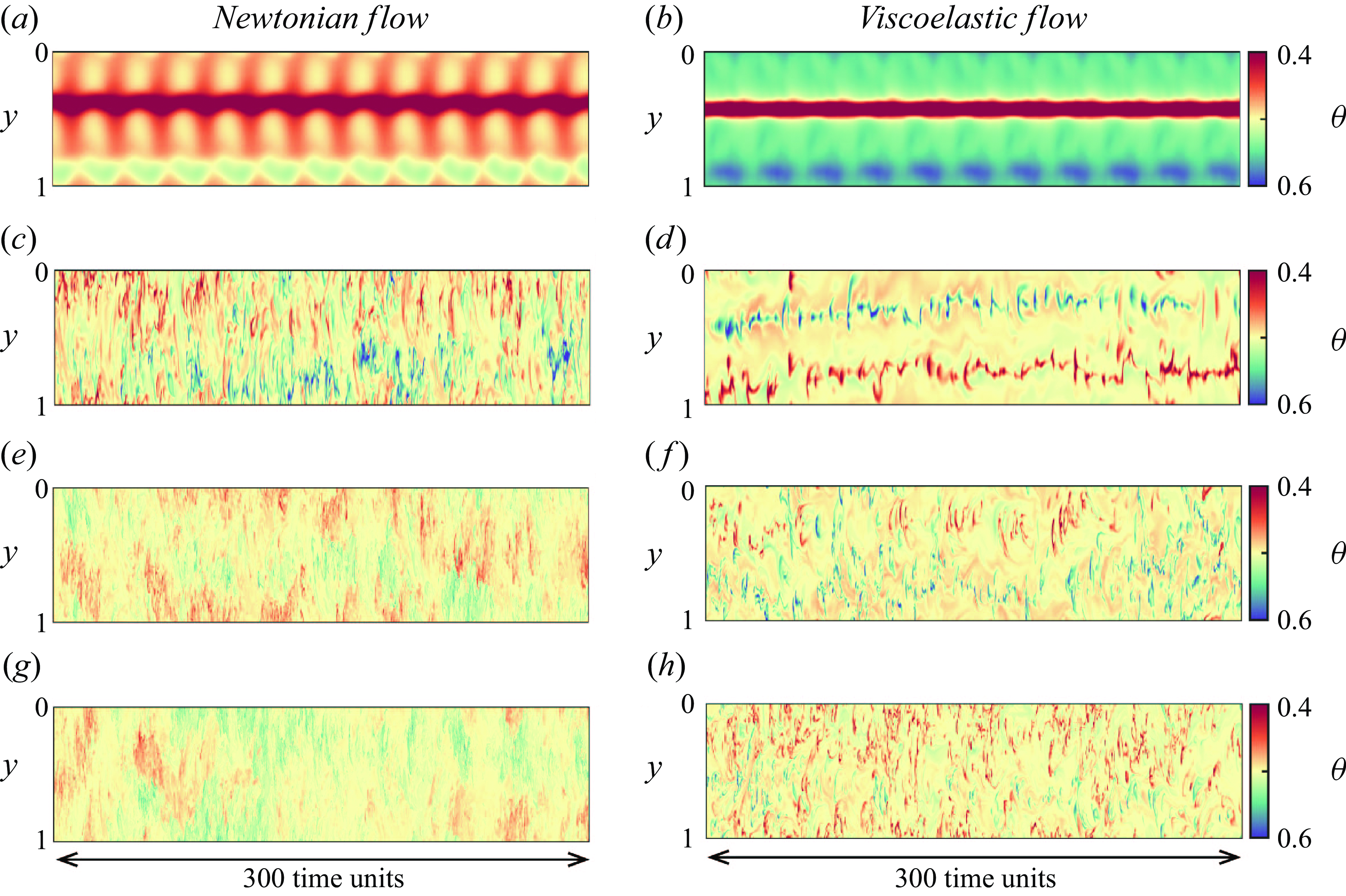
Figure 7. Temperature space–time plots for (a,c,e,g) Newtonian and (b,d,f,h) viscoelastic flows along a horizontal line $x \in [0,1]$
,
$x \in [0,1]$
, $y=0.5$
in the mid-height plane for (a,b)
$y=0.5$
in the mid-height plane for (a,b) $Ra=10^6$
, (c,d)
$Ra=10^6$
, (c,d) $Ra=10^8$
, (e,f)
$Ra=10^8$
, (e,f) $Ra=3\times 10^{9}$
, (g,h)
$Ra=3\times 10^{9}$
, (g,h) $Ra=10^{10}$
.
$Ra=10^{10}$
.
Figure 7 presents space–time plots of the temperature in Newtonian and viscoelastic flows along a horizontal line in the mid-height plane. The images are organised to show data for increasing $Ra$
in each column. In the left-hand column (figure 7
a,c,e,g), we first see that the Newtonian flow exhibits regular and periodic patterns with a stable and coherent structure. As
$Ra$
in each column. In the left-hand column (figure 7
a,c,e,g), we first see that the Newtonian flow exhibits regular and periodic patterns with a stable and coherent structure. As $Ra$
increases, the fluctuations increase, and the flow eventually exhibits a strongly chaotic behaviour. In contrast, the right-hand column (figure 7
b,d,f,h) shows that the viscoelastic flows maintain more stable and coherent structures compared to the Newtonian flows, with less variation over time. Although the turbulence intensity increases for the larger
$Ra$
increases, the fluctuations increase, and the flow eventually exhibits a strongly chaotic behaviour. In contrast, the right-hand column (figure 7
b,d,f,h) shows that the viscoelastic flows maintain more stable and coherent structures compared to the Newtonian flows, with less variation over time. Although the turbulence intensity increases for the larger $Ra\gt 10^8$
, the viscoelastic flows retain a higher coherence compared to their Newtonian counterpart. This suggests that the viscoelastic properties of the fluid help to maintain the flow stability. At an even higher
$Ra\gt 10^8$
, the viscoelastic flows retain a higher coherence compared to their Newtonian counterpart. This suggests that the viscoelastic properties of the fluid help to maintain the flow stability. At an even higher $Ra=10^{10}$
, the viscoelastic flow continues to demonstrate a stronger coherence, with reduced chaotic behaviour. Overall, the flow structures of the viscoelastic solutions exhibit a larger degree of coherence in their spatiotemporal structures compared to the corresponding Newtonian flows, as evidenced by more pronounced plume structures and less turbulent flow patterns.
$Ra=10^{10}$
, the viscoelastic flow continues to demonstrate a stronger coherence, with reduced chaotic behaviour. Overall, the flow structures of the viscoelastic solutions exhibit a larger degree of coherence in their spatiotemporal structures compared to the corresponding Newtonian flows, as evidenced by more pronounced plume structures and less turbulent flow patterns.
3.3. Turbulent and polymer statistics
In this subsection, we discuss the turbulent velocity and temperature statistics, polymeric deformation, and BL thicknesses. Figure 8 depicts the wall-normal profiles of the r.m.s. vertical $u_{z,{rms}}^{\prime }$
and horizontal
$u_{z,{rms}}^{\prime }$
and horizontal $u_{h,{rms}}^{\prime }$
velocity fluctuations for three representative cases. Both the vertical and horizontal velocity fluctuations are attenuated in the presence of polymer additives, indicating a reduction of turbulence intensity and an increase in flow drag. This observation is consistent with the HTR cases reported by Dubief & Terrapon (Reference Dubief and Terrapon2020) at
$u_{h,{rms}}^{\prime }$
velocity fluctuations for three representative cases. Both the vertical and horizontal velocity fluctuations are attenuated in the presence of polymer additives, indicating a reduction of turbulence intensity and an increase in flow drag. This observation is consistent with the HTR cases reported by Dubief & Terrapon (Reference Dubief and Terrapon2020) at $Ra=10^5$
, where the addition of polymer additives resulted in a slowdown of the LSC and thus a reduction in heat transfer.
$Ra=10^5$
, where the addition of polymer additives resulted in a slowdown of the LSC and thus a reduction in heat transfer.
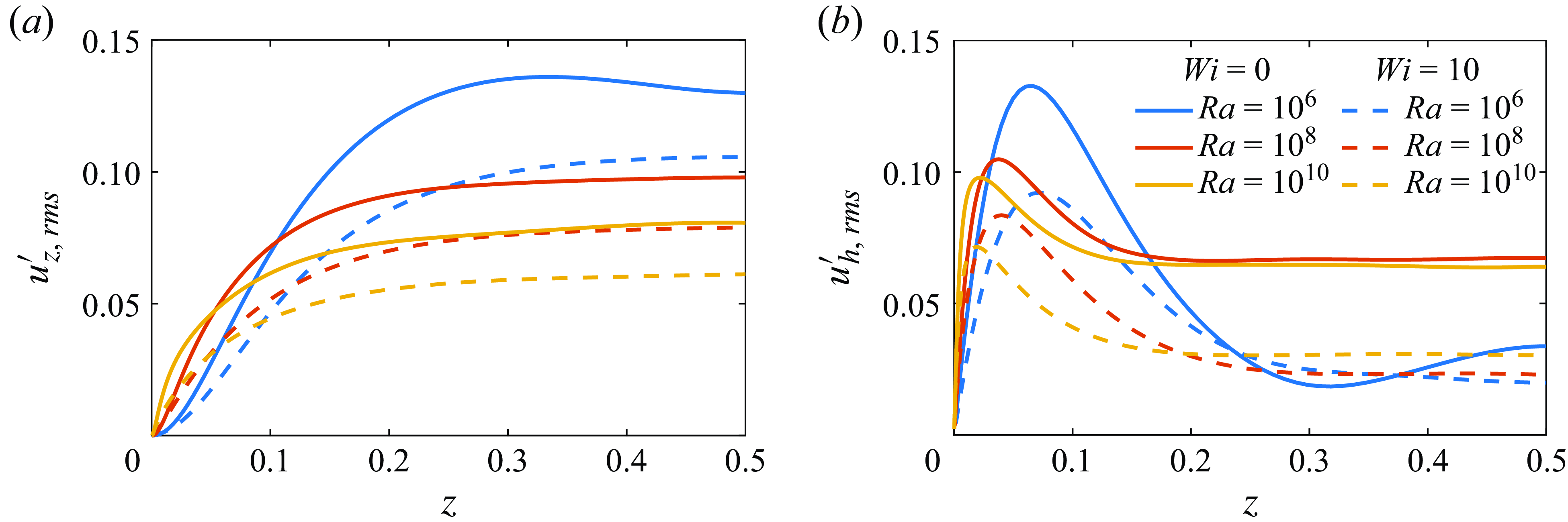
Figure 8. Intensity of the velocity fluctuations: r.m.s. profiles of (a) vertical $u_{z,{rms}}^{\prime }$
and (b) horizontal
$u_{z,{rms}}^{\prime }$
and (b) horizontal $u_{h,{rms}}^{\prime }$
velocity fluctuations for Newtonian
$u_{h,{rms}}^{\prime }$
velocity fluctuations for Newtonian $(Wi=0)$
and viscoelastic flows with
$(Wi=0)$
and viscoelastic flows with $Wi=10$
for different values of
$Wi=10$
for different values of $Ra$
.
$Ra$
.
The profiles of the mean temperature $\theta$
and r.m.s. temperature fluctuation
$\theta$
and r.m.s. temperature fluctuation $\theta ^{\prime }_{{rms}}$
for the same representative cases as in figure 8 are shown in figure 9. As
$\theta ^{\prime }_{{rms}}$
for the same representative cases as in figure 8 are shown in figure 9. As $Ra$
increases, an enhanced convection leads to the contraction of the thermal BL region, resulting in a steeper temperature gradient near the wall, and more efficient mixing within the bulk region, for both Newtonian and viscoelastic flows. From figure 9(a), we observe that the differences of mean temperature between polymeric (dashed lines) and Newtonian flows (solid lines) are small in the bulk region, where the temperature remains almost constant. Within the thermal BL, polymeric flows exhibit a slightly smoother increase of the mean temperature compared to Newtonian flows, suggesting that the addition of polymers affects the stability and structure of the thermal BL. More pronounced differences are seen in the temperature fluctuation data: in viscoelastic flows, the r.m.s. values are smaller than in Newtonian flows near the wall, and larger than those in Newtonian flows in the bulk region. The peaks of
$Ra$
increases, an enhanced convection leads to the contraction of the thermal BL region, resulting in a steeper temperature gradient near the wall, and more efficient mixing within the bulk region, for both Newtonian and viscoelastic flows. From figure 9(a), we observe that the differences of mean temperature between polymeric (dashed lines) and Newtonian flows (solid lines) are small in the bulk region, where the temperature remains almost constant. Within the thermal BL, polymeric flows exhibit a slightly smoother increase of the mean temperature compared to Newtonian flows, suggesting that the addition of polymers affects the stability and structure of the thermal BL. More pronounced differences are seen in the temperature fluctuation data: in viscoelastic flows, the r.m.s. values are smaller than in Newtonian flows near the wall, and larger than those in Newtonian flows in the bulk region. The peaks of $\theta _{{rms}}$
are lower in viscoelastic flows and located further away from the wall (which supports the idea of a thicker BL in polymer solutions). This behaviour is consistent with previous studies on polymer solutions in homogeneous turbulence (De Angelis et al. Reference De Angelis, Casciola, Benzi and Piva2005), where the polymer-induced suppression of small-scale motions is found to lead to increased fluctuations at larger scales. The reduction in temperature fluctuation near the wall implies an enhanced stability of the thermal BL, which could potentially reduce the frequency of the plume release.
$\theta _{{rms}}$
are lower in viscoelastic flows and located further away from the wall (which supports the idea of a thicker BL in polymer solutions). This behaviour is consistent with previous studies on polymer solutions in homogeneous turbulence (De Angelis et al. Reference De Angelis, Casciola, Benzi and Piva2005), where the polymer-induced suppression of small-scale motions is found to lead to increased fluctuations at larger scales. The reduction in temperature fluctuation near the wall implies an enhanced stability of the thermal BL, which could potentially reduce the frequency of the plume release.
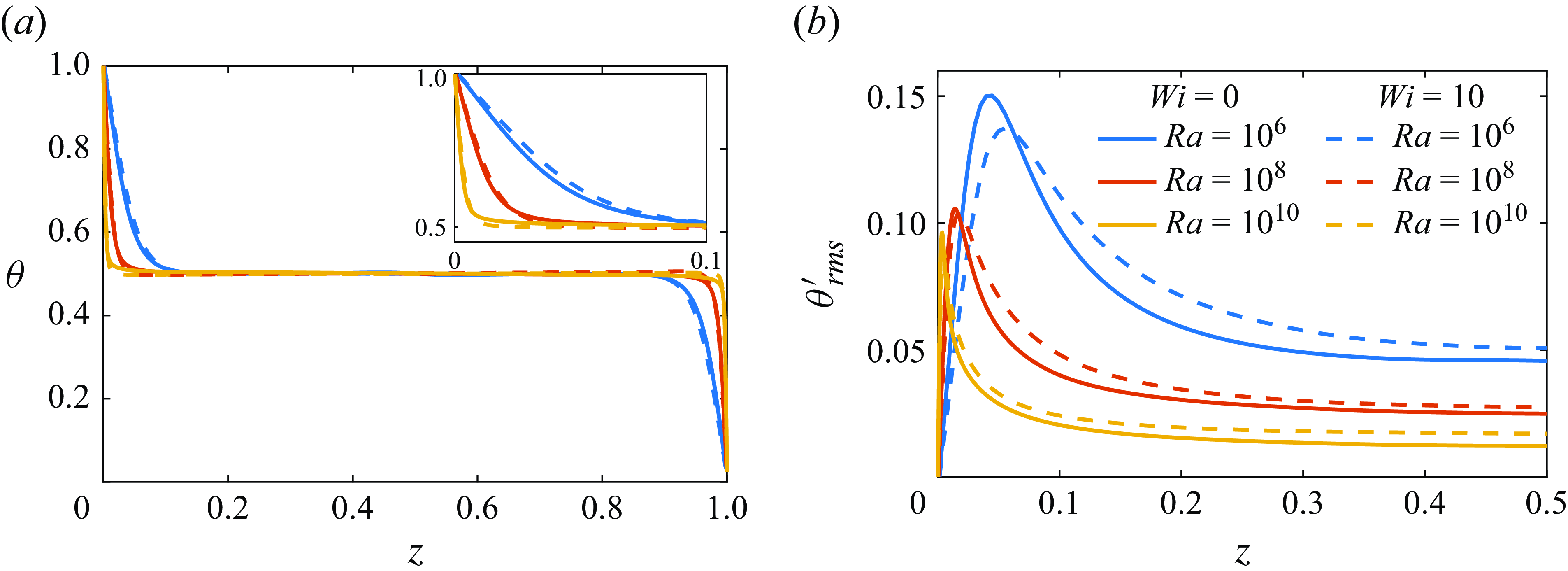
Figure 9. Profiles of (a) the average temperature $\theta$
and (b) the temperature fluctuations
$\theta$
and (b) the temperature fluctuations $\theta ^{\prime }_{{rms}}$
for different values of
$\theta ^{\prime }_{{rms}}$
for different values of $Ra$
. The inset shows the profile in the near-wall region.
$Ra$
. The inset shows the profile in the near-wall region.
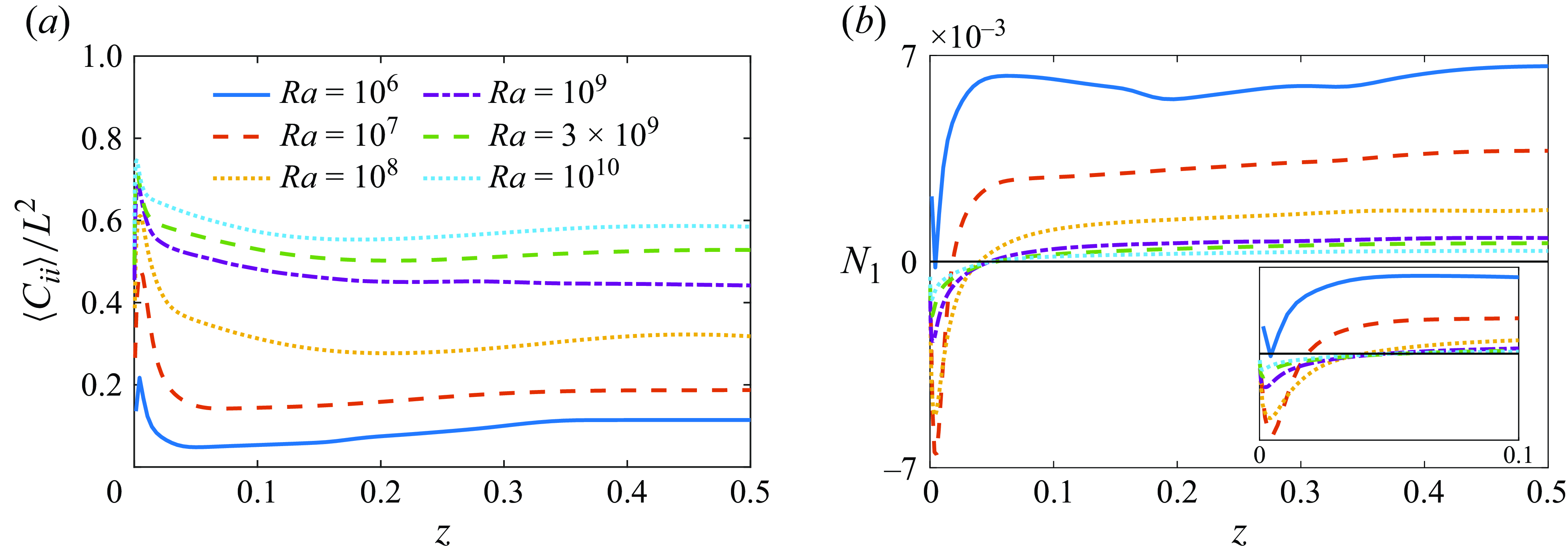
Figure 10. Profiles of (a) mean trace $ \langle C_{ii} \rangle$
normalised by
$ \langle C_{ii} \rangle$
normalised by $L^2$
, and (b) first normal stress difference
$L^2$
, and (b) first normal stress difference $N_1$
of viscoelastic flows at different
$N_1$
of viscoelastic flows at different $Ra$
for
$Ra$
for $Wi=10$
.
$Wi=10$
.
Next, we explore the impact of polymer additives on the deformation of polymer molecules. Figure 10(a) presents wall-normal profiles of the mean trace of the polymer conformation tensor, representing the average polymer length, normalised by the square of the polymer extensibility parameter, $\langle C_{ii} \rangle /L^2$
. The data in the figure reveal that the polymer extension increases with
$\langle C_{ii} \rangle /L^2$
. The data in the figure reveal that the polymer extension increases with $Ra$
, indicating stronger polymer–flow interactions due to the enhanced turbulent intensity. Moreover, as expected, the maximum values of the trace are observed near the wall, whereas in the bulk region, especially far from the wall, the polymer stretching remains relatively uniform. A classic measure of the non-Newtonian character of a suspension is the first normal stress difference, defined as
$Ra$
, indicating stronger polymer–flow interactions due to the enhanced turbulent intensity. Moreover, as expected, the maximum values of the trace are observed near the wall, whereas in the bulk region, especially far from the wall, the polymer stretching remains relatively uniform. A classic measure of the non-Newtonian character of a suspension is the first normal stress difference, defined as $N_1 = (1-\beta )\sqrt {Pr/Ra}(\langle \tau _{zz} \rangle - \langle \tau _{xx}\rangle )$
, the normalised difference between two components of the normal stresses. Note that with our definition of
$N_1 = (1-\beta )\sqrt {Pr/Ra}(\langle \tau _{zz} \rangle - \langle \tau _{xx}\rangle )$
, the normalised difference between two components of the normal stresses. Note that with our definition of $N_1$
, we consider
$N_1$
, we consider $z$
the principal flow direction (which is the case in the bulk but not in the thermal BLs). The wall-normal profiles of
$z$
the principal flow direction (which is the case in the bulk but not in the thermal BLs). The wall-normal profiles of $N_1$
are depicted in figure 10(b). Near the wall,
$N_1$
are depicted in figure 10(b). Near the wall, $N_1$
is negative except for case
$N_1$
is negative except for case $Ra=10^6$
, whereas in the bulk region, it becomes positive, with positive values smaller than the absolute values of the negative ones. This validates the conclusion in Benzi et al. (Reference Benzi, Ching and De Angelis2016b
), who showed that when the stretching of polymers occurs predominantly within the BL, HTR could be observed. Also it implies that near the wall,
$Ra=10^6$
, whereas in the bulk region, it becomes positive, with positive values smaller than the absolute values of the negative ones. This validates the conclusion in Benzi et al. (Reference Benzi, Ching and De Angelis2016b
), who showed that when the stretching of polymers occurs predominantly within the BL, HTR could be observed. Also it implies that near the wall, $\tau _{xx}$
dominates and the polymer undergoes greater stretching in the horizontal direction, while in the bulk,
$\tau _{xx}$
dominates and the polymer undergoes greater stretching in the horizontal direction, while in the bulk, $\tau _{zz}$
dominates and the stretching is more pronounced in the vertical direction. This observation is intuitive, as the polymer chains align with the primary flow direction. Indeed, a positive normal stress difference indicates that polymer chains are becoming oriented in the direction of the flow, in agreement with the visualisations shown above. For the case
$\tau _{zz}$
dominates and the stretching is more pronounced in the vertical direction. This observation is intuitive, as the polymer chains align with the primary flow direction. Indeed, a positive normal stress difference indicates that polymer chains are becoming oriented in the direction of the flow, in agreement with the visualisations shown above. For the case $Ra=10^6$
, the polymer stretching is mainly in the vertical direction, which is expected since the flow is laminar, and the plumes become less wavy with polymers, resulting in reduced horizontal motion. Furthermore, an increase in
$Ra=10^6$
, the polymer stretching is mainly in the vertical direction, which is expected since the flow is laminar, and the plumes become less wavy with polymers, resulting in reduced horizontal motion. Furthermore, an increase in $Ra$
results in a monotonic decrease of the magnitude of
$Ra$
results in a monotonic decrease of the magnitude of $N_1$
. Since the flows become more chaotic and turbulent as
$N_1$
. Since the flows become more chaotic and turbulent as $Ra$
increases, the polymers are not able to maintain significant stretching in one specific direction due to the increasingly isotropic and fluctuating nature of the flow. To conclude, we note that from a dynamics perspective, we therefore retrieve a positive value of
$Ra$
increases, the polymers are not able to maintain significant stretching in one specific direction due to the increasingly isotropic and fluctuating nature of the flow. To conclude, we note that from a dynamics perspective, we therefore retrieve a positive value of $N_1$
for the average flow direction, as typically observed in shear flows. This indicates the presence of elasticity, polymer molecules trying to return to their coiled state.
$N_1$
for the average flow direction, as typically observed in shear flows. This indicates the presence of elasticity, polymer molecules trying to return to their coiled state.
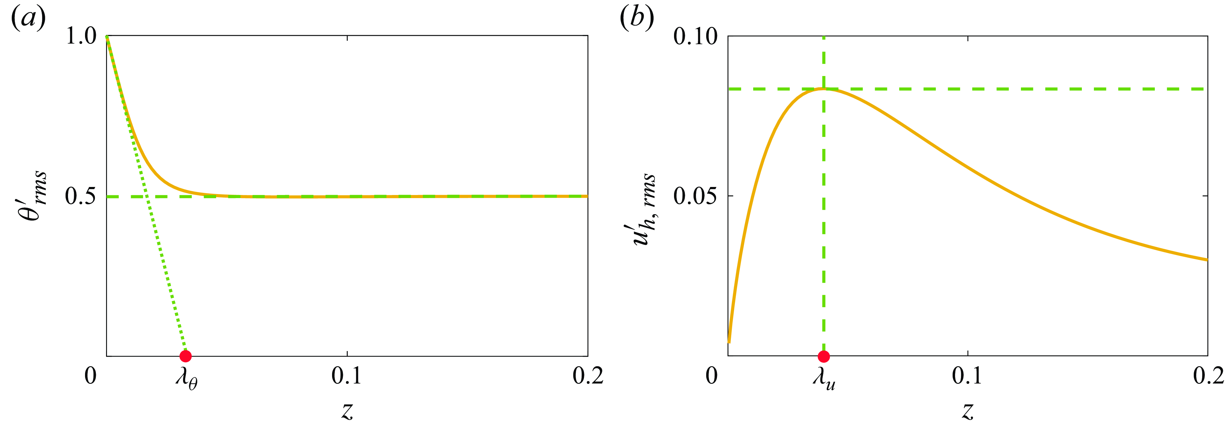
Figure 11. Visualisation of the definitions of (a) thermal and (b) viscous BL thicknesses using the example of the flow for $Ra=10^8$
and
$Ra=10^8$
and $Wi=10$
.
$Wi=10$
.
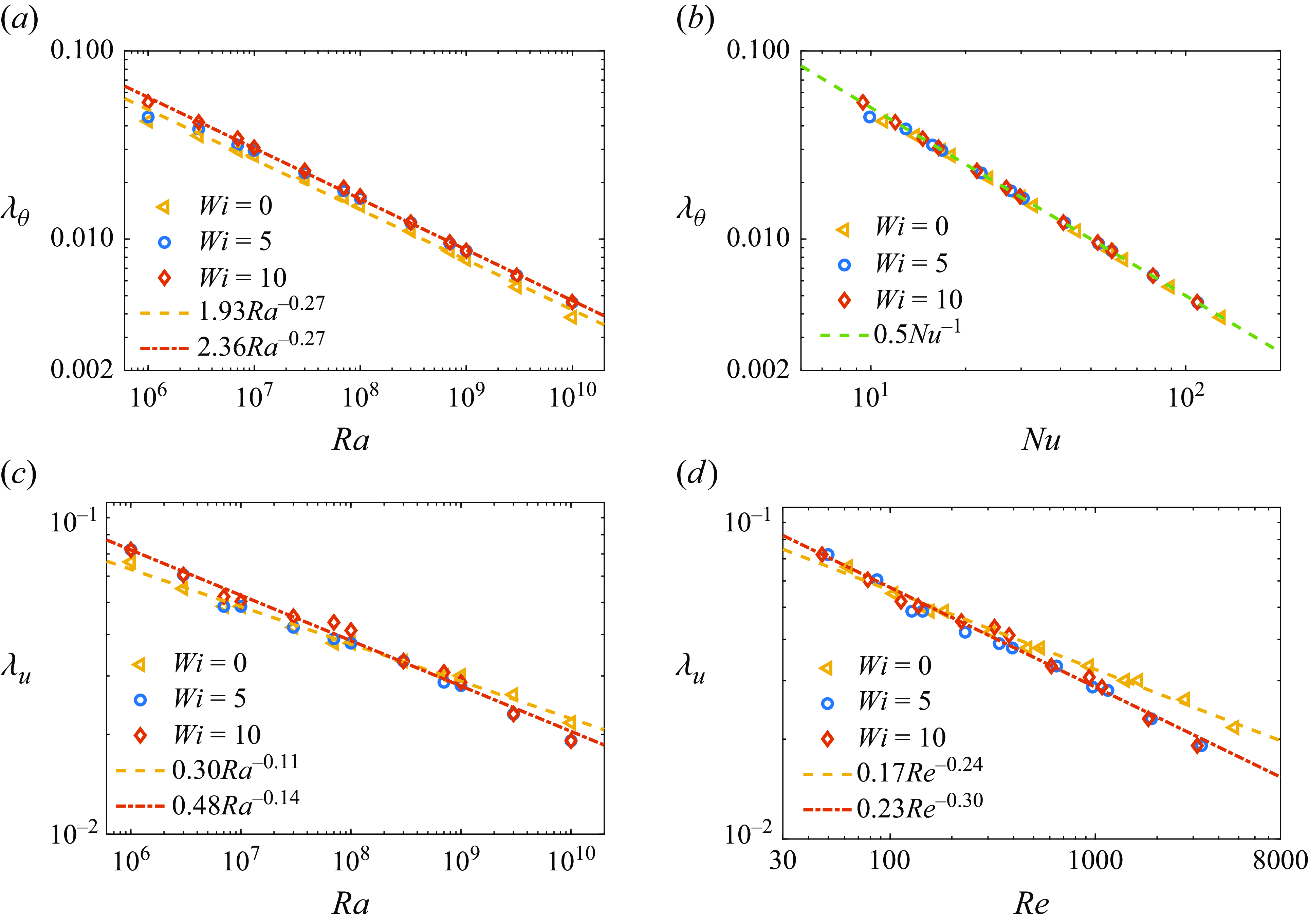
Figure 12. The thermal BL thickness $\lambda _{\theta }$
versus (a) the Rayleigh number
$\lambda _{\theta }$
versus (a) the Rayleigh number $Ra$
and (b) the Nusselt number
$Ra$
and (b) the Nusselt number $Nu$
. The viscous BL thickness
$Nu$
. The viscous BL thickness $\lambda _{u}$
versus (c)
$\lambda _{u}$
versus (c) $Ra$
and (d)
$Ra$
and (d) $Re$
. The dashed lines depict a polynomial fitting to the data. For better visualisation, in (a) and (c) we present only the fitting lines corresponding to
$Re$
. The dashed lines depict a polynomial fitting to the data. For better visualisation, in (a) and (c) we present only the fitting lines corresponding to $Wi=0$
and
$Wi=0$
and $Wi=10$
.
$Wi=10$
.
Next, we investigate the effects of polymer additives on the BL thickness. We adopt the frequently used slope method to define the edge of the thermal BL. That is, the thermal BL is defined as the depth where the linear fit to the mean temperature profile $\theta$
near the bottom (or top) wall intersects the linear fit to the mean temperature profile at mid-height, as illustrated in figure 11(a). The viscous BL, instead, is defined as the distance between the wall and the maximum value of the horizontal velocity fluctuations,
$\theta$
near the bottom (or top) wall intersects the linear fit to the mean temperature profile at mid-height, as illustrated in figure 11(a). The viscous BL, instead, is defined as the distance between the wall and the maximum value of the horizontal velocity fluctuations, $u_{h,{rms}}^{\prime }$
; see figure 11(b). The thermal and viscous BL thicknesses and their scaling behaviours are presented in figure 12. Figure 12(a) shows that the thermal BL thickness increases when adding polymer additives, suggesting an enhanced thermal BL stability. For smaller
$u_{h,{rms}}^{\prime }$
; see figure 11(b). The thermal and viscous BL thicknesses and their scaling behaviours are presented in figure 12. Figure 12(a) shows that the thermal BL thickness increases when adding polymer additives, suggesting an enhanced thermal BL stability. For smaller $Ra$
, this increase is more pronounced with higher
$Ra$
, this increase is more pronounced with higher $Wi=10$
. On the contrary, at larger
$Wi=10$
. On the contrary, at larger $Ra$
, the thermal BL thicknesses remain nearly constant for both
$Ra$
, the thermal BL thicknesses remain nearly constant for both $Wi=5$
and
$Wi=5$
and $Wi=10$
, indicating that the thermal BL thickness becomes less sensitive to polymer extensibility as
$Wi=10$
, indicating that the thermal BL thickness becomes less sensitive to polymer extensibility as $Ra$
increases. However, the polymer additives do not modify the scaling of
$Ra$
increases. However, the polymer additives do not modify the scaling of $\lambda _\theta$
with respect to
$\lambda _\theta$
with respect to $Ra$
. Moreover, all the data collapse on the line
$Ra$
. Moreover, all the data collapse on the line $0.5Nu^{-1}$
(see figure 12
b), fitting well with the theoretical prediction:
$0.5Nu^{-1}$
(see figure 12
b), fitting well with the theoretical prediction: $\lambda _\theta = H/(2Nu)$
for turbulent thermal convection. Interestingly, the viscous BL thickness exhibits a different behaviour. Specifically, the viscous BL thickness scales differently in flows with polymers than in Newtonian flows, displaying a steeper decrease of
$\lambda _\theta = H/(2Nu)$
for turbulent thermal convection. Interestingly, the viscous BL thickness exhibits a different behaviour. Specifically, the viscous BL thickness scales differently in flows with polymers than in Newtonian flows, displaying a steeper decrease of $\lambda _u$
with increasing
$\lambda _u$
with increasing $Ra$
. The intersection of the
$Ra$
. The intersection of the $\lambda _u$
curves in Newtonian and viscoelastic flows happens at approximately
$\lambda _u$
curves in Newtonian and viscoelastic flows happens at approximately $Ra=10^8$
. The scaling of
$Ra=10^8$
. The scaling of $\lambda _u$
with
$\lambda _u$
with $Re$
yields
$Re$
yields $\lambda _u \sim Re^{-0.24}$
for Newtonian flows, as found previously in both simulations (Breuer et al. Reference Breuer, Wessling, Schmalzl and Hansen2004; King, Stellmach & Buffett Reference King, Stellmach and Buffett2013) and experiments (Lam et al. Reference Lam, Shang, Zhou and Xia2002). For the viscoelastic cases, the scaling becomes steeper,
$\lambda _u \sim Re^{-0.24}$
for Newtonian flows, as found previously in both simulations (Breuer et al. Reference Breuer, Wessling, Schmalzl and Hansen2004; King, Stellmach & Buffett Reference King, Stellmach and Buffett2013) and experiments (Lam et al. Reference Lam, Shang, Zhou and Xia2002). For the viscoelastic cases, the scaling becomes steeper, $\lambda _u \sim Re^{-0.30}$
, indicating a modification of the kinetic BL dynamics.
$\lambda _u \sim Re^{-0.30}$
, indicating a modification of the kinetic BL dynamics.
4. Discussion
4.1. Effective viscosity
It is generally argued in the literature that HTR is related to the enhanced stability of the thermal BL, which can be attributed to two primary factors (Xie et al. Reference Xie, Huang, Funfschilling, Li, Ni and Xia2015): (i) the reduced bulk velocity fluctuations that constantly perturb the BL, as depicted in figure 8; (ii) the increased effective viscosity of the polymer solutions that reduces the convection velocity. In order to verify this, we examine the relative effective viscosity of the polymer solutions. According to Benzi et al. (Reference Benzi, Ching and De Angelis2016a
), the relation between the space-dependent effective viscosity $\nu _{\textit {eff}}$
and the solvent viscosity
$\nu _{\textit {eff}}$
and the solvent viscosity $\nu _{s}$
can be expressed as
$\nu _{s}$
can be expressed as
 \begin{equation} \frac {\nu _{\textit {eff}}}{\nu _s}=\frac {E_p}{\varepsilon _u^{[s]}}, \end{equation}
where $E_p$
is the rate of energy transferred to polymer elastic energy, calculated by
$E_p$
is the rate of energy transferred to polymer elastic energy, calculated by $E_p=({1}/{2})({1-\beta }/{Re})\tau _{ii}$
(Min et al. Reference Min, Yoo, Choi and Joseph2003), and
$E_p=({1}/{2})({1-\beta }/{Re})\tau _{ii}$
(Min et al. Reference Min, Yoo, Choi and Joseph2003), and $\varepsilon _u^{[s]}$
is the solvent viscous dissipation rate defined in (2.9).
$\varepsilon _u^{[s]}$
is the solvent viscous dissipation rate defined in (2.9).
Figure 13 depicts the wall-normal profiles of the effective viscosity $\nu _{{eff}}$
normalised by the solvent viscosity
$\nu _{{eff}}$
normalised by the solvent viscosity $\nu _s$
for the polymeric flows. The data show that the normalised effective viscosity exhibits a local maximum in the near-wall region, with a smaller value compared to the bulk region. As one moves away from the wall, the effective viscosity increases (more dramatically at lower
$\nu _s$
for the polymeric flows. The data show that the normalised effective viscosity exhibits a local maximum in the near-wall region, with a smaller value compared to the bulk region. As one moves away from the wall, the effective viscosity increases (more dramatically at lower $Ra$
) and then remains almost constant inside the bulk region. This indicates that the interaction between polymers and the turbulent flow is more pronounced in the bulk, leading to a more pronounced enhancement of viscosity in that region. The non-monotonic behaviour observed near the wall is difficult to explain only from the definition in (4.1) and the complex interactions between turbulence and viscoelastic effects. The local maxima near the wall may be related to the peak of the polymer elastic energy (profiles of
$Ra$
) and then remains almost constant inside the bulk region. This indicates that the interaction between polymers and the turbulent flow is more pronounced in the bulk, leading to a more pronounced enhancement of viscosity in that region. The non-monotonic behaviour observed near the wall is difficult to explain only from the definition in (4.1) and the complex interactions between turbulence and viscoelastic effects. The local maxima near the wall may be related to the peak of the polymer elastic energy (profiles of $E_p$
), and are similar to the trace
$E_p$
), and are similar to the trace $\langle C_{ii}\rangle$
presented in figure 10(a).
$\langle C_{ii}\rangle$
presented in figure 10(a).

Figure 13. Wall-normal profiles of the effective viscosity $\nu _{{eff}}$
normalised by the solvent viscosity
$\nu _{{eff}}$
normalised by the solvent viscosity $\nu _s$
for different values of
$\nu _s$
for different values of $Ra$
.
$Ra$
.
More importantly, we observe that $\nu _{{eff}}$
is correlated with the ratio of Reynolds numbers
$\nu _{{eff}}$
is correlated with the ratio of Reynolds numbers $Re^V/Re^N$
shown in figure 3(d). With increasing
$Re^V/Re^N$
shown in figure 3(d). With increasing $Ra$
, the effective viscosity ratio increases, leading to a decrease in
$Ra$
, the effective viscosity ratio increases, leading to a decrease in $Re$
up to
$Re$
up to $Ra = 10^9$
. Beyond this threshold, the effective viscosity remains nearly unchanged, resulting in an almost constant
$Ra = 10^9$
. Beyond this threshold, the effective viscosity remains nearly unchanged, resulting in an almost constant $Re$
. We then can conclude that for
$Re$
. We then can conclude that for $Ra\lt 10^9$
, the increased viscosity causes a slower circulation, as corroborated by the supplementary movies, thus decreasing the heat transfer rate. Further, the effective viscosity ratios are almost equal for higher
$Ra\lt 10^9$
, the increased viscosity causes a slower circulation, as corroborated by the supplementary movies, thus decreasing the heat transfer rate. Further, the effective viscosity ratios are almost equal for higher $Ra\geqslant 10^9$
, meaning that there may exist a maximum drag enhancement. The additional HTR for
$Ra\geqslant 10^9$
, meaning that there may exist a maximum drag enhancement. The additional HTR for $Ra\gt 10^9$
is therefore caused by other factors, which we discuss below.
$Ra\gt 10^9$
is therefore caused by other factors, which we discuss below.
4.2. Heat flux from plume and turbulence background in the mid-height plane
In this subsection, we aim to investigate why the heat transport is reduced and why the HTR shows a non-monotonic trend with $Ra$
. Since plumes are the primary carrier of heat in turbulent thermal convection, we consider the contribution from the plumes and the turbulent background separately. First, we calculate the probability density functions (PDFs) of the vertical heat flux (
$Ra$
. Since plumes are the primary carrier of heat in turbulent thermal convection, we consider the contribution from the plumes and the turbulent background separately. First, we calculate the probability density functions (PDFs) of the vertical heat flux ( $u_z \theta ^{\prime }$
) at the mid-height plane. It should be noted that
$u_z \theta ^{\prime }$
) at the mid-height plane. It should be noted that $Nu_{centre}=\sqrt {Ra\,Pr}\, \langle u_z\theta ^{\prime }\rangle _{A,t}$
(Kaczorowski & Xia Reference Kaczorowski and Xia2013). The negative part of the vertical heat flux PDF is due to turbulent background fluctuations, known as incoherent heat flux, while the positive part contains both incoherent heat flux and coherent heat flux arising from plumes (Shang et al. Reference Shang, Qiu, Tong and Xia2003; Xie et al. Reference Xie, Huang, Funfschilling, Li, Ni and Xia2015). The large positive value of
$Nu_{centre}=\sqrt {Ra\,Pr}\, \langle u_z\theta ^{\prime }\rangle _{A,t}$
(Kaczorowski & Xia Reference Kaczorowski and Xia2013). The negative part of the vertical heat flux PDF is due to turbulent background fluctuations, known as incoherent heat flux, while the positive part contains both incoherent heat flux and coherent heat flux arising from plumes (Shang et al. Reference Shang, Qiu, Tong and Xia2003; Xie et al. Reference Xie, Huang, Funfschilling, Li, Ni and Xia2015). The large positive value of $u_z \theta ^{\prime }$
should be related to plumes. For each case presented in figure 14, the dataset includes flow field information for at least 300 dimensionless time units. Intriguingly, the PDFs exhibit different characteristics for small
$u_z \theta ^{\prime }$
should be related to plumes. For each case presented in figure 14, the dataset includes flow field information for at least 300 dimensionless time units. Intriguingly, the PDFs exhibit different characteristics for small $Ra$
(
$Ra$
( $Ra \lt 10^9$
) and relatively high
$Ra \lt 10^9$
) and relatively high $Ra$
(
$Ra$
( $Ra \geqslant 10^9$
) regimes.
$Ra \geqslant 10^9$
) regimes.
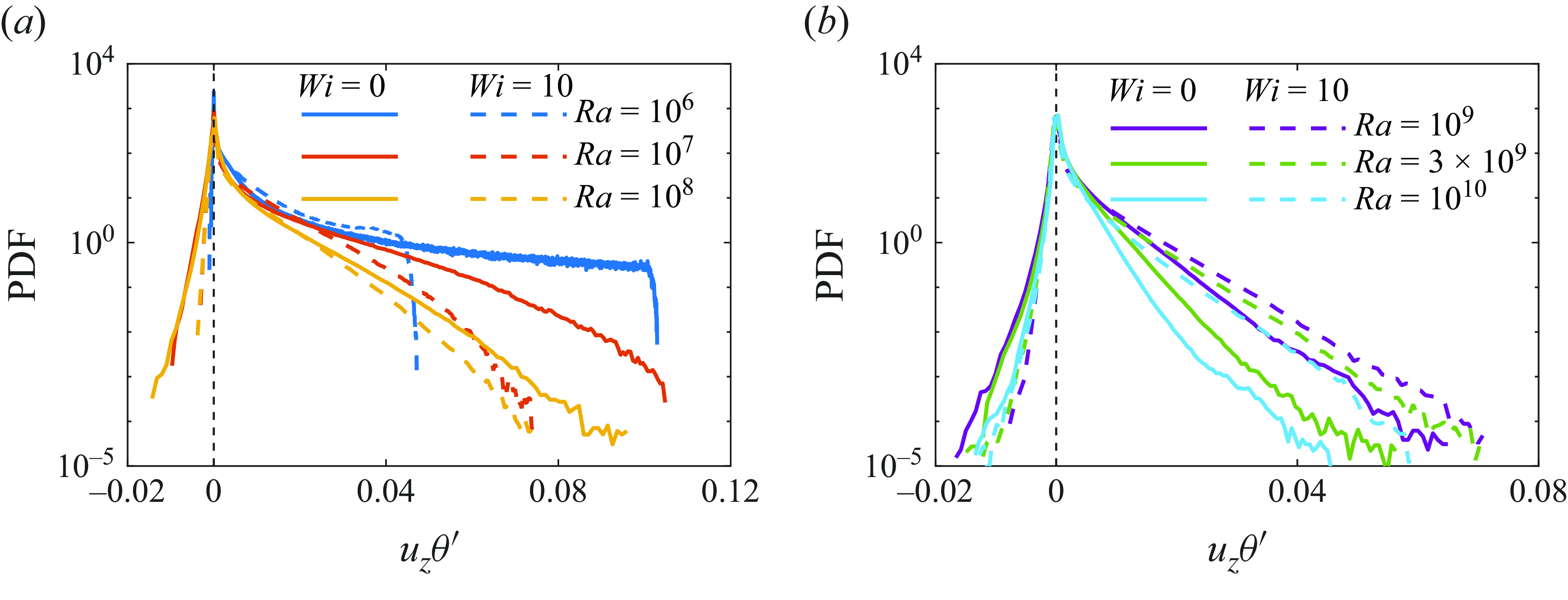
Figure 14. Probability density functions (PDFs) of the vertical heat flux $ u_z \theta ^{\prime }$
at the mid-height plane for (a)
$ u_z \theta ^{\prime }$
at the mid-height plane for (a) $Ra\lt 10^9$
and (b)
$Ra\lt 10^9$
and (b) $Ra\geqslant 10^9$
.
$Ra\geqslant 10^9$
.
In the low $Ra \lt 10^9$
regime, as depicted in figure 14(a), the addition of polymer additives leads to a significant suppression of both negative and positive tails, particularly for very large values of the positive vertical heat flux – those related to the plumes, suggesting a suppression of both incoherent turbulent background fluctuations and coherent heat transport. This effect is more pronounced for smaller
$Ra \lt 10^9$
regime, as depicted in figure 14(a), the addition of polymer additives leads to a significant suppression of both negative and positive tails, particularly for very large values of the positive vertical heat flux – those related to the plumes, suggesting a suppression of both incoherent turbulent background fluctuations and coherent heat transport. This effect is more pronounced for smaller $Ra$
. The suppression of incoherent heat flux is confirmed by the significant decrease in horizontal turbulent fluctuations in the central plane discussed above (see figure 8). This substantial suppression of the coherent flux is attributed to a slower circulation speed, which is more evident for
$Ra$
. The suppression of incoherent heat flux is confirmed by the significant decrease in horizontal turbulent fluctuations in the central plane discussed above (see figure 8). This substantial suppression of the coherent flux is attributed to a slower circulation speed, which is more evident for $Ra=10^6$
, where we observe a pair of convection cells of lower LSC speed (see supplementary movies 1 and 2). Since the relative effective viscosity ratio increases significantly with
$Ra=10^6$
, where we observe a pair of convection cells of lower LSC speed (see supplementary movies 1 and 2). Since the relative effective viscosity ratio increases significantly with $Ra$
, one would intuitively expect a stronger suppression of the coherent motions at higher
$Ra$
, one would intuitively expect a stronger suppression of the coherent motions at higher $Ra$
. However, the figure shows the opposite trend, which may indicate that polymers have a twofold action. For higher
$Ra$
. However, the figure shows the opposite trend, which may indicate that polymers have a twofold action. For higher $Ra\geqslant 10^9$
(see figure 14
b), our observations align with the Xie et al. (Reference Xie, Huang, Funfschilling, Li, Ni and Xia2015) finding that the negative part of the PDF is suppressed, and the probability of large positive values is significantly higher for the polymer solutions. Given the slight increase in temperature fluctuations (see figure 9) and the halving of the velocity fluctuations at mid-height (see figure 8), this enhancement is most likely due to the increased correlation between velocity and temperature, in other words, to the increasing coherence of the thermal plumes. In summary, the data suggest that in the laminar or weakly turbulent regime,
$Ra\geqslant 10^9$
(see figure 14
b), our observations align with the Xie et al. (Reference Xie, Huang, Funfschilling, Li, Ni and Xia2015) finding that the negative part of the PDF is suppressed, and the probability of large positive values is significantly higher for the polymer solutions. Given the slight increase in temperature fluctuations (see figure 9) and the halving of the velocity fluctuations at mid-height (see figure 8), this enhancement is most likely due to the increased correlation between velocity and temperature, in other words, to the increasing coherence of the thermal plumes. In summary, the data suggest that in the laminar or weakly turbulent regime, $Ra \lt 10^9$
, polymers reduce the plume intensity, whereas at larger
$Ra \lt 10^9$
, polymers reduce the plume intensity, whereas at larger $Ra\geqslant 10^9$
, they enhance the coherent transport by the plumes by reducing the effect of the background fluctuations.
$Ra\geqslant 10^9$
, they enhance the coherent transport by the plumes by reducing the effect of the background fluctuations.
To assess more quantitatively the effect of polymers additive on plumes, it is crucial to detect plumes and then separate them from the background fluctuations. In previous studies, various methods have been employed to extract plumes based on their distinct characteristics, such as high temperature (Zhou & Xia Reference Zhou and Xia2002), high thermal dissipation rate (Shishkina & Wagner Reference Shishkina and Wagner2006, Reference Shishkina and Wagner2008), high vertical heat flux (Ching et al. Reference Ching, Guo, Shang, Tong and Xia2004), and negative horizontal divergence of the horizontal velocity field (Shevkar et al. Reference Shevkar, Vishnu, Mohanan, Koothur, Mathur and Puthenveettil2022). Here, we adopt the criteria that combine both temperature and heat flux conditions (Huang et al. Reference Huang, Kaczorowski, Ni and Xia2013; van der Poel et al. Reference van der Poel, Verzicco, Grossmann and Lohse2015a
). That is, in a certain horizontal cross-section, the plume is the area satisfying $\pm [\theta (x,y)-\langle \theta \rangle _{xy}] \gt c \langle \theta _{{rms}}\rangle _{xy}$
and
$\pm [\theta (x,y)-\langle \theta \rangle _{xy}] \gt c \langle \theta _{{rms}}\rangle _{xy}$
and $\sqrt {Ra\, Pr}\,u_z(x,y)\,\theta ^{\prime }(x,y) \gt c (Nu-1)$
, where ‘
$\sqrt {Ra\, Pr}\,u_z(x,y)\,\theta ^{\prime }(x,y) \gt c (Nu-1)$
, where ‘ $+$
’ indicates a hot plume, and ‘
$+$
’ indicates a hot plume, and ‘ $-$
’ indicates a cold one.
$-$
’ indicates a cold one.
Note that we use the factor $(Nu-1)$
to exclude conductive heat transfer. The remaining part of the cross-section is defined as background. We choose the same empirical constant
$(Nu-1)$
to exclude conductive heat transfer. The remaining part of the cross-section is defined as background. We choose the same empirical constant $c=1.2$
as in van der Poel et al. (Reference van der Poel, Verzicco, Grossmann and Lohse2015a
). The choice of
$c=1.2$
as in van der Poel et al. (Reference van der Poel, Verzicco, Grossmann and Lohse2015a
). The choice of $c$
influences the absolute value of the plume area and plume mean velocity, but the trends presented below remain independent of
$c$
influences the absolute value of the plume area and plume mean velocity, but the trends presented below remain independent of $c$
. The results of this plume-extraction procedure are displayed in figure 15 for both Newtonian and viscoelastic flows at
$c$
. The results of this plume-extraction procedure are displayed in figure 15 for both Newtonian and viscoelastic flows at $Ra=10^8$
. One can see that this criterion successfully extracts both hot and cold plumes in the thermal BL and bulk regions. We use this procedure to calculate the mean temperature and vertical velocity of plumes, as well as the heat flux contributions from both plumes and background, in the middle-height plane by averaging over 300 free-fall time units.
$Ra=10^8$
. One can see that this criterion successfully extracts both hot and cold plumes in the thermal BL and bulk regions. We use this procedure to calculate the mean temperature and vertical velocity of plumes, as well as the heat flux contributions from both plumes and background, in the middle-height plane by averaging over 300 free-fall time units.
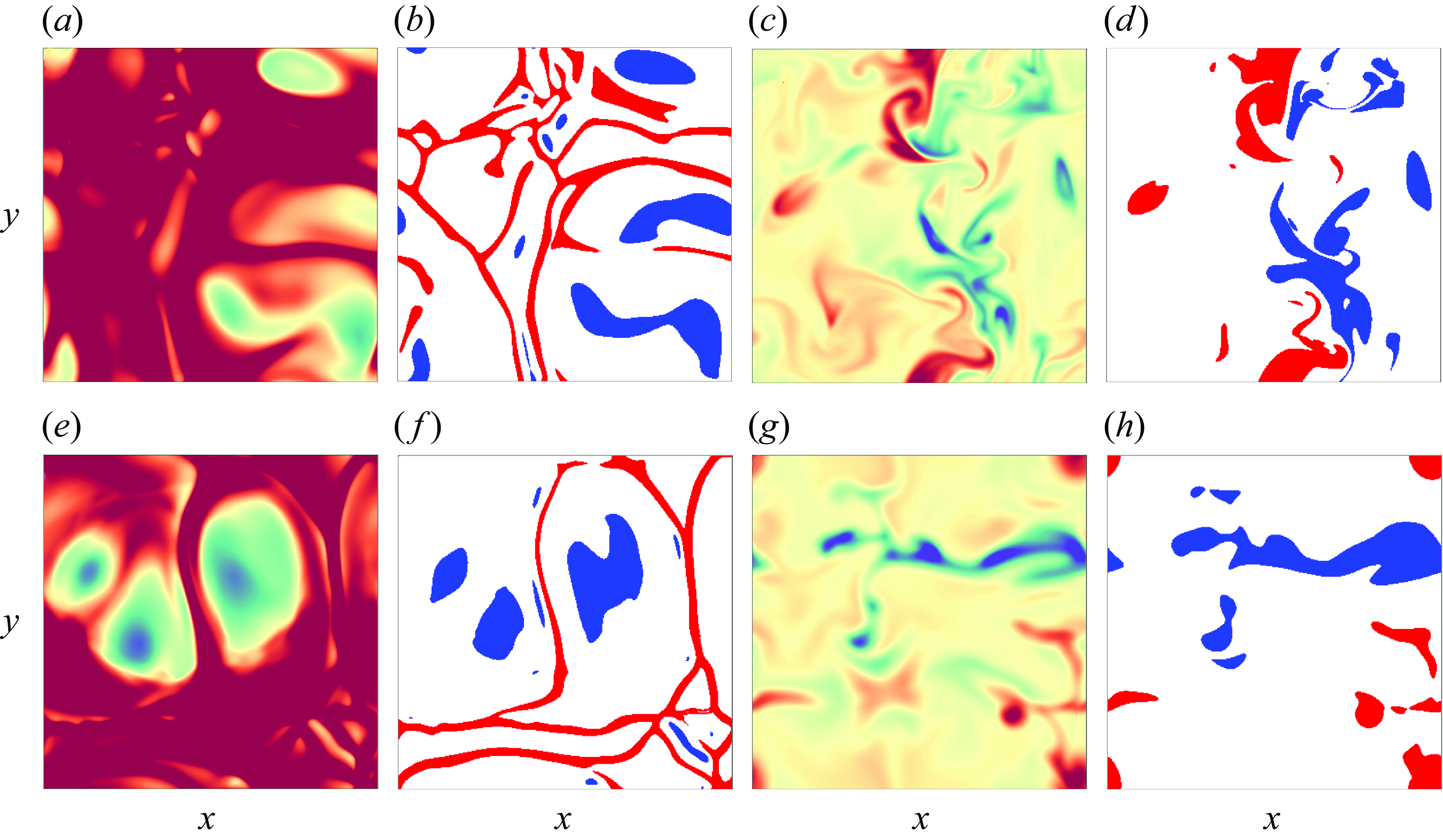
Figure 15. Plumes extraction at (a,b,e,f) the edge of the thermal BL ( $z=0.5H/Nu$
) and (c,d,g,h) the middle-height
$z=0.5H/Nu$
) and (c,d,g,h) the middle-height $xy$
-plane for (a,b,c,d) Newtonian and (e,f,g,h) viscoelastic (
$xy$
-plane for (a,b,c,d) Newtonian and (e,f,g,h) viscoelastic ( $Wi=10$
) flows at
$Wi=10$
) flows at $Ra=10^8,\ Pr=4.3$
. The temperature shown in (a,c,e,g) has the same colour bar as in figure 6, and the red and blue colours in (b,d,f,h) denote the extracted hot and cold plumes, respectively.
$Ra=10^8,\ Pr=4.3$
. The temperature shown in (a,c,e,g) has the same colour bar as in figure 6, and the red and blue colours in (b,d,f,h) denote the extracted hot and cold plumes, respectively.
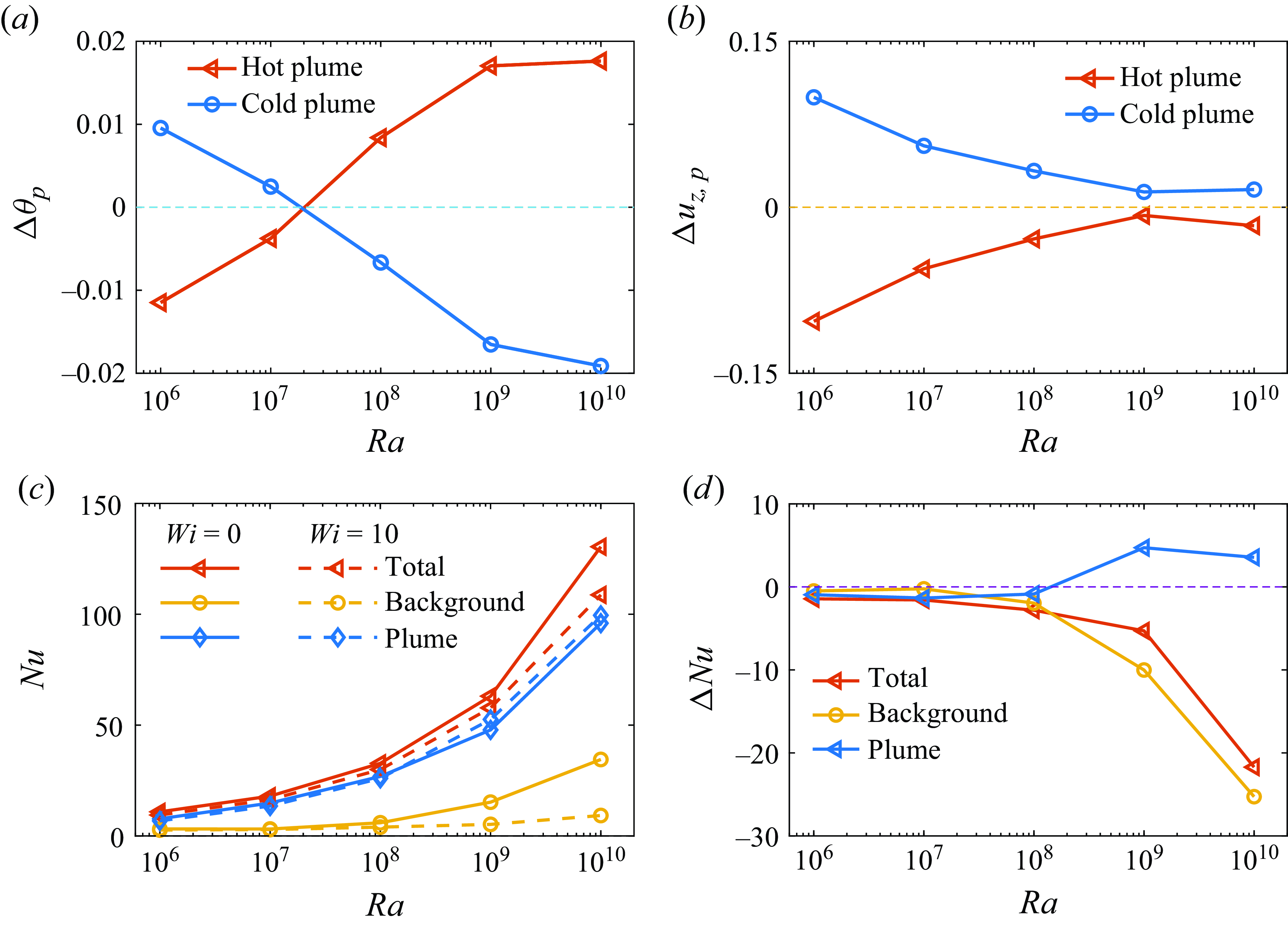
Figure 16. Results of plume extraction: difference in (a) plume mean temperature $\Delta \theta _p = \langle \theta \rangle _{p,t}^V- \langle \theta \rangle _{p,t}^N$
and (b) plume vertical velocity
$\Delta \theta _p = \langle \theta \rangle _{p,t}^V- \langle \theta \rangle _{p,t}^N$
and (b) plume vertical velocity $\Delta u_{z,p} = \langle u_z\rangle _{p,t}^V-\langle u_z\rangle _{p,t}^N$
between Newtonian flows and viscoelastic flows at
$\Delta u_{z,p} = \langle u_z\rangle _{p,t}^V-\langle u_z\rangle _{p,t}^N$
between Newtonian flows and viscoelastic flows at $Wi=10$
. (c) Contributions to the total
$Wi=10$
. (c) Contributions to the total $Nu$
from the plumes and background chaotic flow. (d) Difference
$Nu$
from the plumes and background chaotic flow. (d) Difference $\Delta Nu= Nu^V-Nu^N$
between Newtonian and viscoelastic flows at
$\Delta Nu= Nu^V-Nu^N$
between Newtonian and viscoelastic flows at $Wi=10$
, considering the heat flux in plumes, background, and the total value.
$Wi=10$
, considering the heat flux in plumes, background, and the total value.
Figure 16(a,b) show the mean temperature and mean vertical velocity differences between viscoelastic and Newtonian flows for hot and cold plumes. These are defined as $\Delta \theta _p = \langle \theta \rangle _{p,t}^V- \langle \theta \rangle _{p,t}^N$
and
$\Delta \theta _p = \langle \theta \rangle _{p,t}^V- \langle \theta \rangle _{p,t}^N$
and $\Delta u_{z,p} = \langle u_z\rangle _{p,t}^V-\langle u_z\rangle _{p,t}^N$
. Interestingly, we observe that, compared to the Newtonian flow, the hot plumes are less hot, and the cold plumes are less cold, in viscoelastic flows at small
$\Delta u_{z,p} = \langle u_z\rangle _{p,t}^V-\langle u_z\rangle _{p,t}^N$
. Interestingly, we observe that, compared to the Newtonian flow, the hot plumes are less hot, and the cold plumes are less cold, in viscoelastic flows at small $Ra\lt 10^8$
. However, for
$Ra\lt 10^8$
. However, for $Ra\geqslant 10^8$
, this trend reverses, with hot plumes becoming hotter, and cold plumes becoming colder. Moreover, the magnitude of this difference increases with
$Ra\geqslant 10^8$
, this trend reverses, with hot plumes becoming hotter, and cold plumes becoming colder. Moreover, the magnitude of this difference increases with $Ra$
. The vertical velocity of the plumes in viscoelastic flows is lower than in Newtonian flows, and the magnitude of this decrease becomes smaller with increasing
$Ra$
. The vertical velocity of the plumes in viscoelastic flows is lower than in Newtonian flows, and the magnitude of this decrease becomes smaller with increasing $Ra$
until
$Ra$
until $Ra=10^9$
, beyond which it reaches a plateau, which aligns with the trend for
$Ra=10^9$
, beyond which it reaches a plateau, which aligns with the trend for $Re$
shown in figure 3, and the effective viscosity shown in figure 13. The data seem to confirm our interpretation above: at small
$Re$
shown in figure 3, and the effective viscosity shown in figure 13. The data seem to confirm our interpretation above: at small $Ra$
, the addition of polymers dampens the intensity of thermal plumes by increasing the effective viscosity of the flow. Consequently, the effective thermal diffusivity increases, which leads to a decreased temperature of the hot plumes, and increased temperature of the cold ones. Conversely, at high
$Ra$
, the addition of polymers dampens the intensity of thermal plumes by increasing the effective viscosity of the flow. Consequently, the effective thermal diffusivity increases, which leads to a decreased temperature of the hot plumes, and increased temperature of the cold ones. Conversely, at high $Ra$
, the stabilised BL in the viscoelastic flows makes the released plumes more coherent. Additionally, the presence of polymer additives reduces the turbulence intensity, leading to weaker mixing. This reduced mixing slows down the horizontal heat transport, causing heat to remain more concentrated inside the plumes.
$Ra$
, the stabilised BL in the viscoelastic flows makes the released plumes more coherent. Additionally, the presence of polymer additives reduces the turbulence intensity, leading to weaker mixing. This reduced mixing slows down the horizontal heat transport, causing heat to remain more concentrated inside the plumes.
To further investigate the heat transfer mechanisms, we now discuss the heat flux contributions from the plumes and the background chaotic flow, still focusing on the mid-plane. Figure 16(c) displays the total $Nu=\sqrt {Ra\,Pr}\,\langle u_z \theta ^{\prime }\rangle$
, as well as the heat flux from the turbulent background and plumes. We note that the heat flux from both turbulent background and plumes increases with increasing
$Nu=\sqrt {Ra\,Pr}\,\langle u_z \theta ^{\prime }\rangle$
, as well as the heat flux from the turbulent background and plumes. We note that the heat flux from both turbulent background and plumes increases with increasing $Ra$
, and plumes serve as the main heat carriers for both Newtonian and viscoelastic flows. Focusing on the differences, figure 16(d) presents the HTM between viscoelastic and Newtonian flows
$Ra$
, and plumes serve as the main heat carriers for both Newtonian and viscoelastic flows. Focusing on the differences, figure 16(d) presents the HTM between viscoelastic and Newtonian flows $\Delta Nu = Nu^V-Nu^N$
, considering the total flux, and the plume and background contributions. First, we observe that the heat flux reduction increases with the Rayleigh number, and that this difference can be ascribed to the plumes for
$\Delta Nu = Nu^V-Nu^N$
, considering the total flux, and the plume and background contributions. First, we observe that the heat flux reduction increases with the Rayleigh number, and that this difference can be ascribed to the plumes for $Ra \lesssim 10^7$
, when the flow is in a laminar-like regime. Further increasing
$Ra \lesssim 10^7$
, when the flow is in a laminar-like regime. Further increasing $Ra$
, instead, the reduction is mainly due to the reduction of the background turbulence. The contributions from the plumes actually increase at the largest values of the Rayleigh number under consideration. Nevertheless, the increased heat flux associated with more coherent plumes is not enough to balance the reduction associated with the background fluctuations.
$Ra$
, instead, the reduction is mainly due to the reduction of the background turbulence. The contributions from the plumes actually increase at the largest values of the Rayleigh number under consideration. Nevertheless, the increased heat flux associated with more coherent plumes is not enough to balance the reduction associated with the background fluctuations.
The results therefore confirm the observations made when examining the PDFs. That is, the heat flux in the mid-plane from the background generally decreases with polymer additives, while the heat flux from the plumes first decreases for $Ra\lt 10^9$
, and then increases. While at small
$Ra\lt 10^9$
, and then increases. While at small $Ra$
the reduction in the total heat flux arises mainly from the plumes, at large
$Ra$
the reduction in the total heat flux arises mainly from the plumes, at large $Ra$
, even though the heat flux from the plumes region increases, the significant decrease in the heat flux from the turbulent background determines the total HTR.
$Ra$
, even though the heat flux from the plumes region increases, the significant decrease in the heat flux from the turbulent background determines the total HTR.
Overall, the polymer additives affect the turbulent background and plumes in different ways. That is, polymers act to suppress turbulence in the background flow, leading to lower turbulence intensity. As concerns the plumes, the net effect of polymer additives varies with the Rayleigh number: (i) they reduce the vertical velocity of strong plumes, thereby leading to the suppression of strong heat transport events, and this effect is more pronounced at lower $Ra$
when the background flow is laminar-like; (ii) they enhance the coherence of the plumes, thus increasing the heat flux. These two effects are in competition, with the latter becoming dominant as
$Ra$
when the background flow is laminar-like; (ii) they enhance the coherence of the plumes, thus increasing the heat flux. These two effects are in competition, with the latter becoming dominant as $Ra$
increases. In the following, we investigate how the flow in the BL is affected by the polymers, and how this reflects in the heat fluxes.
$Ra$
increases. In the following, we investigate how the flow in the BL is affected by the polymers, and how this reflects in the heat fluxes.
4.3. Volume-averaged heat flux from plumes, BLs and background
To further elucidate the impact of viscoelasticity on the HTM of the entire system, we examine the contributions of the BLs, plumes and turbulent background to the volume-averaged heat flux derived by the exact relation between $Nu$
and the thermal dissipation rate. The decomposition is based on the criterion for plume extraction, as mentioned previously. The BLs are defined as the regions within distance
$Nu$
and the thermal dissipation rate. The decomposition is based on the criterion for plume extraction, as mentioned previously. The BLs are defined as the regions within distance $0.5H/Nu$
from the top and bottom walls exclusion plume region. The remaining area is classified as turbulent background. Figure 17 displays the differences between the Nusselt numbers of Newtonian and viscoelastic flows across these regions, with all results averaged over 100 free-fall time units. We observe that the total
$0.5H/Nu$
from the top and bottom walls exclusion plume region. The remaining area is classified as turbulent background. Figure 17 displays the differences between the Nusselt numbers of Newtonian and viscoelastic flows across these regions, with all results averaged over 100 free-fall time units. We observe that the total $ \Delta Nu$
shows a non-monotonic trend as the HTR; also, the heat flux contributions from the plumes and background follow trends similar to those observed in the mid-plane, i.e. the total heat transferred by the plumes first decrease and then increase with
$ \Delta Nu$
shows a non-monotonic trend as the HTR; also, the heat flux contributions from the plumes and background follow trends similar to those observed in the mid-plane, i.e. the total heat transferred by the plumes first decrease and then increase with $Ra$
in the viscoelastic flows while it decreases in the background flow, with the latter decrease being more pronounced. Most interestingly, we note that the largest part of the reduction in viscoelastic flows is associated with the heat flux in the BLs, and it increases with
$Ra$
in the viscoelastic flows while it decreases in the background flow, with the latter decrease being more pronounced. Most interestingly, we note that the largest part of the reduction in viscoelastic flows is associated with the heat flux in the BLs, and it increases with $Ra$
. In the experiments by Xie et al. (Reference Xie, Huang, Funfschilling, Li, Ni and Xia2015) at similar
$Ra$
. In the experiments by Xie et al. (Reference Xie, Huang, Funfschilling, Li, Ni and Xia2015) at similar $Ra = 6.18 \times 10^9,\ Pr = 4.3$
, it was found that polymer additives enhance heat transport in the turbulent thermal convection bulk flow by increasing the coherency of thermal plumes and suppressing turbulent background fluctuations. On the other hand, the polymer additives stabilise the thermal BLs and reduce plume release. Xie et al. (Reference Xie, Huang, Funfschilling, Li, Ni and Xia2015) explained the observed HTE in their experiments by saying that the effect of enhanced plume coherency overcomes the effect of reduced plume emission. Their observations on the effects of polymers are consistent with our study. The qualitative difference in heat transport modification – i.e. HTE in their experiments and HTR in our simulations – is attributed to rough walls in their experiments, which makes both kinetic energy and thermal dissipation rates bulk-dominated.
$Ra = 6.18 \times 10^9,\ Pr = 4.3$
, it was found that polymer additives enhance heat transport in the turbulent thermal convection bulk flow by increasing the coherency of thermal plumes and suppressing turbulent background fluctuations. On the other hand, the polymer additives stabilise the thermal BLs and reduce plume release. Xie et al. (Reference Xie, Huang, Funfschilling, Li, Ni and Xia2015) explained the observed HTE in their experiments by saying that the effect of enhanced plume coherency overcomes the effect of reduced plume emission. Their observations on the effects of polymers are consistent with our study. The qualitative difference in heat transport modification – i.e. HTE in their experiments and HTR in our simulations – is attributed to rough walls in their experiments, which makes both kinetic energy and thermal dissipation rates bulk-dominated.
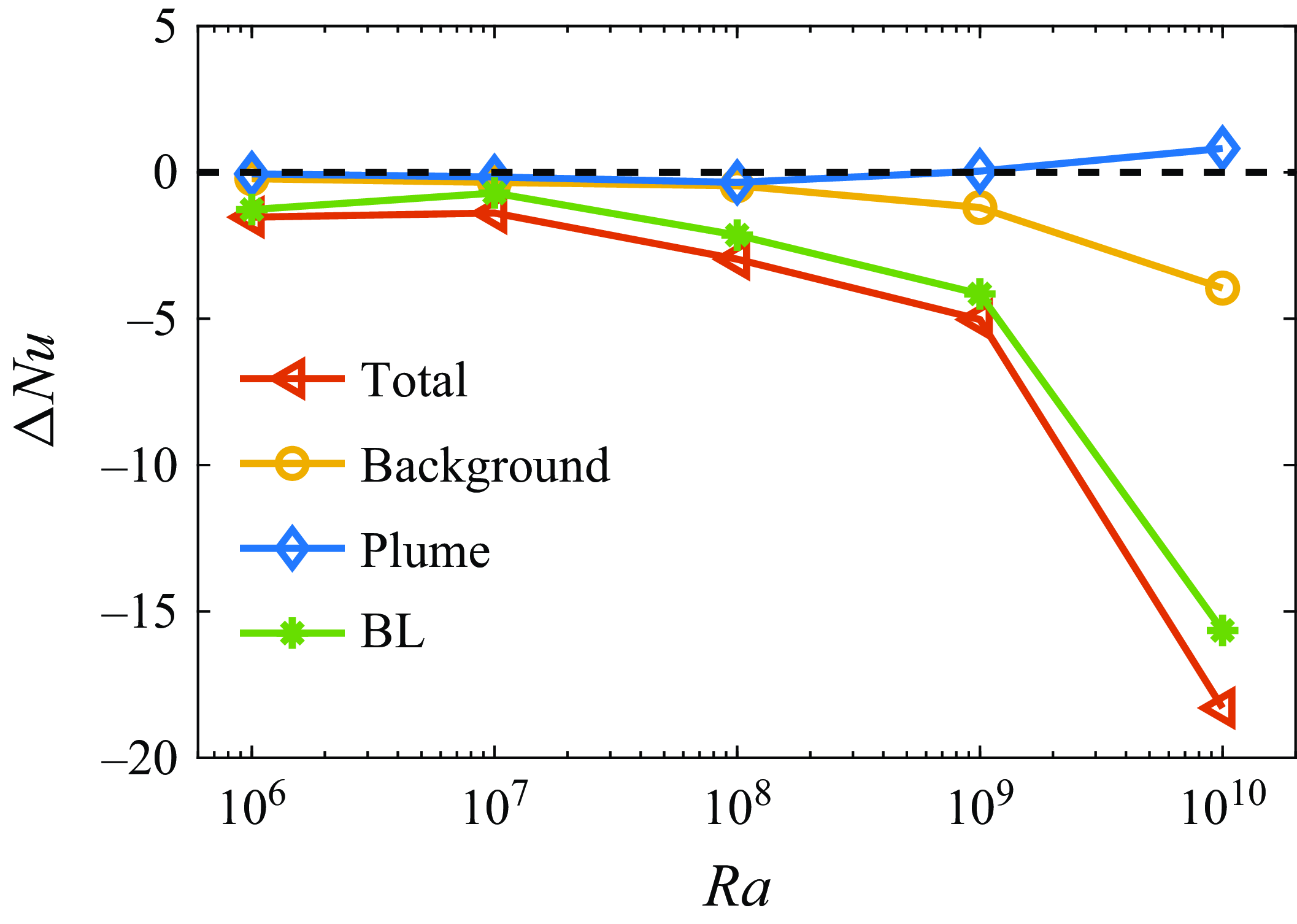
Figure 17. Difference between the Nusselt numbers of Newtonian and viscoelastic flows, $\Delta Nu=Nu^V-Nu^N$
, in different regions: BLs, plumes and background.
$\Delta Nu=Nu^V-Nu^N$
, in different regions: BLs, plumes and background.
4.4. Kinetic energy dissipation rate and energy spectra
In this subsection, we focus on the contribution from turbulence and polymers to the kinetic energy dissipation rate. In viscoelastic flows, the fluid kinetic energy is partly dissipated by the viscous stresses at small scales, and partly transferred to the polymers, which is called the elastic dissipation rate. By taking the dot product of the momentum equation (2.2) with the velocity $u_i$
, and averaging over time and over the entire volume (Benzi et al. Reference Benzi, Ching and De Angelis2016a
), the exact balance between energy production rate by buoyancy, viscous dissipation rate in the Newtonian solvent
$u_i$
, and averaging over time and over the entire volume (Benzi et al. Reference Benzi, Ching and De Angelis2016a
), the exact balance between energy production rate by buoyancy, viscous dissipation rate in the Newtonian solvent $\varepsilon _u^{[s]}$
and elastic dissipation rate due to the polymer additives
$\varepsilon _u^{[s]}$
and elastic dissipation rate due to the polymer additives $\varepsilon _u^{[p]}$
is given as
$\varepsilon _u^{[p]}$
is given as
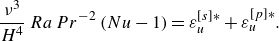 \begin{equation} \frac {\nu ^3}{H^4}\,Ra\,Pr^{-2}\,(Nu-1)=\varepsilon _u^{[s]*}+\varepsilon _u^{[p]*}. \end{equation}
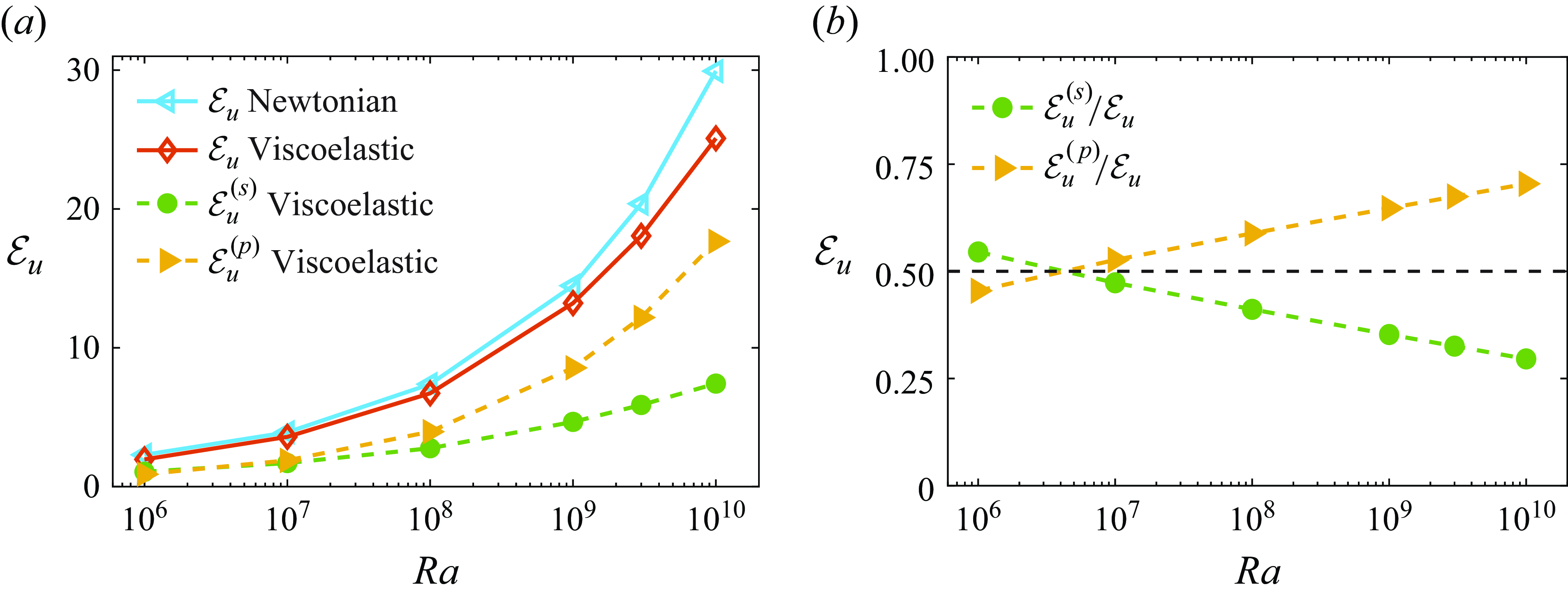
Figure 18. (a) Viscous (circle) and elastic (triangle) energy dissipation rates in Newtonian and viscoelastic ( $Wi=10$
) flows versus
$Wi=10$
) flows versus $Ra$
. (b) The fraction of viscous (green circle) and elastic (yellow triangle) contributions to the total kinetic dissipation rate in viscoelastic flows.
$Ra$
. (b) The fraction of viscous (green circle) and elastic (yellow triangle) contributions to the total kinetic dissipation rate in viscoelastic flows.
After normalisation using $U_{ff}$
and
$U_{ff}$
and $H$
, this can be rewritten as
$H$
, this can be rewritten as
 \begin{equation} \frac {Nu-1}{\sqrt {Ra\,Pr}}=\varepsilon _u^{[s]}+\varepsilon _u^{[p]}= \beta \sqrt {\frac {Pr}{Ra}}\,[\langle \partial _i u_j(\boldsymbol{x},t)\rangle _{V,t}]^2 -(1-\beta )\sqrt {\frac {Pr}{Ra}}\,\langle u_i\,\partial _j \tau _{ij}\rangle _{V,t}. \end{equation}
The value of $Nu$
can thus be directly related to
$Nu$
can thus be directly related to $\varepsilon _u^{[s]}$
and
$\varepsilon _u^{[s]}$
and $\varepsilon _u^{[p]}$
.
$\varepsilon _u^{[p]}$
.
The dissipation rates $\varepsilon _u^{[s]}$
,
$\varepsilon _u^{[s]}$
, $\varepsilon _u^{[p]}$
and total dissipation rate are displayed in figure 18(a). As expected, both
$\varepsilon _u^{[p]}$
and total dissipation rate are displayed in figure 18(a). As expected, both $\varepsilon _u^{[s]}$
and
$\varepsilon _u^{[s]}$
and $\varepsilon _u^{[p]}$
increase with
$\varepsilon _u^{[p]}$
increase with $Ra$
, and the total energy dissipation rates
$Ra$
, and the total energy dissipation rates $\varepsilon _u=\varepsilon _u^{[s]}+\varepsilon _u^{[p]}$
of polymer solutions decrease compared to Newtonian flows, leading to the HTR. Here, the increasing
$\varepsilon _u=\varepsilon _u^{[s]}+\varepsilon _u^{[p]}$
of polymer solutions decrease compared to Newtonian flows, leading to the HTR. Here, the increasing $\varepsilon _u^{[p]}$
is related to the amount of the polymer stretching, as indicated by the trace shown in figure 10(a).
$\varepsilon _u^{[p]}$
is related to the amount of the polymer stretching, as indicated by the trace shown in figure 10(a).
The relative contributions of the viscous and elastic dissipation to the total energy dissipation rate of polymer solutions are reported in figure 18(b). The data in the figure reveal that when increasing $Ra$
, the contribution of the elastic part increases monotonically and becomes dominant over the viscous dissipation at
$Ra$
, the contribution of the elastic part increases monotonically and becomes dominant over the viscous dissipation at $Ra\geqslant 10^7$
, which indicates the growing importance of elastic stresses in the flow. In addition, at higher
$Ra\geqslant 10^7$
, which indicates the growing importance of elastic stresses in the flow. In addition, at higher $Ra$
, more of the kinetic energy is transferred into elastic potential energy as the polymers are stretched by the turbulent flow. This elastic energy is released back to the flow once the polymer stretching reduces. The effect of this mechanism in thermal convection, and how the kinetic energy redistributes at different spatial scales, deserve further investigation.
$Ra$
, more of the kinetic energy is transferred into elastic potential energy as the polymers are stretched by the turbulent flow. This elastic energy is released back to the flow once the polymer stretching reduces. The effect of this mechanism in thermal convection, and how the kinetic energy redistributes at different spatial scales, deserve further investigation.
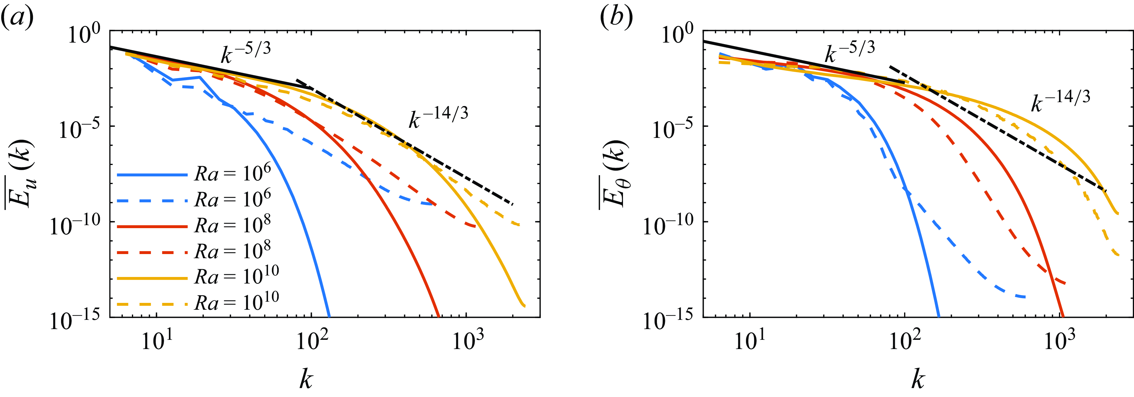
Figure 19 (a) Turbulent kinetic energy spectra normalised by $u_i^2/2$
,
$u_i^2/2$
, $\overline {E_{u}}(k)$
, and (b) temperature energy spectra normalised by
$\overline {E_{u}}(k)$
, and (b) temperature energy spectra normalised by $\theta ^2/2$
,
$\theta ^2/2$
, $\overline {E_{\theta }}(k)$
, sampled at the mid-height of the domain, and averaged over the plane and over time. The spectra are plotted as functions of normalised wavenumber
$\overline {E_{\theta }}(k)$
, sampled at the mid-height of the domain, and averaged over the plane and over time. The spectra are plotted as functions of normalised wavenumber $k$
for different
$k$
for different $Ra$
, comparing Newtonian flows (solid lines) with viscoelastic flows at
$Ra$
, comparing Newtonian flows (solid lines) with viscoelastic flows at $Wi=10$
(dashed lines). The solid and dashed black lines show the scaling laws
$Wi=10$
(dashed lines). The solid and dashed black lines show the scaling laws $-5/3$
and
$-5/3$
and $-14/3$
, respectively.
$-14/3$
, respectively.
To shed some light on these energy transfer mechanisms, we consider the one-dimensional turbulent kinetic energy $\overline {E_{u}}(k)$
and temperature energy spectra
$\overline {E_{u}}(k)$
and temperature energy spectra $\overline {E_{\theta }}(k)$
. The one-dimensional energy spectra are calculated by the fluctuations from the three velocity components and temperature at the middle-height plane. The spectra in figure 19 are obtained by first computing the Fourier transform in the
$\overline {E_{\theta }}(k)$
. The one-dimensional energy spectra are calculated by the fluctuations from the three velocity components and temperature at the middle-height plane. The spectra in figure 19 are obtained by first computing the Fourier transform in the $x$
(or
$x$
(or $y$
) direction, then averaging in the orthogonal horizontal direction, i.e.
$y$
) direction, then averaging in the orthogonal horizontal direction, i.e. $y$
(or
$y$
(or $x$
). Finally, averages are performed over the two horizontal directions and over at least 300 dimensionless time units. As depicted in figure 19(a), with increasing
$x$
). Finally, averages are performed over the two horizontal directions and over at least 300 dimensionless time units. As depicted in figure 19(a), with increasing $Ra$
, the classical inertial scaling
$Ra$
, the classical inertial scaling $k^{-5/3}$
is gradually reached in the Newtonian flows in the intermediate wavenumber range. When polymer additives are added, the large-scale content decreases (energy in the low wavenumber range), while the small-scale energy content increases (high wavenumber range). Moreover, the spectra tend to follow the power-law decay with exponent nearly
$k^{-5/3}$
is gradually reached in the Newtonian flows in the intermediate wavenumber range. When polymer additives are added, the large-scale content decreases (energy in the low wavenumber range), while the small-scale energy content increases (high wavenumber range). Moreover, the spectra tend to follow the power-law decay with exponent nearly $-14/3$
at high
$-14/3$
at high $Ra\geqslant 10^8$
, as also reported in other flow configurations with elasto-inertial turbulence (Dubief et al. Reference Dubief, Terrapon and Soria2013; Sid et al. Reference Sid, Terrapon and Dubief2018; Song et al. Reference Song, Lin, Liu, Lu and Khomami2021). The suppression of large-scale motions and the activation of small-scale fluctuations observed here may be related to polymer stretching (see enhanced polymer dissipation in figure 18), and is consistent with the typical features of elasto-inertial turbulence, where the small-scale motions are sustained by a significant polymer stretching (Sid et al. Reference Sid, Terrapon and Dubief2018). Note that a similar activation of small-scale motions is also observed in other multiphase systems, for example, in emulsions, where the small-scale motions are induced by surface tension releasing energy to the flow upon relaxation and coalescence (Crialesi-Esposito, Chibbaro & Brandt Reference Crialesi-Esposito, Chibbaro and Brandt2023; Moradi Bilondi et al. Reference Moradi Bilondi, Scapin, Brandt and Mirbod2024).
$Ra\geqslant 10^8$
, as also reported in other flow configurations with elasto-inertial turbulence (Dubief et al. Reference Dubief, Terrapon and Soria2013; Sid et al. Reference Sid, Terrapon and Dubief2018; Song et al. Reference Song, Lin, Liu, Lu and Khomami2021). The suppression of large-scale motions and the activation of small-scale fluctuations observed here may be related to polymer stretching (see enhanced polymer dissipation in figure 18), and is consistent with the typical features of elasto-inertial turbulence, where the small-scale motions are sustained by a significant polymer stretching (Sid et al. Reference Sid, Terrapon and Dubief2018). Note that a similar activation of small-scale motions is also observed in other multiphase systems, for example, in emulsions, where the small-scale motions are induced by surface tension releasing energy to the flow upon relaxation and coalescence (Crialesi-Esposito, Chibbaro & Brandt Reference Crialesi-Esposito, Chibbaro and Brandt2023; Moradi Bilondi et al. Reference Moradi Bilondi, Scapin, Brandt and Mirbod2024).
Finally, examining the temperature fluctuation spectra of polymeric flows in figure 19(b), we note, as for the temperature fluctuations, that the large-scale content increases slightly, while small-scale content decreases in the presence of polymer additives. It is also worth noticing that the polymeric temperature spectra do not follow the same scaling law $k^{-14/3}$
observed for turbulent kinetic energy spectra, indicating a lower correlation between velocity and temperature fluctuations in the polymeric turbulent thermal convection.
$k^{-14/3}$
observed for turbulent kinetic energy spectra, indicating a lower correlation between velocity and temperature fluctuations in the polymeric turbulent thermal convection.
5. Conclusions
In this work, three-dimensional DNS are performed to explore the effects of polymer additives on turbulent RB convection by using the FENE-P constitutive model with fixed polymer extensibility parameter $L= 50$
and viscosity ratio
$L= 50$
and viscosity ratio $\beta = 0.9$
. The Prandtl number is set to
$\beta = 0.9$
. The Prandtl number is set to $4.3$
, and two moderate Weissenberg numbers (
$4.3$
, and two moderate Weissenberg numbers ( $Wi=5$
and
$Wi=5$
and $10$
) are considered. The simulations are conducted for a broad range of
$10$
) are considered. The simulations are conducted for a broad range of $Ra$
from
$Ra$
from $10^6$
to
$10^6$
to $10^{10}$
, which is much broader than any of the existing numerical simulations of RB convection with polymer additives. This parameter range is encompassing the
$10^{10}$
, which is much broader than any of the existing numerical simulations of RB convection with polymer additives. This parameter range is encompassing the $Ra$
range explored in experiments.
$Ra$
range explored in experiments.
Our results show that within our parameter range, the heat and momentum transfer are reduced by polymer additives. The effects of polymers are different in different flow regions. Specifically: (i) within the BL region, polymers stabilise the thermal BL, leading to an apparent HTR, which serves as the primary mechanism for HTR in all cases of our study; (ii) in the bulk region, the polymers slow down the flow velocity by increasing the effective viscosity, enhance the plume coherency, and suppress the small-scale turbulent fluctuations. We observed a non-monotonic behaviour of heat transfer by plumes in the range $ 10^8\lesssim Ra \lesssim 10^9$
, where it initially decreases and then increases. By separating the plumes from the turbulent background in the mid-height plane, we find that at small
$ 10^8\lesssim Ra \lesssim 10^9$
, where it initially decreases and then increases. By separating the plumes from the turbulent background in the mid-height plane, we find that at small $Ra$
, in a laminar-like regime, the HTR is due mainly to the decreased plume velocity. As
$Ra$
, in a laminar-like regime, the HTR is due mainly to the decreased plume velocity. As $Ra$
increases, the effect of enhanced plume coherency gradually overcomes the slowdown in velocity, allowing plumes to transport more heat. The reduction in heat transfer in the bulk region is thus the result of the competition between suppressed background fluctuations and enhanced plume coherency.
$Ra$
increases, the effect of enhanced plume coherency gradually overcomes the slowdown in velocity, allowing plumes to transport more heat. The reduction in heat transfer in the bulk region is thus the result of the competition between suppressed background fluctuations and enhanced plume coherency.
Comparing to Newtonian flows, the main features of RB convection of polymeric flows can be summarised as follows: (i) a significant reduction in both vertical and horizontal turbulent velocity fluctuations; (ii) an increase in temperature fluctuations within the bulk region, and a decrease in temperature fluctuations within the BL; (iii) an enhancement of the thermal BL thickness, which still follows the classical scaling; (iv) an increase ( $Ra\lt 10^8$
) and then decrease (
$Ra\lt 10^8$
) and then decrease ( $Ra\gt 10^8$
) of the viscous BL thickness, which yields a steeper scaling relation with
$Ra\gt 10^8$
) of the viscous BL thickness, which yields a steeper scaling relation with $Re$
; (v) a decrease in the turbulent kinetic energy content at the large energy-containing scales, while increasing at the small scales, in agreement with other multiphase flows, e.g. emulsions and particle-laden flows.
$Re$
; (v) a decrease in the turbulent kinetic energy content at the large energy-containing scales, while increasing at the small scales, in agreement with other multiphase flows, e.g. emulsions and particle-laden flows.
Our simulations support the experimental findings of Xie et al. (Reference Xie, Huang, Funfschilling, Li, Ni and Xia2015): the increased coherence of the thermal plumes, the suppression of turbulent fluctuations, and the enhanced BL stability. The differences in heat transport modulation between their experiments and our simulations are attributed to the side walls and rough surfaces of the the container used in their study, which alter the BL stability. While our study provides a more detailed view of the flow structures modifications in RB convection with polymer additives, further investigations are required to explore the effect of rough walls or of modifications of the boundary conditions on the heat and momentum transfer in the convection cell. In particular, it remains to investigate why the viscous BL thickness decreases at high $Ra\gt 10^8$
despite the turbulence intensity being reduced by the polymers. Moreover, it would be interesting to better understand how the stored elastic energy is released to the flow at the different length scales by a scale-by-scale analysis. In conclusion, this study has started to fill the gap between previous experimental and numerical studies on turbulent thermal convection with polymers, and shed some insights on the flow physics and heat transport mechanisms, focusing on the coherent structure modification of turbulent convection in complex fluids.
$Ra\gt 10^8$
despite the turbulence intensity being reduced by the polymers. Moreover, it would be interesting to better understand how the stored elastic energy is released to the flow at the different length scales by a scale-by-scale analysis. In conclusion, this study has started to fill the gap between previous experimental and numerical studies on turbulent thermal convection with polymers, and shed some insights on the flow physics and heat transport mechanisms, focusing on the coherent structure modification of turbulent convection in complex fluids.
Supplementary movies
Supplementary movies are available at https://doi.org/10.1017/jfm.2025.10286.
Acknowledgements
We thank Professsor D. Lohse for his valuable suggestions. C.X. gratefully acknowledges support from the China Scholarship Council (grant 202206340009), J.S. acknowledges support from the Alexander von Humboldt Foundation and European Research Council (ERC) advanced grant no. 101094492 MultiMelt, and O.S. acknowledges support from the German Research Foundation (DFG). The calculations were completed on the HoreKa supercomputer and the HPC systems of the Max Planck Computing and Data Facility (MPCDF).
Declaration of interests
The authors report no conflict of interest.


 Open access