2. Flow of a power-law fluid in a layered Hele-Shaw cell

We consider a non-Newtonian fluid described by the Ostwald–De Waele (power-law) model, which reads for simple shear flow as

(2.1)\begin{equation} \tau=\mu_0\dot{\gamma}\left|\dot{\gamma}\right|^{n-1}, \end{equation}

where $\tau$ is the shear stress, $\dot {\gamma }$ is the shear rate, $n$ and $\mu _0$ are the fluid behaviour index and the flow consistency index (dimensions $[ML^{-1}T^{n-2}]$), respectively; for $n=1$, $\mu _0$ reduces to Newtonian viscosity $\mu$. Typically the power-law relationship is a simplification of the rheology of non-Newtonian fluids, which can exhibit a yield stress (Herschel–Bulkley model), and/or a time dependency; in many situations, however, the power-law model adequately describes the flow of real fluids. Such a fluid, of density $\rho$, is supplied by a vertical fracture intersecting $N$ horizontal layers, each having height $H_l$ and width $b$ separated from the top and lower one by an impervious seal of negligible thickness. This array of layers is subject to a constant overpressure (head) equal to $PH_l$ above the top of the uppermost layer, producing $N$ different currents, each advancing independently as there is no connection between the layers, see figure 1. If a layered porous medium is considered in lieu of a Hele-Shaw cell, each layer has permeability $k$ and porosity $\phi$; for the description of the porous flow, see appendix A.

Figure 1. Schematic of a layered formation with the intruding gravity current arising from a vertical fracture that opens into each of the horizontal layers. Here $x_s$ and $x_f$ represent the contact point of the current with the top and the base of the layer. The inset shows an enlargement of a single layer with the front separating the saturated and unsaturated domains.

We assume the validity of the shallow water approximation, with the horizontal length scale much larger than the vertical one except at early times. Thus, the pressure gradient along the flow direction is controlled by the gradient of the thickness of the current, $h$, and the difference of density $\Delta \rho$ between the current fluid and the ambient fluid, according to $\partial p/\partial x=\Delta \rho \,g\,(\partial h/\partial x)$, where $g$ is gravity. We further neglect losses in the vertical fracture feeding the layers. Based on the Hele-Shaw/porous medium analogy, the gap-averaged velocity in each layer is hence equal to

(2.2)\begin{align} \bar{u}& =-\left(\dfrac{b}{2}\right)^{(n+1)/n}\left(\dfrac{n}{2n+1}\right)\left(\dfrac{\Delta\rho\,g}{\mu_0}\right)^{1/n}\text{sgn}\left(\dfrac{\partial h}{\partial x}\right)\left|\dfrac{\partial h}{\partial x}\right|^{1/n}\nonumber\\ &\equiv-\varOmega\,\text{sgn}\left(\dfrac{\partial h}{\partial x}\right)\left|\dfrac{\partial h}{\partial x}\right|^{1/n},\quad \varOmega=\left(\dfrac{b}{2}\right)^{(n+1)/n}\left(\dfrac{n}{2n+1}\right)\left(\dfrac{\Delta\rho\,g}{\mu_0}\right)^{1/n}, \end{align}

where $\varOmega$ is a velocity scale.

The mass conservation equation reads for each layer as

(2.3)\begin{equation} \dfrac{\partial h}{\partial t}=-\dfrac{\partial}{\partial x}\left(\bar{u}h\right). \end{equation}

Within each layer, we distinguish a domain $0<x<x_s(t)$ where the flow is confined by the impervious upper and lower boundaries, and a domain $x_s(t)<x<x_f(t)$ where the current spreads on the lower boundary maintaining a nose shape. In the former domain, the gap-averaged flow velocity is

(2.4)\begin{equation} \bar{u}_r=\varOmega(P+r-1)^{1/n}\left(\dfrac{H_l}{x_s}\right)^{1/n}, \end{equation}

where the subscript $r$ refers the variables to the $r$-th layer. As the overpressure $(P+r-1)H_l$ is constant, the velocity is expected to decay $\propto x_s^{-1/n}$, as the resistance to flow increases with the length of the current $x_s$; as a consequence, we expect $x_s\propto t^{n/(1+n)}$. In the nose region $x_s(t)<x<x_f(t)$, the mass conservation equation becomes

(2.5)\begin{equation} \dfrac{\partial h_r}{\partial t}=\varOmega\,\text{sgn}\left(\dfrac{\partial h}{\partial x}\right)\dfrac{\partial}{\partial x}\left(h_r\left|\dfrac{\partial h_r}{\partial x}\right|^{1/n}\right), \end{equation}

with the following boundary conditions, valid $\forall t$,

(2.6a–c)\begin{align} h_r(x_f,t)=0,\quad h_r(x_s,t)=H_l,\quad-\varOmega\, \text{sgn}\left(\dfrac{\partial h_r}{\partial x}\right)h_r\left|\dfrac{\partial h_r}{\partial x}\right|^{1/n}=Q_r\quad\text{for } x=x_s, \end{align}

where $Q_r$ is the flow rate in the $r$-th layer. Defining the velocity, length and time scales as

(2.7a–c)\begin{equation} \varOmega,\quad H_l,\quad H_l/\varOmega, \end{equation}

(2.4)–(2.6a–c) become

(2.8)\begin{gather} U_r=\dfrac{(P+r-1)^{1/n}}{X_s(T,r)^{1/n}}, \end{gather}

(2.9)\begin{gather} \dfrac{\partial {H_r}}{\partial {T}} =-\dfrac{\partial {}}{\partial {X}}\left[H_r\left(-\dfrac{\partial {H_r}}{\partial {X}}\right)^{{1}/{n}}\right],\quad X_s < X < X_f, \end{gather}

(2.10a–c)\begin{gather} H_r(X_f,T)=0\ \forall T,\quad H_r(X_s,T)=1\ \forall T,\quad \left(-\left.\dfrac{\partial {H_r}}{\partial {X}}\right|_{X_s,T}\right)^{{1}/{n}}=U_r\ \forall T, \end{gather}

where we have assumed that $\partial h/\partial x<0$ or $\partial H/\partial X<0$ .

For the flow in the nose region, we seek a self-similar solution of the form $H_r=f(\eta )T^{\delta }$, where $X=\alpha \eta T^{\beta }$. Upon substitution of $H_r$ and $X$ into (2.9) and in the boundary conditions (2.10a–c), the following identities emerge:

(2.11a–c)\begin{equation} \alpha=\left(\dfrac{n+1}{n}\right)^{n/(n+1)},\quad \beta=\dfrac{n}{n+1},\quad \delta=0. \end{equation}

Hence,

(2.12a,b)\begin{equation} H_r=f_r(\eta),\quad X=\left(\dfrac{n+1}{n}\right)^{n/(n+1)}\eta T^{n/(n+1)}. \end{equation}

Furthermore, (2.9) becomes the nonlinear ordinary differential equation

(2.13)\begin{equation} \eta\dfrac{\text{d} f_r}{\text{d} \eta} =\dfrac{\text{d}}{\text{d} \eta}\left[f_r\left(-\dfrac{\text{d} f_r}{\text{d} \eta}\right)^{{1}/{n}}\right],\quad \eta_s<\eta<\eta_f, \end{equation}

with the boundary conditions

(2.14a–c)\begin{equation} f_r(\eta_f)=0,\quad f_r(\eta_s)=1,\quad \left.\dfrac{\text{d} f_r}{\textrm{d}\eta}\right|_{\eta_s}=-\dfrac{(P+r-1)}{\eta_s}. \end{equation}

Defining a normalized variable

(2.15)\begin{equation} \xi=\dfrac{\eta-\eta_s}{\eta_f-\eta_s},\quad \xi\in[0,1], \end{equation}

(2.13) becomes

(2.16)\begin{equation} \left[(\eta_f-\eta_s)^{1+1/n}\xi+\eta_s(\eta_f-\eta_s)^{1/n}\right]\dfrac{\text{d} f_r}{\text{d} \xi} =\dfrac{\text{d}}{\text{d} \xi}\left[f_r\left(-\dfrac{\text{d} f_r}{\text{d} \xi}\right)^{{1}/{n}}\right],\quad 0<\xi<1, \end{equation}

with the boundary conditions

(2.17a–c)\begin{equation} f_r(1)=0,\quad f_r(0)=1,\quad \left.\dfrac{\text{d} f_r}{\textrm{d}\xi}\right|_{0}=-\dfrac{(P+r-1)(\eta_f-\eta_s)}{\eta_s}. \end{equation}

This is a boundary value problem parametric in $\eta _f$ and $\eta _s$, which can be solved by converting it into an initial value problem by imposing a further condition on the first derivative at the front for $\xi =1$, and then finding the values of the parameters which satisfy the two boundary conditions in $\xi =0$. The solution becomes singular in $\xi =1$ and we seek for a power series by expressing $f_r(\xi )$ near $\xi =1$ as $f(\xi )=a_0(1-\xi )^b+a_1(1-\xi )^{b+1}+\cdots$.

This function already satisfies the first boundary condition in (2.17a–c) and upon substitution into (2.16), we calculate

(2.18)\begin{align} f_r(\xi)&\approx (\eta_f-\eta_s)\eta_f^n(1-\xi)-\dfrac{n}{4}\eta_f^{n-1}(\eta_f-\eta_s)^2(1-\xi)^2\nonumber\\ &\quad +\dfrac{n^2}{72}\eta_f^{n-2}(\eta_f-\eta_s)^3(1-\xi)^3+\cdots . \end{align}

Although the expansion is approximately $\xi =1$, it constitutes a very good approximation of the solution in the whole domain and can be adopted for computing $\eta _f$ and $\eta _s$ without solving the differential problem. Substituting (2.18) into the last two boundary conditions in (2.17a–c) yields, for $\xi =0$,

(2.19)\begin{align} \left. \begin{array}{c@{}} \eta _s \left[\eta _f^n-\dfrac{1}{2} n \eta _f^{n-1} \left(\eta _f-\eta _s\right)\right]\approx (P+r-1),\\ \eta_s\approx\dfrac{2}{n}\sqrt{\eta_f^2-n\eta_f^{1-n}}-\dfrac{2-n}{n}\eta_f, \end{array} \right\} \end{align}

to be solved numerically. For $n=1$, the results are identical to those reported in Farcas & Woods (Reference Farcas and Woods2015) except for the minor last term in (2.18).

Figure 2 shows the curves representing $\eta _f$ and $\eta _s$ for $n=0.5,0.7,1$ obtained upon solving the differential problem, and symbols representing the approximate solution given by (2.19) for $n=0.5$. The approximate solution matches the numerical results very well in the entire head range; the difference between the two is negligible also for other values of the fluid behaviour index (not shown).

Figure 2. Values of $\eta _f$ and $\eta _s$ for varying fluid behaviour index $n$ and for increasing $P+r-1$. The symbols are the numerical solution of (2.19) for $n=0.5$.

Figure 3 shows the theoretical profile of the current for three different values of the fluid behaviour index in a configuration with $N=10$ layers. In this format, profiles for shear-thinning fluids are more extended than those for a Newtonian fluid; however, any comparison is best drawn in dimensional form as scales depend on consistency and fluid behaviour indices.

Figure 3. Profile of the currents with $P=0.1$ for fluid behaviour index $n=0.5, 0.7, 1$.

Similar developments can be carried out for a stratified porous medium having independent layers, leading to an identical dimensionless formulation with different scales; results are reported in appendix A.

3. Extension to Herschel–Bulkley fluids

The Herschel–Bulkley model exhibits a three-parameter relation between shear rate and shear-stress given by

(3.1)\begin{equation} \tau=\tau_p+\mu_0\dot{\gamma}\left|\dot{\gamma}\right|^{n-1}, \end{equation}

where $\tau _p$ is the yield stress, and $\mu _0$ and $n$ are the consistency and fluid behaviour index, respectively. Flow of such a fluid brings a new expression of the gap-averaged velocity based on the analogy established by Di Federico et al. (Reference Di Federico, Longo, King, Chiapponi, Petrolo and Ciriello2017):

(3.2)\begin{equation} \bar{u}=-\varOmega\,\text{sgn}\,\left(\dfrac{\partial h}{\partial x}\right)\left|\dfrac{\partial h}{\partial x}\right|^{1/n} \left(1-\kappa\left|\dfrac{\partial h}{\partial x}\right|^{-1}\right)^{(n+1)/n}\left(1+\left(\dfrac{n}{n+1}\right)\kappa\left|\dfrac{\partial h}{\partial x}\right|^{-1}\right). \end{equation}

Here $\varOmega$ is defined in (2.2) and $\kappa =2\tau _p/(\Delta \rho \,gb)$ is the dimensionless ratio between yield stress and gravity related stress, and is similar to the Bingham number (Balmforth et al. Reference Balmforth, Burbidge, Craster, Salzig and Shen2000). For the gravity current to advance, it must be $\kappa <|\partial h/\partial x|$. This condition is generally met at the beginning of the inflow process, but as the fluid invades more of the formation, the flow gradually slows down with a progressively smaller $|\partial h/\partial x|$ which could lead to a halt and with the shape of the current reflecting the yield-stress value. In theory the distance at which the current stops could be evaluated, but in practice in this condition the present model fails for several reasons: we bear in mind that the shallow water hypotheses are violated near the tip of the current, where, for example, the bottom stress is of the same order of the vertical walls stress; also, higher-order terms in the governing equation are requested for a proper description of the flow field (Lipscomb & Denn Reference Lipscomb and Denn1984). The complexity of the analysis increases if we consider that many real fluids described by a Herschel–Bulkley model show thixotropy, with two different critical yield-stress values (Hewitt & Balmforth Reference Hewitt and Balmforth2013).

In the fully saturated domain $0<x<x_s$ the gap-averaged velocity in the $r$-th layer transforms into

(3.3)\begin{equation} \bar{u}_r=\varOmega\dfrac{\left[(P+r-1)H_l+\kappa x_s\right]^{(n+1)/n}}{[(P+r-1)H_l]^2x_s^{1/n}}\left[(P+r-1)H_l-\dfrac{n}{n+1}\kappa x_s\right], \end{equation}

while within the nose ($x_s(t)<x<x_f(t)$), the continuity equation becomes

(3.4)\begin{align} \dfrac{\partial h_r}{\partial t}&=\varOmega\,\text{sgn}\left(\dfrac{\partial h_r}{\partial x}\right)\dfrac{\partial}{\partial x}\left[h_r\left|\dfrac{\partial h_r}{\partial x}\right|^{1/n}\left(1-\kappa\left|\dfrac{\partial h_r}{\partial x}\right|^{-1}\right)^{(n+1)/n}\right.\nonumber\\ &\quad \times \left.\left(1+\left(\dfrac{n}{n+1}\right)\kappa\left|\dfrac{\partial h_r}{\partial x}\right|^{-1}\right)\vphantom{\left(1-\kappa\left|\dfrac{\partial h_r}{\partial x}\right|^{-1}\right)^{(n+1)/n}}\right], \end{align}

with the boundary conditions (2.6a–c).

By adopting the same velocity, length and time scales of the power-law case (2.7a–c), (3.3)–(3.4) become

(3.5)\begin{align} U_r&=\dfrac{\left[(P+r-1)+\kappa X_s\right]^{(n+1)/n}}{[(P+r-1)]^2X_s^{1/n}}\left[(P+r-1)-\dfrac{n}{n+1}\kappa X_s\right], \end{align}

(3.6)\begin{align} \dfrac{\partial H_r}{\partial T}& =- \dfrac{\partial}{\partial X}\left[H_r\left(-\dfrac{\partial H_r}{\partial X}\right)^{1/n}\left(1-\kappa\left(-\dfrac{\partial H_r}{\partial X}\right)^{-1}\right)^{(n+1)/n}\right.\nonumber\\ &\quad \times\left.\left(1+\left(\dfrac{n}{n+1}\right)\kappa\left(-\dfrac{\partial H_r}{\partial X}\right)^{-1}\right)\right],\quad\text{for}\ X_s < X < X_f, \end{align}

with the boundary conditions

(3.7a,b)\begin{gather} H_r(X_f,T)=0,\quad H_r(X_s,T)=1,\quad\forall T, \end{gather}

(3.8)\begin{gather} \left(\left.\dfrac{\partial {H_r}}{\partial {X}}\right|_{X_s,T}\right)^{-2}\left(-\left.\dfrac{\partial {H_r}}{\partial {X}}\right|_{X_s,T}-\kappa\right)^{(n+1)/n}\left(-\left.\dfrac{\partial {H_r}}{\partial {X}}\right|_{X_s,T}+\dfrac{n}{n+1}\kappa\right)=U_r,\quad\forall T. \end{gather}

Again, we have assumed that $\partial h_r/\partial x<0$ or $\partial H_r/\partial X<0$.

The yield stress introduces a new length scale in the process, and a self-similar solution is not possible in general. We do not pursue this approach and instead apply an asymptotic analysis similar to that developed for a gravity current of Herschel–Bulkley fluid slumping in a vertical fracture (see Di Federico et al. Reference Di Federico, Longo, King, Chiapponi, Petrolo and Ciriello2017).

For $\kappa \to 0$, (3.5)–(3.7a,b) collapse to (2.8)–(2.10a–c) and admit a self-similar solution where $H_r=f_r(\eta )$ and $X=((n+1)/n)^{n/(n+1)}\eta T^{n/(n+1)}$ as shown above. For $\kappa > 0$, we define

(3.9)\begin{equation} \psi\equiv\kappa T^{n/(n+1)}\ll 1, \end{equation}

and propose the expansion

(3.10)\begin{gather} H_r=f_{0}(\eta)+\psi f_{1}(\eta)+\psi^2 f_{2}(\eta)+\cdots, \end{gather}

(3.11)\begin{gather} X=\left(\dfrac{n+1}{n}\right)^{n/(n+1)}\eta T^{n/(n+1)}\left(1+ \chi_1 \psi + \chi_2 \psi^2 +\cdots\right), \end{gather}

where $f_{0}(\eta )\equiv f_{r}(\eta )$ is the self-similar solution for power-law fluids, and $\chi _1,\chi _2,\ldots$ are constant coefficients to be evaluated. For ease of notation, we have omitted the subscript $r$ relative to the $r$-th layer. The variable $\psi$ introduces a new time scale, hence a new velocity scale, and satisfies the balance of the terms in (3.6). In fact, according to (3.9), the expansion is valid for

(3.12)\begin{equation} T\ll T_c\equiv \kappa^{-(n+1)/n}, \end{equation}

with $T_c$ a critical time value inversely depending on a power of $\kappa$, as the yield stress delays the spreading. Figure 4 depicts $T_c(n,\kappa )$; it is seen that the temporal domain of validity of the expansion is more extended for smaller $\kappa$ and $n$, i.e. very shear-thinning fluids with relatively small yield stress with respect to the effect of the horizontal pressure gradient. For a Bingham fluid ($n=1$), $T_c=1/\kappa ^2$ and $X \propto T^{1/2}$.

Figure 4. Dimensionless critical time $T_c$ as a function of the fluid behaviour index $n$ and dimensionless yield stress $\kappa$. The hatched area indicates the domain where the condition $\psi <1$ is satisfied for a Bingham fluid with $n=1$.

By inserting (3.10)–(3.11) in (3.6) and balancing the terms with the same power of time, at order $O(\psi ^0)$ we recover the fundamental solution for power-law fluids. At $O(\psi )$ the continuity equation (3.6) becomes

(3.13)\begin{align} & \dfrac{\text{d}}{\text{d}\eta}\left(f_{1}\left|\dfrac{\text{d}f_0}{\text{d}\eta}\right|^{1/n}-\dfrac{1}{n}f_{0}\left|\dfrac{\text{d}f_0}{\text{d}\eta}\right|^{1/n-1} \dfrac{\text{d}f_1}{\text{d}\eta}\right)-\eta \left(\dfrac{\text{d}f_1}{\text{d}\eta}+\dfrac{\text{d}f_0}{\text{d}\eta} \chi_1\right)\nonumber\\ &\qquad = \left(\dfrac{n+1}{n}\right)^{n/(n+1)}\dfrac{2n+1}{n(n+1)} \dfrac{\text{d}} {\text{d}\eta}\left(f_{0}\left| \dfrac{\text{d}f_0} {\text{d}\eta}\right|^{1/n-1}\right)\quad \text{for}\ \eta_s<\eta<\eta_f, \end{align}

where the unknown function $f_{1}$ is forced by the fundamental solution $f_{0}$ and $\eta _s,\eta _f$ refer to the fundamental solution. The boundary conditions are computed by expanding the terms in (3.7a,b) near $\eta _s$, $\eta _f$. At $O(\psi )$ the boundary conditions are

(3.14a–c)\begin{align} f_{1}(\eta_f)= \eta_f^{n+1}\chi_{1},\quad f_{1}(\eta_s)=(P+r-1)\chi_1,\quad \left.\dfrac{\text{d}f_1}{\text{d}\eta}\right|_{\eta_s}=-(\eta_f-\eta_s)\eta_s \left.\dfrac{\text{d}^2f_0}{\text{d}\eta^2}\right|_{\eta_s}\chi_1. \end{align}

Introducing the normalized variable $\xi =(\eta -\eta _s)/(\eta _f-\eta _s)$, the governing differential equation becomes

(3.15)\begin{align} & \left(f_{1}\left|f'_{0}\right|^{1/n}-\dfrac{1}{n}f_{0}\left|f'_{0}\right|^{1/n-1} f'_{1}\right)'- (\eta_f-\eta_s)^{1/n}[(\eta_f-\eta_s)\xi+\eta_s](\,f'_1+ \chi_1\,f'_{0})\nonumber\\ &\qquad= \left(\dfrac{n+1}{n}\right)^{n/(n+1)}\dfrac{2n+1}{n(n+1)}(\eta_f-\eta_s) \left(f_{0}\left|f'_{0}\right|^{1/n-1}\right)'\quad \text{for}\ 0<\xi<1, \end{align}

with the boundary conditions

(3.16a–c)\begin{equation} f_{1}(1)=\eta_f^{n+1}\chi_1,\quad f_{1}(0)=(P+r-1)\chi_1,\quad \left.f'_1\right|_0=-\dfrac{\eta_s}{\eta_f-\eta_s}\chi_1\left.f''_0\right|_0 . \end{equation}

The solution $f_1$ of (3.15) with the last two boundary conditions at $\xi =0$ in (3.16a–c) is parametric in $\chi _1$, which is unknown. Following the same approach adopted for a power-law fluid, $f_1$ and $\chi _1$ are computed by imposing that the first boundary condition at $\xi =1$ is satisfied.

Figure 5 shows the values of $\chi _1$ for different values of the upstream overpressure $P+r-1$ and for different values of the fluid behaviour index. The coefficient $\chi _1$ is always negative, increases for increasing overpressure and increasing $n$, is generally of $O(1)$ and exhibits more marked variation for smaller values of overpressure and $n$. Figure 6 shows the correction to the position of the front due to the presence of the yield stress for different values of the fluid behaviour index $n$ and different values of $\kappa$. The reduction of the speed of the front is more evident for increasing $\kappa$, while the more shear-thinning the fluid, the more noticeable the slowdown of the front.

Figure 5. Values of $\chi _1$ (a) for different dimensionless overpressure $P+r-1$ versus $n$, and (b) for varying fluid behaviour index $n$ versus overpressure.

Figure 6. The effects of the first-order correction on the position of the front for $P+r-1=3$, (a) $\eta _f$ and (b) $\eta _s$. The thick, mid and thin curves refer to $n=1$, $n=0.7$ and $n=0.5$, respectively. The continuous, dashed and dot–dashed curves refer to $\kappa =0$ (power-law fluid), $\kappa =0.01$ and $\kappa =0.05$, respectively. The grey curves for $n=1$ and $\kappa =0.05$ are unphysical since they indicate an overturning of the front with $\eta _f<\eta _s$.

Figure 7 shows the functions $f_0$ and $f_1$ for different values of $n$, with the three curves representing $f_0$ practically overlapping. The function $f_1$ is of the same order of $f_0$ and its contribution to $H_r$ is small since $f_1$ is multiplied by $\psi \ll 1$. The derivative of $f_1$ is always negative, hence the approximation $\partial H_r/\partial x<0\equiv f_0'+\psi f_1'<0$ is satisfied.

Figure 7. The computed solutions $f_0$ and $f_1$ for $P+r-1=3$ and for different values of fluid behaviour index $n$. The three curves representing $f_0$ are almost coincident.

Figure 8 shows the profiles of the current at $T=10$ for $P+r-1=3$. The case $\kappa =0$ corresponds to the power-law solution, for $\kappa >0$ the presence of yield stress reduces the advancement of the front position without other significant variations. For larger values of time and overpressure, the profiles are more shifted, showing an increasing delay with respect to the base power-law case (not shown).

Figure 8. The effects of the first-order correction on the current profiles at time $T=10$ for $P+r-1=3$. The thick, mid and thin curves refer to $n=1,0.7,0.5$, respectively. The continuous, dashed and dotted curves refer to $\kappa =0$ (power-law fluid) and to $\kappa =0.01,0.05$, respectively.

Similar developments can be carried out for a perfectly stratified porous medium having independent layers; results are reported in appendix B.

4. Effects of layering on total flow rate and migration of a solute cloud for a power-law fluid

Layering affects both the flow rate and transport properties of buoyancy-driven gravity currents. In the following, our results are illustrated for the fractured case with the length, velocity and time scales defined by (2.7a–c) in § 2, but are equally valid for the porous case described in appendix A by substituting the former scales with those defined in (B 6). Upon comparing a single layer of total height $NH_l$ and $N$ independent layers each of uniform height $H_l$, it is first seen that the flow rate increases, albeit not too significantly. Second, the simultaneous release of a solute pulse in each layer produces intra-layer (local) dispersion, and macro-dispersion at the system scale. We concentrate on the latter phenomenon and derive an expression for the spatial moment of a solute cloud around its centre of mass. The order of magnitude of the dispersive phenomena is then discussed and compared.

4.1. Increase in flow rate

For a given overpressure, the flux in the $r$-th layer is

(4.1)\begin{equation} q_r=\dfrac{b\varOmega^{n/(n+1)} H_l^{(n+2)/(n+1)}\left(P+r-1\right)^{1/n}}{\eta_s(n,P,r)^{1/n}}\left(\dfrac{n}{n+1}\right)^{1/(n+1)}t^{-1/(n+1)}, \end{equation}

where $\eta _s(n,P,r)\equiv \eta _s(n,P+r-1)$, and the sum of the fluxes for all layers is

(4.2)\begin{equation} Q_N=\sum_{r=1}^Nq_r. \end{equation}

The flux in a single layer of height $NH_l$ is

(4.3)\begin{equation} Q_1=\dfrac{b\varOmega^{n/(n+1)} (NH_l)^{(n+2)/(n+1)}\left(P/N\right)^{1/n}}{\eta_s(n,P/N,1)^{1/n}}\left(\dfrac{n}{n+1}\right)^{1/(n+1)}t^{-1/(n+1)}, \end{equation}

where the overpressure $P/N$ appears in order to obtain the same dimensional value $PH_l$ of overpressure at the roof of the first layer in both configurations. The relative variation of the flux is

(4.4)\begin{equation} \Delta Q\equiv\dfrac{Q_N-Q_1}{Q_1}=\dfrac{\eta_s(n,P/N,1)^{1/n}}{(P/N)^{1/n}N^{(n+2)/(n+1)}}\sum_{r=1}^N\dfrac{(P+r-1)^{1/n}}{\eta_s(n,P,r)^{1/n}}-1. \end{equation}

In a similar manner we can calculate the variation of the foremost front, obtaining

(4.5)\begin{equation} \Delta x_f\equiv\dfrac{x_{f\kern0.5pt N}-x_{f1}}{x_{f1}}=\dfrac{\eta_f(n,P,N)}{N^{1/(n+1)}\eta_f(n,P/N,1)}-1, \end{equation}

where $x_{f1}$ is the front position of a single equivalent layer of height $NH_l$ and $x_{f\kern0.5pt N}$ is the most advanced front among the $N$ layers (the deepest one).

Figure 9(a) shows the relative variation of the flow rate versus number of layers, with $0<\Delta Q<\approx 6\,\%$. For a given overpressure, a stratified aquifer allows a higher flow rate than a single layer with the same total height, with a maximum variation that increases with the number of layers and decreases with the fluid behaviour index $n$. On the contrary, figure 9(b) shows that the front most advanced position within a layered medium (the front in the deepest layer) is less advanced than the front position of a single equivalent layer ($-12\,\% <\Delta X_f<0$), with greater differences for an increasing number of layers and larger $n$ values. An increase of $P$ reduces the effects of layering for both variables, as the overpressure is relatively more uniform throughout the layers. In summary, a shear-thinning fluid flow reduces the effects of layering on both flow rate and maximum current spread.

Figure 9. Power-law fluids. The effects of layering and of flow behaviour index $n$ on (a) the flow rate and (b) the foremost front position for $P=1$ (filled circles) and $P=5$ (empty circles).

4.2. Effects on transport

To quantify dispersion at the system scale, we now consider a pulse of dye injected at a given section of the $r$-th layer of a fracture or porous formation when a current of power-law fluid is already present.

The dye trajectory satisfies the differential equation $\text {d}X/\text {d}T= U$, where the flow speed for a power-law fluid is given by (2.4)

(4.6)\begin{equation} U=\dfrac{(P+r-1)^{1/n}}{\eta_s^{1/n}\left(\dfrac{n+1}{n}T\right)^{1/(n+1)}},\quad 0<X<\eta_s\left(\dfrac{n+1}{n} T\right)^{n/(n+1)}, \end{equation}

where we have inserted the expression for $X_s$. In the nose of the $r$-th layer, we obtain

(4.7a,b)\begin{equation} U=\dfrac{1}{\left(\dfrac{n+1}{n}T\right)^{1/(n+1)}}\left(-\dfrac{\text{d}f_r}{\text{d}\eta}\right)^{1/n},\quad \eta_s<\dfrac{X}{\left(\dfrac{n+1}{n} T\right)^{n/(n+1)}}<\eta_f. \end{equation}

The approximation (2.18) gives

(4.8)\begin{equation} \dfrac{\text{d}f_r}{\text{d}\eta}\approx \dfrac{n-2}{2}\eta_f^n-\dfrac{n}{2}\eta_f^{n-1}\eta. \end{equation}

If the parcel is left at $X_0$ at time $T_0$, it advances in the saturated portion of the lens and enters the nose region at $X=X_1\equiv X_s(T_1)$ at the time $T_1$, where

(4.9)\begin{equation} X_1=X_0+\left(\dfrac{n+1}{n}\right)^{n/(n+1)}\dfrac{\left(P+r-1\right)^{1/n}}{\eta_s^{1/n}}T_1^{n/(n+1)}\left[1-\left(\dfrac{T_0}{T_1}\right)^{n/(n+1)}\right], \end{equation}

or, in explicit form,

(4.10)\begin{equation} T_1=\left[\dfrac{\left(P+r-1\right)^{1/n}T_0^{n/(n+1)}-X_0}{\left(P+r-1\right)^{1/n}-\eta_s^{(n+1)/n}}\right]^{(n+1)/n}. \end{equation}

Then, in the nose region ($X>X_1$ and $T>T_1$) the path is given by the differential equation

(4.11)\begin{align} \dfrac{\text{d}X}{\text{d}T}=\left(\dfrac{n}{n+1}\right)^{1/(n+1)}T^{-1/(n+1)}\left[\dfrac{2-n}{2}\eta_f^n+\dfrac{n}{2}\left(\dfrac{n}{n+1}\right)^{n/(n+1)}\eta_f^{n-1}XT^{-n/(n+1)}\right]^{1/n}, \end{align}

to be integrated by imposing that $X(T_1)=X_1$. For $n=1$, the result is equal to the result given in Farcas & Woods (Reference Farcas and Woods2015) except for a typo. Equation (4.11) admits an analytical solution also for $n=1/2$,

(4.12)\begin{equation} X(T)=\eta _f\sqrt[3]{3T}\dfrac{ 9\eta _f \sqrt[3]{3T_1} \left(1-\sqrt[6]{\dfrac{T_1}{T}}\right)+X_1 \left(9 \sqrt[6]{\dfrac{T_1}{T}}-1\right)}{\eta _f\sqrt[3]{3T_1} \left(9-\sqrt[6]{\dfrac{T_1}{T}}\right)-X_1 \left(1-\sqrt[6]{\dfrac{T_1}{T}}\right)},\quad T>T_1, \end{equation}

while for different values of $n$ a numerical solution is needed. The differences between the fully numerical solution and both the analytical solutions for $n=1$ (Farcas & Woods Reference Farcas and Woods2015) and $n=1/2$ in (4.12) are negligible except for very large values of $T$ (not shown).

If we consider a slug of unitary width released in a single layer at time $T_0$ in the interval $0<X<1$, it first advances in the pressurized domain ($X<X_s$) with constant speed of the two fronts, without changing its width. In an intermediate position, with part of the slug in the nose and part in the pressurized portion of the layer, the width of the slug decreases or increases according to the value of $n$. Then the slug enters fully into the nose and increases its width due to the greater speed of the free-surface front. These different positions occupied by the slug with respect to the two fronts $X_s$ and $X_f$ are illustrated in figure 10, which shows its time evolution for fluids with a different flow behaviour index; differences in dimensionless coordinates are relatively modest among the fluids.

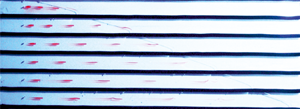
Figure 10. Evolution of slugs of unitary width released at $T=5$ in the interval $X\in [0-1]$ in a 10-layer aquifer, with $P+r-1=1$ for (a) a power-law fluid with $n=0.5$, (b) a power-law fluid with $n=0.7$ and (c) a Newtonian fluid. The grey lines are the trajectories of the front and of the back of the slug.

Figure 11 illustrates the slug evolution over time and space for fluids with a different behaviour index. The centre of mass of the slug advances and the dispersion generally increases in time. The direct comparison between fluids with a different $n$ is impractical in dimensionless coordinates since the velocity and time scales are different.

Figure 11. The advancement of a finite slug released at $T=5$ and of unitary width $X\in [0,1]$. (a) Snapshots at $T=5,100,500,1000$ for a power-law fluid with $n=0.5$; (b) and (c) as in (a) for a power-law fluid with $n=0.7$ and for a Newtonian fluid, respectively.

In order to evaluate longitudinal macro-dispersion, we consider the ratio between the standard deviation and the centre of mass of the slugs in different layers, assuming that the mass of each slug is concentrated in its own centre of mass, hence neglecting local dispersion occurring for the single slug (a comparison between the two phenomena is performed later). The centre of mass of the slugs is

(4.13)\begin{equation} \bar{X}\approx\dfrac{\displaystyle\sum_{r=1}^N{X_rA_r}}{\displaystyle\sum_{r=1}^N{A_r}}, \end{equation}

where $X_r$ and $A_r$ are the centre of mass and the mass of the slug in the $r$-th layer. The variance (second spatial moment of the solute cloud) is

(4.14)\begin{equation} \sigma^2\approx\dfrac{\displaystyle\sum_{r=1}^N{\left(X_r-\bar{X}\right)^2A_r}}{\displaystyle\sum_{r=1}^N{A_r}}, \end{equation}

and the ratio STD/mean is equal to $\sigma /\bar {X}$.

An approximate expression for the centre of mass and variance can be derived as follows. We assume that the slugs are released by injecting fluid in the same section for a finite-time interval. The mass of the slug in the $r$-th layer varies as the volume flux in that layer, which is proportional to $(P+r-1)^{1/n}/\eta _s^{1/n}$; see (2.8). Equation (2.19) can be approximated as

(4.15a,b)\begin{equation} \eta_f\approx \left(P+r+\dfrac{n}{2}\right)^{1/(n+1)}, \quad \eta_s\approx\eta_f-\dfrac{1}{\eta_f^n}; \end{equation}

hence, the mass of the slug scales with $\eta _f$. The position of the slug is also proportional to $\eta _f$, see (4.12) for the special case $n=1/2$; therefore, the centre of mass of the $N$ slugs varies as

(4.16)\begin{equation} \dfrac{\bar{X}}{\left(\dfrac{n+1}{n}T\right)^{n/(n+1)}}\approx\dfrac{\displaystyle\sum_{r=1}^N\eta_{f,r}^2}{\displaystyle\sum_{r=1}^N\eta_{f,r}}, \end{equation}

and the variance with respect to the centre of mass varies as

(4.17)\begin{equation} \dfrac{\sigma^2}{\left(\dfrac{n+1}{n}T\right)^{2n/(n+1)}}\approx\dfrac{\displaystyle\sum_{r=1}^N\eta_{f,r}^3}{\displaystyle\sum_{r=1}^N\eta_{f,r}} -\dfrac{\bar{X}^2}{\left(\dfrac{n+1}{n}T\right)^{2n/(n+1)}}. \end{equation}

Hence, the approximate relations based on summations are

(4.18)\begin{equation} \dfrac{\bar{X}}{\left(\dfrac{n+1}{n}T\right)^{n/(n+1)}}\approx\dfrac{(n+2)}{(n+3)}\dfrac{ \left(\dfrac{n}{2}+N+P\right)^{({n+3})/({n+1})}-\left(\dfrac{n}{2}+P\right)^{({n+3})/({n+1})}}{ \left(\dfrac{n}{2}+N+P\right)^{({n+2})/({n+1})}-\left(\dfrac{n}{2}+P\right)^{({n+2})/({n+1})}} \end{equation}

and

(4.19)\begin{align} \dfrac{\sigma^2}{\left(\dfrac{n+1}{n}T\right)^{2n/(n+1)}}&\approx \dfrac{(n+2)}{(n+4)}\frac{ \left(\dfrac{n}{2}+N+P\right)^{({n+4})/({n+1})}-\left(\dfrac{n}{2}+P\right)^{({n+4})/({n+1})}}{ \left(\dfrac{n}{2}+N+P\right)^{({n+2})/({n+1})}-\left(\dfrac{n}{2}+P\right)^{({n+2})/({n+1})} }\nonumber\\ &\quad -\left[\dfrac{(n+2)}{(n+3)}\dfrac{ \left(\dfrac{n}{2}+N+P\right)^{({n+3})/({n+1})}-\left(\dfrac{n}{2}+P\right)^{({n+3})/({n+1})}}{ \left(\dfrac{n}{2}+N+P\right)^{({n+2})/({n+1})}-\left(\dfrac{n}{2}+P\right)^{({n+2})/({n+1})}}\right]^2. \end{align}

The approximate time scalings from (4.18) to (4.19), $\bar {X} \sim T^{n/(n+1)}$ and $\sigma ^2 \sim T^{2n/(n+1)}$, reduce to $\bar {X} \sim \mathrm {const}$ and $\sigma ^2 \sim \mathrm {const}$ for $n \rightarrow 0$, and to $\bar {X} \sim T$, $\sigma ^2 \sim T^2$ for $n \rightarrow \infty$. For $n=1$, they collapse to the expressions given by Farcas & Woods (Reference Farcas and Woods2015) with $\bar {X} \sim T^{1/2}$, $\sigma ^2 \sim T$. The time scaling of the variance is sublinear for shear-thinning fluids with $n<1$, and supralinear for shear-thickening fluids with $n>1$. Correspondingly, one could define a longitudinal macro-dispersion coefficient $D_{LM}$ according to the classical definition $1/2 \times \text {d}(\sigma ^2)/\text {d}t$, and $D_{LM}$ would scale with time as $T^{(n-1)/(n+1)}$.

Figure 12(a) shows the exact values (derived via integration of the differential problem) of the ratio $\sigma /\bar {X}$, a measure of dispersion, for an aquifer with $N=10$ layers. For large overpressure $P$, the ratio is almost the same for all fluids, with slightly higher values for shear-thinning fluids, and asymptotically reaches a common value ${\approx }5\,\%$. Variation over time in the examined range is negligible, with results at $T=100$ almost coincident with the results at $T=1000$. In terms of dispersion, these results indicate that the length scale of the tracer cloud scales with time identically to the position of the centre of mass, being asymptotically a constant fraction (here approximately $5\,\%$) of the distance travelled by the plume. However, since the differences addressed to the $n$ fluid behaviour index are modest, the data field obtained with different fluids can be hardly useful to detect the aquifer structure. Figure 12(b) shows also the approximated values of $\sigma /\bar {X}$ (bold curves) according to (4.18) and (4.19). The approximation is fairly good providing that the overpressure $P$ is sufficiently high.

Figure 12. Comparison of the ratio of the standard deviation to the mean as a function of the overpressure $P$ for fluids with a different behaviour index $n$ at (a) $T=100$ and (b) at $T=1000$. The aquifer has $N=10$ layers and the slug of unitary width is released at $T=5$. Dashed curves refer to numerical computation, bold curves refer to the approximation in (4.18) and (4.19).

Figure 13(a) plots again the ratio $\sigma /\bar {X}$ for fluids with different fluid behaviour index $n$ as a function of overpressure $P$ and number of layers $N$, the total height being the same. Smaller values refer to a Newtonian fluid, whilst shear-thinning fluids favour larger dispersion values. Minimum dispersion is obtained with large $P$ and a limited number of layers ($\sigma /\bar {X}=0$ for a single layer), maximum dispersion corresponds to reduced overpressure $P$ values and many layers. Figure 13(b) compares $\sigma /\bar {X}$ for varying $N$ and $n$, with $P=N$. Shear-thinning fluids slightly increase dispersion with respect to a Newtonian fluid.

Figure 13. (a) Comparison of the asymptotic ratio $\sigma /\bar {X}$ for varying overpressure $P$ and number of layers $N$, and for fluids with $n=0.5,0.7,1$. Contours refer to $\sigma /\bar {X}=5\,\%$ (bold curves), $10\,\%$ (dashed curves), $15\,\%$ (dash–dotted curves), $20\,\%$ (dash–dot–dot curves) and $25\,\%$ (dotted curves). (b) The variation of the asymptotic ratio $\sigma /\bar {X}$ for varying $n$ and varying overpressure $P$, with a number of layers $N=P$.

These comparisons do not involve scales, and depend only on $n$, although the dimensional time required to reach the asymptotes depends on the time scale given by (2.2) or (A 10) that, in turn, are related to the nature of the medium (fractured or porous), its geometry and the rheological and physical properties of the fluid.

To compare large-scale (inter-layer) dispersion thus examined with local (intra-layer) transport phenomena, we recall that for power-law flow in porous media of grain size $\delta$ and flow speed $u$ the Peclet number is (Delgado Reference Delgado2006)

(4.20)\begin{equation} Pe = u \delta/D_L =0.2+0.011 Re^{0.48}_n = 0.2+0.011 \left(\dfrac{\rho \delta^n u^{2-n}}{\mu_0}\right)^{0.48}, \end{equation}

where $D_L$ is the (local) longitudinal dispersion coefficient. With $\delta = 10^{-4} \ \mathrm {m}$, $u \approx 10^{-7} \ \mathrm {m}\,\text {s}^{-1}$, $\rho \approx 1000 \ \mathrm {kg}\,\text {m}^{-3}$, $\mu _0 \approx 1 \ \mathrm {Pa} \, \text {s}^{{n}}$ and $n \approx 0.5$, the second term in (4.20) is negligible and hence $D_L \sim \delta u$. According to (4.6), for a power-law fluid in a porous layer, the velocity scales with time as

(4.21)\begin{equation} u \sim \dfrac{H^{1/(n+1)} V^{n/(n+1)}}{t^{1/(n+1)}}, \end{equation}

with $H$ and $V$ being length and velocity scales. Coupling these two results leads to the relationship

(4.22)\begin{equation} L \sim \delta^{1/2} H^{1/(2(n+1))} V^{n/(2(n+1))} t^{n/(2(n+1))} \end{equation}

for the typical length scale of a localised slug of tracer. On the other hand, (4.19) yields

(4.23)\begin{equation} L \sim H^{1/(n+1)} V^{n/(n+1)} t^{n/(n+1)} \end{equation}

for the length scale of the cloud of tracer slugs. Comparing the two scales, macro-dispersion prevails when

(4.24)\begin{equation} t \gg t_0 \equiv \dfrac{\delta^{(n+1)/n}}{H^{1/n}V}. \end{equation}

In a field setting, $H \approx 1 \ \mathrm {m}$, $V \approx 10^{-7} \ \mathrm {m}\,\text {s}^{-1}$, and with $\delta = 10^{-4} \ \mathrm {m}$ this yields $t_0 = 10^{-5} \ \mathrm {s}$ for $n = 0.5$, $t_0 = 0.1 \ \mathrm {s}$ for $n = 1$ and $t_0 = 2.15 \ \mathrm {s}$ for $n = 1.5$, showing the high sensitivity of threshold time $t_0$ to the value of $n$ in the shear-thinning range.

In a layered HS cell or fracture of gap $b$, the scalings are partially different as $D_L \sim (\bar {u}^2b^2)/D_0$ (Dejam Reference Dejam2019), where $D_0$ is the molecular diffusion coefficient; this leads to

(4.25)\begin{equation} L \sim \dfrac{1}{D_0} b H^{1/(n+1)} V^{n/(n+1)} t^{(n-1)/(2(n+1))} \end{equation}

for the length scale of a localised slug. The typical length scale of the solute cloud is unchanged, hence the condition for the macro-dispersion to prevail is independent from scales $H$, $V$ and flow behaviour index $n$ and reads $t \gg t_0 \equiv b^2/D_0$. With $b = 10^{-3} \ \mathrm {m}$ and $D_0 \approx 10^{-9}\ \mathrm {m}^2\,\text {s}^{-1}$, one has a threshold time of the order of $10^3 \ \mathrm {s}$.

5. The experiments

In order to validate the theoretical model, a set of experiments were conducted in a Hele-Shaw cell with a small gap, simulating a layered fracture. Figure 14 shows the experimental device, a $75\ \mathrm {cm}$ long, $18\ \mathrm {cm}$ high cell made of two parallel plates of transparent plastic, separated by a gap $b=0.25\ \text {cm}$. Six layers, each with height $1.9\ \mathrm {cm}$, were separated with sealing baffles. On one side, a large well, fed either by a vane pump or a small tank (for higher viscosity fluids) and having an overflow, guarantees a constant overpressure during fluid propagation. A lock gate (a plastic tube acting as an O-ring) was initially put in place and then fast removed at the start of the experiment. The profiles of the advancing noses of the current in the layers were detected with a high-resolution video camera (Canon Legria $1920 \times 1080$ pixels) operating at $25\ \mathrm {frames}\,\mathrm {s}^{-1}$ and with a single shot camera (Canon EOS 2D, $3456\times 2304$ pixels). The images, extracted with a varying time step according to the speed of the current, were then post-processed in order to be referenced to a lab coordinate system. With this set-up, the overall accuracy in detecting the profile of the current was approximately $0.1\ \text {cm}$, whilst the uncertainty in measuring timings was negligible.

Figure 14. A sketch of the Hele-Shaw cell. Front (a) and side (b) view, and (c) a snapshot.

A first set of experiments was conducted with Newtonian fluids, a second set with power-law shear-thinning fluids and a third set with Herschel–Bulkley fluids. Newtonian fluids were glycerol and a mixture of water and glycerol, power-law fluids were obtained by adding Xanthan Gum with different concentration, HB fluids were obtained by mixing deionized water, Carbopol 980 ($0.05\text {--}0.14\,\%$), ink, with subsequent neutralization by adding NaOH. The mass density was measured with a hydrometer (STV3500/23 Salmoiraghi) or with a pycnometer, or with a DMA 5000 by Anton Paar, with an accuracy $\Delta \rho /\rho \le 0.1\,\%$. The rheologic behaviour of the fluid was analysed with a Ubbelohde viscometer and with a parallel plate rheometer (Anton Paar Physica MCR 101) conducting several different tests to evaluate the fluid behaviour index (for power-law and HB fluids), the consistency index and the yield stress (for HB fluids). Figure 15(a,b) shows the shear-stress/shear-rate experimental data and the apparent viscosity, respectively, for five measurements taken for the same power-law fluid, three at $\varTheta =22\ ^{\circ }\text {C}$ and two at $\varTheta =24\ ^{\circ }\text {C}$. There is an adequate repeatability of the data and a minor dependence on temperature, with apparent viscosity decreasing with increasing temperature. It is also evident that the range of shear rate considered for interpolation affects the values of the consistency index $\mu _0$ and of the fluid behaviour index $n$, which is smaller in the low shear-rate domain. The estimated accuracy is $\Delta n/n\le 4.5\,\%$, $\Delta \mu _0/\mu _0\le 7\,\%$ and $\Delta \tau _p/\tau _p\le 10\,\%$. The parameters of the experiments are listed in table 1.

Figure 15. Rheometry measurements for the power-law fluid used in experiment 8. (a) Shear-stress/shear-rate experimental values and (b) apparent viscosity. Open circles refer to measurements at $\varTheta =24\ ^{\circ }\text {C}$, stars refer to measurements at $\varTheta =22\ ^{\circ }\text {C}$. The bold line is the interpolation for high shear rates, with $n=0.39$ and $\mu _0=0.87\ \text {Pa}\,\text {s}^n$, the dashed line is the interpolation for low shear rates, with $n=0.36$ and $\mu _0=0.91\ \text {Pa}\,\text {s}^n$.

Table 1. Parameters for the experiments in a layered cell/fracture. The last column indicates if tracer was injected at $x=7.2\ \text {cm}$.

Figure 16 shows three snapshots of experiment 7 with power-law fluids and $N=6$ layers. It is evident the different speed of the current in the layers and the different shape of the nose, more elongated for the upper than for the lower layers.

Figure 16. Three snapshots of experiment 7. Photographs were taken 1, 5, 10 s after the removal of the gate lock.

Figure 17(a,b) shows the nose front position $X_f$ and the limit of the pressurized current $X_s$ within the six layers for a Newtonian and a power-law fluid, respectively. The agreement between theory and experiments improves with time, as a consequence of the asymptotic intermediate self-similarity of the theoretical model. A similar behaviour is shown in figure 18(a,b), depicting the front position of the nose and the limits of the pressurized current in the six layers for a HB fluid. Again, experimental values tend asymptotically to theoretical ones, faster for the lower layers and with a slightly better match for the nose position than for the upper layers.

Figure 17. Dimensionless positions of the nose front and of the limit of pressurized current (a) for experiment 4 with a Newtonian fluid and (b) for experiment 7, a power-law fluid. The green lines refer to the theoretical nose front $X_f$, the red lines refer to the theoretical limit of the pressurized current $X_s$, the symbols are the experiments. Data for $X_f$ are translated in the vertical of 10 units for an easy visualization.

Figure 18. Dimensionless front positions for experiment 11 with an HB fluid. (a) Front position at contact with the bottom and (b) limit of the pressurized current. The lines are the theoretical values, the symbols are the experiments.

There is initially a certain discrepancy between theory and experiments; table 2 summarizes for three selected experiments with N, PL and HB fluids, the minimum (for upper layers) and maximum (for lower layers) relative error for the position of the pressurized body $X_s$ and of the nose $X_f$ at $t = 180\ \text {s}$ for Newtonian and power-law fluids, and at $t = 18\ \text {s}$ for the Herschel–Bulkley fluid (the HB experiments are shorter); corresponding root-mean square relative errors averaged over the remaining duration of each experiment are also listed. The error at $t = 180\ \text {s}$ is slightly larger for power-law fluids than for Newtonian, and lowest (at $t = 18\ \text {s}$) for HB fluids for both body and nose. The error in the late portion of the experiments follows the same trend but somewhat decreases.

Table 2. Minimum and maximum relative error in the six layers for the position of the pressurized body $X_s$ and of the nose $X_f$, computed as $\Delta _{X_s}= \vert X_{s-exp}-X_{s-th} \vert / X_{s-th}$ and $\Delta _{ X_f} = \vert X_{f-exp}-X_{f-th} \vert / X_{f-th}$ at $t=180\ \text {s}$ for N and PL, at $t=18\ \text {s}$ for HB, respectively. The third and fourth columns $\overline {\Delta _{X_s}}$ and $\overline {\Delta _{X_f}}$ list the root mean square values for $t>180\ \text {s}$ (till the end of each experiment) for N and PL fluid experiments, and for $t>18\ \text {s}$ for the HB fluid experiment. Here N, PL and HB stands for Newtonian, power-law and Herschel–Bulkley fluid, respectively.

By observing figures 17(a,b) and 18(a,b) one would conclude that experiments with Newtonian and PL fluids show a better agreement with theory than those with HB fluids, with a faster approach to intermediate asymptotics. Data listed in table 2 indicate that the opposite is true, with the HB fluid experiment showing less deviation from the theory than the Newtonian and PL fluid experiments. However, this last result is odd and cannot be generalized since HB fluid experiments are expected to deviate from theory more than the Newtonian and PL fluid experiments, as a consequence of (i) model approximations, as the solution for HB fluids is based on an expansion of the self-similar solution for PL fluids; (ii) the accuracy of rheometric measurements, which are known to be less accurate in the presence of yield stress; (iii) possible slip at the wall. Further sources of discrepancy common to experiments with PL and HB fluids are effects missing in the model, such as surface tension phenomena in the nose and inaccuracies in the channel geometry. Finally, there is an intrinsic approximation in the adoption of relatively simple constitutive equations (2/3 parameters for PL/HB fluids) to interpret non-Newtonian behaviour over a wide range of shear rates. More complex rheological models could give a better fit to the experiments. We also recall the difficulty in comparing experiments where the rheology and duration is different.

Figure 19 shows the flow front for experiment 9, PL fluid, and for experiment 12, HB fluid, rescaled to the value $\eta =X/[T(n+1)/n]^{n/(n+1)}$ and $\eta =X/[T(n+1)/n]^{n/(n+1)}(1+\psi \chi _1)$, respectively, and the vertical position from the base of the cell has been rescaled to the interval $[0,1]$. The collapse to a single curve, predicted by the theory, is better for PL than for HB fluids, improves in time and with the overpressure (the depth) of the layer.

Figure 19. Comparison of the experimental data for the height of the current as a function of the distance from the source with the theoretical prediction. (a) Experiment 9, power-law fluid and (b) experiment 12, Herschel–Bulkley fluid. The horizontal axis shows the dimensionless $\eta$ from (2.12a,b) and from (3.11), respectively. The experimental data refer to different times as shown in the legend, the curves refer to the theoretical model.

In a subset of experiments, conducted with Newtonian and power-law fluids, pulses of tracer were simultaneously injected in the six layers at mid-height and mid-width and a distance $x=7.2\ \text {cm}$ from the origin, in order to validate the model for the transport properties of the domain.

Figure 20 shows the migration of four series of pulses injected in the flow during an experiment with a power-law fluid. The pulses travel noticeably faster than the mean velocity of the current, elongate during travel, spread little in the other two directions and tend to accumulate near the front when they reach the nose. There is specific evidence that the injected tracer concentrates at the mid gap position; see figure 21 where the red shadow of the slugs is visible on the back wall of the Hele-Shaw cell. The slug advances like a comet, with the tail due to the transversely diffused fluid that moves towards areas near the walls characterized by a lower speed. In correspondence of the axis of the cell the shear rate tends to zero reducing the dispersion of the slug nose, which maintains its structure and advances with a reduced loss of mass. In the nose the tracer is convected down to the bottom of the layer, see the coloured nose of the upper layer, and the flow field is three-dimensional, hence cannot be properly described within the present model.

Figure 20. A snapshot of experiment 9, power-law fluid, at $t=35\ \text {s}$. The circles are the injection points, the dashed curves are the envelopes of the slugs generated by four injections at $t=7, 15, 25, 33\ \text {s}$, synoptic for all layers.

Figure 21. A snapshot of experiment 10, power-law fluid. The shadow projected by the slugs on the back wall indicates that the slugs do not fill the entire gap of the cell. Photographs was taken 15 s after the removal of the gate lock.

Faster plumes in lower layers spread more in the longitudinal direction due to increased shear dispersion, proportional to mean velocity squared for pressurized flow of Newtonian (Berkowitz & Zhou Reference Berkowitz and Zhou1996) and power-law fluids (Dejam Reference Dejam2019) in a single fracture. An order of magnitude analysis based on the latter formulation confirms shear dispersion prevails over molecular diffusion; the Peclet number $Pe = \bar {u}(b/2)/D_0$ in each fracture is of order $5 \times 10^3 \ \text {s}$ (with mean velocity $\bar {u}=0.005 \ \text {m}\,\text {s}^{-1}$, half-gap $b/2 = 1.25 \times 10^{-3} \ \text {m}$ and diffusion coefficient in water $D_0 \approx 10^{-9} \ \text {m}^2\,\text {s}^{-1}$); the diffusion time across the gap is $t_D=(b/2)^2/D_0$, decidedly larger than the duration of the experiments. As all evidence confirms that each pulse remains localized at the centre of the current, the comparison with the experiments is drawn considering the actual path of particles by introducing the maximum speed of the current in (4.6), with $U_{max}/U=(2n+1)/(n+1)$.

Figure 22 shows a comparison of $X_s$, $X_f$ and of the path of the slugs for $r=1,3,6$. The experimental position of the slugs is still ahead of the theoretical one, as a consequence of secondary effects such as the lack of symmetry of the velocity field with respect to the fully confined scheme, leading to enhanced dispersion, but the agreement is quite satisfactory for slugs advancing in the pressurised portion of the current (all series of injections in layers $r=3$ and $r=6$ and for $i2$, $i3$ and $i4$ for layer $r=1$) and in the nose (injection $i1$ for layer $r=1$).

Figure 22. Advancement of the slugs for experiment 5, Newtonian fluid. (a) Experimental $X_s$ (orange x) and $X_f$ (green +), and slug position at four different time of injection ($i1,i2,i3,i4$) for $r=1$, (b) for $r=3$, and (c) for $r=6$. Symbols are experimental data, curves are theoretical values.