


No CrossRef data available.
Article contents
Drift, diffusion and divergence
Published online by Cambridge University Press: 27 May 2025
Abstract
Turbulent Taylor–Couette flow displays traces of axisymmetric Taylor vortices even at high Reynolds numbers. With this motivation, Feldmann & Avila (2025) J. Fluid Mech, 1008, R1, carry out long-time numerical simulations of axisymmetric high-Reynolds-number Taylor–Couette flow. They find that the Taylor vortices, using the only degree of freedom that remains available to them, carry out Brownian motion in the axial direction, with a diffusion constant that diverges as the number of rolls is reduced below a critical value.
JFM classification
Information
- Type
- Focus on Fluids
- Information
- Creative Commons


 This is an Open Access article, distributed under the terms of the Creative Commons Attribution-ShareAlike licence (https://creativecommons.org/licenses/by-sa/4.0/), which permits re-use, distribution, and reproduction in any medium, provided the same Creative Commons licence is used to distribute the re-used or adapted article and the original article is properly cited.
- Copyright
- © The Author(s), 2025. Published by Cambridge University Press
References
Akinaga, T., Generalis, S.C. & Busse, F.H. 2018 Tertiary and quaternary states in the Taylor–Couette system. Chaos, Solitons Fractals 109, 107–117.10.1016/j.chaos.2018.01.033CrossRefGoogle Scholar
Altmeyer, S., Do, Y., Marques, F. & Lopez, J.M. 2012 Symmetry-breaking Hopf bifurcations to 1-, 2-, and 3-tori in small-aspect-ratio counterrotating Taylor-Couette flow. Phys. Rev. E
86, 046316.10.1103/PhysRevE.86.046316CrossRefGoogle ScholarPubMed
Andereck, C.D., Liu, S.S. & Swinney, H.L. 1986 Flow regimes in a circular Couette system with independently rotating cylinders. J. Fluid Mech. 164, 155–183.10.1017/S0022112086002513CrossRefGoogle Scholar
Chossat, P. & Iooss, G. 1994 The Couette–Taylor Problem. Springer-Verlag.10.1007/978-1-4612-4300-7CrossRefGoogle Scholar
Coles, D. 1965 Transition in circular Couette flow. J. Fluid Mech. 21, 385–425.10.1017/S0022112065000241CrossRefGoogle Scholar
Deguchi, K. & Altmeyer, S. 2013 Fully nonlinear mode competitions of nearly bicritical spiral or Taylor vortices in Taylor–Couette flow. Phys. Rev. E
87, 043017.10.1103/PhysRevE.87.043017CrossRefGoogle ScholarPubMed
Dong, S. 2007 Direct numerical simulation of turbulent Taylor–Couette flow. J. Fluid Mech. 587, 373–393.10.1017/S0022112007007367CrossRefGoogle Scholar
Dubrulle, B., Dauchot, O., Daviaud, F., Longaretti, P.-Y., Richard, D. & Zahn, J.-P. 2005 Stability and turbulent transport in Taylor–Couette flow from analysis of experimental data. Phys. Fluids 17, 095103.10.1063/1.2008999CrossRefGoogle Scholar
Eckhardt, B., Doering, C.R. & Whitehead, J.P. 2020 Exact relations between Rayleigh–Bénard and rotating plane Couette flow in two dimensions. J. Fluid Mech. 903, R4.10.1017/jfm.2020.718CrossRefGoogle Scholar
Edwards, W., Tagg, R., Dornblaser, B., Swinney, H.L. & Tuckerman, L. 1991 Periodic traveling waves with nonperiodic pressure. Eur. J. Mech. B/Fluids 10, 205–210.Google Scholar
Feldmann, D. & Avila, M. 2025 Taylor rolls on tour: slow drift of turbulent large-scale structures in flows with continuous symmetries. J. Fluid Mech. 1008, R1.10.1017/jfm.2025.135CrossRefGoogle Scholar
Goharzadeh, A. & Mutabazi, I. 2001 Experimental characterization of intermittency regimes in the Couette–Taylor system. Eur. Phys. J. B
19, 157–162.10.1007/s100510170360CrossRefGoogle Scholar
Grossmann, S., Lohse, D. & Sun, C. 2016 High-Reynolds number Taylor–Couette turbulence. Annu. Rev. Fluid Mech. 48, 53–80.10.1146/annurev-fluid-122414-034353CrossRefGoogle Scholar
Huisman, S.G., Van Der Veen, R.C., Sun, C. & Lohse, D. 2014 Multiple states in highly turbulent Taylor–Couette flow. Nat. Commun. 5, 3820.10.1038/ncomms4820CrossRefGoogle ScholarPubMed
Kreilos, T., Zammert, S. & Eckhardt, B. 2014 Comoving frames and symmetry-related motions in parallel shear flows. J. Fluid Mech. 751, 685–697.10.1017/jfm.2014.305CrossRefGoogle Scholar
Lathrop, D.P., Fineberg, J. & Swinney, H.L. 1992 Transition to shear-driven turbulence in Couette–Taylor flow. Phys. Rev. A
46, 6390–6405.10.1103/PhysRevA.46.6390CrossRefGoogle ScholarPubMed
Lemoult, G., Shi, L., Avila, K., Jalikop, S.V., Avila, M. & Hof, B. 2016 Directed percolation phase transition to sustained turbulence in Couette flow. Nat. Phys. 12, 254–258.10.1038/nphys3675CrossRefGoogle Scholar
Prigent, A., Gregoire, G., Chaté, H., Dauchot, O. & van Saarloos, W. 2002 Large-scale finite-wavelength modulation within turbulent shear flows. Phys. Rev. Lett. 89, 014501.10.1103/PhysRevLett.89.014501CrossRefGoogle ScholarPubMed
Shi, L., Avila, M. & Hof, B. 2013 Scale invariance at the onset of turbulence in Couette flow. Phys. Rev. Lett. 110, 204502.10.1103/PhysRevLett.110.204502CrossRefGoogle ScholarPubMed
Taylor, G. 1923 Stability of a viscous fluid contained between two rotating cylinders. Phil. Trans. R. Soc. Lond. A
223, 289–343.Google Scholar
Veronis, G. 1970 The analogy between rotating and stratified fluids. Annu. Rev. Fluid Mech. 2, 37–66.10.1146/annurev.fl.02.010170.000345CrossRefGoogle Scholar
Weisshaar, E., Busse, F. & Nagata, M. 1991 Twist vortices and their instabilities in the Taylor–Couette system. J. Fluid Mech. 226, 549–564.10.1017/S0022112091002501CrossRefGoogle Scholar
Xi, H.-D., Zhou, Q. & Xia, K.-Q. 2006 Azimuthal motion of the mean wind in turbulent thermal convection. Phys. Rev. E
73, 056312.10.1103/PhysRevE.73.056312CrossRefGoogle ScholarPubMed

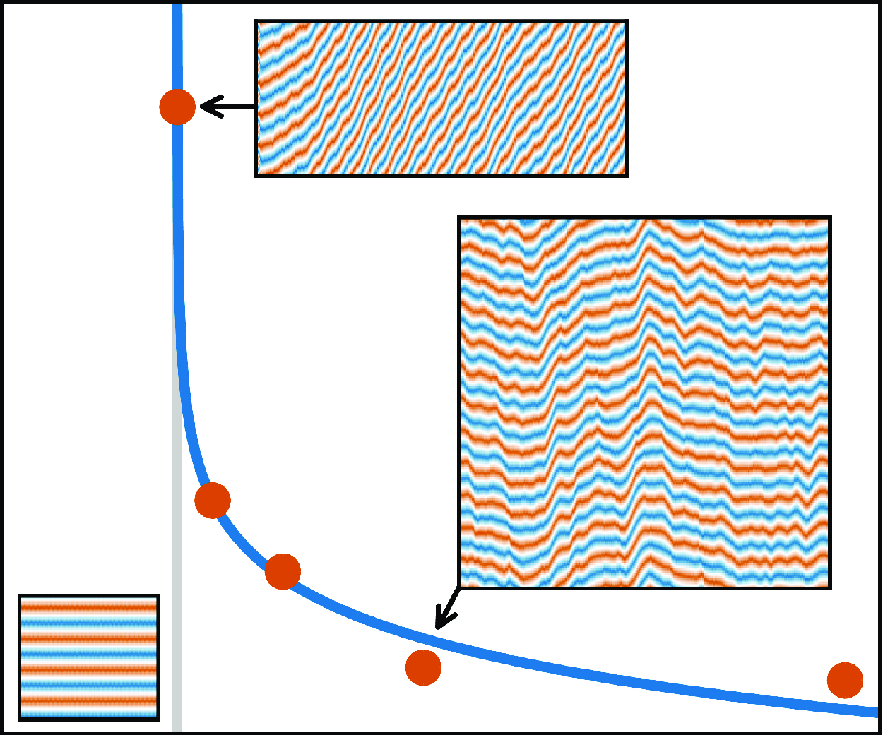
Figure 1. Temporal evolution of radial velocity along an axial line at mid-gap. The aspect ratio  $\Gamma$ of axial length to radial gap corresponds to the number of vortices. For $\Gamma =8$, after an initial transient, the vortices do not move, while for $\Gamma =10$, they move very quickly in one direction. For $\Gamma =12$ and 24, the vortices sporadically change their direction of motion. From Feldmann & Avila (2025).
 You have
Access
You have
Access
 Open access
1. Introduction
In 1923, Taylor published his ground-breaking experiment and linear stability calculation, whose agreement demonstrated the validity of the Navier–Stokes equations. Since then, Taylor–Couette flow has served as one of the protypical systems in fluid dynamics. In the Taylor–Couette experiment, fluid is confined between two concentric cylinders which rotate at different angular velocities. In laminar Taylor–Couette flow, the motion is purely azimuthal and fluid particles at different radii do not mix. Increasing the angular velocity difference past a critical value leads to the formation of Taylor vortices, toroidal rolls in which circular motion in the meridional $(r,z)$
plane redistributes fluid and angular momentum between the radii.
$(r,z)$
plane redistributes fluid and angular momentum between the radii.
Ever since Taylor described and explained the onset of axisymmetric Taylor-vortex flow, an extravagant profusion of three-dimensional patterns of extraordinary variety, beauty and complexity have been discovered experimentally and numerically (e.g. Andereck et al. Reference Andereck, Liu and Swinney1986; Weisshaar et al. Reference Weisshaar, Busse and Nagata1991; Chossat & Iooss Reference Chossat and Iooss1994; Altmeyer et al. Reference Altmeyer, Do, Marques and Lopez2012; Deguchi & Altmeyer Reference Deguchi and Altmeyer2013; Akinaga et al. Reference Akinaga, Generalis and Busse2018). The mathematics of what is called variously equivariant bifurcation theory, symmetry and pattern formation has been brought to bear to predict and explain these spirals and ribbons, twists and waves, modulation and bursts.
Turbulence in Taylor–Couette flow has also been studied, both at high Reynolds number and in the transitional range at low Reynolds number (e.g. Coles Reference Coles1965; Goharzadeh & Mutabazi Reference Goharzadeh and Mutabazi2001; Prigent et al. Reference Prigent, Gregoire, Chaté, Dauchot and van Saarloos2002; Shi et al. Reference Shi, Avila and Hof2013; Lemoult et al. Reference Lemoult, Shi, Avila, Jalikop, Avila and Hof2016). But who would have thought that there was something new to be learned about turbulence from axisymmetric Taylor–Couette flow?
2. Summary of paper
It has long been known that the Taylor-vortex structure persists even far into the turbulent regime, i.e. that turbulence is superposed on Taylor vortices (e.g. Lathrop et al. Reference Lathrop, Fineberg and Swinney1992; Dong Reference Dong2007; Huisman et al. Reference Huisman, Van Der Veen, Sun and Lohse2014; Grossmann et al. Reference Grossmann, Lohse and Sun2016); long-time averaging accentuates the features of these ghostly vortices. Eckhardt et al. (Reference Eckhardt, Doering and Whitehead2020) have argued that, under certain hypotheses, transport of angular momentum by chaotic fluctuations in axisymmetric Taylor–Couette flow reproduces the transport associated with the axisymmetric component of turbulent solutions to the full three-dimensional equations. This suggests that the axisymmetric problem could be viewed, not merely as a first step towards turbulence (laminar $\rightarrow$
axisymmetric Taylor-vortex flow
$\rightarrow$
axisymmetric Taylor-vortex flow $\rightarrow$
three-dimensional patterns
$\rightarrow$
three-dimensional patterns $\rightarrow$
turbulence), but as a model for its mean (necessarily axisymmetric) properties. Feldmann & Avila (Reference Feldmann and Avila2025) have carried out long-time axisymmetric simulations of Taylor–Couette flow as a possible route towards studying turbulent structures.
$\rightarrow$
turbulence), but as a model for its mean (necessarily axisymmetric) properties. Feldmann & Avila (Reference Feldmann and Avila2025) have carried out long-time axisymmetric simulations of Taylor–Couette flow as a possible route towards studying turbulent structures.
Axisymmetric Taylor-vortex flow consists of an axial stack of toroidal vortices. The vortices are approximately circular, so that the number of vortices is close to the axial-length-to-radial-gap ratio $\Gamma$
. Feldmann & Avila (Reference Feldmann and Avila2025) observe that the number of vortices remains constant over the course of a simulation. Such a one-dimensional periodic structure is highly constrained and so its possible dynamics are limited: the only remaining possible motion is an axial jiggle or drift of the entire stack of vortices. Feldmann & Avila (Reference Feldmann and Avila2025) find that, for a relatively long system, the rolls carry out diffusive drift (Brownian motion) so that the variance of the phase grows linearly in time. Moreover, the effective diffusion coefficient diverges following a power law as a threshold axial length (or number of rolls)
$\Gamma$
. Feldmann & Avila (Reference Feldmann and Avila2025) observe that the number of vortices remains constant over the course of a simulation. Such a one-dimensional periodic structure is highly constrained and so its possible dynamics are limited: the only remaining possible motion is an axial jiggle or drift of the entire stack of vortices. Feldmann & Avila (Reference Feldmann and Avila2025) find that, for a relatively long system, the rolls carry out diffusive drift (Brownian motion) so that the variance of the phase grows linearly in time. Moreover, the effective diffusion coefficient diverges following a power law as a threshold axial length (or number of rolls) $\Gamma _c$
is approached from above. For a shorter axial length, although there may be an immediate adjustment of the position, the rolls quickly becomes quasi-stationary, with only weak chaotic motion about a fixed location. For the parameters used by Feldmann & Avila (Reference Feldmann and Avila2025),
$\Gamma _c$
is approached from above. For a shorter axial length, although there may be an immediate adjustment of the position, the rolls quickly becomes quasi-stationary, with only weak chaotic motion about a fixed location. For the parameters used by Feldmann & Avila (Reference Feldmann and Avila2025), $\Gamma _c=10$
; see figure 1. The significance of this sharp threshold is unknown.
$\Gamma _c=10$
; see figure 1. The significance of this sharp threshold is unknown.
Figure 1. Temporal evolution of radial velocity along an axial line at mid-gap. The aspect ratio $\Gamma$
of axial length to radial gap corresponds to the number of vortices. For
$\Gamma$
of axial length to radial gap corresponds to the number of vortices. For $\Gamma =8$
, after an initial transient, the vortices do not move, while for
$\Gamma =8$
, after an initial transient, the vortices do not move, while for $\Gamma =10$
, they move very quickly in one direction. For
$\Gamma =10$
, they move very quickly in one direction. For $\Gamma =12$
and 24, the vortices sporadically change their direction of motion. From Feldmann & Avila (Reference Feldmann and Avila2025).
$\Gamma =12$
and 24, the vortices sporadically change their direction of motion. From Feldmann & Avila (Reference Feldmann and Avila2025).
Although this is an interesting puzzle by itself, its importance is increased by its generality. Many hydrodynamic systems are driven by an imposed gradient of some quantity. Rolls appear as a means of redistributing this quantity: azimuthal or streamwise velocity for Taylor–Couette, plane Couette or Poiseuille flow, temperature for Rayleigh–Bénard convection, concentration for a binary fluid. Drift has been observed in these other systems (Xi et al. Reference Xi, Zhou and Xia2006; Kreilos et al. Reference Kreilos, Zammert and Eckhardt2014) and according to Feldmann & Avila (Reference Feldmann and Avila2025), the drift appears to be of the same type.
Exploiting the analogy between axisymmetric Taylor–Couette flow and two-dimensional Rayleigh–Bénard convection (Veronis Reference Veronis1970), Eckhardt et al. (Reference Eckhardt, Doering and Whitehead2020) have proposed a mapping from the two Reynolds numbers (inner and outer, or equivalently, shear $Re_S$
and rotation
$Re_S$
and rotation $R_\Omega$
(
$R_\Omega$
( $Re_S\equiv Ud/\nu$
and
$Re_S\equiv Ud/\nu$
and $R_\Omega\equiv 2d\Omega/U$
where
$R_\Omega\equiv 2d\Omega/U$
where $d$
is the gap width between the outer and inner cylinders,
$d$
is the gap width between the outer and inner cylinders, $\Omega$
is the angular velocity of the outer cylinder, and
$\Omega$
is the angular velocity of the outer cylinder, and $U$
is the difference between the angular velocities of the inner and outer cylinders times the inner cylinder radius.)) of Taylor–Couette flow (Dubrulle et al. Reference Dubrulle, Dauchot, Daviaud, Longaretti, Richard and Zahn2005) to the single Rayleigh number
$U$
is the difference between the angular velocities of the inner and outer cylinders times the inner cylinder radius.)) of Taylor–Couette flow (Dubrulle et al. Reference Dubrulle, Dauchot, Daviaud, Longaretti, Richard and Zahn2005) to the single Rayleigh number $Ra$
of Rayleigh–Bénard convection. Feldmann & Avila (Reference Feldmann and Avila2025) have provided support for this analogy by showing that the diffusion coefficient of the axial drift was the same for different parameter pairs
$Ra$
of Rayleigh–Bénard convection. Feldmann & Avila (Reference Feldmann and Avila2025) have provided support for this analogy by showing that the diffusion coefficient of the axial drift was the same for different parameter pairs $(Re_S,R_\Omega )$
yielding the same value of
$(Re_S,R_\Omega )$
yielding the same value of $Ra$
.
$Ra$
.
This demonstrates the interest in axisymmetric Taylor–Couette flow from a scientific point of view. However, the imposition of axisymmetry also has the great advantage of economy. Measuring diffusion coefficients of the axial drift requires extremely long times, especially if other parameters are varied as well, i.e. the number of rolls and the Reynolds numbers. Feldmann & Avila (Reference Feldmann and Avila2025) have been able to measure these diffusion coefficients because axisymmetric simulations require only a small fraction of the time that would be required to simulate the three-dimensional flow.
One might associate axial drift (motion of the phase) with axial flux (motion of fluid particles). To investigate this, Feldmann & Avila (Reference Feldmann and Avila2025) have compared simulations in which the axial flux is set to zero with those in which the net axial pressure gradient is zero. Either condition is valid for a periodic direction, but the choice has significant consequences if the flow is not reflection symmetric (e.g. Edwards et al. Reference Edwards, Tagg, Dornblaser, Swinney and Tuckerman1991). Feldmann & Avila (Reference Feldmann and Avila2025) find that in the absence of axial flux, the drift is considerably reduced, but still undergoes Brownian motion.
3. The future
Several questions are raised by this paper. The most obvious and perplexing is the reason for the abrupt threshold. Why are shorter columns tranquil and why are slightly longer columns suddenly so jittery? What physical phenomenon could be responsible for such a sharp distinction?
The second question concerns its generality. Feldmann & Avila (Reference Feldmann and Avila2025) have given convincing evidence that the rolls in other flows, such as Poiseuille flow, Rayleigh–Bénard convection and Taylor–Couette flow with no axial flux, also undergo diffusive drift. Does drift in these flows also have a length threshold? Are the threshold and the power law decay exponent the same?
The third question concerns the applicability of these axisymmetric results to the three-dimensional turbulence which naturally occurs at these high values of Reynolds or Rayleigh number. Eckhardt et al. (Reference Eckhardt, Doering and Whitehead2020) suggest that some global properties of three-dimensional turbulent Taylor–Couette flow could be captured by its axisymmetric analogue. Is axial drift one of those properties? What other properties might obey this?
Declaration of interests
The authors report no conflict of interest.