


1. Introduction
The application of a high-speed gas jet onto a liquid film or a droplet-laden surface is relevant in many industrial applications, such as coating and drying processes (Tuck Reference Tuck1983; Lacanette et al. Reference Lacanette, Gosset, Vincent, Buchlin and Arquis2006), oxygen steelmaking (Koria & Lange Reference Koria and Lange1984; Dogan, Brooks & Rhamdhani Reference Dogan, Brooks and Rhamdhani2009) and immersion lithography (Berendsen et al. Reference Berendsen, Zeegers, Kruis, Riepen and Darhuber2012). In particular, the complex behaviours of liquid films under gas flows have been studied in diverse contexts. Banks & Chandrasekhara (Reference Banks and Chandrasekhara1963) experimentally and theoretically determined the shape and size of the cavity formed in a liquid layer for varying jet speeds, as the air jet is applied from a nozzle. They also identified the formation of liquid drops as the jet velocity at the interface exceeds a critical value. A theoretical study by Rosler & Stewart (Reference Rosler and Stewart1968) identified three liquid film behaviours under a jet flow: stable, oscillating and dispersing cavities, as a function of the jet velocity and surface tension coefficient. In addition, there have been a series of theoretical studies (Moriarty, Schwartz & Tuck Reference Moriarty, Schwartz and Tuck1991; Mckinley, Wilson & Duffy Reference Mckinley, Wilson and Duffy1999; Mckinley & Wilson Reference Mckinley and Wilson2001) that consider the spreading of a liquid film under spin coating or, equivalently, under a vertical air jet. Berendsen et al. (Reference Berendsen, Zeegers, Kruis, Riepen and Darhuber2012) combined experiments and theory to study the dewetting phenomena and film rupture for thin liquid layers. Their results showed that the time of film ruptures depends on the Reynolds number, Re. More recently, Ojiako et al. (Reference Ojiako, Cimpeanu, Bandulasena, Smith and Tseluiko2020) studied the deformation and dewetting of liquid films under a gas jet with direct numerical simulation (DNS) and successfully compared the numerical results with experimental data.
In contrast to a high-speed gas jet impinging on a liquid layer, only a few studies have considered the effects of a high-Reynolds-number airflow on partially wetting droplets (Hooshanginejad & Lee Reference Hooshanginejad and Lee2017; Hooshanginejad et al. Reference Hooshanginejad, Dutcher, Shelley and Lee2020; White & Schmucker Reference White and Schmucker2021; Hooshanginejad & Lee Reference Hooshanginejad and Lee2022), most of which focus on uniform airflow parallel to the solid substrate. In this context, high-Reynolds-number airflows have Re of  $O(10^{2})$ or higher, where Re is associated with the external flow and the typical droplet size (Acarlar & Smith Reference Acarlar and Smith1987). Fan, Wilson & Kapur (Reference Fan, Wilson and Kapur2011) experimentally demonstrated that the critical jet speed leading to droplet motion is related to the contact angle and the droplet size. They also provided a theoretical model based on a force balance between the capillary forces at the contact line and the viscous stress induced by the airflow. Based on a diffuse-interface method, Ding, Gilani & Spelt (Reference Ding, Gilani and Spelt2010) numerically simulated the motion and deformation of a three-dimensional droplet on a solid substrate under an imposed shear flow and studied the critical condition for droplet entrainment. Seiler et al. (Reference Seiler, Gloerfeld, Roisman and Tropea2019) theoretically and experimentally studied droplet motion and the underlying force balance of a partially wetting droplet driven by a fully turbulent horizontal channel flow.
Distinct from the existing studies, Hooshanginejad & Lee (Reference Hooshanginejad and Lee2017) experimentally considered the effects of a more complex airflow on a partially wetting droplet by placing the droplet behind a solid hemispherical obstruction which separates the incoming airflow. Their results demonstrated that the droplet exhibits drafting, upstream motion and splitting, depending on the droplet's position relative to the reattachment length of the separated airflow. However, the pressure distribution inside the airflow is not described explicitly in their study.
More recently, Hooshanginejad et al. (Reference Hooshanginejad, Dutcher, Shelley and Lee2020) experimentally and theoretically investigated the dynamics of a partially wetting droplet when a jet of air is applied perpendicularly to the substrate. Their experiments revealed three distinct behaviours of the droplet: droplet oscillating in place, splitting and depinning to one side of the jet, depending on the strength and position of the jet. The authors also considered a lubrication model of the droplet with a fixed contact line under a two-dimensional stagnation-point flow. Although their model qualitatively captures the threshold of droplet splitting, there are two major shortcomings of their theoretical model. First, the model cannot reproduce the depinning behaviour of the droplet, as the contact line is fixed in place. Second, the stagnation-point flow used in the model does not correctly describe the decay of the jet speed away from the nozzle.
Inspired by the experiments and theory by Hooshanginejad et al. (Reference Hooshanginejad, Dutcher, Shelley and Lee2020), we develop a new lubrication model of the motion of a partially wetting droplet in the present study. The new model incorporates a moving contact line model with a precursor film and the disjoining pressure which accounts for the intermolecular interactions near the contact line (Schwartz Reference Schwartz1998; Espín & Kumar Reference Espín and Kumar2015; Park & Kumar Reference Park and Kumar2017). The presence of the precursor film eliminates a stress singularity that arises when the no-slip boundary is applied at the contact line (Huh & Scriven Reference Huh and Scriven1971; Savva & Kalliadasis Reference Savva and Kalliadasis2011). In addition, the disjoining pressure has been extensively used to model the liquid–solid interactions in thin films (Herminghaus et al. Reference Herminghaus, Jacobs, Mecke, Bischof, Fery, Ibn-Elhaj and Schlagowski1998), which is also relevant in the droplet breakup mechanism in our analysis. Another new feature of our model is the inclusion of a turbulent gas jet that is modelled as a self-similar Gaussian form with a decaying centreline speed (Kriegsmann, Miksis & Vanden-Broeck Reference Kriegsmann, Miksis and Vanden-Broeck1998; Schlichting & Gersten Reference Schlichting and Gersten2016). As the dominant effects of the turbulent jet on the droplet are through the imposed normal stress, we neglect the tangential stress in our model formulation (e.g. Lunz & Howell Reference Lunz and Howell2018). However, in a different regime, the effects of shear stress from the turbulent jet can be modelled based on an experimentally validated theoretical framework (Phares, Smedley & Flagan Reference Phares, Smedley and Flagan2000) or an empirical expression derived from the numerical simulations (Ojiako et al. Reference Ojiako, Cimpeanu, Bandulasena, Smith and Tseluiko2020).
Overall, our new model can reproduce macroscopic droplet behaviours, such as droplet splitting and depinning, as observed by Hooshanginejad et al. (Reference Hooshanginejad, Dutcher, Shelley and Lee2020), whereas it neglects fast-time-scale droplet oscillations. Our analysis also includes the steady-state solutions that rationalise the threshold of the droplet splitting and that of the droplet depinning. The paper is organised as follows: we introduce the formulation of the mathematical model and the numerical method in § 2. Section 3 comprises the results of the numerical simulations and the analytical solutions, in comparison with the experimental observations by Hooshanginejad et al. (Reference Hooshanginejad, Dutcher, Shelley and Lee2020). We conclude the paper with the summary and discussion in § 4.
2. Theory
2.1. Model set-up and assumptions
We construct a mathematical model based on the experiments by Hooshanginejad et al. (Reference Hooshanginejad, Dutcher, Shelley and Lee2020) and their characteristic parameters. The schematic of the model is shown in figure 1. In a two-dimensional system, we consider a water droplet (viscosity  $\mu _d = 8.9\times 10^{-4}\ {\rm Pa}\ {\rm s}$ and density $\rho _d = 997\,{\rm kg}\ {\rm m}^{-3}$) attached to a solid surface, where the shape of the droplet is specified as $h(x,t)$. The initial droplet half-width is given by $l$, whose typical value ranges from $1$ to $20\ {\rm mm}$, whereas the equilibrium contact angle $\theta _0$ is approximately $30^{\circ }$. A nozzle with a width $d_0$ is placed above the substrate with a vertical distance $H$, where $d_0 = 0.2\ {\rm mm}$ and $H=30\ {\rm mm}$ unless stated otherwise. The air jet from the nozzle has the magnitude $U_0$ that is varied from $5$ to $70\ {\rm m}\ {\rm s}^{-1}$, whereas the viscosity and density of air correspond to $\mu _a = 1.8\times 10^{-5}\ {\rm Pa}\ {\rm s}$ and $\rho _a = 1.2\ {\rm kg}\ {\rm m}^{-3}$, respectively. The horizontal distance between the centre of the nozzle and that of the droplet is characterised by a dimensionless parameter, $\alpha$, which has been normalised by $l$. Hence, $\alpha = 0$ corresponds to the case where the jet and the droplet are centred. As the nozzle is turned on, the air flow strikes the droplet surface, and the droplet starts to deform and spread, causing the contact line to move. The contact-line locations are specified as $x=s_1(t)$ and $x=-s_2(t)$. If the centre of the jet and the centre of the droplet are not aligned (i.e. $\alpha \ne 0$), then $s_1\neq s_2$. For $\alpha = 0$, we assume $s_1= s_2$ for simplicity, by neglecting the air jet fluctuations that may cause symmetry breaking.

Figure 1. Schematic of a two-dimensional partially wetting droplet that is deforming under an impinging jet with magnitude  $U_0$. The $x$-axis is parallel to the solid substrate, while the $z$-axis is normal to the substrate. The nozzle is located at a vertical distance $H$ from the substrate and has an opening width of $d_0$. The horizontal distance between the initial centre of the droplet and that of the nozzle corresponds to $\alpha l$. The shape of the deforming droplet is given by $h(x,t)$ with a precursor film with thickness $b$, subject to the external air pressure denoted as $P_a(x,z)$. The locations of the apparent contact lines are given by $x=s_1(t)$ and $x=-s_2(t)$, respectively, while the corresponding contact angles are $\theta _1$ and $\theta _2$. The inset shows the initial droplet shape (with half-width $l$ and static contact angle $\theta _0$) prior to the jet application.
We now summarise the list of major assumptions that go into our analysis. First, as mentioned previously, we treat the droplet as two-dimensional. In the experiments by Hooshanginejad et al. (Reference Hooshanginejad, Dutcher, Shelley and Lee2020), the air jet is a two-dimensional sheet that is created using an air knife. Hence, despite the three-dimensional nature of the droplet itself, the dominant response of the droplet to the incoming two-dimensional jet may be reasonably modelled using a two-dimensional system, as demonstrated by Hooshanginejad et al. (Reference Hooshanginejad, Dutcher, Shelley and Lee2020).
Second, we employ lubrication theory by assuming that the droplet is thin ( $h\ll l$). Hence, we define a small parameter, $\varepsilon \approx \tan (\theta _0/2)$, which is the characteristic aspect ratio of the droplet (Hooshanginejad et al. Reference Hooshanginejad, Dutcher, Shelley and Lee2020). Although we acknowledge that $\varepsilon$ is not strictly small based on $\theta _0 = 30^{\circ }$ (i.e. $\varepsilon \approx 0.26$), lubrication approximations have been successfully implemented even in the cases where the small-slope limits are not perfectly met (Krechetnikov Reference Krechetnikov2010; Espín & Kumar Reference Espín and Kumar2017; Hooshanginejad et al. Reference Hooshanginejad, Dutcher, Shelley and Lee2020).
Third, we simplify the model of the impinging jet by neglecting the inherent unsteady fluctuations and the shear stress on the droplet surface. Instead, we only focus on the one-way coupling of the external pressure from the impinging jet on the droplet, which allows us to treat the jet profile as steady and independent of the evolving droplet shape. We further justify the neglect of the shear stress in §§ 2.2–2.3.
Finally, consistent with lubrication approximations, we neglect the inertia of the droplet. When coupled with the neglect of jet fluctuations, this simplification eliminates the fast-time-scale oscillations of the droplet that are observed in the experiments. Instead, we focus on the evolution of the droplet profile on a longer time-scale and the macroscopic droplet behaviours due to the impinging air jet. Overall, given the simplified nature of our current model, our goal is to gain deeper understanding of the physical mechanisms that drive different droplet behaviours (e.g. splitting versus depinning). We also focus on qualitatively reproducing some key aspects of the experiments by Hooshanginejad et al. (Reference Hooshanginejad, Dutcher, Shelley and Lee2020), rather than making quantitative comparisons.
2.2. Two-dimensional lubrication model
Based on lubrication approximations, the linear momentum balance inside the droplet in the  $x$- and $z$-directions can be simplified to
 \begin{gather} -\frac{\partial p_{{d}}}{\partial x}+\mu_{{d}}\frac{\partial^{2} u_{{d}}}{\partial z^{2}}=0, \end{gather}
 \begin{gather}\frac{\partial p_{{d}}}{\partial z}={-}\rho_{{d}} g, \end{gather}
where  $u_d$ corresponds to the $x$-component of the velocity inside the droplet and $p_d(t,x,z)$ is the internal pressure of the droplet. At the droplet–air interface $z=h(x,t)$, the kinematic boundary condition is given by
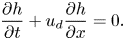 \begin{equation} \frac{\partial h}{\partial t}+ u_d \frac{\partial h}{\partial x}=0. \end{equation}
The dynamic boundary conditions in the tangential and normal directions correspond to
 \begin{gather} \left.\mu_d \frac{\partial u_d}{\partial z}\right\vert_{z=h}=\tau_s, \end{gather}
 \begin{gather}p_d(x,h) = P_a(x,h) - \varPi (x,h) - \sigma\kappa(x,t). \end{gather}
Here,  $\tau _s$ denotes the external shear stress acting on the droplet surface. In (2.5), the pressure inside the droplet, $p_d$, is balanced by the external pressure from the impinging jet $P_a$, the disjoining pressure $\varPi$ and the Laplace pressure $\sigma \kappa$. Note that $\sigma$ is the surface tension coefficient and $\kappa$ is the curvature of the droplet surface, where $\kappa = h_{xx}/(1+h_x^{2})^{3/2}$. Then, in the limit of $\varepsilon \ll 1$, $\kappa$ can be approximated as $h_{xx}$.
Motivated by previous studies of droplet motion (Savva & Kalliadasis Reference Savva and Kalliadasis2011; Pham & Kumar Reference Pham and Kumar2017, Reference Pham and Kumar2019; Charitatos & Kumar Reference Charitatos and Kumar2020), we use a combination of a precursor film and disjoining pressure to model the contact-line dynamics, which is one of two well-established methods used to model contact-line dynamics within the lubrication framework. The alternative method involves specification of a slip law and contact angle that depends on the speed of the contact line. However, because the position of the contact line is not known a priori, this method tends to be computationally challenging. By contrast, the current approach with a precursor film and disjoining pressure eliminates the need for a slip law at the unknown contact line position. Instead, the precursor-film thickness can be chosen to control the spreading speed, whereas the disjoining pressure is set to obtain an equilibrium contact angle. As a consequence, this approach is easier to implement computationally, as the contact-line location can be simply obtained from the droplet profile (Pham & Kumar Reference Pham and Kumar2019).
Therefore, we incorporate a precursor film into our model and introduce disjoining pressure that accounts for the intermolecular interactions near the contact line (Huh & Scriven Reference Huh and Scriven1971; Savva & Kalliadasis Reference Savva and Kalliadasis2011). Note that the precursor film describes a microscopic layer of fluid that exists in front of the contact line, and it has been experimentally observed during droplet spreading. The scale of the precursor film ranges from a few hundred angstroms to a few micrometres (Popescu et al. Reference Popescu, Oshanin, Dietrich and Cazabat2012). To simplify our model, we assume the precursor film begins at the edges of the droplet and extends to cover the entire domain.
The disjoining pressure accounts for the London–van der Waals force between the liquid and the substrate. Here, we use the following form of a two-term disjoining pressure to describe the repulsive and attractive forces of the liquid and the substrate (Schwartz & Eley Reference Schwartz and Eley1998; Leal Reference Leal2007):
 \begin{equation} \varPi=\mathcal{A}\left[\left(\frac{b}{h}\right)^{n}-\left(\frac{b}{h}\right)^{m}\right], \end{equation}
where  $b$ is the thickness of the precursor film. In addition, the Hamaker constant, $\mathcal {A}$, is related to the equilibrium contact angle $\theta _0$ (Schwartz & Eley Reference Schwartz and Eley1998; Leal Reference Leal2007), via
 \begin{equation} \mathcal{A}=\sigma\theta_0^{2}\frac{(n-1)(m-1)}{2b(n-m)}. \end{equation}
Following the previous works, we choose  $m = 2$ and $n = 3$ to provide an appropriate physical description of contact-line motion along with a reasonable computational cost (Espín & Kumar Reference Espín and Kumar2015; Park & Kumar Reference Park and Kumar2017).
Finally, to obtain  $P_a$, we model the external air flow as a far-field irrotational turbulent free jet (Phares et al. Reference Phares, Smedley and Flagan2000), where the characteristic Reynolds number is defined as ${{Re}}=\rho _aU_0d_0/\mu _a$ and is of $O(10^{2})$ or higher. As the position of the nozzle in our analysis is far from the substrate (i.e. $H \gg d_0$), the centreline velocity of the jet is reduced from $U_0$, as the jet entrains more air and widens while approaching the substrate. Hence, we employ the solution of the centreline velocity of the turbulent free jet to describe the decay of centreline velocity (Banks & Chandrasekhara Reference Banks and Chandrasekhara1963; Schlichting & Gersten Reference Schlichting and Gersten2016). The velocity profile of the air flow, $U(x,z)$, is assumed to fit a classic Gaussian distribution (Lunz & Howell Reference Lunz and Howell2018; Ojiako et al. Reference Ojiako, Cimpeanu, Bandulasena, Smith and Tseluiko2020), in good agreement with the experimental measurements (Lemoine, Wolff & Lebouche Reference Lemoine, Wolff and Lebouche1996):
 \begin{equation} \frac{U(x,z)}{U_0}=K_1 \sqrt{\frac{d_0}{H-z}} \exp\left[-\frac{1}{C_1^{2}}\left(\frac{x}{H-z} \right)^{2}\right]. \end{equation}
Here,  $K_1$ is an empirical constant ranging from 2.3 to 2.6, which has been experimentally validated by Banks & Chandrasekhara (Reference Banks and Chandrasekhara1963) for a wide range of $U_0$ (i.e. $7.7\unicode{x2013}128\ {\rm m}\ {\rm s}^{-1}$). For simplicity, we set $K_1=2.5$ in the present study. In addition, $C_1\approx 0.255$, which is obtained based on momentum conservation of the air jet between the nozzle and substrate:
 \begin{equation} \rho_a U_0^{2} d_0=\int_{-\infty}^{\infty} \rho_a U^{2}(x,0) \, {{\rm d}x}. \end{equation}
 As the droplet profile is assumed to be thin in our model, we neglect the effects of the droplet on the air jet itself. In addition, we further approximate the jet profile on the droplet surface as that on the substrate, so that  $U(x,h) \approx U(x,0)$. Finally, the external pressure distribution, $P_a$, can be derived by combining (2.8) and the Bernoulli equation:
 \begin{equation} P_a(x)-P_a(\infty)=\frac{1}{2}\rho_a U_0^{2} K_1^{2} \left(\frac{d_0}{H} \right){\rm{exp}}\left[-\frac{1}{C_1^{2}}\left(\frac{x}{H} \right)^{2}\right]^{2}. \end{equation}
As we model the air pressure distribution with a far-field free turbulent jet, the changes in air pressure due to the presence of the droplet is ignored herein.
In addition to the external pressure, the turbulent jet is also expected to impose shear stress on the droplet surface, which can further deform the droplet via (2.4). Phares et al. (Reference Phares, Smedley and Flagan2000) developed a theoretical framework for estimating the wall shear stress under an impinging jet, which they also validated with experimental measurements. Their results show that the wall shear stress  $\tau _w$ under a two-dimensional jet scales as $\rho _aU_0^{2}{{Re}}^{-1/2} (H/d_0)^{-5/4}$. In § 2.3, we non-dimensionalise $\tau _s$ in (2.4) with $\rho _aU_0^{2}{{Re}}^{-1/2} (H/d_0)^{-5/4}$ and systematically compare the effects of shear stress with those of pressure from the impinging jet.
2.3. Evolution equation
Next, we non-dimensionalise the governing equations and boundary conditions using the following characteristic scales:
 \begin{equation} \left.\begin{gathered} u_{d}^{*}=\frac{u_{d}}{U_s},\quad (x^{*},z^{*})=\left(\frac{x}{L},\frac{z}{\varepsilon L}\right), \quad h^{*}=\frac{h}{\varepsilon L}, \quad b^{*}=\frac{b}{\varepsilon L},\quad t^{*}=\frac{tU_s}{L},\\ P^{*}=\frac{P_a}{\rho_{a} U^{2}_0}, \quad {\rm \pi}^{*}=\frac{\varPi}{\varepsilon\sigma/ L},\quad \tau^{*}_{{s}}=\frac{\tau_{s}\sqrt{{Re}}}{\rho_aU_0^{2}(d_0/H)^{5/4}}, \end{gathered}\right\}\end{equation}
where the asterisk denotes dimensionless variables. Here,  $U_s=\varepsilon ^{3}\sigma /3\mu _d$ is the characteristic capillary speed, which comes from balancing $\mu _d\partial ^{2} u_d/\partial z^{2}$ with $\sigma h_{xxx}$ by combining (2.1) and (2.5). Note that $L$ corresponds to the characteristic half-width of the droplet, which is related to and yet distinct from the initial radius $l$. As further explained in § 2.4, the introduction of $L$ is necessary to initiate the simulations, as $l$ is not known a priori for all droplet sizes but is computed as part of the solution. The plot of the initial droplet radius $l$ as a function of the input parameter $L$ is shown in figure 10 in Appendix A.
By integrating (2.1) and (2.2) and combining with (2.3)–(2.5), we derive the dimensionless evolution equation for  $h^{*}(x^{*}, t^{*})$:
 \begin{align} \frac{\partial h^{*}}{\partial t^{*}}=\frac{\partial}{\partial x^{*}}\left[\left( {{We}} \, \frac{\partial P_a^{*}}{\partial x^{*}}- \frac{\partial^{3} h^{*}}{\partial {x^{*}}^{3}}+{{Bo}}\, \frac{\partial h^{*}}{\partial x^{*}}-\frac{\partial {\rm \pi}^{*}}{\partial x^{*}} \right){{h^{*}}^{3}} - \frac{3}{2}{{We}}\frac{(d_0/H)^{5/4}}{\varepsilon\sqrt{{Re}}}\tau^{*}_s {h^{*}}^{2}\right], \end{align}
with Weber number  ${{We}}=\rho _{a}U_0^{2}L/\varepsilon \sigma$ and Bond number ${{Bo}}=\rho _{d}gL^{2}/\sigma$. Based on the characteristic experimental parameters in Hooshanginejad et al. (Reference Hooshanginejad, Dutcher, Shelley and Lee2020), the magnitude of ${{We}}$ is around $O(10^{1})$ to $O(10^{2})$ whereas $\varepsilon ^{-1}{{Re}}^{-1/2}(d_0/H)^{5/4}$ is approximately $O(10^{-3})$. Therefore, we presently neglect the shear stress term (Kriegsmann et al. Reference Kriegsmann, Miksis and Vanden-Broeck1998; Lunz & Howell Reference Lunz and Howell2018) and further reduce (2.12) to
 \begin{equation} \frac{\partial h^{*}}{\partial t^{*}}=\frac{\partial}{\partial x^{*}}\left[\left( {{We}} \, \frac{\partial P_a^{*}}{\partial x^{*}}- \frac{\partial^{3} h^{*}}{\partial {x^{*}}^{3}}+{{Bo}} \frac{\partial h^{*}}{\partial x^{*}}-\frac{\partial {\rm \pi}^{*}}{\partial x^{*}} \right){{h^{*}}^{3}}\right]. \end{equation}
Henceforth, we drop the asterisks for brevity and assume that all the variables (e.g.  $h$,
$h$,  $x$,
$x$,  $t$ and $P_a$) are dimensionless unless otherwise stated. Note that the physical input parameters (e.g. $L$,
$L$,  $l$,
$l$,  $U_0$, $H$,
$H$,  $d_0$) remain dimensional.
2.4. Numerical method
Equation (2.13) can be solved numerically within the domain  $[-\mathcal {L}, \mathcal {L}]$, with the following boundary conditions:
 \begin{equation} h({\pm}\mathcal{L},t)=b,\quad \frac{\partial h}{\partial {x}}({\pm}\mathcal{L},t)=0. \end{equation}
Combining (2.13) and (2.14a,b), numerical solutions can be obtained by using a fully implicit finite-difference scheme. All spatial derivatives are approximated by second-order centred differences, and the time-integration is performed with the DDASPK iterative solver (Brown, Hindmarsh & Petzold Reference Brown, Hindmarsh and Petzold1994). We set  $\mathcal {L}=5$ with the spatial resolution varying between 200 and 1000 points per unit length for all the simulations reported herein. Note that most of the simulations are run using $200$ nodes per length, as this corresponds to the largest mesh size that produces mesh-independent results (see figure 12 in Appendix C). However, for $U_0 >30 \ \textrm {m}\ \textrm {s}^{-1}$, a finer resolution in time is required to fully capture the droplet deformations, which also decreases the mesh size for numerical stability.
For the initial condition, we first consider a fourth-order polynomial placed between  $x=-1$ and $x=1$, such that the entire liquid profile within the domain is smooth and satisfies (2.14a,b). The shape of the polynomial is determined by fixing the value of the enclosed dimensionless droplet area $A$. The total area in the system is given by $A+2b\mathcal {L}$. Next, we start the simulation with $U_0 = 0\ \textrm {m}\ \textrm {s}^{-1}$ and allow the droplet to relax until it reaches a steady state. We regard this steady-state profile as the initial droplet shape, from which we extract the initial droplet radius $l$. Note that this initial droplet shape is slightly different from the analytical solution for a sessile droplet, due to the presence of a precursor film. If one employs an alternative method (e.g. slip law) to resolve the contact line motion, it would be more straightforward to directly initiate the simulation with a sessile droplet shape with radius $l$. In addition, $t = 0$ in the following discussion refers to the time at which the jet is applied, after the initial droplet relaxation. Finally, at $t=0$, we set the values of $U_0$ and $\alpha$ and run the simulations for $t\sim O(10^{2})$, or until the droplet exhibits a clear behaviour (e.g. splitting). The numerical solutions to the evolution equation are presented in § 3.
2.5. Steady-state solutions
In addition to the numerical solutions to (2.13), we seek analytical solutions of the droplet shape in the steady state. In this limit, the moving-contact-line model is no longer an important factor because the droplet is static. Therefore, we neglect the effects of disjoining pressure and the precursor film in order to obtain the steady-state droplet profile. Based on the above discussion, (2.13) can be simplified as
 \begin{equation} \frac{{\rm d}^{3}h}{{{\rm d} x}^{3}}-{{Bo}}\frac{{\rm d} h}{{\rm d} x}+{{We}}\, \beta (x-\alpha) \exp\left[\frac{-2}{C_1^{2}}\left(\frac{x-\alpha}{H/L}\right)^{2}\right]=0, \end{equation}
where  $\beta =4K_1^{2} d_0 L^{2}/C_1^{2} H^{3}$. We solve (2.15) analytically with the following boundary conditions:
 \begin{equation} h(s_1)=h({-}s_2)=0,\quad \int_{{-}s_2}^{s_1} h \,{{\rm d} x}=A. \end{equation}
Here,  $s_1$ and $s_2$ are the dimensionless contact-line locations that have been normalised by $L$. As the analytical solution to (2.15) can be obtained using a standard symbolic math solver (e.g. Mathematica), we presently do not include the full expression of $h(x)$ in the manuscript for brevity.
Notably,  $s_1$ and $s_2$ are unknown a priori for given dimensionless area $A$. Hence, we simultaneously solve for $s_1$ and $s_2$ by imposing constraints on the contact angles, or
 \begin{equation} -\frac{{\rm d}h}{{\rm d} x}(s_1)=\frac{\theta_1}{\varepsilon}, \quad \frac{{\rm d}h}{{\rm d} x}({-}s_2)=\frac{\theta_2}{\varepsilon}. \end{equation}
Here, we specify the values of  $\theta _1$ and $\theta _2$ based on different physical situations, which will be discussed more explicitly in the next section. Note that the division by $\varepsilon$ stems from non-dimensionalising $\textrm {d}h/{\textrm {d} x}$, which scales with $\varepsilon$ based on the characteristic scales introduced in (2.11).
3. Results
3.1. Droplet behaviours
Previously, Hooshanginejad et al. (Reference Hooshanginejad, Dutcher, Shelley and Lee2020) experimentally studied the dynamics of a partially wetting droplet under an impinging jet. In their experimental results, they divided the observed droplet behaviours into three categories: (i) droplet reaches the equilibrium state, (ii) the droplet moves towards one side and (iii) droplet splits into two. These three droplet regimes are referred to as ‘hanging’, ‘depinning’ and ‘splitting’, respectively. In this section, we reproduce the aforementioned regimes with our lubrication model for varying  $U_0$ and $\alpha$, in comparison with the experiments. We note that given the idealised two-dimensional nature of the model, it is not reasonable to quantitatively match the results of the simulations and experiments for the same parameter values. Instead, we focus on demonstrating that the simulations can qualitatively reproduce all three droplet behaviours and exhibit similar time scales. Hence, we fix the values of the initial droplet radius, $l$ and $\alpha$, but use slightly different $U_0$ from the experiments to simulate the observed droplet motion. Specifically, we let $l=7.7 \ \textrm {{mm}}$ (corresponding to $200\ \mathrm {\mu } \textrm {l}$ in the experiments), $\mathcal {A}=1000$, $b=10^{-3}$ and $A=0.5$. Based on the current values of $\mathcal {A}$ and $b$, the equilibrium contact angle $\theta _0$ is equal to $30^{\circ }$, which matches the experimental observation by Hooshanginejad et al. (Reference Hooshanginejad, Dutcher, Shelley and Lee2020). The simulation results are presented in figures 2–4, along with the images from the corresponding experiments. We also include the simulation videos of the evolving droplet shapes as supplementary material available at https://doi.org/10.1017/jfm.2022.450.

Figure 2. (a) Time-sequential images of the droplet hanging regime from the simulation and the experiment at dimensional times,  $t=0,34,130\ \textrm {{ms}}$. (i) The simulation results are for a droplet of $l=7.7\ \textrm {{mm}}$ under a centred jet $(\alpha =0)$ with the jet speed $U_0=9.8\ \textrm {{m}}\ \textrm {s}^{-1}$. (ii) The experimental results correspond to $l=7.7 \ \textrm {{mm}}\ (200\ \mathrm {\mu } \textrm {l})$, $\alpha =0$ and $U_0=6.6 \ \textrm {{m}}\ \textrm {s}^{-1}$. (b) We plot $p_d(x,h)$, the internal pressure distribution at $z=h(x,t)$, as a function of the normalised horizontal location, $x_N=(2x-s_1+s_2)/(s_2+s_1)$, at different time instants; $p_d(x,h)$ corresponding to the three time instants in (i) are marked as solid black lines.

Figure 3. (a) Time-sequential images of the splitting regime from the simulation and the experiment at dimensional times,  $t=0,170,300\ \textrm {{ms}}$. (i) The simulation results are for a droplet of $l=7.7\ \textrm {{mm}}$ under a centred jet $(\alpha =0)$ with the jet speed $U_0=19\ \textrm {{m}}\ \textrm {s}^{-1}$. (ii) The experimental results correspond to $l=7.7 \ \textrm {{mm}}\ (200 \ \mathrm {\mu } \textrm {l})$, $\alpha =0$ and $U_0=13.4\ \textrm {{m}}\ \textrm {s}^{-1}$. (b) We plot $p_d(x,h)$, the internal pressure distribution at $z=h(x,t)$, as a function of the normalised horizontal location, $x_N$, at different time instants; $p_d(x,h)$ corresponding to the three time instants in (i) are marked as solid black lines.

Figure 4. (a) Time-sequential images of the depinning regime from the simulation and the experiment at dimensional times,  $t=0,225,375\ \textrm {{ms}}$. (i) The simulation results are for a droplet of $l=7.7\ \textrm {{mm}}$ under an off-centred jet $(\alpha =-0.53)$ with the jet speed $U_0=17 \ \textrm {{m}}\ \textrm {s}^{-1}$. (ii) The experimental results correspond to $l=7.7 \ \textrm {{mm}}\ (200 \ \mathrm {\mu } \textrm {l})$, $\alpha =-0.53$ and $U_0=15 \ \textrm {{m}}\ \textrm {s}^{-1}$. (b) We plot $p_d(x,h)$, the internal pressure distribution at $z=h(x,t)$, as a function of $x_N$ for increasing time; $p_d(x,h)$ corresponding to the three time instants in (i) are marked as solid black lines.
Figure 2(a) shows time-sequential images of droplet ‘hanging’ for  $\alpha =0$ from the simulation (left) and the experiment (right). As the jet speed in both the experiment ( $U_0=6.6 \ \textrm {{m}}\ \textrm {s}^{-1}$) and the simulation ( $U_0=9.8\ \textrm {{m}}\ \textrm {s}^{-1}$) is relatively low, the droplet deforms only slightly near the centre, until it reaches an equilibrium state. Note that, in the experiments, the droplet continues to oscillate about the equilibrium shape, which is not captured in the current model due to the neglect of the droplet inertia as well as the fluctuations in the free jet.
To gain understanding of the underlying physics, we plot the dimensionless internal pressure of the droplet  $p_d(z=h)$ over time in figure 2(b). Here, the horizontal axis $x_N$ is the normalised location of the droplet contact line, i.e. $x_N=(2x-s_1+s_2)/(s_2+s_1)$, so that the droplet is bounded within $[-1,1]$. When the jet is first applied, $p_d$ increases near the centre but gradually flattens due to the balance of the external, hydrostatic and capillary pressures. Then, when the dimensional time reaches $130\ \textrm {{ms}}$, $p_d$ becomes uniform throughout, which coincides with the new equilibrium state of the droplet. The value of constant $p_d$ at the final time is higher than that at the initial time (i.e. $U_0 = 0\ \textrm {{m}}\ \textrm {s}^{-1}$), as the overall droplet shape has changed due to the external flow. However, it is important to point out the existence of a large capillary pressure gradient near the contact line that is balanced by a large disjoining pressure gradient, so the total pressure is only approximately constant.
To consider the case of droplet splitting, we increase the jet speed over the threshold ( $U_0 > U_{cr}$), whereas the droplet size and $\alpha$ remain unchanged from the hanging case. As shown in figure 3(a), the droplet continues thinning at the centre due to the strong air jet in both the experiment $(U_0=13.4\ \textrm {{m}}\ \textrm {s}^{-1}$) and the simulation $(U_0=19\ \textrm {{m}}\ \textrm {s}^{-1}$), in clear departure from the ‘hanging’ regime. Then, at around $300\ \textrm {{ms}}$, the droplet breaks up and forms two residual droplets. This new droplet outcome is made clear in the evolution of the internal pressure $p_d$. As shown in figure 3(b), no equilibrium state (i.e. uniform $p_d$) is reached in this simulation, as the pressure continues to increase near the centre over time. In particular, near the time of droplet rupture ( $300\ \textrm {{ms}}$), the droplet height near the centre is close to that of the precursor film $b$, allowing the disjoining pressure to become dominant (Lenz & Kumar Reference Lenz and Kumar2007). Then, the pressure difference between $x_N=0$ and near the edges ensures that the fluid continues to drain from the centre, which, in turn, enhances the pressure difference and eventually causes the droplet to rupture.
In figure 4, we consider the case with  $\alpha =-0.53$ that induces droplet depinning with a jet speed of $U_0=15\ \textrm {{m}}\ \textrm {s}^{-1}$ in the experiment and $U_0=17\ \textrm {{m}}\ \textrm {s}^{-1}$ in the simulation. When the jet is first applied, the droplet tends to spread out, with the contact line advancing from its initial position on both sides. Shortly following the initial spreading, the droplet deforms asymmetrically and gradually moves away from the nozzle, as illustrated in figure 4(a). Specifically, the right edge (further from the nozzle) keeps advancing, whereas the contact line on the left side changes its direction of motion and starts to recede, so that the droplet as a whole moves to the right away from the nozzle.
This droplet dynamics can be understood by examining the dimensionless internal pressure in figure 4(b). Namely,  $p_d$ near the left contact line increases over time and overcomes the large pressure from the nozzle. Around $225 \ \textrm {{ms}}$, the pressure monotonically decreases from the left to right edges, which is followed by the droplet depinning (see figure 4a). Then, at $375 \ \textrm {{ms}}$, the droplet is shown to have further dislodged away from the nozzle. However, the droplet appears to be more asymmetrical in the experiment than in the simulation, due to the continuous oscillations and the lateral flow of air in the experiment that are not captured by our model. Hence, the two requisite conditions for droplet depinning are (i) $U_0$ that is not large enough to cause splitting and (ii) sufficient asymmetry in the internal pressure set by $\alpha \ne 0$, so that the resulting pressure distribution is either monotonically increasing or decreasing from one side of the droplet to the other. Note that the direction of droplet depinning and the sign of the pressure gradient will reverse for $\alpha >0$.
3.2. The case of a centred jet
In this section, we consider the case of a centred jet ( $\alpha =0$) and identify the velocity threshold for droplet splitting ( $U_{cr}$), by combining the numerical simulations and analytical solutions. For the simulations, we set $\mathcal {A}=1000$, $b=10^{-3}$ and $A=1$. Then, to obtain $U_{cr}$, we gradually increase the jet speed $U_0$ with an increment of $1 \ \textrm {{m}}\ \textrm {{s}}^{-1}$ for given $L$ (or $l$) until the droplet behaviour transitions from ‘hanging’ to ‘splitting’. In figure 5, the maximum $U_0$ for droplet hanging is marked with an ‘x’, whereas the minimum $U_0$ for droplet splitting is shown with a filled square. Then, $U_{cr}$ is bounded within these two marked values of $U_0$ and is shown as a grey-shaded region in figure 5. Note that resultant $U_{cr}$ decreases with $l$, which is qualitatively consistent with the experimental observations of Hooshanginejad et al. (Reference Hooshanginejad, Dutcher, Shelley and Lee2020). In particular, $U_{cr}$ appears to plateau to a constant value just above $15\ \textrm {{m}}\ \textrm {{s}}^{-1}$ for large $l$ (i.e. $l > 5 \ \textrm {{mm}}$), which sits outside the available experimental range.

Figure 5. Plot of the critical jet speed for droplet splitting  $U_{cr}$ versus $l$ from the numerical simulations (grey area), the steady-state prediction that accounts for the contact line motion (solid blue line) and the steady-state solution with a pinned contact line by Hooshanginejad et al. (Reference Hooshanginejad, Dutcher, Shelley and Lee2020) (dashed red line). For the simulation results, we note the droplet splitting behaviour with a filled square and the hanging regime with a cross, which provide the upper and lower bounds for $U_{cr}$.
To rationalise the relationship between  $U_{cr}$ and $l$, we consider the steady-state solution described in § 2.5. When $U_0 = U_{cr}$, we assume that $h(x)$ must satisfy the splitting criterion of $h(x=0)=0$. Hence, $U_{cr}$ is equivalent to the maximum jet speed at which the droplet reaches equilibrium. However, $h(x)$ involves an additional unknown, $s_1=s_2=s$, which is the dimensionless position of the contact line. In order to compute $s$ as part of the solution, we impose $\theta _1=\theta _2 = \theta _0$ in (2.17a,b) for simplicity, because the dynamic contact angle for droplet spreading must be equal to (or greater than) the equilibrium contact angle, $\theta _0$. Finally, to extract $U_{cr}$, we start with the initial guess of $s=1$ and compute $h(x)$, after we set $L$ and $A=1$. By imposing $h(x=0)=0$, we solve for $U_{cr}$ (or, equivalently, ${{We}}_{cr}$), as shown in (B1). Then, if the resultant $h(x)$ does not meet the contact-angle condition, we increase $s$ with an increment of $0.001$ and repeat the process, until $\theta _1=\theta _2 = \theta _0$. The resultant $U_{cr}$ from the analytical solutions is included in figure 5 as a solid line, and it matches the numerical simulations with no additional fitting parameters beyond previously described assumptions and approximations. This agreement between the simulations and theory helps validate our splitting criterion and the contact-angle condition, as well as the neglect of the disjoining pressure in the current physical regime.
The decrease of  $U_{cr}$ with $l$ in both the numerical and steady-state solutions can be understood by considering the dominant physical effects at play. For small $l$, it is reasonable to assume that the droplet dynamics are set by the competition between the capillary pressure and the external air pressure, while the hydrostatic pressure is negligible. In fact, the initial pressure inside small droplets must scale as $l^{-1}$. Hence, it would require a larger external pressure to overcome this capillary pressure and split the droplet into two, which corresponds to $U_{cr}$ decreasing with increasing $l$. Then, for large droplets, we expect the droplet dynamics to be governed by the balance between the hydrostatic pressure and the external airflow, which no longer explicitly depends on $l$. The transition from ‘small’ to ‘large’ droplets can be estimated as when the droplet height becomes constrained by the capillary length, or $h_m = 2\sqrt {\sigma /(\rho g)}\sin {(\theta _0/2)}\approx 1.4\ \textrm {mm}$ (de Gennes, Brochard-Wyart & Quéré Reference de Gennes, Brochard-Wyart and Quéré2004). Assuming a simple circular segment as the initial droplet shape, the transitional droplet size is given by $l = h_m\sin {\theta _0}/(1-\cos {\theta _0})\approx 5.3\ \textrm {mm}$, which reasonably matches the transition to constant $U_{cr}$ in figure 5.
Furthermore, we perform an asymptotic analysis to explain this plateau in  $U_{cr}$ for large $l$. We take the analytical solution for ${{We}}_{cr}$ in the limit of ${{\sqrt {Bo}}} s \rightarrow \infty$, with the details shown in Appendix B. Note that the limit of large ${{\sqrt {Bo}}}s$, or large $L$, is equivalent to the limit of large $l$, as there is a clear monotonic relationship between $l$ and $L$ for given dimensionless area, $A$ (see Appendix A). Finally, the resultant ${{We}}_{cr}$ in the asymptotic limit is given by
 \begin{equation} {{We}}_{cr}\propto\frac{\sqrt{{Bo}}}{s(d_0/L)}, \end{equation}
where  $s$ is shown to scale linearly with $L$ for large $L$ (see Appendix B), such that $s(d_0/L)$ is a constant. Therefore, in the large-droplet limit, ${{We}}_{cr}$ is shown to scale with $\sqrt {Bo}$, and $U_{cr}$ becomes independent of the droplet size, consistent with the simulations. Physically speaking, this balance of ${{We}}_{cr}$ and $\sqrt {Bo}$ confirms that as $l$ is increased, the external air pressure is indeed mostly balanced by the hydrostatic pressure inside the droplet.
Figure 5 also includes  $U_{cr}$ based on the steady-state solution with a pinned contact line (Hooshanginejad et al. Reference Hooshanginejad, Dutcher, Shelley and Lee2020). In general, pinning the contact line is expected to increase the critical jet speed required for splitting, as the droplet can split only by draining from the centre and not by spreading of the droplet caused by a change of the contact-line locations. This explains why the pinned contact-line model exhibits a larger $U_{cr}$ compared with the moving contact-line model for $l< 5 \ \textrm {mm}$. However, this physical picture breaks down for $l> 5 \ \textrm {mm}$, as $U_{cr}$ with the fixed contact line continues to decrease with $l$ with no plateau, distinct from the moving contact-line simulations and theory. This discrepancy is caused by the fact that the contact line is pinned at the location given by the radius of a circular cap with the equivalent area. Note that a circular cap as the initial droplet geometry is valid for small droplets (i.e. $l< 5 \ \textrm {mm}$) but becomes problematic for large droplets (i.e. $l> 5\ \textrm {mm}$) that form puddles under gravity. Hence, for $l> 5 \ \textrm {mm}$, the model by Hooshanginejad et al. (Reference Hooshanginejad, Dutcher, Shelley and Lee2020) tends to pin the contact line at a smaller radius than where the contact line would initially be. This likely causes larger interfacial deformations near the contact line and larger pressure gradients necessary to drive the draining flow from the centre towards the edge, leading to a decrease in $U_{cr}$.
3.3. Case of an off-centred jet
Next, we consider the case of an off-centred jet and identify the droplet behaviours under different  $U_0$ and $\alpha$ for given $l$. For $l=4.9\ \textrm {{mm}}$ ( $50\ \mathrm {\mu }\textrm {{l}}$ in the experiment) and $7.7 \ \textrm {{mm}}$ ( $200\ \mathrm {\mu }\textrm {{l}}$ in the experiment), we set $\mathcal {A}=1000$, $b=10^{-3}$, $A=1$ and gradually change $U_0$ (with an increment of $1\ \textrm {{m}}\ \textrm {{s}}^{-1}$) and $\alpha$ (with an increment of 0.05) in the simulations. The resulting droplet regimes are summarised in the $\alpha -U_0$ phase diagrams in figure 6, with ‘x’ marking the ‘hanging’ regime, a triangle denoting depinning and a square indicating splitting. Note that figures 6(b) and 6(d) show corresponding phase diagrams from the experimental data of Hooshanginejad et al. (Reference Hooshanginejad, Dutcher, Shelley and Lee2020).

Figure 6. Phase diagrams summarising the outcomes of the droplet dynamics with varying  $U_0$ and $\alpha$, for (a) $l=4.9 \ \textrm {{mm}}$ and (c) $l=7.7 \ \textrm {{mm}}$. Three regimes are identified: droplet splitting (square), depinning (triangle) and hanging (cross). The corresponding experimental results for (b) $l=4.9 \ \textrm {{mm}}$ and (d) $l=7.7 \ \textrm {{mm}}$, respectively.
The phase diagrams based on the simulations (figures 6a and 6c) clearly exhibit three regimes: hanging, depinning and splitting, in a manner that is qualitatively consistent with the experiments. For both values of  $l$, the critical jet speed for droplet splitting increases with increasing $\alpha$, whereas the transitional velocity from hanging to depinning decreases with $\alpha$. Hence, the range of $U_0$ over which depinning occurs increases with $\alpha$ for both droplet sizes. In the case of $l=7.7 \ \textrm {{mm}}$ only, we observe no droplet depinning for $\alpha <0.1$, whereas we observe droplet depinning for all non-zero values of $\alpha$ in the case of $l=4.9 \ \textrm {{mm}}$. In Appendix D, we also consider the droplet behaviours in the larger range of $\alpha$, which shows the elimination of droplet splitting for $\alpha >1$ (see figure 13).
To further investigate this apparent suppression of depinning for large  $l$, we conduct additional simulations for $l$ ranging from $2.4\ \textrm {{mm}}$ to $12.8 \ \textrm {{mm}}$. The results are summarised in a series of phase diagrams in figure 7(a). Similar to the case of $l=4.9 \ \textrm {{mm}}$, droplet depinning is observed for all $\alpha >0$ at $l=2.4 \ \textrm {{mm}}$ (see figures 7a–7i), and the depinning region gradually increases with $\alpha$. For larger droplets, depinning is suppressed below some threshold $\alpha$, whose value grows with $l$. We refer to this threshold as $\alpha _{sup}$ and mark its position with a vertical dashed line in the $\alpha -U_0$ phase diagrams in figure 7(a). Then, as shown in figure 7(b), $\alpha _{sup}$ is equal to zero for small droplets, or $l<5\ \textrm {{mm}}$, and then monotonically increases with $l$ for $l>5 \ \textrm {{mm}}$.
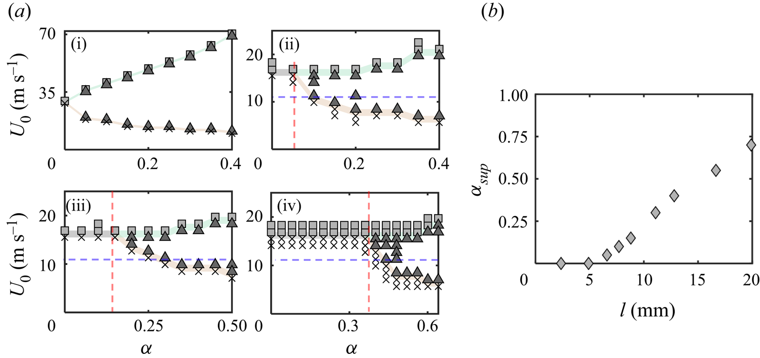
Figure 7. (a) The numerical  $\alpha - U_0$ phase diagrams for the following droplet sizes: (i) $l=2.4\ \textrm {{mm}}$, (ii) $l=6.6\ \textrm {{mm}}$, (iii) $l=8.8\ \textrm {{mm}}$ and (iv) $l=12.8\ \textrm {{mm}}$, with splitting (square), depinning (triangle) and hanging (cross) regimes. Vertical and horizontal dashed lines indicate the values of $\alpha _{sup}$ and $\alpha _{cr}$, respectively. (b) The value of $\alpha _{sup}$ (below which depinning is suppressed) is computed from the simulations and plotted as a function of $l$.
$l$.
The physical mechanism behind depinning suppression can be understood by comparing the size of the droplet  $l$ and the size of the external pressure distribution. We define the characteristic half-width of the external pressure distribution as $\delta$. The requirement for droplet depinning is a large enough internal pressure difference between the two edges of the droplet to drive the fluid from one side to the other. However, for small $\alpha$, if the size of the droplet is greater than the size of the external pressure distribution (i.e. $l >\delta$), the internal pressure near the contact line is not influenced by the air jet and is unable to meet this requirement.
Going back to figure 7(a), there exists a critical  $\alpha$ (denoted as $\alpha _{cr}$) that separates the hanging and depinning regimes at fixed $U_0$, which is shown with a horizontal dashed line in the phase diagrams for $U_0=11\ \textrm {m}\ \textrm {s}^{-1}$. This allows us to investigate the relationship between $\alpha _{cr}$ and $l$ by combining the simulations and steady-state solutions. Note that $\alpha _{sup}$ is the minimum of $\alpha _{cr}$ for given $l$. In the simulation, we set $l$ and $U_0=11\ \textrm {m}\ \textrm {s}^{-1}$, in addition to $\mathcal {A}=1000$, $b=10^{-3}$ and $A=1$. We obtain $\alpha _{cr}$ by gradually increasing $\alpha$ with an increment of $0.005$ and identifying the droplet behaviour until it transitions from hanging to depinning. As shown in figure 8, we note the maximum value of $\alpha$ for droplet hanging (marked with an ‘x’) and the minimum $\alpha$ for droplet depinning (a triangle), respectively. Then, $\alpha _{cr}$ from the simulations is bounded within the two values of $\alpha$ for varying $l$, which is shown as a grey region in figure 8.

Figure 8. Simulation results (grey area) and theoretical predictions (dashed lines) of  $\alpha _{cr}$ at $U_0=11\ \textrm {m}\ \textrm {s}^{-1}$ and for varying $l$, whereas we set the vertical location of the nozzle to be: (a) $H=20\ \textrm {{mm}}$, (b) $H=30\ \textrm {{mm}}$ and (c) $H=40\ \textrm {{mm}}$, respectively. The different dashed lines (coloured from dark to light green) correspond to the different values of $\lambda =1$, $1.1$, $1.2$ and $1.3$, which determine the location of the contact line prior to receding relative to the initial position of the droplet's centre. The inset in (a) shows the zoomed-in plot of the region highlighted in the main panel.
We also obtain the theoretical prediction for  $\alpha _{cr}$ based on the steady-state solutions of $h(x)$ discussed in § 2.5. Namely, we seek a steady droplet profile with $A=1$ that satisfies the onset of depinning, depicted in figure 9(a). Here, the onset of depinning corresponds to the formation of the maximum contact angle ( $\theta _2$) on the advancing contact line and the minimum contact angle ( $\theta _1$) on the receding side (Hooshanginejad & Lee Reference Hooshanginejad and Lee2017, Reference Hooshanginejad and Lee2022). Note that the current configuration dictates that the droplet depins from right to left, which is observed experimentally and numerically for $\alpha >0$ only. Based on the simulation results, we set $\theta _{2}=30^{\circ }$ and $\theta _{1}=25^{\circ }$ in (2.17a,b). In addition, we set $s_1=\lambda$ as a reference point, where $\lambda$ is a dimensionless position of the receding contact line at the time of depinning relative to the initial position of the droplet's centre. Fixing $\lambda$ and, thereby, the droplet's centre at $t=0$ is important to define $\alpha$, as $\alpha$ in the experiments corresponds to the dimensionless distance between the position of the nozzle and the droplet's centre prior to the jet application. Finally, for given $l$,
$l$,  $U_0$ and $\lambda$, we compute $\alpha _{cr}$ by performing two nested iterations. First, to solve for $h(x)$ at the onset of depinning, we set $\alpha$ and incrementally increase $s_2$ from $1$, until the contact angle conditions are met. Next, if no such steady-state solution exists at given $\alpha$, we vary $\alpha$ and repeat the process until the solution is found, which eventually leads to $\alpha _{cr}$.

Figure 9. (a) The schematic of the droplet at the onset of droplet depinning. (b) The three schematics describe the qualitative relationship between the size of the jet ( $\delta$) for different droplet sizes, $l$: (i) $\delta >l$, (ii) $\delta \approx l$ and (iii) $\delta < l$.
Both the simulation and theoretical results in figure 8(a) demonstrate that  $\alpha _{cr}$ exhibits a convex behaviour with varying $l$ at $U_0=11\ \textrm {m}\ \textrm {s}^{-1}$. The qualitative match between the simulation and theory confirms the validity of the simple depinning criterion based on contact angles. Notably, the general trend in theoretical $\alpha _{cr}$ versus $l$ is independent of the specific value of $\lambda$. However, at $\lambda = 1$, $\alpha _{cr}$ becomes negative for some range of $l$, which is outside of the reasonable range for a droplet depinning from right to left. This implies that the initial position of the droplet's centre we have arbitrarily set is incorrect and needs to be shifted further left. Consistent with this picture, when we increase $\lambda$ to $1.2$ and move the droplet's centre further from the droplet's right edge, $\alpha _{cr}$ is no longer negative and closely matches the simulation results. Hence, in order to correctly capture $\alpha _{cr}(l)$ at given $U_0$, the position of the receding contact line at the time of depinning needs to be adjusted until $\alpha _{cr}$ is no longer negative.
The key physical feature of this convex behaviour can be captured by again considering the droplet size  $l$, relative to the characteristic half-width of the external jet $\delta$. Figure 9(b) illustrates the comparison of three different droplet sizes under a fixed external pressure distribution. When $l < \delta$, a large enough $\alpha$ is necessary for depinning, because the pressure variation near the centre of the jet is relatively small. Hence, for the internal pressure to have a large enough difference between the contact-line positions, the droplet needs to be exposed to the jet away from its centre (see figure 9b-i). Similarly, the case of $l >\delta$ also requires large $\alpha$ to ensure that there is sufficient asymmetry in the internal pressure, as illustrated in figure 9(b-iii). Finally, when $l \approx \delta$ (see figure 9b-ii), relatively small $\alpha$ can cause a sufficient internal pressure difference for droplet depinning.
Based on this physical picture, we hypothesise that an increase in  $\delta$ should lead to larger $l$ at which $\alpha _{cr}(l)$ reaches a minimum. To test this idea, we increase the value of $\delta$ by increasing the nozzle height $H$ and reproduce the plot of $\alpha _{cr}(l)$ for $H=30 \ \textrm {mm}$ and ${H=40\ \textrm {mm}}$, respectively. Figures 8(b) and 8(c) shows that the value of $l$ where $\alpha _{cr}$ is the minimum increases as $H$ is increased, confirming our hypothesis.
4. Summary and conclusions
In summary, we theoretically analyse the dynamics of partially wetting droplets under an impinging jet based on a two-dimensional lubrication model that incorporates a moving contact line. The numerical simulations reproduce some of the droplet behaviours observed in the experiments by Hooshanginejad et al. (Reference Hooshanginejad, Dutcher, Shelley and Lee2020): droplet hanging, splitting and depinning away from the jet, for the varying jet strength ( $U_0$) and position ( $\alpha$). The three regimes are summarised in a phase diagram as a function of $U_0$ and $\alpha$, for the given droplet diameter $l$, in qualitative agreement with the experiments. The simulations also provide the evolution of the droplet internal pressure corresponding to each droplet behaviour. Specifically, the internal pressure distribution (i) becomes uniform throughout (hanging), (ii) peaks at the position of the jet impingement (splitting) and (iii) monotonically increases or decreases (depinning), respectively. In addition to capturing the droplet regimes, the numerical simulations and the analytical steady-state solutions are able to qualitatively reproduce the critical jet speed for droplet splitting ( $U_{cr}$), which plateaus in the limit of large $l$. By applying an asymptotic analysis to the steady-state solutions, we demonstrate that this plateau stems from the balance of the external air pressure and the hydrostatic pressure as $l$ increases. We also observe that $U_{cr}$ no longer plateaus but continues to decrease when the contact line is pinned.
Furthermore, when the jet is applied off-centre (i.e.  $\alpha \ne 0$), our simulations show that the droplet depinning is suppressed below a certain threshold value of $\alpha$, consistent with the experimental observations. This threshold $\alpha _{sup}$ is equal to zero for small droplets and monotonically increases with $l$. The transition to non-zero $\alpha _{sup}$ occurs as the size of the droplet becomes greater than the characteristic width $\delta$ of the external jet. Finally, by combining the numerical simulations and steady-state solutions, we obtain a theoretical prediction of $\alpha _{cr}$, which separates the hanging and depinning regimes at fixed $U_0$. The results show that $\alpha _{cr}$ exhibits a convex behaviour with varying $l$.
$l$.
Our two-dimensional lubrication model successfully captures some macroscopic behaviours of a partially wetting droplet under a turbulent jet. Distinct from the original lubrication model by Hooshanginejad et al. (Reference Hooshanginejad, Dutcher, Shelley and Lee2020), the current analysis is able to describe the motion of the contact line and reproduce the depinning regime, by incorporating a precursor film and disjoining pressure. However, the model incorporates a number of major assumptions that could be improved upon in future studies. For example, we will simulate experimentally observed oscillations of the droplet, by including the effects of droplet inertia and fluctuations in the jet. We also plan to expand our lubrication model to a three-dimensional system. In the splitting regime, the current simulations consistently show the emergence of a satellite droplet, whose size depends on  $U_0$ and $l$. However, it is unclear if this observation is physically valid or is related to the two-dimensional nature of the model. Hence, the three-dimensional model and additional experiments may be important in quantifying the generation of secondary droplets. Furthermore, we plan to combine the experiments and theory to investigate the potential changes in the droplet behaviour for varying wettability or by applying the jet at an angle.
Supplementary movies
Supplementary movies are available at https://doi.org/10.1017/jfm.2022.450.
Acknowledgements
S.L. and Z.-Y.C. are partly funded by the National Science Foundation (CBET-2032354 and CMMI-2042740). S.K. acknowledges partial support from the National Science Foundation under Grant No. CBET-1935968.
Funding
We thank Dr V. Charitatos for fruitful discussions and Mr Z. Kujala for careful reading of our manuscript.
Declaration of interests
The authors report no conflict of interest.
Appendix A. The relation between  $l$ and $L$


In order to obtain the initial droplet half-width  $l$, we start the simulation with $U_0 = 0$ for given $L$ and allow the droplet to relax until it reaches a steady state. We regard this steady-state profile as the initial droplet shape, from which we extract the initial droplet half-width, $l$. The relation between $l$ and $L$ is shown in figure 10 for the case of $A=1$ (blue line) and $A=0.5$ (red line), respectively.

Figure 10. Relationship between the droplet half-width,  $l$, and the input length scale, $L$, for $A=1$ (blue line) and $A=0.5$ (red line).
Appendix B. Asymptotic analysis: critical jet speed
Consistent with the splitting criterion by Hooshanginejad et al. (Reference Hooshanginejad, Dutcher, Shelley and Lee2020), we define the critical Weber number  ${{We}}_{cr}$ as the threshold for droplet splitting, by taking the analytical steady-state solution $h(x)$ for $\alpha =0$ and then setting $h(x=0)=0$:
 \begin{align}
{{We}}_{cr}&=\frac{-A\sqrt{2/{\rm \pi}}}{C_1(d_0/L) K_1^{2}} \nonumber\\
&\quad \times\frac{{{Bo}}\left(1-{\rm e}^{{-}4jk}
\right)^{2}}
{\left[\begin{array}{ll}
{\rm e}^{j^{2}}{\rm{erf}}(j)\left[{\rm
e}^{{-}4jk}(1+2jk)+(2jk-1)
\right]+{\rm{erf}}(k)\left(1-2{\rm e}^{{-}2jk} \right)\\
+\,{\rm e}^{j^{2}}\left[\begin{array}{ll} {\rm{erf}}(j\!-\!k){\rm
e}^{{-}2jk}\left(1\!-\!{\rm e}^{{-}2jk}(1\!+\!2jk) \right)\\
-{\rm{erf}}(j+k)\left((2jk-1)+{\rm e}^{{-}2jk} \right)
\end{array}\right]\qquad\qquad\end{array}\right]}.
\end{align}
\begin{align}
{{We}}_{cr}&=\frac{-A\sqrt{2/{\rm \pi}}}{C_1(d_0/L) K_1^{2}} \nonumber\\
&\quad \times\frac{{{Bo}}\left(1-{\rm e}^{{-}4jk}
\right)^{2}}
{\left[\begin{array}{ll}
{\rm e}^{j^{2}}{\rm{erf}}(j)\left[{\rm
e}^{{-}4jk}(1+2jk)+(2jk-1)
\right]+{\rm{erf}}(k)\left(1-2{\rm e}^{{-}2jk} \right)\\
+\,{\rm e}^{j^{2}}\left[\begin{array}{ll} {\rm{erf}}(j\!-\!k){\rm
e}^{{-}2jk}\left(1\!-\!{\rm e}^{{-}2jk}(1\!+\!2jk) \right)\\
-{\rm{erf}}(j+k)\left((2jk-1)+{\rm e}^{{-}2jk} \right)
\end{array}\right]\qquad\qquad\end{array}\right]}.
\end{align}Here, for simplicity, we have defined
 \begin{equation} j\equiv \frac{\sqrt{{{Bo}}}sC_1}{2\sqrt 2}\left(\frac{H}{L}\right);\quad k\equiv \frac{\sqrt 2 s}{C_1}\left(\frac{H}{L}\right), \end{equation}
such that  $2jk=\sqrt {{Bo}}s$. We note that $j$ is a constant independent of $L$, whose value is approximately equal to $0.661$. On the other hand, $k$ can be rearranged as
 \begin{equation} k\equiv \frac{\sqrt 2}{C_1}\frac{\sqrt{{{Bo}}}s}{\sqrt{{{Bo}}_H}} \approx 0.756 \sqrt{{{Bo}}}s, \end{equation}
where  ${{Bo}}_H=\rho _d gH^{2}/\sigma$. Therefore, it is reasonable to assume that the limit of $\sqrt {{{Bo}}}s\gg 1$ is equivalent to $k \gg 1$. Next, we expand the error functions in the limit of $k \gg 1$, so that ${{We}}_{cr}$ becomes
 \begin{align}
{{We}}_{cr}&\approx\frac{-A\sqrt{2/{\rm \pi}}}{C_1(d_0/L)
K_1^{2}}\nonumber\\
&\quad \times\frac{{{Bo}}\left(1-{\rm e}^{{-}4jk}
\right)^{2}}
{\left[\begin{array}{@{}ll@{}}
{\rm e}^{j^{2}}{\rm{erf}}(j)\left[{\rm e}^{{-}4jk}(1+2jk)+(2jk-1) \right]\\
+\left\{1- \dfrac{{\rm e}^{{-}k^{2}}}{\sqrt {\rm \pi}k}+ {\rm{h.o.t.}}
\right\}\left(1-2{\rm e}^{{-}2jk} \right)\\
+\,{\rm e}^{j^{2}}\left[\begin{array}{l}\left\{1- \dfrac{{\rm
e}^{(j-k)^{2}}}{\sqrt {\rm \pi}k}+ {\rm{h.o.t.}} \right\}{\rm
e}^{{-}2jk}\left(1-{\rm e}^{{-}2jk}(1+2jk) \right)\\
-\left\{1- \dfrac{{\rm e}^{(j+k)^{2}}}{\sqrt {\rm \pi}k}+
{\rm{h.o.t.}} \right\}\left((2jk-1)+{\rm e}^{{-}2jk}
\right)\end{array}\right]\end{array}\right]},
\end{align}
\begin{align}
{{We}}_{cr}&\approx\frac{-A\sqrt{2/{\rm \pi}}}{C_1(d_0/L)
K_1^{2}}\nonumber\\
&\quad \times\frac{{{Bo}}\left(1-{\rm e}^{{-}4jk}
\right)^{2}}
{\left[\begin{array}{@{}ll@{}}
{\rm e}^{j^{2}}{\rm{erf}}(j)\left[{\rm e}^{{-}4jk}(1+2jk)+(2jk-1) \right]\\
+\left\{1- \dfrac{{\rm e}^{{-}k^{2}}}{\sqrt {\rm \pi}k}+ {\rm{h.o.t.}}
\right\}\left(1-2{\rm e}^{{-}2jk} \right)\\
+\,{\rm e}^{j^{2}}\left[\begin{array}{l}\left\{1- \dfrac{{\rm
e}^{(j-k)^{2}}}{\sqrt {\rm \pi}k}+ {\rm{h.o.t.}} \right\}{\rm
e}^{{-}2jk}\left(1-{\rm e}^{{-}2jk}(1+2jk) \right)\\
-\left\{1- \dfrac{{\rm e}^{(j+k)^{2}}}{\sqrt {\rm \pi}k}+
{\rm{h.o.t.}} \right\}\left((2jk-1)+{\rm e}^{{-}2jk}
\right)\end{array}\right]\end{array}\right]},
\end{align}
where ‘h.o.t.’ denotes the higher-order terms. Then, under the limit of  $\sqrt {{{Bo}}}s\gg 1$ (i.e. $k\gg 1$ and $2jk\gg 1$), ${{We}}_{cr}$ reduces to
 \begin{equation} {{We}}_{cr}\approx\frac{A\sqrt{2/{\rm \pi}}}{C_1(d_0/L) K_1^{2}} \left[\frac{Bo}{{\rm e}^{j^{2}}(1-{\rm{erf}}(j))\sqrt{{{Bo}}}s}\right], \end{equation}
where  $\textrm {e}^{j^{2}}(1-\textrm {{erf}}(j))\approx 0.542$, and we set $A=1$. Hence, we obtain
 \begin{equation} {{We}}_{cr}\approx\frac{1.846\sqrt{2/{\rm \pi}}}{C_1d_0 K_1^{2}} \frac{\sqrt{Bo}}{s/L}. \end{equation}
The relation between  $s$ and $L$ is shown in figure 11, and $s$ is shown to scale linearly with $L$ for large $L$. Hence, we conclude that ${{We}}_{cr}$ scales with $\sqrt {Bo}$ in the limit of large $L$.
$L$.

Figure 11. Relation between dimensionless final droplet location  $s$ and $L$ (blue line). The dashed black line shows a constant slope of 0.1.
Appendix C. Validation of numerical robustness
As shown in figure 12, we have run simulations of a splitting droplet with mesh sizes that range from  $\Delta x = 1/100$ (red), $1/200$ (green), $1/400$ (blue) and $1/800$ (black). The results clearly demonstrate that there are no discernible differences in the interfacial shapes and the contact line locations for $\Delta x \leqslant 1/200$. Therefore, we have chosen 200 node points per unit length to run most of the simulations presented in our manuscript. In general, for $\Delta x=1/200$ and $\Delta t=10^{-6}$, we find that it takes around 200 minutes of CPU time to reach the dimensionless time of $t=100$.
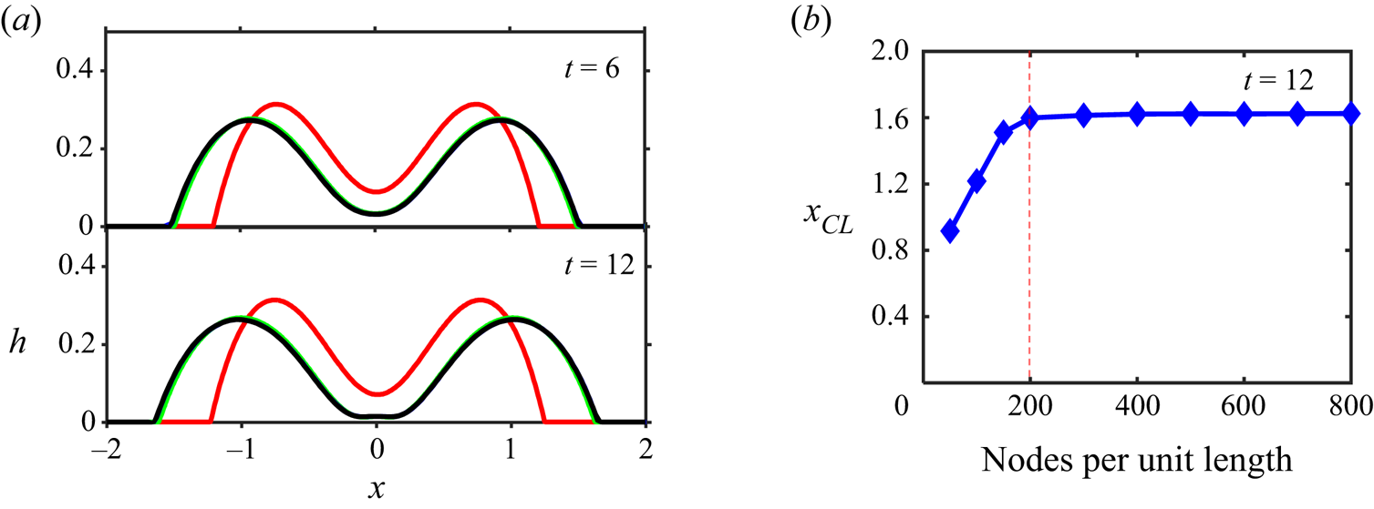
Figure 12. (a) Droplet profile for  $U_0=17\ \textrm {m}\ \textrm {s}^{-1}$, $l=7.7 \ \textrm {mm}$, $\alpha =0$, $A=0.5$ at $t=6$ and $t=12$ with different the mesh sizes: 1/100 (red), 1/200 (green), 1/400 (blue) and 1/800 (black) per length. (b) Contact-line location at $t=12$ is plotted with an increasing number of nodes per unit length.
Appendix D. Supplementary figures
The  $\alpha -U_0$ phase diagram of $l=4.9 \ \textrm {{mm}}$ for a larger range of $\alpha$ is included in figure 13. The phase diagram shows that the critical jet speed for droplet splitting increases drastically as $\alpha$ approaches 1 and basically ‘disappears’ for $\alpha >1$. This is expected because $\alpha \geqslant 1$ means that the centre of the jet no longer directly hits the droplet and is unable to split the droplet. On the other hand, the transitional velocity from hanging to depinning is shown to decrease for $\alpha < 1$ and to gradually increase for $\alpha > 1$. Since the centre of the impinging jet sits outside the droplet for $\alpha > 1$, it requires higher $U_0$ to generate sufficient asymmetry in the external pressure to depin the droplet.

Figure 13. Numerical results of the  $U_0 - \alpha$ phase diagram for $l = 4.9 \ \textrm {mm}$.
We have also reproduced figures 5, 6 and 8 by replacing  $U_0$ and $l$ with $We$ and $Bo$, respectively. The dimensionless plots are shown in figures 14, 15 and 16.
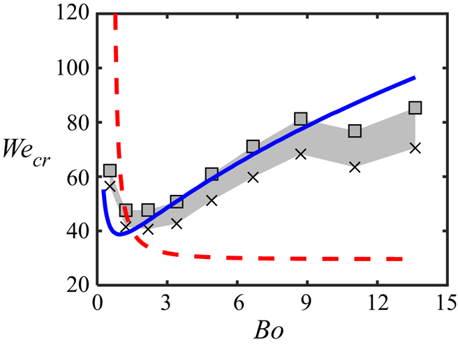
Figure 14. Plot of  $We_{cr}$ and Bo from the numerical simulations (grey area), the steady-state prediction (solid blue line) and the steady-state model with a fixed contact line by Hooshanginejad et al. (Reference Hooshanginejad, Dutcher, Shelley and Lee2020) (dashed red line).

Figure 15. The  $\alpha - We$ phase diagram for (a) $l=4.9 \ \textrm {mm}$ (or ${Bo} =1.97$) and (b) $l=7.7 \ \textrm {mm}$ (or ${Bo} =4.07$) based on the numerical simulations.
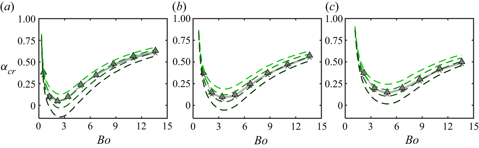
Figure 16. Simulation results and theoretical predictions of  $\alpha _{cr}$ with varying $Bo$ at $U_0=11 \ \textrm {m}\ \textrm {s}^{-1}$, whereas we set the vertical location of the nozzle to be: (a) $H=20 \ \textrm {mm}$, (b) $H=30 \ \textrm {mm}$ and (c) $H=40 \ \textrm {mm}$.


 Open access