


1. Introduction
Electrochemical processes, such as water electrolysis for hydrogen production, are a focus of efforts to develop a clean and efficient energy system. Despite progress in advancing the catalytic properties of electrode materials, the efficiency of water splitting remains affected by the gas bubbles forming and growing at the electrodes, which reduce the reaction area and impede mass transfer, causing additional energy losses (Li et al. Reference Li, Xie, Yu, Luo and Sun2023b ).
There is increased interest in structuring electrodes with regular surface elevations or alternating materials, particularly at the nano- and micrometre scales, as this may accelerate bubble detachment via reduced adhesion forces or fostered coalescence of neighbouring bubbles (Li et al. Reference Li, Xie, Yu, Luo and Sun2023b ; Bashkatov et al. Reference Bashkatov, Park, Demirkır, Wood, Koper, Lohse and Krug2024). Additionally, small catalytic islands also reduce the expenditure of noble metal catalysts. However, due to the resolution limits of optical methods, it is difficult to study the behaviour of small bubbles in experiments. Nano-bubbles are typically observed indirectly through electrical signals (Chen et al. Reference Chen, Wiedenroth, German and White2015) or light scattering (Suvira et al. Reference Suvira, Ahuja, Lovre, Singh, Draher and Zhang2023), and distinguishing them from other surface adsorbates by atomic force microscopy remains challenging.
Molecular dynamics (MD) simulations have been successfully applied to advance the understanding of electrochemical nano-bubbles (Gadea et al. Reference Gadea, Perez Sirkin, Molinero and Scherlis2020; Ma et al. Reference Ma, Guo, Chen and Zhang2021). Also, the stability theory for surface nano-bubbles developed in the last decade (Lohse & Zhang Reference Lohse and Zhang2015b ) delivered valuable insights into the bubble evolution at nano-/micro-electrodes. In particular, it was clarified that contact line pinning in an oversaturated liquid leads to the stabilisation of surface nano-bubbles in which the Laplace pressure is large (Liu & Zhang Reference Liu and Zhang2014; Lohse & Zhang Reference Lohse and Zhang2015a ). On the contrary, unpinned nano-bubbles, depending on oversaturation, will either dissolve or grow without limit but not stay stable (Lohse & Zhang Reference Lohse and Zhang2015a ). For electrochemical bubbles pinned at nano-electrodes, the influx due to electrochemically generated gas may compensate the outflux due to the Laplace pressure (Liu et al. Reference Liu, Edwards, German, Chen and White2017), and a dynamic equilibrium state is achieved. Zhang & Lohse (Reference Zhang and Lohse2023) considered a reaction-controlled growth mode for bubbles that completely cover the electrode. Here, all the gas produced at the wetted edge of the electrode directly enters the bubble, and the electrolyte remains at zero oversaturation. On the contrary, also a diffusion-controlled mode was considered, where the wetted electrode area is relatively large compared with the bubble size (Lohse & Zhang Reference Lohse and Zhang2015a ; Zhang et al. 2024). Then, diffusion of dissolved gas produced at the electrode into the bulk becomes important. Assuming a linear concentration profile, the over-saturation profile in the electrolyte can be derived from the current density. For bubbles much smaller than the thickness of the concentration boundary layer at the electrode, such as e.g. nano-bubbles, the mass transfer into the bubble can be easily calculated from the derived over-saturation (Popov Reference Popov2005). For both growth modes mentioned, a minimum current density was deduced, above which the bubble will grow without limit instead of reaching an equilibrium state.
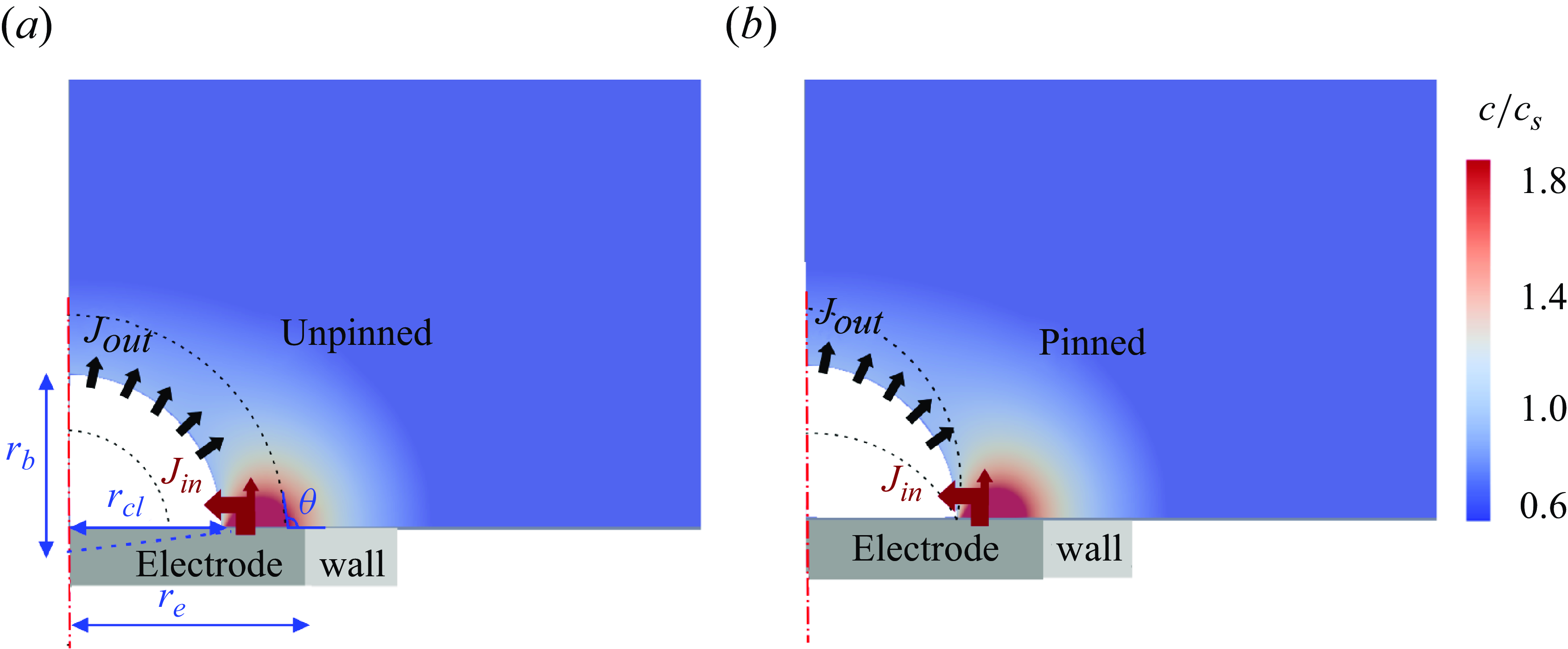
Figure 1. Sketch of the unpinned and pinned bubble evolution processes. The contour plot represents the ratio between the concentration of dissolved gas, $c$
, and the saturation concentration,
$c$
, and the saturation concentration, $c_s$
.
$c_s$
.
In addition to nano-electrodes, bubbles evolving at micro-electrodes are interesting for practical reasons and have been studied intensively in e.g. Bashkatov et al. (Reference Bashkatov, Hossain, Mutschke, Yang, Rox, Weidinger and Eckert2022) and Park et al. (Reference Park, Liu, Demirkır, van der Heijden, Lohse, Krug and Koper2023). However, the question of bubble stability still awaits a detailed investigation, which numerically is beyond the scope of MD. Unlike nano-electrodes where growing bubbles get pinned early, micro-electrodes may lead to a more complex wetting behaviour, including both pinned and unpinned manners (Yang et al. Reference Yang, Karnbach, Uhlemann, Odenbach and Eckert2015; Demirkır et al. Reference Demirkır, Wood, Lohse and Krug2024), see figure 1. The bubble growth regime can be characterised using the Damköhler number, which represents the ratio between the time scales of chemical reaction to that of advective or diffusive transport of the dissolved gas produced. In the present case, it can be reduced to $Da = A_e/r_b^2$
, which describes the ratio of the active electrode area
$Da = A_e/r_b^2$
, which describes the ratio of the active electrode area $A_e$
to the bubble surface area
$A_e$
to the bubble surface area $\sim r_b^2$
(Van Der Linde et al. Reference van der Linde, Moreno Soto, Peñas-López, Rodríguez-Rodríguez, Lohse, Gardeniers, van der Meer and Fernández Rivas2017). At micro-electrodes, depending on the value of
$\sim r_b^2$
(Van Der Linde et al. Reference van der Linde, Moreno Soto, Peñas-López, Rodríguez-Rodríguez, Lohse, Gardeniers, van der Meer and Fernández Rivas2017). At micro-electrodes, depending on the value of $Da$
, the gas produced at the electrode may not completely enter the bubble. Parts of the produced gas could diffuse into the surrounding liquid, not directly contributing to bubble growth and creating a local over-saturated region near the bubble foot. This is different from the reaction-controlled (
$Da$
, the gas produced at the electrode may not completely enter the bubble. Parts of the produced gas could diffuse into the surrounding liquid, not directly contributing to bubble growth and creating a local over-saturated region near the bubble foot. This is different from the reaction-controlled ( $Da \ll 1$
) or diffusion-controlled (
$Da \ll 1$
) or diffusion-controlled ( $Da \gg 1$
) modes considered before at the nano-scale (Zhang & Lohse Reference Zhang and Lohse2023; Zhang et al. Reference Zhang, Zhu, Wood and Lohse2024), as also the thickness of the concentration boundary layer of dissolved gas may become comparable to the radius of micrometre-sized bubbles. It prevents the application of analytical solutions for the mass transfer at the bubble surface and requires an extension of the dynamic equilibrium theory that will be presented below.
$Da \gg 1$
) modes considered before at the nano-scale (Zhang & Lohse Reference Zhang and Lohse2023; Zhang et al. Reference Zhang, Zhu, Wood and Lohse2024), as also the thickness of the concentration boundary layer of dissolved gas may become comparable to the radius of micrometre-sized bubbles. It prevents the application of analytical solutions for the mass transfer at the bubble surface and requires an extension of the dynamic equilibrium theory that will be presented below.
Once a dynamic equilibrium between the gas entering and leaving the bubble is reached, the question of the stability of the equilibrium state with respect to small disturbances of e.g. current, pressure or temperature arises. Lohse & Zhang (Reference Lohse and Zhang2015a ) already studied the stability of surface nano-bubbles in a homogeneously oversaturated liquid and found that stable equilibrium states exist for pinned bubbles, whereas unpinned bubbles are always unstable. However, when additionally an electrode reaction is taking place, a different stability behaviour of the equilibrium states may result, which has not yet been investigated.
Therefore, this work aims at studying the dynamics and stability of both pinned and unpinned hydrogen (H $_2$
) bubbles at micro-electrodes during water electrolysis, thereby accurately addressing the complex situation of the spatially inhomogeneous distribution of dissolved gas. This will be achieved by performing direct numerical simulations, based on which the existing equilibrium and stability theory will be extended by taking into account an electrode reaction that causes fluxes into both the bubble and electrolyte. Finally, this enables us to identify the parameter regions of bubble growth, dissolution and dynamic equilibrium and to demonstrate the stability of equilibrium states.
$_2$
) bubbles at micro-electrodes during water electrolysis, thereby accurately addressing the complex situation of the spatially inhomogeneous distribution of dissolved gas. This will be achieved by performing direct numerical simulations, based on which the existing equilibrium and stability theory will be extended by taking into account an electrode reaction that causes fluxes into both the bubble and electrolyte. Finally, this enables us to identify the parameter regions of bubble growth, dissolution and dynamic equilibrium and to demonstrate the stability of equilibrium states.
2. Numerical modelling
The gas-liquid interface is resolved using a geometric volume-of-fluid method in Basilisk (Popinet Reference Popinet2013). For an incompressible two-phase flow with phase change, the transport equation of the volume fraction of the liquid phase, $\alpha _l$
, can be derived from mass conservation
$\alpha _l$
, can be derived from mass conservation
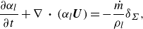 \begin{equation} \frac {\partial \alpha _l}{\partial t} + \nabla \,\boldsymbol\cdot\, (\alpha _l \boldsymbol{U}) = - \frac {\dot {m}}{ \rho _l} \delta _{\scriptstyle \Sigma }, \end{equation}
with $\alpha _l=1$
and 0 indicating the liquid (
$\alpha _l=1$
and 0 indicating the liquid ( $l$
) and gas (
$l$
) and gas ( $g$
) phases, respectively. The density
$g$
) phases, respectively. The density $\rho$
and the viscosity
$\rho$
and the viscosity $\mu$
can be calculated based on the arithmetic mean of the volume fractions of the phases
$\mu$
can be calculated based on the arithmetic mean of the volume fractions of the phases
 \begin{equation} \rho = \alpha _l \rho _l + (1-\alpha _l) \rho _g, \ \ \ \ \ \mu = \alpha _l \mu _l + (1-\alpha _l) \mu _g. \end{equation}
The right-hand-side of (2.1) represents the source term due to phase change, with $ \delta _{\scriptstyle \Sigma }$
denoting the surface Dirac function that has a non-zero value only at the interface
$ \delta _{\scriptstyle \Sigma }$
denoting the surface Dirac function that has a non-zero value only at the interface $\Sigma$
. The mass transfer rate per unit interface surface area,
$\Sigma$
. The mass transfer rate per unit interface surface area, $\dot {m}$
, is calculated according to Fick’s law and will be introduced later. In a one-fluid framework, as presented here,
$\dot {m}$
, is calculated according to Fick’s law and will be introduced later. In a one-fluid framework, as presented here, $\boldsymbol{U}$
is the mixture velocity of both phases, that needs to fulfil the Navier–Stokes equation complemented with the continuity equation
$\boldsymbol{U}$
is the mixture velocity of both phases, that needs to fulfil the Navier–Stokes equation complemented with the continuity equation
 \begin{align} \frac {\partial (\rho \boldsymbol{U} )}{\partial t}+ \nabla \,\boldsymbol\cdot\, ( \rho \boldsymbol{U} \boldsymbol{U}) & = - \nabla p + \nabla \,\boldsymbol\cdot\, \lbrace \mu (\nabla {\boldsymbol{U} + (\nabla U)^T}) \rbrace +\boldsymbol{f_\gamma },\end{align}
 \begin{align} \nabla \,\boldsymbol\cdot\, {\boldsymbol{U}} & =\dot {m} \left ( \frac {1}{\rho _g} - \frac {1}{\rho _l} \right) \delta _{\scriptstyle \Sigma }.\end{align}
Here, $p$
is the pressure and
$p$
is the pressure and $\boldsymbol{f_\gamma } = \gamma \kappa \boldsymbol{n_{\scriptstyle \Sigma }} \delta _{\scriptstyle \Sigma }$
is the surface tension force, with
$\boldsymbol{f_\gamma } = \gamma \kappa \boldsymbol{n_{\scriptstyle \Sigma }} \delta _{\scriptstyle \Sigma }$
is the surface tension force, with $\gamma, \, \kappa, \, \boldsymbol{n_{\scriptstyle \Sigma }}$
denoting the surface tension, the interface curvature and the normal unit vector, respectively. To accurately calculate
$\gamma, \, \kappa, \, \boldsymbol{n_{\scriptstyle \Sigma }}$
denoting the surface tension, the interface curvature and the normal unit vector, respectively. To accurately calculate $\boldsymbol{f_\gamma }$
, a height function method combined with a balanced-force discretisation scheme (Popinet Reference Popinet2009) is used. The contact angle at the electrode surface is specified by the height function in the surface mesh cells (Afkhami & Bussmann Reference Afkhami and Bussmann2008).
$\boldsymbol{f_\gamma }$
, a height function method combined with a balanced-force discretisation scheme (Popinet Reference Popinet2009) is used. The contact angle at the electrode surface is specified by the height function in the surface mesh cells (Afkhami & Bussmann Reference Afkhami and Bussmann2008).
The species transport equation of the dissolved gas ( $c$
) in the liquid is solved with a source term to account for the mass transfer at the interface
$c$
) in the liquid is solved with a source term to account for the mass transfer at the interface
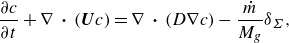 \begin{equation} \frac {\partial c}{\partial t} + \nabla \,\boldsymbol\cdot\, (\boldsymbol{U} c) = \nabla \,\boldsymbol\cdot\, (D \nabla c) -\frac {\dot {m}}{ M_{{g}}} \delta _{\scriptstyle \Sigma }, \end{equation}
with $D$
and
$D$
and $M_g$
representing the diffusion coefficient and the molar mass of the dissolved gas. Based on the spatial distribution of
$M_g$
representing the diffusion coefficient and the molar mass of the dissolved gas. Based on the spatial distribution of $c$
, the diffusional mass transfer rate
$c$
, the diffusional mass transfer rate $\dot {m}$
can be computed using Fick’s law
$\dot {m}$
can be computed using Fick’s law
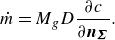 \begin{equation} \dot {m}= M_{{g}} D \dfrac {\partial c}{\partial \boldsymbol{n_{\scriptstyle \Sigma }}}. \end{equation}
The simulation parameter ranges are selected so as to match with typical micro-electrode experiments (Van Der Linde et al. Reference van der Linde, Moreno Soto, Peñas-López, Rodríguez-Rodríguez, Lohse, Gardeniers, van der Meer and Fernández Rivas2017; Bashkatov et al. Reference Bashkatov, Hossain, Mutschke, Yang, Rox, Weidinger and Eckert2022). The electrode radius $r_e$
ranges from 5.5 to 100
$r_e$
ranges from 5.5 to 100 $\unicode {x03BC}$
m, which might be of practical relevance also for catalytic islands on larger electrodes in industrial electrolysis. An axisymmetric computational domain with a side length of 10
$\unicode {x03BC}$
m, which might be of practical relevance also for catalytic islands on larger electrodes in industrial electrolysis. An axisymmetric computational domain with a side length of 10 $r_{b,\textit{ini}}$
is used, with initial bubble radii of
$r_{b,\textit{ini}}$
is used, with initial bubble radii of $r_{b,\textit{ini}} = 5 - 50$ $\unicode {x03BC}$
m. Different constant current densities of
$\unicode {x03BC}$
m. Different constant current densities of $j=2.5-1250$
A m
$j=2.5-1250$
A m ${^-}^2$
are applied to the wetted part of the electrode surface to resemble a potentiostatic operation mode, where a constant potential difference is applied between the reference and the working electrode. Here, the cell current will reduce if a growing bubble blocks larger parts of the electrode. According to Faraday’s law, it yields corresponding Neumann boundary conditions of the concentration
${^-}^2$
are applied to the wetted part of the electrode surface to resemble a potentiostatic operation mode, where a constant potential difference is applied between the reference and the working electrode. Here, the cell current will reduce if a growing bubble blocks larger parts of the electrode. According to Faraday’s law, it yields corresponding Neumann boundary conditions of the concentration $c$
of dissolved H
$c$
of dissolved H $_2$
at the wetted electrode part, i.e.
$_2$
at the wetted electrode part, i.e. $\partial c/\partial n = j/(zFD)$
, with
$\partial c/\partial n = j/(zFD)$
, with $z=2$
and
$z=2$
and $F=96\,485$
representing the charge number of the hydrogen evolution reaction and the Faraday constant, respectively. At the remaining bottom wall, see figure 1, a no-flux condition (
$F=96\,485$
representing the charge number of the hydrogen evolution reaction and the Faraday constant, respectively. At the remaining bottom wall, see figure 1, a no-flux condition ( $\partial c/\partial n=0$
) is applied to the dissolved gas concentration. For unpinned bubbles, static water-side contact angles
$\partial c/\partial n=0$
) is applied to the dissolved gas concentration. For unpinned bubbles, static water-side contact angles $\theta$
ranging from 45° to 90°, as shown in figure 1, are imposed. As we focus on the initial growth and stability of bubbles, the rapid change of
$\theta$
ranging from 45° to 90°, as shown in figure 1, are imposed. As we focus on the initial growth and stability of bubbles, the rapid change of $\theta$
shortly before detachment is not considered. For the pinning cases considered, the bubble coverage on the electrode varies between 45 % and 90 %. To keep the bubble pinned, we apply sufficiently large (150°) and small (30°) contact angles inside and outside the pinning point, respectively (Sakakeeny et al. Reference Sakakeeny, Deshpande, Deb, Alvarado and Ling2021). Considering the slow or no motion of the contact line, a no-slip condition is used at the bottom boundary, which is validated in figure 12 in Appendix B. Initially, we set the flow velocity to zero and the concentration to the bulk value
$\theta$
shortly before detachment is not considered. For the pinning cases considered, the bubble coverage on the electrode varies between 45 % and 90 %. To keep the bubble pinned, we apply sufficiently large (150°) and small (30°) contact angles inside and outside the pinning point, respectively (Sakakeeny et al. Reference Sakakeeny, Deshpande, Deb, Alvarado and Ling2021). Considering the slow or no motion of the contact line, a no-slip condition is used at the bottom boundary, which is validated in figure 12 in Appendix B. Initially, we set the flow velocity to zero and the concentration to the bulk value $c_{b}$
. As often the initial hydrogen concentration in the bulk can be neglected compared with that at the bubble interface (Van Der Linde et al. Reference van der Linde, Moreno Soto, Peñas-López, Rodríguez-Rodríguez, Lohse, Gardeniers, van der Meer and Fernández Rivas2017; Gadea et al. Reference Gadea, Perez Sirkin, Molinero and Scherlis2020), we consider under-saturated/saturated electrolytes. With
$c_{b}$
. As often the initial hydrogen concentration in the bulk can be neglected compared with that at the bubble interface (Van Der Linde et al. Reference van der Linde, Moreno Soto, Peñas-López, Rodríguez-Rodríguez, Lohse, Gardeniers, van der Meer and Fernández Rivas2017; Gadea et al. Reference Gadea, Perez Sirkin, Molinero and Scherlis2020), we consider under-saturated/saturated electrolytes. With $c_s$
denoting the saturation concentration at given external pressure, the over-saturation follows
$c_s$
denoting the saturation concentration at given external pressure, the over-saturation follows $\zeta =c_{b}/c_{s}-1 \leqslant 0$
. If not stated otherwise, we consider
$\zeta =c_{b}/c_{s}-1 \leqslant 0$
. If not stated otherwise, we consider $c_b=0$
, and thus
$c_b=0$
, and thus $\zeta =-1$
.
$\zeta =-1$
.
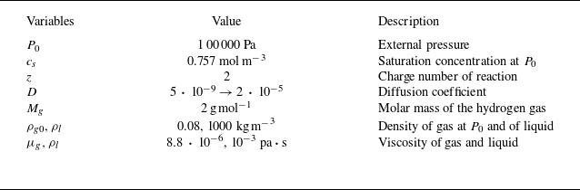
The material parameters used in the simulations, see table 1, apply to water electrolysis in an aqueous electrolyte at standard conditions, except that the diffusion coefficient is manually increased to accelerate the simulations. By rescaling the time according to the ratio of the increased to the real diffusion coefficient, the original bubble evolution can be recovered for the conditions considered in this work (Han et al. Reference Han, Haung, Eckert and Mutschke2025), see also figure 12 in the Appendix.
Table 1. Material properties used in the simulations.
To further ensure accuracy of the simulations, an adaptive mesh refinement technique available in Basilisk is applied, as a result of which the initial mesh size of $\sim$
0.3
$\sim$
0.3 $r_{b,\textit{ini}}$
near the gas-liquid interface gets refined down to
$r_{b,\textit{ini}}$
near the gas-liquid interface gets refined down to $\sim$
0.01
$\sim$
0.01 $r_{b,\textit{ini}}$
during the simulations. The tolerance of the iterative solver is set to be
$r_{b,\textit{ini}}$
during the simulations. The tolerance of the iterative solver is set to be $10^{-6}$
, and the time step is automatically adjusted to keep the Courant-Friedrichs-Lewy (CFL) number below 0.5 during the simulations. Finally, the presented numerical model (equations (2.1)
$10^{-6}$
, and the time step is automatically adjusted to keep the Courant-Friedrichs-Lewy (CFL) number below 0.5 during the simulations. Finally, the presented numerical model (equations (2.1) $-$
(2.6)) implemented in Basilisk has already been successfully validated against the analytical solutions of Epstein–Plesset and Scriven for the dissolution and growth of bulk bubbles in under- and over-saturated liquids (Gennari et al. Reference Gennari, Jefferson-Loveday and Pickering2022).
$-$
(2.6)) implemented in Basilisk has already been successfully validated against the analytical solutions of Epstein–Plesset and Scriven for the dissolution and growth of bulk bubbles in under- and over-saturated liquids (Gennari et al. Reference Gennari, Jefferson-Loveday and Pickering2022).
3. Results and discussion
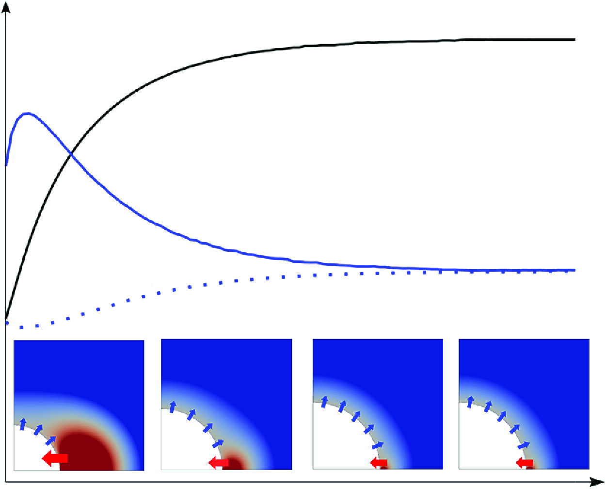
Figure 2 shows simulation results of how an unpinned and a pinned bubble develop over time, and quantifies the mass transfer across the bubble surface. Due to the electrode reaction, a high-concentration region of dissolved H $_2$
near the wetted electrode part (red-colour region) is clearly visible. The growth of the unpinned bubble (top) increases the electrode blockage. This reduces the amount of gas diffusing into the liquid, and the high-concentration region decreases in size. As shown in figure 1, this reduces the gas influx
$_2$
near the wetted electrode part (red-colour region) is clearly visible. The growth of the unpinned bubble (top) increases the electrode blockage. This reduces the amount of gas diffusing into the liquid, and the high-concentration region decreases in size. As shown in figure 1, this reduces the gas influx $ J_{in}$
, defined as the mole amount of gas per second, into the bubble across the interface near the bottom, where the liquid is over-saturated. In contrast, the magnitude of the gas outflux
$ J_{in}$
, defined as the mole amount of gas per second, into the bubble across the interface near the bottom, where the liquid is over-saturated. In contrast, the magnitude of the gas outflux $\left | J_{out} \right |$
([mol s−1]) across the bubble interface into the under-saturated bulk liquid increases with the expanding bubble surface area. Note that values of
$\left | J_{out} \right |$
([mol s−1]) across the bubble interface into the under-saturated bulk liquid increases with the expanding bubble surface area. Note that values of $J_{out}$
are negative, as defined later in equation (3.2). As shown in the upper part of sub-figure 2(b), both fluxes counterbalance at approximately 30 s, at which the bubble reaches a dynamic equilibrium state, visible by the levelling off of its radius. For the case of a pinned contact line (bottom), the contact angle reduces with time until an equilibrium is reached after 80s. Although the wetted electrode area remains constant, the high-
$J_{out}$
are negative, as defined later in equation (3.2). As shown in the upper part of sub-figure 2(b), both fluxes counterbalance at approximately 30 s, at which the bubble reaches a dynamic equilibrium state, visible by the levelling off of its radius. For the case of a pinned contact line (bottom), the contact angle reduces with time until an equilibrium is reached after 80s. Although the wetted electrode area remains constant, the high- $c_{{H_2}}$
region seems to slightly diminish, as the smaller contact angle also reduces gas transport into the bulk. The lower part of sub-figure 2(b) shows numerical results of the temporal behaviour of
$c_{{H_2}}$
region seems to slightly diminish, as the smaller contact angle also reduces gas transport into the bulk. The lower part of sub-figure 2(b) shows numerical results of the temporal behaviour of $J_{in}$
and
$J_{in}$
and $J_{out}$
. The influx caused by the oversaturation near the bubble foot is computed based on Faraday’s law (see (3.1) below), and the outflux is computed as the sum of the local molar gas transfer rates along the interface. As can be seen, the evolution of the bubble leads to an increase in
$J_{out}$
. The influx caused by the oversaturation near the bubble foot is computed based on Faraday’s law (see (3.1) below), and the outflux is computed as the sum of the local molar gas transfer rates along the interface. As can be seen, the evolution of the bubble leads to an increase in $ J_{in}$
with time, while
$ J_{in}$
with time, while $\left | J_{out} \right |$
also rises with the growing bubble surface area, until both converge. Therefore, a dynamic equilibrium is found for both unpinned and pinned bubbles at micro-electrodes, which will be further analysed below.
$\left | J_{out} \right |$
also rises with the growing bubble surface area, until both converge. Therefore, a dynamic equilibrium is found for both unpinned and pinned bubbles at micro-electrodes, which will be further analysed below.

Figure 2. (a) Numerical results of the evolution of an unpinned (top) and a pinned (bottom) bubble. The coloured surface represents the distribution of dissolved gas concentration normalised by the saturation concentration $c_s$
, the green bottom line marks the electrode. (b) Evolution of
$c_s$
, the green bottom line marks the electrode. (b) Evolution of $r_b$
and
$r_b$
and $\theta$
with time. The time instants shown left are marked by red dots in the right graphs. For the unpinned case:
$\theta$
with time. The time instants shown left are marked by red dots in the right graphs. For the unpinned case: $r_e=100\, \unicode {x03BC}$
m,
$r_e=100\, \unicode {x03BC}$
m, $j=125$
A m
$j=125$
A m ${^-}^2$
,
${^-}^2$
, $\theta = 90$
°,
$\theta = 90$
°, $r_{b,\textit{ini}}=50\, \unicode {x03BC}$
m. For the pinned case:
$r_{b,\textit{ini}}=50\, \unicode {x03BC}$
m. For the pinned case: $r_e=55\, \unicode {x03BC}$
m,
$r_e=55\, \unicode {x03BC}$
m, $j=250$
A m
$j=250$
A m ${^-}^2$
,
${^-}^2$
, $r_{\textit{cl}}=50 \, \unicode {x03BC}$
m,
$r_{\textit{cl}}=50 \, \unicode {x03BC}$
m, $\theta _{{\textit{ini}}}=90$
°.
$\theta _{{\textit{ini}}}=90$
°.
3.1. Theoretical analysis
As can be seen from figure 2, in both cases of pinned and unpinned growth, the bubbles at equilibrium cover most parts of the electrode. Despite this corresponding to small values of the Damköhler number (see also Appendix E), diffusion into the surrounding electrolyte still takes place, as evidenced by the red high-concentration regions near the bubble foot. This motivates us to start from the reaction-controlled modelling (Zhang & Lohse Reference Zhang and Lohse2023), which calculates the gas entering the bubble directly from the current density $j$
, but to additionally introduce a correction factor
$j$
, but to additionally introduce a correction factor $0\lt f_{in} \leqslant 1$
accounting for gas remaining in the electrolyte, so that only a part of the gas produced at the electrode enters the bubble. The gas influx
$0\lt f_{in} \leqslant 1$
accounting for gas remaining in the electrolyte, so that only a part of the gas produced at the electrode enters the bubble. The gas influx $J_{in}$
across the bubble surface can then be described as follows:
$J_{in}$
across the bubble surface can then be described as follows:
 \begin{equation} J_{in} = f_{in} \,\boldsymbol\cdot\, J_{e} = f_{in} \,\boldsymbol\cdot\, \dfrac { j \pi (r_e^2 - r_{\textit{cl}}^2)}{ z F}, \end{equation}
with $J_e, \, r_e, \, r_{\textit{cl}}, \, z, \, F$
denoting the gas flux generated at the electrode, the radius of the electrode and the bubble contact line, the charge number and the Faraday constant. Unlike Zhang & Lohse (Reference Zhang and Lohse2023), in which the bubble is pinned at the edge of the nano-electrode and the gas influx is given as a constant value, here the gas influx dynamically depends on the motion of the bubble contact line and the resulting wetted electrode surface area. Values of
$J_e, \, r_e, \, r_{\textit{cl}}, \, z, \, F$
denoting the gas flux generated at the electrode, the radius of the electrode and the bubble contact line, the charge number and the Faraday constant. Unlike Zhang & Lohse (Reference Zhang and Lohse2023), in which the bubble is pinned at the edge of the nano-electrode and the gas influx is given as a constant value, here the gas influx dynamically depends on the motion of the bubble contact line and the resulting wetted electrode surface area. Values of $f_{in}$
are derived from numerical simulations for different reaction conditions by computing the ratio of the gas flux that actually enters the bubble and that produced at the electrode. As shown in figure 3,
$f_{in}$
are derived from numerical simulations for different reaction conditions by computing the ratio of the gas flux that actually enters the bubble and that produced at the electrode. As shown in figure 3, $f_{in}$
increases towards 1 with enhancing
$f_{in}$
increases towards 1 with enhancing $j$
, where the bubbles grow larger and the gas loss into the bulk reduces. At more hydrophilic surfaces, the bubble shape will increasingly impede gas transport towards the bulk, figure 2, thus causing also a higher
$j$
, where the bubbles grow larger and the gas loss into the bulk reduces. At more hydrophilic surfaces, the bubble shape will increasingly impede gas transport towards the bulk, figure 2, thus causing also a higher $f_{in}$
.
$f_{in}$
.
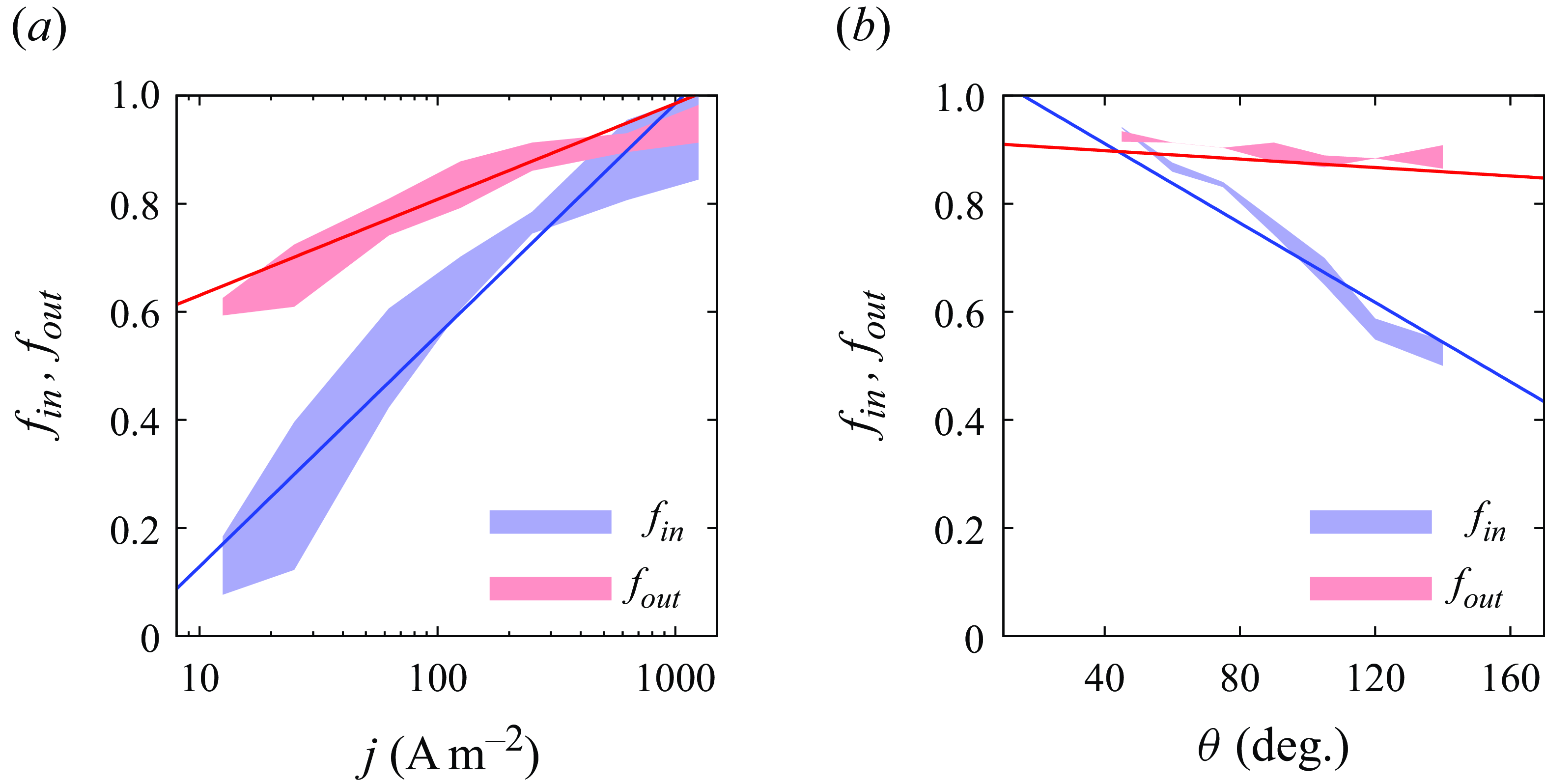
Figure 3. Values of $f_{in}$
and
$f_{in}$
and $f_{out}$
derived from numerical data when unpinned bubbles reach an equilibrium in a liquid of
$f_{out}$
derived from numerical data when unpinned bubbles reach an equilibrium in a liquid of $\zeta = -1$
, i.e.
$\zeta = -1$
, i.e. $c_b=0$
. (a) Influence of the applied current density. Here,
$c_b=0$
. (a) Influence of the applied current density. Here, $r_{b,{\textit{ini}}}=50 \, \unicode {x03BC}$
m,
$r_{b,{\textit{ini}}}=50 \, \unicode {x03BC}$
m, $\theta =90$
°, colour region represents data range obtained by
$\theta =90$
°, colour region represents data range obtained by $r_e=50-150\, \unicode {x03BC}$
m. (b) Influence of the contact angle. Here,
$r_e=50-150\, \unicode {x03BC}$
m. (b) Influence of the contact angle. Here, $j=250$
A m
$j=250$
A m ${^-}^2$
, colour region represents data range obtained by
${^-}^2$
, colour region represents data range obtained by $r_{b,{\textit{ini}}}=50 \, \unicode {x03BC}$
m,
$r_{b,{\textit{ini}}}=50 \, \unicode {x03BC}$
m, $r_e = 150\, \unicode {x03BC}$
m or
$r_e = 150\, \unicode {x03BC}$
m or $r_{b,{\textit{ini}}}=100\, \unicode {x03BC}$
m,
$r_{b,{\textit{ini}}}=100\, \unicode {x03BC}$
m, $r_e = 125\, \unicode {x03BC}$
m. Solid lines represent fitting functions ((A1), (A2) in Appendix A) used in the theoretical solutions.
$r_e = 125\, \unicode {x03BC}$
m. Solid lines represent fitting functions ((A1), (A2) in Appendix A) used in the theoretical solutions.
When the surrounding liquid is under-/saturated ( $\zeta \leqslant 0$
), at the same time, gas may diffuse out of the bubble. For the cases considered in this work, the Péclet number
$\zeta \leqslant 0$
), at the same time, gas may diffuse out of the bubble. For the cases considered in this work, the Péclet number $Pe = r_b /D \,\boldsymbol\cdot\, {\rm d}r_b/{\rm d}t \ll 1$
, indicating that convective effects are negligibly small compared with diffusion. When further neglecting initial transients, the gas transport equation,(2.5), can be simplified for steady states to
$Pe = r_b /D \,\boldsymbol\cdot\, {\rm d}r_b/{\rm d}t \ll 1$
, indicating that convective effects are negligibly small compared with diffusion. When further neglecting initial transients, the gas transport equation,(2.5), can be simplified for steady states to $\nabla ^2 c = 0$
. Combining this with Fick and Henry’s law (Popov Reference Popov2005; Lohse & Zhang Reference Lohse and Zhang2015a
), the gas outflux
$\nabla ^2 c = 0$
. Combining this with Fick and Henry’s law (Popov Reference Popov2005; Lohse & Zhang Reference Lohse and Zhang2015a
), the gas outflux $J_{out}$
reads
$J_{out}$
reads
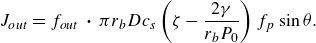 \begin{equation} J_{out} = f_{out} \,\boldsymbol\cdot\, \pi r_b D c_{s}\left ( \zeta - \dfrac {2 \gamma }{r_b P_0} \right ) f_p \sin \theta . \end{equation}
Here, $r_b, \, D, \, \gamma$
denote the bubble radius, the gas diffusion coefficient and the surface tension. The shape factor
$r_b, \, D, \, \gamma$
denote the bubble radius, the gas diffusion coefficient and the surface tension. The shape factor $f_p$
introduced by Popov (Reference Popov2005), see Appendix (A1), depends only on the water-side contact angle
$f_p$
introduced by Popov (Reference Popov2005), see Appendix (A1), depends only on the water-side contact angle $\theta$
, and monotonically decreases from infinity towards unity when
$\theta$
, and monotonically decreases from infinity towards unity when $\theta$
increases from 0° to 180°. In addition to previous work, now the factor
$\theta$
increases from 0° to 180°. In addition to previous work, now the factor $0\lt f_{out}\leqslant 1$
is introduced in (3.2). It accounts for reduced outflux due to a high-concentration region appearing near the bubble foot due to the electrode reaction (figure 2). In more detail, it is defined as the fraction of the bubble surface area where gas leaves the bubble. For
$0\lt f_{out}\leqslant 1$
is introduced in (3.2). It accounts for reduced outflux due to a high-concentration region appearing near the bubble foot due to the electrode reaction (figure 2). In more detail, it is defined as the fraction of the bubble surface area where gas leaves the bubble. For $f_{out}=1$
, equation (3.2) simplifies to the purely reaction-controlled case treated earlier (Zhang & Lohse Reference Zhang and Lohse2023), where all dissolved gas produced at the electrode immediately enters the bubble, and no region of enhanced concentration near the bubble foot is arising. The behaviour of
$f_{out}=1$
, equation (3.2) simplifies to the purely reaction-controlled case treated earlier (Zhang & Lohse Reference Zhang and Lohse2023), where all dissolved gas produced at the electrode immediately enters the bubble, and no region of enhanced concentration near the bubble foot is arising. The behaviour of $f_{out}$
determined from numerical simulations is shown in figure 3, where the coloured regions mark the results obtained for various configurations given in the caption. Similarly to
$f_{out}$
determined from numerical simulations is shown in figure 3, where the coloured regions mark the results obtained for various configurations given in the caption. Similarly to $f_{in}$
,
$f_{in}$
, $f_{out}$
increases with
$f_{out}$
increases with $j$
as the bubbles become larger. The contact angle seems to have only a minor influence. Note that, for the different configurations, only small variations in
$j$
as the bubbles become larger. The contact angle seems to have only a minor influence. Note that, for the different configurations, only small variations in $f_{in}$
and
$f_{in}$
and $f_{out}$
are observed, which motivates us to approximate both by fitting functions (solid lines), as detailed in Appendix (A1).
$f_{out}$
are observed, which motivates us to approximate both by fitting functions (solid lines), as detailed in Appendix (A1).
Mass transfer at the gas–liquid interface determines how the bubble geometry evolves with time. The change rate of the bubble mass can be expressed as
 \begin{equation} \dfrac {{\rm d}m}{{\rm d}t} = M_g\left (J_{in} + J_{out}\right ), \end{equation}
with $M_g$
denoting the molar mass of the gas. For bubbles of nano- and micrometre size, we take into account also the possible change of the gas density
$M_g$
denoting the molar mass of the gas. For bubbles of nano- and micrometre size, we take into account also the possible change of the gas density $\rho _g$
with pressure
$\rho _g$
with pressure
 \begin{equation} \dfrac {{\rm d}m}{{\rm d}t} = \dfrac {{\rm d} (\rho _g V)}{{\rm d}t} = \rho _g \dfrac {{\rm d}V}{{\rm d}t} + V \dfrac {{\rm d} \rho _g}{{\rm d}t}, \end{equation}
with
 \begin{equation} \rho _g =\rho _{g0}\left (1 + \dfrac {2 \gamma }{r_b P_0}\right ) \dfrac { (P_0 b + k_B T)}{P_0 b \left (1 + \dfrac {2 \gamma }{r_b P_0}\right ) + k_B T}, \end{equation}
where $\rho _{g0}, \, b, \, k_B, \, T$
represent the gas density at pressure
$\rho _{g0}, \, b, \, k_B, \, T$
represent the gas density at pressure $P_0$
, the volume per atom with an effective atomic radius of 0.2 nm, the Boltzmann constant and the temperature, respectively (Zhang & Lohse Reference Zhang and Lohse2023).
$P_0$
, the volume per atom with an effective atomic radius of 0.2 nm, the Boltzmann constant and the temperature, respectively (Zhang & Lohse Reference Zhang and Lohse2023).
Depending on the reaction parameters, the bubble could grow ( $ J_{in}+ J_{out}\gt 0$
) or shrink (
$ J_{in}+ J_{out}\gt 0$
) or shrink ( $J_{in}+ J_{out} \lt 0$
) with time. When assuming bubble caps of spherical shape, the relation between volume, contact angle and radius is
$J_{in}+ J_{out} \lt 0$
) with time. When assuming bubble caps of spherical shape, the relation between volume, contact angle and radius is
 \begin{equation} V =\dfrac { \pi r_{{b}}^3 ( 2 + 3 \cos \theta - \cos ^3\theta )}{3}, \, \, \, \, r_{\textit{cl}} = r_b \sin {\theta }. \end{equation}
Now, combining equations (3.3)–(3.5), a relation for the evolution of an unpinned bubble with constant contact angle can be derived
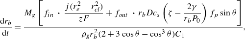 \begin{equation} \frac {{\rm d} r_b}{{\rm d}t} = \dfrac {M_g \left [ f_{in} \,\boldsymbol\cdot\, \dfrac { j (r_e^2 - r_{\textit{cl}}^2)}{ z F} + f_{out} \,\boldsymbol\cdot\, r_b D c_{s}\left ( \zeta - \dfrac {2 \gamma }{r_b P_0} \right ) f_p \sin \theta \right ]}{ \rho _g r_b^2 ( 2 + 3 \cos \theta - \cos ^3\theta ) C_1 }, \end{equation}
with $C_1$
describing the influence of a variable gas density
$C_1$
describing the influence of a variable gas density
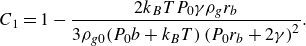 \begin{equation} C_1 = 1 - \dfrac {2k_B T P_0 \gamma \rho _g r_b}{3 \rho _{g0} (P_0 b + k_B T)\left (P_0r_b + 2\gamma \right )^2}. \end{equation}
For the case of a pinned bubble, the temporal change of the contact angle is derived similarly as
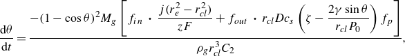 \begin{equation} \frac {{\rm d} \theta }{{\rm d}t} = \dfrac {- (1-\cos {\theta })^2M_g\left [ f_{in} \,\boldsymbol\cdot\, \dfrac { j (r_e^2 - r_{\textit{cl}}^2)}{ z F} + f_{out} \,\boldsymbol\cdot\, r_{\textit{cl}} D c_{s}\left ( \zeta - \dfrac {2 \gamma \sin {\theta }}{r_{\textit{cl}} P_0} \right ) f_p \right ]}{ \rho _g r_{\textit{cl}}^3 C_2}, \end{equation}
with $C_2$
given as
$C_2$
given as
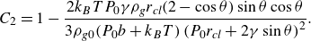 \begin{equation} C_2 = 1 - \dfrac {2 k_B T P_0 \gamma \rho _g r_{\textit{cl}}(2-\cos \theta )\sin \theta \cos {\theta }}{ 3 \rho _{g0} (P_0 b + k_B T)\left (P_0 r_{\textit{cl}} +2 \gamma \sin \theta \right )^2 }. \end{equation}
We remark that our expression (3.9) is equivalent to (3.5) in Zhang & Lohse (Reference Zhang and Lohse2023) if $f_{in}=f_{out}=1$
. Under the conditions considered in this study, the varying gas density is found to influence the initial dynamics of bubbles smaller than 5
$f_{in}=f_{out}=1$
. Under the conditions considered in this study, the varying gas density is found to influence the initial dynamics of bubbles smaller than 5 $\unicode {x03BC}$
m, corresponding to a relative density change
$\unicode {x03BC}$
m, corresponding to a relative density change $\Delta \rho _g/\rho _{g0}$
larger than
$\Delta \rho _g/\rho _{g0}$
larger than $\sim$
29 %, or
$\sim$
29 %, or $C_1,\, C_2$
smaller than
$C_1,\, C_2$
smaller than $\sim$
0.9. For sufficiently large bubbles,
$\sim$
0.9. For sufficiently large bubbles, $\rho _g$
approaches
$\rho _g$
approaches $\rho _{g0}$
, and
$\rho _{g0}$
, and $C_1,\, C_2$
approach 1, which allows us to simplify equations (3.7), (3.9) for a constant gas density. For more details we refer the reader to Appendix (A2).
$C_1,\, C_2$
approach 1, which allows us to simplify equations (3.7), (3.9) for a constant gas density. For more details we refer the reader to Appendix (A2).
If during the evolution of the bubble, a counterbalance between $J_{in}$
and
$J_{in}$
and $J_{out}$
is reached, as shown in figure 2, a dynamic equilibrium is found. From (3.1), 3.2, it can be derived that
$J_{out}$
is reached, as shown in figure 2, a dynamic equilibrium is found. From (3.1), 3.2, it can be derived that
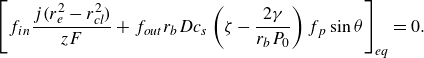 \begin{equation} \left [ f_{in} \dfrac { j (r_e^2 - r_{\textit{cl}}^2)}{ z F} + f_{out} r_{b} D c_{s}\left ( \zeta - \dfrac {2 \gamma }{r_{b} P_0} \right ) f_p \sin \theta \right ]_{eq} = 0. \end{equation}
Subscript eq denotes equilibrium. Equation (3.11) allows us to determine $r_{b,eq}$
or
$r_{b,eq}$
or $\theta _{eq}$
for unpinned or pinned bubbles, respectively. If no root can be found for the given conditions, an equilibrium will not occur, and the bubble either grows without limit or completely dissolves.
$\theta _{eq}$
for unpinned or pinned bubbles, respectively. If no root can be found for the given conditions, an equilibrium will not occur, and the bubble either grows without limit or completely dissolves.
Once a dynamic equilibrium is reached, minor fluctuations in the system parameters such as current, pressure or temperature may disturb the balance between the in- and out-fluxes, causing the bubble to start growing, dissolving or reshaping. In the case of a stable equilibrium, the resulting modified fluxes will bring the bubble back to the equilibrium state. For example, if an unpinned bubble becomes temporarily larger than $r_{b,eq}$
,
$r_{b,eq}$
, $J_{in}$
will decrease due to the reduced wetted electrode area, whereas the bubble surface area and therefore
$J_{in}$
will decrease due to the reduced wetted electrode area, whereas the bubble surface area and therefore $\left | J_{out} \right |$
increase. Thus, both changes tend to bring the bubble back to
$\left | J_{out} \right |$
increase. Thus, both changes tend to bring the bubble back to $r_{b,eq}$
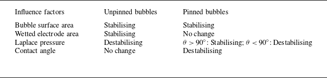
. Other factors influencing the stability are analysed in table 2. As it is difficult to decide which is the determining factor, we apply the methodology of Lohse & Zhang (Reference Lohse and Zhang2015a
) for studying the stability of surface nano-bubbles and extend it by additionally taking into account the gas production at the electrode. The stability of unpinned and pinned bubbles requires
$r_{b,eq}$
. Other factors influencing the stability are analysed in table 2. As it is difficult to decide which is the determining factor, we apply the methodology of Lohse & Zhang (Reference Lohse and Zhang2015a
) for studying the stability of surface nano-bubbles and extend it by additionally taking into account the gas production at the electrode. The stability of unpinned and pinned bubbles requires
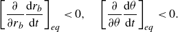 \begin{equation} \left [\dfrac { \partial }{\partial r_b}\frac {{\rm d}r_b}{{\rm d}t}\right ]_{eq} \lt 0, \, \, \, \, \, \left [\dfrac { \partial }{\partial \theta } \frac {{\rm d}\theta }{{\rm d}t}\right ]_{eq} \lt 0. \end{equation}
For unpinned surface bubbles, combining (3.7) and (3.11), we obtain (derivation in Appendix (A3))
 \begin{equation} \left [ \dfrac { \partial }{\partial r_b} \frac {{\rm d}r_b}{{\rm d}t} \right ]_{eq} =\dfrac {M_g }{\rho _g ( 2 + 3 \cos \theta - \cos ^3\theta ) r_{b,eq}^2 C_{1,eq}} \left [ \zeta P_0 K_2 - \dfrac {4K_1 r_{b,eq} \sin ^2 \theta }{r_e^2} \right ], \end{equation}
with $K_1, \, K_2$
being positive constants at given values of
$K_1, \, K_2$
being positive constants at given values of $j, \, r_e$
and
$j, \, r_e$
and $\theta$
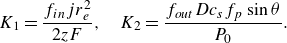 \begin{equation} K_1 = \dfrac {f_{in}jr_e^2}{2zF}, \, \, \, \, \, K_2 = \dfrac {f_{out}D c_{s} f_p \sin \theta }{P_0}. \end{equation}
Because $ (2 + 3 \cos \theta - \cos ^3\theta ) \gt 0,$
the sign of expression (3.13) is determined by the sign of the part in the square brackets on the right-hand side. For the case of
$ (2 + 3 \cos \theta - \cos ^3\theta ) \gt 0,$
the sign of expression (3.13) is determined by the sign of the part in the square brackets on the right-hand side. For the case of $\zeta \leqslant 0$
, this sign is always negative, indicating a stable equilibrium for unpinned bubbles in under-/saturated liquids. However, for larger
$\zeta \leqslant 0$
, this sign is always negative, indicating a stable equilibrium for unpinned bubbles in under-/saturated liquids. However, for larger $\zeta$
, the sign is likely to become positive, in agreement with the statement in Lohse & Zhang (Reference Lohse and Zhang2015a
) that unpinned bubbles are unstable in over-saturated liquids.
$\zeta$
, the sign is likely to become positive, in agreement with the statement in Lohse & Zhang (Reference Lohse and Zhang2015a
) that unpinned bubbles are unstable in over-saturated liquids.
Table 2. Stabilising and destabilising factors for bubbles in an under-/saturated liquid.
For pinned surface bubbles, combining (3.9) and (3.11) leads to (derivation in Appendix (A3))
 \begin{equation} \left [\dfrac { \partial }{\partial \theta } \dfrac {{\rm d}\theta }{{\rm d}t}\right ]_{eq} = \dfrac {M_g }{\rho _g r_{\textit{cl}}^2 C_{2,eq}} (1-\cos \theta _{eq})^2 \left [ \dfrac {2K_4 \gamma }{r_{\textit{cl}}}f_p \cos \theta + K_3 \left (\dfrac {f_{in}}{f_p}\frac {{\rm d}f_p}{{\rm d}\theta } - \frac {\partial f_{in}}{ \partial \theta } \right ) \right ]_{eq}, \end{equation}
with $K_3, \, K_4$
being positive constants at given values of
$K_3, \, K_4$
being positive constants at given values of $j, \, r_e$
and
$j, \, r_e$
and $r_{\textit{cl}}$
 \begin{equation} K_3 = \dfrac { j (r_e^2 - r_{\textit{cl}}^2)}{zFr_{\textit{cl}}}, \, \, \, \, \, K_4 = \dfrac {f_{out}D c_{s} }{P_0}. \end{equation}
The sign of expression (3.15) is determined by the sign of the part in the square brackets on the right-hand side. As will be discussed below (figure 6), for small bubbles ( $r_{\textit{cl}} \sim 1 \, \unicode {x03BC}$
m), the sign is negative when
$r_{\textit{cl}} \sim 1 \, \unicode {x03BC}$
m), the sign is negative when $\theta \gt 90$
° and positive when
$\theta \gt 90$
° and positive when $\theta \lt 90$
°, indicating that the sign is mainly determined by the first term inside the bracket. Thus, only pinned small bubbles of flat shape tend to be stable, while taller caps become unstable by the change of the Laplace pressure (table 2). This generalises the finding in Lohse & Zhang (Reference Lohse and Zhang2015a
) that pinned nanobubbles, which are typically flat, are stable. For larger bubbles, the second term in the bracket may become dominant. Although both
$\theta \lt 90$
°, indicating that the sign is mainly determined by the first term inside the bracket. Thus, only pinned small bubbles of flat shape tend to be stable, while taller caps become unstable by the change of the Laplace pressure (table 2). This generalises the finding in Lohse & Zhang (Reference Lohse and Zhang2015a
) that pinned nanobubbles, which are typically flat, are stable. For larger bubbles, the second term in the bracket may become dominant. Although both ${\rm d}f_p/{\rm d}\theta$
and
${\rm d}f_p/{\rm d}\theta$
and $\partial f_{in} / \partial \theta$
are negative, our calculations reveal that the sign is generally negative for bubbles
$\partial f_{in} / \partial \theta$
are negative, our calculations reveal that the sign is generally negative for bubbles $\sim 50$ $\unicode {x03BC}$
m in size. This corresponds to the fact that the shape factor
$\unicode {x03BC}$
m in size. This corresponds to the fact that the shape factor $f_p$
changes faster than
$f_p$
changes faster than $f_{in}$
with
$f_{in}$
with $\theta$
, as can be seen in Appendix (A1). Therefore, we conclude here that, in under-saturated/saturated bulk electrolytes, bubbles evolving on micro-electrodes in either pinned or unpinned mode may reach a stable equilibrium state. But we remark that under certain conditions, e.g. at large current (Zhang & Lohse Reference Zhang and Lohse2023), an equilibrium state (
$\theta$
, as can be seen in Appendix (A1). Therefore, we conclude here that, in under-saturated/saturated bulk electrolytes, bubbles evolving on micro-electrodes in either pinned or unpinned mode may reach a stable equilibrium state. But we remark that under certain conditions, e.g. at large current (Zhang & Lohse Reference Zhang and Lohse2023), an equilibrium state ( $J_{in}+J_{out}=0$
) may not be achieved at all.
$J_{in}+J_{out}=0$
) may not be achieved at all.
3.2. Numerical simulations
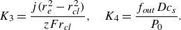
In the following, we investigate the conditions of equilibrium and stability in more detail by combining numerical simulations and theoretical reasoning. Figure 4 shows numerical and theoretical results of the bubble evolution with (dashed lines) and without (dotted lines) the consideration of gas loss into the electrolyte ( $f_{in}, \, f_{out}$
), (3.7) and 3.9. When the applied current density increases, the bubble evolution tends to change from complete dissolution (regime I) towards dynamic equilibrium states (regime II). Unlimited growth until detachment is expected to occur at larger
$f_{in}, \, f_{out}$
), (3.7) and 3.9. When the applied current density increases, the bubble evolution tends to change from complete dissolution (regime I) towards dynamic equilibrium states (regime II). Unlimited growth until detachment is expected to occur at larger $r_b$
and smaller
$r_b$
and smaller $\theta$
, which is outside of the scope of our simulations. We remark that the bubble end state is not influenced by the initial state, see Appendix C. This indicates that convection is not important (
$\theta$
, which is outside of the scope of our simulations. We remark that the bubble end state is not influenced by the initial state, see Appendix C. This indicates that convection is not important ( $Pe=r_b/D \,\boldsymbol\cdot\, {\rm d}r_b/{\rm d}t \ll 1$
), and that bubbles temporarily at different states all tend to converge to the equilibrium state, i.e. the stability condition (3.12) is fulfilled. Because
$Pe=r_b/D \,\boldsymbol\cdot\, {\rm d}r_b/{\rm d}t \ll 1$
), and that bubbles temporarily at different states all tend to converge to the equilibrium state, i.e. the stability condition (3.12) is fulfilled. Because $f_{in}$
is in general smaller than
$f_{in}$
is in general smaller than $f_{out}$
(figure 3), adding them to the original theoretical solution of Zhang & Lohse (Reference Zhang and Lohse2023) causes slower bubble growth and faster dissolution. This improves the agreement with the numerical simulations, especially at smaller currents.
$f_{out}$
(figure 3), adding them to the original theoretical solution of Zhang & Lohse (Reference Zhang and Lohse2023) causes slower bubble growth and faster dissolution. This improves the agreement with the numerical simulations, especially at smaller currents.
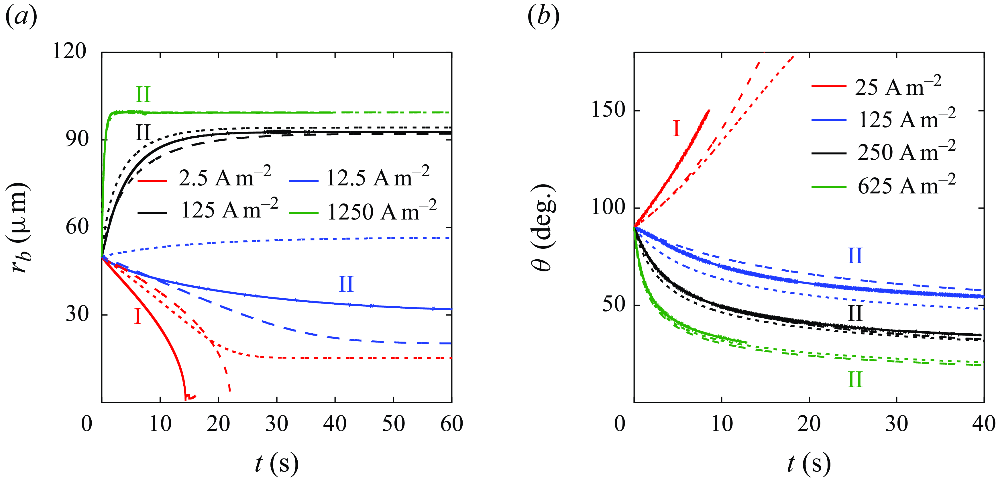
Figure 4. (a) Evolution of the radius of an unpinned bubble, $\theta = 90$
°,
$\theta = 90$
°, $r_e=100\, \unicode {x03BC}$
m,
$r_e=100\, \unicode {x03BC}$
m, $r_{b,{\textit{ini}}}=50 \, \unicode {x03BC}$
m. (b) Evolution of the contact angle of a pinned bubble,
$r_{b,{\textit{ini}}}=50 \, \unicode {x03BC}$
m. (b) Evolution of the contact angle of a pinned bubble, $r_{\textit{cl}}=44 \, \unicode {x03BC}$
m,
$r_{\textit{cl}}=44 \, \unicode {x03BC}$
m, $r_e=55\, \unicode {x03BC}$
m,
$r_e=55\, \unicode {x03BC}$
m, $\theta _{{\textit{ini}}}=90$
°. Regime I: bubble dissolves completely. Regime II: bubble reaches a dynamic equilibrium. Solid lines: simulation. Dashed lines: theoretical solution with
$\theta _{{\textit{ini}}}=90$
°. Regime I: bubble dissolves completely. Regime II: bubble reaches a dynamic equilibrium. Solid lines: simulation. Dashed lines: theoretical solution with $f_{in/out}$
. Dotted lines: theoretical solution without
$f_{in/out}$
. Dotted lines: theoretical solution without $f_{in/out}$
. Note that the simulations are stopped when
$f_{in/out}$
. Note that the simulations are stopped when $\theta \gt$
150° or
$\theta \gt$
150° or $\theta \lt$
30° to avoid numerical difficulties in interface reconstruction.
$\theta \lt$
30° to avoid numerical difficulties in interface reconstruction.
Next, by using the adapted theoretical solution, (3.11), we provide a systematic view of how the final bubble state is influenced by current density, electrode size and wettability. The coloured surface in figure 5(a) represents the contact line radius for unpinned bubbles with a contact angle of 90° when a dynamic equilibrium is reached (regime II). In the white space below the coloured region, no positive root of equation (3.11) exists, i.e. the bubble completely dissolves (regime I). The bubble end states obtained by numerical simulations are added and are found to qualitatively reproduce the theoretical results. As can be seen, the equilibrium bubble size decreases when lowering $r_e$
and
$r_e$
and $j$
. For each current density, there exists a critical electrode size below which bubbles become unstable on the electrode, which decreases at larger
$j$
. For each current density, there exists a critical electrode size below which bubbles become unstable on the electrode, which decreases at larger $j$
. This is because the limited gas influx at the small electrode cannot balance the outflux due to a large Laplace pressure anymore, i.e. it dissolves. The critical
$j$
. This is because the limited gas influx at the small electrode cannot balance the outflux due to a large Laplace pressure anymore, i.e. it dissolves. The critical $r_e$
obtained from the simulations is only slightly larger than for the theoretical solutions. For more hydrophilic electrodes, as shown in figure 5(b) for the case of
$r_e$
obtained from the simulations is only slightly larger than for the theoretical solutions. For more hydrophilic electrodes, as shown in figure 5(b) for the case of $\theta =10$
°,
$\theta =10$
°, $r_{cl,eq}$
becomes smaller, and the dissolution region extends. Note that the results shown here are for the case
$r_{cl,eq}$
becomes smaller, and the dissolution region extends. Note that the results shown here are for the case $\zeta =-1$
. However, a similar behaviour of the bubble evolution was found also for
$\zeta =-1$
. However, a similar behaviour of the bubble evolution was found also for $\zeta =0$
, see Appendix D.
$\zeta =0$
, see Appendix D.
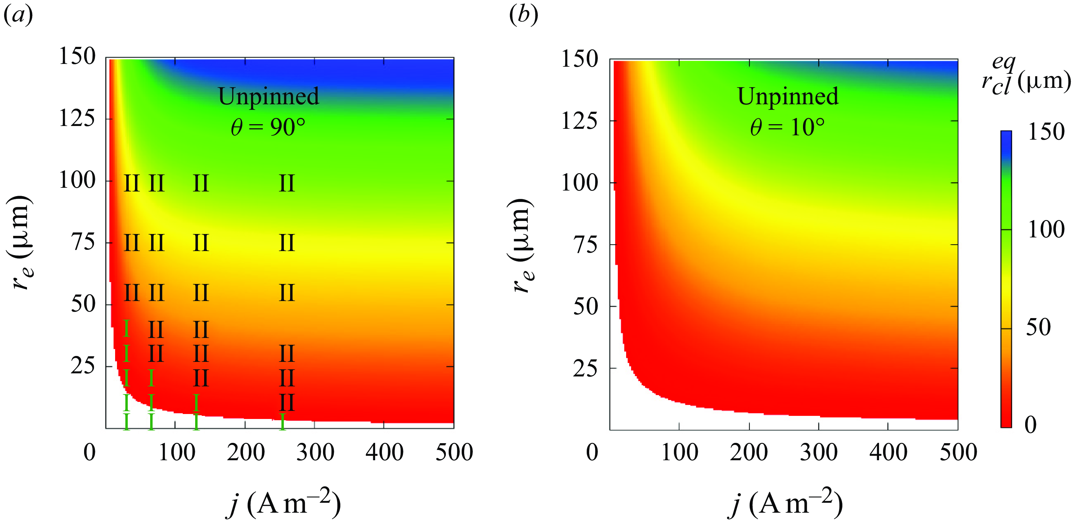
Figure 5. Influence of electrode radius $r_e$
and current density
$r_e$
and current density $j$
on the equilibrium contact line radius
$j$
on the equilibrium contact line radius $r_{\textit{cl}}^{eq}$
of unpinned bubbles when the contact angle is (a) 90° and (b) 10°. Coloured surface: theoretical solution. White area represents complete dissolution. Numerical results of bubble end states (I: complete dissolution; II: dynamic equilibrium) are added in (a).
$r_{\textit{cl}}^{eq}$
of unpinned bubbles when the contact angle is (a) 90° and (b) 10°. Coloured surface: theoretical solution. White area represents complete dissolution. Numerical results of bubble end states (I: complete dissolution; II: dynamic equilibrium) are added in (a).
Figure 6. Influence of electrode radius $r_e$
and current density
$r_e$
and current density $j$
on the equilibrium contact angle
$j$
on the equilibrium contact angle $\theta _{eq}$
of pinned bubbles with (a)
$\theta _{eq}$
of pinned bubbles with (a) $r_{\textit{cl}}=50\,\unicode {x03BC}$
m or (b)
$r_{\textit{cl}}=50\,\unicode {x03BC}$
m or (b) $r_{\textit{cl}}=1\,\unicode {x03BC}$
m. Coloured surface: theoretical solution. White or grey areas represent complete dissolution or unlimited growth. Numerical results of bubble end states (I: complete dissolution; II: dynamic equilibrium) are added in (a). The black curve in (b) marks
$r_{\textit{cl}}=1\,\unicode {x03BC}$
m. Coloured surface: theoretical solution. White or grey areas represent complete dissolution or unlimited growth. Numerical results of bubble end states (I: complete dissolution; II: dynamic equilibrium) are added in (a). The black curve in (b) marks $ [ \partial ({\rm d}\theta / {\rm d}t) / \partial \theta ]_{eq} =0$
, which is not visible in (a) where the expression is always negative.
$ [ \partial ({\rm d}\theta / {\rm d}t) / \partial \theta ]_{eq} =0$
, which is not visible in (a) where the expression is always negative.
Figure 6 shows the final contact angle of pinned bubbles with pinning radii of 50 $\unicode {x03BC}$
m (a) and 1
$\unicode {x03BC}$
m (a) and 1 $\unicode {x03BC}$
m (b). The white space below the coloured region represents the cases of complete dissolution (
$\unicode {x03BC}$
m (b). The white space below the coloured region represents the cases of complete dissolution ( $\theta \rightarrow 180$
°), and the upper grey area represents unlimited growth (
$\theta \rightarrow 180$
°), and the upper grey area represents unlimited growth ( $\theta \rightarrow 0$
°). As can further be seen, smaller
$\theta \rightarrow 0$
°). As can further be seen, smaller $r_e$
and lower
$r_e$
and lower $j$
lead to more flat bubbles. Such a change in bubble shape reduces the surface available for
$j$
lead to more flat bubbles. Such a change in bubble shape reduces the surface available for $J_{out}$
, thus maintaining the equilibrium at higher Laplace pressure and slower gas production. For each current density, also there exists here a critical
$J_{out}$
, thus maintaining the equilibrium at higher Laplace pressure and slower gas production. For each current density, also there exists here a critical $r_e$
below which bubbles always dissolve, which decreases with increasing
$r_e$
below which bubbles always dissolve, which decreases with increasing $j$
. We remark that such a critical electrode size only exists for under-saturated liquids (
$j$
. We remark that such a critical electrode size only exists for under-saturated liquids ( $\zeta \lt 0$
), where the influx due to gas production then becomes lower than the outflux. This is not the case for saturated liquids (
$\zeta \lt 0$
), where the influx due to gas production then becomes lower than the outflux. This is not the case for saturated liquids ( $\zeta =0$
), where
$\zeta =0$
), where $J_{out}$
becomes independent of the size of the bubble (see (3.2)). Here, for smaller electrodes, the bubble can always flatten its shape towards
$J_{out}$
becomes independent of the size of the bubble (see (3.2)). Here, for smaller electrodes, the bubble can always flatten its shape towards $\theta =180$
° to reduce
$\theta =180$
° to reduce $J_{out}$
in order to balance a smaller
$J_{out}$
in order to balance a smaller $J_{in}$
.
$J_{in}$
.
A bubble does not necessarily stay stable after an equilibrium state has temporarily been reached. As mentioned above, unpinned bubbles are always stable in liquids of $\zeta \leqslant 0$
(3.13). For pinned bubbles of
$\zeta \leqslant 0$
(3.13). For pinned bubbles of $r_{\textit{cl}}=50\, \unicode {x03BC}$
m, the sign of
$r_{\textit{cl}}=50\, \unicode {x03BC}$
m, the sign of $ [ ({ \partial }/{\partial \theta }) ({{\rm d}\theta }/{{\rm d}t} ]_{eq}$
(equation (3.15)) is found to be negative, i.e. the bubbles have a stable equilibrium. For smaller bubbles of
$ [ ({ \partial }/{\partial \theta }) ({{\rm d}\theta }/{{\rm d}t} ]_{eq}$
(equation (3.15)) is found to be negative, i.e. the bubbles have a stable equilibrium. For smaller bubbles of $r_{\textit{cl}}=1\, \unicode {x03BC}$
m, we plot the isoline
$r_{\textit{cl}}=1\, \unicode {x03BC}$
m, we plot the isoline $ [ ({ \partial }/{\partial \theta }) ({{\rm d}\theta }/{{\rm d}t}) ]_{eq} =0$
as a black solid line in figure 6(b). We find that the sign of this expression is negative for
$ [ ({ \partial }/{\partial \theta }) ({{\rm d}\theta }/{{\rm d}t}) ]_{eq} =0$
as a black solid line in figure 6(b). We find that the sign of this expression is negative for $\theta \gt 90$
° and positive for
$\theta \gt 90$
° and positive for $\theta \lt 90$
° in general. This confirms the analysis below (3.16). More details on the distribution of the sign can be found in Appendix (A3).
$\theta \lt 90$
° in general. This confirms the analysis below (3.16). More details on the distribution of the sign can be found in Appendix (A3).
We further note that, for all the simulations performed in this work, the stable bubble equilibra found correspond to Damköhler numbers ranging mainly between 0.1 and 1, which a posteriori justifies our approach of extending the theory of the reaction-controlled growth. For more details please see Appendix E.
3.3. Impact on reaction efficiency
Finally, we discuss how to design the electrode to effectively regulate the bubble equilibrium, aiming to reduce electrode blockage and thus related energy losses. For an unpinned bubble, its contact radius determines the active area of the electrode for reaction. Figure 7(a) shows how the fraction of the electrode surface covered by the bubble changes with the current density applied ( $j_{app}$
). In general, lower
$j_{app}$
). In general, lower $j_{app}$
, smaller and more hydrophilic electrodes could reduce the bubble coverage. Figure 7(b) shows the current density averaged over the whole electrode area,
$j_{app}$
, smaller and more hydrophilic electrodes could reduce the bubble coverage. Figure 7(b) shows the current density averaged over the whole electrode area, $j_{avg}$
, as a function of
$j_{avg}$
, as a function of $j_{app}$
, which sheds insight onto the experimentally measurable
$j_{app}$
, which sheds insight onto the experimentally measurable $\textrm{current}-\textrm{potential}$
curve (Bard et al. Reference Bard, Faulkner and White2022): an indicator of the energy transfer efficiency of the electrolysis. When
$\textrm{current}-\textrm{potential}$
curve (Bard et al. Reference Bard, Faulkner and White2022): an indicator of the energy transfer efficiency of the electrolysis. When $j_{app}$
increases,
$j_{app}$
increases, $j_{avg}$
first increases then levels off, and even slightly decreases. Smaller and hydrophilic electrodes are beneficial for enhancing the efficiency. These trends correlate with lower bubble coverage on the electrode. Further, when the electrode is increasingly blocked by the bubble, the electric current lines will concentrate near the electrode edge. This may lead to a temperature hotspot, causing a thermal Marangoni force that retards the bubble detachment (Hossain et al. Reference Hossain, Mutschke, Bashkatov and Eckert2020). If a bubble is pinned by geometrical or chemical surface heterogeneities, the bubble coverage of the electrode is pre-defined, and the reaction efficiency can only be influenced by the bubble shape. For smaller
$j_{avg}$
first increases then levels off, and even slightly decreases. Smaller and hydrophilic electrodes are beneficial for enhancing the efficiency. These trends correlate with lower bubble coverage on the electrode. Further, when the electrode is increasingly blocked by the bubble, the electric current lines will concentrate near the electrode edge. This may lead to a temperature hotspot, causing a thermal Marangoni force that retards the bubble detachment (Hossain et al. Reference Hossain, Mutschke, Bashkatov and Eckert2020). If a bubble is pinned by geometrical or chemical surface heterogeneities, the bubble coverage of the electrode is pre-defined, and the reaction efficiency can only be influenced by the bubble shape. For smaller $\theta$
, the electric current lines will be more distorted near the bubble, resulting in a stronger shielding effect and larger ohmic loss. As can be seen in figure 5,
$\theta$
, the electric current lines will be more distorted near the bubble, resulting in a stronger shielding effect and larger ohmic loss. As can be seen in figure 5, $\theta _{eq}$
increases when
$\theta _{eq}$
increases when $r_e, r_{\textit{cl}}$
and
$r_e, r_{\textit{cl}}$
and $j_{app}$
decrease. This again indicates the advantage of using electrodes of smaller size or electrodes structured with an array of nano-/micrometre-sized catalytic spots.
$j_{app}$
decrease. This again indicates the advantage of using electrodes of smaller size or electrodes structured with an array of nano-/micrometre-sized catalytic spots.
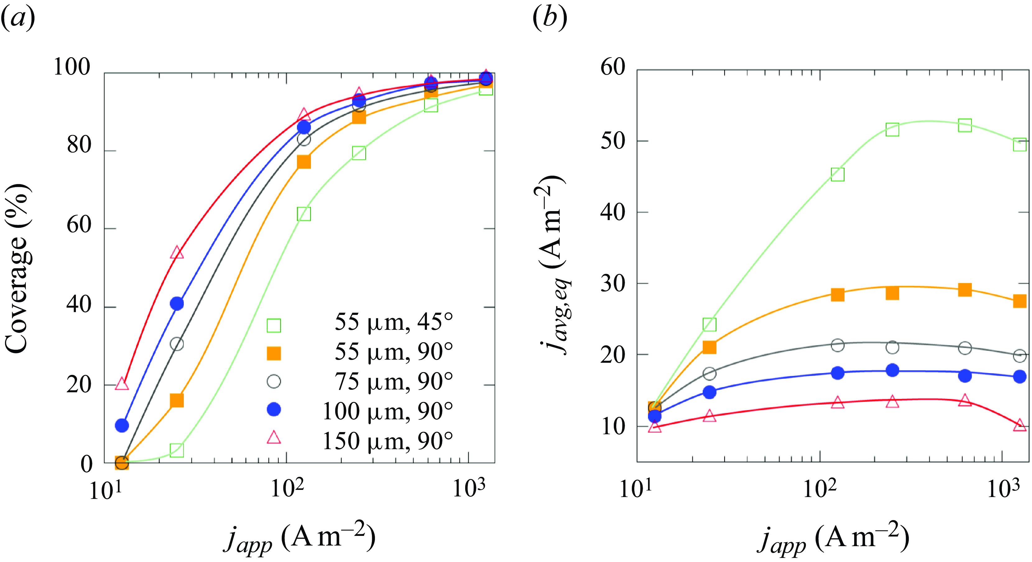
Figure 7. (a) Electrode coverage and (b) current density averaged over the whole electrode surface area for unpinned bubbles at equilibrium for micro-electrodes of different size and wettability, $r_{b,{\textit{ini}}}=50 \, \unicode {x03BC}$
m.
$r_{b,{\textit{ini}}}=50 \, \unicode {x03BC}$
m.
4. Conclusions and outlook
We studied the equilibrium and stability of gas bubbles evolving at micro-electrodes using direct numerical simulations and theoretical analysis by adapting an existing theoretical model for the reaction-controlled mode. At micro-electrodes, both pinned and unpinned bubbles may reach a dynamic equilibrium state, at which the in- and outfluxes of gas across the bubble surface counterbalance each other. The equilibrium states are characterised by Damköhler numbers smaller than or around 1. In under- and saturated bulk electrolytes, this equilibrium is always stable for unpinned bubbles. Under contact line pinning, it is stable for flat nano-bubbles with a contact angle larger than 90° and for micro-bubbles in general. Both numerical and theoretical solutions suggest a critical electrode size, below which bubbles in undersaturated (pinned/unpinned) or saturated (unpinned) liquids will eventually dissolve.
We note that our investigation is limited to the axisymmetric cases where the initial bubble nucleus resides at the centre of the microelectrode. Therefore, asymmetric nucleation and disturbances have to be studied in future work. We further remark that there could be situations that the pinned and unpinned cases considered in this work cannot cover. The modes we considered are idealisations, as we neglect small movements of the contact line during pinning and small changes of the contact angle during unpinned growth. Further, the bubble may also evolve in both regimes, with a short transitional period in between, where both the contact angle and contact line are changing in time (Li et al. Reference Li, Matkarimov, Xiao, Liu and Yang2023a ). The instant of the transition from the pinned to the unpinned mode on a specific surface depends on its wetting properties. In general, de-pinning occurs earlier on more hydrophobic surfaces. If de-pinning occurs before the bubble has reached an equilibrium, stable pinned states will not be achieved. Besides, on rough surfaces, expanding bubbles may also become re-pinned again at surface tips before having reached an equilibrium contact line radius. Therefore, what stable bubble states can be observed on micro-electrodes beside the process parameters may also depend on the dynamic wetting property of the surface, and awaits a further clarification in future studies.
The specifics of the bubble dynamics at micro-electrodes unveiled in this work give support to recent experimental observations of stationary bubbles and bubble dissolution (Suvira et al. Reference Suvira, Ahuja, Lovre, Singh, Draher and Zhang2023). We hope that the present findings will stimulate work towards further validation. Our findings may also contribute to future efficiency enhancements of water electrolysis by using hydrophilic electrodes of smaller size or electrodes structured with an array of nano-/micrometre-sized catalytic spots at moderate current densities.
Acknowledgements
We gratefully acknowledge discussions with C. Chen and Y. Ma.
Funding
Financial support by the National Natural Science Foundation of China, grant nos. 22309007 and 11988102, the Federal Ministry of Education and Research within the project H2Giga-SINEWAVE, grant no. 03HY123E and the Maria Reiche Postdoctoral Fellowships of the TU Dresden funded by the State of Saxony and the Federal and State Program for Women Professors (Professorinnenprogramm) are greatly acknowledged.
Declaration of interests
The authors report no conflict of interest.
Appendix A. Details of expressions and derivations
A.1 The variables $f_{in}, f_{out}, f_p$

According to figure 3, only small variations can be observed when the electrode size changes. The dependence of $f_{out}$
on the contact angle is also negligibly small. Therefore, we simplify the theoretical solutions by using fitting functions for
$f_{out}$
on the contact angle is also negligibly small. Therefore, we simplify the theoretical solutions by using fitting functions for $f_{in}$
and
$f_{in}$
and $f_{out}$
. These read
$f_{out}$
. These read
 \begin{align} f_{in}(j,\theta )& = 1.378 (-0.0037 \theta + 1.066)\,\boldsymbol\cdot\, (0.184 ln(j) - 0.296),\end{align}
 \begin{align} f_{out}(j) & = 1.027 (0.075 ln(j) +0.441).\end{align}
Here, a simple linear fitting of $f_{in}$
and
$f_{in}$
and $f_{out}$
vs.
$f_{out}$
vs. $\theta$
and
$\theta$
and $ln(j)$
was chosen, which already gives a coefficient of determination (
$ln(j)$
was chosen, which already gives a coefficient of determination ( $R^2$
) of
$R^2$
) of $\sim$
0.95. The shape factor
$\sim$
0.95. The shape factor $f_p$
used to compute
$f_p$
used to compute $J_{out}$
is defined as follows (Popov Reference Popov2005):
$J_{out}$
is defined as follows (Popov Reference Popov2005):
 \begin{equation} f_p(\theta ) = \dfrac {\mathrm{sin} \theta }{1 - \mathrm{cos} \theta } + 4 \int _{0}^{\infty } \dfrac {1+\mathrm{cosh} [ 2 (\pi - \theta ) \tau ] }{\mathrm{sinh} (2 \pi \tau )} \mathrm{tanh}(\theta \tau )\,{\rm d}\tau, \end{equation}
with $\theta$
denoting the water-side contact angle. It can be numerically approximated by the fitting function
$\theta$
denoting the water-side contact angle. It can be numerically approximated by the fitting function $f_p(\theta )=112.55 \theta ^{-0.884}$
. Figure 8 compares the behaviours of
$f_p(\theta )=112.55 \theta ^{-0.884}$
. Figure 8 compares the behaviours of $f_{in}$
and
$f_{in}$
and $f_p$
, calculated either by (A3) or the fitting function, versus
$f_p$
, calculated either by (A3) or the fitting function, versus $\theta$
. We remark that (A3) has asymptotic solutions for
$\theta$
. We remark that (A3) has asymptotic solutions for $\theta = 90$
° and 180°, which equal to 2 and
$\theta = 90$
° and 180°, which equal to 2 and $4/\pi$
, respectively (Wilson & D’Ambrosio Reference Wilson and D‘Ambrosio2023). This gives a difference of
$4/\pi$
, respectively (Wilson & D’Ambrosio Reference Wilson and D‘Ambrosio2023). This gives a difference of $5 \,\%-10$
% compared with the result based on the fitting function.
$5 \,\%-10$
% compared with the result based on the fitting function.
In general, all factors decrease with increased $\theta$
, among which the Popov factor
$\theta$
, among which the Popov factor $f_p$
changes fastest. The influence of
$f_p$
changes fastest. The influence of $\theta$
on
$\theta$
on $f_{out}$
is only minor and is neglected in the derivation of bubble stability.
$f_{out}$
is only minor and is neglected in the derivation of bubble stability.
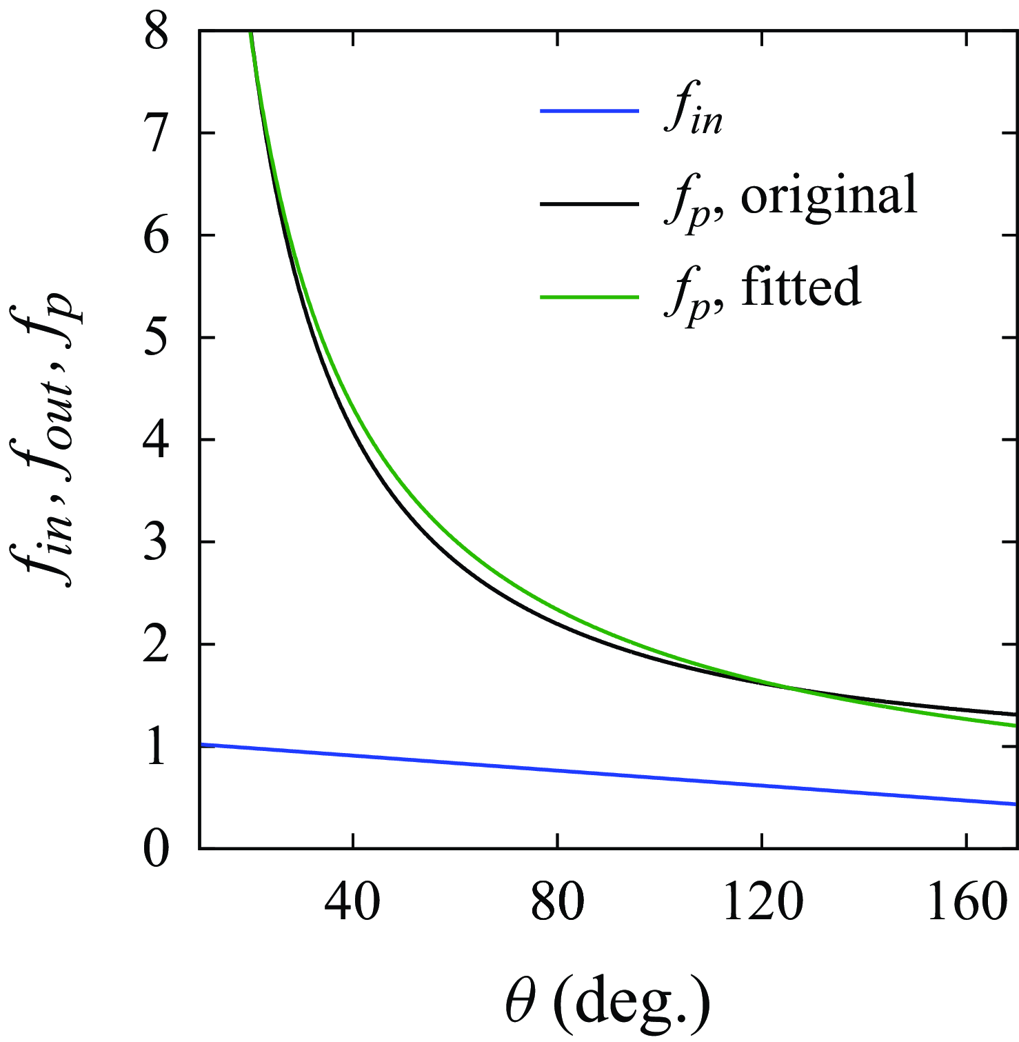
Figure 8. Comparison of $f_{in}$
(
$f_{in}$
( $j=250$
A m
$j=250$
A m ${^-}^2$
) and
${^-}^2$
) and $f_p$
depending on the water-side contact angle.
$f_p$
depending on the water-side contact angle.
A.2 Influence of varying gas density
As mentioned in § 3.1, the dependence of gas density on the pressure may influence the bubble dynamics, especially at nano- and micro-scales. Here, we present results of (3.7) and (3.9) for unpinned (figure 9) and pinned (figure 10) bubbles. As can be seen, the enhanced actual gas density (equation (3.5)) may slow down the initial growth speed for bubbles smaller than 5 $\unicode {x03BC}$
m, which corresponds to a maximal relative density change
$\unicode {x03BC}$
m, which corresponds to a maximal relative density change $\Delta \rho _g/\rho _{g0}$
of 29 %, and a minimal compressibility term (
$\Delta \rho _g/\rho _{g0}$
of 29 %, and a minimal compressibility term ( $C_1$
or
$C_1$
or $C_2$
) of
$C_2$
) of $\sim$
0.9. We remark that the equilibrium bubble state is not influenced, as evidenced also by (3.11). For most cases considered in this work, the influence of varying gas density can be safely neglected.
$\sim$
0.9. We remark that the equilibrium bubble state is not influenced, as evidenced also by (3.11). For most cases considered in this work, the influence of varying gas density can be safely neglected.
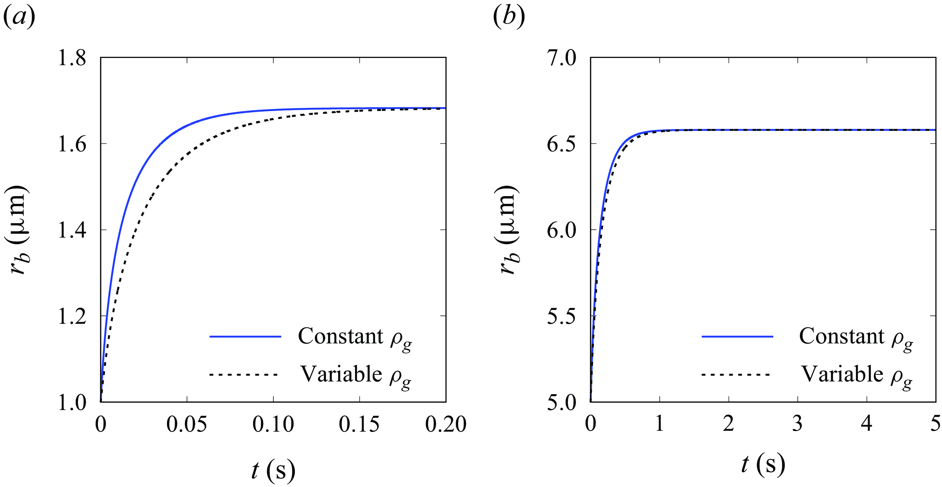
Figure 9. Influence of variable gas density on the evolution of the radius of unpinned bubbles with $\theta = 90$
° and
$\theta = 90$
° and $j=250$
A m
$j=250$
A m ${^-}^2$
. Panels show (a)
${^-}^2$
. Panels show (a) $r_{b,{\textit{ini}}}=1 \, \unicode {x03BC}$
m,
$r_{b,{\textit{ini}}}=1 \, \unicode {x03BC}$
m, $r_e=5 \, \unicode {x03BC}$
m,
$r_e=5 \, \unicode {x03BC}$
m, $[\Delta \rho _g/\rho _{g0}]_{{\textit{max}}} = 146\,\%$
,
$[\Delta \rho _g/\rho _{g0}]_{{\textit{max}}} = 146\,\%$
, $[C_1]_{{\textit{min}}} = 0.8$
and (b)
$[C_1]_{{\textit{min}}} = 0.8$
and (b) $r_{b,{\textit{ini}}}=5 \, \unicode {x03BC}$
m,
$r_{b,{\textit{ini}}}=5 \, \unicode {x03BC}$
m, $r_e=10 \, \unicode {x03BC}$
m,
$r_e=10 \, \unicode {x03BC}$
m, $[\Delta \rho _g/\rho _{g0}]_{{\textit{max}}} = 29\,\%$
,
$[\Delta \rho _g/\rho _{g0}]_{{\textit{max}}} = 29\,\%$
, $[C_1]_{{\textit{min}}} = 0.92$
.
$[C_1]_{{\textit{min}}} = 0.92$
.
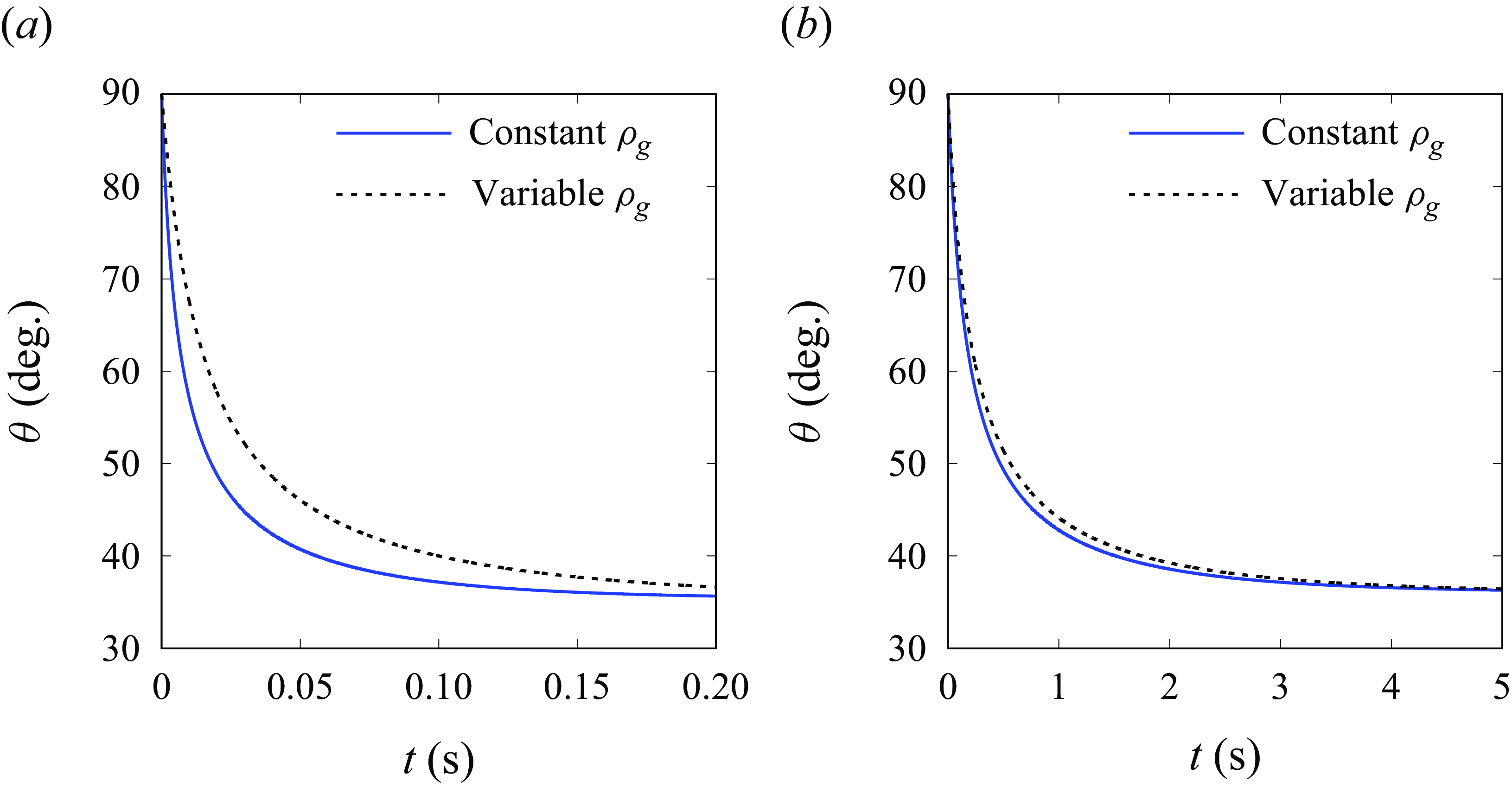
Figure 10. Influence of variable gas density on the evolution of the contact angle of pinned bubbles with $\theta _{{\textit{ini}}}=90$
° and
$\theta _{{\textit{ini}}}=90$
° and $j=250$
A m
$j=250$
A m ${^-}^2$
. Panels show (a)
${^-}^2$
. Panels show (a) $r_{cl,{\textit{ini}}}=1 \, \unicode {x03BC}$
m,
$r_{cl,{\textit{ini}}}=1 \, \unicode {x03BC}$
m, $r_e=5 \, \unicode {x03BC}$
m,
$r_e=5 \, \unicode {x03BC}$
m, $[\Delta \rho _g/\rho _{g0}]_{{\textit{max}}} = 146\,\%$
,
$[\Delta \rho _g/\rho _{g0}]_{{\textit{max}}} = 146\,\%$
, $[C_2]_{{\textit{min}}} = 0.85$
and (b)
$[C_2]_{{\textit{min}}} = 0.85$
and (b) $r_{cl,{\textit{ini}}}=5 \, \unicode {x03BC}$
m,
$r_{cl,{\textit{ini}}}=5 \, \unicode {x03BC}$
m, $r_e=10 \, \unicode {x03BC}$
m,
$r_e=10 \, \unicode {x03BC}$
m, $[\Delta \rho _g/\rho _{g0}]_{{\textit{max}}} = 29\,\%$
,
$[\Delta \rho _g/\rho _{g0}]_{{\textit{max}}} = 29\,\%$
, $[C_2]_{{\textit{min}}} = 0.95$
.
$[C_2]_{{\textit{min}}} = 0.95$
.
A.3 Derivations of bubble stability
In the following, we derive the stability conditions (Lohse & Zhang Reference Lohse and Zhang2015a )
 \begin{equation} \left [\dfrac { \partial }{\partial r_b}\frac {{\rm d}r_b}{{\rm d}t}\right ]_{eq} \lt 0, \, \, \, \, \, \left [\dfrac { \partial }{\partial \theta } \frac {{\rm d}\theta }{{\rm d}t}\right ]_{eq} \lt 0, \end{equation}
for the bubbles that have reached an equilibrium.
For the unpinned bubbles, based on (3.7), the temporal change of the bubble radius can be expressed as
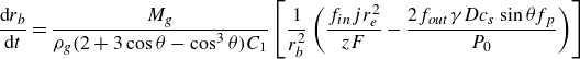 \begin{align} \dfrac {{\rm d}r_b}{{\rm d}t} &= \dfrac {M_g }{\rho _g ( 2 + 3 \cos \theta - \cos ^3\theta ) C_1 } \left [ \frac {1}{r_b^2}\left ( \dfrac {f_{in}jr_e^2}{zF} - \dfrac {2 f_{out} \gamma D c_{s} \sin \theta f_p }{P_0} \right ) \right ]\\ \nonumber \end{align}
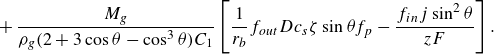 \begin{align} &\quad + \dfrac {M_g }{\rho _g ( 2 + 3 \cos \theta - \cos ^3\theta ) C_1 } \left [ \frac {1}{r_b} f_{out} D c_{s} \zeta \sin \theta f_p - \dfrac {f_{in}j \sin ^2\theta }{zF}\right ] . \end{align}
To ease the derivation, we define variables $K_1,\, K_2$
that are positive constant values during each bubble evolution event with constant
$K_1,\, K_2$
that are positive constant values during each bubble evolution event with constant $j, \, r_e$
and
$j, \, r_e$
and $\theta$
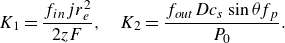 \begin{equation} K_1 = \dfrac {f_{in}jr_e^2}{2zF}, \, \, \, \, \, K_2 = \dfrac {f_{out}D c_{s} \sin \theta f_p }{P_0}. \end{equation}
At equilibrium, combining (3.11) and A7, we obtain
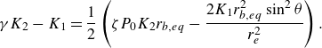 \begin{equation} \gamma K_2 - K_1 = \frac {1}{2}\left ( \zeta P_0 K_2 r_{b,eq} - \dfrac {2K_1 r_{b,eq}^2 \sin ^2 \theta }{r_e^2} \right ). \end{equation}
Applying the quotient rule and the equilibrium condition (A8), the partial derivative of (A6) can be expressed as follows:
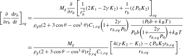 \begin{align} \left [ \dfrac { \partial }{\partial r_b} \frac {{\rm d}r_b}{{\rm d}t}\right ]_{eq} &=\dfrac {M_g \dfrac {\partial }{\partial r_b} \left [ \dfrac {1}{r_b^2}(2K_1 - 2\gamma K_2) + \dfrac {1}{r_b}(\zeta P_0 K_2) \right ]_{eq} }{ \rho _{g0} ( 2 + 3 \cos \theta - \cos ^3\theta ) C_{1,eq}\!\left (\!1 \!+\! \dfrac {2 \gamma }{r_{b,eq}P_0}\!\right ) \dfrac { \left(P_0 b + k_B T\right)}{P_0 b\! \left (\!1\! +\! \dfrac {2 \gamma }{r_{b,eq} P_0}\!\right )\! +\! k_B T}}\nonumber \\ &=\dfrac {M_g }{\rho _g ( 2 + 3 \cos \theta - \cos ^3\theta )r_{b,eq}^2 C_{1,eq} } \left [ \frac {4(\gamma K_2 - K_1) - \zeta P_0 K_2 r_{b,eq}}{r_{b,eq}} \right ]. \end{align}
which can be further simplified using (A8) again
 \begin{equation} \left [\dfrac { \partial }{\partial r_b} \frac {{\rm d}r_b}{{\rm d}t} \right ]_{eq}=\dfrac {M_g }{\rho _g ( 2 + 3 \cos \theta - \cos ^3\theta ) r_{b,eq}^2 C_{1,eq}} \left [ \zeta P_0 K_2 - \dfrac {4K_1 r_{b,eq} \sin ^2 \theta }{r_e^2} \right ]. \end{equation}
Because $ (2 + 3 \cos \theta - \cos ^3\theta ) \gt 0$
,
$ (2 + 3 \cos \theta - \cos ^3\theta ) \gt 0$
, $C_{1,eq}\gt 0$
, the sign of
$C_{1,eq}\gt 0$
, the sign of $ [ ({\partial }/{ \partial r_b}) ({{\rm d}r_b}/{{\rm d}t}) ]_{eq}$
is determined by the sign of the square bracket on the right-hand side of (A10)
$ [ ({\partial }/{ \partial r_b}) ({{\rm d}r_b}/{{\rm d}t}) ]_{eq}$
is determined by the sign of the square bracket on the right-hand side of (A10)
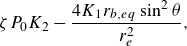 \begin{equation} \zeta P_0 K_2 - \dfrac {4K_1 r_{b,eq} \sin ^2 \theta }{r_e^2}, \end{equation}
which is negative if $\zeta \leqslant 0$
. We remark that this expression can also be readily applied to bubbles on non-reactive surfaces by setting
$\zeta \leqslant 0$
. We remark that this expression can also be readily applied to bubbles on non-reactive surfaces by setting $K_1=0$
,
$K_1=0$
, $f_{out}=1$
.
$f_{out}=1$
.
For a pinned bubble, based on (3.9), we express the temporal change of the water-side contact angle as follows:
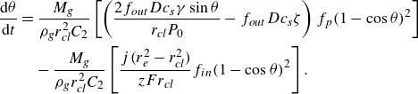 \begin{align} \dfrac {{\rm d}\theta }{{\rm d}t} &= \dfrac {M_g }{\rho _g r_{\textit{cl}}^2 C_2} \left [ \left ( \dfrac { 2f_{out}Dc_{s}\gamma \sin \theta }{r_{\textit{cl}}P_0} - f_{out} D c_{s} \zeta \right ) f_p (1-\cos \theta )^2 \right ]\nonumber\\ & \quad - \dfrac {M_g }{\rho _g r_{\textit{cl}}^2 C_2} \left [ \dfrac { j (r_e^2 - r_{\textit{cl}}^2)}{zFr_{\textit{cl}}} f_{in} (1-\cos \theta )^2 \right ]. \end{align}
Defining variables that are positive constants during each bubble evolution event with constant $j, \, r_e$
and
$j, \, r_e$
and $r_{\textit{cl}}$
 \begin{equation} K_3 = \dfrac { j (r_e^2 - r_{\textit{cl}}^2)}{zFr_{\textit{cl}}}, \, \, \, \, \, K_4 = \dfrac {f_{out}D c_{s} }{P_0}. \end{equation}
At equilibrium, combining (3.11) and (A13), we obtain
 \begin{equation} \left (2 K_4\gamma \sin \theta _{eq} - K_4 P_0\zeta r_{\textit{cl}} \right )f_p = K_3 r_{\textit{cl}} f_{in}. \end{equation}
The partial derivative of (A12) then becomes
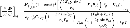 \begin{equation} \left [ \dfrac { \partial }{\partial \theta } \dfrac {{\rm d}\theta }{{\rm d}t}\right ]_{eq} = \dfrac {M_g \dfrac {\partial }{\partial \theta } (1-\cos \theta )^2 \left [ \left (\dfrac {2 K_4 \gamma \sin \theta }{r_{\textit{cl}}} - K_4 P_0 \zeta \right )f_p - K_3 f_{in} \right ]_{eq}}{\rho _{g0} r_{\textit{cl}}^2 C_{2,eq} \left (1 + \dfrac {2 \gamma \sin \theta _{eq} }{r_{\textit{cl}}P_0}\right ) \dfrac { (P_0 b + k_B T)}{P_0 b \left (1 + \dfrac {2 \gamma \sin \theta _{eq}}{r_{\textit{cl}} P_0}\right ) + k_B T} } . \end{equation}
This can be further simplified as
 \begin{align} \left [\dfrac { \partial }{\partial \theta } \dfrac {{\rm d}\theta }{{\rm d}t}\right ]_{eq} &=\dfrac {M_g }{\rho _g r_{\textit{cl}}^2 C_{2,eq}} (1-\cos \theta _{eq})^2 \frac {\partial }{\partial \theta } \left [ \left (\dfrac {2 K_4 \gamma \sin \theta }{r_{\textit{cl}}} - K_4 P_0 \zeta \right )f_p - K_3 f_{in} \right ]_{eq}\nonumber \\ &= \dfrac {M_g }{\rho _g r_{\textit{cl}}^2 C_{2,eq}} (1-\cos \theta _{eq})^2 \left [ \dfrac {2K_4 \gamma }{r_{\textit{cl}}}f_p\cos \theta + K_3 \left (\dfrac {f_{in}}{f_p}\frac {{\rm d}f_p}{{\rm d}\theta } - \frac {\partial f_{in}}{ \partial \theta } \right ) \right ]_{eq}. \end{align}
The sign of $ [ ({ \partial }/{\partial \theta }) ({{\rm d}\theta }/{{\rm d}t}) ]_{eq}$
is determined by the sign of the square bracket on the right-hand side of (A16)
$ [ ({ \partial }/{\partial \theta }) ({{\rm d}\theta }/{{\rm d}t}) ]_{eq}$
is determined by the sign of the square bracket on the right-hand side of (A16)
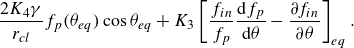 \begin{equation} \dfrac {2K_4 \gamma }{r_{\textit{cl}}} f_p (\theta _{eq})\cos \theta _{eq} + K_3 \left [\dfrac {f_{in}}{f_p}\frac {{\rm d}f_p}{{\rm d}\theta } - \frac {\partial f_{in}}{ \partial \theta } \right ]_{eq}. \end{equation}
Unlike the unpinned case, where the sign of $ [ \partial ({\rm d} r_b / {\rm d}t) / \partial r_b ]_{eq}$
is clearly negative if
$ [ \partial ({\rm d} r_b / {\rm d}t) / \partial r_b ]_{eq}$
is clearly negative if $\zeta \leqslant 0$
(expression (A11)), in the pinned case the stability behaviour is more complex. As shown in figure 11, for a relatively large contact radius (50
$\zeta \leqslant 0$
(expression (A11)), in the pinned case the stability behaviour is more complex. As shown in figure 11, for a relatively large contact radius (50 $\unicode {x03BC}$
m), the sign of expression (A17) and thus of (A16) is negative in the parameter range considered. Thus, larger pinned bubbles at dynamic equilibrium are stable. For a smaller pinned bubble of 1
$\unicode {x03BC}$
m), the sign of expression (A17) and thus of (A16) is negative in the parameter range considered. Thus, larger pinned bubbles at dynamic equilibrium are stable. For a smaller pinned bubble of 1 $\unicode {x03BC}$
m, the sign of expression (A17) is found to be positive in the upper equilibrium area where
$\unicode {x03BC}$
m, the sign of expression (A17) is found to be positive in the upper equilibrium area where $\theta _{eq}\gt 90$
° according to figure 6, and is found to be negative in the lower equilibrium area where
$\theta _{eq}\gt 90$
° according to figure 6, and is found to be negative in the lower equilibrium area where $\theta _{eq}\lt 90$
°. Thus, only in the latter part the dynamic equilibrium is stable. Considering expression (A17), we note that its first term is positive and negative when
$\theta _{eq}\lt 90$
°. Thus, only in the latter part the dynamic equilibrium is stable. Considering expression (A17), we note that its first term is positive and negative when $\theta$
is smaller and larger than 90°, respectively. Its second term can be assumed to be negative, because
$\theta$
is smaller and larger than 90°, respectively. Its second term can be assumed to be negative, because $f_{p}$
decreases faster with
$f_{p}$
decreases faster with $\theta$
than
$\theta$
than $f_{in}$
(see figure 8). Therefore, the sign of
$f_{in}$
(see figure 8). Therefore, the sign of $ [ \partial ({\rm d}\theta / {\rm d}t) / \partial \theta ]_{eq}$
for small bubbles is determined by the first term of expression (A17) originating from the Laplace pressure, and for larger bubbles it is determined by the second term originating from the bubble shape. Note that, for bubbles on non-reactive surfaces,
$ [ \partial ({\rm d}\theta / {\rm d}t) / \partial \theta ]_{eq}$
for small bubbles is determined by the first term of expression (A17) originating from the Laplace pressure, and for larger bubbles it is determined by the second term originating from the bubble shape. Note that, for bubbles on non-reactive surfaces, $j=0, \, K_3=0$
, so that this expression is only determined by the first term. All results of the theoretical solution shown in the figures were computed by using Matlab.
$j=0, \, K_3=0$
, so that this expression is only determined by the first term. All results of the theoretical solution shown in the figures were computed by using Matlab.
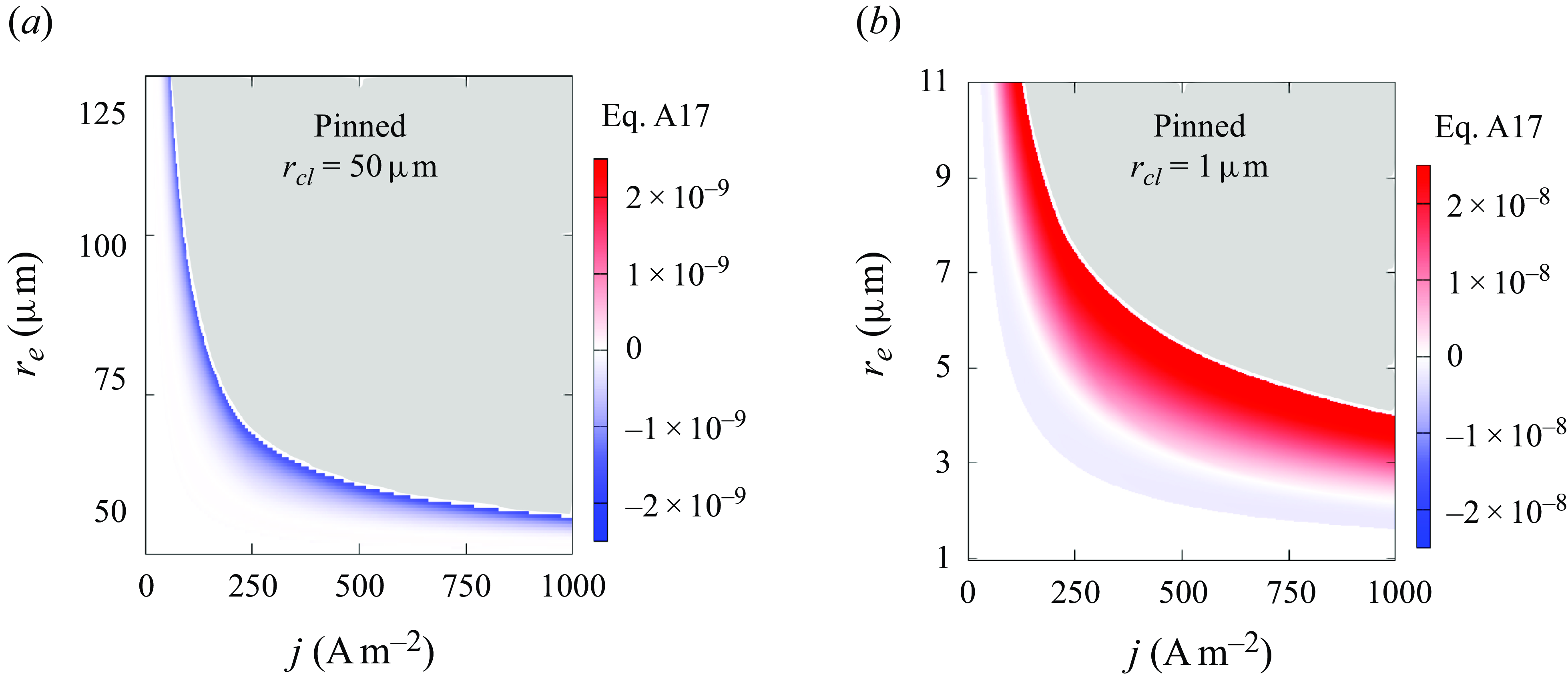
Figure 11. Value of expression (A17) for two pinned bubbles of different contact radius at dynamic equilibrium. The white and grey areas indicate bubble dissolution and unlimited growth.
Appendix B. Variation of surface slip and diffusion coefficient
As can be seen in figure 12, changing the boundary condition at the substrate from no slip to free slip does not change the bubble evolution process. Besides, using different values of manually increased diffusion coefficients does not affect the results. This requires us to re-scale time according to the ratio of the increased to real diffusion coefficient. The enlarged diffusion coefficient must not impair the dominance of surface tension during bubble growth (Han et al. Reference Han, Haung, Eckert and Mutschke2025).
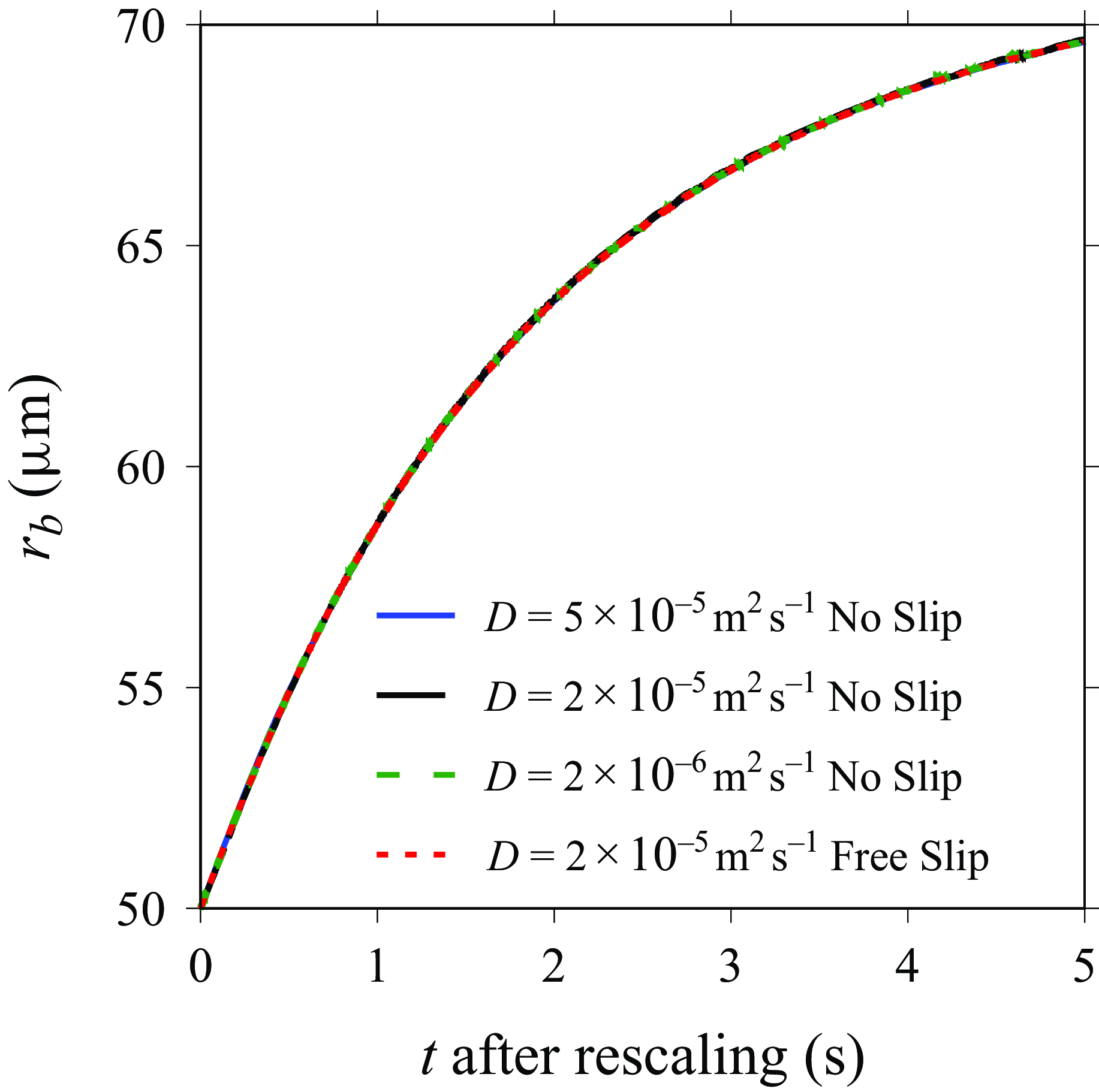
Figure 12. Influence of no-slip/free-slip condition at substrate, and manually enhancing the diffusion coefficient on the evolution of an unpinned bubble. The horizontal axis is the time after rescaling according to the ratio of the increased to the real diffusion coefficient. Here, $r_{b,{\textit{ini}}}=50 \, \unicode {x03BC}$
m.
$r_{b,{\textit{ini}}}=50 \, \unicode {x03BC}$
m. $r_{e}= 75 \, \unicode {x03BC}$
m,
$r_{e}= 75 \, \unicode {x03BC}$
m, $j=250$
A m
$j=250$
A m ${^-}^2$
,
${^-}^2$
, $\theta$
= 90°.
$\theta$
= 90°.
Appendix C. Influence of initial radius for unpinned bubbles
As can be seen in figure 13, unpinned bubbles of different initial radius start either to grow or to dissolve, but eventually are all approaching the same state of dynamic equilibrium. This gives numerical support to the theoretical stability condition (3.12) derived above. It also indicates that, in the cases considered here, convection is not important ( $Pe=r_b/D \,\boldsymbol\cdot\, {\rm d}r_b/{\rm d}t \ll 1$
), as otherwise the final bubble state could be influenced by the different impact of growth or shrinkage on the convective mass transfer.
$Pe=r_b/D \,\boldsymbol\cdot\, {\rm d}r_b/{\rm d}t \ll 1$
), as otherwise the final bubble state could be influenced by the different impact of growth or shrinkage on the convective mass transfer.
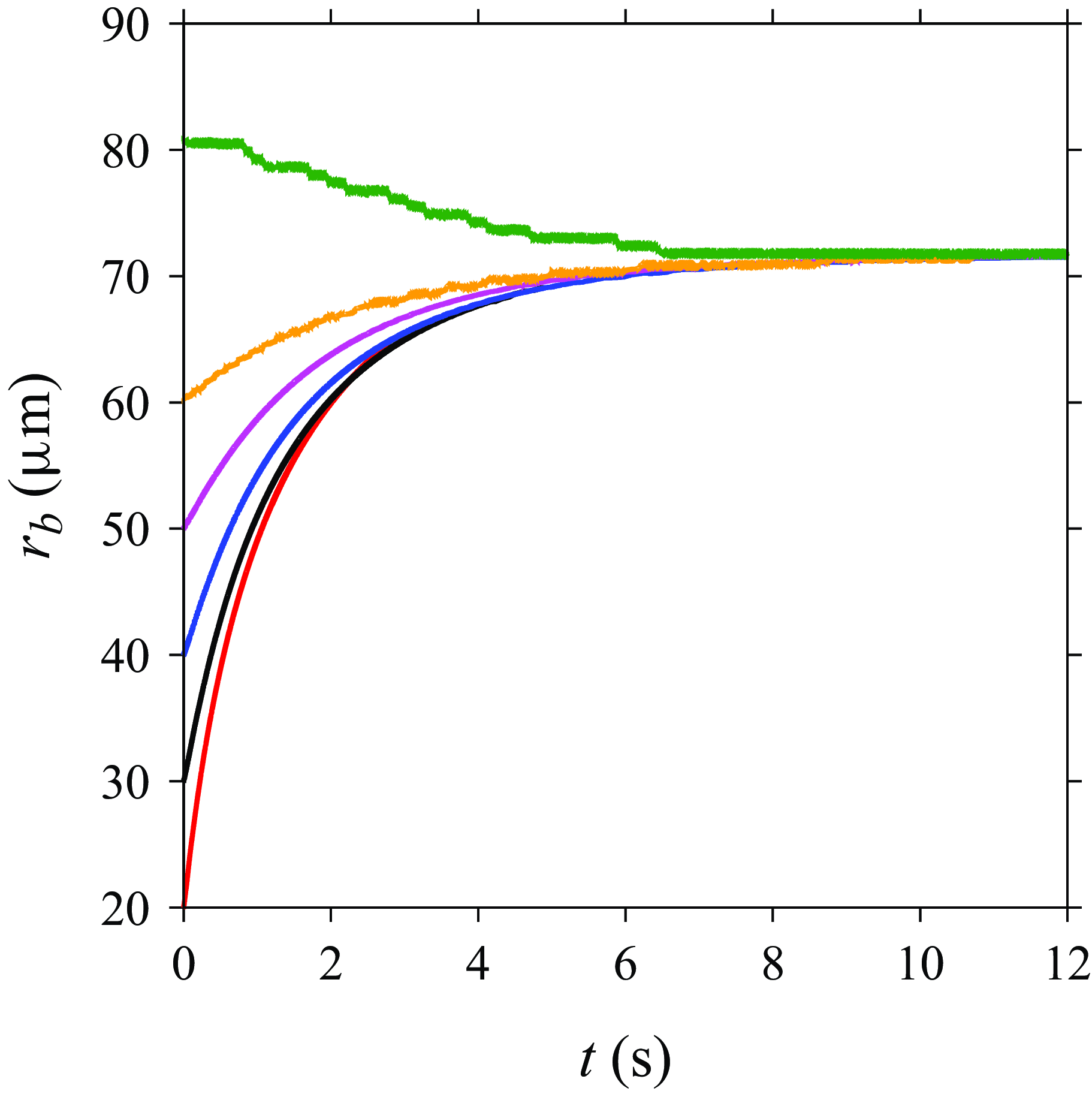
Figure 13. Temporal evolution of unpinned bubbles of different initial size $r_{b,{\textit{ini}}}$
ranging from 20 to 80
$r_{b,{\textit{ini}}}$
ranging from 20 to 80 $\unicode {x03BC}$
m and represented by different colours, where red, black, blue, magenta, orange and green represent
$\unicode {x03BC}$
m and represented by different colours, where red, black, blue, magenta, orange and green represent $r_{b,{\textit{ini}}}=20, \, 30, \, 40,\, 50,\, 60$
and 80
$r_{b,{\textit{ini}}}=20, \, 30, \, 40,\, 50,\, 60$
and 80 $\unicode {x03BC}$
m, respectively. All evolve towards the same dynamic equilibrium state. Here,
$\unicode {x03BC}$
m, respectively. All evolve towards the same dynamic equilibrium state. Here, $j=250$
A m
$j=250$
A m ${^-}^2$
,
${^-}^2$
, $r_e=75 \, \unicode {x03BC}$
m,
$r_e=75 \, \unicode {x03BC}$
m, $\theta =90$
°.
$\theta =90$
°.
Appendix D. Influence of bulk concentration
Here, we show theoretical results of the bubble end states obtained for zero over-saturation, i.e. $c_b=c_s$
and
$c_b=c_s$
and $\zeta =0$
. For the unpinned cases, figure 14, the current density becomes less important compared with the case of zero bulk concentration (
$\zeta =0$
. For the unpinned cases, figure 14, the current density becomes less important compared with the case of zero bulk concentration ( $\zeta =-1$
) shown in figure 6. The equilibrium bubble contact radius approaches the electrode radius in most situations. But for small
$\zeta =-1$
) shown in figure 6. The equilibrium bubble contact radius approaches the electrode radius in most situations. But for small $j$
and small
$j$
and small $r_e$
, a dissolution region also appears (white space). As in the case of
$r_e$
, a dissolution region also appears (white space). As in the case of $\zeta =-1$
, the critical electrode radius decreases with increasing
$\zeta =-1$
, the critical electrode radius decreases with increasing $j$
.
$j$
.
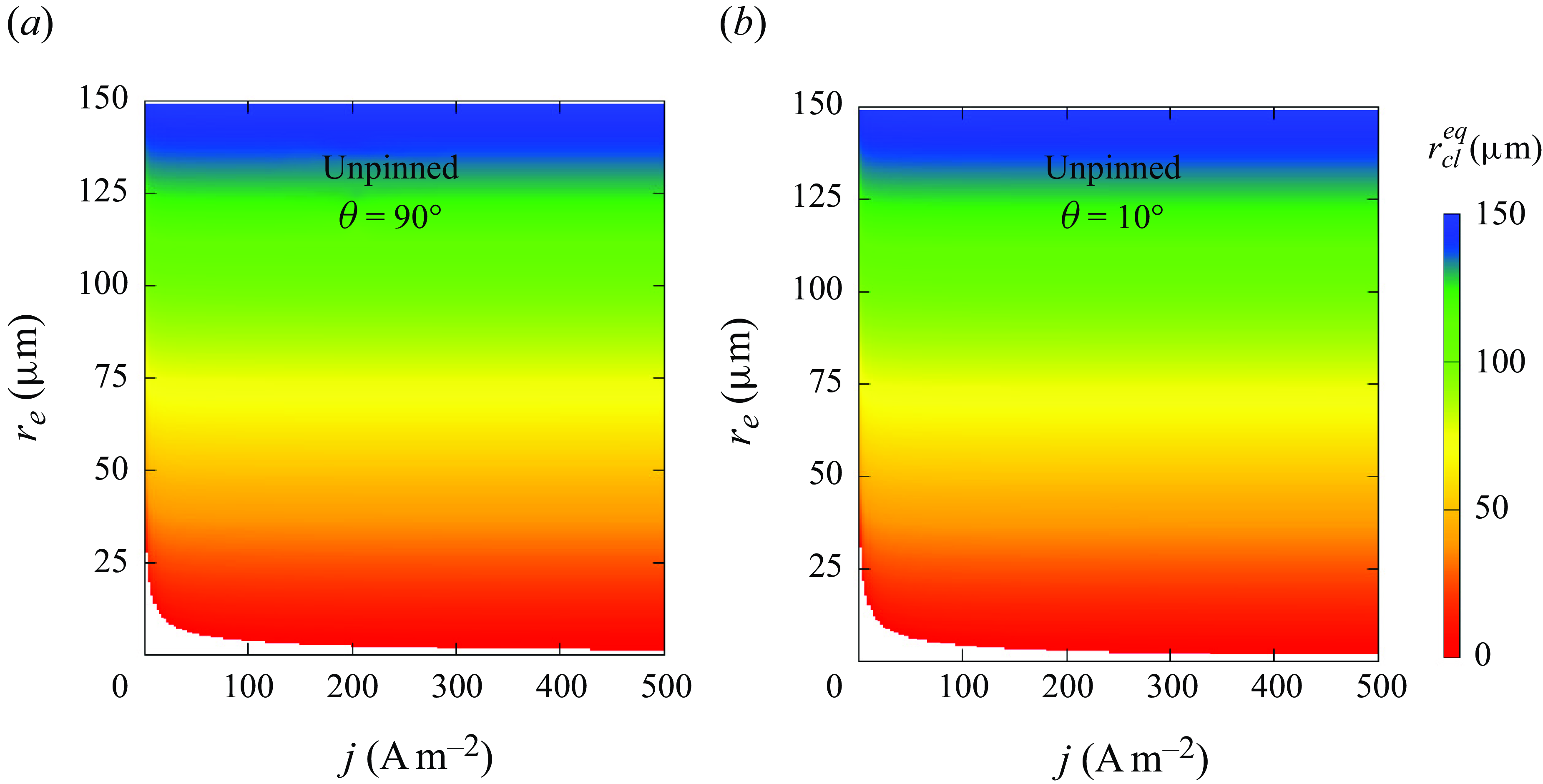
Figure 14. Theoretical solution of the equilibrium contact line radius $r_{cl,eq}$
(coloured surface) for unpinned bubbles versus electrode radius
$r_{cl,eq}$
(coloured surface) for unpinned bubbles versus electrode radius $r_e$
and applied current density
$r_e$
and applied current density $j$
when
$j$
when $c_b=c_s$
, i.e.
$c_b=c_s$
, i.e. $\zeta =0$
. Panels show (a)
$\zeta =0$
. Panels show (a) $\theta =90$
° and (b)
$\theta =90$
° and (b) $\theta =10$
°. The bottom white area marks complete dissolution.
$\theta =10$
°. The bottom white area marks complete dissolution.
For the pinned bubbles, figure 15, a dissolution region (white space below the coloured surface) and an unlimited growth region (grey space above the coloured surface) could be observed. The equilibrium contact angle decreases with increasing $r_e$
and
$r_e$
and $j$
. This is qualitatively also similar to the case of
$j$
. This is qualitatively also similar to the case of $\zeta =-1$
(figure 6), but the dissolution and growth regions have become smaller and larger, respectively, at the increased bulk concentration.
$\zeta =-1$
(figure 6), but the dissolution and growth regions have become smaller and larger, respectively, at the increased bulk concentration.
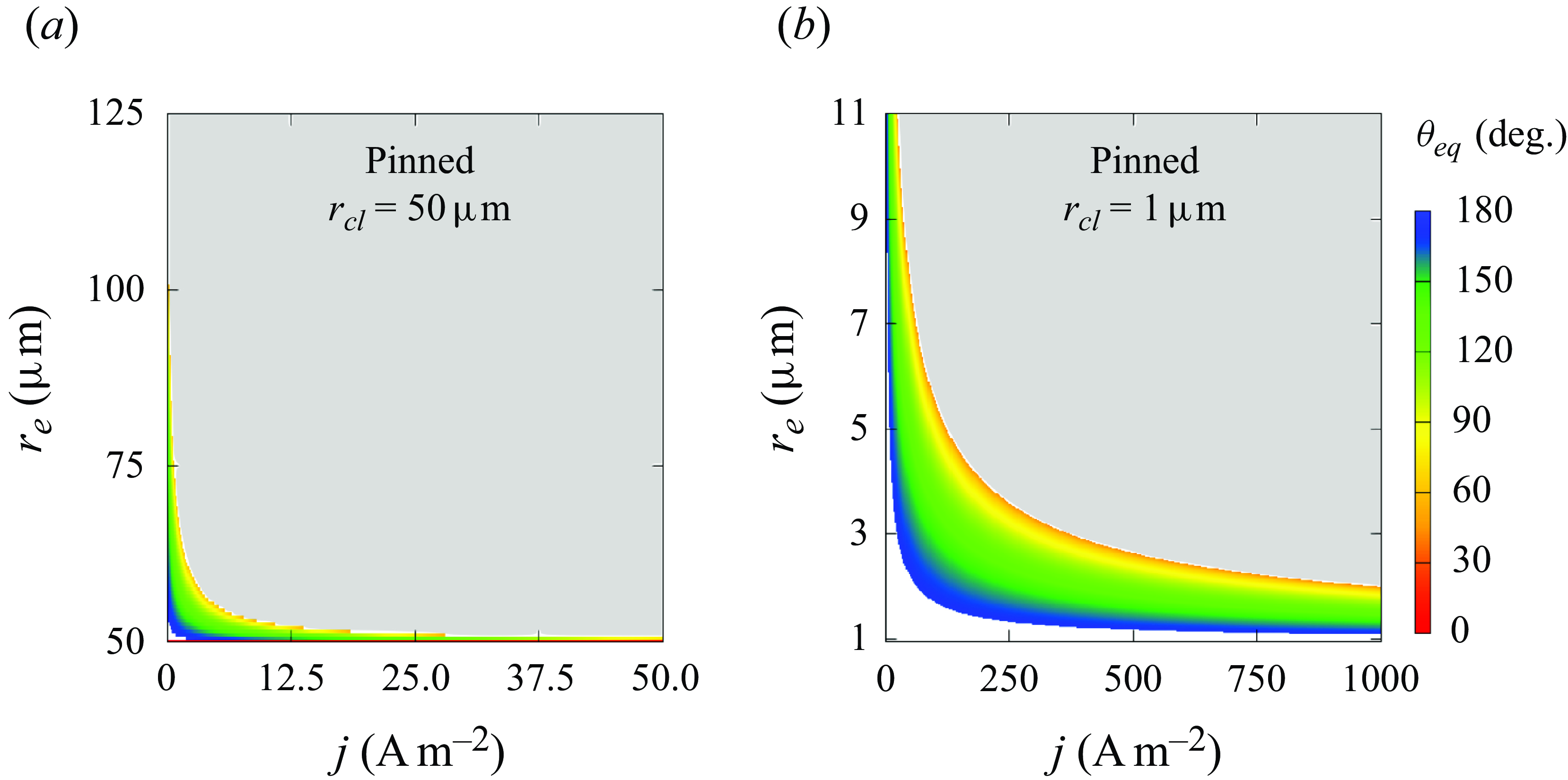
Figure 15. Theoretical solution of the equilibrium contact angle $\theta _{eq}$
(coloured surface) for pinned bubbles versus electrode radius
$\theta _{eq}$
(coloured surface) for pinned bubbles versus electrode radius $r_e$
and applied current density
$r_e$
and applied current density $j$
when
$j$
when $c_b=c_s$
, i.e.
$c_b=c_s$
, i.e. $\zeta =0$
. Panels show (a)
$\zeta =0$
. Panels show (a) $r_{\textit{cl}}=50 \, \unicode {x03BC}$
m and (b)
$r_{\textit{cl}}=50 \, \unicode {x03BC}$
m and (b) $r_{\textit{cl}}= 1 \, \unicode {x03BC}$
m. The grey top area represents unlimited growth. Note that, for the pinned bubbles in saturated liquid, there is theoretically no dissolution area. The white space at the bottom represents the region when
$r_{\textit{cl}}= 1 \, \unicode {x03BC}$
m. The grey top area represents unlimited growth. Note that, for the pinned bubbles in saturated liquid, there is theoretically no dissolution area. The white space at the bottom represents the region when $\theta _{eq}$
reaches 175°. At this point we stop the calculation and regard the bubble as having been reduced to a sufficiently flat surface to be considered as dissolved.
$\theta _{eq}$
reaches 175°. At this point we stop the calculation and regard the bubble as having been reduced to a sufficiently flat surface to be considered as dissolved.
Appendix E. Damköhler numbers
For the conditions considered in the simulations, the corresponding Damköhler numbers (Van Der Linde et al. Reference van der Linde, Moreno Soto, Peñas-López, Rodríguez-Rodríguez, Lohse, Gardeniers, van der Meer and Fernández Rivas2017) at equilibrium range from 0.04 to 30, but are mostly located between 0.1 and 1, as can be seen in figure 16.
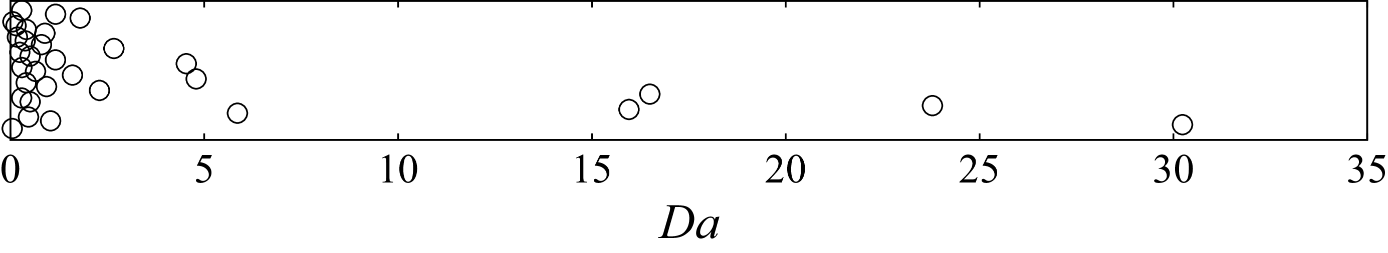
Figure 16. A summary of the Damköhler numbers of the stability states of the bubbles in the simulations. Each circle represents the result of one simulation.


 Open access