


1. Introduction
Particle transport in a fluid-driven fracture is a common and complex problem in the oil and gas industry. The particles transported in the hydraulic fracture can exhibit behaviours such as migration, settling and plugging (Dontsov & Peirce Reference Dontsov and Peirce2014). These behaviours, in turn, further influence the deformation and propagation of hydraulic fractures. In certain scenarios, such as the use of proppants in the early stage of hydraulic fracturing, particle plugging is undesirable since it can cause premature screen-out (Hosseini & Khoei Reference Hosseini and Khoei2020). Conversely, in other situations, such as temporary plugging and lost circulation control in drilling, effective plugging of the fracture is desired to limit and stop the fracture propagation (Mirabbasi et al. Reference Mirabbasi, Ameri, Alsaba, Karami and Zargarbashi2022; Zheng et al. Reference Zheng, Wang, Wang, Sun, Sun and Yu2024). Therefore, a comprehensive understanding of the plugging mechanism within a hydraulic fracture is essential for optimising the design of both hydraulic fracturing and well drilling operations.
Particle transport in hydraulic fractures is a fluid–solid coupling problem containing multiple physical processes, including solid deformation, slurry flow, particle transport and plugging, and fracture propagation and arrest. Numerical methods are an important approach to deal with such a complex problem (Cheng et al. Reference Cheng, Wu, Zhang, Huppert and Jeffrey2024b). The major challenges in a numerical approach lie in tracking the motion of particles and the interaction between particles, fluid and fracture. Existing numerical studies can be broadly categorised into three types. The first type considers fracture deformation and propagation. The particle transport is neglected, while the location, length and permeability of the plug are predefined. These simplifications allow for analytical modelling of the fracture by using linear elastic fracture mechanics (Morita & Fuh Reference Morita and Fuh2012; Shahri et al. Reference Shahri, Oar, Safari, Karimi and Mutlu2014; van Oort & Razavi Reference van Oort and Razavi2014; Feng & Gray Reference Feng and Gray2016). When coupling fracture deformation with fluid flow, various numerical models based on the finite element method (FEM) (Zhao et al. Reference Zhao, Santana, Feng and Gray2017) and the boundary element method (BEM) (Liu et al. Reference Liu, Ma, Chen, Wu, Zhang and Wu2020) have been developed. The second type focuses on modelling particle motions, while the fracture is treated as a stationary flow channel with a predefined fracture width. The majority of these numerical models solve the interaction between fluid flow and particle motion based on the Eulerian–Lagrangian framework, with examples provided by the coupling of computational fluid dynamics (CFD) and the discrete element method (DEM) (Li et al. Reference Li, Qiu, Zhong, Zhao and Huang2020; Wang et al. Reference Wang, Gong, Li and Yao2023; Pu et al. Reference Pu, Xu, Xu, Zhou, Li and Liu2023; Zhou et al. Reference Zhou, Yang, Xu, Song, Wang, Zheng, Zhou and Li2024). The third type of model considers both the fracture propagation and particle transport behaviours. The fracture deformation and propagation are simulated mainly by extended FEM or BEM, while the particle motion is modelled by DEM (Wang et al. Reference Wang, Li, Zhao and Zhang2020) or empirical constitutive model for suspension flow (Adachi et al. Reference Adachi, Siebrits, Peirce and Desroches2007; Dontsov & Peirce Reference Dontsov and Peirce2015; Hosseini & Khoei Reference Hosseini and Khoei2020; Wyatt & Huppert Reference Wyatt and Huppert2021; Zhang et al. Reference Zhang, Yang, Weng, Wang and Jeffrey2022a). Due to the coupling between particle transport, fluid flow and fracture deformation, the third type of numerical model is more representative of real-world conditions. This model is essential for investigating the plugging process within the fracture, and the fracture propagation behaviour when the plug forms.
The plugging location plays an important role in the fracture deformation and propagation behaviour. A series of experimental and numerical studies have been conducted on the formation location of the plug. The particle plugging can occur at the entry (Wang et al. Reference Wang, Zhou, Yang, Xu, Liu, Han, Wang, Ren and Liang2019a; Yang et al. Reference Yang, Feng, Li, Li, Li and Li2024), in the main channel (Yang et al. Reference Yang, Zhou, Feng, Tian, Yuan and Gao2019; Kang et al. Reference Kang, Zhou, Xu, Yang and You2023), and at the tip or leading edge of the fracture (Barree Reference Barree1991; Kumar, Kandasami & Sangwai Reference Kumar, Kandasami and Sangwai2024). Zhang et al. (Reference Zhang, Yu, Yang, Tian, Song, Sheng, Shi and Zhang2022b) developed a model for tip-plugging of a hydraulic fracture, and obtained the analytical solutions for the pressure decrement generated by the tip-plug. They argued that the effectiveness of the plugging can be measured by the pressure drop caused by the plug and the plug permeability. Wang et al. (Reference Wang, Wang, Cheng, Chen, Yang, Lv and Wang2022) experimentally investigated the entry-plugging process, and found that high flow rate and viscosity of the fluid can accelerate the diverter bridging process. Li et al. (Reference Li, Qiu, Zhong, Zhao and Huang2020) performed a numerical simulation of the fracture sealing process by using the CFD-DEM method. Their results indicated that the tip- or entry-plugging location can be distinguished by comparing the particle size and fracture width. The importance of the mechanical properties of fluid and geometric parameters of particles on the plugging location has been highlighted in these studies. Although the fracture width has been recognised as an important parameter on the transport and plugging behaviour of the particles, the fracture deformation and propagation are rarely considered by existing studies. This limitation may stem from constraints imposed by experimental conditions and numerical models. A few studies have developed comprehensive models to account for both fracture propagation and particle transport when investigating the plugging location (Luo et al. Reference Luo, Wong, Guo, Fu, Lu and Bunger2023; Yanqian et al. Reference Yanqian, Mengling, Kunchi and Feixu2023). Parameters such as rock elastic modulus, fracture toughness, fluid properties and particle size have been investigated in various models (Feng & Gray Reference Feng and Gray2016; Liu et al. Reference Liu, Ma, Chen, Wu, Zhang and Wu2020; Luo et al. Reference Luo, Wong, Guo, Fu, Lu and Bunger2023), and their independent effects on fracture deformation and particle transport have been widely studied. However, their coupling effect is rarely reported in the current studies. Since the dynamic plugging process involves multiple parameters associated with rock formation, fluid and particles, a general understanding of the fracture plugging requires a deeper exploration of the coupling effect of these parameters. How will the fracture behave before and after the plug forms? How to determine the location where particle plugging will occur within the fracture channel? What are the key parameters that control the fracture propagation and particle plugging behaviour? These are the important questions that have not been fully addressed by previous studies.
In this study, we aim to understand the dynamic plugging process of a hydraulic fracture driven by slurry flow. First, we present a numerical model accounting for fracture propagation, slurry flow and particle transport. This model combines a fully coupled hydraulic fracturing model that accounts for the fracture propagation and fluid flow, and a particle transport model based on an empirical constitutive model for suspension flow (Boyer, Guazzelli & Pouliquen Reference Boyer, Guazzelli and Pouliquen2011; Dontsov & Peirce Reference Dontsov and Peirce2014). To demonstrate the sealing effect of particle plugging on fracture propagation, we set a constant injection pressure, and predict the process where the fluid flowing into the fracture increases first and then decreases to zero. In order to extract the key parameters of the problem, a dimensional analysis is performed to reduce the number of controlling parameters to several dimensionless numbers. A series of numerical simulations are implemented in terms of the dimensionless numbers, and the evolution process of the fracture is investigated from particle entry to plugging occurrence.
This paper considers conditions that are more representative of those encountered in the drilling environment. During drilling, the drilling mud contains particles, such as clays added to the mud mix and rock particles generated by the drill bit, that are in suspension. Furthermore, the drilling mud is maintained at essentially a constant pressure. If a natural fracture is encountered at the exposed wellbore, then the drilling mud may enter, pressurise and extend along the natural fracture in a similar way to fluid entering a hydraulic fracture. Thus the assumptions used here of constant pressure at the fracture entry and a slurry maintaining that pressure are consistent with drilling mud loss into fractures. In contrast, most hydraulic fracturing operations for stimulation of reservoirs use a clean fluid pad to initiate and extend the fracture to some distance before a slurry carrying proppant is introduced.
The paper is organised as follows. In § 2, we formulate the problem for a hydraulic fracture driven by slurry flow, and provide the governing equations for solid deformation, slurry flow and particle transport. In § 3, a dimensional analysis is conducted to obtain the dimensionless forms of the equations and the dimensionless numbers. Section 4 introduces the numerical algorithms for solving the formulated problem. The numerical results for different stages of the fracture propagation and the different plugging modes are given in § 6. Finally, some discussions and conclusions are summarised in §§ 7 and 8.
2. Problem formulation
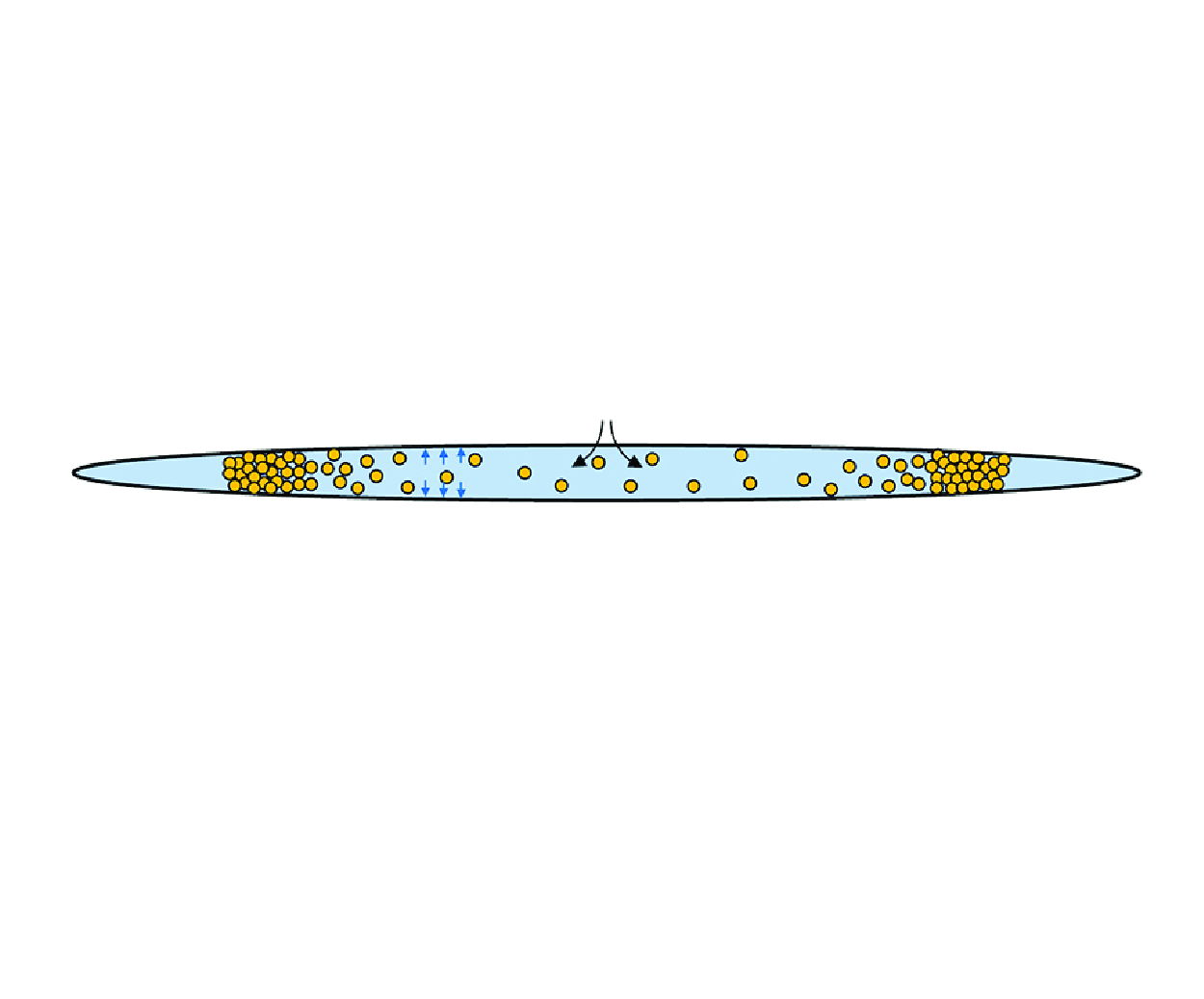
We consider a two-dimensional symmetric plane-strain fracture propagating in an impermeable linear elastic rock, as shown in figure 1. The rock formation is characterised by Young’s modulus E, Poisson’s ratio ν, and fracture toughness KIc . The fracture is driven by a constant wellbore pressure P w by injection of a mixture of incompressible Newtonian fluid and solid particles with a constant injected concentration ϕ 0, while the fluid pressure along the fracture p f , particle concentration ϕ, fracture width w, fracture length l, particle migration length l p , and fluid flux q are unknowns to be solved. Several assumptions are made to simplify the model.
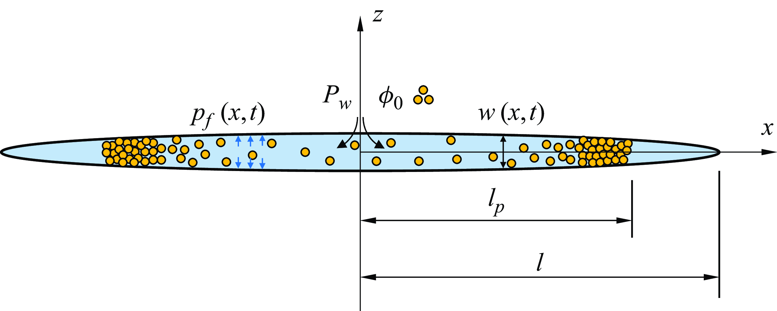
Figure 1. Symmetric plane-strain fracture driven by a mixture of fluid and solid particles.
-
i. The deformation of the wellbore is neglected. This assumption corresponds to a scenario where the fracture length is much larger than the wellbore radius, so that the wellbore becomes irrelevant on the scale of the fracture, reducing the model to a single fracture.
-
ii. The fracture propagation is modelled under the framework of linear elastic fracture mechanics, and the fracture propagation is considered to be quasi-static.
-
iii. The fluid flow in the fracture channel is laminar, and the fluid front coincides with the fracture front, i.e. the fluid lag is neglected.
-
iv. All injected solid particles are spherical and have the same radius. Since the fluid flow is one-dimensional, we do not consider the gravitational settling along the fracture height direction.
Before the wellbore pressurisation, the fracture with initial length l 0 is closed. As the fluid is injected, the fracture begins to open and propagate. When the fracture width becomes large enough compared to the particle size, the solid particles enter and are transported along the fracture. The particles can aggregate and consolidate at certain locations within the fracture channel during the particle migration, leading to the formation of plugs that block the fluid pressure from spreading along the fracture, and finally causing the fracture arrest. The aim of the proposed model is to quantitatively describe the dynamic plugging of a hydraulic fracture from its initiation to its arrest.
2.1. Solid deformation
Under the framework of linear elastic fracture mechanics, the tractions and displacements on fracture surfaces can be related by a pair of boundary integral equations (Hong & Chen Reference Hong and Chen1988; Portela, Aliabadi & Rooke Reference Portela, Aliabadi and Rooke1992)
 \begin{equation} \begin{array}{l} c_{ij}(x')\,u_{i}(x')+\displaystyle\int _{\Gamma }T_{ij}(x',x)\,u_{j}(x)\,\textrm{d}\Gamma =\displaystyle\int _{\Gamma }U_{ij}(x',x)\,t_{j}(x)\,\textrm{d}\Gamma, \\[3pt] \dfrac{1}{2}\sigma _{ij}(x')+\displaystyle\int _{\Gamma }S_{ijk}(x',x)\,u_{k}(x)\,\textrm{d}\Gamma =\displaystyle\int _{\Gamma }D_{ijk}(x',x)\,t_{k}(x)\,\textrm{d}\Gamma, \end{array} \end{equation}
where i, j and k denote Cartesian components, and i, j, k = 1, 2. Here, u
i
and σ
ij
are the displacement and stress components, respectively, t
j
is the traction component acting on the fracture surface, T
ij
and U
ij
are the Kelvin fundamental solutions for traction and displacement, respectively, S
ijk
and D
ijk
are linear combinations of derivatives of the Kelvin solutions, and $x'$
and x are the coordinates of the source point and field point on the boundary, respectively. Since we consider a straight fracture propagating along the x-axis as shown in figure 1, the point coordinates
$x'$
and x are the coordinates of the source point and field point on the boundary, respectively. Since we consider a straight fracture propagating along the x-axis as shown in figure 1, the point coordinates $x'$
and x are scalars rather than vectors in this paper. We have c
ij
=δ
ij
/2 for a smooth boundary at point
$x'$
and x are scalars rather than vectors in this paper. We have c
ij
=δ
ij
/2 for a smooth boundary at point $x'$
, and δ
ij
is the Dirac function. Due to the singularities exhibited by the fundamental solutions, the integrals in (2.1) should be interpreted as Cauchy principal-value integrals for strong singularity, and Hadamard principal-value integrals for hyper-singularity. Since we neglect the deformation of the wellbore, (2.1) can be reduced to one integral equation by using the properties of the fundamental solution (Portela et al. Reference Portela, Aliabadi and Rooke1992)
$x'$
, and δ
ij
is the Dirac function. Due to the singularities exhibited by the fundamental solutions, the integrals in (2.1) should be interpreted as Cauchy principal-value integrals for strong singularity, and Hadamard principal-value integrals for hyper-singularity. Since we neglect the deformation of the wellbore, (2.1) can be reduced to one integral equation by using the properties of the fundamental solution (Portela et al. Reference Portela, Aliabadi and Rooke1992)
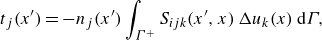 \begin{equation} t_{j}(x')=-n_{j}(x')\int _{{\Gamma ^{+}}}S_{ijk}(x',x)\,\Delta u_{k}(x)\,\textrm{d}\Gamma , \end{equation}
where Δu j is the discontinuous displacement component across the fracture surfaces, n j is the unit outward normal to the boundary, and Γ + represents one of the fracture surfaces. Equation (2.2) reduces the integral region from two fracture surfaces to only one fracture surface, which further reduces the computational cost (Cheng et al. Reference Cheng, Zhang, Chen and Wu2022a).
2.2. Slurry flow and particle transport
The slurry flow and particle transport are described by an empirical constitutive model for suspension flow in a fracture channel that is proposed by Dontsov & Peirce (Reference Dontsov and Peirce2014). Based on an experimental work unifying the rheology of suspension and granular matter (Boyer et al. Reference Boyer, Guazzelli and Pouliquen2011), this empirical model is capable of capturing the continuous transition between Poiseuille flow for small particle concentrations to Darcy’s law for maximum particle content. For both slurry flow and particle transport, the mass balance equation satisfies the equations
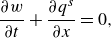 \begin{align} \frac{\partial w}{\partial t}+\frac{\partial q^{s}}{\partial x}=0,\end{align}
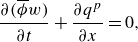 \begin{align} \frac{\partial (\overline{\phi }w)}{\partial t}+\frac{\partial q^{p}}{\partial x}=0,\end{align}
where w denotes the fracture width. Here, $\overline{\phi }$
= ϕ/ϕ
m
is the normalised particle concentration, where ϕ is the averaged particle volumetric concentration across the fracture width, and ϕ
m = 0.585 is the maximum allowed concentration for uniform spherical particles (Boyer et al. Reference Boyer, Guazzelli and Pouliquen2011). Once
$\overline{\phi }$
= ϕ/ϕ
m
is the normalised particle concentration, where ϕ is the averaged particle volumetric concentration across the fracture width, and ϕ
m = 0.585 is the maximum allowed concentration for uniform spherical particles (Boyer et al. Reference Boyer, Guazzelli and Pouliquen2011). Once $\overline{\phi }$
=1, i.e. ϕ = 0.585, it is considered that the plug is formed within the fracture (Majmudar et al. Reference Majmudar, Sperl, Luding and Behringer2007). Also, q
s
and q
p
are the fluxes for slurry and particle, respectively, and t and x denote time and coordinate along the fracture surface, respectively. According to Dontsov & Peirce (Reference Dontsov and Peirce2015), q
s
and q
p
are given by
$\overline{\phi }$
=1, i.e. ϕ = 0.585, it is considered that the plug is formed within the fracture (Majmudar et al. Reference Majmudar, Sperl, Luding and Behringer2007). Also, q
s
and q
p
are the fluxes for slurry and particle, respectively, and t and x denote time and coordinate along the fracture surface, respectively. According to Dontsov & Peirce (Reference Dontsov and Peirce2015), q
s
and q
p
are given by
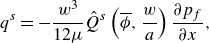 \begin{align} q^{s}=-\frac{w^{3}}{12\mu }\hat{Q}^{s}\left(\overline{\phi },\frac{w}{a}\right)\frac{\partial p_{f}}{\partial x},\end{align}
 \begin{align} q^{p}=B\hat{Q}^{p}\left(\overline{\phi },\frac{w}{a}\right)q^{s},\end{align}
where $\mu$
is the dynamic viscosity of clean fluid, p
f
is the fluid pressure, a is the particle radius, B is the blocking function introduced to determine the occurrence of particle bridging, which is given by (Dontsov & Peirce Reference Dontsov and Peirce2015)
$\mu$
is the dynamic viscosity of clean fluid, p
f
is the fluid pressure, a is the particle radius, B is the blocking function introduced to determine the occurrence of particle bridging, which is given by (Dontsov & Peirce Reference Dontsov and Peirce2015)
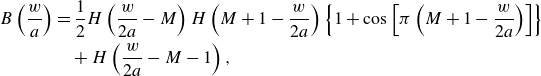 \begin{align} B\left(\frac{w}{a}\right)&=\frac{1}{2}H\left(\frac{w}{2a}-M\right)H\left(M+1-\frac{w}{2a}\right)\left\{1+\cos \left[\pi \left(M+1-\frac{w}{2a}\right)\right]\right\}\nonumber\\ &\quad{}+H\left(\frac{w}{2a}-M-1\right), \end{align}
with H the Heaviside step function, and M represents ‘several’ particle diameters, indicating that the particle bridging occurs when the fracture width is of the order of several particle diameters. We choose M = 3 in this paper to align with other numerical studies (Dontsov & Peirce Reference Dontsov and Peirce2015; Luo et al. Reference Luo, Wong, Guo, Fu, Lu and Bunger2023). The interaction between fluid and particle is characterised by two dimensionless functions, $\hat{Q}^{s}$
and
$\hat{Q}^{s}$
and $\hat{Q}^{p}$
, as shown in (2.5) and (2.6), which are given by
$\hat{Q}^{p}$
, as shown in (2.5) and (2.6), which are given by
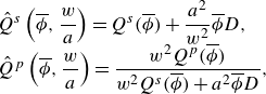 \begin{equation} \begin{array}{l} \hat{Q}^{s}\left(\overline{\phi },\dfrac{w}{a}\right)=Q^{s}(\overline{\phi })+\dfrac{a^{2}}{w^{2}}\overline{\phi }D,\\ \hat{Q}^{p}\left(\overline{\phi },\dfrac{w}{a}\right)=\dfrac{w^{2}Q^{p}(\overline{\phi })}{w^{2}Q^{s}(\overline{\phi })+a^{2}\overline{\phi }D}, \end{array} \end{equation}
where $D=8(1-\phi _{m})^{\overline{\alpha }}/(3\phi _{m})$
describes the permeability of the packed particles, and
$D=8(1-\phi _{m})^{\overline{\alpha }}/(3\phi _{m})$
describes the permeability of the packed particles, and $\overline{\alpha }=4.1$
(Dontsov & Peirce Reference Dontsov and Peirce2014). Here, Q
s
and Q
p
are univariate functions of
$\overline{\alpha }=4.1$
(Dontsov & Peirce Reference Dontsov and Peirce2014). Here, Q
s
and Q
p
are univariate functions of $\overline{\phi }$
, and their value can be found in the work of Dontsov & Peirce (Reference Dontsov and Peirce2014);
$\overline{\phi }$
, and their value can be found in the work of Dontsov & Peirce (Reference Dontsov and Peirce2014); $\hat{Q}^{s}$
describes the effect of particles on the slurry velocity, and
$\hat{Q}^{s}$
describes the effect of particles on the slurry velocity, and $\hat{Q}^{p}$
characterises the particle motion caused by slurry flow.
$\hat{Q}^{p}$
characterises the particle motion caused by slurry flow.
2.3. Boundary condition
Linear elastic fracture mechanics states that the fracture propagates when the stress intensity factor (SIF) exceeds the rock fracture toughness. At the tip of a hydraulic fracture under quasi-static propagation, we have
 \begin{equation} K_{{I}}=K_{{Ic}}, \end{equation}
where K I is the mode I SIF, and K Ic is the rock fracture toughness. The asymptotic expression for the fracture width near the tip is given by
 \begin{equation} w=4\sqrt{2/\pi }\,\frac{K_{{I}}}{E'}\left(l-\left| x\right| \right)^{1/2}\quad\left(\left| x\right| \rightarrow l\right), \end{equation}
where E ′ = E/(1-v 2) is the plane-strain elastic modulus. The fracture width, fluid flux and particle flux at the fracture tip are zero, given by
 \begin{equation} \left.w\right| _{x=\pm l}=0,\quad\left.q^{s}\right| _{x=\pm l}=0,\quad\left.q^{p}\right| _{x=\pm l}=0. \end{equation}
At the fracture inlet, the fluid pressure and injected particle concentration are both kept constant, namely
 \begin{equation} \left.p_{f}\right| _{x=0}=P_{w},\quad \left.q^{p}\right| _{x=0}=\left.q^{s}\right| _{x=0}\overline{\phi }_{0}, \end{equation}
where $\overline{\phi }_{0}$
= ϕ/ϕ
m is the normalised injected particle concentration.
$\overline{\phi }_{0}$
= ϕ/ϕ
m is the normalised injected particle concentration.
3. Dimensional analysis
To facilitate a comprehensive understanding of the model and reduce the computational cost, the following transformations are used:
 \begin{equation} \xi =\frac{x}{L^{*}},\quad \xi _{p}=\frac{l_{p}}{L^{*}},\quad {\Omega} =\frac{w}{W^{*}},\quad {\Pi} =\frac{p_{f}}{P^{*}},\quad \psi =\frac{q}{Q^{*}},\quad \tau =\frac{t}{T^{*}}, \end{equation}
where L *, W *, P *, Q * and T * are characteristic values of the fracture length, width, fluid pressure, flux and time, respectively. Also, l
p
is the distance between the particle migration front and fracture inlet, and ξ, ξ
p
, Ω, Π, ψ, $\tau$
are the dimensionless coordinate, particle migration distance, fracture width, fluid pressure, fluid flux and time, respectively. In order to keep the dimensionless equations uncluttered by numerical factors, the following material parameters are defined:
$\tau$
are the dimensionless coordinate, particle migration distance, fracture width, fluid pressure, fluid flux and time, respectively. In order to keep the dimensionless equations uncluttered by numerical factors, the following material parameters are defined:
 \begin{equation} \mu '=12\mu ,\quad E'=E/(1-v^{2}),\quad K'=4\sqrt{2/\pi }\,K_{{Ic}}. \end{equation}
For simplicity, $\mu$
′, E ′ and K ′ are referred to as the fluid viscosity, elastic modulus and toughness. The dimensionless governing equations are given by the following.
$\mu$
′, E ′ and K ′ are referred to as the fluid viscosity, elastic modulus and toughness. The dimensionless governing equations are given by the following.
-
Elasticity:
 \begin{equation} \Pi_{j}\left(\xi '\right)=-n_{j}(\xi ')\,{\mathcal{G}}_{e}\int _{{\Gamma ^{+}}}{\mathcal{S}}_{ijk}(\xi ',\xi )\,\Omega _{k}(\xi )\,{\textrm{d}}\it \Gamma (\xi ). \end{equation}
-
Mass continuity equations for slurry flow and particle transport:
 \begin{align} \frac{\dot{W}}{W}{\Omega} T^{*}+\dot{{\Omega} }T^{*}+{\mathcal{G}}_{f}\frac{\partial \psi ^{s}}{\partial \xi }=0,\end{align}
 \begin{align} \dot{\overline{\phi }}T^{*}{\Omega} +\frac{\dot{W}^{*}}{W^{*}}{\Omega} T^{*}\overline{\phi }+\dot{{\Omega} }T^{*}\overline{\phi }+\mathcal{G}_{f}\frac{\partial \psi ^{p}}{\partial \xi }=0.\end{align}
-
Fluxes for slurry and particle:
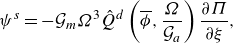 \begin{align} \psi ^{s}=-{\mathcal{G}}_{m}{\Omega} ^{3}\hat{Q}^{d}\left(\overline{\phi },\frac{{\Omega} }{{\mathcal{G}}_{a}}\right)\frac{\partial {\Pi} }{\partial \xi },\end{align}
 \begin{align} \psi ^{p}=B\hat{Q}^{p}\left(\overline{\phi },\frac{{\Omega} }{{\mathcal{G}}_{a}}\right)\psi ^{s}.\end{align}
-
Fracture propagation criterion:
 \begin{equation} {\Omega} ={\mathcal{G}}_{k}\left({\mathcal{G}}_{{\ell}}-\xi \right)^{1/2},\quad \xi \rightarrow {\mathcal{G}}_{\ell}. \end{equation}
-
Boundary conditions at the fracture inlet:
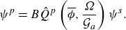
 \begin{equation} \left.{\mathcal{G}}_{p}{\Pi} \right| _{\xi =0}=1,\quad\left.{\mathcal{G}}_{\phi }\frac{\psi ^{s}}{\psi ^{p}}\right| _{\xi =0}=1. \end{equation}
-
Boundary conditions at the fracture tip:
 \begin{equation} \left.{\Omega} \right| _{\xi =\pm {{\mathcal{G}}_{\ell}}}=0,\quad\left.\psi ^{s}\right| _{\xi =\pm {{\mathcal{G}}_{\ell}}}=0,\quad\left.\psi ^{p}\right| _{\xi =\pm {{\mathcal{G}}_{\ell}}}=0. \end{equation}
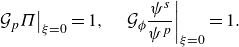
Eight dimensionless groups emerging from the dimensionless equations are defined as
 \begin{align} {\mathcal{G}}_{e}&=\frac{E'W^{*}}{P^{*}L^{*}},\quad {\mathcal{G}}_{f}=\frac{Q^{*}T^{*}}{W^{*}L^{*}},\quad {\mathcal{G}}_{m}=\frac{W^{*3}P^{*}}{\mu Q^{*}L^{*}},\quad {\mathcal{G}}_{k}=\frac{K_{Ic}L^{*1/2}}{E'W^{*}},\nonumber\\ &{\mathcal{G}}_{a}=\frac{a}{W^{*}},\quad {\mathcal{G}}_{\ell}=\frac{l}{L^{*}},\quad {\mathcal{G}}_{p}=\frac{P^{*}}{P_{w}},\quad {\mathcal{G}}_{\phi }=\overline{\phi}_{0}. \end{align}
The characteristic quantities will be obtained by imposing five constraints on these dimensionless groups. Note that the dimensionless unknowns ξ, Ω, Π and ψ should be of order 1 (Zhang, Jeffrey & Detournay Reference Zhang, Jeffrey and Detournay2005), and we set ${\mathcal{G}}_{e} , {\mathcal{G}}_{f} , {\mathcal{G}}_{\ell} , {\mathcal{G}}_{p} , {\mathcal{G}}_{m}$
to 1. Hence the following characteristic quantities are obtained:
${\mathcal{G}}_{e} , {\mathcal{G}}_{f} , {\mathcal{G}}_{\ell} , {\mathcal{G}}_{p} , {\mathcal{G}}_{m}$
to 1. Hence the following characteristic quantities are obtained:
 \begin{equation} L^{*}=l,\quad W^{*}=P_{w}l/E',\quad P^{*}=P_{w},\quad T^{*}=\mu 'E'^{2}/P_{w}^{3},\quad Q^{*}=P_{w}^{4}l^{2}/\left(E'^{3}\mu \right). \end{equation}
The remaining dimensionless groups, ${\mathcal{G}}_{k} , {\mathcal{G}}_{a} , {\mathcal{G}}_{\phi }$
, which are now renamed as
${\mathcal{G}}_{k} , {\mathcal{G}}_{a} , {\mathcal{G}}_{\phi }$
, which are now renamed as ${\mathcal{K}} , {\mathcal{A}}, \Phi$
, become
${\mathcal{K}} , {\mathcal{A}}, \Phi$
, become
 \begin{equation} {\mathcal{K}}=K'/\left(P_{w}l^{1/2}\right),\quad {\mathcal{A}}=E'a/\left(P_{w}l\right),\quad {\Phi} =\overline{\phi}_{0}. \end{equation}
The dimensionless numbers ${\mathcal{K}}$
and
${\mathcal{K}}$
and ${\mathcal{A}}$
can be interpreted as a dimensionless toughness and a dimensionless particle radius; Φ is simply the injected particle concentration. Since the fracture length is embedded in the dimensionless toughness and dimensionless particle radius, two length scales can be defined:
${\mathcal{A}}$
can be interpreted as a dimensionless toughness and a dimensionless particle radius; Φ is simply the injected particle concentration. Since the fracture length is embedded in the dimensionless toughness and dimensionless particle radius, two length scales can be defined:
 \begin{equation} L_{k}=K'^{2}/P_{w}^{2},\quad L_{a}=E'a/P_{w}. \end{equation}
Each length scale characterises a certain aspect of the physical process. When L
k $\gg$
l, i.e.
$\gg$
l, i.e. ${\mathcal{K}}\gg 1$
, the wellbore pressure is too small to propagate the fracture, and the fracture remains stationary. In contrast, when L
k
${\mathcal{K}}\gg 1$
, the wellbore pressure is too small to propagate the fracture, and the fracture remains stationary. In contrast, when L
k $\ll$
l, i.e.
$\ll$
l, i.e. ${\mathcal{K}}\ll 1$
, fracture propagation will occur. For the other length scale, when L
a
${\mathcal{K}}\ll 1$
, fracture propagation will occur. For the other length scale, when L
a $\gg$
l, i.e.
$\gg$
l, i.e. ${\mathcal{A}}\gg 1$
, the particle radius is much larger than the characteristic value of the fracture width, indicating that the particle cannot be transported in the fracture channel. In contrast, when L
a
${\mathcal{A}}\gg 1$
, the particle radius is much larger than the characteristic value of the fracture width, indicating that the particle cannot be transported in the fracture channel. In contrast, when L
a $\ll$
l, i.e.
$\ll$
l, i.e. ${\mathcal{A}}\ll 1$
, the particle is small enough compared to the characteristic fracture width, which means that the particles can transport freely in the fracture. Therefore, L
k
and L
a
measure the difficulty in fracture propagation and particle transport.
${\mathcal{A}}\ll 1$
, the particle is small enough compared to the characteristic fracture width, which means that the particles can transport freely in the fracture. Therefore, L
k
and L
a
measure the difficulty in fracture propagation and particle transport.
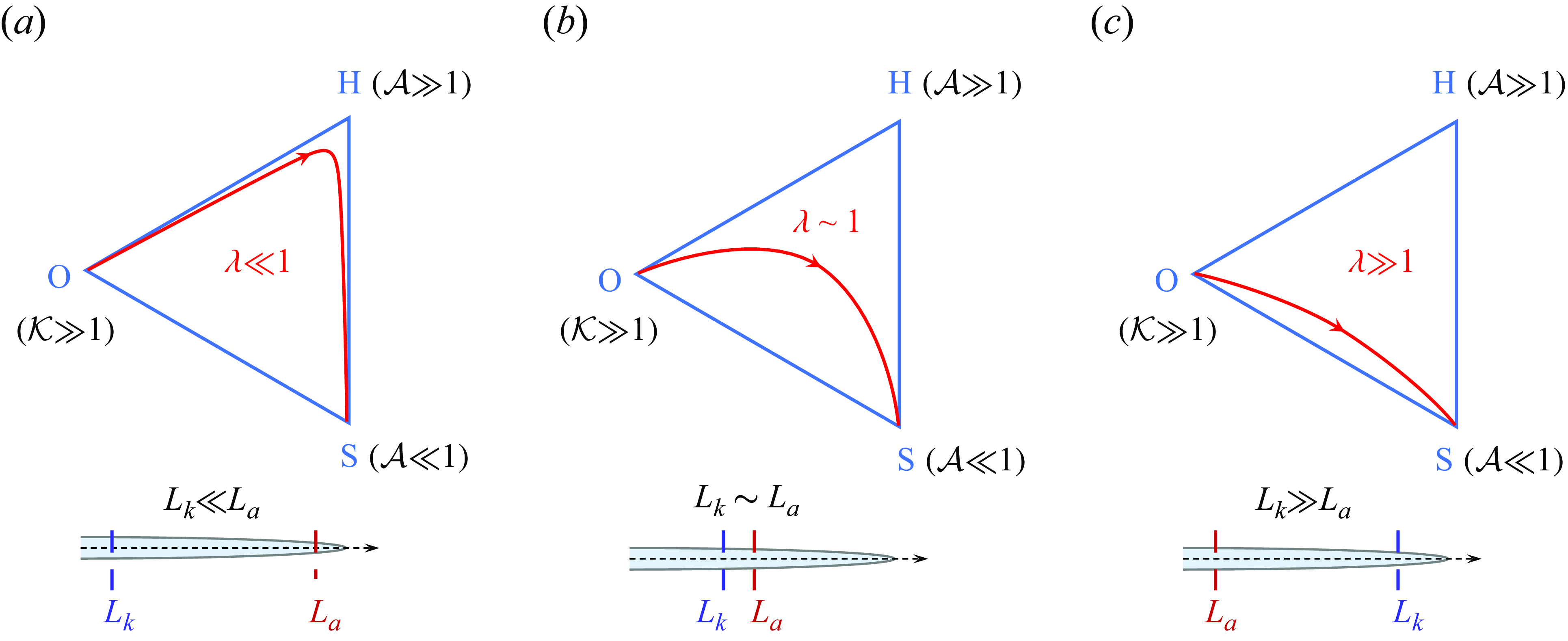
Figure 2. The transition between the limiting regimes in the parametric space.
As the sizes of L
k
and L
a
vary, there are three possible limiting regimes that can appear in the physical process. The first is the static regime where the fracture remains stationary when ${\mathcal{K}}\gg 1$
. The fracture propagation, fluid flow and particle transport will not happen in this condition, and the solution to this regime is independent of both
${\mathcal{K}}\gg 1$
. The fracture propagation, fluid flow and particle transport will not happen in this condition, and the solution to this regime is independent of both ${\mathcal{A}}$
and Φ. The second is the fluid-driven regime where the fracture propagation is driven by fluid while the particle is too large to enter or be transported in the fracture. This condition will happen when
${\mathcal{A}}$
and Φ. The second is the fluid-driven regime where the fracture propagation is driven by fluid while the particle is too large to enter or be transported in the fracture. This condition will happen when ${\mathcal{K}}\ll 1$
and
${\mathcal{K}}\ll 1$
and ${\mathcal{A}}\gg 1$
, corresponding to the case where fracture propagation will occur easily, while particle transport is difficult. The third is the slurry-driven regime where the particles begin to be transported in the fracture at the beginning of the fluid injection. This condition will happen when
${\mathcal{A}}\gg 1$
, corresponding to the case where fracture propagation will occur easily, while particle transport is difficult. The third is the slurry-driven regime where the particles begin to be transported in the fracture at the beginning of the fluid injection. This condition will happen when ${\mathcal{K}}\ll 1$
and
${\mathcal{K}}\ll 1$
and ${\mathcal{A}}\ll 1$
. For simplicity, the static regime, fluid-driven regime and slurry-driven regime are named as the O-regime, H-regime and S-regime, respectively. Once the fracture propagates,
${\mathcal{A}}\ll 1$
. For simplicity, the static regime, fluid-driven regime and slurry-driven regime are named as the O-regime, H-regime and S-regime, respectively. Once the fracture propagates, ${\mathcal{K}}$
and
${\mathcal{K}}$
and ${\mathcal{A}}$
will vary with the fracture length, leading to the transition between the limiting regimes, as shown in figure 2. The evolution of the fracture will go through the O-, H- and S-regimes one by one as the fracture length increases. When the initial fracture length exceeds L
k
, the fracture propagates and breaks away from the O-regime. Since the fracture width is small at the early stage of propagation, the particles are unable to enter the fracture yet, which corresponds to the H-regime. As the fracture width increases, the particles eventually enter and migrate inside the fracture, indicating the transition of fracture propagation into the S-regime. In specific situations, the fracture growth can be dominated by one of these regimes. If L
k
${\mathcal{A}}$
will vary with the fracture length, leading to the transition between the limiting regimes, as shown in figure 2. The evolution of the fracture will go through the O-, H- and S-regimes one by one as the fracture length increases. When the initial fracture length exceeds L
k
, the fracture propagates and breaks away from the O-regime. Since the fracture width is small at the early stage of propagation, the particles are unable to enter the fracture yet, which corresponds to the H-regime. As the fracture width increases, the particles eventually enter and migrate inside the fracture, indicating the transition of fracture propagation into the S-regime. In specific situations, the fracture growth can be dominated by one of these regimes. If L
k $\ll$
L
a
, then the fracture width will remain a small value compared to the particle size, indicating that the fracture will stay in the H-regime for a long period before the particle enters, as shown in figure 2(a). If L
k
$\ll$
L
a
, then the fracture width will remain a small value compared to the particle size, indicating that the fracture will stay in the H-regime for a long period before the particle enters, as shown in figure 2(a). If L
k $\gg$
L
a
, then the fracture width will be sufficient for particle transport as the fracture initiates, suggesting that the fracture will soon enter the S-regime while the H-regime is nearly bypassed, as shown in figure 2(c). Therefore, we find that the dominance of each regime can be characterised by the ratio of the two length scales, which is given by
$\gg$
L
a
, then the fracture width will be sufficient for particle transport as the fracture initiates, suggesting that the fracture will soon enter the S-regime while the H-regime is nearly bypassed, as shown in figure 2(c). Therefore, we find that the dominance of each regime can be characterised by the ratio of the two length scales, which is given by
 \begin{equation} \lambda =L_{k}/L_{a}={\mathcal{K}}^{2}/{\mathcal{A}}=K'^{2}/\left(P_{w}E'a\right). \end{equation}
This dimensionless number controls the evolution path of the fracture propagation in the parametric space spanned by the O-, H- and S-regimes.
4. Numerical algorithm
The numerical scheme used to solve the system of equations in § 2 consists of two parts. The first part is to solve the fluid–solid coupling problem between fracture deformation and slurry flow. The next part is to solve the particle distribution along the fracture channel. The general framework of the algorithm follows the one proposed by Dontsov & Peirce (Reference Dontsov and Peirce2015).
In the first part of the algorithm, an implicit scheme is used to solve the fracture deformation and fluid flow in a fully coupled way. For the solid deformation, the dual BEM is used to solve the integral equations in (2.1). The finite volume method is used to solve the equations governing the slurry flow. The fracture advances by the length of one element, and the time increment is iteratively determined by the implicit solver. If we denote the solution array in this part as X ={ w , l , p , q }, then the iterative scheme can be written as
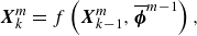 \begin{equation} \boldsymbol{X}_{k}^{m}=f\left(\boldsymbol{X}_{k-1}^{m},\overline{\boldsymbol{\phi }}^{m-1}\right), \end{equation}
where the subscript k is the iteration step, the superscript m represents the mth time step, and $\overline{\boldsymbol{\phi }}^{m-1}$
is the particle distribution in the previous time step. The details of the numerical discretisation and solution method can be found in our previous work (Cheng et al. Reference Cheng, Zhang, Zhang, Wu, Chen, Lei and Tan2022b, Reference Cheng, Wu, Zhang, Zhang, Han and Jeffrey2023, Reference Cheng, Wu, Wang, Chen, Zhao and Ma2024a).
$\overline{\boldsymbol{\phi }}^{m-1}$
is the particle distribution in the previous time step. The details of the numerical discretisation and solution method can be found in our previous work (Cheng et al. Reference Cheng, Zhang, Zhang, Wu, Chen, Lei and Tan2022b, Reference Cheng, Wu, Zhang, Zhang, Han and Jeffrey2023, Reference Cheng, Wu, Wang, Chen, Zhao and Ma2024a).
In the second part of the algorithm, the particle concentration is updated based on the solution of the first part. After the fracture propagation is solved, the particle concentration is solved by an explicit finite volume method. The major challenge in implementing the finite volume scheme lies in evaluating the particle flux between elements, especially when particle blocking occurs, because neglecting the propagation wave of the particles can lead to numerical inaccuracy in particle flux. Therefore, an upwind scheme is used to calculate the difference of the particle flux in (2.4), ensuring that the flux is calculated by using the values from upstream. The sign of the ‘wind’ (Dontsov & Peirce Reference Dontsov and Peirce2015; Wang, Elsworth & Denison Reference Wang, Elsworth and Denison2018) is given by
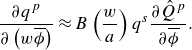 \begin{equation} \frac{\partial q^{p}}{\partial \left(w\overline{\phi }\right)}\approx B\left(\frac{w}{a}\right)q^{s}\frac{\partial \hat{Q}^{p}}{\partial \overline{\phi }}. \end{equation}
If the signs of two adjacent elements are the same, i.e. both positive or negative, then the difference of the particle flux can be calculated directly by the central difference scheme. If the signs are opposite, then the smaller flux of the two adjacent elements should be chosen in the calculation of the flux difference. Details of the explicit finite volume method and the upwind scheme can be found in Dontsov & Peirce (Reference Dontsov and Peirce2015).
Since an implicit scheme is employed in solving the nonlinear coupling between fracture deformation and slurry flow, the time step can be too large to fit into the explicit finite volume method when updating the particle concentration. In order to guarantee the stability of the explicit scheme, the time increment should be restricted by the Courant–Friedrichs–Lewy (CFL) condition (De Moura & Kubrusly Reference De Moura and Kubrusly2013). When the fracture propagation is solved at each step, the new time increment should be checked to see whether it satisfies the CFL condition. If the time increment is too large, then it will be split into several small time steps, with each sub-step meeting the CFL condition. Then the particle concentration is solved step by step.
5. Model validation
The present model will be validated in four aspects. First, the numerical solution of a fracture subjected to a uniform pressure distribution is validated against the analytical solution of a Griffith crack. This corresponds to the scenario of a fracture staying in the O-regime. Second, the numerical solution of a fluid-driven fracture is validated against the semi-analytical solution of a plane-strain hydraulic fracture under constant injection rate. Although the boundary condition in the H-regime is constant injection pressure, the effectiveness of the fluid–solid coupling algorithm can be validated. Third, the particle transport algorithm is validated by comparing it with the numerical solutions of a proppant transport problem. This corresponds to the scenario of a fracture staying in the S-regime. Finally, a mesh sensitivity analysis of the numerical simulator is conducted.
The analytical solution of a plane-strain fracture subjected to a uniform pressure is given by Sneddon & Elliot (Reference Sneddon and Elliot1946). The parameters used for validation are given in table 1: p 0 is the uniform pressure acting on the fracture surfaces, and L is the half-length of the fracture. Twenty boundary elements are used for the discretisation of the fracture surface, and the comparison of the fracture width profile between the numerical results and analytical solution is given in figure 3. It can be observed that the numerical results match well with the analytical results. The current model slightly overestimates the fracture width, with the maximum relative error occurring at the fracture tip, while most of the relative errors are below 1 %.
Table 1. Simulation parameters for the validation of a Griffith crack.
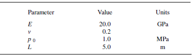
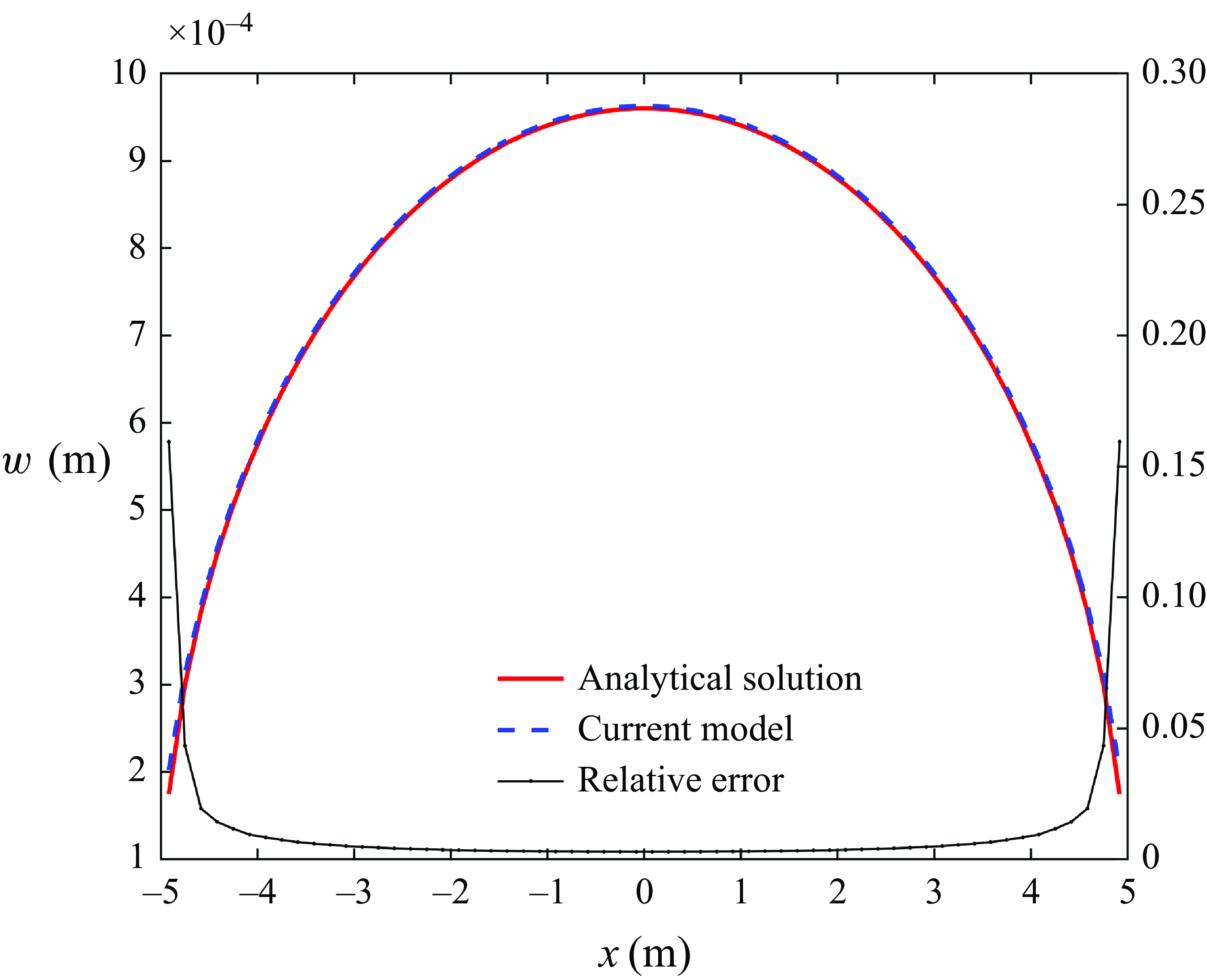
Figure 3. Comparison of the fracture width profile between current model and analytical solution.
The propagation of a plane-strain hydraulic fracture under constant injection rate exhibits self-similar characteristics. Here, we verify our fluid–solid couping algorithm with semi-analytical solution in a viscosity-dominated regime for a plane-strain hydraulic fracture (Adachi & Detournay Reference Adachi and Detournay2002). The simulation parameters are given in table 2. At the beginning of the simulation, the half-length of the fracture is set to be 0.5 m, and 10 boundary elements are used to discretise the initial fracture. Figure 4 shows the comparison of the injection pressure, fracture width at the fracture inlet, and fracture half-length between the numerical results and semi-analytical solutions. The relative error in figure 4 decreases rapidly with time, and the numerical predictions agree well with the semi-analytical solutions. Therefore, the fluid–solid couping algorithm is effective.
Table 2. Simulation parameters for a hydraulic fracture propagating in viscosity-dominated regime.
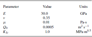
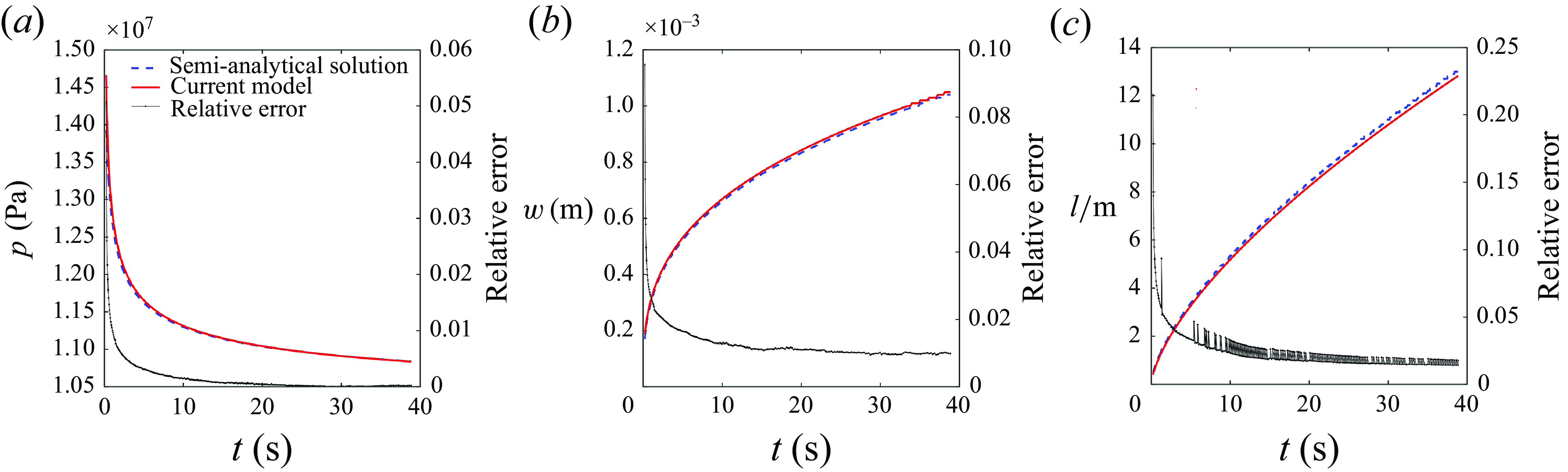
Figure 4. Comparison of (a) injection pressure, (b) fracture width at the fracture inlet and (c) fracture half-length.
The performance of the particle transport algorithm is crucial to the modelling of the fracture plugging process. Here, we apply the particle transport algorithm to the proppant transport in a vertical hydraulic fracture. The model set-up is consistent with an existing numerical study by Dontsov & Peirce (Reference Dontsov and Peirce2015). The initial fracture is set to be parallel to the direction of gravity, and its initial length is 1 m. A stress barrier is imposed 10 m away from the injection point, with magnitude 2.5 MPa. The fracture is driven by pure fluid with a constant injection rate for 1000 s, then the proppant is injected at a volume concentration ¯ϕ 0 = 0.2. The effect of gravitational settling is considered by adding a velocity term associated with gravity to (2.6) , which is given by
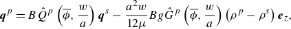 \begin{equation} \boldsymbol{q}^{p}=B\hat{Q}^{p}\left(\overline{\phi },\frac{w}{a}\right)\boldsymbol{q}^{s}-\frac{a^{2}w}{12\mu }Bg\hat{G}^{p}\left(\overline{\phi },\frac{w}{a}\right)\left(\rho ^{p}-\rho ^{s}\right)\boldsymbol{e}_{z}, \end{equation}
where g is the gravitational acceleration, ρ
p
and ρ
s
are densities of the particle and the fluid, respectively, and
e
z is the included angle cosine between the fracture and the vertical direction. The dimensionless function $\hat{G}^{p}$
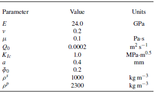
denotes the settling behaviour of the particles. The parameter settings are given in table 3.
$\hat{G}^{p}$
denotes the settling behaviour of the particles. The parameter settings are given in table 3.
Table 3. Simulation parameters for proppant transport in a vertical fracture.
The numerical results calculated by the current model are compared with the results of Dontsov & Peirce (Reference Dontsov and Peirce2015), and the profiles of particle concentration and fracture width in t = 1100, 3000 and 5000 s are shown in figure 5. We can find that gravity causes the particles on the negative axis to move faster than those on the positive axis. When t = 5000 s, a plug is formed in the lower part of the fracture near the tip region. Figure 5 shows good agreement between our model and existing numerical results, indicating that the particle transport and plugging behaviour can be captured properly by the current model.
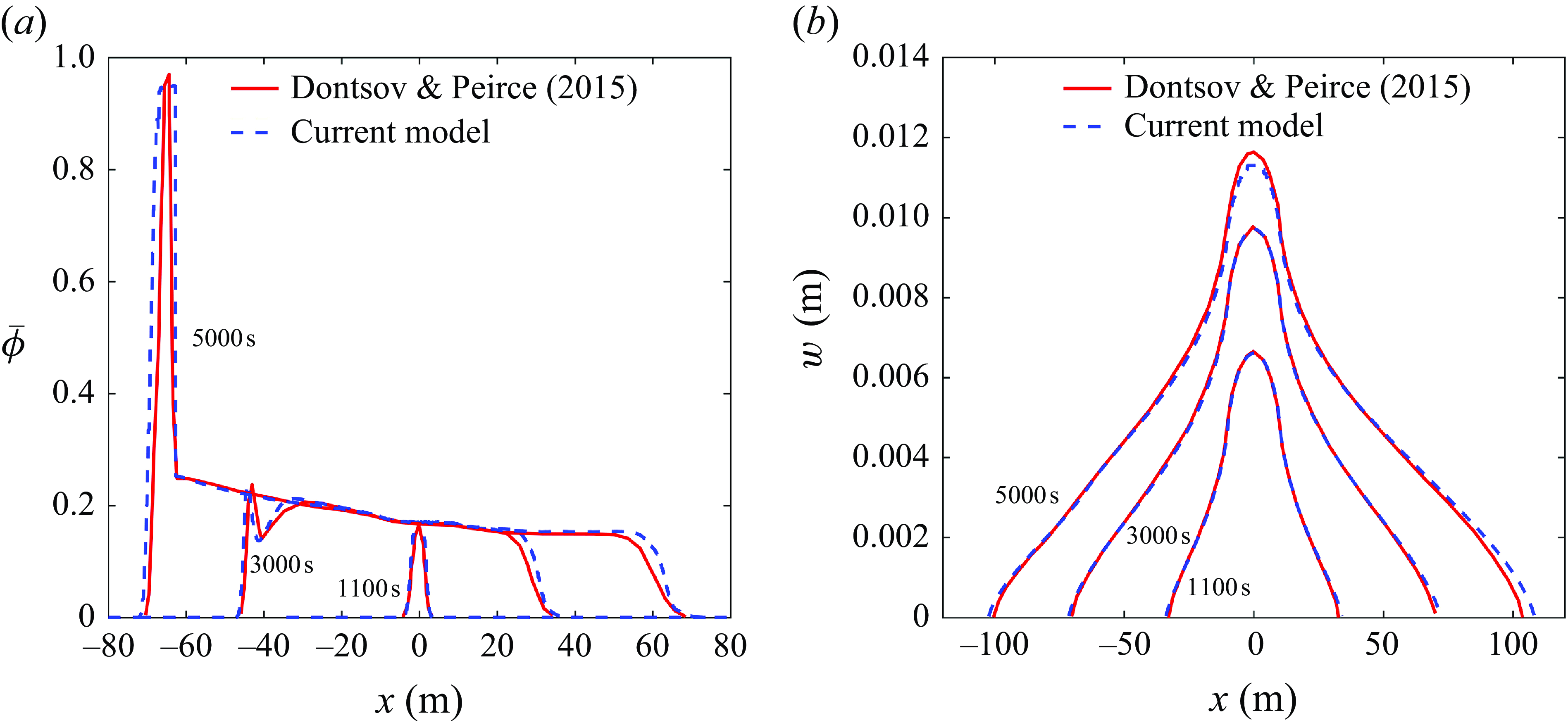
Figure 5. Comparison of the profiles of (a) particle concentration and (b) fracture width when t = 1100, 3000, and 5000 s.
A mesh sensitivity study is carried out to validate the convergence of the numerical model. Three simulation cases are performed, with element sizes set to 0.02, 0.01 and 0.005 m. The fracture length at the beginning of the simulation is set to 0.1 m. The injection pressure is P
w
= 2 MPa, and the particle size is a = 0.01 mm. Other parameters, such as the rock Young’s modulus E, Poisson’s ratio ν, fracture toughness K
Ic
, fluid viscosity $\mu$
, and injected particle concentration
$\mu$
, and injected particle concentration $\overline{\phi }_{0}$
, are consistent with table 3. Figure 6 presents the dependence of fracture width at the fracture inlet and particle concentration profile on element size. The variation in element size produces little difference in the evolution of fracture width and the distribution of particle concentration. This confirms the mesh independence of our numerical model.
$\overline{\phi }_{0}$
, are consistent with table 3. Figure 6 presents the dependence of fracture width at the fracture inlet and particle concentration profile on element size. The variation in element size produces little difference in the evolution of fracture width and the distribution of particle concentration. This confirms the mesh independence of our numerical model.
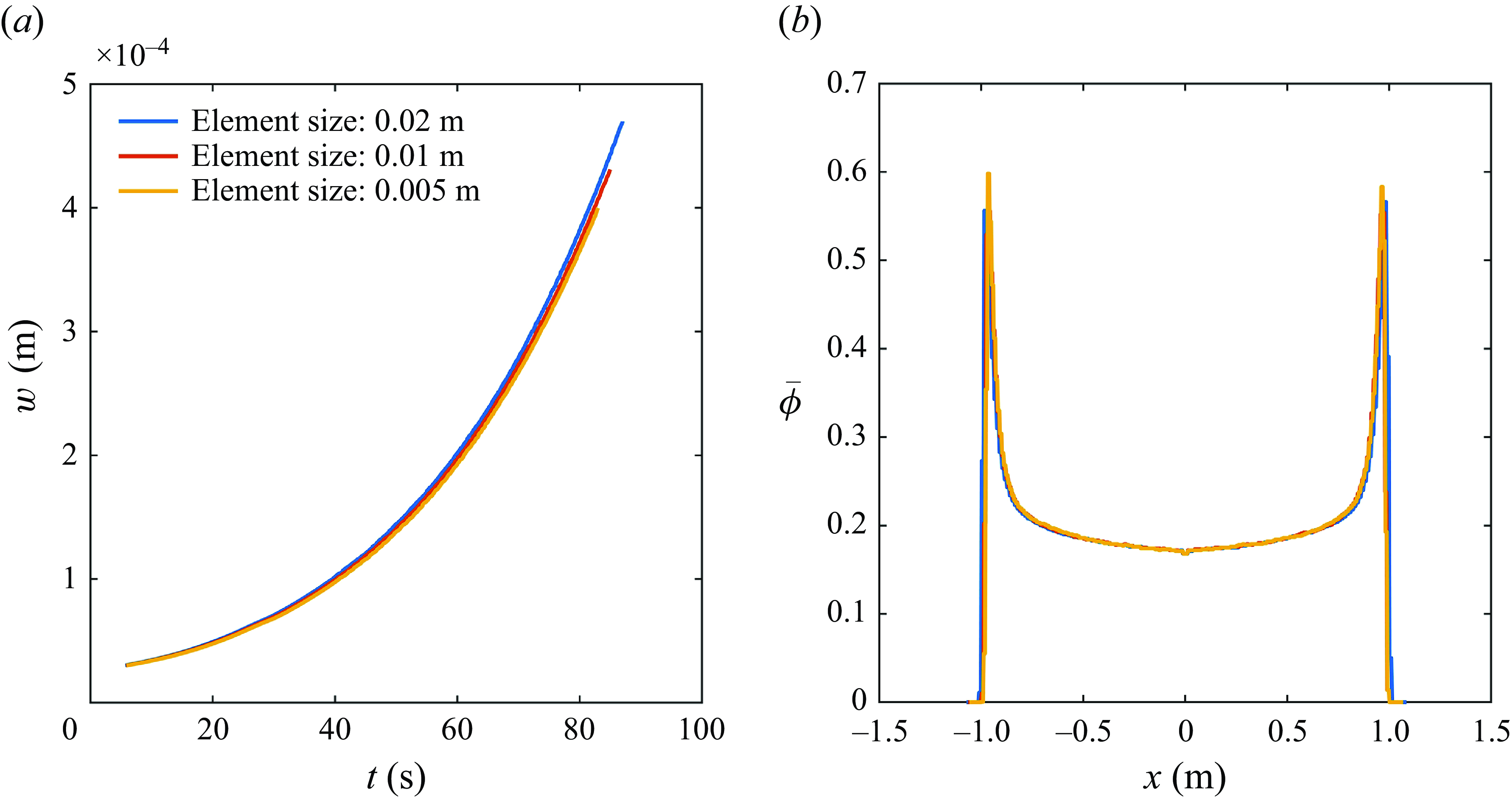
Figure 6. (a) Evolution of fracture width at the fracture inlet and (b) particle concentration profile at t = 70.1 s for different element sizes.
6. Numerical results
This section presents the numerical results of the evolution of a hydraulic fracture from its initiation to its arrest due to the plug formed by solid particles. First, the solutions of the limiting regimes are presented, and a comparison between the H-regime and S-regime is made to demonstrate the effect of the particle transport on fracture propagation. Then the role of λ on the transition between H- and S-regimes is shown in terms of a phase diagram determined by simulation results. Finally, two kinds of plugs and their influence on fracture propagation are presented.
6.1. Solutions of the limiting regimes and the transition between H- and S-regimes
In the O-regime, the fracture remains static and no fracture propagation occurs. In this case, the fracture will be fully and uniformly pressurised by wellbore pressure, which corresponds to the slow pressurisation of a hydraulic fracture (Lecampion, Abbas & Prioul Reference Lecampion, Abbas and Prioul2013). Therefore, the fracture width and SIF are given by (Rice Reference Rice1968)
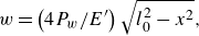 \begin{align} w=\left(4P_{w}/E'\right)\sqrt{l_{0}^{2}-x^{2}},\end{align}
 \begin{align} K_{I}=2\left(l_{0}/\pi \right)^{1/2}\int _{0}^{l_{0}}P_{w}\left(l_{0}^{2}-x^{2}\right)^{-1/2}\,\textrm {d}x=P_{w}\sqrt{\pi l_{0}},\end{align}
where l
0 is the initial half-length of the fracture. The fracture will propagate when l
0≥K
Ic
/(P
w
π 1/2), i.e. ${\mathcal{K}}\leq 4\sqrt{2}$
.
${\mathcal{K}}\leq 4\sqrt{2}$
.
When the SIF reaches the rock toughness, the fracture begins to propagate and enters the H-regime. The evolution of fracture width, fluid pressure and fluid flux of the hydraulic fracture in this regime is shown in figure 7. The simulation parameters are given in table 4. The fracture driven by constant inlet pressure grows rapidly, as shown in figure 7(a), and an exponential growth of the fluid flux is observed, as indicated by figure 7(c). This phenomenon is consistent with the theoretical studies of a gas-driven fracture under constant driving pressure (Nilson Reference Nilson1981, Reference Nilson1988). In engineering applications, the H-regime corresponds to the case where no plugging material is used, leading to the fluid loss to the fracture at an exponential rate.
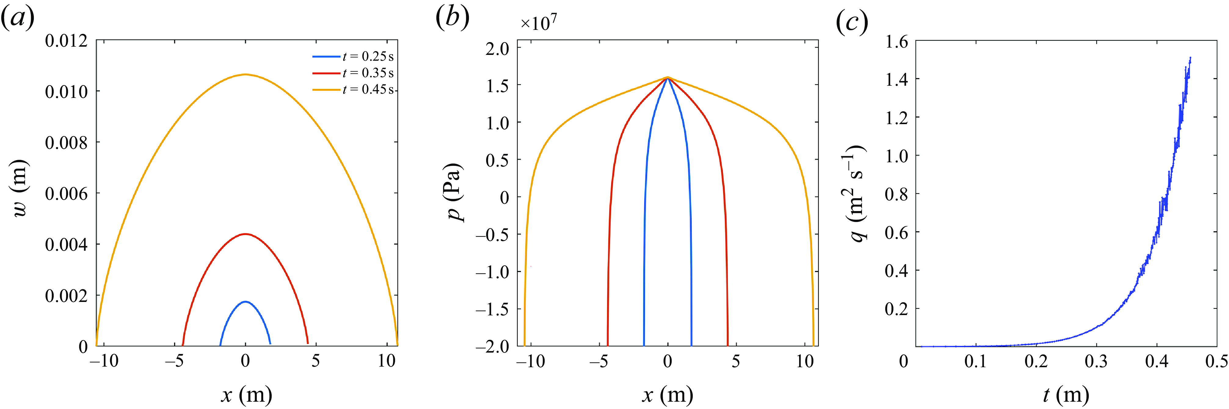
Figure 7. (a) The profiles of fracture width at 0.25, 0.35 and 0.45 s. (b) The profiles of fluid pressure at 0.25, 0.35 and 0.45 s. (c) The evolution of fluid flux in the H-regime.
Table 4. Simulation parameters for the H-regime.
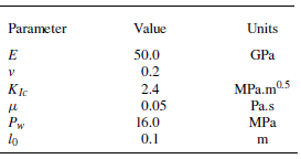
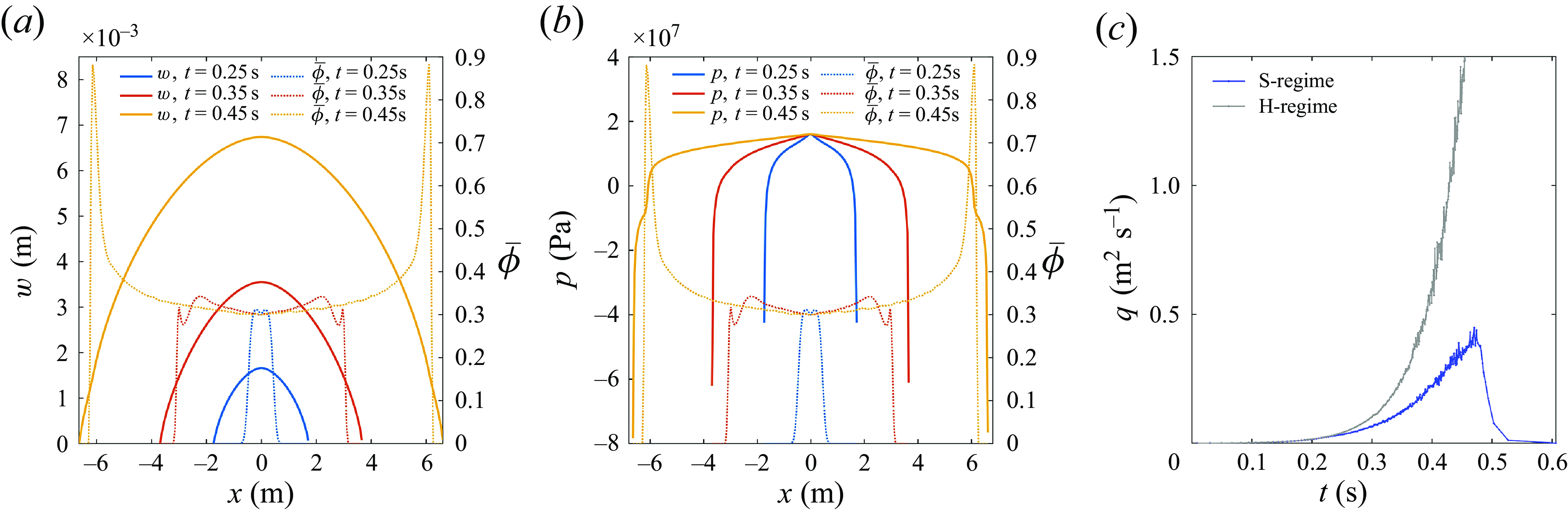
Figure 8. (a) The profiles of fracture width associated with particle concentration at 0.25, 0.35 and 0.45 s. (b) The profiles of fluid pressure associated with particle concentration at 0.25, 0.35 and 0.45 s. (c) The evolution of fluid flux in the S-regime.
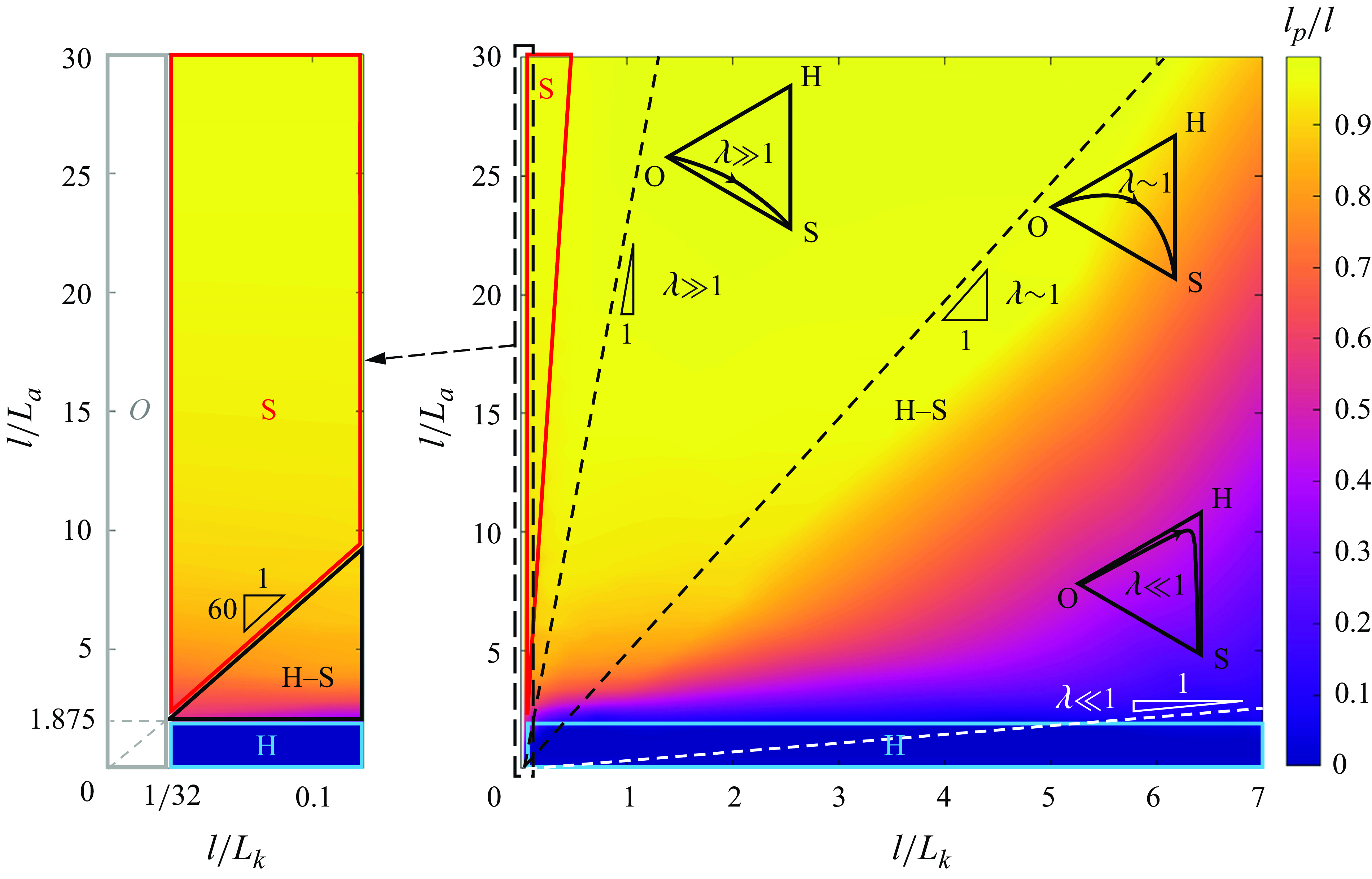
Figure 9. Evolution of the particle migration distance in the parametric space when $\overline{\phi }_{0}=0.2$
.
$\overline{\phi }_{0}=0.2$
.
If the particle size is small enough to transport in the fracture channel, then the fracture growth enters the S-regime. In the simulation, the particle radius is a = 0.4 mm, and the injected particle concentration is $\overline{\phi }_{0}$
= 0.3, with the other parameters the same as in table 4. The evolutions of particle concentration, fracture width, fluid pressure and fluid flux of the hydraulic fracture in this regime are shown in figure 8. The profile of the fracture width is similar to that of the H-regime as shown in figure 7, but the magnitude of the width is significantly reduced in the S-regime. The pressure profile in 0.25 s and 0.35 s is also similar to the H-regime. However, a rapid decrease of the fluid pressure at x = ±6 m can be observed in the S-regime. The pressure drop zone corresponds to the high particle concentration zone as shown in figure 8(b). This is because the particles have reached the near-tip region, where the fracture becomes narrow, so the particles begin to aggregate in this region and the concentration spikes, causing the slurry to become locally denser. Flow through a particle plug is difficult and is typically associated with a large pressure gradient through the plug. The pressure profile in 0.45 s exhibits the plugging process of the fracture where the particle aggregation blocks the fluid pressure from reaching the fracture tip. The existence of the particles and their aggregation behaviour increase the resistance in fluid flow, leading to a reduction in fluid flux compared to the H-regime, as shown in figure 8(c). As the pressure reduction in the near-tip region causes the SIF to become smaller than the rock toughness, the fracture arrests and fluid flux is reduced to zero. It can be noticed that the fluid flux experiences a rapid drop rather than decreasing gradually. Once the plug is formed, the fluid flow is blocked by the plug, making it difficult for the fluid pressure to reach the near-tip region. This causes the SIF to drop below the rock toughness. As the quasi-static fracture propagation no longer holds, the fracture arrests and the fluid can no longer enter the fracture, resulting in a rapid decrease of the fluid flux.
$\overline{\phi }_{0}$
= 0.3, with the other parameters the same as in table 4. The evolutions of particle concentration, fracture width, fluid pressure and fluid flux of the hydraulic fracture in this regime are shown in figure 8. The profile of the fracture width is similar to that of the H-regime as shown in figure 7, but the magnitude of the width is significantly reduced in the S-regime. The pressure profile in 0.25 s and 0.35 s is also similar to the H-regime. However, a rapid decrease of the fluid pressure at x = ±6 m can be observed in the S-regime. The pressure drop zone corresponds to the high particle concentration zone as shown in figure 8(b). This is because the particles have reached the near-tip region, where the fracture becomes narrow, so the particles begin to aggregate in this region and the concentration spikes, causing the slurry to become locally denser. Flow through a particle plug is difficult and is typically associated with a large pressure gradient through the plug. The pressure profile in 0.45 s exhibits the plugging process of the fracture where the particle aggregation blocks the fluid pressure from reaching the fracture tip. The existence of the particles and their aggregation behaviour increase the resistance in fluid flow, leading to a reduction in fluid flux compared to the H-regime, as shown in figure 8(c). As the pressure reduction in the near-tip region causes the SIF to become smaller than the rock toughness, the fracture arrests and fluid flux is reduced to zero. It can be noticed that the fluid flux experiences a rapid drop rather than decreasing gradually. Once the plug is formed, the fluid flow is blocked by the plug, making it difficult for the fluid pressure to reach the near-tip region. This causes the SIF to drop below the rock toughness. As the quasi-static fracture propagation no longer holds, the fracture arrests and the fluid can no longer enter the fracture, resulting in a rapid decrease of the fluid flux.
For most parameter settings, the hydraulic fracture will experience a transition from the H-regime to the S-regime instead of staying in one particular regime as the fracture length increases. The transition process is controlled by the ratio of two length scales λ, as indicated by dimensional analysis. Figure 9 shows the effect of λ on the evolution of particle migration distance when $\overline{\phi }_{0}$
= 0.2. Since
$\overline{\phi }_{0}$
= 0.2. Since $\lambda =L_{k}/L_{a}={\mathcal{K}}^{2}/{\mathcal{A}}$
, the propagation process of the fracture can be characterised by a straight line with slope λ, as shown in figure 9. We find that the O-, H- and S-regimes occupy a small fraction of the parametric space, as marked by the grey, blue and red wireframes, respectively. The O-regime is characterised by l/L
k
≤ 1/32 according to (6.2). The H-regime is described by l/L
a
≤ 1.875 and l/L
k
≥1/32, which is controlled by the blocking function in (2.7), indicating that the minimum fracture width required for the particle transport is 2Ma, where M is the number of particles for bridging, and a is the radius of one particle. The S-regime is possible only if the fracture can propagate while L
k
is sufficiently larger than L
a
. Hence this regime is characterised by λ≥60 and l/L
k
≥1/32, as indicated in figure 9. The rest of the region in the parametric space represents cases where the fracture will go through H- and S-regimes sequentially, which is denoted as the H–S regime. As indicated by the dimensionless analysis, the transition between H- and S-regimes is controlled by the magnitude of λ, which can be observed explicitly in the parametric space. For the small λ case, the fracture propagation will stay in the H-regime for a long time before the width is large enough for the particle transport, as shown by the white dashed line in figure 9. When λ increases, the fracture will soon go past the H-regime and enter the S-regime, as shown by the black dashed lines in figure 9. It can be observed from the contour that in the small λ case, the particles move slowly, and the particle migration length occupies only a small fraction of the fracture length. On the contrary, the particles move much faster in the large λ case, and the particle migration distance can soon reach over 90 % of the fracture length. This phenomenon demonstrates the effect of L
a
on particle transport, where a smaller L
a
is beneficial for particle transport in the fracture.
$\lambda =L_{k}/L_{a}={\mathcal{K}}^{2}/{\mathcal{A}}$
, the propagation process of the fracture can be characterised by a straight line with slope λ, as shown in figure 9. We find that the O-, H- and S-regimes occupy a small fraction of the parametric space, as marked by the grey, blue and red wireframes, respectively. The O-regime is characterised by l/L
k
≤ 1/32 according to (6.2). The H-regime is described by l/L
a
≤ 1.875 and l/L
k
≥1/32, which is controlled by the blocking function in (2.7), indicating that the minimum fracture width required for the particle transport is 2Ma, where M is the number of particles for bridging, and a is the radius of one particle. The S-regime is possible only if the fracture can propagate while L
k
is sufficiently larger than L
a
. Hence this regime is characterised by λ≥60 and l/L
k
≥1/32, as indicated in figure 9. The rest of the region in the parametric space represents cases where the fracture will go through H- and S-regimes sequentially, which is denoted as the H–S regime. As indicated by the dimensionless analysis, the transition between H- and S-regimes is controlled by the magnitude of λ, which can be observed explicitly in the parametric space. For the small λ case, the fracture propagation will stay in the H-regime for a long time before the width is large enough for the particle transport, as shown by the white dashed line in figure 9. When λ increases, the fracture will soon go past the H-regime and enter the S-regime, as shown by the black dashed lines in figure 9. It can be observed from the contour that in the small λ case, the particles move slowly, and the particle migration length occupies only a small fraction of the fracture length. On the contrary, the particles move much faster in the large λ case, and the particle migration distance can soon reach over 90 % of the fracture length. This phenomenon demonstrates the effect of L
a
on particle transport, where a smaller L
a
is beneficial for particle transport in the fracture.
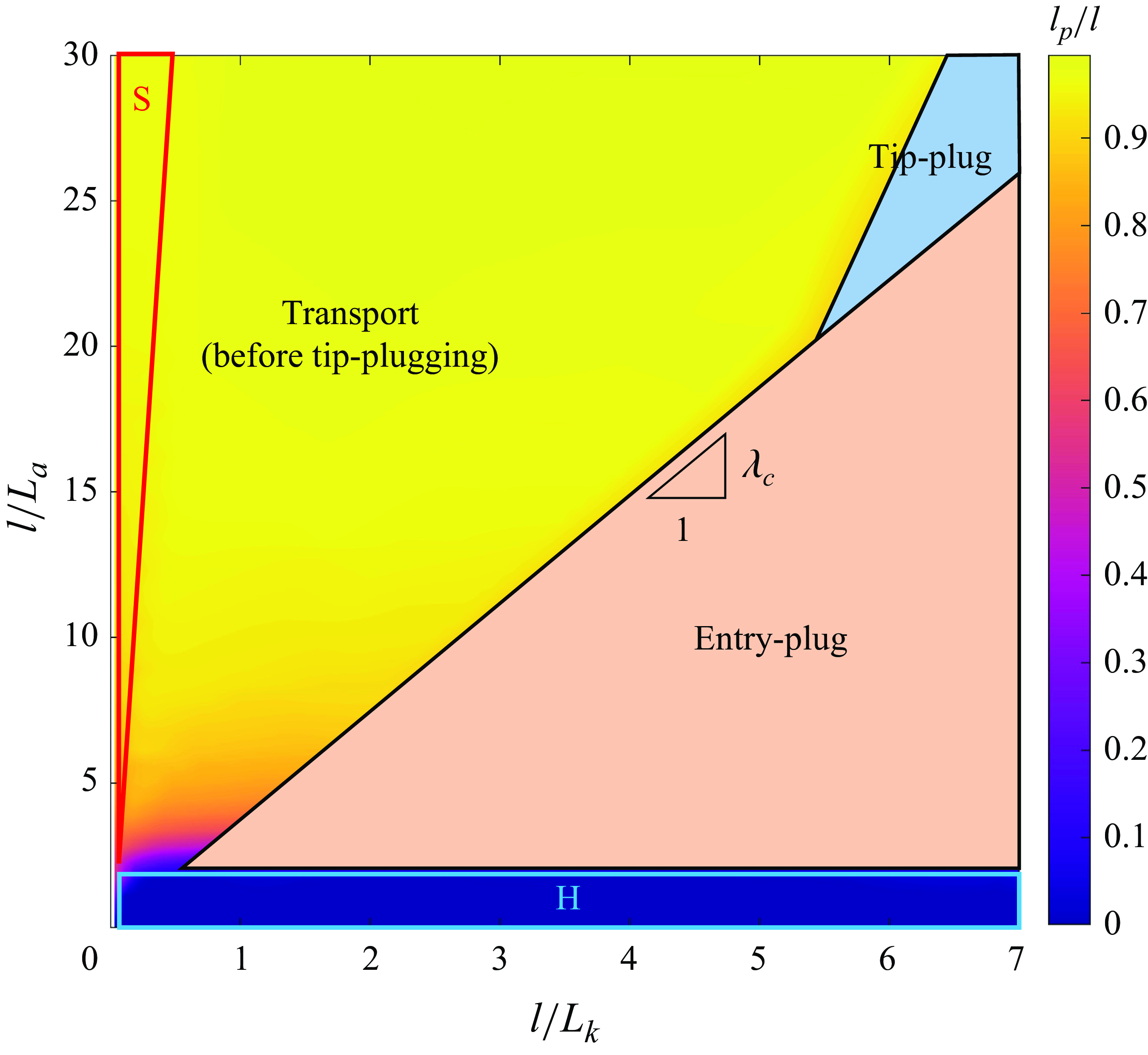
Figure 10. Distribution of entry- and tip-plugging in the parametric space when $\overline{\phi }_{0}=0.2$
.
$\overline{\phi }_{0}=0.2$
.
6.2. Tip- and entry-plugging of a hydraulic fracture
Two kinds of plug are observed from the numerical simulation. One is the tip-plug, where the plug forms near the fracture tip. The other is the entry-plug, where the plug forms near the fracture inlet. The numerical results indicate that the plugging location is influenced by λ as shown in figure 10. According to the state of the particles, the H–S regime can be further divided into three regions, where the tip- or entry-plug has occurred, and where the particles are still being transported prior to the formation of the tip-plug. The entry-plugging of the fracture occurs under small λ, which corresponds to scenarios with large particle size and small fracture toughness. When λ increases to a certain level, the particles start to be transported further instead of aggregating near the fracture entry. This is due to the fact that the fracture growth slows down when L k increases, and the velocity of particle transport also decreases as a result of decreased fluid flux, which hinders the quick build-up of particle concentration. When the particles transport to the near-tip region, where the fracture width becomes narrow, the particle concentration starts to build up, and eventually the tip-plug forms. The two kinds of plugging behaviour are divided by a boundary with a slope λ c . It should be noted that only the entry-plug and tip-plug are observed throughout the numerical results for different λ, while a continuous transition of plugging location from the entry-plug to somewhere between the fracture entry and tip region, and finally to the tip-plug, is not observed. This may be because the roughness of the fracture surface is not considered in our model. For a fracture with smooth surfaces, the numerical results imply a critical value of λ to distinguish the entry-plug and tip-plug, and λ c can be iteratively approximated by multiple simulations.
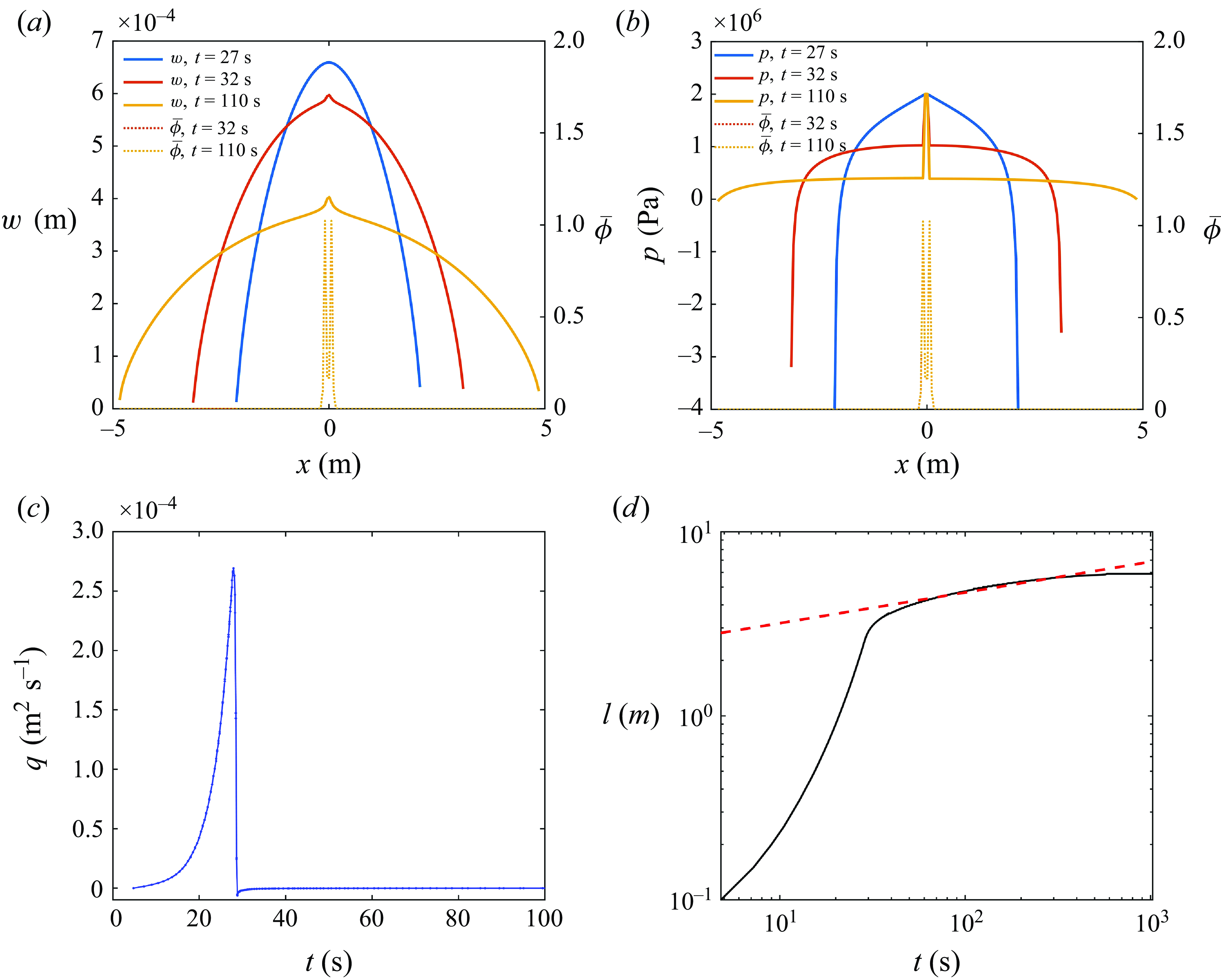
Figure 11. (a) The profiles of fracture width associated with particle concentration at 27, 32 and 110 s in the entry-plug case. (b) The profiles of fluid pressure associated with particle concentration at 27, 32 and 110 s in the entry-plug case. (c) The evolution of fluid flux and (d) the evolution of fracture half-length in the entry-plug case.
Since the plugging location differs between the entry-plug and tip-plug, the fracture propagation behaviour can also be different. Figure 8 is a typical example of the tip-plug occurring in the S-regime, and it can be observed that the particles form a high-concentration area near the fracture tip, which changes the pressure profile, as shown in figure 8(b). Figure 11 shows the fracture propagation behaviour when the entry-plug occurs, and the simulation parameters are listed in table 5. When t = 27 s, the fracture width is too small for the particle transport, so the fracture propagates in the H-regime. Once the width becomes large enough and the particles enter the fracture, the entry-plug quickly forms, and two peaks of particle concentration emerge near the fracture inlet in two wings of the fracture, as can be seen in figures 11(b,c) when t = 32 and 110 s. The entry-plug significantly changes the fluid pressure distribution compared to the H-regime, because the fluid pressure is decreased when the particles flow through the plug. Consequently, most of the fracture channel is loaded by low fluid pressure except for the fracture inlet, which leads to a smaller fracture width compared to the H-regime at t = 27 s, as shown in figure 11(a). We can infer from figure 11(c) that once the plug forms, the entry-plug almost blocks the fluid inflow entirely, which resembles the propagation of a hydraulic fracture after shut-in. In other words, the fracture is driven by fluid with constant volume after the entry-plug forms. One recalls the zero-toughness solution for a plane-strain fracture in the post-shut-in stage, where the power-law dependence between the fracture half-length and time is l∼t 1/6 (Liu Reference Liu2023; Liu & Lu Reference Liu and Lu2023). This power-law relation is observed in the evolution of the fracture length after the entry-plug occurs, as shown in figure 11(d).
Table 5. Simulation parameters for the entry-plug case.
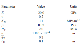
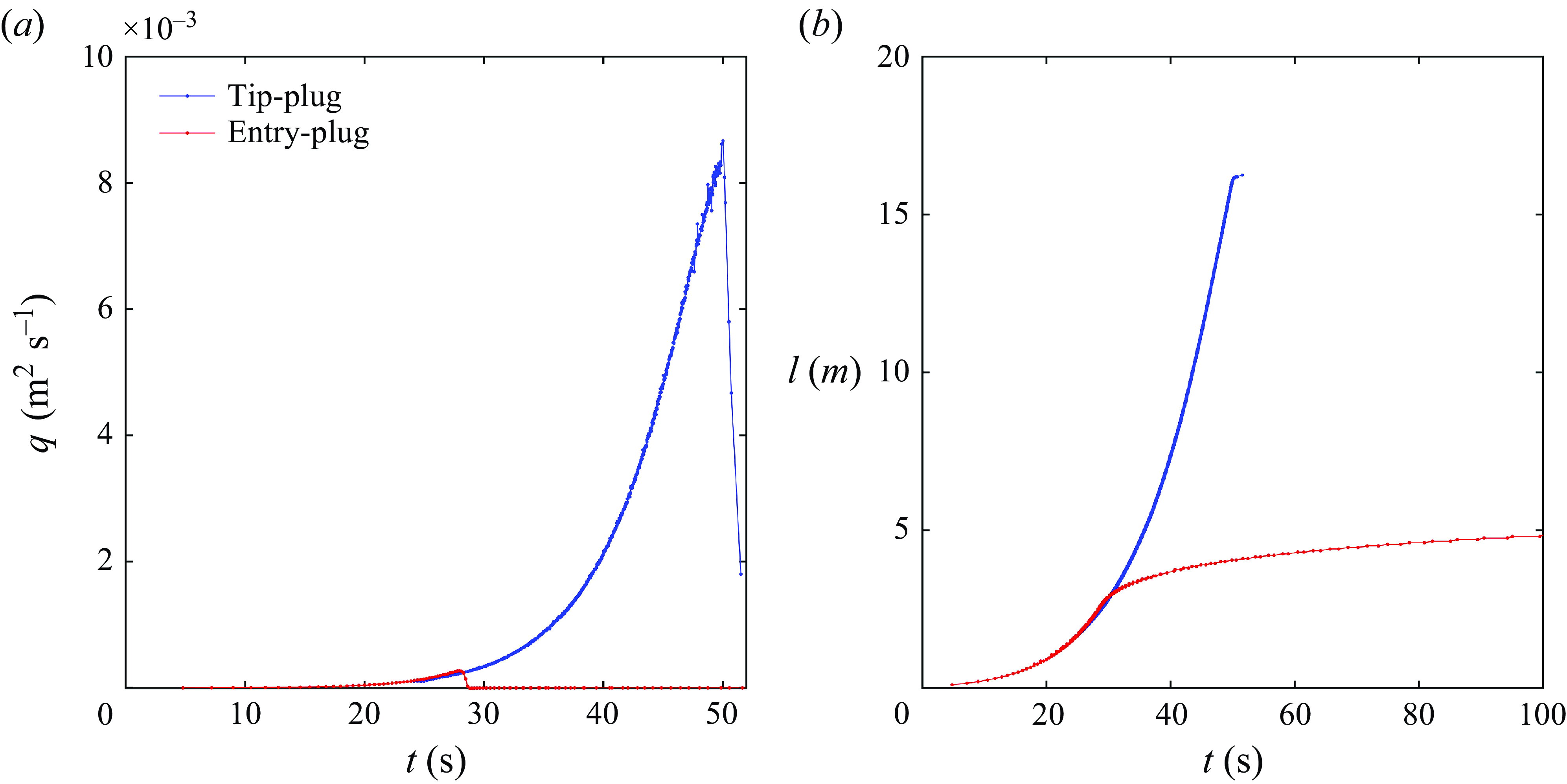
Figure 12. Evolution of (a) fluid flux and (b) fracture half-length when tip-plug and entry-plug occur.
A comparison between the effect of the tip-plug and entry-plug on the evolution of fluid inflow and fracture length is shown in figure 12. In order to generate the tip-plug, the particle radius is reduced to 7.39 × 10⁻⁵ m, while the other parameters are kept the same as in table 5. The tip-plug forms much later than the entry-plug, for two main reasons. Of course, leak-off from the fracture into the rock contributes to increasing the solid content of the slurry, making a plugging event more likely. The modelling done here, however, excludes leak-off by assuming an impermeable rock. Therefore, the first reason considered is that it takes more time for the particles to catch up with the advancing fracture tip than just move to somewhere near the fracture inlet. This allows the fracture to extend and widen, making plugging more difficult. It should be noted that the process of particles catching up with the fracture tip is related to the mechanism of shear-induced particle migration. The particles tend to avoid high shearing and move towards areas with lower shear rates. Consequently, the particles tend to concentrate in the central region of the flow channel, where the fluid velocity is higher compared to regions near the fracture wall. This means that the average particle velocity exceeds that of the fluid velocity, making it possible for the particles to catch up with the fracture tip even without the fluid leak-off. Second, the tip-plug only blocks the fluid pressure from reaching the fracture tip, while a large portion of the fluid is still pressurised by high fluid pressure. Therefore, the fracture propagation will not stop easily until the particle concentration is high enough to seal the fracture. On the contrary, once the entry-plug forms, the fluid pressure is significantly reduced when the fluid infiltrates through the plug region, restricting the high-pressure zone to a small region around the fracture inlet. Therefore, the fluid volume in the fracture is much smaller in the entry-plug case than in the tip-plug case. Due to rapid increase in the fluid flux before the fracture is plugged, the fracture length is longer in the tip-plug case than in the entry-plug case. In engineering applications, such as wellbore strengthening and temporary plugging, it is often desired to plug the fracture as quickly as possible and minimise the volume of fluid leaking into the fracture. In these cases, entry-plugging is the preferred way to seal the hydraulic fracture, compared to tip-plugging.
6.3. Transition between tip- and entry-plugging
The previous two subsections discuss mainly the effect of λ on the transition among the limiting regimes and plugging location. According to dimensional analysis, there is another dimensionless parameter that has not been discussed: the injected particle concentration $\overline{\phi }_{0}$
. Numerical results show that
$\overline{\phi }_{0}$
. Numerical results show that $\overline{\phi }_{0}$
exerts a significant impact on the plugging location. Figure 13 shows the distribution of entry- and tip-plugging in the parametric space when
$\overline{\phi }_{0}$
exerts a significant impact on the plugging location. Figure 13 shows the distribution of entry- and tip-plugging in the parametric space when $\overline{\phi }_{0}$
varies. The results indicate that the entry-plugging occupies a larger portion of the parametric space as the injected particle concentration increases, and the critical slope λ
c
that characterises the boundary between entry- and tip-plugging also increases with
$\overline{\phi }_{0}$
varies. The results indicate that the entry-plugging occupies a larger portion of the parametric space as the injected particle concentration increases, and the critical slope λ
c
that characterises the boundary between entry- and tip-plugging also increases with $\overline{\phi }_{0}$
. When
$\overline{\phi }_{0}$
. When $\overline{\phi }_{0}$
reaches 0.6, the entry-plug case covers the whole H–S regime. In other words, for a fracture propagating in the H–S regime, particle plugging can occur only near the fracture entry. Since
$\overline{\phi }_{0}$
reaches 0.6, the entry-plug case covers the whole H–S regime. In other words, for a fracture propagating in the H–S regime, particle plugging can occur only near the fracture entry. Since $\overline{\phi }_{0}$
is not included in the blocking function, it is evident that
$\overline{\phi }_{0}$
is not included in the blocking function, it is evident that $\overline{\phi }_{0}$
does not influence the transition between the O-, H- and S-regimes. With a given value of
$\overline{\phi }_{0}$
does not influence the transition between the O-, H- and S-regimes. With a given value of $\overline{\phi }_{0}$
, the evolution of the fracture is controlled by λ, as shown in the phase diagram in figure 2. The effect of
$\overline{\phi }_{0}$
, the evolution of the fracture is controlled by λ, as shown in the phase diagram in figure 2. The effect of $\overline{\phi }_{0}$
on the fracture propagation can be regarded as introducing an additional axis to the previous two-dimensional phase diagram, as shown in figure 13(e). Every cross-section of the phase diagram contains information about the evolution path of the fracture and the plugging location of the particles under a given value of
$\overline{\phi }_{0}$
on the fracture propagation can be regarded as introducing an additional axis to the previous two-dimensional phase diagram, as shown in figure 13(e). Every cross-section of the phase diagram contains information about the evolution path of the fracture and the plugging location of the particles under a given value of $\overline{\phi }_{0}$
. This three-dimensional phase diagram demonstrates the joint effect of λ and
$\overline{\phi }_{0}$
. This three-dimensional phase diagram demonstrates the joint effect of λ and $\overline{\phi }_{0}$
on the dynamic plugging of a propagating hydraulic fracture.
$\overline{\phi }_{0}$
on the dynamic plugging of a propagating hydraulic fracture.
Figure 13. Distribution of entry- and tip-plugging in the parametric space when (a) $\overline{\phi }_{0}$
= 0.1, (b)
$\overline{\phi }_{0}$
= 0.1, (b) $\overline{\phi }_{0}$
= 0.2, (c)
$\overline{\phi }_{0}$
= 0.2, (c) $\overline{\phi }_{0}$
= 0.4 and (d)
$\overline{\phi }_{0}$
= 0.4 and (d) $\overline{\phi }_{0}$
= 0.6. (e) The role of
$\overline{\phi }_{0}$
= 0.6. (e) The role of $\overline{\phi }_{0}$
in the parametric space.
$\overline{\phi }_{0}$
in the parametric space.
Since λ
c
characterises the boundary distinguishing the entry- and tip-plugging, it can be used as an indicator to predict the plugging location once the dependence of $\overline{\phi }_{0}$
on λ
c
is determined. The quantitative relation between
$\overline{\phi }_{0}$
on λ
c
is determined. The quantitative relation between $\overline{\phi }_{0}$
and λ
c
can be obtained by approximating λ
c
through multiple numerical simulations for each given
$\overline{\phi }_{0}$
and λ
c
can be obtained by approximating λ
c
through multiple numerical simulations for each given $\overline{\phi }_{0}$
, as shown in figure 14. It can be noted that λ
c
increases monotonically with
$\overline{\phi }_{0}$
, as shown in figure 14. It can be noted that λ
c
increases monotonically with $\overline{\phi }_{0}$
, and λ
c
keeps increasing after it reaches 60, indicating that the entry-plugging begins to occur in the S-regime. Figure 14 provides an efficient approach to predict the plugging location in a hydraulic fracture. If a data point (
$\overline{\phi }_{0}$
, and λ
c
keeps increasing after it reaches 60, indicating that the entry-plugging begins to occur in the S-regime. Figure 14 provides an efficient approach to predict the plugging location in a hydraulic fracture. If a data point ( $\overline{\phi }_{0}$
, λ) is above the
$\overline{\phi }_{0}$
, λ) is above the $\overline{\phi }_{0}$
–λ
c
curve, then a tip-plug will occur in the fracture. Conversely, if the point (
$\overline{\phi }_{0}$
–λ
c
curve, then a tip-plug will occur in the fracture. Conversely, if the point ( $\overline{\phi }_{0}$
, λ) is below the curve, then an entry-plug will be formed.
$\overline{\phi }_{0}$
, λ) is below the curve, then an entry-plug will be formed.
Figure 14. Relation between $\overline{\phi }_{0}$
and λ
c
.
$\overline{\phi }_{0}$
and λ
c
.
7. Discussion
Since the present model neglects the effect of fluid leak-off on the fracture propagation, the present model is applicable for reservoirs with low permeability. Since all the fluid is stored in the fracture when there is no fluid leak-off, the fluid pressure builds up quickly instead of dissipating due to fluid loss to the formation. Consequently, the fracture width increases faster than that in the leak-off case, which makes plug formation more difficult. Therefore, this paper provides a conservative prediction of the fracture plugging process.
Fluid leak-off can impose significant effect on the propagation of the fracture. First, it can introduce an additional propagation regime into the model. When the fluid leak-off plays a dominated role in the fracture propagation process, most of the fluid injected at the fracture inlet infiltrates into the surrounding medium, which means that the fracture volume tends to zero (Bunger, Detournay & Garagash Reference Bunger, Detournay and Garagash2005; Adachi & Detournay Reference Adachi and Detournay2008). In this case, the particles cannot enter the fracture like the O- and H-regime, while the fluid is leaking from the wellbore into the rock through the fracture. In addition to the new propagation regime, the fluid leak-off will have a significant impact on the O-, H- and S-regimes. In the O-regime, as the fluid is diffused to the rock formation, the O-regime will gradually transition into the regime dominated by leak-off. In the H- and S-regimes, the fracture propagation will accelerate at the beginning of the fluid injection and decelerate as the effect of fluid leak-off becomes significant, indicating a transition from the H- and S-regimes to the leak-off-dominated regime. The transition process can be controlled by a characteristic length. This is similar to the transition from the viscosity- or toughness-dominated regimes to the leak-off-dominated regime in the propagation of a hydraulic fracture injected at a constant flow rate, where the regime transition is controlled by a characteristic time (Detournay Reference Detournay2016).
A new plugging mode can emerge if fluid leak-off is considered in the model. The transition from the H- and S-regimes to the leak-off-dominated regime indicates that the fracture width will increase first and decrease later. This phenomenon results in a more complicated plugging process compared to the no leak-off case. If the plug forms before the fracture width decreases, then the particle plugging may still occur in the tip region or at the fracture entry, as described in the previous section. However, if the particles are still transporting in the fracture when the fracture width begins to decrease, then the particle plugging will occur earlier once the ratio between width and particle radius satisfies w/a< 2M. Due to the continuous narrowing of the fracture width as fluid leaks into the formation, the location that satisfies w/a< 2M is no longer necessarily in the tip region. Therefore, the particle plugging will occur somewhere between the tip region and the fracture entry, acting as an intermediate plugging mode between the tip- and entry-plugging. The determination of plugging location depends on the relative size of the length scales associated with leak-off and particle size, i.e. L a as defined in (3.14). In addition, if the particles have been aggregating near the fracture tip as the fracture width keeps decreasing, then multiple plugs may form in the fracture channel and the tip region. Therefore, fluid leak-off may cause more complex plugging behaviours that require careful characterisation of multiple physical processes, which needs further quantitative studies.
8. Conclusions
This paper has investigated the dynamic plugging process of a hydraulic fracture driven by slurry flow using a model accounting for solid deformation, slurry flow, fracture propagation and particle transport. A dimensionless analysis has been carried out with two length scales and three propagation regimes identified. Numerical simulations have been carried out to study the plugging mechanism under different parameters. The main findings are listed as follows.
-
(i) The fracture will sequentially transition through the stages of fracture arrest, fluid-driven fracture propagation and slurry-driven fracture propagation, namely the O-, H- and S-regimes. The predominance of each regime can be delineated by a dimensionless parameter λ, which is the ratio of two characteristic length scales, with L k characterising the fracture growth, and L a characterising particle transport. When l/L k ≤ 1/32, the fracture will not propagate and stays in the O-regime. When l/L k ≥ 1/32 and l/L a ≤ 1.875, the particles are unable to enter the fracture, and the fracture propagates in the H-regime. When l/L k ≥ 1/32 and λ≥ 60, particles will enter the fracture from the onset of its propagation, a condition referred to as the S-regime.
-
(ii) The fracture propagation behaviour is different when tip- or entry-plugging occurs. Before the tip-plug forms, the fluid flux entering the fracture keeps increasing, and a large portion of the fracture is loaded by high fluid pressure. This makes it difficult for the fracture to stop growing, and leads to a long fracture length. In the entry-plugging case, the fluid is blocked by the entry-plug from entering the fracture, leading to a scenario that resembles a hydraulic fracture after shut-in. Since the plug can significantly reduce the fluid pressure, only a small portion near the fracture inlet is pressurised by high fluid pressure. This causes the fracture to propagate for a short distance before it completely arrests.
-
(iii) The plugging location is influenced by two dimensionless parameters, λ and $\overline{\phi }_{0}$
. The entry-plugging tends to occur under small λ. As λ increases, the plugging mode will switch from entry-plugging to tip-plugging when λ reaches the critical value λ
c
. This critical value λ
c
exhibits a positive correlation with
$\overline{\phi }_{0}$
. When
$\overline{\phi }_{0}$
= 0.6, entry-plugging will occur for all cases in the H–S regime. The quantitative relation between
$\overline{\phi }_{0}$
and λ
c
is determined numerically, which provides an efficient way to predict the plugging location in a hydraulic fracture by simply calculating the values of λ and
$\overline{\phi }_{0}$
.
$\overline{\phi }_{0}$
. The entry-plugging tends to occur under small λ. As λ increases, the plugging mode will switch from entry-plugging to tip-plugging when λ reaches the critical value λ
c
. This critical value λ
c
exhibits a positive correlation with
$\overline{\phi }_{0}$
. When
$\overline{\phi }_{0}$
= 0.6, entry-plugging will occur for all cases in the H–S regime. The quantitative relation between
$\overline{\phi }_{0}$
and λ
c
is determined numerically, which provides an efficient way to predict the plugging location in a hydraulic fracture by simply calculating the values of λ and
$\overline{\phi }_{0}$
.


We have made a series of simplifications in our model. Specifically, we assume that the particles are of the same radius. However, the particle size distribution is known to exert a significant impact on the location and effectiveness of fracture plugging (Wang, Huang & Xu Reference Wang, Huang and Xu2019b; Lee & Dahi Taleghani Reference Lee and Dahi Taleghani2020). Incorporating particle size distribution into the model necessitates a new constitutive model for slurry flow and particle transport, or coupling with other numerical methods such as the CFD-DEM. We also neglect the fracture roughness and fluid loss as discussed in § 5.2, which can introduce an intermediate plugging mode between the tip- and entry-plugging. A complete understanding of the plugging mechanism in hydraulic fractures on an engineering scale still requires further investigation.
Funding.
This research is under the support of the National Natural Science Foundation of China (grant no. 52371279) and the Program for International Exchange and Cooperation in Education by the Ministry of Education of the People’s Republic of China (grant no. 57220500123).
Declaration of interests.
The authors declare no conflict of interest.


 Open access