


1 Introduction
Vortex dynamics for incompressible fluids is an important subfield of fluid dynamics. The monograph by Saffman (Reference Saffman1992), which takes that subject as its focus, describes the state of the art at the beginning of the 1990s; a more recent book by Newton (Reference Newton2001) surveys some similar material with special emphasis on the point vortex model. Despite its many applications, and in contrast to the incompressible case, the theoretical literature on compressible vortex dynamics is comparatively small, a circumstance that has been remarked on by previous authors (Bershader Reference Bershader1995). The best-known studies focus on isolated vortex structures, often incorporating viscous effects (Mandella Reference Mandella1987; Colonius, Lele & Moin Reference Colonius, Lele and Moin1991; Moore & Pullin Reference Moore and Pullin1998; von EllenRieder & Cantwell Reference von EllenRieder and Cantwell2000). Several monographs (Jacob Reference Jacob1959; Pai Reference Pai1959; von Mises Reference von Mises2004) treat the basic mathematical theory of compressible fluid dynamics. The subfield of vortex dynamics in compressible fluids is important in a wide range of applications, including turbulence (Lele Reference Lele1994) and turbulent combustion, studies of aeroacoustic noise and vortex sound (Colonius, Lele & Moin Reference Colonius, Lele and Moin1994; Ford & Llewellyn Smith Reference Ford and Llewellyn Smith1999; Howe Reference Howe2003) and shock diffraction around corners and edges (Van Dyke Reference Van Dyke1982).
Although it has been shown that smooth irrotational transonic flows past given airfoil shapes, if they exist, are isolated (Morawetz Reference Morawetz1956, Reference Morawetz1957, Reference Morawetz1958), there is, by now, much evidence in the literature of the existence of continuous shock-free transonic compressible flows with embedded vortices (Barsony-Nagy, Er-El & Yungster Reference Barsony-Nagy, Er-El and Yungster1987; Moore & Pullin Reference Moore and Pullin1987; Ardalan, Meiron & Pullin Reference Ardalan, Meiron and Pullin1995; Meiron, Moore & Pullin Reference Meiron, Moore and Pullin2000; O’Reilly & Pullin Reference O’Reilly and Pullin2005). The simplest non-trivial vortical arrangement, a co-travelling vortex pair, has been the subject of several works. A numerical study due to Moore & Pullin (Reference Moore and Pullin1987) investigates vortex pairs of finite area. Those authors devised a numerical method within a hodograph plane formulation to find the effect of compressibility on the co-travelling finite-area hollow vortex pairs found in analytical form, in the incompressible case, by Pocklington (Reference Pocklington1895). A perturbation expansion in small Mach number about a known incompressible flow solution is known as a Rayleigh–Jansen expansion, and the earliest such analyses involve compressible flow past obstacles (Jacob Reference Jacob1959; Pai Reference Pai1959; von Mises Reference von Mises2004). In addition to their numerical calculations, Moore & Pullin (Reference Moore and Pullin1987) carry out a Rayleigh–Jansen perturbation analysis for the vortex pair assuming the vortices are small. Leppington (Reference Leppington2006) later pointed out that the latter analysis does not properly enforce that the compressible vortices are free of net force and, in contrast, finds that the propagation speed of a compressible vortex pair is unchanged at first order in the (square of the) Mach number compared to the incompressible vortex pair with the same separation. Other numerical work on the compressible vortex pair, building on the numerical work of Moore & Pullin (Reference Moore and Pullin1987), has been performed by Heister et al. (Reference Heister, McDonough, Karagozian and Jenkins1990).
While the speed of a two-dimensional vortex pair is unaffected at first order in the squared Mach number, the effect of compressibility, in an isentropic fluid, on the propagation speed of thin-cored vortex rings was investigated theoretically by Moore (Reference Moore1985) for Mach numbers that are not necessarily small. He found that compressibility decreases the speed of propagation of the ring compared to an incompressible vortex ring with the same geometrical characteristics. That analysis rests on the assumption that the radius of the vortex core is much smaller than the radius of curvature of the vortex ring.
In the hollow vortex model (Saffman Reference Saffman1992; Llewellyn Smith & Crowdy Reference Llewellyn Smith and Crowdy2012), a vortex is modelled as a finite-area region or ‘bubble’ in a two-dimensional flow with non-zero circulation around it and constant pressure inside. It is a particularly convenient incompressible vortex model as a basis for a Rayleigh–Jansen expansion. This is because the associated velocity field does not become singular (as it does for a point vortex); at the same time, one has explicit control over the pressure inside the core (unlike the case of a vortex patch, say, where the non-uniform pressure inside the uniform vortex region is rarely calculated (Saffman Reference Saffman1992)). A disadvantage of the hollow vortex model is that there is no internal flow inside the vortex core and, as a result, any dynamical effects of this are not captured.
A theoretical analysis of weak compressibility on a single vortex row of identical vortices has been carried out by Ardalan et al. (Reference Ardalan, Meiron and Pullin1995), who, in addition to a full numerical study, use a hodograph plane formulation based on Chaplygin’s equation (von Mises Reference von Mises2004) to perform the Rayleigh–Jansen expansion about the incompressible single hollow vortex row found in analytical form by Baker, Saffman & Sheffield (Reference Baker, Saffman and Sheffield1976). A similar study of compressibility effects on the smooth incompressible counter-rotating vortex row found by Mallier & Maslowe (Reference Mallier and Maslowe1993) was carried out by O’Reilly & Pullin (Reference O’Reilly and Pullin2005). The present work can be viewed as a generalization of both these studies to streets of hollow vortices of non-zero aspect ratio – that is, two staggered vortex rows each containing vortices of opposite circulation – and the results are expected to be of basic theoretical interest for understanding steady compressible vortex wakes. The incompressible base-state solution for the small-Mach-number expansion is now taken to be that found by Crowdy & Green (Reference Crowdy and Green2011). The fact that the latter solution is available in analytical form greatly facilitates the compressible flow calculation. Even so, the geometrical complexity of the base state means that even a Rayleigh–Jansen analysis for weakly compressible flow is a substantial undertaking, and the details are given here. Our aim is to answer the following question: How does weak compressibility affect the speed of a hollow vortex street of given aspect ratio, vortex circulation and vortex core size relative to the incompressible vortex street with the same characteristics?
In recent work, Crowdy & Krishnamurthy (Reference Crowdy and Krishnamurthy2017) answered this question in respect of the point vortex street model originally introduced by von Kármán, and the present paper extends that work to the case of vortices of finite (non-zero) size. For point vortices of negligible size, the first-order relative change in speed of a staggered street can be found in analytical form (Crowdy & Krishnamurthy Reference Crowdy and Krishnamurthy2017) as a function of the aspect ratio
 $\unicode[STIX]{x1D705}$
of the street (defined as the ratio of the vertical separation of the vortices to the period):
$\unicode[STIX]{x1D705}$
of the street (defined as the ratio of the vertical separation of the vortices to the period):
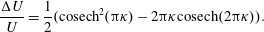 $$\begin{eqnarray}\frac{\unicode[STIX]{x0394}U}{U}=\frac{1}{2}(\text{cosech}^{2}(\unicode[STIX]{x03C0}\unicode[STIX]{x1D705})-2\unicode[STIX]{x03C0}\unicode[STIX]{x1D705}\text{cosech}(2\unicode[STIX]{x03C0}\unicode[STIX]{x1D705})).\end{eqnarray}$$
Here
 $U$
is the speed of the incompressible point vortex street and the compressible street speed is
$U$
is the speed of the incompressible point vortex street and the compressible street speed is
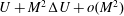 $U+M^{2}\unicode[STIX]{x0394}U+o(M^{2})$
, where
$U+M^{2}\unicode[STIX]{x0394}U+o(M^{2})$
, where
 $M=U/c_{s}$
is the Mach number (
$M=U/c_{s}$
is the Mach number (
 $c_{s}$
is the speed of sound in the fluid when at rest). This formula shows that compressible staggered point vortex streets of aspect ratio below a critical value of
$c_{s}$
is the speed of sound in the fluid when at rest). This formula shows that compressible staggered point vortex streets of aspect ratio below a critical value of
 $\unicode[STIX]{x1D705}=0.38187$
speed up compared to their incompressible counterparts, those of aspect ratios above this value travel more slowly. Here we investigate how the finite size of the vortex cores affects this result within a hollow vortex model of the cores.
$\unicode[STIX]{x1D705}=0.38187$
speed up compared to their incompressible counterparts, those of aspect ratios above this value travel more slowly. Here we investigate how the finite size of the vortex cores affects this result within a hollow vortex model of the cores.
The main finding of this paper is that compressible hollow vortex streets, with a fixed aspect ratio
 $\unicode[STIX]{x1D705}$
, can both speed up and slow down relative to the incompressible counterpart and that which eventuality occurs depends on the size of the vortex cores.
$\unicode[STIX]{x1D705}$
, can both speed up and slow down relative to the incompressible counterpart and that which eventuality occurs depends on the size of the vortex cores.
We view this study as adding to a small but growing collection of results in the literature giving evidence of the existence of transonic flows with embedded vortices (Barsony-Nagy et al. Reference Barsony-Nagy, Er-El and Yungster1987; Moore & Pullin Reference Moore and Pullin1987; Ardalan et al. Reference Ardalan, Meiron and Pullin1995; Leppington Reference Leppington2006; Crowdy & Krishnamurthy Reference Crowdy and Krishnamurthy2017). The analysis is expected to have relevance, for example, to more general studies of wave-like problems where acoustic energy is scattered, or generated, by vortex wakes (see Leppington (Reference Leppington2006) for a discussion of such problems where a Rayleigh–Jansen expansion akin to that developed here forms part of a matched asymptotic analysis of a more general wave problem).
The mathematical approach of this paper is different from that of Ardalan et al. (Reference Ardalan, Meiron and Pullin1995), and we do not use Chaplygin’s equation. Rather, we offer a new mathematical approach based on the idea of combining a complex variable formulation of the perturbation scheme – referred to as the Imai–Lamla formulation (Jacob Reference Jacob1959; Pai Reference Pai1959) – with conformal mapping to describe the shape of the unknown, or free, boundaries of the vortices. The Imai–Lamla formula was developed by Imai in his investigations of compressibility in flow around a cylinder with circulation (Imai Reference Imai1938, Reference Imai1941, Reference Imai1942; Jacob Reference Jacob1959). Barsony-Nagy et al. (Reference Barsony-Nagy, Er-El and Yungster1987) applied the method to obtain solutions for weakly compressible flow past an obstacle in the presence of point vortices (the compressible Föppl vortex pair). The latter study does not, however, use conformal mapping since the obstacle boundary is just a circle. In a two-dimensional setting, conformal mapping is a natural tool for free boundary analyses where the shape must be found as part of the solution. To the best of our knowledge, it has not previously been employed to study compressible vortices.
We focus here only on the staggered vortex street solutions found by Crowdy & Green (Reference Crowdy and Green2011). This is for two reasons. First, staggered streets are more commonly observed in bluff-body wakes (Williamson Reference Williamson1996). Second, we expect the results for unstaggered vortex streets – especially for vortices of small average radius relative to the period of the street – to follow the qualitative trends observed for isolated vortex pairs already studied in detail by Moore & Pullin (Reference Moore and Pullin1987) and Leppington (Reference Leppington2006). Extending this analysis to unstaggered street configurations should be a routine exercise requiring only minor changes.
2 The incompressible staggered hollow vortex street
For steady incompressible motion of an inviscid fluid, it is known (Saffman Reference Saffman1992) that, in a two-dimensional irrotational flow, a streamfunction
 $\unicode[STIX]{x1D713}(x,y)$
and a velocity potential
$\unicode[STIX]{x1D713}(x,y)$
and a velocity potential
 $\unicode[STIX]{x1D719}(x,y)$
exist satisfying the Cauchy–Riemann equations
$\unicode[STIX]{x1D719}(x,y)$
exist satisfying the Cauchy–Riemann equations
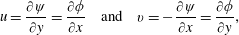 $$\begin{eqnarray}u={\displaystyle \frac{\unicode[STIX]{x2202}\unicode[STIX]{x1D713}}{\unicode[STIX]{x2202}y}}={\displaystyle \frac{\unicode[STIX]{x2202}\unicode[STIX]{x1D719}}{\unicode[STIX]{x2202}x}}\quad \text{and}\quad v=-{\displaystyle \frac{\unicode[STIX]{x2202}\unicode[STIX]{x1D713}}{\unicode[STIX]{x2202}x}}={\displaystyle \frac{\unicode[STIX]{x2202}\unicode[STIX]{x1D719}}{\unicode[STIX]{x2202}y}},\end{eqnarray}$$
where the velocity field is denoted by
 $(u,v)$
. It follows that
$(u,v)$
. It follows that
 $\unicode[STIX]{x1D719}(x,y)$
and
$\unicode[STIX]{x1D719}(x,y)$
and
 $\unicode[STIX]{x1D713}(x,y)$
are harmonic functions. One can introduce the complex potential
$\unicode[STIX]{x1D713}(x,y)$
are harmonic functions. One can introduce the complex potential
 $f(z)\equiv \unicode[STIX]{x1D719}+\text{i}\unicode[STIX]{x1D713}$
, which is an analytic function of the complex variable
$f(z)\equiv \unicode[STIX]{x1D719}+\text{i}\unicode[STIX]{x1D713}$
, which is an analytic function of the complex variable
 $z=x+\text{i}y$
. The (complex) velocity field is then given by its derivative:
$z=x+\text{i}y$
. The (complex) velocity field is then given by its derivative:
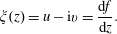 $$\begin{eqnarray}\unicode[STIX]{x1D709}(z)=u-\text{i}v={\displaystyle \frac{\text{d}f}{\text{d}z}}.\end{eqnarray}$$

Figure 1. Conformal mapping
 $z_{0}(\unicode[STIX]{x1D701})$
from the preimage cut annulus
$z_{0}(\unicode[STIX]{x1D701})$
from the preimage cut annulus
 $\unicode[STIX]{x1D70C}_{0}<|\unicode[STIX]{x1D701}|<1$
to a typical period window of a staggered hollow vortex street. The two sides of the branch cut joining
$\unicode[STIX]{x1D70C}_{0}<|\unicode[STIX]{x1D701}|<1$
to a typical period window of a staggered hollow vortex street. The two sides of the branch cut joining
 $\unicode[STIX]{x1D6FC}_{0}$
and
$\unicode[STIX]{x1D6FC}_{0}$
and
 $\unicode[STIX]{x1D6FD}_{0}$
are mapped by
$\unicode[STIX]{x1D6FD}_{0}$
are mapped by
 $z_{0}(\unicode[STIX]{x1D701})$
to the two edges of the period window. The two circles
$z_{0}(\unicode[STIX]{x1D701})$
to the two edges of the period window. The two circles
 $|\unicode[STIX]{x1D701}|=\unicode[STIX]{x1D70C}_{0},1$
each map to one of the hollow vortex boundaries. Shown on the right is the incompressible solution of Crowdy & Green (Reference Crowdy and Green2011) described by (2.4) with parameters
$|\unicode[STIX]{x1D701}|=\unicode[STIX]{x1D70C}_{0},1$
each map to one of the hollow vortex boundaries. Shown on the right is the incompressible solution of Crowdy & Green (Reference Crowdy and Green2011) described by (2.4) with parameters
 $L=\unicode[STIX]{x1D6E4}=1,\unicode[STIX]{x1D70C}_{0}=0.28,\unicode[STIX]{x1D6FC}_{0}=0.347,\unicode[STIX]{x1D6FD}_{0}=-0.806,\unicode[STIX]{x1D6FE}_{1}=-0.615$
and
$L=\unicode[STIX]{x1D6E4}=1,\unicode[STIX]{x1D70C}_{0}=0.28,\unicode[STIX]{x1D6FC}_{0}=0.347,\unicode[STIX]{x1D6FD}_{0}=-0.806,\unicode[STIX]{x1D6FE}_{1}=-0.615$
and
 $\unicode[STIX]{x1D6FE}_{2}=0.456$
, corresponding to a street travelling with speed
$\unicode[STIX]{x1D6FE}_{2}=0.456$
, corresponding to a street travelling with speed
 $U=0.316$
.
$U=0.316$
.
The incompressible solutions for staggered hollow vortex streets, comprising vortices with period
 $L$
and circulation
$L$
and circulation
 $\pm \unicode[STIX]{x1D6E4}$
travelling at speed
$\pm \unicode[STIX]{x1D6E4}$
travelling at speed
 $U$
, were found as a function of a parametric conformal mapping variable
$U$
, were found as a function of a parametric conformal mapping variable
 $\unicode[STIX]{x1D701}$
from the annulus shown in figure 1 by Crowdy & Green (Reference Crowdy and Green2011). The solutions for staggered streets travelling with speed
$\unicode[STIX]{x1D701}$
from the annulus shown in figure 1 by Crowdy & Green (Reference Crowdy and Green2011). The solutions for staggered streets travelling with speed
 $U\neq 0$
can be written
$U\neq 0$
can be written
 $$\begin{eqnarray}\displaystyle & \displaystyle f=f_{0}(\unicode[STIX]{x1D701})=\frac{\text{i}LU}{2\unicode[STIX]{x03C0}}\log \left[\frac{|\unicode[STIX]{x1D6FC}_{0}|P(\unicode[STIX]{x1D701}/\unicode[STIX]{x1D6FC}_{0},\unicode[STIX]{x1D70C}_{0})P(\unicode[STIX]{x1D701}\unicode[STIX]{x1D6FD}_{0},\unicode[STIX]{x1D70C}_{0})}{|\unicode[STIX]{x1D6FD}_{0}|P(\unicode[STIX]{x1D701}\unicode[STIX]{x1D6FC}_{0},\unicode[STIX]{x1D70C}_{0})P(\unicode[STIX]{x1D701}/\unicode[STIX]{x1D6FD}_{0},\unicode[STIX]{x1D70C}_{0})}\right]-\frac{\text{i}\unicode[STIX]{x1D6E4}}{2\unicode[STIX]{x03C0}}\log \unicode[STIX]{x1D701}, & \displaystyle\end{eqnarray}$$
 $$\begin{eqnarray}\displaystyle & \displaystyle z=z_{0}(\unicode[STIX]{x1D701})=-\frac{\text{i}L}{2\unicode[STIX]{x03C0}}\left[\log \left[\frac{P(\unicode[STIX]{x1D701}/\unicode[STIX]{x1D6FC}_{0},\unicode[STIX]{x1D70C}_{0})}{P(\unicode[STIX]{x1D701}/\unicode[STIX]{x1D6FD}_{0},\unicode[STIX]{x1D70C}_{0})}\right]-\unicode[STIX]{x1D712}\log \left[\frac{P(\unicode[STIX]{x1D701}\unicode[STIX]{x1D6FC}_{0},\unicode[STIX]{x1D70C}_{0})}{P(\unicode[STIX]{x1D701}\unicode[STIX]{x1D6FD}_{0},\unicode[STIX]{x1D70C}_{0})}\right]\right]+\frac{\text{i}L}{4\unicode[STIX]{x03C0}}\log (\unicode[STIX]{x1D6FD}_{0}/\unicode[STIX]{x1D6FC}_{0}),\qquad & \displaystyle\end{eqnarray}$$
 $$\begin{eqnarray}\displaystyle & \displaystyle u-\text{i}v=\frac{\text{d}f}{\text{d}z}=\unicode[STIX]{x1D709}_{0}(\unicode[STIX]{x1D701})=-\frac{U\unicode[STIX]{x1D70C}_{0}}{\sqrt{\unicode[STIX]{x1D712}}\unicode[STIX]{x1D701}}\left[\frac{P(\unicode[STIX]{x1D701}/\unicode[STIX]{x1D6FE}_{1},\unicode[STIX]{x1D70C}_{0})P(\unicode[STIX]{x1D701}/\unicode[STIX]{x1D6FE}_{2},\unicode[STIX]{x1D70C}_{0})}{P(\unicode[STIX]{x1D701}\unicode[STIX]{x1D6FE}_{1},\unicode[STIX]{x1D70C}_{0})P(\unicode[STIX]{x1D701}\unicode[STIX]{x1D6FE}_{2},\unicode[STIX]{x1D70C}_{0})}\right], & \displaystyle\end{eqnarray}$$
where
 $f$
is the complex potential. In these formulae,
$f$
is the complex potential. In these formulae,
 $$\begin{eqnarray}\unicode[STIX]{x1D712}\equiv \frac{\unicode[STIX]{x1D70C}_{0}^{2}}{\unicode[STIX]{x1D6FC}_{0}^{2}}\left[\frac{P^{2}(\unicode[STIX]{x1D6FC}_{0}/\unicode[STIX]{x1D6FE}_{1},\unicode[STIX]{x1D70C}_{0})P^{2}(\unicode[STIX]{x1D6FC}_{0}/\unicode[STIX]{x1D6FE}_{2},\unicode[STIX]{x1D70C}_{0})}{P^{2}(\unicode[STIX]{x1D6FC}_{0}\unicode[STIX]{x1D6FE}_{1},\unicode[STIX]{x1D70C}_{0})P^{2}(\unicode[STIX]{x1D6FC}_{0}\unicode[STIX]{x1D6FE}_{2},\unicode[STIX]{x1D70C}_{0})}\right]\end{eqnarray}$$
and the real parameters
 $\unicode[STIX]{x1D70C}_{0},\unicode[STIX]{x1D6FC}_{0},\unicode[STIX]{x1D6FD}_{0},\unicode[STIX]{x1D6FE}_{1}$
and
$\unicode[STIX]{x1D70C}_{0},\unicode[STIX]{x1D6FC}_{0},\unicode[STIX]{x1D6FD}_{0},\unicode[STIX]{x1D6FE}_{1}$
and
 $\unicode[STIX]{x1D6FE}_{2}$
satisfy
$\unicode[STIX]{x1D6FE}_{2}$
satisfy
 $$\begin{eqnarray}\unicode[STIX]{x1D6FC}_{0}\unicode[STIX]{x1D6FD}_{0}=-\unicode[STIX]{x1D70C}_{0}=\unicode[STIX]{x1D6FE}_{1}\unicode[STIX]{x1D6FE}_{2}\end{eqnarray}$$
as well as the two conditions
 $$\begin{eqnarray}\displaystyle & \displaystyle 0=-K(\unicode[STIX]{x1D6FE}_{1}\unicode[STIX]{x1D6FC}_{0},\unicode[STIX]{x1D70C}_{0})-\unicode[STIX]{x1D712}K(\unicode[STIX]{x1D6FC}_{0}/\unicode[STIX]{x1D6FE}_{1},\unicode[STIX]{x1D70C}_{0})+K(\unicode[STIX]{x1D6FE}_{1}\unicode[STIX]{x1D6FD}_{0},\unicode[STIX]{x1D70C}_{0})+\unicode[STIX]{x1D712}K(\unicode[STIX]{x1D6FD}_{0}/\unicode[STIX]{x1D6FE}_{1},\unicode[STIX]{x1D70C}_{0}), & \displaystyle\end{eqnarray}$$
 $$\begin{eqnarray}\displaystyle & \displaystyle \frac{\unicode[STIX]{x1D6E4}}{LU}=K(\unicode[STIX]{x1D6FE}_{1}/\unicode[STIX]{x1D6FC}_{0},\unicode[STIX]{x1D70C}_{0})-K(\unicode[STIX]{x1D6FE}_{1}/\unicode[STIX]{x1D6FD}_{0},\unicode[STIX]{x1D70C}_{0})-K(\unicode[STIX]{x1D6FE}_{1}\unicode[STIX]{x1D6FC}_{0},\unicode[STIX]{x1D70C}_{0})+K(\unicode[STIX]{x1D6FE}_{1}\unicode[STIX]{x1D6FD}_{0},\unicode[STIX]{x1D70C}_{0}). & \displaystyle\end{eqnarray}$$
The constant speed
 $q_{0}$
of the fluid on both hollow vortex boundaries can be shown to be
$q_{0}$
of the fluid on both hollow vortex boundaries can be shown to be
 $$\begin{eqnarray}q_{0}=\frac{U}{\sqrt{\unicode[STIX]{x1D712}}}.\end{eqnarray}$$
For given
 $\unicode[STIX]{x1D6E4},L$
and
$\unicode[STIX]{x1D6E4},L$
and
 $U$
, these solutions depend on five mathematical parameters:
$U$
, these solutions depend on five mathematical parameters:
 $\unicode[STIX]{x1D70C}_{0},\unicode[STIX]{x1D6FC}_{0},\unicode[STIX]{x1D6FD}_{0},\unicode[STIX]{x1D6FE}_{1}$
and
$\unicode[STIX]{x1D70C}_{0},\unicode[STIX]{x1D6FC}_{0},\unicode[STIX]{x1D6FD}_{0},\unicode[STIX]{x1D6FE}_{1}$
and
 $\unicode[STIX]{x1D6FE}_{2}$
. We can fix one of these parameters,
$\unicode[STIX]{x1D6FE}_{2}$
. We can fix one of these parameters,
 $\unicode[STIX]{x1D70C}_{0}$
say, and this corresponds to picking the area of the hollow vortices making up the street (note that they all have the same area). The four remaining parameters are then determined by solving the four equations (2.7)–(2.9). Constructed this way, the centroid of the vortices, and hence the aspect ratio of the street, will emerge from the solution. Alternatively, one can assign
$\unicode[STIX]{x1D70C}_{0}$
say, and this corresponds to picking the area of the hollow vortices making up the street (note that they all have the same area). The four remaining parameters are then determined by solving the four equations (2.7)–(2.9). Constructed this way, the centroid of the vortices, and hence the aspect ratio of the street, will emerge from the solution. Alternatively, one can assign
 $\unicode[STIX]{x1D6E4}$
and
$\unicode[STIX]{x1D6E4}$
and
 $L$
and insist that the aspect ratio of the street takes a particular value; this geometrical condition replaces (2.9) as one of the equations to determine the four parameters
$L$
and insist that the aspect ratio of the street takes a particular value; this geometrical condition replaces (2.9) as one of the equations to determine the four parameters
 $\unicode[STIX]{x1D6FC}_{0},\unicode[STIX]{x1D6FD}_{0},\unicode[STIX]{x1D6FE}_{1}$
and
$\unicode[STIX]{x1D6FC}_{0},\unicode[STIX]{x1D6FD}_{0},\unicode[STIX]{x1D6FE}_{1}$
and
 $\unicode[STIX]{x1D6FE}_{2}$
. In such cases, equation (2.9) is used a posteriori to determine the associated street speed
$\unicode[STIX]{x1D6FE}_{2}$
. In such cases, equation (2.9) is used a posteriori to determine the associated street speed
 $U$
.
$U$
.
The special functions
 $P(\unicode[STIX]{x1D701},\unicode[STIX]{x1D70C}_{0})$
and
$P(\unicode[STIX]{x1D701},\unicode[STIX]{x1D70C}_{0})$
and
 $K(\unicode[STIX]{x1D701},\unicode[STIX]{x1D70C}_{0})$
, which are related to the so-called Schottky–Klein prime function of the annulus
$K(\unicode[STIX]{x1D701},\unicode[STIX]{x1D70C}_{0})$
, which are related to the so-called Schottky–Klein prime function of the annulus
 $\unicode[STIX]{x1D70C}_{0}<|\unicode[STIX]{x1D701}|<1$
, are defined in appendix A, where their important properties are also given.
$\unicode[STIX]{x1D70C}_{0}<|\unicode[STIX]{x1D701}|<1$
, are defined in appendix A, where their important properties are also given.
The expression for
 $z_{0}(\unicode[STIX]{x1D701})$
in (2.4) differs from that given by Crowdy & Green (Reference Crowdy and Green2011), where it was reported as an indefinite integral. During the course of this compressible flow analysis, it was realized that the latter integral can be calculated explicitly, leading to (2.4). Appendix B gives details of how to perform this integration. It requires knowledge of the properties of
$z_{0}(\unicode[STIX]{x1D701})$
in (2.4) differs from that given by Crowdy & Green (Reference Crowdy and Green2011), where it was reported as an indefinite integral. During the course of this compressible flow analysis, it was realized that the latter integral can be calculated explicitly, leading to (2.4). Appendix B gives details of how to perform this integration. It requires knowledge of the properties of
 $P(\unicode[STIX]{x1D701},\unicode[STIX]{x1D70C}_{0})$
and
$P(\unicode[STIX]{x1D701},\unicode[STIX]{x1D70C}_{0})$
and
 $K(\unicode[STIX]{x1D701},\unicode[STIX]{x1D70C}_{0})$
given in appendix A.
$K(\unicode[STIX]{x1D701},\unicode[STIX]{x1D70C}_{0})$
given in appendix A.
The two boundary circles
 $|\unicode[STIX]{x1D701}|=\unicode[STIX]{x1D70C}_{0},1$
are transplanted under the mapping function
$|\unicode[STIX]{x1D701}|=\unicode[STIX]{x1D70C}_{0},1$
are transplanted under the mapping function
 $z=z_{0}(\unicode[STIX]{x1D701})$
to the two hollow vortex boundaries; see figure 1. Owing to the presence of the logarithmic branch points at
$z=z_{0}(\unicode[STIX]{x1D701})$
to the two hollow vortex boundaries; see figure 1. Owing to the presence of the logarithmic branch points at
 $\unicode[STIX]{x1D6FC}_{0}$
and
$\unicode[STIX]{x1D6FC}_{0}$
and
 $\unicode[STIX]{x1D6FD}_{0}$
of the mapping
$\unicode[STIX]{x1D6FD}_{0}$
of the mapping
 $z_{0}(\unicode[STIX]{x1D701})$
, the latter function is required to be single-valued and one-to-one everywhere in the annulus
$z_{0}(\unicode[STIX]{x1D701})$
, the latter function is required to be single-valued and one-to-one everywhere in the annulus
 $\unicode[STIX]{x1D70C}_{0}<|\unicode[STIX]{x1D701}|<1$
outside a branch cut between
$\unicode[STIX]{x1D70C}_{0}<|\unicode[STIX]{x1D701}|<1$
outside a branch cut between
 $\unicode[STIX]{x1D6FC}_{0}$
and
$\unicode[STIX]{x1D6FC}_{0}$
and
 $\unicode[STIX]{x1D6FD}_{0}$
. The images of the two sides of that branch cut under the mapping
$\unicode[STIX]{x1D6FD}_{0}$
. The images of the two sides of that branch cut under the mapping
 $z_{0}(\unicode[STIX]{x1D701})$
will be the two sides of the period window. For convenience we refer to the region in the annulus
$z_{0}(\unicode[STIX]{x1D701})$
will be the two sides of the period window. For convenience we refer to the region in the annulus
 $\unicode[STIX]{x1D70C}_{0}<|\unicode[STIX]{x1D701}|<1$
exterior to this branch cut as the ‘cut annulus’. The mapping satisfies the functional identity
$\unicode[STIX]{x1D70C}_{0}<|\unicode[STIX]{x1D701}|<1$
exterior to this branch cut as the ‘cut annulus’. The mapping satisfies the functional identity
 $$\begin{eqnarray}z_{0}(-\unicode[STIX]{x1D70C}_{0}/\unicode[STIX]{x1D701})=-z_{0}(\unicode[STIX]{x1D701}),\end{eqnarray}$$
which ensures the rotational symmetry of the two vortices about the origin.
3 Compressible flow equations
When the flow becomes compressible, a new variable enters the analysis: the density of the fluid
 $\unicode[STIX]{x1D708}(z,\overline{z})$
, which is now a function of space (and, for unsteady flow, also of time). Conservation of mass, for a steady flow, requires that
$\unicode[STIX]{x1D708}(z,\overline{z})$
, which is now a function of space (and, for unsteady flow, also of time). Conservation of mass, for a steady flow, requires that
 $$\begin{eqnarray}\frac{\unicode[STIX]{x2202}(\unicode[STIX]{x1D708}u)}{\unicode[STIX]{x2202}x}+\frac{\unicode[STIX]{x2202}(\unicode[STIX]{x1D708}v)}{\unicode[STIX]{x2202}y}=0,\end{eqnarray}$$
which is clearly invariant to a rescaling of the fluid density. If we let
 $\unicode[STIX]{x1D708}_{0}$
be the (constant) incompressible density, then we have the freedom to specify this at our convenience, and this will be done later.
$\unicode[STIX]{x1D708}_{0}$
be the (constant) incompressible density, then we have the freedom to specify this at our convenience, and this will be done later.
As for the dynamics, it is known (Saffman Reference Saffman1992) that, in the absence of body forces, the steady vorticity equation for a barotropic fluid – defined to be one for which pressure is just a function of density, i.e.
 $p=p(\unicode[STIX]{x1D708})$
– admits an irrotational flow as a possible solution; this means that
$p=p(\unicode[STIX]{x1D708})$
– admits an irrotational flow as a possible solution; this means that
 $\unicode[STIX]{x1D714}=\unicode[STIX]{x2202}v/\unicode[STIX]{x2202}x-\unicode[STIX]{x2202}u/\unicode[STIX]{x2202}y=0$
. Here we will seek a solution for a steady compressible flow that is free of vorticity except for non-zero circulations around hollow vortices. Since the flow is still two-dimensional and irrotational, we can introduce a velocity potential
$\unicode[STIX]{x1D714}=\unicode[STIX]{x2202}v/\unicode[STIX]{x2202}x-\unicode[STIX]{x2202}u/\unicode[STIX]{x2202}y=0$
. Here we will seek a solution for a steady compressible flow that is free of vorticity except for non-zero circulations around hollow vortices. Since the flow is still two-dimensional and irrotational, we can introduce a velocity potential
 $\unicode[STIX]{x1D719}$
and a streamfunction
$\unicode[STIX]{x1D719}$
and a streamfunction
 $\unicode[STIX]{x1D713}$
, but these are now related by the modified system
$\unicode[STIX]{x1D713}$
, but these are now related by the modified system
 $$\begin{eqnarray}u={\displaystyle \frac{\unicode[STIX]{x1D708}_{0}}{\unicode[STIX]{x1D708}}}{\displaystyle \frac{\unicode[STIX]{x2202}\unicode[STIX]{x1D713}}{\unicode[STIX]{x2202}y}}={\displaystyle \frac{\unicode[STIX]{x2202}\unicode[STIX]{x1D719}}{\unicode[STIX]{x2202}x}}\quad \text{and}\quad v=-{\displaystyle \frac{\unicode[STIX]{x1D708}_{0}}{\unicode[STIX]{x1D708}}}{\displaystyle \frac{\unicode[STIX]{x2202}\unicode[STIX]{x1D713}}{\unicode[STIX]{x2202}x}}={\displaystyle \frac{\unicode[STIX]{x2202}\unicode[STIX]{x1D719}}{\unicode[STIX]{x2202}y}};\end{eqnarray}$$
 $\unicode[STIX]{x1D719}(x,y)$
and
$\unicode[STIX]{x1D719}(x,y)$
and
 $\unicode[STIX]{x1D713}(x,y)$
are no longer harmonic. We can still define the complex potential as
$\unicode[STIX]{x1D713}(x,y)$
are no longer harmonic. We can still define the complex potential as
 $f(z,\overline{z})=\unicode[STIX]{x1D719}+\text{i}\unicode[STIX]{x1D713}$
, but it is not an analytic function of
$f(z,\overline{z})=\unicode[STIX]{x1D719}+\text{i}\unicode[STIX]{x1D713}$
, but it is not an analytic function of
 $z$
. Despite this loss of analyticity, we can continue to employ the two independent variables,
$z$
. Despite this loss of analyticity, we can continue to employ the two independent variables,
 $z$
and
$z$
and
 $\overline{z}$
, where the overbar denotes complex conjugation. On noting that
$\overline{z}$
, where the overbar denotes complex conjugation. On noting that
 $$\begin{eqnarray}\frac{\unicode[STIX]{x2202}}{\unicode[STIX]{x2202}z}=\frac{1}{2}\left[\frac{\unicode[STIX]{x2202}}{\unicode[STIX]{x2202}x}-\text{i}\frac{\unicode[STIX]{x2202}}{\unicode[STIX]{x2202}y}\right],\quad \frac{\unicode[STIX]{x2202}}{\unicode[STIX]{x2202}\overline{z}}=\frac{1}{2}\left[\frac{\unicode[STIX]{x2202}}{\unicode[STIX]{x2202}x}+\text{i}\frac{\unicode[STIX]{x2202}}{\unicode[STIX]{x2202}y}\right],\end{eqnarray}$$
it is readily shown from (3.2) that
 $$\begin{eqnarray}2\frac{\unicode[STIX]{x2202}f}{\unicode[STIX]{x2202}\overline{z}}=\left(1-\frac{\unicode[STIX]{x1D708}}{\unicode[STIX]{x1D708}_{0}}\right)(u+\text{i}v),\quad 2\frac{\unicode[STIX]{x2202}\overline{f}}{\unicode[STIX]{x2202}z}=\left(1+\frac{\unicode[STIX]{x1D708}}{\unicode[STIX]{x1D708}_{0}}\right)(u+\text{i}v).\end{eqnarray}$$
Division of these two equations leads to
 $$\begin{eqnarray}\frac{\unicode[STIX]{x2202}f}{\unicode[STIX]{x2202}\overline{z}}=B(\unicode[STIX]{x1D708})\frac{\unicode[STIX]{x2202}\overline{f}}{\unicode[STIX]{x2202}\overline{z}},\end{eqnarray}$$
where
 $$\begin{eqnarray}B(\unicode[STIX]{x1D708})=\frac{1-\unicode[STIX]{x1D708}/\unicode[STIX]{x1D708}_{0}}{1+\unicode[STIX]{x1D708}/\unicode[STIX]{x1D708}_{0}},\end{eqnarray}$$
which is a real-valued function of the density
 $\unicode[STIX]{x1D708}(z,\overline{z})$
. Clearly
$\unicode[STIX]{x1D708}(z,\overline{z})$
. Clearly
 $B(\unicode[STIX]{x1D708})=0$
when the flow is incompressible, reducing
$B(\unicode[STIX]{x1D708})=0$
when the flow is incompressible, reducing
 $f(z,\overline{z})$
to an analytic function. The complex velocity field
$f(z,\overline{z})$
to an analytic function. The complex velocity field
 $\unicode[STIX]{x1D709}(z,\bar{z})\equiv u-\text{i}v$
can be written either in terms of the complex potential as
$\unicode[STIX]{x1D709}(z,\bar{z})\equiv u-\text{i}v$
can be written either in terms of the complex potential as
 $$\begin{eqnarray}\unicode[STIX]{x1D709}(z,\bar{z})=u-\text{i}v=\frac{\unicode[STIX]{x2202}\unicode[STIX]{x1D719}}{\unicode[STIX]{x2202}x}-\text{i}\frac{\unicode[STIX]{x2202}\unicode[STIX]{x1D719}}{\unicode[STIX]{x2202}y}=\frac{\unicode[STIX]{x2202}}{\unicode[STIX]{x2202}z}(f+\overline{f})\end{eqnarray}$$
or, on use of (3.5), in terms of the complex potential and fluid density as
 $$\begin{eqnarray}\unicode[STIX]{x1D709}(z,\bar{z})={\displaystyle \frac{\unicode[STIX]{x2202}f}{\unicode[STIX]{x2202}z}}(1+B(\unicode[STIX]{x1D708})).\end{eqnarray}$$
We consider the fluid to be in isentropic flow, meaning that the pressure and density are related by
 $p=k\unicode[STIX]{x1D708}^{\unicode[STIX]{x1D6FE}}$
, where
$p=k\unicode[STIX]{x1D708}^{\unicode[STIX]{x1D6FE}}$
, where
 $k$
and
$k$
and
 $\unicode[STIX]{x1D6FE}>1$
are constants determined by the thermodynamical properties of the fluid (Jacob Reference Jacob1959; Pai Reference Pai1959; von Mises Reference von Mises2004). For steady flow of an inviscid barotropic fluid in two dimensions, a Bernoulli equation can be established (Saffman Reference Saffman1992):
$\unicode[STIX]{x1D6FE}>1$
are constants determined by the thermodynamical properties of the fluid (Jacob Reference Jacob1959; Pai Reference Pai1959; von Mises Reference von Mises2004). For steady flow of an inviscid barotropic fluid in two dimensions, a Bernoulli equation can be established (Saffman Reference Saffman1992):
 $$\begin{eqnarray}{\displaystyle \frac{|\unicode[STIX]{x1D709}|^{2}}{2}}+\int ^{\unicode[STIX]{x1D708}}\frac{\text{d}p}{\text{d}\tilde{\unicode[STIX]{x1D708}}}\frac{\text{d}\tilde{\unicode[STIX]{x1D708}}}{\tilde{\unicode[STIX]{x1D708}}}=\text{const.},\end{eqnarray}$$
where
 $\tilde{\unicode[STIX]{x1D708}}$
is a dummy integration variable. On substitution of the assumed pressure–density relationship into the Bernoulli equation (3.9), we can eliminate the pressure to obtain an equation relating the velocity and the density of the fluid:
$\tilde{\unicode[STIX]{x1D708}}$
is a dummy integration variable. On substitution of the assumed pressure–density relationship into the Bernoulli equation (3.9), we can eliminate the pressure to obtain an equation relating the velocity and the density of the fluid:
 $$\begin{eqnarray}{\displaystyle \frac{|\unicode[STIX]{x1D709}|^{2}}{2}}+{\displaystyle \frac{k\unicode[STIX]{x1D6FE}\unicode[STIX]{x1D708}^{\unicode[STIX]{x1D6FE}-1}}{\unicode[STIX]{x1D6FE}-1}}={\displaystyle \frac{k\unicode[STIX]{x1D6FE}\unicode[STIX]{x1D708}_{s}^{\unicode[STIX]{x1D6FE}-1}}{\unicode[STIX]{x1D6FE}-1}},\end{eqnarray}$$
where
 $\unicode[STIX]{x1D708}_{s}$
is the (constant) density at the stagnation point in the flow. Since
$\unicode[STIX]{x1D708}_{s}$
is the (constant) density at the stagnation point in the flow. Since
 $\unicode[STIX]{x1D708}(z,\overline{z})>0$
, we will have a maximum value
$\unicode[STIX]{x1D708}(z,\overline{z})>0$
, we will have a maximum value
 $|\unicode[STIX]{x1D709}|_{max}$
for the speed:
$|\unicode[STIX]{x1D709}|_{max}$
for the speed:
 $$\begin{eqnarray}|\unicode[STIX]{x1D709}|^{2}<|\unicode[STIX]{x1D709}|_{max}^{2}={\displaystyle \frac{2k\unicode[STIX]{x1D6FE}\unicode[STIX]{x1D708}_{s}^{\unicode[STIX]{x1D6FE}-1}}{\unicode[STIX]{x1D6FE}-1}}={\displaystyle \frac{2c_{s}^{2}}{\unicode[STIX]{x1D6FE}-1}},\end{eqnarray}$$
where
 $c_{s}$
is the speed of sound at the stagnation point; the speed of sound is defined by
$c_{s}$
is the speed of sound at the stagnation point; the speed of sound is defined by
 $$\begin{eqnarray}c^{2}\equiv \frac{\text{d}p}{\text{d}\unicode[STIX]{x1D708}}=k\unicode[STIX]{x1D6FE}\unicode[STIX]{x1D708}^{\unicode[STIX]{x1D6FE}-1}.\end{eqnarray}$$
The presence of an upper limit on the speed of fluid flow immediately rules out point vortices as solutions of the compressible flow equations; this is one reason for employing the hollow vortex model since it is a desingularization of the point vortex that is particularly convenient for compressible flow analysis. Returning to the Bernoulli equation (3.10), in terms of
 $c_{s}$
, we find
$c_{s}$
, we find
 $$\begin{eqnarray}\left[{\displaystyle \frac{\unicode[STIX]{x1D6FE}-1}{2c_{s}^{2}}}\right]|\unicode[STIX]{x1D709}|^{2}=1-\left[{\displaystyle \frac{\unicode[STIX]{x1D708}}{\unicode[STIX]{x1D708}_{s}}}\right]^{\unicode[STIX]{x1D6FE}-1}.\end{eqnarray}$$
We see from this equation that the density has a maximum value, namely
 $\unicode[STIX]{x1D708}_{s}$
:
$\unicode[STIX]{x1D708}_{s}$
:
 $\unicode[STIX]{x1D708}(z,\overline{z})<\unicode[STIX]{x1D708}_{s}$
.
$\unicode[STIX]{x1D708}(z,\overline{z})<\unicode[STIX]{x1D708}_{s}$
.
We now have a closed system of equations governing the steady, two-dimensional, compressible and irrotational flow of an inviscid isentropic fluid: equation (3.5), which is complex-valued, and the Bernoulli equation (3.10) or (3.13), which is real. These two equations are to be solved for the complex potential and the density field.
4 Small-Mach-number perturbation: the Rayleigh–Jansen expansion
Let
 $M$
be the Mach number, defined by
$M$
be the Mach number, defined by
 $M=V_{0}/c_{s}$
, where
$M=V_{0}/c_{s}$
, where
 $V_{0}$
is the fluid speed at some suitably chosen point in the flow. In the general theory of Rayleigh–Jansen expansions, one considers flows that are weakly compressible so that
$V_{0}$
is the fluid speed at some suitably chosen point in the flow. In the general theory of Rayleigh–Jansen expansions, one considers flows that are weakly compressible so that
 $M\ll 1$
(Jacob Reference Jacob1959; Pai Reference Pai1959). Rayleigh–Jansen expansions for the complex potential and the velocity field take the form
$M\ll 1$
(Jacob Reference Jacob1959; Pai Reference Pai1959). Rayleigh–Jansen expansions for the complex potential and the velocity field take the form
 $$\begin{eqnarray}f(z,\overline{z})=f_{0}(z)+M^{2}f_{1}(z,\overline{z})+\cdots \,,\quad \unicode[STIX]{x1D709}(z,\overline{z})=\unicode[STIX]{x1D709}_{0}(z)+M^{2}\unicode[STIX]{x1D709}_{1}(z,\overline{z})+\cdots \,,\end{eqnarray}$$
where we use dots to denote the higher-order terms in an expansion in powers of
 $M^{2}$
. The complex potential
$M^{2}$
. The complex potential
 $f_{0}(z)$
and complex velocity
$f_{0}(z)$
and complex velocity
 $\unicode[STIX]{x1D709}_{0}(z)$
are those associated with some incompressible base-state flow of interest. From the Bernoulli equation (3.13) we find
$\unicode[STIX]{x1D709}_{0}(z)$
are those associated with some incompressible base-state flow of interest. From the Bernoulli equation (3.13) we find
 $$\begin{eqnarray}\displaystyle {\displaystyle \frac{\unicode[STIX]{x1D708}}{\unicode[STIX]{x1D708}_{s}}} & = & \displaystyle \left[1-\left({\displaystyle \frac{\unicode[STIX]{x1D6FE}-1}{2}}\right){\displaystyle \frac{|\unicode[STIX]{x1D709}|^{2}}{c_{s}^{2}}}\right]^{(1/\unicode[STIX]{x1D6FE}-1)}=\left[1-\left({\displaystyle \frac{\unicode[STIX]{x1D6FE}-1}{2}}\right)\,{\displaystyle \frac{|\unicode[STIX]{x1D709}|^{2}}{V_{0}^{2}}}\,M^{2}\right]^{(1/\unicode[STIX]{x1D6FE}-1)}\nonumber\\ \displaystyle & = & \displaystyle 1-{\displaystyle \frac{1}{2}}\,{\displaystyle \frac{|\unicode[STIX]{x1D709}_{0}|^{2}}{V_{0}^{2}}}\,M^{2}+\cdots \,.\end{eqnarray}$$
To find the Rayleigh–Jansen expansion of (3.5), consider the function
 $B(\unicode[STIX]{x1D708})$
defined in (3.6). Without loss of generality, we set
$B(\unicode[STIX]{x1D708})$
defined in (3.6). Without loss of generality, we set
 $\unicode[STIX]{x1D708}_{0}=\unicode[STIX]{x1D708}_{s}$
, leading to
$\unicode[STIX]{x1D708}_{0}=\unicode[STIX]{x1D708}_{s}$
, leading to
 $$\begin{eqnarray}1-{\displaystyle \frac{\unicode[STIX]{x1D708}}{\unicode[STIX]{x1D708}_{s}}}={\displaystyle \frac{1}{2}}\,{\displaystyle \frac{|\unicode[STIX]{x1D709}_{0}|^{2}}{V_{0}^{2}}}\,M^{2}+\cdots \,,\quad 1+{\displaystyle \frac{\unicode[STIX]{x1D708}}{\unicode[STIX]{x1D708}_{s}}}=2\left[1-{\displaystyle \frac{1}{4}}\,{\displaystyle \frac{|\unicode[STIX]{x1D709}_{0}|^{2}}{V_{0}^{2}}}\,M^{2}+\cdots \,\right],\end{eqnarray}$$
so that
 $$\begin{eqnarray}B(\unicode[STIX]{x1D708})={\displaystyle \frac{1}{4}}\,{\displaystyle \frac{|\unicode[STIX]{x1D709}_{0}|^{2}}{V_{0}^{2}}}\,M^{2}+\cdots \,.\end{eqnarray}$$
Substituting the Rayleigh–Jansen expansion (4.1) for the complex potential into (3.5) gives
 $$\begin{eqnarray}\frac{\unicode[STIX]{x2202}f_{0}}{\unicode[STIX]{x2202}\overline{z}}+M^{2}\frac{\unicode[STIX]{x2202}f_{1}}{\unicode[STIX]{x2202}\overline{z}}+\cdots =B(\unicode[STIX]{x1D708})\frac{\unicode[STIX]{x2202}\overline{f}_{0}}{\unicode[STIX]{x2202}\overline{z}}+M^{2}B(\unicode[STIX]{x1D708})\frac{\unicode[STIX]{x2202}\overline{f}_{1}}{\unicode[STIX]{x2202}\overline{z}}+\cdots \,.\end{eqnarray}$$
On use of (4.4), and on equating coefficients of the powers of
 $M^{2}$
, we find
$M^{2}$
, we find
 $$\begin{eqnarray}\frac{\unicode[STIX]{x2202}f_{0}}{\unicode[STIX]{x2202}\overline{z}}=0,\quad \frac{\unicode[STIX]{x2202}f_{1}}{\unicode[STIX]{x2202}\overline{z}}={\displaystyle \frac{1}{4}}\,{\displaystyle \frac{|\unicode[STIX]{x1D709}_{0}|^{2}}{V_{0}^{2}}}\frac{\unicode[STIX]{x2202}\overline{f}_{0}}{\unicode[STIX]{x2202}\overline{z}}.\end{eqnarray}$$
The first equation reminds us that the incompressible complex potential is an analytic function; the second equation gives us a relation between the first-order complex potential and the incompressible solution. We can integrate the latter equation with respect to
 $\overline{z}$
:
$\overline{z}$
:
 $$\begin{eqnarray}f_{1}(z,\overline{z})={\displaystyle \frac{1}{4V_{0}^{2}}}\unicode[STIX]{x1D709}_{0}(z)\overline{I(z)}+g(z),\end{eqnarray}$$
where
 $$\begin{eqnarray}I(z)=\int ^{z}\unicode[STIX]{x1D709}_{0}(\tilde{z})^{2}\,\text{d}\tilde{z},\end{eqnarray}$$
and where
 $g(z)$
has to be found. We refer to (4.7) as the Imai–Lamla formula: it gives an explicit formula, up to an unknown function
$g(z)$
has to be found. We refer to (4.7) as the Imai–Lamla formula: it gives an explicit formula, up to an unknown function
 $g(z)$
, for the first-order correction to the complex potential in terms of the leading-order incompressible solution.
$g(z)$
, for the first-order correction to the complex potential in terms of the leading-order incompressible solution.
To find the Rayleigh–Jansen expansion for the velocity, we substitute the Rayleigh–Jansen expansion for the complex potential (4.1) and (4.4) into (3.7):
 $$\begin{eqnarray}\unicode[STIX]{x1D709}(z,\overline{z})=\frac{\text{d}f_{0}}{\text{d}z}+M^{2}\left[{\displaystyle \frac{1}{4V_{0}^{2}}}\left(\unicode[STIX]{x1D709}_{0}(z)\right)^{2}\overline{\unicode[STIX]{x1D709}_{0}(z)}+\frac{\unicode[STIX]{x2202}f_{1}}{\unicode[STIX]{x2202}z}\right]+\cdots \,,\end{eqnarray}$$
where we have used the fact, following immediately from (4.8), that
 $\text{d}I(z)/\text{d}z=\unicode[STIX]{x1D709}_{0}^{2}(z)$
. We recognize immediately, on comparison of (4.1) and (4.9), that
$\text{d}I(z)/\text{d}z=\unicode[STIX]{x1D709}_{0}^{2}(z)$
. We recognize immediately, on comparison of (4.1) and (4.9), that
 $$\begin{eqnarray}\unicode[STIX]{x1D709}_{1}(z,\overline{z})={\displaystyle \frac{1}{4V_{0}^{2}}}\left(\unicode[STIX]{x1D709}_{0}(z)\right)^{2}\overline{\unicode[STIX]{x1D709}_{0}(z)}+\frac{\unicode[STIX]{x2202}f_{1}}{\unicode[STIX]{x2202}z}.\end{eqnarray}$$
It will be expedient to perform the Rayleigh–Jansen analysis about the incompressible hollow vortex solutions with all functions considered as functions of a subsidiary parametric
 $\unicode[STIX]{x1D701}$
-plane, where
$\unicode[STIX]{x1D701}$
-plane, where
 $z$
and
$z$
and
 $\unicode[STIX]{x1D701}$
are related by a conformal mapping, which we will denote by
$\unicode[STIX]{x1D701}$
are related by a conformal mapping, which we will denote by
 $$\begin{eqnarray}z=z_{0}(\unicode[STIX]{x1D701})+M^{2}z_{1}(\unicode[STIX]{x1D701})+\cdots \,,\end{eqnarray}$$
where, just as for the complex potential and complex velocity in (4.1), we seek the form of the compressible perturbation to the conformal mapping
 $z_{0}(\unicode[STIX]{x1D701})$
which is relevant to the incompressible solution. The first-order correction
$z_{0}(\unicode[STIX]{x1D701})$
which is relevant to the incompressible solution. The first-order correction
 $z_{1}(\unicode[STIX]{x1D701})$
will encode the change in shape of the hollow vortices due to the effects of compressibility.
$z_{1}(\unicode[STIX]{x1D701})$
will encode the change in shape of the hollow vortices due to the effects of compressibility.
It is important to explain a notational convention adopted for the remainder of this paper. We continue to use the function names
 $f_{0},~f_{1},\unicode[STIX]{x1D709}_{0},\unicode[STIX]{x1D709}_{1}$
even though we now take them to be functions of the parametric
$f_{0},~f_{1},\unicode[STIX]{x1D709}_{0},\unicode[STIX]{x1D709}_{1}$
even though we now take them to be functions of the parametric
 $\unicode[STIX]{x1D701}$
variable rather than of
$\unicode[STIX]{x1D701}$
variable rather than of
 $z$
. Strictly speaking, new function names should be introduced, but this abuse of notation should not cause confusion.
$z$
. Strictly speaking, new function names should be introduced, but this abuse of notation should not cause confusion.
The Imai–Lamla integral (4.8), written as a function of
 $\unicode[STIX]{x1D701}$
, will be denoted by
$\unicode[STIX]{x1D701}$
, will be denoted by
 $$\begin{eqnarray}{\mathcal{I}}(\unicode[STIX]{x1D701})=\int ^{\unicode[STIX]{x1D701}}\frac{f_{0}^{\prime }(\tilde{\unicode[STIX]{x1D701}})^{2}}{z_{0}^{\prime }(\tilde{\unicode[STIX]{x1D701}})}\,\text{d}\tilde{\unicode[STIX]{x1D701}},\end{eqnarray}$$
where we will use the prime notation to denote derivatives of analytic functions with respect to their arguments. The first-order correction to the complex potential is then
 $$\begin{eqnarray}f_{1}=\frac{1}{4V_{0}^{2}}\left[\unicode[STIX]{x1D709}_{0}(\unicode[STIX]{x1D701})\overline{{\mathcal{I}}(\unicode[STIX]{x1D701})}\right]+G(\unicode[STIX]{x1D701}),\end{eqnarray}$$
where the function
 $G(\unicode[STIX]{x1D701})$
must be found. With this change of variables, it follows that
$G(\unicode[STIX]{x1D701})$
must be found. With this change of variables, it follows that
 $$\begin{eqnarray}\unicode[STIX]{x1D709}(\unicode[STIX]{x1D701},\overline{\unicode[STIX]{x1D701}})=\unicode[STIX]{x1D709}_{0}(\unicode[STIX]{x1D701})+M^{2}\left[\frac{1}{z_{0}^{\prime }(\unicode[STIX]{x1D701})}\frac{\unicode[STIX]{x2202}}{\unicode[STIX]{x2202}\unicode[STIX]{x1D701}}(f_{1}+\overline{f_{1}})-\unicode[STIX]{x1D709}_{0}(\unicode[STIX]{x1D701})\frac{z_{1}^{\prime }(\unicode[STIX]{x1D701})}{z_{0}^{\prime }(\unicode[STIX]{x1D701})}\right]+\cdots\end{eqnarray}$$
and, on comparison with (4.1),
 $$\begin{eqnarray}\unicode[STIX]{x1D709}_{1}(\unicode[STIX]{x1D701},\overline{\unicode[STIX]{x1D701}})=\unicode[STIX]{x1D709}_{0}(\unicode[STIX]{x1D701})\left[\,\frac{1}{f_{0}^{\prime }(\unicode[STIX]{x1D701})}\frac{\unicode[STIX]{x2202}}{\unicode[STIX]{x2202}\unicode[STIX]{x1D701}}(f_{1}+\overline{f_{1}})-\frac{z_{1}^{\prime }(\unicode[STIX]{x1D701})}{z_{0}^{\prime }(\unicode[STIX]{x1D701})}\right].\end{eqnarray}$$
As an instructive illustration of the new approach adopted here, supplementary material is available at https://doi.org/10.1017/jfm.2017.821, in which we use the Imai–Lamla method and the techniques of conformal mapping to rederive the Rayleigh–Jansen expansion about the single incompressible hollow vortex row found by Baker et al. (Reference Baker, Saffman and Sheffield1976). A different but equivalent analysis has been performed by Ardalan et al. (Reference Ardalan, Meiron and Pullin1995) using a hodograph formulation and Chaplygin’s equation. We check our results against the latter work and thus provide a conceptual check on the new approach. The analysis to follow is a natural extension, to the staggered hollow vortex street, of that given in the supplementary material for the single hollow vortex row.
5 Rayleigh–Jansen expansion: the staggered hollow vortex street
We now consider a Rayleigh–Jansen expansion about the incompressible solution of Crowdy & Green (Reference Crowdy and Green2011). We choose the velocity scale
 $V_{0}$
in the definition of the Mach number to be the speed of the incompressible hollow vortex street
$V_{0}$
in the definition of the Mach number to be the speed of the incompressible hollow vortex street
 $U$
from § 2 (we assume that
$U$
from § 2 (we assume that
 $U\neq 0$
, otherwise a different choice of Mach number would be more appropriate). The complex potential and complex velocity will be perturbed as in (4.1) and, for a fixed value of the street aspect ratio and area of the vortices, we expect the speed of the street to be altered to
$U\neq 0$
, otherwise a different choice of Mach number would be more appropriate). The complex potential and complex velocity will be perturbed as in (4.1) and, for a fixed value of the street aspect ratio and area of the vortices, we expect the speed of the street to be altered to
 $$\begin{eqnarray}U+M^{2}\unicode[STIX]{x0394}U.\end{eqnarray}$$
The key objective of the analysis to follow is to determine
 $\unicode[STIX]{x0394}U$
.
$\unicode[STIX]{x0394}U$
.
5.1 Perturbation of the conformal mapping
Since the incompressible vortices are perturbed, we must assume that the conformally equivalent cut annulus to the compressible vortices is also perturbed to
 $$\begin{eqnarray}\unicode[STIX]{x1D70C}<|\unicode[STIX]{x1D701}|<1,\quad \unicode[STIX]{x1D70C}=\unicode[STIX]{x1D70C}_{0}+M^{2}\hat{\unicode[STIX]{x1D70C}}+\cdots \,,\end{eqnarray}$$
with the preimages of
 $\infty ^{+}$
and
$\infty ^{+}$
and
 $\infty ^{-}$
becoming
$\infty ^{-}$
becoming
 $$\begin{eqnarray}\unicode[STIX]{x1D6FC}=\unicode[STIX]{x1D6FC}_{0}+M^{2}\hat{\unicode[STIX]{x1D6FC}}+\cdots \,,\quad \unicode[STIX]{x1D6FD}=\unicode[STIX]{x1D6FD}_{0}+M^{2}\hat{\unicode[STIX]{x1D6FD}}+\cdots \,,\end{eqnarray}$$
for parameters
 $\hat{\unicode[STIX]{x1D6FC}}$
and
$\hat{\unicode[STIX]{x1D6FC}}$
and
 $\hat{\unicode[STIX]{x1D6FD}}$
to be determined. In order that the perturbed mapping corresponds to an
$\hat{\unicode[STIX]{x1D6FD}}$
to be determined. In order that the perturbed mapping corresponds to an
 $L$
-periodic structure, we write it in the form
$L$
-periodic structure, we write it in the form
 $$\begin{eqnarray}z(\unicode[STIX]{x1D701})=-\frac{\text{i}L}{2\unicode[STIX]{x03C0}}\log \left[\frac{P(\unicode[STIX]{x1D701}/\unicode[STIX]{x1D6FC},\unicode[STIX]{x1D70C}_{0})}{P(\unicode[STIX]{x1D701}/\unicode[STIX]{x1D6FD},\unicode[STIX]{x1D70C}_{0})}\right]+\tilde{z}_{0}(\unicode[STIX]{x1D701})+M^{2}\tilde{z}_{1}(\unicode[STIX]{x1D701})+\cdots \,,\end{eqnarray}$$
where we define
 $\tilde{z}_{0}(\unicode[STIX]{x1D701})$
via the relation
$\tilde{z}_{0}(\unicode[STIX]{x1D701})$
via the relation
 $$\begin{eqnarray}z_{0}(\unicode[STIX]{x1D701})=-\frac{\text{i}L}{2\unicode[STIX]{x03C0}}\log \left[\frac{P(\unicode[STIX]{x1D701}/\unicode[STIX]{x1D6FC}_{0},\unicode[STIX]{x1D70C}_{0})}{P(\unicode[STIX]{x1D701}/\unicode[STIX]{x1D6FD}_{0},\unicode[STIX]{x1D70C}_{0})}\right]+\tilde{z}_{0}(\unicode[STIX]{x1D701}).\end{eqnarray}$$
The quantity
 $\tilde{z}_{1}(\unicode[STIX]{x1D701})$
is analytic and single-valued in the perturbed cut annulus (5.2). On linearizing in
$\tilde{z}_{1}(\unicode[STIX]{x1D701})$
is analytic and single-valued in the perturbed cut annulus (5.2). On linearizing in
 $M^{2}$
:
$M^{2}$
:
 $$\begin{eqnarray}P(\unicode[STIX]{x1D701}/\unicode[STIX]{x1D6FC},\unicode[STIX]{x1D70C}_{0})=P(\unicode[STIX]{x1D701}/\unicode[STIX]{x1D6FC}_{0},\unicode[STIX]{x1D70C}_{0})\left[1-M^{2}\frac{\hat{\unicode[STIX]{x1D6FC}}}{\unicode[STIX]{x1D6FC}_{0}}K(\unicode[STIX]{x1D701}/\unicode[STIX]{x1D6FC}_{0},\unicode[STIX]{x1D70C}_{0})\right].\end{eqnarray}$$
Therefore
 $$\begin{eqnarray}\displaystyle -\frac{\text{i}L}{2\unicode[STIX]{x03C0}}\log \left[\frac{P(\unicode[STIX]{x1D701}/\unicode[STIX]{x1D6FC},\unicode[STIX]{x1D70C}_{0})}{P(\unicode[STIX]{x1D701}/\unicode[STIX]{x1D6FD},\unicode[STIX]{x1D70C}_{0})}\right] & = & \displaystyle -\frac{\text{i}L}{2\unicode[STIX]{x03C0}}\log \left[\frac{P(\unicode[STIX]{x1D701}/\unicode[STIX]{x1D6FC}_{0},\unicode[STIX]{x1D70C}_{0})}{P(\unicode[STIX]{x1D701}/\unicode[STIX]{x1D6FD}_{0},\unicode[STIX]{x1D70C}_{0})}\right]\nonumber\\ \displaystyle & & \displaystyle +\,M^{2}\left(\frac{\text{i}L}{2\unicode[STIX]{x03C0}}\right)\left[\frac{\hat{\unicode[STIX]{x1D6FC}}}{\unicode[STIX]{x1D6FC}_{0}}K(\unicode[STIX]{x1D701}/\unicode[STIX]{x1D6FC}_{0},\unicode[STIX]{x1D70C}_{0})-\frac{\hat{\unicode[STIX]{x1D6FD}}}{\unicode[STIX]{x1D6FD}_{0}}K(\unicode[STIX]{x1D701}/\unicode[STIX]{x1D6FD}_{0},\unicode[STIX]{x1D70C}_{0})\right]+\cdots \nonumber\\ \displaystyle & & \displaystyle\end{eqnarray}$$
implying that
 $$\begin{eqnarray}z=z_{0}(\unicode[STIX]{x1D701})+M^{2}\left(\frac{\text{i}L}{2\unicode[STIX]{x03C0}}\right)\left[\frac{\hat{\unicode[STIX]{x1D6FC}}}{\unicode[STIX]{x1D6FC}_{0}}K(\unicode[STIX]{x1D701}/\unicode[STIX]{x1D6FC}_{0},\unicode[STIX]{x1D70C}_{0})-\frac{\hat{\unicode[STIX]{x1D6FD}}}{\unicode[STIX]{x1D6FD}_{0}}K(\unicode[STIX]{x1D701}/\unicode[STIX]{x1D6FD}_{0},\unicode[STIX]{x1D70C}_{0})\right]+M^{2}\tilde{z}_{1}(\unicode[STIX]{x1D701})+\cdots \,.\end{eqnarray}$$
On comparison with
 $$\begin{eqnarray}z(\unicode[STIX]{x1D701})=z_{0}(\unicode[STIX]{x1D701})+M^{2}z_{1}(\unicode[STIX]{x1D701})+\cdots \,,\end{eqnarray}$$
we infer that
 $$\begin{eqnarray}z_{1}(\unicode[STIX]{x1D701})={\mathcal{Z}}_{s}(\unicode[STIX]{x1D701})+\tilde{z}_{1}(\unicode[STIX]{x1D701}),\end{eqnarray}$$
where
 $$\begin{eqnarray}{\mathcal{Z}}_{s}(\unicode[STIX]{x1D701})\equiv \left(\frac{\text{i}L}{2\unicode[STIX]{x03C0}}\right)\left[\frac{\hat{\unicode[STIX]{x1D6FC}}}{\unicode[STIX]{x1D6FC}_{0}}K(\unicode[STIX]{x1D701}/\unicode[STIX]{x1D6FC}_{0},\unicode[STIX]{x1D70C}_{0})-\frac{\hat{\unicode[STIX]{x1D6FD}}}{\unicode[STIX]{x1D6FD}_{0}}K(\unicode[STIX]{x1D701}/\unicode[STIX]{x1D6FD}_{0},\unicode[STIX]{x1D70C}_{0})\right].\end{eqnarray}$$
This first-order correction
 $z_{1}(\unicode[STIX]{x1D701})$
to the conformal mapping has simple poles at
$z_{1}(\unicode[STIX]{x1D701})$
to the conformal mapping has simple poles at
 $\unicode[STIX]{x1D6FC}_{0}$
and
$\unicode[STIX]{x1D6FC}_{0}$
and
 $\unicode[STIX]{x1D6FD}_{0}$
.
$\unicode[STIX]{x1D6FD}_{0}$
.
5.2 The Imai–Lamla integral
For the leading-order solution, we have assumed that the origin is at the centre of the period window of interest, and that the staggered vortices are rotations of each other by angle
 $\unicode[STIX]{x03C0}$
. It is natural to suppose that it will be possible to find a compressible staggered vortex street solution with this same symmetry.
$\unicode[STIX]{x03C0}$
. It is natural to suppose that it will be possible to find a compressible staggered vortex street solution with this same symmetry.
We need to evaluate the integral
 ${\mathcal{I}}(\unicode[STIX]{x1D701})$
defined in (4.12). Remarkably, it is possible to do this in closed form. Appendix C explains how to derive the following expression:
${\mathcal{I}}(\unicode[STIX]{x1D701})$
defined in (4.12). Remarkably, it is possible to do this in closed form. Appendix C explains how to derive the following expression:
 $$\begin{eqnarray}{\mathcal{I}}(\unicode[STIX]{x1D701})=-\frac{\text{i}LU^{2}}{2\unicode[STIX]{x03C0}}\left[\log \left[\frac{P(\unicode[STIX]{x1D701}/\unicode[STIX]{x1D6FC}_{0},\unicode[STIX]{x1D70C}_{0})}{P(\unicode[STIX]{x1D701}/\unicode[STIX]{x1D6FD}_{0},\unicode[STIX]{x1D70C}_{0})}\right]-\frac{1}{\unicode[STIX]{x1D712}}\log \left[\frac{P(\unicode[STIX]{x1D701}\unicode[STIX]{x1D6FC}_{0},\unicode[STIX]{x1D70C}_{0})}{P(\unicode[STIX]{x1D701}\unicode[STIX]{x1D6FD}_{0},\unicode[STIX]{x1D70C}_{0})}\right]\right].\end{eqnarray}$$
Now
 $f_{1}$
takes the form (4.13), where
$f_{1}$
takes the form (4.13), where
 $G(\unicode[STIX]{x1D701})$
is to be determined. To ensure that the velocity field is
$G(\unicode[STIX]{x1D701})$
is to be determined. To ensure that the velocity field is
 $L$
-periodic, we can choose
$L$
-periodic, we can choose
 $$\begin{eqnarray}G(\unicode[STIX]{x1D701})=-\frac{1}{4U^{2}}\unicode[STIX]{x1D709}_{0}(\unicode[STIX]{x1D701}){\mathcal{I}}(\unicode[STIX]{x1D701})+{\mathcal{G}}(\unicode[STIX]{x1D701}),\end{eqnarray}$$
where
 ${\mathcal{G}}(\unicode[STIX]{x1D701})$
is single-valued in the cut annulus (but it may have isolated singularities). Note from (5.12) that
${\mathcal{G}}(\unicode[STIX]{x1D701})$
is single-valued in the cut annulus (but it may have isolated singularities). Note from (5.12) that
 $$\begin{eqnarray}{\mathcal{I}}(\unicode[STIX]{x1D701})=U^{2}z_{0}(\unicode[STIX]{x1D701})+\frac{\text{i}LU^{2}}{2\unicode[STIX]{x03C0}}\left[\frac{1}{\unicode[STIX]{x1D712}}-\unicode[STIX]{x1D712}\right]\log \left[\frac{P(\unicode[STIX]{x1D701}\unicode[STIX]{x1D6FC}_{0},\unicode[STIX]{x1D70C}_{0})}{P(\unicode[STIX]{x1D701}\unicode[STIX]{x1D6FD}_{0},\unicode[STIX]{x1D70C}_{0})}\right],\end{eqnarray}$$
so that, since
 $\unicode[STIX]{x1D709}_{0}\rightarrow -U$
as
$\unicode[STIX]{x1D709}_{0}\rightarrow -U$
as
 $z\rightarrow \infty$
,
$z\rightarrow \infty$
,
 $$\begin{eqnarray}-\frac{1}{4U^{2}}\unicode[STIX]{x1D709}_{0}(\unicode[STIX]{x1D701}){\mathcal{I}}(\unicode[STIX]{x1D701})\sim \frac{U}{4}z,\quad \text{as }z\rightarrow \infty .\end{eqnarray}$$
Hence, from (4.15), any first-order correction to the speed at infinity will come only from
 ${\mathcal{G}}(\unicode[STIX]{x1D701})$
. With the choice (5.13),
${\mathcal{G}}(\unicode[STIX]{x1D701})$
. With the choice (5.13),
 $$\begin{eqnarray}f_{1}=\frac{1}{4U^{2}}\unicode[STIX]{x1D709}_{0}(\unicode[STIX]{x1D701})\left\{\overline{{\mathcal{I}}(\unicode[STIX]{x1D701})}-{\mathcal{I}}(\unicode[STIX]{x1D701})\right\}+{\mathcal{G}}(\unicode[STIX]{x1D701}),\end{eqnarray}$$
where
 $$\begin{eqnarray}\overline{{\mathcal{I}}(\unicode[STIX]{x1D701})}-{\mathcal{I}}(\unicode[STIX]{x1D701})=\frac{\text{i}LU^{2}}{2\unicode[STIX]{x03C0}}\left[\log \left|\frac{P(\unicode[STIX]{x1D701}/\unicode[STIX]{x1D6FC}_{0},\unicode[STIX]{x1D70C}_{0})}{P(\unicode[STIX]{x1D701}/\unicode[STIX]{x1D6FD}_{0},\unicode[STIX]{x1D70C}_{0})}\right|^{2}-\frac{1}{\unicode[STIX]{x1D712}}\log \left|\frac{P(\unicode[STIX]{x1D701}\unicode[STIX]{x1D6FC}_{0},\unicode[STIX]{x1D70C}_{0})}{P(\unicode[STIX]{x1D701}\unicode[STIX]{x1D6FD}_{0},\unicode[STIX]{x1D70C}_{0})}\right|^{2}\right],\end{eqnarray}$$
whence it can be checked that the associated velocity field is
 $L$
-periodic. For the perturbed problem, we expect, in the far field, the effects of compressibility to have decayed, and the flow to be irrotational, except for the change in speed of the street. Hence as
$L$
-periodic. For the perturbed problem, we expect, in the far field, the effects of compressibility to have decayed, and the flow to be irrotational, except for the change in speed of the street. Hence as
 $z\rightarrow \infty$
,
$z\rightarrow \infty$
,
 $$\begin{eqnarray}f_{0}+M^{2}f_{1}\rightarrow -(U+M^{2}\unicode[STIX]{x0394}U)z=-(U+M^{2}\unicode[STIX]{x0394}U)(z_{0}+M^{2}z_{1})+\cdots \,,\end{eqnarray}$$
where we have used (5.1). But since
 $f_{1}\sim {\mathcal{G}}(\unicode[STIX]{x1D701})$
as
$f_{1}\sim {\mathcal{G}}(\unicode[STIX]{x1D701})$
as
 $z\rightarrow \infty$
, then we identify, at
$z\rightarrow \infty$
, then we identify, at
 $O(M^{2})$
,
$O(M^{2})$
,
 $$\begin{eqnarray}{\mathcal{G}}\sim -\unicode[STIX]{x0394}Uz_{0}-Uz_{1},\quad \text{as }z\rightarrow \infty .\end{eqnarray}$$
Motivated by this we make the choice
 $$\begin{eqnarray}{\mathcal{G}}(\unicode[STIX]{x1D701})=\unicode[STIX]{x1D709}_{0}{\mathcal{Z}}_{s}+\frac{\unicode[STIX]{x0394}U}{U}\left[f_{0}+\frac{\text{i}\unicode[STIX]{x1D6E4}}{2\unicode[STIX]{x03C0}}\log \unicode[STIX]{x1D701}\right]+\tilde{{\mathcal{G}}}(\unicode[STIX]{x1D701}),\end{eqnarray}$$
where
 $\tilde{{\mathcal{G}}}(\unicode[STIX]{x1D701})$
is analytic and single-valued in the annulus, which, given that
$\tilde{{\mathcal{G}}}(\unicode[STIX]{x1D701})$
is analytic and single-valued in the annulus, which, given that
 $f_{0}\rightarrow -Uz_{0}$
,
$f_{0}\rightarrow -Uz_{0}$
,
 $z_{1}={\mathcal{Z}}_{s}+\tilde{z}_{1}$
and
$z_{1}={\mathcal{Z}}_{s}+\tilde{z}_{1}$
and
 $\unicode[STIX]{x1D709}_{0}\rightarrow -U$
, has precisely the expected far-field asymptotics (5.19). The term in square brackets in (5.20) warrants some explanation. It includes a logarithmic term that negates a similar term appearing in
$\unicode[STIX]{x1D709}_{0}\rightarrow -U$
, has precisely the expected far-field asymptotics (5.19). The term in square brackets in (5.20) warrants some explanation. It includes a logarithmic term that negates a similar term appearing in
 $f_{0}$
and hence contributes no additional circulation around either of the vortices. This is necessary because we want the circulation of the compressible vortices to be the same as the incompressible solution. From (4.14) the
$f_{0}$
and hence contributes no additional circulation around either of the vortices. This is necessary because we want the circulation of the compressible vortices to be the same as the incompressible solution. From (4.14) the
 $O(M^{2})$
change in circulation around the vortex that is the image of
$O(M^{2})$
change in circulation around the vortex that is the image of
 $|\unicode[STIX]{x1D701}|=1$
due to the perturbation from the first term on the right-hand side of (5.16) is
$|\unicode[STIX]{x1D701}|=1$
due to the perturbation from the first term on the right-hand side of (5.16) is
 $$\begin{eqnarray}\text{Re}\left[\oint _{|\unicode[STIX]{x1D701}|=1}(\unicode[STIX]{x1D709}_{1}z_{0}^{\prime }(\unicode[STIX]{x1D701})+\unicode[STIX]{x1D709}_{0}z_{1}^{\prime }(\unicode[STIX]{x1D701}))\,\text{d}\unicode[STIX]{x1D701}\right]=\text{Re}\left[\oint _{|\unicode[STIX]{x1D701}|=1}\text{d}\unicode[STIX]{x1D709}_{0}\,(\overline{{\mathcal{I}}(\unicode[STIX]{x1D701})}-{\mathcal{I}}(\unicode[STIX]{x1D701}))+(\overline{\unicode[STIX]{x1D709}_{0}}-\unicode[STIX]{x1D709}_{0})\,\text{d}{\mathcal{I}}\right]=0,\end{eqnarray}$$
where the last equality follows because the integral can be shown to be an integral of a total derivative of a single-valued function around the closed curve
 $|\unicode[STIX]{x1D701}|=1$
.
$|\unicode[STIX]{x1D701}|=1$
.
5.3 Streamline condition for
 ${\mathcal{G}}(\unicode[STIX]{x1D701})$

The leading-order kinematic boundary condition that each hollow vortex boundary is a streamline is
 $$\begin{eqnarray}\text{Im}[f_{0}]=\left\{\begin{array}{@{}ll@{}}0, & \text{ on }|\unicode[STIX]{x1D701}|=1,\\ c_{0}, & \text{ on }|\unicode[STIX]{x1D701}|=\unicode[STIX]{x1D70C}_{0},\end{array}\right.\end{eqnarray}$$
where
 $$\begin{eqnarray}c_{0}=\frac{LU}{2\unicode[STIX]{x03C0}}\log \biggl|\frac{\unicode[STIX]{x1D6FC}_{0}}{\unicode[STIX]{x1D6FD}_{0}}\biggr|-\frac{\unicode[STIX]{x1D6E4}}{2\unicode[STIX]{x03C0}}\log \unicode[STIX]{x1D70C}_{0}\end{eqnarray}$$
is a constant. For the compressible vortices, this condition is perturbed to
 $$\begin{eqnarray}\text{Im}[f_{0}+M^{2}f_{1}+\cdots \,]=\left\{\begin{array}{@{}ll@{}}0, & \text{ on }|\unicode[STIX]{x1D701}|=1,\\ c_{0}+M^{2}c_{1}, & \text{ on }|\unicode[STIX]{x1D701}|=\unicode[STIX]{x1D70C}_{0}+M^{2}\hat{\unicode[STIX]{x1D70C}},\end{array}\right.\end{eqnarray}$$
where the value of
 $c_{1}$
is to be determined. On
$c_{1}$
is to be determined. On
 $|\unicode[STIX]{x1D701}|=\unicode[STIX]{x1D70C}=\unicode[STIX]{x1D70C}_{0}+M^{2}\hat{\unicode[STIX]{x1D70C}}$
,
$|\unicode[STIX]{x1D701}|=\unicode[STIX]{x1D70C}=\unicode[STIX]{x1D70C}_{0}+M^{2}\hat{\unicode[STIX]{x1D70C}}$
,
 $$\begin{eqnarray}f_{0}(\unicode[STIX]{x1D701})=f_{0}(\unicode[STIX]{x1D701})\biggl|_{|\unicode[STIX]{x1D701}|=\unicode[STIX]{x1D70C}_{0}}+~M^{2}\frac{\hat{\unicode[STIX]{x1D70C}}}{\unicode[STIX]{x1D70C}_{0}}\unicode[STIX]{x1D701}f_{0}^{\prime }(\unicode[STIX]{x1D701})\biggr|_{|\unicode[STIX]{x1D701}|=\unicode[STIX]{x1D70C}_{0}}+\cdots \,,\end{eqnarray}$$
which, on use of the leading-order boundary conditions (5.22), gives
 $$\begin{eqnarray}\text{Im}[f_{1}]=\left\{\begin{array}{@{}ll@{}}0, & \text{ on }|\unicode[STIX]{x1D701}|=1,\\ c_{1}-\displaystyle \frac{\hat{\unicode[STIX]{x1D70C}}}{\unicode[STIX]{x1D70C}_{0}}\text{Im}[\unicode[STIX]{x1D701}f_{0}^{\prime }(\unicode[STIX]{x1D701})], & \text{ on }|\unicode[STIX]{x1D701}|=\unicode[STIX]{x1D70C}_{0}.\end{array}\right.\end{eqnarray}$$
However, on substitution of (5.20) into (5.16) and the result into (5.26), we arrive at the modified Schwarz problem (Crowdy Reference Crowdy2008b
) in the concentric annulus
 $\unicode[STIX]{x1D70C}_{0}<|\unicode[STIX]{x1D701}|<1$
,
$\unicode[STIX]{x1D70C}_{0}<|\unicode[STIX]{x1D701}|<1$
,
 $$\begin{eqnarray}\text{Re}[-\text{i}\tilde{{\mathcal{G}}}(\unicode[STIX]{x1D701})]=\left\{\begin{array}{@{}ll@{}}\displaystyle \frac{\unicode[STIX]{x0394}U}{U}g_{0}-\text{Im}[S(\unicode[STIX]{x1D701},\overline{\unicode[STIX]{x1D701}})]-\text{Im}[\unicode[STIX]{x1D709}_{0}{\mathcal{Z}}_{s}], & \text{ on }|\unicode[STIX]{x1D701}|=1,\\ c_{1}+\displaystyle \frac{\unicode[STIX]{x0394}U}{U}g_{1}-\displaystyle \frac{\hat{\unicode[STIX]{x1D70C}}}{\unicode[STIX]{x1D70C}_{0}}\text{Im}[\unicode[STIX]{x1D701}f_{0}^{\prime }(\unicode[STIX]{x1D701})]-\text{Im}[S(\unicode[STIX]{x1D701},\overline{\unicode[STIX]{x1D701}})]-\text{Im}[\unicode[STIX]{x1D709}_{0}{\mathcal{Z}}_{s}], & \text{ on }|\unicode[STIX]{x1D701}|=\unicode[STIX]{x1D70C}_{0},\end{array}\right.\end{eqnarray}$$
where we define
 $$\begin{eqnarray}S(\unicode[STIX]{x1D701},\overline{\unicode[STIX]{x1D701}})\equiv \frac{1}{4U^{2}}[\unicode[STIX]{x1D709}_{0}(\unicode[STIX]{x1D701})\{\overline{{\mathcal{I}}(\unicode[STIX]{x1D701})}-{\mathcal{I}}(\unicode[STIX]{x1D701})\}]\end{eqnarray}$$
and
 $$\begin{eqnarray}\text{Im}\left[f_{0}+\frac{\text{i}\unicode[STIX]{x1D6E4}}{2\unicode[STIX]{x03C0}}\log \unicode[STIX]{x1D701}\right]=\left\{\begin{array}{@{}ll@{}}0, & \text{ on }|\unicode[STIX]{x1D701}|=1,\\ g_{1}, & \text{ on }|\unicode[STIX]{x1D701}|=\unicode[STIX]{x1D70C}_{0},\end{array}\right.\end{eqnarray}$$
where
 $$\begin{eqnarray}g_{1}=\frac{LU}{2\unicode[STIX]{x03C0}}\log \biggl|\frac{\unicode[STIX]{x1D6FC}_{0}}{\unicode[STIX]{x1D6FD}_{0}}\biggr|.\end{eqnarray}$$
It is convenient to use the linearity of the problem and write the solution in the form
 $$\begin{eqnarray}\tilde{{\mathcal{G}}}(\unicode[STIX]{x1D701})=V_{1}(\unicode[STIX]{x1D701})+\frac{\hat{\unicode[STIX]{x1D6FC}}}{\unicode[STIX]{x1D6FC}_{0}}V_{2}(\unicode[STIX]{x1D701})+\frac{\hat{\unicode[STIX]{x1D6FD}}}{\unicode[STIX]{x1D6FD}_{0}}V_{3}(\unicode[STIX]{x1D701})+\frac{\unicode[STIX]{x0394}U}{U}V_{4}(\unicode[STIX]{x1D701})+\frac{\hat{\unicode[STIX]{x1D70C}}}{\unicode[STIX]{x1D70C}_{0}}V_{5}(\unicode[STIX]{x1D701}).\end{eqnarray}$$
Here
 $\{V_{j}(\unicode[STIX]{x1D701})\mid j=1,\ldots ,5\}$
are single-valued functions in the annulus
$\{V_{j}(\unicode[STIX]{x1D701})\mid j=1,\ldots ,5\}$
are single-valued functions in the annulus
 $\unicode[STIX]{x1D70C}_{0}<|\unicode[STIX]{x1D701}|<1$
and are defined, up to an additive real constant, by the modified Schwarz problems in the concentric annulus
$\unicode[STIX]{x1D70C}_{0}<|\unicode[STIX]{x1D701}|<1$
and are defined, up to an additive real constant, by the modified Schwarz problems in the concentric annulus
 $\unicode[STIX]{x1D70C}_{0}<|\unicode[STIX]{x1D701}|<1$
:
$\unicode[STIX]{x1D70C}_{0}<|\unicode[STIX]{x1D701}|<1$
:
 $$\begin{eqnarray}\left.\begin{array}{@{}c@{}}\begin{array}{@{}ll@{}}\text{Re}[-\text{i}V_{1}(\unicode[STIX]{x1D701})] & =\left\{\begin{array}{@{}ll@{}}-\text{Im}[S(\unicode[STIX]{x1D701},\overline{\unicode[STIX]{x1D701}})], & \text{ on }|\unicode[STIX]{x1D701}|=1,\\ -\text{Im}[S(\unicode[STIX]{x1D701},\overline{\unicode[STIX]{x1D701}})]+v_{1}, & \text{ on }|\unicode[STIX]{x1D701}|=\unicode[STIX]{x1D70C}_{0},\end{array}\right.\\ \text{Re}[-\text{i}V_{2}(\unicode[STIX]{x1D701})] & =\left\{\begin{array}{@{}ll@{}}-\displaystyle \text{Im}\left[\frac{\text{i}L}{2\unicode[STIX]{x03C0}}\unicode[STIX]{x1D709}_{0}(\unicode[STIX]{x1D701})K(\unicode[STIX]{x1D701}/\unicode[STIX]{x1D6FC}_{0},\unicode[STIX]{x1D70C}_{0})\right], & \text{ on }|\unicode[STIX]{x1D701}|=1,\\ -\displaystyle \text{Im}\left[\frac{\text{i}L}{2\unicode[STIX]{x03C0}}\unicode[STIX]{x1D709}_{0}(\unicode[STIX]{x1D701})K(\unicode[STIX]{x1D701}/\unicode[STIX]{x1D6FC}_{0},\unicode[STIX]{x1D70C}_{0})\right]+v_{2}, & \text{ on }|\unicode[STIX]{x1D701}|=\unicode[STIX]{x1D70C}_{0},\end{array}\right.\\ \text{Re}[-\text{i}V_{3}(\unicode[STIX]{x1D701})] & =\left\{\begin{array}{@{}ll@{}}\displaystyle \text{Im}\left[\frac{\text{i}L}{2\unicode[STIX]{x03C0}}\unicode[STIX]{x1D709}_{0}(\unicode[STIX]{x1D701})K(\unicode[STIX]{x1D701}/\unicode[STIX]{x1D6FD}_{0},\unicode[STIX]{x1D70C}_{0})\right], & \text{ on }|\unicode[STIX]{x1D701}|=1,\\ \displaystyle \text{Im}\left[\frac{\text{i}L}{2\unicode[STIX]{x03C0}}\unicode[STIX]{x1D709}_{0}(\unicode[STIX]{x1D701})K(\unicode[STIX]{x1D701}/\unicode[STIX]{x1D6FD}_{0},\unicode[STIX]{x1D70C}_{0})\right]+v_{3}, & \text{ on }|\unicode[STIX]{x1D701}|=\unicode[STIX]{x1D70C}_{0},\end{array}\right.\\ \text{Re}[-\text{i}V_{4}(\unicode[STIX]{x1D701})] & =\left\{\begin{array}{@{}ll@{}}0, & \text{ on }|\unicode[STIX]{x1D701}|=1,\\ g_{1}+v_{4}, & \text{ on }|\unicode[STIX]{x1D701}|=\unicode[STIX]{x1D70C}_{0},\end{array}\right.\\ \text{Re}[-\text{i}V_{5}(\unicode[STIX]{x1D701})] & =\left\{\begin{array}{@{}ll@{}}0, & \text{ on }|\unicode[STIX]{x1D701}|=1,\\ -\text{Im}[\unicode[STIX]{x1D701}f_{0}^{\prime }(\unicode[STIX]{x1D701})]+v_{5}, & \text{ on }|\unicode[STIX]{x1D701}|=\unicode[STIX]{x1D70C}_{0}.\end{array}\right.\end{array}\end{array}\right\}\end{eqnarray}$$
The real constants
 $\{v_{j}\mid j=1,\ldots ,5\}$
are determined by solvability conditions for each modified Schwarz problem. Appendix D contains a discussion of what is meant by the designation modified Schwarz problem in this case, and the solvability condition just mentioned; it also discusses various solution schemes. In this case, the solvability condition for
$\{v_{j}\mid j=1,\ldots ,5\}$
are determined by solvability conditions for each modified Schwarz problem. Appendix D contains a discussion of what is meant by the designation modified Schwarz problem in this case, and the solvability condition just mentioned; it also discusses various solution schemes. In this case, the solvability condition for
 $\tilde{G}(\unicode[STIX]{x1D701})$
is that
$\tilde{G}(\unicode[STIX]{x1D701})$
is that
 $$\begin{eqnarray}c_{1}=v_{1}+\frac{\hat{\unicode[STIX]{x1D6FC}}}{\unicode[STIX]{x1D6FC}_{0}}v_{2}+\frac{\hat{\unicode[STIX]{x1D6FD}}}{\unicode[STIX]{x1D6FD}_{0}}v_{3}+\frac{\unicode[STIX]{x0394}U}{U}v_{4}+\frac{\hat{\unicode[STIX]{x1D70C}}}{\unicode[STIX]{x1D70C}_{0}}v_{5},\end{eqnarray}$$
which merely determines
 $c_{1}$
and does not constitute any constraint on the as yet unknown parameters
$c_{1}$
and does not constitute any constraint on the as yet unknown parameters
 $\hat{\unicode[STIX]{x1D6FC}},\hat{\unicode[STIX]{x1D6FD}},\unicode[STIX]{x0394}U/U$
and
$\hat{\unicode[STIX]{x1D6FC}},\hat{\unicode[STIX]{x1D6FD}},\unicode[STIX]{x0394}U/U$
and
 $\hat{\unicode[STIX]{x1D70C}}$
.
$\hat{\unicode[STIX]{x1D70C}}$
.
5.4 Bernoulli condition
It follows from (5.16) that
 $$\begin{eqnarray}\frac{\unicode[STIX]{x2202}}{\unicode[STIX]{x2202}\unicode[STIX]{x1D701}}(f_{1}+\overline{f_{1}})=R(\unicode[STIX]{x1D701},\overline{\unicode[STIX]{x1D701}})+{\mathcal{G}}^{\prime }(\unicode[STIX]{x1D701}),\end{eqnarray}$$
where
 $$\begin{eqnarray}R(\unicode[STIX]{x1D701},\overline{\unicode[STIX]{x1D701}})\equiv \frac{1}{4U^{2}}\left[\unicode[STIX]{x1D709}_{0}^{\prime }(\unicode[STIX]{x1D701})\left\{\overline{{\mathcal{I}}(\unicode[STIX]{x1D701})}-{\mathcal{I}}(\unicode[STIX]{x1D701})\right\}+\left(\overline{\unicode[STIX]{x1D709}_{0}(\unicode[STIX]{x1D701})}-\unicode[STIX]{x1D709}_{0}(\unicode[STIX]{x1D701})\right){\mathcal{I}}^{\prime }(\unicode[STIX]{x1D701})\right].\end{eqnarray}$$
Use of this in (4.15) then implies
 $$\begin{eqnarray}\unicode[STIX]{x1D709}_{1}(\unicode[STIX]{x1D701},\overline{\unicode[STIX]{x1D701}})=\unicode[STIX]{x1D709}_{0}(\unicode[STIX]{x1D701})\left[\,\frac{1}{f_{0}^{\prime }(\unicode[STIX]{x1D701})}[R(\unicode[STIX]{x1D701},\overline{\unicode[STIX]{x1D701}})+{\mathcal{G}}^{\prime }(\unicode[STIX]{x1D701})]-\frac{z_{1}^{\prime }(\unicode[STIX]{x1D701})}{z_{0}^{\prime }(\unicode[STIX]{x1D701})}\right].\end{eqnarray}$$
Now from (5.20),
 $$\begin{eqnarray}{\mathcal{G}}^{\prime }(\unicode[STIX]{x1D701})=\unicode[STIX]{x1D709}_{0}^{\prime }{\mathcal{Z}}_{s}+\unicode[STIX]{x1D709}_{0}{\mathcal{Z}}_{s}^{\prime }+\unicode[STIX]{x1D6FE}\left[f_{0}^{\prime }+\frac{\text{i}\unicode[STIX]{x1D6E4}}{2\unicode[STIX]{x03C0}\unicode[STIX]{x1D701}}\right]+\tilde{{\mathcal{G}}}^{\prime }(\unicode[STIX]{x1D701}).\end{eqnarray}$$
On substitution into (5.36) this becomes
 $$\begin{eqnarray}\unicode[STIX]{x1D709}_{1}=\unicode[STIX]{x1D709}_{0}\left[\frac{R(\unicode[STIX]{x1D701},\overline{\unicode[STIX]{x1D701}})}{f_{0}^{\prime }(\unicode[STIX]{x1D701})}+\frac{\unicode[STIX]{x1D709}_{0}^{\prime }(\unicode[STIX]{x1D701})}{f_{0}^{\prime }(\unicode[STIX]{x1D701})}{\mathcal{Z}}_{s}(\unicode[STIX]{x1D701})+\unicode[STIX]{x1D6FE}\left[1+\frac{\text{i}\unicode[STIX]{x1D6E4}}{2\unicode[STIX]{x03C0}\unicode[STIX]{x1D701}f_{0}^{\prime }(\unicode[STIX]{x1D701})}\right]+\frac{\tilde{{\mathcal{G}}}^{\prime }(\unicode[STIX]{x1D701})}{f_{0}^{\prime }(\unicode[STIX]{x1D701})}-\frac{\tilde{z}_{1}^{\prime }(\unicode[STIX]{x1D701})}{z_{0}^{\prime }(\unicode[STIX]{x1D701})}\right],\end{eqnarray}$$
where we have also used (5.10) and a term involving
 ${\mathcal{Z}}_{s}^{\prime }$
cancels out.
${\mathcal{Z}}_{s}^{\prime }$
cancels out.
The base-state boundary conditions take the form
 $$\begin{eqnarray}\unicode[STIX]{x1D709}_{0}\overline{\unicode[STIX]{x1D709}_{0}}=\left\{\begin{array}{@{}ll@{}}q_{0}^{2}, & \text{ on }|\unicode[STIX]{x1D701}|=1,\\ q_{0}^{2}, & \text{ on }|\unicode[STIX]{x1D701}|=\unicode[STIX]{x1D70C}_{0},\end{array}\right.\end{eqnarray}$$
for some constant
 $q_{0}$
. The perturbed form, assuming we seek a solution where both vortices have the same boundary velocity perturbation, is
$q_{0}$
. The perturbed form, assuming we seek a solution where both vortices have the same boundary velocity perturbation, is
 $$\begin{eqnarray}|\unicode[STIX]{x1D709}|^{2}=\unicode[STIX]{x1D709}_{0}\overline{\unicode[STIX]{x1D709}_{0}}+2M^{2}\,\text{Re}[\unicode[STIX]{x1D709}_{1}\overline{\unicode[STIX]{x1D709}_{0}}]+\cdots =\left\{\begin{array}{@{}ll@{}}q_{0}^{2}+2M^{2}q_{0}\unicode[STIX]{x0394}q+\cdots \,, & \text{ on }|\unicode[STIX]{x1D701}|=1,\\ q_{0}^{2}+2M^{2}q_{0}\unicode[STIX]{x0394}q+\cdots \,, & \text{ on }|\unicode[STIX]{x1D701}|=\unicode[STIX]{x1D70C}_{0}+M^{2}\hat{\unicode[STIX]{x1D70C}},\end{array}\right.\end{eqnarray}$$
for some constant
 $\unicode[STIX]{x0394}q$
representing the first-order change in the speed of the fluid on the vortex boundary. This form of the perturbed Bernoulli condition is natural given the assumed symmetry of the compressible vortex street solution we seek. On
$\unicode[STIX]{x0394}q$
representing the first-order change in the speed of the fluid on the vortex boundary. This form of the perturbed Bernoulli condition is natural given the assumed symmetry of the compressible vortex street solution we seek. On
 $|\unicode[STIX]{x1D701}|=\unicode[STIX]{x1D70C}_{0}+M^{2}\hat{\unicode[STIX]{x1D70C}}$
,
$|\unicode[STIX]{x1D701}|=\unicode[STIX]{x1D70C}_{0}+M^{2}\hat{\unicode[STIX]{x1D70C}}$
,
 $$\begin{eqnarray}\unicode[STIX]{x1D709}_{0}(\unicode[STIX]{x1D701})=\unicode[STIX]{x1D709}_{0}(\unicode[STIX]{x1D701})\biggl|_{|\unicode[STIX]{x1D701}|=\unicode[STIX]{x1D70C}_{0}}+~M^{2}\frac{\hat{\unicode[STIX]{x1D70C}}}{\unicode[STIX]{x1D70C}_{0}}\unicode[STIX]{x1D701}\unicode[STIX]{x1D709}_{0}^{\prime }(\unicode[STIX]{x1D701})\biggr|_{|\unicode[STIX]{x1D701}|=\unicode[STIX]{x1D70C}_{0}}+\cdots \,,\end{eqnarray}$$
which, on use of (5.39) in (5.40), implies that, at
 $O(M^{2})$
,
$O(M^{2})$
,
 $$\begin{eqnarray}\text{Re}\left[\frac{\unicode[STIX]{x1D709}_{1}\overline{\unicode[STIX]{x1D709}_{0}}}{q_{0}^{2}}\right]=\left\{\begin{array}{@{}ll@{}}\displaystyle \frac{\unicode[STIX]{x0394}q}{q_{0}}, & \text{ on }|\unicode[STIX]{x1D701}|=1,\\ \displaystyle \frac{\unicode[STIX]{x0394}q}{q_{0}}-\displaystyle \frac{\hat{\unicode[STIX]{x1D70C}}}{\unicode[STIX]{x1D70C}_{0}}\,\text{Re}\left[\frac{\unicode[STIX]{x1D701}\unicode[STIX]{x1D709}_{0}^{\prime }(\unicode[STIX]{x1D701})\overline{\unicode[STIX]{x1D709}_{0}(\unicode[STIX]{x1D701})}}{q_{0}^{2}}\right], & \text{ on }|\unicode[STIX]{x1D701}|=\unicode[STIX]{x1D70C}_{0},\end{array}\right.\end{eqnarray}$$
where we have also divided by
 $2q_{0}^{2}$
. On use of (5.38), on both circles
$2q_{0}^{2}$
. On use of (5.38), on both circles
 $|\unicode[STIX]{x1D701}|=\unicode[STIX]{x1D70C}_{0},1$
, we can write
$|\unicode[STIX]{x1D701}|=\unicode[STIX]{x1D70C}_{0},1$
, we can write
 $$\begin{eqnarray}\unicode[STIX]{x1D709}_{1}\overline{\unicode[STIX]{x1D709}_{0}}=q_{0}^{2}\left[\frac{R(\unicode[STIX]{x1D701},\overline{\unicode[STIX]{x1D701}})}{f_{0}^{\prime }(\unicode[STIX]{x1D701})}+\frac{\unicode[STIX]{x1D709}_{0}^{\prime }(\unicode[STIX]{x1D701})}{f_{0}^{\prime }(\unicode[STIX]{x1D701})}{\mathcal{Z}}_{s}(\unicode[STIX]{x1D701})+\unicode[STIX]{x1D6FE}\left[1+\frac{\text{i}\unicode[STIX]{x1D6E4}}{2\unicode[STIX]{x03C0}\unicode[STIX]{x1D701}f_{0}^{\prime }(\unicode[STIX]{x1D701})}\right]+\frac{\tilde{{\mathcal{G}}}^{\prime }(\unicode[STIX]{x1D701})}{f_{0}^{\prime }(\unicode[STIX]{x1D701})}-\frac{\tilde{z}_{1}^{\prime }(\unicode[STIX]{x1D701})}{z_{0}^{\prime }(\unicode[STIX]{x1D701})}\right].\end{eqnarray}$$
On use of this in (5.42) we arrive at the boundary value problem:
 $$\begin{eqnarray}\text{Re}\left[\frac{\tilde{z}_{1}^{\prime }(\unicode[STIX]{x1D701})}{z_{0}^{\prime }(\unicode[STIX]{x1D701})}\right]=\left\{\begin{array}{@{}l@{}}\text{Re}\left[\displaystyle \frac{R}{f_{0}^{\prime }}+\frac{\unicode[STIX]{x1D709}_{0}^{\prime }}{f_{0}^{\prime }}{\mathcal{Z}}_{s}+\unicode[STIX]{x1D6FE}\left[1+\frac{\text{i}\unicode[STIX]{x1D6E4}}{2\unicode[STIX]{x03C0}\unicode[STIX]{x1D701}f_{0}^{\prime }}\right]+\frac{\tilde{{\mathcal{G}}}^{\prime }}{f_{0}^{\prime }}\right]-\displaystyle \frac{\unicode[STIX]{x0394}q}{q_{0}},\qquad |\unicode[STIX]{x1D701}|=1,\\ \text{Re}\left[\displaystyle \frac{R}{f_{0}^{\prime }}+\frac{\unicode[STIX]{x1D709}_{0}^{\prime }}{f_{0}^{\prime }}{\mathcal{Z}}_{s}+\unicode[STIX]{x1D6FE}\left[1+\frac{\text{i}\unicode[STIX]{x1D6E4}}{2\unicode[STIX]{x03C0}\unicode[STIX]{x1D701}f_{0}^{\prime }}\right]+\frac{\tilde{{\mathcal{G}}}^{\prime }}{f_{0}^{\prime }}\right]-\displaystyle \frac{\unicode[STIX]{x0394}q}{q_{0}}+\displaystyle \frac{\hat{\unicode[STIX]{x1D70C}}}{\unicode[STIX]{x1D70C}_{0}}\,\text{Re}\left[\frac{\unicode[STIX]{x1D701}\unicode[STIX]{x1D709}_{0}^{\prime }\overline{\unicode[STIX]{x1D709}_{0}}}{q_{0}^{2}}\right],\\ |\unicode[STIX]{x1D701}|=\unicode[STIX]{x1D70C}_{0}.\end{array}\right.\end{eqnarray}$$
By separating out terms proportional to the unknown parameters
 $\hat{\unicode[STIX]{x1D6FC}},\hat{\unicode[STIX]{x1D6FD}},\unicode[STIX]{x0394}U/U,\hat{\unicode[STIX]{x1D70C}}$
and
$\hat{\unicode[STIX]{x1D6FC}},\hat{\unicode[STIX]{x1D6FD}},\unicode[STIX]{x0394}U/U,\hat{\unicode[STIX]{x1D70C}}$
and
 $\unicode[STIX]{x0394}q/q_{0}$
, and on making use of the solution (5.31) for
$\unicode[STIX]{x0394}q/q_{0}$
, and on making use of the solution (5.31) for
 $\tilde{G}(\unicode[STIX]{x1D701})$
derived earlier, this can be written as
$\tilde{G}(\unicode[STIX]{x1D701})$
derived earlier, this can be written as
 $$\begin{eqnarray}\text{Re}\left[\frac{\tilde{z}_{1}^{\prime }(\unicode[STIX]{x1D701})}{z_{0}^{\prime }(\unicode[STIX]{x1D701})}\right]=\left\{\begin{array}{@{}l@{}}\text{Re}[T(\unicode[STIX]{x1D701},\overline{\unicode[STIX]{x1D701}})]+\displaystyle \frac{\hat{\unicode[STIX]{x1D6FC}}}{\unicode[STIX]{x1D6FC}_{0}}\text{Re}[A(\unicode[STIX]{x1D701})]+\displaystyle \frac{\hat{\unicode[STIX]{x1D6FD}}}{\unicode[STIX]{x1D6FD}_{0}}\text{Re}[B(\unicode[STIX]{x1D701})]+\frac{\unicode[STIX]{x0394}U}{U}\text{Re}[C(\unicode[STIX]{x1D701})]\\ \quad +\,\displaystyle \frac{\hat{\unicode[STIX]{x1D70C}}}{\unicode[STIX]{x1D70C}_{0}}\text{Re}[D_{0}(\unicode[STIX]{x1D701})]-\displaystyle \frac{\unicode[STIX]{x0394}q}{q_{0}},\qquad \text{on }|\unicode[STIX]{x1D701}|=1,\\ \text{Re}[T(\unicode[STIX]{x1D701},\overline{\unicode[STIX]{x1D701}})]+\displaystyle \frac{\hat{\unicode[STIX]{x1D6FC}}}{\unicode[STIX]{x1D6FC}_{0}}\text{Re}[A(\unicode[STIX]{x1D701})]+\displaystyle \frac{\hat{\unicode[STIX]{x1D6FD}}}{\unicode[STIX]{x1D6FD}_{0}}\text{Re}[B(\unicode[STIX]{x1D701})]+\frac{\unicode[STIX]{x0394}U}{U}\text{Re}[C(\unicode[STIX]{x1D701})]\\ \quad +\,\displaystyle \frac{\hat{\unicode[STIX]{x1D70C}}}{\unicode[STIX]{x1D70C}_{0}}\text{Re}[D_{1}(\unicode[STIX]{x1D701})]-\displaystyle \frac{\unicode[STIX]{x0394}q}{q_{0}},\qquad \text{on }|\unicode[STIX]{x1D701}|=\unicode[STIX]{x1D70C}_{0},\end{array}\right.\end{eqnarray}$$
with
 $$\begin{eqnarray}\left.\begin{array}{@{}c@{}}T(\unicode[STIX]{x1D701},\overline{\unicode[STIX]{x1D701}})\equiv \frac{\displaystyle R(\unicode[STIX]{x1D701},\overline{\unicode[STIX]{x1D701}})}{\displaystyle f_{0}^{\prime }(\unicode[STIX]{x1D701})}+\frac{\displaystyle V_{1}^{\prime }(\unicode[STIX]{x1D701})}{\displaystyle f_{0}^{\prime }(\unicode[STIX]{x1D701})},\quad A(\unicode[STIX]{x1D701})\equiv \frac{\displaystyle \text{i}L}{\displaystyle 2\unicode[STIX]{x03C0}}\frac{\displaystyle \unicode[STIX]{x1D709}_{0}^{\prime }(\unicode[STIX]{x1D701})K(\unicode[STIX]{x1D701}/\unicode[STIX]{x1D6FC}_{0},\unicode[STIX]{x1D70C}_{0})\displaystyle }{\displaystyle f_{0}^{\prime }(\unicode[STIX]{x1D701})}+\frac{\displaystyle V_{2}^{\prime }(\unicode[STIX]{x1D701})\displaystyle }{\displaystyle f_{0}^{\prime }(\unicode[STIX]{x1D701})},\\ B(\unicode[STIX]{x1D701})\equiv -\frac{\displaystyle \text{i}L}{\displaystyle 2\unicode[STIX]{x03C0}}\frac{\displaystyle \unicode[STIX]{x1D709}_{0}^{\prime }(\unicode[STIX]{x1D701})K(\unicode[STIX]{x1D701}/\unicode[STIX]{x1D6FD}_{0},\unicode[STIX]{x1D70C}_{0})}{\displaystyle f_{0}^{\prime }(\unicode[STIX]{x1D701})}+\frac{\displaystyle V_{3}^{\prime }(\unicode[STIX]{x1D701})}{\displaystyle f_{0}^{\prime }(\unicode[STIX]{x1D701})},\quad C(\unicode[STIX]{x1D701})\equiv \left[1+\frac{\displaystyle \text{i}\unicode[STIX]{x1D6E4}}{\displaystyle 2\unicode[STIX]{x03C0}\unicode[STIX]{x1D701}f_{0}^{\prime }}\right]+\frac{\displaystyle V_{4}^{\prime }(\unicode[STIX]{x1D701})}{\displaystyle f_{0}^{\prime }(\unicode[STIX]{x1D701})},\\ D_{0}(\unicode[STIX]{x1D701})\equiv \frac{\displaystyle V_{5}^{\prime }(\unicode[STIX]{x1D701})}{\displaystyle f_{0}^{\prime }(\unicode[STIX]{x1D701})},\quad D_{1}(\unicode[STIX]{x1D701})\equiv \frac{\displaystyle V_{5}^{\prime }(\unicode[STIX]{x1D701})}{\displaystyle f_{0}^{\prime }(\unicode[STIX]{x1D701})}+\frac{\displaystyle \unicode[STIX]{x1D701}\unicode[STIX]{x1D709}_{0}^{\prime }(\unicode[STIX]{x1D701})\overline{\unicode[STIX]{x1D709}_{0}(\unicode[STIX]{x1D701})}}{\displaystyle q_{0}^{2}}.\end{array}\right\}\end{eqnarray}$$
All functions in (5.46) are independent of
 $\hat{\unicode[STIX]{x1D6FC}},\hat{\unicode[STIX]{x1D6FD}},\unicode[STIX]{x0394}U/U,\hat{\unicode[STIX]{x1D70C}}$
and
$\hat{\unicode[STIX]{x1D6FC}},\hat{\unicode[STIX]{x1D6FD}},\unicode[STIX]{x0394}U/U,\hat{\unicode[STIX]{x1D70C}}$
and
 $\unicode[STIX]{x0394}q/q_{0}$
. What remains is to determine the latter set of unknown parameters.
$\unicode[STIX]{x0394}q/q_{0}$
. What remains is to determine the latter set of unknown parameters.
It is helpful to introduce the five functions
 $\{V_{j}(\unicode[STIX]{x1D701})\mid j=6,\ldots ,10\}$
, which are single-valued in the annulus and defined, up to an additive imaginary constant, as the solutions to the modified Schwarz problems in the concentric annulus
$\{V_{j}(\unicode[STIX]{x1D701})\mid j=6,\ldots ,10\}$
, which are single-valued in the annulus and defined, up to an additive imaginary constant, as the solutions to the modified Schwarz problems in the concentric annulus
 $\unicode[STIX]{x1D70C}_{0}<|\unicode[STIX]{x1D701}|<1$
:
$\unicode[STIX]{x1D70C}_{0}<|\unicode[STIX]{x1D701}|<1$
:
 $$\begin{eqnarray}\left.\begin{array}{@{}c@{}}\text{Re}[V_{6}(\unicode[STIX]{x1D701})]=\left\{\begin{array}{@{}ll@{}}\text{Re}[T(\unicode[STIX]{x1D701},\overline{\unicode[STIX]{x1D701}})], & \text{ on }|\unicode[STIX]{x1D701}|=1,\\ \text{Re}[T(\unicode[STIX]{x1D701},\overline{\unicode[STIX]{x1D701}})]+v_{6}, & \text{ on }|\unicode[STIX]{x1D701}|=\unicode[STIX]{x1D70C}_{0},\end{array}\right.\\ \text{Re}[V_{7}(\unicode[STIX]{x1D701})]=\left\{\begin{array}{@{}ll@{}}\text{Re}[A(\unicode[STIX]{x1D701})], & \text{ on }|\unicode[STIX]{x1D701}|=1,\\ \text{Re}[A(\unicode[STIX]{x1D701})]+v_{7}, & \text{ on }|\unicode[STIX]{x1D701}|=\unicode[STIX]{x1D70C}_{0},\end{array}\right.\\ \text{Re}[V_{8}(\unicode[STIX]{x1D701})]=\left\{\begin{array}{@{}ll@{}}\text{Re}[B(\unicode[STIX]{x1D701})], & \text{ on }|\unicode[STIX]{x1D701}|=1,\\ \text{Re}[B(\unicode[STIX]{x1D701})]+v_{8}, & \text{ on }|\unicode[STIX]{x1D701}|=\unicode[STIX]{x1D70C}_{0},\end{array}\right.\\ \text{Re}[V_{9}(\unicode[STIX]{x1D701})]=\left\{\begin{array}{@{}ll@{}}\text{Re}[C(\unicode[STIX]{x1D701})], & \text{ on }|\unicode[STIX]{x1D701}|=1,\\ \text{Re}[C(\unicode[STIX]{x1D701})]+v_{9}, & \text{ on }|\unicode[STIX]{x1D701}|=\unicode[STIX]{x1D70C}_{0},\end{array}\right.\\ \text{Re}[V_{10}(\unicode[STIX]{x1D701})]=\left\{\begin{array}{@{}ll@{}}\text{Re}[D_{0}(\unicode[STIX]{x1D701})], & \text{ on }|\unicode[STIX]{x1D701}|=1,\\ \text{Re}[D_{1}(\unicode[STIX]{x1D701})]+v_{10}, & \text{ on }|\unicode[STIX]{x1D701}|=\unicode[STIX]{x1D70C}_{0}.\end{array}\right.\end{array}\right\}\end{eqnarray}$$
Here the constants
 $\{v_{j}\mid j=6,\ldots ,10\}$
are all determined by solvability conditions (Crowdy Reference Crowdy2008b
); see appendix D. Then
$\{v_{j}\mid j=6,\ldots ,10\}$
are all determined by solvability conditions (Crowdy Reference Crowdy2008b
); see appendix D. Then
 $$\begin{eqnarray}\tilde{z}_{1}^{\prime }(\unicode[STIX]{x1D701})=z_{0}^{\prime }(\unicode[STIX]{x1D701})\left[V_{6}(\unicode[STIX]{x1D701})+\frac{\hat{\unicode[STIX]{x1D6FC}}}{\unicode[STIX]{x1D6FC}_{0}}V_{7}(\unicode[STIX]{x1D701})+\frac{\hat{\unicode[STIX]{x1D6FD}}}{\unicode[STIX]{x1D6FD}_{0}}V_{8}(\unicode[STIX]{x1D701})+\frac{\unicode[STIX]{x0394}U}{U}V_{9}(\unicode[STIX]{x1D701})+\frac{\hat{\unicode[STIX]{x1D70C}}}{\unicode[STIX]{x1D70C}_{0}}V_{10}(\unicode[STIX]{x1D701})-\displaystyle \frac{\unicode[STIX]{x0394}q}{q_{0}}\right],\end{eqnarray}$$
which satisfies the boundary value problem (5.45) provided the condition
 $$\begin{eqnarray}v_{6}+\frac{\hat{\unicode[STIX]{x1D6FC}}}{\unicode[STIX]{x1D6FC}_{0}}v_{7}+\frac{\hat{\unicode[STIX]{x1D6FD}}}{\unicode[STIX]{x1D6FD}_{0}}v_{8}+\frac{\unicode[STIX]{x0394}U}{U}v_{9}+\frac{\hat{\unicode[STIX]{x1D70C}}}{\unicode[STIX]{x1D70C}_{0}}v_{10}=0\end{eqnarray}$$
holds; this is a constraint on the parameters
 $\hat{\unicode[STIX]{x1D6FC}},\hat{\unicode[STIX]{x1D6FD}},\unicode[STIX]{x0394}U/U$
and
$\hat{\unicode[STIX]{x1D6FC}},\hat{\unicode[STIX]{x1D6FD}},\unicode[STIX]{x0394}U/U$
and
 $\hat{\unicode[STIX]{x1D70C}}$
. We also require the two conditions
$\hat{\unicode[STIX]{x1D70C}}$
. We also require the two conditions
 $$\begin{eqnarray}\left.\begin{array}{@{}c@{}}V_{6}(\unicode[STIX]{x1D6FC}_{0})+\frac{\displaystyle \hat{\unicode[STIX]{x1D6FC}}}{\displaystyle \unicode[STIX]{x1D6FC}_{0}}V_{7}(\unicode[STIX]{x1D6FC}_{0})+\frac{\displaystyle \hat{\unicode[STIX]{x1D6FD}}}{\displaystyle \unicode[STIX]{x1D6FD}_{0}}V_{8}(\unicode[STIX]{x1D6FC}_{0})+\frac{\displaystyle \unicode[STIX]{x0394}U}{\displaystyle U}V_{9}(\unicode[STIX]{x1D6FC}_{0})+\frac{\displaystyle \hat{\unicode[STIX]{x1D70C}}}{\displaystyle \unicode[STIX]{x1D70C}_{0}}V_{10}(\unicode[STIX]{x1D6FC}_{0})-\displaystyle \frac{\displaystyle \unicode[STIX]{x0394}q\displaystyle }{q_{0}}=0,\\ V_{6}(\unicode[STIX]{x1D6FD}_{0})+\frac{\displaystyle \hat{\unicode[STIX]{x1D6FC}}}{\displaystyle \unicode[STIX]{x1D6FC}_{0}}V_{7}(\unicode[STIX]{x1D6FD}_{0})+\frac{\displaystyle \hat{\unicode[STIX]{x1D6FD}}}{\displaystyle \unicode[STIX]{x1D6FD}_{0}}V_{8}(\unicode[STIX]{x1D6FD}_{0})+\frac{\displaystyle \unicode[STIX]{x0394}U}{\displaystyle U}V_{9}(\unicode[STIX]{x1D6FD}_{0})+\frac{\displaystyle \hat{\unicode[STIX]{x1D70C}}}{\displaystyle \unicode[STIX]{x1D70C}_{0}}V_{10}(\unicode[STIX]{x1D6FD}_{0})-\displaystyle \frac{\displaystyle \unicode[STIX]{x0394}q}{\displaystyle q_{0}}=0\end{array}\right\}\end{eqnarray}$$
to hold so that the term in square brackets in (5.48) removes the simple pole singularities of
 $z_{0}^{\prime }(\unicode[STIX]{x1D701})$
at
$z_{0}^{\prime }(\unicode[STIX]{x1D701})$
at
 $\unicode[STIX]{x1D701}=\unicode[STIX]{x1D6FC}_{0}$
and
$\unicode[STIX]{x1D701}=\unicode[STIX]{x1D6FC}_{0}$
and
 $\unicode[STIX]{x1D6FD}_{0}$
, making
$\unicode[STIX]{x1D6FD}_{0}$
, making
 $\tilde{z}_{1}^{\prime }(\unicode[STIX]{x1D701})$
analytic everywhere in the annulus
$\tilde{z}_{1}^{\prime }(\unicode[STIX]{x1D701})$
analytic everywhere in the annulus
 $\unicode[STIX]{x1D70C}_{0}<|\unicode[STIX]{x1D701}|<1$
. If we denote the coefficients of
$\unicode[STIX]{x1D70C}_{0}<|\unicode[STIX]{x1D701}|<1$
. If we denote the coefficients of
 $\unicode[STIX]{x1D701}^{-1}$
in the Laurent expansion of
$\unicode[STIX]{x1D701}^{-1}$
in the Laurent expansion of
 $V_{j}(\unicode[STIX]{x1D701})z_{0}^{\prime }(\unicode[STIX]{x1D701})$
, for
$V_{j}(\unicode[STIX]{x1D701})z_{0}^{\prime }(\unicode[STIX]{x1D701})$
, for
 $j=6,\ldots ,10$
, valid on
$j=6,\ldots ,10$
, valid on
 $|\unicode[STIX]{x1D701}|=1$
and on
$|\unicode[STIX]{x1D701}|=1$
and on
 $|\unicode[STIX]{x1D701}|=\unicode[STIX]{x1D70C}_{0}$
by
$|\unicode[STIX]{x1D701}|=\unicode[STIX]{x1D70C}_{0}$
by
 $d_{j}$
and
$d_{j}$
and
 $e_{j}$
, respectively, then we must have
$e_{j}$
, respectively, then we must have
 $$\begin{eqnarray}d_{6}+\frac{\hat{\unicode[STIX]{x1D6FC}}}{\unicode[STIX]{x1D6FC}_{0}}d_{7}+\frac{\hat{\unicode[STIX]{x1D6FD}}}{\unicode[STIX]{x1D6FD}_{0}}d_{8}+\frac{\unicode[STIX]{x0394}U}{U}d_{9}+\frac{\hat{\unicode[STIX]{x1D70C}}}{\unicode[STIX]{x1D70C}_{0}}d_{10}=0,\quad e_{6}+\frac{\hat{\unicode[STIX]{x1D6FC}}}{\unicode[STIX]{x1D6FC}_{0}}e_{7}+\frac{\hat{\unicode[STIX]{x1D6FD}}}{\unicode[STIX]{x1D6FD}_{0}}e_{8}+\frac{\unicode[STIX]{x0394}U}{U}e_{9}+\frac{\hat{\unicode[STIX]{x1D70C}}}{\unicode[STIX]{x1D70C}_{0}}e_{10}=0,\end{eqnarray}$$
in order that the primitive function
 $\tilde{z}_{1}(\unicode[STIX]{x1D701})$
is also single-valued in the annulus
$\tilde{z}_{1}(\unicode[STIX]{x1D701})$
is also single-valued in the annulus
 $\unicode[STIX]{x1D70C}_{0}<|\unicode[STIX]{x1D701}|<1$
. The latter condition is required in order that the image of the two boundary circles of the annulus under the perturbed mapping function describes the boundaries of two closed curves.
$\unicode[STIX]{x1D70C}_{0}<|\unicode[STIX]{x1D701}|<1$
. The latter condition is required in order that the image of the two boundary circles of the annulus under the perturbed mapping function describes the boundaries of two closed curves.
We can write
 $$\begin{eqnarray}\tilde{z}_{1}(\unicode[STIX]{x1D701})=\tilde{W}_{6}(\unicode[STIX]{x1D701})+\frac{\hat{\unicode[STIX]{x1D6FC}}}{\unicode[STIX]{x1D6FC}_{0}}\tilde{W}_{7}(\unicode[STIX]{x1D701})+\frac{\hat{\unicode[STIX]{x1D6FD}}}{\unicode[STIX]{x1D6FD}_{0}}\tilde{W}_{8}(\unicode[STIX]{x1D701})+\frac{\unicode[STIX]{x0394}U}{U}\tilde{W}_{9}(\unicode[STIX]{x1D701})+\frac{\hat{\unicode[STIX]{x1D70C}}}{\unicode[STIX]{x1D70C}_{0}}\tilde{W}_{10}(\unicode[STIX]{x1D701})-\displaystyle \frac{\unicode[STIX]{x0394}q}{q_{0}}\tilde{W}_{11}(\unicode[STIX]{x1D701})+c_{0},\end{eqnarray}$$
where we set
 $V_{11}(\unicode[STIX]{x1D701})=1$
and define
$V_{11}(\unicode[STIX]{x1D701})=1$
and define
 $$\begin{eqnarray}\tilde{W}_{j}(\unicode[STIX]{x1D701})=\int ^{\unicode[STIX]{x1D701}}V_{j}(\unicode[STIX]{x1D701})z_{0}^{\prime }(\unicode[STIX]{x1D701})\,\text{d}\unicode[STIX]{x1D701},~~j=6,\ldots ,11,\end{eqnarray}$$
where the constant of integration in these functions is chosen so that the constant term in the Laurent series expansions of each on
 $|\unicode[STIX]{x1D701}|=1$
is zero. The constant
$|\unicode[STIX]{x1D701}|=1$
is zero. The constant
 $c_{0}$
is chosen to ensure that the perturbed mapping satisfies the symmetry condition
$c_{0}$
is chosen to ensure that the perturbed mapping satisfies the symmetry condition
 $$\begin{eqnarray}z_{0}(-\unicode[STIX]{x1D70C}/\unicode[STIX]{x1D701})+M^{2}z_{1}(-\unicode[STIX]{x1D70C}/\unicode[STIX]{x1D701})=-[z_{0}(\unicode[STIX]{x1D701})+M^{2}z_{1}(\unicode[STIX]{x1D701})]+\cdots \,,\end{eqnarray}$$
where
 $\unicode[STIX]{x1D70C}=\unicode[STIX]{x1D70C}_{0}+M^{2}\hat{\unicode[STIX]{x1D70C}}$
; this is the analogue, for the perturbed mapping, of (2.11). On expanding (5.54) in powers of
$\unicode[STIX]{x1D70C}=\unicode[STIX]{x1D70C}_{0}+M^{2}\hat{\unicode[STIX]{x1D70C}}$
; this is the analogue, for the perturbed mapping, of (2.11). On expanding (5.54) in powers of
 $M^{2}$
we find, at first order in
$M^{2}$
we find, at first order in
 $M^{2}$
, the condition
$M^{2}$
, the condition
 $$\begin{eqnarray}-\left(\frac{\hat{\unicode[STIX]{x1D70C}}}{\unicode[STIX]{x1D70C}_{0}}\right)\frac{\unicode[STIX]{x1D70C}_{0}}{\unicode[STIX]{x1D701}}z_{0}^{\prime }(-\unicode[STIX]{x1D70C}_{0}/\unicode[STIX]{x1D701})+z_{1}(-\unicode[STIX]{x1D70C}_{0}/\unicode[STIX]{x1D701})=-z_{1}(\unicode[STIX]{x1D701}).\end{eqnarray}$$
On substitution of (5.10),
 $$\begin{eqnarray}\frac{\hat{\unicode[STIX]{x1D70C}}}{\unicode[STIX]{x1D70C}_{0}}\unicode[STIX]{x1D701}z_{0}^{\prime }(\unicode[STIX]{x1D701})+{\mathcal{Z}}_{s}(-\unicode[STIX]{x1D70C}_{0}/\unicode[STIX]{x1D701})+\tilde{z}_{1}(-\unicode[STIX]{x1D70C}_{0}/\unicode[STIX]{x1D701})=-{\mathcal{Z}}_{s}(\unicode[STIX]{x1D701})-\tilde{z}_{1}(\unicode[STIX]{x1D701}),\end{eqnarray}$$
where we have used the identity
 $-(\unicode[STIX]{x1D70C}_{0}/\unicode[STIX]{x1D701})z_{0}^{\prime }(-\unicode[STIX]{x1D70C}_{0}/\unicode[STIX]{x1D701})=\unicode[STIX]{x1D701}z_{0}^{\prime }(\unicode[STIX]{x1D701})$
following on differentiation of (2.11). But since
$-(\unicode[STIX]{x1D70C}_{0}/\unicode[STIX]{x1D701})z_{0}^{\prime }(-\unicode[STIX]{x1D70C}_{0}/\unicode[STIX]{x1D701})=\unicode[STIX]{x1D701}z_{0}^{\prime }(\unicode[STIX]{x1D701})$
following on differentiation of (2.11). But since
 $\tilde{z}_{1}$
is analytic inside the entire annulus, so that its Laurent series on
$\tilde{z}_{1}$
is analytic inside the entire annulus, so that its Laurent series on
 $|\unicode[STIX]{x1D701}|=1$
of
$|\unicode[STIX]{x1D701}|=1$
of
 $\tilde{z}_{1}$
is the same as that on
$\tilde{z}_{1}$
is the same as that on
 $|\unicode[STIX]{x1D701}|=\unicode[STIX]{x1D70C}$
, we can deduce from (5.56) that if, on
$|\unicode[STIX]{x1D701}|=\unicode[STIX]{x1D70C}$
, we can deduce from (5.56) that if, on
 $|\unicode[STIX]{x1D701}|=1$
, we have
$|\unicode[STIX]{x1D701}|=1$
, we have
 $$\begin{eqnarray}-{\mathcal{Z}}_{s}(\unicode[STIX]{x1D701})-{\mathcal{Z}}_{s}(-\unicode[STIX]{x1D70C}_{0}/\unicode[STIX]{x1D701})-\frac{\hat{\unicode[STIX]{x1D70C}}}{\unicode[STIX]{x1D70C}_{0}}\unicode[STIX]{x1D701}z_{0}^{\prime }(\unicode[STIX]{x1D701})=\mathop{\sum }_{n=-\infty }^{\infty }\left[\frac{\hat{\unicode[STIX]{x1D6FC}}}{\unicode[STIX]{x1D6FC}_{0}}t_{2n}+\frac{\hat{\unicode[STIX]{x1D6FD}}}{\unicode[STIX]{x1D6FD}_{0}}t_{3n}+\frac{\hat{\unicode[STIX]{x1D70C}}}{\unicode[STIX]{x1D70C}_{0}}t_{4n}\right]\unicode[STIX]{x1D701}^{n},\end{eqnarray}$$
then
 $$\begin{eqnarray}c_{0}=\frac{1}{2}\left[\frac{\hat{\unicode[STIX]{x1D6FC}}}{\unicode[STIX]{x1D6FC}_{0}}t_{20}+\frac{\hat{\unicode[STIX]{x1D6FD}}}{\unicode[STIX]{x1D6FD}_{0}}t_{30}+\frac{\hat{\unicode[STIX]{x1D70C}}}{\unicode[STIX]{x1D70C}_{0}}t_{40}\right].\end{eqnarray}$$
As in the incompressible case, we expect to be able to specify the area and the centroid location of the compressible vortices; the speed of the street will then follow. The vortex area denoted by
 ${\mathcal{A}}$
can be written as
${\mathcal{A}}$
can be written as
 $$\begin{eqnarray}{\mathcal{A}}=\frac{1}{2\text{i}}\oint _{|\unicode[STIX]{x1D701}|=1}\overline{z(\unicode[STIX]{x1D701})}z^{\prime }(\unicode[STIX]{x1D701})\,\text{d}\unicode[STIX]{x1D701}={\mathcal{A}}_{0}+M^{2}{\mathcal{A}}_{1}+\cdots \,,\end{eqnarray}$$
where
 $$\begin{eqnarray}{\mathcal{A}}_{0}=\frac{1}{2\text{i}}\oint _{|\unicode[STIX]{x1D701}|=1}\overline{z_{0}}z_{0}^{\prime }(\unicode[STIX]{x1D701})\,\text{d}\unicode[STIX]{x1D701},\quad {\mathcal{A}}_{1}=\frac{1}{2\text{i}}\oint _{|\unicode[STIX]{x1D701}|=1}[\overline{z_{1}(\unicode[STIX]{x1D701})}z_{0}^{\prime }(\unicode[STIX]{x1D701})+\overline{z_{0}(\unicode[STIX]{x1D701})}z_{1}^{\prime }(\unicode[STIX]{x1D701})]\,\text{d}\unicode[STIX]{x1D701}.\end{eqnarray}$$
The centroid
 ${\mathcal{C}}$
of the vortex that is the image of
${\mathcal{C}}$
of the vortex that is the image of
 $|\unicode[STIX]{x1D701}|=1$
is given by
$|\unicode[STIX]{x1D701}|=1$
is given by
 $$\begin{eqnarray}{\mathcal{C}}=\frac{\displaystyle \oint _{|\unicode[STIX]{x1D701}|=1}z(\unicode[STIX]{x1D701})|z^{\prime }(\unicode[STIX]{x1D701})|\,\frac{\text{d}\unicode[STIX]{x1D701}}{\unicode[STIX]{x1D701}}}{\displaystyle \oint _{|\unicode[STIX]{x1D701}|=1}|z^{\prime }(\unicode[STIX]{x1D701})|\,\frac{\text{d}\unicode[STIX]{x1D701}}{\unicode[STIX]{x1D701}}}={\mathcal{C}}_{0}+M^{2}{\mathcal{C}}_{1}+\cdots \,,\quad {\mathcal{C}}_{0}=\frac{N_{0}}{N_{2}},\quad {\mathcal{C}}_{1}=\frac{N_{1}}{N_{2}}-\frac{N_{0}N_{3}}{N_{2}^{2}},~~\end{eqnarray}$$
with
 $$\begin{eqnarray}\left.\begin{array}{@{}c@{}}N_{0}=\displaystyle \oint _{|\unicode[STIX]{x1D701}|=1}z_{0}(\unicode[STIX]{x1D701})|z_{0}^{\prime }(\unicode[STIX]{x1D701})|\,\frac{\text{d}\unicode[STIX]{x1D701}}{\unicode[STIX]{x1D701}},\quad N_{1}=\displaystyle \oint _{|\unicode[STIX]{x1D701}|=1}\left\{z_{1}(\unicode[STIX]{x1D701})+z_{0}(\unicode[STIX]{x1D701})\,\text{Re}\left[\frac{\displaystyle z_{1}^{\prime }(\unicode[STIX]{x1D701})}{\displaystyle z_{0}^{\prime }(\unicode[STIX]{x1D701})}\right]\right\}|z_{0}^{\prime }(\unicode[STIX]{x1D701})|\,\frac{\displaystyle \text{d}\unicode[STIX]{x1D701}}{\displaystyle \unicode[STIX]{x1D701}},\\ N_{2}=\displaystyle \oint _{|\unicode[STIX]{x1D701}|=1}|z_{0}^{\prime }(\unicode[STIX]{x1D701})|\,\frac{\displaystyle \text{d}\unicode[STIX]{x1D701}}{\displaystyle \unicode[STIX]{x1D701}},\quad N_{3}=\displaystyle \oint _{|\unicode[STIX]{x1D701}|=1}\text{Re}\left[\frac{z_{1}^{\prime }(\unicode[STIX]{x1D701})}{z_{0}^{\prime }(\unicode[STIX]{x1D701})}\right]|z_{0}^{\prime }(\unicode[STIX]{x1D701})|\,\frac{\text{d}\unicode[STIX]{x1D701}}{\unicode[STIX]{x1D701}},\end{array}\right\}\end{eqnarray}$$
where we have made use of the fact that
 $$\begin{eqnarray}|z_{0}^{\prime }(\unicode[STIX]{x1D701})+M^{2}z_{1}^{\prime }(\unicode[STIX]{x1D701})|=|z_{0}^{\prime }(\unicode[STIX]{x1D701})|+M^{2}|z_{0}^{\prime }(\unicode[STIX]{x1D701})|\,\text{Re}\left[\frac{z_{1}^{\prime }(\unicode[STIX]{x1D701})}{z_{0}^{\prime }(\unicode[STIX]{x1D701})}\right].\end{eqnarray}$$
Since the circulation and perimeter
 ${\mathcal{P}}$
of each vortex satisfy
${\mathcal{P}}$
of each vortex satisfy
 $$\begin{eqnarray}q{\mathcal{P}}=\unicode[STIX]{x1D6E4},\end{eqnarray}$$
where
 $q=q_{0}+M^{2}\unicode[STIX]{x0394}q$
and where
$q=q_{0}+M^{2}\unicode[STIX]{x0394}q$
and where
 $\unicode[STIX]{x1D6E4}$
is fixed, then it is easy to show that we must have
$\unicode[STIX]{x1D6E4}$
is fixed, then it is easy to show that we must have
 $$\begin{eqnarray}\frac{\unicode[STIX]{x0394}q}{q_{0}}=-\frac{N_{3}}{N_{2}},\end{eqnarray}$$
and this provides a check on the solution.
We assume that all five unknown quantities
 $\hat{\unicode[STIX]{x1D6FC}},\hat{\unicode[STIX]{x1D6FD}},\hat{\unicode[STIX]{x1D70C}},\unicode[STIX]{x0394}U/U$
and
$\hat{\unicode[STIX]{x1D6FC}},\hat{\unicode[STIX]{x1D6FD}},\hat{\unicode[STIX]{x1D70C}},\unicode[STIX]{x0394}U/U$
and
 $\unicode[STIX]{x0394}q/q_{0}$
are real; this is checked for consistency later. It turns out that the four parameters
$\unicode[STIX]{x0394}q/q_{0}$
are real; this is checked for consistency later. It turns out that the four parameters
 $\hat{\unicode[STIX]{x1D6FC}},\hat{\unicode[STIX]{x1D6FD}},\hat{\unicode[STIX]{x1D70C}}$
and
$\hat{\unicode[STIX]{x1D6FC}},\hat{\unicode[STIX]{x1D6FD}},\hat{\unicode[STIX]{x1D70C}}$
and
 $\unicode[STIX]{x0394}U/U$
can be found first, with the value of
$\unicode[STIX]{x0394}U/U$
can be found first, with the value of
 $\unicode[STIX]{x0394}q/q_{0}$
following a posteriori, from either of the two equations (5.50), which are found to be linearly dependent in all cases (by the symmetry). Two equations for the four parameters
$\unicode[STIX]{x0394}q/q_{0}$
following a posteriori, from either of the two equations (5.50), which are found to be linearly dependent in all cases (by the symmetry). Two equations for the four parameters
 $\hat{\unicode[STIX]{x1D6FC}},\hat{\unicode[STIX]{x1D6FD}},\hat{\unicode[STIX]{x1D70C}}$
and
$\hat{\unicode[STIX]{x1D6FC}},\hat{\unicode[STIX]{x1D6FD}},\hat{\unicode[STIX]{x1D70C}}$
and
 $\unicode[STIX]{x0394}U/U$
are provided by our choices
$\unicode[STIX]{x0394}U/U$
are provided by our choices
 $$\begin{eqnarray}{\mathcal{A}}_{1}=0,\quad \text{Im}[{\mathcal{C}}_{1}]=0,\end{eqnarray}$$
which ensures the area of the vortices and the aspect ratio of the street are unchanged to first order in
 $M^{2}$
. Equation (5.49) provides a third equation, and is found to be satisfied provided we choose
$M^{2}$
. Equation (5.49) provides a third equation, and is found to be satisfied provided we choose
 $$\begin{eqnarray}\frac{\hat{\unicode[STIX]{x1D6FC}}}{\unicode[STIX]{x1D6FC}_{0}}+\frac{\hat{\unicode[STIX]{x1D6FD}}}{\unicode[STIX]{x1D6FD}_{0}}=\frac{\hat{\unicode[STIX]{x1D70C}}}{\unicode[STIX]{x1D70C}_{0}}.\end{eqnarray}$$
The latter is equivalent to the condition
 $\unicode[STIX]{x1D6FC}\unicode[STIX]{x1D6FD}=-\unicode[STIX]{x1D70C}$
not just being satisfied at leading order, but also being correct to first order in
$\unicode[STIX]{x1D6FC}\unicode[STIX]{x1D6FD}=-\unicode[STIX]{x1D70C}$
not just being satisfied at leading order, but also being correct to first order in
 $M^{2}$
. This might have been enforced a priori based on symmetry requirements of the perturbed vortices. Finally, either choice of the two equations in (5.51) provides the fourth and final equation for
$M^{2}$
. This might have been enforced a priori based on symmetry requirements of the perturbed vortices. Finally, either choice of the two equations in (5.51) provides the fourth and final equation for
 $\hat{\unicode[STIX]{x1D6FC}},\hat{\unicode[STIX]{x1D6FD}},\hat{\unicode[STIX]{x1D70C}}$
and
$\hat{\unicode[STIX]{x1D6FC}},\hat{\unicode[STIX]{x1D6FD}},\hat{\unicode[STIX]{x1D70C}}$
and
 $\unicode[STIX]{x0394}U/U$
. Conditions (5.50) also force all as yet undetermined purely imaginary constants in the definitions of
$\unicode[STIX]{x0394}U/U$
. Conditions (5.50) also force all as yet undetermined purely imaginary constants in the definitions of
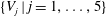 $\{V_{j}\mid j=1,\ldots ,5\}$
to vanish.
$\{V_{j}\mid j=1,\ldots ,5\}$
to vanish.
6 Characterization of the weakly compressible vortex streets
We set length and time scales with the choices
 $\unicode[STIX]{x1D6E4}=L=1$
. We define the street aspect ratio
$\unicode[STIX]{x1D6E4}=L=1$
. We define the street aspect ratio
 $\unicode[STIX]{x1D705}$
to be
$\unicode[STIX]{x1D705}$
to be
 $$\begin{eqnarray}\unicode[STIX]{x1D705}=\frac{h}{L},\end{eqnarray}$$
where
 $h$
denotes the vertical separation of the vortex centroids of the two vortices in each period window.
$h$
denotes the vertical separation of the vortex centroids of the two vortices in each period window.
The effect of vortex area on the speed of the street is shown in figure 2 for a selection of street aspect ratios. An important check on the foregoing analysis is provided by the small-area limit, where we expect the results here to tend to those given by an independent analysis of the weakly compressible point vortex streets recently calculated by Crowdy & Krishnamurthy (Reference Crowdy and Krishnamurthy2017), who find formula (1.1) for the first-order relative change in the speed of a staggered street. This is found to be the case. The values of
 $\unicode[STIX]{x0394}U/U$
predicted by (1.1) are indicated by solid dots on the vertical axis of figure 2. This reassures us that the numerical scheme described in previous sections is faithfully computing the finite-area continuations of the compressible point vortex result (1.1). Table 1 provides some typical parameter values obtained using our method.
$\unicode[STIX]{x0394}U/U$
predicted by (1.1) are indicated by solid dots on the vertical axis of figure 2. This reassures us that the numerical scheme described in previous sections is faithfully computing the finite-area continuations of the compressible point vortex result (1.1). Table 1 provides some typical parameter values obtained using our method.

Figure 2. Graph of the relative change in the speed of the vortex street
 $\unicode[STIX]{x0394}U/U$
against vortex area for fixed street aspect ratio
$\unicode[STIX]{x0394}U/U$
against vortex area for fixed street aspect ratio
 $\unicode[STIX]{x1D705}=0.2,0.28$
and
$\unicode[STIX]{x1D705}=0.2,0.28$
and
 $0.34$
. The dots on the vertical axis at zero area show the results of the analysis of the point vortex street of Crowdy & Krishnamurthy (Reference Crowdy and Krishnamurthy2017).
$0.34$
. The dots on the vertical axis at zero area show the results of the analysis of the point vortex street of Crowdy & Krishnamurthy (Reference Crowdy and Krishnamurthy2017).
Table 1. A representative table of parameters values for
 $\unicode[STIX]{x1D705}=0.28$
. For the given
$\unicode[STIX]{x1D705}=0.28$
. For the given
 $\unicode[STIX]{x1D70C}_{0}$
, the incompressible parameters
$\unicode[STIX]{x1D70C}_{0}$
, the incompressible parameters
 $\{\unicode[STIX]{x1D6FC}_{0},\unicode[STIX]{x1D6FD}_{0},\unicode[STIX]{x1D6FE}_{1},\unicode[STIX]{x1D6FE}_{2},U\}$
are found, using the prescription described in § 2. The parameters
$\{\unicode[STIX]{x1D6FC}_{0},\unicode[STIX]{x1D6FD}_{0},\unicode[STIX]{x1D6FE}_{1},\unicode[STIX]{x1D6FE}_{2},U\}$
are found, using the prescription described in § 2. The parameters
 $\{\unicode[STIX]{x1D70C}_{1},\unicode[STIX]{x1D6FC}_{1},\unicode[STIX]{x1D6FD}_{1},\unicode[STIX]{x0394}U\}$
associated with the first-order compressible correction are then calculated using the prescription described in § 5.
$\{\unicode[STIX]{x1D70C}_{1},\unicode[STIX]{x1D6FC}_{1},\unicode[STIX]{x1D6FD}_{1},\unicode[STIX]{x0394}U\}$
associated with the first-order compressible correction are then calculated using the prescription described in § 5.
We focus on aspect ratios around the value
 $0.28$
; this is close to the isolated value for neutral linear stability of the von Kármán point vortex streets, and it has been established (Jimenez Reference Jimenez1987) that the same isolated neutral stability point exists even for finite-area incompressible vortex street models with a Hamiltonian structure. Given these special stability features, to study the properties of steady compressible streets close to
$0.28$
; this is close to the isolated value for neutral linear stability of the von Kármán point vortex streets, and it has been established (Jimenez Reference Jimenez1987) that the same isolated neutral stability point exists even for finite-area incompressible vortex street models with a Hamiltonian structure. Given these special stability features, to study the properties of steady compressible streets close to
 $\unicode[STIX]{x1D705}=0.28$
would seem to be of particular interest (although it must be emphasized that we say nothing here on the stability of these compressible vortex equilibria). Moreover, as
$\unicode[STIX]{x1D705}=0.28$
would seem to be of particular interest (although it must be emphasized that we say nothing here on the stability of these compressible vortex equilibria). Moreover, as
 $\unicode[STIX]{x1D705}\rightarrow 0$
, the staggered street tends to an arrangement comprising a single periodic row of counter-rotating vortices. A study of compressibility effects on such a vortex configuration – albeit within a different model of the vortex cores – has already been carried out by O’Reilly & Pullin (Reference O’Reilly and Pullin2005), so we do not focus on it here.
$\unicode[STIX]{x1D705}\rightarrow 0$
, the staggered street tends to an arrangement comprising a single periodic row of counter-rotating vortices. A study of compressibility effects on such a vortex configuration – albeit within a different model of the vortex cores – has already been carried out by O’Reilly & Pullin (Reference O’Reilly and Pullin2005), so we do not focus on it here.
We find that compressibility tends to increase the speed of streets of small vortices but that there is a critical vortex area at which no change in the speed of the street at first order in
 $M^{2}$
occurs. For streets with vortices of area greater than this critical size, compressibility decreases the speed of the street.
$M^{2}$
occurs. For streets with vortices of area greater than this critical size, compressibility decreases the speed of the street.

Figure 3. Critical value of the normalized effective core radius
 $R_{c}/L$
as a function of
$R_{c}/L$
as a function of
 $\unicode[STIX]{x1D705}/2$
, at which
$\unicode[STIX]{x1D705}/2$
, at which
 $\unicode[STIX]{x0394}U=0$
, so that compressibility does not alter the speed of the street at first order in
$\unicode[STIX]{x0394}U=0$
, so that compressibility does not alter the speed of the street at first order in
 $M^{2}$
. The linear approximation (6.3) is also shown (dotted line).
$M^{2}$
. The linear approximation (6.3) is also shown (dotted line).
The presence of a critical vortex core size for which compressibility does not affect the street speed at first order in Mach number is interesting. For aspect ratio
 $\unicode[STIX]{x1D705}=0.28$
, we find the critical area to be
$\unicode[STIX]{x1D705}=0.28$
, we find the critical area to be
 $0.0655$
. The associated vortices are not circular but we can nevertheless infer an effective core radius
$0.0655$
. The associated vortices are not circular but we can nevertheless infer an effective core radius
 $R_{c}$
associated with this critical area by assuming a circular shape and setting
$R_{c}$
associated with this critical area by assuming a circular shape and setting
 $$\begin{eqnarray}\unicode[STIX]{x03C0}\left(\frac{R_{c}}{L}\right)^{2}=0.0665\quad \text{implying}~R_{c}\approx 0.14L.\end{eqnarray}$$
In this case, the normalized effective radius
 $R_{c}$
corresponds approximately to the vertical distance of each vortex from the centreline
$R_{c}$
corresponds approximately to the vertical distance of each vortex from the centreline
 $y=0$
of the two vortex rows, i.e.
$y=0$
of the two vortex rows, i.e.
 $\unicode[STIX]{x1D705}/2$
, for this aspect ratio. A graph of
$\unicode[STIX]{x1D705}/2$
, for this aspect ratio. A graph of
 $R_{c}/L$
against
$R_{c}/L$
against
 $\unicode[STIX]{x1D705}/2$
is shown in figure 3 and shows a near-linear behaviour closely approximated by
$\unicode[STIX]{x1D705}/2$
is shown in figure 3 and shows a near-linear behaviour closely approximated by
 $$\begin{eqnarray}\frac{R_{c}}{L}=0.22\left(\frac{\unicode[STIX]{x1D705}}{2}\right)+0.11,\end{eqnarray}$$
which may be useful in providing ready estimates of the critical vortex area at which vortices are unaffected by compressibility to leading order in
 $M^{2}$
.
$M^{2}$
.

Figure 4. Graph of the first-order relative change in the fluid speed on the vortex boundary
 $\unicode[STIX]{x0394}q/q_{0}$
against vortex area for fixed street aspect ratio
$\unicode[STIX]{x0394}q/q_{0}$
against vortex area for fixed street aspect ratio
 $\unicode[STIX]{x1D705}=0.2,0.28$
and
$\unicode[STIX]{x1D705}=0.2,0.28$
and
 $0.34$
.
$0.34$
.

Figure 5. Graph of the relative change in the speed of the vortex street
 $\unicode[STIX]{x0394}U/U$
against street aspect ratio
$\unicode[STIX]{x0394}U/U$
against street aspect ratio
 $\unicode[STIX]{x1D705}$
for fixed values of vortex area
$\unicode[STIX]{x1D705}$
for fixed values of vortex area
 $0.04,0.1$
and
$0.04,0.1$
and
 $0.2$
.
$0.2$
.

Figure 6. Effect of compressibility on the vortex shapes: (a) for
 $\unicode[STIX]{x1D705}=0.28$
and
$\unicode[STIX]{x1D705}=0.28$
and
 $\unicode[STIX]{x1D70C}=0.122$
, for which the vortex area is at its critical value
$\unicode[STIX]{x1D70C}=0.122$
, for which the vortex area is at its critical value
 $0.0654$
; and (b) for
$0.0654$
; and (b) for
 $\unicode[STIX]{x1D705}=0.2$
and
$\unicode[STIX]{x1D705}=0.2$
and
 $\unicode[STIX]{x1D70C}=0.5$
, for which the vortex area is
$\unicode[STIX]{x1D70C}=0.5$
, for which the vortex area is
 $0.2485$
. The incompressible vortices (dashed line) and the compressible analogues (solid line) having the same area are superposed. The value
$0.2485$
. The incompressible vortices (dashed line) and the compressible analogues (solid line) having the same area are superposed. The value
 $M^{2}=0.4$
is taken in order to exaggerate the qualitative difference in shapes for the compressible vortices.
$M^{2}=0.4$
is taken in order to exaggerate the qualitative difference in shapes for the compressible vortices.
Figure 4 shows the first-order relative change in the fluid speed on the boundary
 $\unicode[STIX]{x0394}q/q_{0}$
as a function of vortex area for the fixed street aspect ratios
$\unicode[STIX]{x0394}q/q_{0}$
as a function of vortex area for the fixed street aspect ratios
 $\unicode[STIX]{x1D705}=0.2,0.28$
and
$\unicode[STIX]{x1D705}=0.2,0.28$
and
 $0.34$
. It is found to be negative, which means, since the circulation of the vortices is fixed to be the same as in the incompressible case, that the perimeter of the perturbed compressible vortices increases relative to their incompressible counterparts.
$0.34$
. It is found to be negative, which means, since the circulation of the vortices is fixed to be the same as in the incompressible case, that the perimeter of the perturbed compressible vortices increases relative to their incompressible counterparts.
Figure 5 shows the first-order relative change in the speed of the street
 $\unicode[STIX]{x0394}U/U$
as a function of street aspect ratio for three fixed values of the vortex area
$\unicode[STIX]{x0394}U/U$
as a function of street aspect ratio for three fixed values of the vortex area
 $0.04,0.1$
and
$0.04,0.1$
and
 $0.2$
. A notable feature of both figures 2 and 5 is that, as the aspect ratio of the street decreases towards zero, the magnitude of the first-order relative change in the compressible speed becomes large. This singular-looking behaviour is to be expected, however, since, as pointed out earlier, our choice of Mach number based on the speed of translation of the incompressible street tends to zero as
$0.2$
. A notable feature of both figures 2 and 5 is that, as the aspect ratio of the street decreases towards zero, the magnitude of the first-order relative change in the compressible speed becomes large. This singular-looking behaviour is to be expected, however, since, as pointed out earlier, our choice of Mach number based on the speed of translation of the incompressible street tends to zero as
 $\unicode[STIX]{x1D705}\rightarrow 0$
(that is, our choice of expansion parameter
$\unicode[STIX]{x1D705}\rightarrow 0$
(that is, our choice of expansion parameter
 $M$
is tending to zero). A vortex street with
$M$
is tending to zero). A vortex street with
 $\unicode[STIX]{x1D705}=0$
reduces to the situation of a single row of vortices of alternating sign and this arrangement is not of particular interest to us here given our focus on vortex wakes. A Rayleigh–Jansen analysis of this scenario would require a different choice of Mach number as the expansion parameter.
$\unicode[STIX]{x1D705}=0$
reduces to the situation of a single row of vortices of alternating sign and this arrangement is not of particular interest to us here given our focus on vortex wakes. A Rayleigh–Jansen analysis of this scenario would require a different choice of Mach number as the expansion parameter.
Figure 5 shows that the relative change in speed of the street due to compressibility tends to zero as
 $\unicode[STIX]{x1D705}$
increases in all cases. For vortex area
$\unicode[STIX]{x1D705}$
increases in all cases. For vortex area
 $0.04$
, the relative change in compressible street speed is around 7 % for
$0.04$
, the relative change in compressible street speed is around 7 % for
 $\unicode[STIX]{x1D705}=0.28$
and it gets smaller as
$\unicode[STIX]{x1D705}=0.28$
and it gets smaller as
 $\unicode[STIX]{x1D705}$
increases further.
$\unicode[STIX]{x1D705}$
increases further.
Finally, we document the effect of compressibility on the vortex shapes, and this is represented in figure 6 for two choices of vortex street of different aspect ratio and vortex areas. The same qualitative trend appears to be true in all cases: compressibility leads to an elongation of the vortices in the cross-stream direction, with the vortices becoming more slender in the streamwise direction. These effects become more pronounced, for a given Mach number, for vortices of larger area, as shown in figure 6. As already pointed out with reference to figure 4, the perimeter of the perturbed vortices generally increases at first order in
 $M^{2}$
relative to the incompressible counterparts of the same area, circulation and aspect ratio. These observations on the shape deformations due to weak compressibility are consistent with analogous observations made by O’Reilly & Pullin (Reference O’Reilly and Pullin2005) in their numerical examination of the compressible analogues of the smooth counter-rotating vortex pair found by Mallier & Maslowe (Reference Mallier and Maslowe1993). O’Reilly & Pullin (Reference O’Reilly and Pullin2005) noticed that compressibility acts to increase the strain rates in the smooth vortex cores, causing substantial stretching of the vortices in the transverse direction to the axis of the vortex row.
$M^{2}$
relative to the incompressible counterparts of the same area, circulation and aspect ratio. These observations on the shape deformations due to weak compressibility are consistent with analogous observations made by O’Reilly & Pullin (Reference O’Reilly and Pullin2005) in their numerical examination of the compressible analogues of the smooth counter-rotating vortex pair found by Mallier & Maslowe (Reference Mallier and Maslowe1993). O’Reilly & Pullin (Reference O’Reilly and Pullin2005) noticed that compressibility acts to increase the strain rates in the smooth vortex cores, causing substantial stretching of the vortices in the transverse direction to the axis of the vortex row.
7 Discussion
A small-Mach-number expansion about the incompressible staggered streets of hollow vortices found by Crowdy & Green (Reference Crowdy and Green2011) has been carried out. The results are given in quasi-analytical form, stated in the form of the solutions of modified Schwarz problems in a concentric annulus, with the boundary data conveniently expressed using a calculus based on the Schottky–Klein prime function of that annulus. The results should be straightforward to reproduce from the prescription set out here. It should be emphasized that, while we have chosen to fix both the area and centroid of the vortices, this is an arbitrary choice, and other choices are easily incorporated by altering the conditions (5.66). Those alternative choices might arise, say, by matching conditions if this Rayleigh–Jansen solution is embedded in some more general asymptotic analysis of a wave-like problem (Leppington Reference Leppington2006), or from some other physical stipulations.
Our main result is that, for a fixed street aspect ratio and fixed circulation of the vortices, the size of the vortices making up the street is critical in determining whether small-Mach-number effects increase or decrease the speed of the street relative to an incompressible street with the same parameters. Streets of vortices smaller than a critical area (which is a function of street aspect ratio) travel faster than an incompressible street with the same circulation and aspect ratio, while compressible streets comprising vortices larger than the critical value, with the same aspect ratio, travel more slowly relative to their incompressible counterpart.
A Rayleigh–Jansen expansion about the streets of vortex patches found by Saffman & Schatzman (Reference Saffman and Schatzman1981) has not yet been carried out, but it would be an interesting exercise. It is more challenging than the hollow vortex problem considered here because of both the need to resolve the internal structure of the vortex core, and the lack of any known analytical solution for the incompressible solutions. The core structure details do not matter for small-area vortices (Crowdy & Krishnamurthy Reference Crowdy and Krishnamurthy2017), but how the core structure affects the results obtained here as the vortex cores grow in size is of theoretical interest. The effect of vortex core structure on the speed of thin-cored vortex rings has been well studied theoretically (Moore Reference Moore1985; Saffman Reference Saffman1992), and similar detailed studies of vortex streets are desirable.
Our results may have implications in understanding both the structure, and evolution, of compressible wakes, or the scattering or generation of sound waves from wake structures. It would be an interesting challenge to explore whether a model for compressible wakes built on the solutions here can be formulated following in the spirit of a similar model (Saffman & Schatzman Reference Saffman and Schatzman1982a ) for incompressible wakes built on the incompressible vortex patch wakes computed numerically by the same authors (Saffman & Schatzman Reference Saffman and Schatzman1981, Reference Saffman and Schatzman1982b ). Saffman & Schatzman (Reference Saffman and Schatzman1982a ) use curve fits to the detailed numerical calculations of Saffman & Schatzman (Reference Saffman and Schatzman1981) to feed into their wake models, and a similar strategy could in principle be adopted using the results of this paper if a generalized weakly compressible wake model was to be formulated.
A pressing matter, yet to be examined, is the question of the stability properties of the steady weakly compressible vortex streets found here. This is a challenging task, and is left for a future investigation. There is much active research in trying to understand the effects of compressibility on the structural evolution of transitional high-speed planar wakes, with recent work (Hickey, Hussain & Wu Reference Hickey, Hussain and Wu2016) indicating that quasi-two-dimensional planar wakes of the kind examined here have a role to play. The significance of the results herein to such studies has yet to be ascertained. Even the linear stability properties of the incompressible vortex streets of Crowdy & Green (Reference Crowdy and Green2011) have yet to be computed; indeed, it is only recently that the linear stability properties of the incompressible hollow vortex pair solutions found by Pocklington (Reference Pocklington1895) were worked out (Crowdy, Llewellyn Smith & Freilich Reference Crowdy, Llewellyn Smith and Freilich2012). The fact that the work here gives an analytical handle on the steady compressible solutions, at least for small Mach numbers, should be of great help in facilitating a study of their linear stability.
The formulation for compressible hollow vortex flows given here can be adapted to a numerical investigation at larger Mach numbers. The numerical scheme of Moore & Pullin (Reference Moore and Pullin1987), which uses a change of independent variables to a hodograph plane, requires certain a priori assumptions on the solutions (in particular, it is unable to capture classes of solution which potentially form what those authors call a ‘waist’ in the hodograph plane). A numerical formulation based on the conformal mapping description of the two vortices advocated here would not be limited in the same way. The small-Mach-number results here can be used as a numerical check on any such numerical formulation, and as a seed for a nonlinear numerical continuation scheme as the Mach number is increased.
A simple extension of this study would be to assume that the vortices contain a second compressible barotropic gas, of uniform pressure, but with a simple relation between the enclosed gas pressure and the vortex area. Another extension is to include surface tension: one of the authors has previously found analytical solutions for isolated hollow vortices with surface tension effects active on the vortex boundary (Crowdy Reference Crowdy1999). Those incompressible solutions were also found using conformal mappings from the unit disc, so a generalization of the weakly compressible analysis herein should facilitate a Rayleigh–Jansen expansion of those solutions too.
Acknowledgements
The authors thank S. Llewellyn Smith for many helpful discussions. D.G.C. (orcid.org/0000-0002-7162-0181) is supported by an EPSRC Established Career Fellowship (EP/K019430/10) and a Royal Society Wolfson Research Merit Award. V.S.K. (orcid.org/0000-0002-1518-0994) acknowledges financial support from a Rector’s Scholarship from Imperial College London with additional support from the Department of Mathematics there.
Supplementary material
Supplementary material is available at https://doi.org/10.1017/jfm.2017.821.
Appendix A. The Schottky–Klein prime function
We make extended use of properties of the special function defined by
 $$\begin{eqnarray}P(\unicode[STIX]{x1D701},\unicode[STIX]{x1D70C}_{0})=(1-\unicode[STIX]{x1D701})\mathop{\prod }_{k=1}^{\infty }(1-\unicode[STIX]{x1D70C}_{0}^{2k}\unicode[STIX]{x1D701})(1-\unicode[STIX]{x1D70C}_{0}^{2k}\unicode[STIX]{x1D701}^{-1}),\end{eqnarray}$$
together with its derivatives. This function is, to within a normalization, the Schottky–Klein prime function (Crowdy Reference Crowdy2008a
, Reference Crowdy2010) of the annulus
 $\unicode[STIX]{x1D70C}_{0}<|\unicode[STIX]{x1D701}|<1$
. It is helpful to record some of its basic properties. It is apparent from (A 1) that
$\unicode[STIX]{x1D70C}_{0}<|\unicode[STIX]{x1D701}|<1$
. It is helpful to record some of its basic properties. It is apparent from (A 1) that
 $P(\unicode[STIX]{x1D701},\unicode[STIX]{x1D70C}_{0})$
has a simple zero at
$P(\unicode[STIX]{x1D701},\unicode[STIX]{x1D70C}_{0})$
has a simple zero at
 $\unicode[STIX]{x1D701}=1$
. It is easy to show, directly from the infinite product definition (A 1), that
$\unicode[STIX]{x1D701}=1$
. It is easy to show, directly from the infinite product definition (A 1), that
 $$\begin{eqnarray}P(\unicode[STIX]{x1D70C}_{0}^{2}\unicode[STIX]{x1D701},\unicode[STIX]{x1D70C}_{0})=-\unicode[STIX]{x1D701}^{-1}P(\unicode[STIX]{x1D701},\unicode[STIX]{x1D70C}_{0}),\quad P(\unicode[STIX]{x1D701}^{-1},\unicode[STIX]{x1D70C}_{0})=-\unicode[STIX]{x1D701}^{-1}P(\unicode[STIX]{x1D701},\unicode[STIX]{x1D70C}_{0}).\end{eqnarray}$$
We also introduce
 $$\begin{eqnarray}K(\unicode[STIX]{x1D701},\unicode[STIX]{x1D70C}_{0})={\displaystyle \frac{\unicode[STIX]{x1D701}}{P(\unicode[STIX]{x1D701},\unicode[STIX]{x1D70C}_{0})}}\frac{\unicode[STIX]{x2202}P(\unicode[STIX]{x1D701},\unicode[STIX]{x1D70C}_{0})}{\unicode[STIX]{x2202}\unicode[STIX]{x1D701}}.\end{eqnarray}$$
This function can be represented by the infinite sum
 $$\begin{eqnarray}K(\unicode[STIX]{x1D701},\unicode[STIX]{x1D70C}_{0})=-{\displaystyle \frac{\unicode[STIX]{x1D701}}{1-\unicode[STIX]{x1D701}}}-\mathop{\sum }_{k=1}^{\infty }{\displaystyle \frac{\unicode[STIX]{x1D70C}_{0}^{2k}\unicode[STIX]{x1D701}}{1-\unicode[STIX]{x1D70C}_{0}^{2k}\unicode[STIX]{x1D701}}}+\mathop{\sum }_{k=1}^{\infty }{\displaystyle \frac{\unicode[STIX]{x1D70C}_{0}^{2k}\unicode[STIX]{x1D701}^{-1}}{1-\unicode[STIX]{x1D70C}_{0}^{2k}\unicode[STIX]{x1D701}^{-1}}}.\end{eqnarray}$$
It can be shown from (A 2) that
 $$\begin{eqnarray}K(\unicode[STIX]{x1D70C}_{0}^{2}\unicode[STIX]{x1D701},\unicode[STIX]{x1D70C}_{0})=K(\unicode[STIX]{x1D701},\unicode[STIX]{x1D70C}_{0})-1,\quad K(1/\unicode[STIX]{x1D701},\unicode[STIX]{x1D70C}_{0})=1-K(\unicode[STIX]{x1D701},\unicode[STIX]{x1D70C}_{0}).\end{eqnarray}$$
It is also worth noting that, near
 $\unicode[STIX]{x1D701}=1$
,
$\unicode[STIX]{x1D701}=1$
,
 $$\begin{eqnarray}K(\unicode[STIX]{x1D701},\unicode[STIX]{x1D70C}_{0})\sim {\displaystyle \frac{1}{\unicode[STIX]{x1D701}-1}}+\text{locally analytic function},\end{eqnarray}$$
so it has a simple pole there.
Appendix B. Derivation of the new form of
$z_{0}(\unicode[STIX]{x1D701})$

Crowdy & Green (Reference Crowdy and Green2011) present the solution (2.3) and (2.4) as follows:
 $$\begin{eqnarray}\left.\begin{array}{@{}c@{}}f=f_{0}(\unicode[STIX]{x1D701})=\frac{\displaystyle \text{i}LU}{\displaystyle 2\unicode[STIX]{x03C0}}\log \left[\frac{\displaystyle |\unicode[STIX]{x1D6FC}_{0}|P(\unicode[STIX]{x1D701}/\unicode[STIX]{x1D6FC}_{0},\unicode[STIX]{x1D70C}_{0})P(\unicode[STIX]{x1D701}\unicode[STIX]{x1D6FD}_{0},\unicode[STIX]{x1D70C}_{0})}{\displaystyle |\unicode[STIX]{x1D6FD}_{0}|P(\unicode[STIX]{x1D701}\unicode[STIX]{x1D6FC}_{0},\unicode[STIX]{x1D70C}_{0})P(\unicode[STIX]{x1D701}/\unicode[STIX]{x1D6FD}_{0},\unicode[STIX]{x1D70C}_{0})}\right]-\frac{\displaystyle \text{i}\unicode[STIX]{x1D6E4}}{\displaystyle 2\unicode[STIX]{x03C0}}\log \unicode[STIX]{x1D701},\\ z=z_{0}(\unicode[STIX]{x1D701})=\displaystyle \int ^{\unicode[STIX]{x1D701}}\left\{\frac{\displaystyle BP^{2}(\unicode[STIX]{x1D701}^{\prime }\overline{\unicode[STIX]{x1D6FE}_{1}},\unicode[STIX]{x1D70C}_{0})P^{2}(\unicode[STIX]{x1D701}^{\prime }\overline{\unicode[STIX]{x1D6FE}_{2}},\unicode[STIX]{x1D70C}_{0})}{\displaystyle P(\unicode[STIX]{x1D701}^{\prime }/\unicode[STIX]{x1D6FC}_{0},\unicode[STIX]{x1D70C}_{0})P(\unicode[STIX]{x1D701}^{\prime }\overline{\unicode[STIX]{x1D6FC}_{0}},\unicode[STIX]{x1D70C}_{0})P(\unicode[STIX]{x1D701}^{\prime }/\unicode[STIX]{x1D6FD}_{0},\unicode[STIX]{x1D70C}_{0})P(\unicode[STIX]{x1D701}^{\prime }\overline{\unicode[STIX]{x1D6FD}_{0}},\unicode[STIX]{x1D70C}_{0})}\right\}\text{d}\unicode[STIX]{x1D701}^{\prime },\end{array}\right\}\end{eqnarray}$$
where the representation for
 $z_{0}(\unicode[STIX]{x1D701})$
differs from, but is equivalent to, that given in (2.4). We now show why this is true. The conformal mapping (B 1) implies
$z_{0}(\unicode[STIX]{x1D701})$
differs from, but is equivalent to, that given in (2.4). We now show why this is true. The conformal mapping (B 1) implies
 $$\begin{eqnarray}z_{0}^{\prime }(\unicode[STIX]{x1D701})=\frac{{\mathcal{Q}}(\unicode[STIX]{x1D701})}{\unicode[STIX]{x1D701}},\end{eqnarray}$$
where
 $$\begin{eqnarray}{\mathcal{Q}}(\unicode[STIX]{x1D701})\equiv \frac{B\unicode[STIX]{x1D701}P^{2}(\unicode[STIX]{x1D701}\overline{\unicode[STIX]{x1D6FE}_{1}},\unicode[STIX]{x1D70C}_{0})P^{2}(\unicode[STIX]{x1D701}\overline{\unicode[STIX]{x1D6FE}_{2}},\unicode[STIX]{x1D70C}_{0})}{P(\unicode[STIX]{x1D701}/\unicode[STIX]{x1D6FC}_{0},\unicode[STIX]{x1D70C}_{0})P(\unicode[STIX]{x1D701}\unicode[STIX]{x1D6FC}_{0},\unicode[STIX]{x1D70C}_{0})P(\unicode[STIX]{x1D701}/\unicode[STIX]{x1D6FD}_{0},\unicode[STIX]{x1D70C}_{0})P(\unicode[STIX]{x1D701}\unicode[STIX]{x1D6FD}_{0},\unicode[STIX]{x1D70C}_{0})}.\end{eqnarray}$$
It can be verified, on use of the properties of the function
 $P(\unicode[STIX]{x1D701},\unicode[STIX]{x1D70C}_{0})$
summarized in appendix A, that
$P(\unicode[STIX]{x1D701},\unicode[STIX]{x1D70C}_{0})$
summarized in appendix A, that
 $$\begin{eqnarray}{\mathcal{Q}}(\unicode[STIX]{x1D70C}_{0}^{2}\unicode[STIX]{x1D701})={\mathcal{Q}}(\unicode[STIX]{x1D701}).\end{eqnarray}$$
Since
 ${\mathcal{Q}}(\unicode[STIX]{x1D701})$
is meromorphic, and satisfies the functional identity (B 4), it is called a loxodromic function (Crowdy Reference Crowdy2008a
). We can therefore write
${\mathcal{Q}}(\unicode[STIX]{x1D701})$
is meromorphic, and satisfies the functional identity (B 4), it is called a loxodromic function (Crowdy Reference Crowdy2008a
). We can therefore write
 $$\begin{eqnarray}{\mathcal{Q}}(\unicode[STIX]{x1D701})=aK(\unicode[STIX]{x1D701}/\unicode[STIX]{x1D6FC}_{0},\unicode[STIX]{x1D70C}_{0})+bK(\unicode[STIX]{x1D701}\unicode[STIX]{x1D6FC}_{0},\unicode[STIX]{x1D70C}_{0})+cK(\unicode[STIX]{x1D701}/\unicode[STIX]{x1D6FD}_{0},\unicode[STIX]{x1D70C}_{0})+\text{d}K(\unicode[STIX]{x1D701}\unicode[STIX]{x1D6FD}_{0},\unicode[STIX]{x1D70C}_{0})+e,\end{eqnarray}$$
for some constants
 $a,b,c,d$
and
$a,b,c,d$
and
 $e$
, which must satisfy
$e$
, which must satisfy
 $$\begin{eqnarray}a+b+c+d=0.\end{eqnarray}$$
The latter condition is required in order that
 ${\mathcal{Q}}(\unicode[STIX]{x1D701})$
satisfies (B 4), a fact that follows on use of the properties of the function
${\mathcal{Q}}(\unicode[STIX]{x1D701})$
satisfies (B 4), a fact that follows on use of the properties of the function
 $K(\unicode[STIX]{x1D701},\unicode[STIX]{x1D70C}_{0})$
(see appendix A). We therefore have two expressions, equations (B 3) and (B 5), for the same loxodromic function, this equivalence being akin to a partial fraction decomposition of a rational function. By equating the strengths of the poles at
$K(\unicode[STIX]{x1D701},\unicode[STIX]{x1D70C}_{0})$
(see appendix A). We therefore have two expressions, equations (B 3) and (B 5), for the same loxodromic function, this equivalence being akin to a partial fraction decomposition of a rational function. By equating the strengths of the poles at
 $\unicode[STIX]{x1D701}=\unicode[STIX]{x1D6FC}_{0}$
and
$\unicode[STIX]{x1D701}=\unicode[STIX]{x1D6FC}_{0}$
and
 $\unicode[STIX]{x1D701}=\unicode[STIX]{x1D6FD}_{0}$
, we find, respectively,
$\unicode[STIX]{x1D701}=\unicode[STIX]{x1D6FD}_{0}$
, we find, respectively,
 $$\begin{eqnarray}a=-\frac{BP^{2}(\unicode[STIX]{x1D6FC}_{0}\overline{\unicode[STIX]{x1D6FE}_{1}},\unicode[STIX]{x1D70C}_{0})P^{2}(\unicode[STIX]{x1D6FC}_{0}\overline{\unicode[STIX]{x1D6FE}_{2}},\unicode[STIX]{x1D70C}_{0})}{\hat{P}(1,\unicode[STIX]{x1D70C}_{0})P(\unicode[STIX]{x1D6FC}_{0}^{2},\unicode[STIX]{x1D70C}_{0})P(\unicode[STIX]{x1D6FC}_{0}/\unicode[STIX]{x1D6FD}_{0},\unicode[STIX]{x1D70C}_{0})P(\unicode[STIX]{x1D6FC}_{0}\unicode[STIX]{x1D6FD}_{0},\unicode[STIX]{x1D70C}_{0})}\end{eqnarray}$$
and
 $$\begin{eqnarray}c=-\frac{BP^{2}(\unicode[STIX]{x1D6FD}_{0}\overline{\unicode[STIX]{x1D6FE}_{1}},\unicode[STIX]{x1D70C}_{0})P^{2}(\unicode[STIX]{x1D6FD}_{0}\overline{\unicode[STIX]{x1D6FE}_{2}},\unicode[STIX]{x1D70C}_{0})}{\hat{P}(1,\unicode[STIX]{x1D70C}_{0})P(\unicode[STIX]{x1D6FD}_{0}^{2},\unicode[STIX]{x1D70C}_{0})P(\unicode[STIX]{x1D6FD}_{0}/\unicode[STIX]{x1D6FC}_{0},\unicode[STIX]{x1D70C}_{0})P(\unicode[STIX]{x1D6FC}_{0}\unicode[STIX]{x1D6FD}_{0},\unicode[STIX]{x1D70C}_{0})}.\end{eqnarray}$$
But on use of (2.7),
 $$\begin{eqnarray}P(\unicode[STIX]{x1D6FD}_{0}^{2},\unicode[STIX]{x1D70C}_{0})=P(\unicode[STIX]{x1D6FC}_{0}^{2},\unicode[STIX]{x1D70C}_{0}),\quad P(\unicode[STIX]{x1D6FD}_{0}\overline{\unicode[STIX]{x1D6FE}_{1}},\unicode[STIX]{x1D70C}_{0})=P(\unicode[STIX]{x1D6FC}_{0}\overline{\unicode[STIX]{x1D6FE}_{2}},\unicode[STIX]{x1D70C}_{0}),\end{eqnarray}$$
which can be used to show that
 $$\begin{eqnarray}c=-a.\end{eqnarray}$$
By equating the strength of the pole at
 $\unicode[STIX]{x1D701}=1/\unicode[STIX]{x1D6FC}_{0}$
, we find
$\unicode[STIX]{x1D701}=1/\unicode[STIX]{x1D6FC}_{0}$
, we find
 $$\begin{eqnarray}b=-\frac{BP^{2}(\overline{\unicode[STIX]{x1D6FE}_{1}}/\unicode[STIX]{x1D6FC}_{0},\unicode[STIX]{x1D70C}_{0})P^{2}(\overline{\unicode[STIX]{x1D6FE}_{2}}/\unicode[STIX]{x1D6FC}_{0},\unicode[STIX]{x1D70C}_{0})}{\unicode[STIX]{x1D6FC}_{0}\hat{P}(1,\unicode[STIX]{x1D70C}_{0})P(1/\unicode[STIX]{x1D6FC}_{0}^{2},\unicode[STIX]{x1D70C}_{0})P(1/\unicode[STIX]{x1D6FC}_{0}\unicode[STIX]{x1D6FD}_{0},\unicode[STIX]{x1D70C}_{0})P(\unicode[STIX]{x1D6FD}_{0}/\unicode[STIX]{x1D6FC}_{0},\unicode[STIX]{x1D70C}_{0})}.\end{eqnarray}$$
Some calculations using the properties of
 $P(\unicode[STIX]{x1D701},\unicode[STIX]{x1D70C}_{0})$
lead to the deduction that
$P(\unicode[STIX]{x1D701},\unicode[STIX]{x1D70C}_{0})$
lead to the deduction that
 $$\begin{eqnarray}b=-\unicode[STIX]{x1D712}a,\end{eqnarray}$$
where
 $\unicode[STIX]{x1D712}$
is defined in (2.6). It then follows from (B 6) that
$\unicode[STIX]{x1D712}$
is defined in (2.6). It then follows from (B 6) that
 $$\begin{eqnarray}d=\unicode[STIX]{x1D712}a.\end{eqnarray}$$
In order that
 $z_{0}(\unicode[STIX]{x1D701})$
is single-valued around the circles
$z_{0}(\unicode[STIX]{x1D701})$
is single-valued around the circles
 $|\unicode[STIX]{x1D701}|=\unicode[STIX]{x1D70C}_{0},1$
– so that the image of these circles under the mapping function forms closed curves – we need to set
$|\unicode[STIX]{x1D701}|=\unicode[STIX]{x1D70C}_{0},1$
– so that the image of these circles under the mapping function forms closed curves – we need to set
 $$\begin{eqnarray}e=0.\end{eqnarray}$$
This is one condition to determine the unknown parameters. Crowdy & Green (Reference Crowdy and Green2011) enforce the same condition based on their indefinite integral representation (B 1). Now
 $z_{0}^{\prime }(\unicode[STIX]{x1D701})$
, and hence
$z_{0}^{\prime }(\unicode[STIX]{x1D701})$
, and hence
 ${\mathcal{Q}}(\unicode[STIX]{x1D701})$
, must vanish at
${\mathcal{Q}}(\unicode[STIX]{x1D701})$
, must vanish at
 $1/\unicode[STIX]{x1D6FE}_{1}$
and
$1/\unicode[STIX]{x1D6FE}_{1}$
and
 $1/\unicode[STIX]{x1D6FE}_{2}$
, implying, for instance, that
$1/\unicode[STIX]{x1D6FE}_{2}$
, implying, for instance, that
 $$\begin{eqnarray}0=a[K(1/(\unicode[STIX]{x1D6FE}_{1}\unicode[STIX]{x1D6FC}_{0}),\unicode[STIX]{x1D70C}_{0})-\unicode[STIX]{x1D712}K(\unicode[STIX]{x1D6FC}_{0}/\unicode[STIX]{x1D6FE}_{1},\unicode[STIX]{x1D70C}_{0})-K(1/(\unicode[STIX]{x1D6FE}_{1}\unicode[STIX]{x1D6FD}_{0}),\unicode[STIX]{x1D70C}_{0})+\unicode[STIX]{x1D712}K(\unicode[STIX]{x1D6FD}_{0}/\unicode[STIX]{x1D6FE}_{1},\unicode[STIX]{x1D70C}_{0})]+e,\end{eqnarray}$$
which gives an equation for
 $e$
(a similar equation obtained from the other zero at
$e$
(a similar equation obtained from the other zero at
 $1/\unicode[STIX]{x1D6FE}_{2}$
gives the same result for
$1/\unicode[STIX]{x1D6FE}_{2}$
gives the same result for
 $e$
). Setting
$e$
). Setting
 $e=0$
yields
$e=0$
yields
 $$\begin{eqnarray}-K(\unicode[STIX]{x1D6FE}_{1}\unicode[STIX]{x1D6FC}_{0},\unicode[STIX]{x1D70C}_{0})-\unicode[STIX]{x1D712}K(\unicode[STIX]{x1D6FC}_{0}/\unicode[STIX]{x1D6FE}_{1},\unicode[STIX]{x1D70C}_{0})+K(\unicode[STIX]{x1D6FE}_{1}\unicode[STIX]{x1D6FD}_{0},\unicode[STIX]{x1D70C}_{0})+\unicode[STIX]{x1D712}K(\unicode[STIX]{x1D6FD}_{0}/\unicode[STIX]{x1D6FE}_{1},\unicode[STIX]{x1D70C}_{0})=0,\end{eqnarray}$$
where we have used (A 5b ). Also, we know from geometrical requirements on the mapping that
 $$\begin{eqnarray}z_{0}^{\prime }(\unicode[STIX]{x1D701})\sim -\frac{\text{i}L}{2\unicode[STIX]{x03C0}}\frac{1}{\unicode[STIX]{x1D701}-\unicode[STIX]{x1D6FC}_{0}},\quad \text{as }\unicode[STIX]{x1D701}\rightarrow \unicode[STIX]{x1D6FC}_{0}.\end{eqnarray}$$
Hence we arrive at the expression for
 $z_{0}(\unicode[STIX]{x1D701})$
given in (2.4).
$z_{0}(\unicode[STIX]{x1D701})$
given in (2.4).
Appendix C. Derivation of
${\mathcal{I}}(\unicode[STIX]{x1D701})$

The formula (5.12) can be derived using very similar arguments to those of appendix B. From Crowdy & Green (Reference Crowdy and Green2011) we know that
 $$\begin{eqnarray}\unicode[STIX]{x1D709}_{0}=\frac{\text{d}f_{0}}{\text{d}z}=\frac{f_{0}^{\prime }(\unicode[STIX]{x1D701})}{z_{0}^{\prime }(\unicode[STIX]{x1D701})}=\frac{R\unicode[STIX]{x1D702}(\unicode[STIX]{x1D701};\unicode[STIX]{x1D6FE}_{1})\unicode[STIX]{x1D702}(\unicode[STIX]{x1D701};\unicode[STIX]{x1D6FE}_{2})}{\unicode[STIX]{x1D701}},\quad \unicode[STIX]{x1D702}(\unicode[STIX]{x1D701},\unicode[STIX]{x1D6FE})=\frac{|\unicode[STIX]{x1D6FE}|P(\unicode[STIX]{x1D701}/\unicode[STIX]{x1D6FE},\unicode[STIX]{x1D70C}_{0})}{P(\unicode[STIX]{x1D701}\overline{\unicode[STIX]{x1D6FE}},\unicode[STIX]{x1D70C}_{0})},\end{eqnarray}$$
where we have rewritten the results of Crowdy & Green (Reference Crowdy and Green2011) in the present notation. It was also argued there (Crowdy & Green Reference Crowdy and Green2011) that
 $$\begin{eqnarray}\unicode[STIX]{x1D701}\frac{\text{d}f_{0}}{\text{d}\unicode[STIX]{x1D701}}=\frac{\tilde{R}P(\unicode[STIX]{x1D701}/\unicode[STIX]{x1D6FE}_{1},\unicode[STIX]{x1D70C}_{0})P(\unicode[STIX]{x1D701}\overline{\unicode[STIX]{x1D6FE}_{1}},\unicode[STIX]{x1D70C}_{0})P(\unicode[STIX]{x1D701}/\unicode[STIX]{x1D6FE}_{2},\unicode[STIX]{x1D70C}_{0})P(\unicode[STIX]{x1D701}\overline{\unicode[STIX]{x1D6FE}_{2}},\unicode[STIX]{x1D70C}_{0})}{P(\unicode[STIX]{x1D701}/\unicode[STIX]{x1D6FC}_{0},\unicode[STIX]{x1D70C}_{0})P(\unicode[STIX]{x1D701}\overline{\unicode[STIX]{x1D6FC}_{0}},\unicode[STIX]{x1D70C}_{0})P(\unicode[STIX]{x1D701}/\unicode[STIX]{x1D6FD}_{0},\unicode[STIX]{x1D70C}_{0})P(\unicode[STIX]{x1D701}\overline{\unicode[STIX]{x1D6FD}_{0}},\unicode[STIX]{x1D70C}_{0})},\end{eqnarray}$$
where
 $\tilde{R}$
is some complex constant. On combining (C 1) and (C 2), the integrand appearing in
$\tilde{R}$
is some complex constant. On combining (C 1) and (C 2), the integrand appearing in
 ${\mathcal{I}}(\unicode[STIX]{x1D701})$
is
${\mathcal{I}}(\unicode[STIX]{x1D701})$
is
 $$\begin{eqnarray}\frac{f_{0}^{\prime }(\unicode[STIX]{x1D701})^{2}}{z_{0}^{\prime }(\unicode[STIX]{x1D701})}=\frac{S}{\unicode[STIX]{x1D701}^{2}}\frac{P(\unicode[STIX]{x1D701}/\unicode[STIX]{x1D6FE}_{1},\unicode[STIX]{x1D70C}_{0})^{2}P(\unicode[STIX]{x1D701}/\unicode[STIX]{x1D6FE}_{2},\unicode[STIX]{x1D70C}_{0})^{2}}{P(\unicode[STIX]{x1D701}/\unicode[STIX]{x1D6FC}_{0},\unicode[STIX]{x1D70C}_{0})P(\unicode[STIX]{x1D701}\overline{\unicode[STIX]{x1D6FC}_{0}},\unicode[STIX]{x1D70C}_{0})P(\unicode[STIX]{x1D701}/\unicode[STIX]{x1D6FD}_{0},\unicode[STIX]{x1D70C}_{0})P(\unicode[STIX]{x1D701}\overline{\unicode[STIX]{x1D6FD}_{0}},\unicode[STIX]{x1D70C}_{0})},\end{eqnarray}$$
where
 $S$
is some constant. Consider now the subsidiary function
$S$
is some constant. Consider now the subsidiary function
 $$\begin{eqnarray}Q(\unicode[STIX]{x1D701})\equiv \frac{1}{\unicode[STIX]{x1D701}}\frac{P(\unicode[STIX]{x1D701}/\unicode[STIX]{x1D6FE}_{1},\unicode[STIX]{x1D70C}_{0})^{2}P(\unicode[STIX]{x1D701}/\unicode[STIX]{x1D6FE}_{2},\unicode[STIX]{x1D70C}_{0})^{2}}{P(\unicode[STIX]{x1D701}/\unicode[STIX]{x1D6FC}_{0},\unicode[STIX]{x1D70C}_{0})P(\unicode[STIX]{x1D701}\overline{\unicode[STIX]{x1D6FC}_{0}},\unicode[STIX]{x1D70C}_{0})P(\unicode[STIX]{x1D701}/\unicode[STIX]{x1D6FD}_{0},\unicode[STIX]{x1D70C}_{0})P(\unicode[STIX]{x1D701}\overline{\unicode[STIX]{x1D6FD}_{0}},\unicode[STIX]{x1D70C}_{0})}.\end{eqnarray}$$
The properties of
 $P(\unicode[STIX]{x1D701},\unicode[STIX]{x1D70C}_{0})$
, together with use of (2.7), can be used to show that
$P(\unicode[STIX]{x1D701},\unicode[STIX]{x1D70C}_{0})$
, together with use of (2.7), can be used to show that
 $$\begin{eqnarray}Q(\unicode[STIX]{x1D70C}_{0}^{2}\unicode[STIX]{x1D701})=Q(\unicode[STIX]{x1D701}),\end{eqnarray}$$
so that
 $Q(\unicode[STIX]{x1D701})$
is a loxodromic function. It should now be clear that manipulations entirely analogous to those given for
$Q(\unicode[STIX]{x1D701})$
is a loxodromic function. It should now be clear that manipulations entirely analogous to those given for
 $z_{0}(\unicode[STIX]{x1D701})$
in appendix B can be used to deduce (5.12).
$z_{0}(\unicode[STIX]{x1D701})$
in appendix B can be used to deduce (5.12).
Appendix D. Modified Schwarz problem in an annulus
Finding the two analytic functions appearing in the first-order correction of the complex potential and the conformal mapping requires the solution of several modified Schwarz problems (Crowdy Reference Crowdy2008b
) in the concentric annulus
 $\unicode[STIX]{x1D70C}_{0}<|\unicode[STIX]{x1D701}|<1$
; the functions
$\unicode[STIX]{x1D70C}_{0}<|\unicode[STIX]{x1D701}|<1$
; the functions
 $\{V_{j}(\unicode[STIX]{x1D701})\mid j=1,\ldots ,10\}$
all satisfy problems of this kind.
$\{V_{j}(\unicode[STIX]{x1D701})\mid j=1,\ldots ,10\}$
all satisfy problems of this kind.
In the general case, it is required to find a function
 $V(\unicode[STIX]{x1D701})$
that is both analytic and single-valued in the annulus
$V(\unicode[STIX]{x1D701})$
that is both analytic and single-valued in the annulus
 $\unicode[STIX]{x1D70C}_{0}<|\unicode[STIX]{x1D701}|<1$
with given real part on the two circular boundaries of the annulus. A single-valued solution exists provided the given boundary data satisfy a single real constraint. Then the solution for the modified Schwarz problem can be given by the classical Villat integral formula; the latter is the doubly connected case of a general integral formula that solves the modified Schwarz problem in circular domains of any connectivity (Crowdy Reference Crowdy2008b
).
$\unicode[STIX]{x1D70C}_{0}<|\unicode[STIX]{x1D701}|<1$
with given real part on the two circular boundaries of the annulus. A single-valued solution exists provided the given boundary data satisfy a single real constraint. Then the solution for the modified Schwarz problem can be given by the classical Villat integral formula; the latter is the doubly connected case of a general integral formula that solves the modified Schwarz problem in circular domains of any connectivity (Crowdy Reference Crowdy2008b
).
The annulus is a special case and use of the Villat integral formula can be bypassed by using a Laurent series expansion of the unknown function (Crowdy Reference Crowdy2008b
). To see how, note that, since
 $V(\unicode[STIX]{x1D701})$
is analytic and single-valued in the annulus, we can write
$V(\unicode[STIX]{x1D701})$
is analytic and single-valued in the annulus, we can write
 $$\begin{eqnarray}V(\unicode[STIX]{x1D701})=\mathop{\sum }_{n=0}^{\infty }a_{n}\unicode[STIX]{x1D701}^{n}+\mathop{\sum }_{n=1}^{\infty }\frac{a_{-n}\unicode[STIX]{x1D70C}_{0}^{n}}{\unicode[STIX]{x1D701}^{n}}.\end{eqnarray}$$
Suppose too that
 $V(\unicode[STIX]{x1D701})$
satisfies the boundary conditions
$V(\unicode[STIX]{x1D701})$
satisfies the boundary conditions
 $$\begin{eqnarray}\text{Re}[V(\unicode[STIX]{x1D701})]=\left\{\begin{array}{@{}ll@{}}d(\unicode[STIX]{x1D701}), & \text{ on }|\unicode[STIX]{x1D701}|=1,\\ e(\unicode[STIX]{x1D701}), & \text{on }|\unicode[STIX]{x1D701}|=\unicode[STIX]{x1D70C}_{0},\end{array}\right.\end{eqnarray}$$
where, on use of a fast Fourier transform, say, one can find the following Fourier expansions of the data on each circle:
 $$\begin{eqnarray}d(\unicode[STIX]{x1D701})=\mathop{\sum }_{n=-\infty }^{\infty }d_{n}\text{e}^{\text{i}n\unicode[STIX]{x1D703}},\quad e(\unicode[STIX]{x1D701})=\mathop{\sum }_{n=-\infty }^{\infty }e_{n}\text{e}^{\text{i}n\unicode[STIX]{x1D703}},\end{eqnarray}$$
where
 $d_{-n}=\overline{d_{n}}$
and
$d_{-n}=\overline{d_{n}}$
and
 $e_{-n}=\overline{e_{n}}$
. Substitution of (D 1) into the first boundary condition on
$e_{-n}=\overline{e_{n}}$
. Substitution of (D 1) into the first boundary condition on
 $|\unicode[STIX]{x1D701}|=1$
and equating positive powers of
$|\unicode[STIX]{x1D701}|=1$
and equating positive powers of
 $\unicode[STIX]{x1D701}$
gives
$\unicode[STIX]{x1D701}$
gives
 $$\begin{eqnarray}a_{n}+\overline{a_{-n}}\unicode[STIX]{x1D70C}_{0}^{n}=2d_{n},\quad n\geqslant 1.\end{eqnarray}$$
The coefficients of the negative powers give no new information. This comes from the second boundary condition: letting
 $\unicode[STIX]{x1D701}\mapsto \unicode[STIX]{x1D70C}_{0}\unicode[STIX]{x1D701}$
and substituting into the second boundary condition on
$\unicode[STIX]{x1D701}\mapsto \unicode[STIX]{x1D70C}_{0}\unicode[STIX]{x1D701}$
and substituting into the second boundary condition on
 $|\unicode[STIX]{x1D701}|=\unicode[STIX]{x1D70C}_{0}$
and equating positive powers of
$|\unicode[STIX]{x1D701}|=\unicode[STIX]{x1D70C}_{0}$
and equating positive powers of
 $\unicode[STIX]{x1D701}$
gives
$\unicode[STIX]{x1D701}$
gives
 $$\begin{eqnarray}a_{n}\unicode[STIX]{x1D70C}_{0}^{n}+\overline{a_{-n}}=2e_{n},\quad n\geqslant 1.\end{eqnarray}$$
 $$\begin{eqnarray}a_{n}=\frac{2(d_{n}-\unicode[STIX]{x1D70C}_{0}^{n}e_{n})}{1-\unicode[STIX]{x1D70C}_{0}^{2n}},\quad a_{-n}=\frac{2\overline{e_{n}}-2\unicode[STIX]{x1D70C}_{0}^{n}\overline{d_{n}}}{1-\unicode[STIX]{x1D70C}_{0}^{2n}},\quad n\geqslant 1.\end{eqnarray}$$
We must also have
 $$\begin{eqnarray}\text{Re}[a_{0}]=d_{0}\end{eqnarray}$$
and, for consistency, the data must satisfy
 $$\begin{eqnarray}e_{0}=d_{0}.\end{eqnarray}$$
It is this compatibility condition that was used several times in this paper.


 Open access