


1. Introduction
Bubble–particle collisions in turbulence are central to froth flotation, which is an industrial process widely used in different contexts such as mineral extraction and wastepaper deinking. In this process, the hydrophobic target particles, which are originally suspended in a turbulent liquid mixture, are separated through colliding with bubbles, attaching to them and being floated to the surface by the bubbles’ buoyancy. It is estimated that flotation has been used to treat 2 billion tons of ore and 130 million tons of paper annually in 2004 (Nguyen & Schulze Reference Nguyen and Schulze2004). Given the vast scale at which flotation is employed, there is a strong incentive to understand the underlying physics, model the system and improve efficiency.
Considering the multiscale nature of the problem, the bubble–particle interaction process is typically decomposed into the geometric collision rate, the collision efficiency and the attachment efficiency. These refer to the bubble–particle collision rate without accounting for the local flow disturbance caused by the bubble/particle, the correction to the collision rate due to the local flow disturbance and the probability of the particle attaching to the bubble, respectively. Since the geometric collision rate provides the baseline estimate of the bubble–particle collision rate, it will be our focus in this paper. In the literature (Pumir & Wilkinson Reference Pumir and Wilkinson2016), the geometric collision rate is typically measured by the collision kernel $\Gamma$
, which is related to the collision rate per unit volume by
$\Gamma$
, which is related to the collision rate per unit volume by $Z_{12} = \Gamma _{12}n_1n_2$
, where the subscripts 1 and 2 refer to the two colliding species and
$Z_{12} = \Gamma _{12}n_1n_2$
, where the subscripts 1 and 2 refer to the two colliding species and $n$
is the number density. The collision kernel can also be expressed as a normalised particle influx across a shell whose radius is the collision distance
$n$
is the number density. The collision kernel can also be expressed as a normalised particle influx across a shell whose radius is the collision distance $r_c = r_1 + r_2$
(
$r_c = r_1 + r_2$
( $r_{1,2}$
are the radii of the colliding species). This shows that
$r_{1,2}$
are the radii of the colliding species). This shows that $\Gamma _{12}$
is proportional to both the local particle density and the average approach velocity of the particles at collision distance. The former is characterised by the radial distribution function (RDF) at collision distance
$\Gamma _{12}$
is proportional to both the local particle density and the average approach velocity of the particles at collision distance. The former is characterised by the radial distribution function (RDF) at collision distance
 \begin{equation} g_{12}(r_c) = \frac {N_{pair}(r_c)/(4\pi r_c^2 \Delta r)}{N_1 N_2/V_{box}}, \end{equation}
where $N_{pair}(r_c)$
is the number of pairs within a distance of
$N_{pair}(r_c)$
is the number of pairs within a distance of $r_c \pm \Delta r/2$
,
$r_c \pm \Delta r/2$
, $N_{1,2}$
is the number of particles and
$N_{1,2}$
is the number of particles and $V_{box}$
is the volume of the domain; while the latter is given by the effective radial approach velocity
$V_{box}$
is the volume of the domain; while the latter is given by the effective radial approach velocity
 \begin{equation} S^{12}_-(r_c) = -\int _{-\infty }^{0} \Delta v_r\,{p.d.f.}(\Delta v_r|r_c) \mathrm{d}(\Delta v_r), \end{equation}
where $\Delta v_r$
is the radial component of the relative velocity, which is positive when the pair separates, and
$\Delta v_r$
is the radial component of the relative velocity, which is positive when the pair separates, and ${p.d.f.}(\Delta v_r|r_c)$
is the probability density function of
${p.d.f.}(\Delta v_r|r_c)$
is the probability density function of $\Delta v_r$
conditioned on a pair separated by
$\Delta v_r$
conditioned on a pair separated by $r_c$
. The collision kernel is then
$r_c$
. The collision kernel is then
 \begin{equation} \Gamma _{12} = 4\pi r_c^2g_{12}(r_c)S_-^{12}(r_c). \end{equation}
The value of the collision kernel can vary significantly within a real flotation cell since the turbulent flow field is highly inhomogeneous (Koh, Manickam & Schwarz Reference Koh, Manickam and Schwarz2000), which precludes the use of one simple expression to predict the overall collision rate. Typically, the flow is highly turbulent near the bottom of the flotation cell, where an impeller agitates the flow with the aim of promoting collisions between bubbles and particles. This is the region we focus on in the present study. Within this region, industrial-scale simulations divide the flow field into grids wherein subgrid-scale models are applied to determine the local bubble–particle collision rate (Koh & Schwarz Reference Koh and Schwarz2006). These models are developed exclusively in the context of homogeneous isotropic turbulence (HIT), which has the advantage of having well-defined turbulence properties. We hence investigated bubble–particle collisions in HIT without gravity using the point-particle approximation in our previous study (Chan, Ng & Krug Reference Chan, Ng and Krug2023). Under these conditions, the most relevant parameter is the Stokes number
 \begin{equation} St_i = \frac {\tau _i}{\tau _\eta } = \frac {r_i^2(2\rho _i/\rho _f + 1)}{9\nu \tau _\eta } ;\end{equation} $i = 1,2$
throughout this article and represents the colliding species. Here,
$i = 1,2$
throughout this article and represents the colliding species. Here, $\tau _i = {r_i^2(2\rho _i/\rho _f + 1)}{/(9\nu )}$
is the particle response time (Mathai, Lohse & Sun Reference Mathai, Lohse and Sun2020),
$\tau _i = {r_i^2(2\rho _i/\rho _f + 1)}{/(9\nu )}$
is the particle response time (Mathai, Lohse & Sun Reference Mathai, Lohse and Sun2020), $\rho _i$
is the particle density,
$\rho _i$
is the particle density, $\rho _f$
is the fluid density,
$\rho _f$
is the fluid density, $\nu$
is the kinematic viscosity,
$\nu$
is the kinematic viscosity, $\tau _\eta = (\nu /\varepsilon )^{1/2}$
is the Kolmogorov time scale and
$\tau _\eta = (\nu /\varepsilon )^{1/2}$
is the Kolmogorov time scale and $\varepsilon$
is the average rate of turbulent dissipation. Depending on the range of
$\varepsilon$
is the average rate of turbulent dissipation. Depending on the range of $St$
, Chan et al. (Reference Chan, Ng and Krug2023) conceptualised several collision mechanisms: at small
$St$
, Chan et al. (Reference Chan, Ng and Krug2023) conceptualised several collision mechanisms: at small $St$
, collisions occur due to local fluid shear and the ‘local turnstile’ effect, i.e. bubbles and particles attain opposite slip velocities in an accelerating fluid element purely due to their density differences. For collisions due to shear, Saffman & Turner (Reference Saffman and Turner1956) estimated the collision kernel to be
$St$
, collisions occur due to local fluid shear and the ‘local turnstile’ effect, i.e. bubbles and particles attain opposite slip velocities in an accelerating fluid element purely due to their density differences. For collisions due to shear, Saffman & Turner (Reference Saffman and Turner1956) estimated the collision kernel to be $\Gamma ^{(ST)} = \sqrt {8\pi /15}r_c^3/\tau _\eta$
. At intermediate
$\Gamma ^{(ST)} = \sqrt {8\pi /15}r_c^3/\tau _\eta$
. At intermediate $St$
, non-local effects set in as the instantaneous slip velocity is increasingly determined by the path history (Voßkuhle et al. Reference Voßkuhle, Pumir, Lévêque and Wilkinson2014). Over both small and intermediate
$St$
, non-local effects set in as the instantaneous slip velocity is increasingly determined by the path history (Voßkuhle et al. Reference Voßkuhle, Pumir, Lévêque and Wilkinson2014). Over both small and intermediate $St$
, the collision rate is reduced by the spatial segregation between bubbles and particles. Evidently, the fact that bubbles and particles have different densities causes the problem to be fundamentally different from particle–particle collisions in turbulence. Therefore, although theories of single-density particle collisions in turbulence can be a useful reference, they must be carefully considered before being extended to the bubble–particle case.
$St$
, the collision rate is reduced by the spatial segregation between bubbles and particles. Evidently, the fact that bubbles and particles have different densities causes the problem to be fundamentally different from particle–particle collisions in turbulence. Therefore, although theories of single-density particle collisions in turbulence can be a useful reference, they must be carefully considered before being extended to the bubble–particle case.
In this study, we focus on the effect of gravity, which has to be accounted for in most realistic situations and introduces an additional non-dimensional parameter to the problem, namely the Froude number
 \begin{equation} Fr = \frac {a_\eta }{\mathfrak{g}}, \end{equation}
where $a_\eta = \eta /\tau _\eta ^2$
and
$a_\eta = \eta /\tau _\eta ^2$
and $\mathfrak{g}$
are the turbulence and gravitational accelerations, respectively, while
$\mathfrak{g}$
are the turbulence and gravitational accelerations, respectively, while $\eta$
is the Kolmogorov length scale. To investigate the effect of varying
$\eta$
is the Kolmogorov length scale. To investigate the effect of varying $Fr$
, we conduct direct numerical simulations of bubbles and particles in HIT using the point-particle approach (Gatignol Reference Gatignol1983; Maxey & Riley Reference Maxey and Riley1983; Auton Reference Auton1987; Auton, Hunt & Prud’Homme Reference Auton, Hunt and Prud’Homme1988) and systematically vary the strength of gravity. Details on this approach will be given in § 3. As the existing bubble–particle models for the geometric collision rate are entirely based on concepts developed for the particle–particle case, we first review how gravity affects particle collisions in turbulence and then discuss the situation for bubble–particle collision in § 2. Finally, results and conclusions are presented in § 4 and § 5, respectively.
$Fr$
, we conduct direct numerical simulations of bubbles and particles in HIT using the point-particle approach (Gatignol Reference Gatignol1983; Maxey & Riley Reference Maxey and Riley1983; Auton Reference Auton1987; Auton, Hunt & Prud’Homme Reference Auton, Hunt and Prud’Homme1988) and systematically vary the strength of gravity. Details on this approach will be given in § 3. As the existing bubble–particle models for the geometric collision rate are entirely based on concepts developed for the particle–particle case, we first review how gravity affects particle collisions in turbulence and then discuss the situation for bubble–particle collision in § 2. Finally, results and conclusions are presented in § 4 and § 5, respectively.
2. Theoretical framework
2.1. The effect of gravity on collisions between monodispersed particles
Even for collisions between particles with the same properties (and hence the same settling velocities), gravity is known to affect the collision rate by introducing anisotropy into the system as it only acts along the vertical direction. This has implications for the preferential sampling exhibited by the particles in turbulence. Without gravity, particles with small or moderate $St$
deviate from the fluid pathlines and form clusters (Voßkuhle et al. Reference Voßkuhle, Pumir, Lévêque and Wilkinson2014; Ireland, Bragg & Collins Reference Ireland, Bragg and Collins2016a
). This is most intuitively understood for heavy particles using the ‘centrifuge picture’ (Maxey Reference Maxey1987), which suggests that the particles get expelled from regions of high rotation rate and cluster in low rotation rate and high strain rate regions. Gravity introduces an additional element to this picture by causing these particles to settle, such that they are swept by local vortical flows to preferentially sample the downward branches of vortices as they remain in the low rotation regions. As a result, their clusters are elongated in the vertical direction (Wang & Maxey Reference Wang and Maxey1993; Bec, Homann & Ray Reference Bec, Homann and Ray2014). To be precise, this picture holds only for low
$St$
deviate from the fluid pathlines and form clusters (Voßkuhle et al. Reference Voßkuhle, Pumir, Lévêque and Wilkinson2014; Ireland, Bragg & Collins Reference Ireland, Bragg and Collins2016a
). This is most intuitively understood for heavy particles using the ‘centrifuge picture’ (Maxey Reference Maxey1987), which suggests that the particles get expelled from regions of high rotation rate and cluster in low rotation rate and high strain rate regions. Gravity introduces an additional element to this picture by causing these particles to settle, such that they are swept by local vortical flows to preferentially sample the downward branches of vortices as they remain in the low rotation regions. As a result, their clusters are elongated in the vertical direction (Wang & Maxey Reference Wang and Maxey1993; Bec, Homann & Ray Reference Bec, Homann and Ray2014). To be precise, this picture holds only for low $St$
particles and other mechanisms that explain the elongation of particle clusters at higher
$St$
particles and other mechanisms that explain the elongation of particle clusters at higher $St$
have been proposed (Falkinhoff et al. Reference Falkinhoff, Obligado, Bourgoin and Mininni2020). Depending on the exact
$St$
have been proposed (Falkinhoff et al. Reference Falkinhoff, Obligado, Bourgoin and Mininni2020). Depending on the exact $St$
, the RDF at collision distance can either increase or decrease (Ireland et al. Reference Ireland, Bragg and Collins2016b
) relative to the no-gravity case.
$St$
, the RDF at collision distance can either increase or decrease (Ireland et al. Reference Ireland, Bragg and Collins2016b
) relative to the no-gravity case.
Apart from changing the local particle concentration, gravity affects the collision velocity. With gravity, light and heavy particles rise and settle, respectively, which increases the particle slip velocity and reduces the time available for the particle to interact with the turbulent structures. For particles with $St\gtrsim 1$
, this effect reduces
$St\gtrsim 1$
, this effect reduces $S_-$
as the path-history effect is weakened (Ireland et al. Reference Ireland, Bragg and Collins2016b
).
$S_-$
as the path-history effect is weakened (Ireland et al. Reference Ireland, Bragg and Collins2016b
).
2.2. The effect of gravity on collisions between particles with different response times
When the colliding particles no longer have the same response time (but still have the same density), they collide even in quiescent liquid ( $Fr\rightarrow 0$
) by virtue of their different settling velocities
$Fr\rightarrow 0$
) by virtue of their different settling velocities $v_{T1}$
and
$v_{T1}$
and $v_{T2}$
, which are obtained by balancing drag with buoyancy in the vertical direction. In this ‘relative settling’ limit, the collision kernel is given by (Pumir & Wilkinson Reference Pumir and Wilkinson2016)
$v_{T2}$
, which are obtained by balancing drag with buoyancy in the vertical direction. In this ‘relative settling’ limit, the collision kernel is given by (Pumir & Wilkinson Reference Pumir and Wilkinson2016)
 \begin{equation} \Gamma ^{(G)}_{12} = 4\pi r_c^2 S_-^{(G)} = \pi r_c^2 |v_{T1} - v_{T2}|, \end{equation}
where the prefactor in the last equality results from the facts that collisions only occur on a hemisphere (contributing a 1/2 prefactor to $S_-^{(G)}$
) and that only the radial component of the relative velocity is considered (contributing the other 1/2 prefactor to
$S_-^{(G)}$
) and that only the radial component of the relative velocity is considered (contributing the other 1/2 prefactor to $S_-^{(G)}$
).
$S_-^{(G)}$
).
In the intermediate $Fr$
regime, the relative settling mechanism and turbulence are active at the same time. Several models which originally consider the no-gravity case in the very small or very large
$Fr$
regime, the relative settling mechanism and turbulence are active at the same time. Several models which originally consider the no-gravity case in the very small or very large $St$
limits (refer to Chan et al. (Reference Chan, Ng and Krug2023) for details) have been developed to incorporate relative settling. In the small
$St$
limits (refer to Chan et al. (Reference Chan, Ng and Krug2023) for details) have been developed to incorporate relative settling. In the small $St$
limit, Saffman & Turner (Reference Saffman and Turner1956) approximated the probability density function (p.d.f.) of the relative velocity by a Gaussian distribution and assumed that relative settling changed the variance of the p.d.f.; however, the resulting expression fails to converge to their no-gravity limit, as acknowledged by the original authors, and gravity is included in all directions since the variance was incorrectly assumed to be isotropic. Dodin & Elperin (Reference Dodin and Elperin2002) resolved these issues by rigorously deriving the collision kernel in the small
$St$
limit, Saffman & Turner (Reference Saffman and Turner1956) approximated the probability density function (p.d.f.) of the relative velocity by a Gaussian distribution and assumed that relative settling changed the variance of the p.d.f.; however, the resulting expression fails to converge to their no-gravity limit, as acknowledged by the original authors, and gravity is included in all directions since the variance was incorrectly assumed to be isotropic. Dodin & Elperin (Reference Dodin and Elperin2002) resolved these issues by rigorously deriving the collision kernel in the small $St$
limit to give
$St$
limit to give
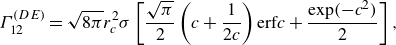 \begin{equation} \Gamma _{12}^{(DE)} = \sqrt {8\pi }r_c^2\sigma \left [\frac {\sqrt {\pi }}{2}\left (c + \frac {1}{2c}\right )\textrm {erf} c + \frac {\exp (-c^2)}{2}\right ], \end{equation}
where $c = |\tau _2 - \tau _1|\mathfrak{g}/(\sqrt {2}\sigma )$
and
$c = |\tau _2 - \tau _1|\mathfrak{g}/(\sqrt {2}\sigma )$
and $\sigma ^2 = r_c^2\varepsilon /(15\nu ) + 1.3(\tau _2 - \tau _1)^2\varepsilon ^{3/2}/\nu ^{1/2}$
. Crucially, they assumed that relative settling is captured by a shift in the mean vertical velocity while the variance remains unaffected. Consequently, their expression is consistent with Saffman & Turner (Reference Saffman and Turner1956) in the no-gravity limit. In the very large
$\sigma ^2 = r_c^2\varepsilon /(15\nu ) + 1.3(\tau _2 - \tau _1)^2\varepsilon ^{3/2}/\nu ^{1/2}$
. Crucially, they assumed that relative settling is captured by a shift in the mean vertical velocity while the variance remains unaffected. Consequently, their expression is consistent with Saffman & Turner (Reference Saffman and Turner1956) in the no-gravity limit. In the very large $St$
limit, where particles can be modelled as kinetic gases with normally distributed velocity components, Abrahamson (Reference Abrahamson1975) similarly accounted for gravity by shifting the vertical velocity p.d.f. of each species by the mean settling velocity so that
$St$
limit, where particles can be modelled as kinetic gases with normally distributed velocity components, Abrahamson (Reference Abrahamson1975) similarly accounted for gravity by shifting the vertical velocity p.d.f. of each species by the mean settling velocity so that
 \begin{align} \Gamma _{12} &= \pi r_c^2 v_c\nonumber \\ &= \frac {\pi r_c^2}{(2\pi v_1^{\prime 2})^{3/2}(2\pi v_2^{\prime 2})^{3/2}} \mathop{\int \!\!\int \!\!\int \!\!\int \!\!\int \!\!\int}\limits_{\textrm {all space}} \sqrt {(v_{1x}-v_{2x})^2 + (v_{1y}-v_{2y})^2 + (v_{1z}-v_{2z})^2}\nonumber \\ &\quad \times \exp {\left [\sum _{i = 1}^{2}-\frac {v_{ix}^2 + v_{iy}^2 + (v_{iz} - v_{Ti})^2}{2v_i^{\prime 2}} \right ]} \mathrm{d}v_{1x}\mathrm{d}v_{1y}\mathrm{d}v_{1z}\mathrm{d}v_{2x}\mathrm{d}v_{2y}\mathrm{d}v_{2z}, \end{align}
where $v_{x,y}$
and
$v_{x,y}$
and $v_{z}$
are the horizontal and the vertical particle velocity components, respectively. Abrahamson (Reference Abrahamson1975) evaluated the integral in (2.3) analytically and reported that
$v_{z}$
are the horizontal and the vertical particle velocity components, respectively. Abrahamson (Reference Abrahamson1975) evaluated the integral in (2.3) analytically and reported that
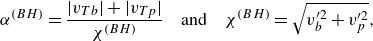
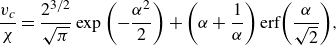 \begin{equation} \frac {v_c}{\chi } = \frac {2^{3/2}}{\sqrt {\pi }}\exp \left (-\frac {\alpha ^2}{2}\right ) + \left (\alpha + \frac {1}{\alpha }\right )\textrm {erf}{\left (\frac {\alpha }{\sqrt {2}}\right )}, \end{equation}
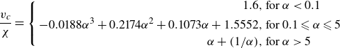
where
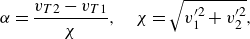 \begin{equation} \alpha = \frac {v_{T2}-v_{T1}}{\chi }, \quad \chi = \sqrt {v^{\prime 2}_1 + v^{\prime 2}_2}, \end{equation}
and $v^{\prime 2}_i$
is the mean-square single-component particle velocity. Unfortunately, the integration was not performed correctly so (2.4) does not reduce to the no-gravity case (
$v^{\prime 2}_i$
is the mean-square single-component particle velocity. Unfortunately, the integration was not performed correctly so (2.4) does not reduce to the no-gravity case ( $\Gamma _{12} = \sqrt {8\pi }r_c^2\sqrt {v^{\prime 2}_1 + v^{\prime 2}_2}$
) when
$\Gamma _{12} = \sqrt {8\pi }r_c^2\sqrt {v^{\prime 2}_1 + v^{\prime 2}_2}$
) when $\alpha \to 0$
because
$\alpha \to 0$
because $\lim _{\alpha \to 0} \textrm {erf}(\alpha )/\alpha$
does not converge to 0, as has already been pointed out by Kostoglou, Karapantsios & Evgenidis (Reference Kostoglou, Karapantsios and Evgenidis2020a
) and Kostoglou, Karapantsios & Oikonomidou (Reference Kostoglou, Karapantsios and Oikonomidou2020b
). Instead, we integrate (2.3) numerically and obtain the best-fit result
$\lim _{\alpha \to 0} \textrm {erf}(\alpha )/\alpha$
does not converge to 0, as has already been pointed out by Kostoglou, Karapantsios & Evgenidis (Reference Kostoglou, Karapantsios and Evgenidis2020a
) and Kostoglou, Karapantsios & Oikonomidou (Reference Kostoglou, Karapantsios and Oikonomidou2020b
). Instead, we integrate (2.3) numerically and obtain the best-fit result
 \begin{equation} \Gamma _{12} = \pi r_c^2 v_c ,\end{equation}
where
 \begin{equation} \frac {v_c}{\chi } = \left \{ \begin{aligned} 1.6, &\ \text{for $\alpha \lt 0.1$}\\ -0.0188\alpha ^3+0.2174\alpha ^2+0.1073\alpha +1.5552,&\ \text{for $0.1\leqslant \alpha \leqslant 5$}\\ \alpha + (1/\alpha ),&\ \text{for $\alpha \gt 5$} \end{aligned} \right . \end{equation}
and $\alpha$
and
$\alpha$
and $\chi$
are given by (2.5). Note that the coefficients for the
$\chi$
are given by (2.5). Note that the coefficients for the $\alpha \in [0.1,5]$
case of (2.7) are slightly different from the ones reported in Kostoglou et al. (Reference Kostoglou, Karapantsios and Evgenidis2020a
), presumably due to a typographical error (see Appendix A).
$\alpha \in [0.1,5]$
case of (2.7) are slightly different from the ones reported in Kostoglou et al. (Reference Kostoglou, Karapantsios and Evgenidis2020a
), presumably due to a typographical error (see Appendix A).
None of the above models account for the intricate interactions between the effects of turbulence and gravity, as pointed out by Woittiez, Jonker & Portela (Reference Woittiez, Jonker and Portela2009). This is particularly important for bidispersed particles whose motions are correlated. Essentially, the different settling speeds means that the two species do not have the same amount of time to interact with the fluid locally. This leads to a further decorrelation of their concentration fields (Woittiez et al. Reference Woittiez, Jonker and Portela2009; Dhariwal & Bragg Reference Dhariwal and Bragg2018), as well as increased collision velocity as particles attain high values of acceleration in the horizontal direction (Parishani et al. Reference Parishani, Ayala, Rosa, Wang and Grabowski2015; Dhariwal & Bragg Reference Dhariwal and Bragg2018), both of which affect the collision rate. Despite the limitations of the above models, we introduce them here as they form the basis for the existing bubble–particle collision models.
2.3. The effect of gravity on bubble–particle collisions
With gravity, bubbles rise and particles settle due to their relative density, meaning $v_{T1}$
and
$v_{T1}$
and $v_{T2}$
have opposite signs in (2.1) so relative settling is enhanced. Existing models for bubble–particle collisions are almost all direct extensions of those discussed in § 2.2. In the high
$v_{T2}$
have opposite signs in (2.1) so relative settling is enhanced. Existing models for bubble–particle collisions are almost all direct extensions of those discussed in § 2.2. In the high $St$
, ‘kinetic gas-like’ limit, Bloom & Heindel (Reference Bloom and Heindel2002) adapted (2.3)–(2.5) by simply replacing the settling velocities with the bubble (particle) rising (settling) velocity, meaning
$St$
, ‘kinetic gas-like’ limit, Bloom & Heindel (Reference Bloom and Heindel2002) adapted (2.3)–(2.5) by simply replacing the settling velocities with the bubble (particle) rising (settling) velocity, meaning
 \begin{equation} \alpha ^{(BH)} = \frac {|v_{Tb}|+|v_{Tp}|}{\chi ^{(BH)}} \quad \mathrm{and} \quad \chi ^{(BH)} = \sqrt {v^{\prime 2}_b + v^{\prime 2}_p}, \end{equation}
where the subscripts $b$
and
$b$
and $p$
denote ‘bubble’ and ‘particle’, respectively. Since Bloom & Heindel (Reference Bloom and Heindel2002) incorrectly used expressions for slip velocities in lieu of
$p$
denote ‘bubble’ and ‘particle’, respectively. Since Bloom & Heindel (Reference Bloom and Heindel2002) incorrectly used expressions for slip velocities in lieu of $v'_b$
and
$v'_b$
and $v'_p$
, as pointed out in Chan et al. (Reference Chan, Ng and Krug2023), in this work we employ the expression given by Abrahamson (Reference Abrahamson1975) in (2.8) for both
$v'_p$
, as pointed out in Chan et al. (Reference Chan, Ng and Krug2023), in this work we employ the expression given by Abrahamson (Reference Abrahamson1975) in (2.8) for both $v'_b$
and
$v'_b$
and $v'_p$
. For intermediate
$v'_p$
. For intermediate $St$
, Ngo-Cong, Nguyen & Tran-Cong (Reference Ngo-Cong, Nguyen and Tran-Cong2018) first modelled the zero-gravity bubble–particle velocity correlation following the approach of Yuu (Reference Yuu1984), such that the root mean square (r.m.s.) of the single-component bubble–particle relative velocity without gravity is
$St$
, Ngo-Cong, Nguyen & Tran-Cong (Reference Ngo-Cong, Nguyen and Tran-Cong2018) first modelled the zero-gravity bubble–particle velocity correlation following the approach of Yuu (Reference Yuu1984), such that the root mean square (r.m.s.) of the single-component bubble–particle relative velocity without gravity is $\sigma _{\Delta v}^{(NC)} = [(A_b + A_p - 2B)u^{\prime 2} + (A_br_b^2 + A_pr_p^2 + 2Br_pr_b)\varepsilon /(9\nu )]^{1/2}$
, where
$\sigma _{\Delta v}^{(NC)} = [(A_b + A_p - 2B)u^{\prime 2} + (A_br_b^2 + A_pr_p^2 + 2Br_pr_b)\varepsilon /(9\nu )]^{1/2}$
, where $u'$
is the single-component r.m.s. fluid velocity fluctuation, and
$u'$
is the single-component r.m.s. fluid velocity fluctuation, and $A_i$
and
$A_i$
and $B$
are coefficients that depend on particle properties and the fluid Lagrangian integral time scale. They then included gravity using (2.4) with
$B$
are coefficients that depend on particle properties and the fluid Lagrangian integral time scale. They then included gravity using (2.4) with
 \begin{equation} \alpha ^{(NC)} = \frac {|v_{Tb}|+|v_{Tp}|}{\chi ^{(NC)}} \quad \mathrm{and} \quad \chi ^{(NC)} = \sigma _{\Delta v}^{(NC)}. \end{equation}
We point out that (2.4) is derived from (2.3), which assumes uncorrelated particle velocities. The use of (2.4) at intermediate $St$
, where the correlation between particle velocities remains finite, is therefore inconsistent. In addition, both Bloom & Heindel (Reference Bloom and Heindel2002) and Ngo-Cong et al. (Reference Ngo-Cong, Nguyen and Tran-Cong2018) use the wrong integration result (2.4), such that these models also do not converge to the correct no-gravity limit. Expressions that have been corrected for this error are given by (2.6) and (2.7), along with (2.8) for Bloom & Heindel (Reference Bloom and Heindel2002) and (2.9) for Ngo-Cong et al. (Reference Ngo-Cong, Nguyen and Tran-Cong2018). For small
$St$
, where the correlation between particle velocities remains finite, is therefore inconsistent. In addition, both Bloom & Heindel (Reference Bloom and Heindel2002) and Ngo-Cong et al. (Reference Ngo-Cong, Nguyen and Tran-Cong2018) use the wrong integration result (2.4), such that these models also do not converge to the correct no-gravity limit. Expressions that have been corrected for this error are given by (2.6) and (2.7), along with (2.8) for Bloom & Heindel (Reference Bloom and Heindel2002) and (2.9) for Ngo-Cong et al. (Reference Ngo-Cong, Nguyen and Tran-Cong2018). For small $St$
, a consistent model for bubble–particle collisions in turbulence with gravity is missing to date. We extend the theory by Dodin & Elperin (Reference Dodin and Elperin2002) to the bubble–particle case (see Appendix B for details) and include a drag correction
$St$
, a consistent model for bubble–particle collisions in turbulence with gravity is missing to date. We extend the theory by Dodin & Elperin (Reference Dodin and Elperin2002) to the bubble–particle case (see Appendix B for details) and include a drag correction $f_i$
(
$f_i$
( $f_i = 1$
for Stokes drag) to obtain
$f_i = 1$
for Stokes drag) to obtain
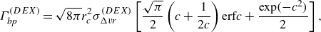 \begin{equation} \Gamma _{bp}^{(DEX)} = \sqrt {8\pi }r_c^2\sigma _{\Delta vr}^{(DEX)} \left [\frac {\sqrt {\pi }}{2}\left (c + \frac {1}{2c}\right )\textrm {erf} c + \frac {\exp (-c^2)}{2}\right ], \end{equation}
where
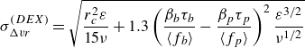 \begin{equation} \sigma _{\Delta vr}^{(DEX)} = \sqrt {\frac {r_c^2\varepsilon }{15\nu } + 1.3\left (\frac {\beta _b\tau _b}{\langle f_b\rangle } - \frac {\beta _p\tau _p}{\langle f_p\rangle }\right )^2\frac {\varepsilon ^{3/2}}{\nu ^{1/2}}} \end{equation}
is the r.m.s. of $\Delta v_r$
in zero gravity,
$\Delta v_r$
in zero gravity, $\beta_i = 2(\rho_f - \rho_i)/(\rho_f + 2\rho_i)$
,
$\beta_i = 2(\rho_f - \rho_i)/(\rho_f + 2\rho_i)$
,
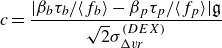 \begin{equation} c = \frac {|\beta _b\tau _b/\langle f_b\rangle - \beta _p\tau _p/\langle f_p\rangle |\mathfrak{g}}{\sqrt {2}\sigma _{\Delta vr}^{(DEX)}} \end{equation}
is the ratio of the relative settling velocity to the turbulence-induced radial collision velocity (up to a constant) and $\langle \cdot \rangle$
denotes averaging. This expression incorporates three collision mechanisms at small
$\langle \cdot \rangle$
denotes averaging. This expression incorporates three collision mechanisms at small $St$
: collision due to local fluid shear, local turnstile mechanism and relative settling. We note that Kostoglou et al. (Reference Kostoglou, Karapantsios and Evgenidis2020a
) proposed a model which considers a bubble in a swarm of tracers. However, since it does not decompose the collision process into the geometric collision rate and the collision efficiency, we do not further consider it in this study.
$St$
: collision due to local fluid shear, local turnstile mechanism and relative settling. We note that Kostoglou et al. (Reference Kostoglou, Karapantsios and Evgenidis2020a
) proposed a model which considers a bubble in a swarm of tracers. However, since it does not decompose the collision process into the geometric collision rate and the collision efficiency, we do not further consider it in this study.
While several models for bubble–particle collisions in turbulence that account for gravity are available, none of them have been directly tested. Even in zero gravity, the model predictions are hugely different from simulation results, which underscores the lack of understanding and the richness of the physics of bubble–particle collisions (Chan et al. Reference Chan, Ng and Krug2023). The only direct numerical study on bubble–particle geometric collisions with gravity in HIT that we are aware of does not vary $St$
,
$St$
, $Fr$
and
$Fr$
and $Re_\lambda$
independently (Wan et al. Reference Wan, Yi, Wang, Sun, Chen and Wang2020). The goal this work is therefore to systematically investigate the effect of
$Re_\lambda$
independently (Wan et al. Reference Wan, Yi, Wang, Sun, Chen and Wang2020). The goal this work is therefore to systematically investigate the effect of $St$
,
$St$
, $Fr$
and
$Fr$
and $Re_\lambda$
for bubble–particle collisions through simulations in order to reveal the underlying physical picture and assess the available models.
$Re_\lambda$
for bubble–particle collisions through simulations in order to reveal the underlying physical picture and assess the available models.
3. Methods
The simulations are performed using the same fluid and particle solvers as Chan et al. (Reference Chan, Ng and Krug2023). Hence, we only provide a brief summary here for completeness. For the background turbulence, we run direct numerical simulations of HIT using a finite-difference solver (second order in space, third order in time) to solve the incompressible Navier–Stokes and continuity equations
 \begin{align}& \frac {\mathrm{D}\boldsymbol{u}}{\mathrm{D}t} = -\frac {1}{\rho _f}\nabla P + \nu \nabla ^2\boldsymbol{u} + \boldsymbol{f_\Psi },\\[-10pt]\nonumber \end{align}
 \begin{align}&\qquad\qquad \nabla \boldsymbol{\cdot }\boldsymbol{u} =0, \end{align}
where $\mathrm{D}/\mathrm{D}t$
is the material derivative following a fluid element,
$\mathrm{D}/\mathrm{D}t$
is the material derivative following a fluid element, $\boldsymbol{u}$
is the fluid velocity,
$\boldsymbol{u}$
is the fluid velocity, $t$
is the time and
$t$
is the time and $P$
is the pressure. The fluid is forced randomly at the largest scales
$P$
is the pressure. The fluid is forced randomly at the largest scales $\boldsymbol{f_\Psi }$
using the scheme by Eswaran & Pope (Reference Eswaran and Pope1988) to generate turbulence with
$\boldsymbol{f_\Psi }$
using the scheme by Eswaran & Pope (Reference Eswaran and Pope1988) to generate turbulence with $Re_\lambda = 69$
and
$Re_\lambda = 69$
and $167$
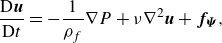
. Other turbulence statistics are displayed in table 1. We also show in figure 1 that the power spectrum agrees excellently with that of Jiménez et al. (Reference Jiménez, Wray, Saffman and Rogallo1993).
$167$
. Other turbulence statistics are displayed in table 1. We also show in figure 1 that the power spectrum agrees excellently with that of Jiménez et al. (Reference Jiménez, Wray, Saffman and Rogallo1993).
Table 1. Statistics of HIT: the grid size ( $\textbf{N}$
), pseudo-dissipation (
$\textbf{N}$
), pseudo-dissipation ( $\overline {\varepsilon }$
), Kolmogorov length scale (
$\overline {\varepsilon }$
), Kolmogorov length scale ( $\eta$
), maximum wavenumber (
$\eta$
), maximum wavenumber ( $k_{max}$
), Kolmogorov velocity (
$k_{max}$
), Kolmogorov velocity ( $u_\eta$
) scale, r.m.s. velocity fluctuations (
$u_\eta$
) scale, r.m.s. velocity fluctuations ( $u'$
), large-scale isotropy (
$u'$
), large-scale isotropy ( $u_x'/u_y'$
) and the large eddy turnover time (
$u_x'/u_y'$
) and the large eddy turnover time ( $T_L$
) relative to the Kolmogorov time scale (
$T_L$
) relative to the Kolmogorov time scale ( $\tau _\eta$
). Here,
$\tau _\eta$
). Here, $N_{b,p}$
are the numbers of bubbles and particles, respectively. The simulations including the history force have the same parameters as the
$N_{b,p}$
are the numbers of bubbles and particles, respectively. The simulations including the history force have the same parameters as the $Re_\lambda = 167$
case except for a lower number of bubbles and particles
$Re_\lambda = 167$
case except for a lower number of bubbles and particles $N_{b,p} = 50\,000$
.
$N_{b,p} = 50\,000$
.

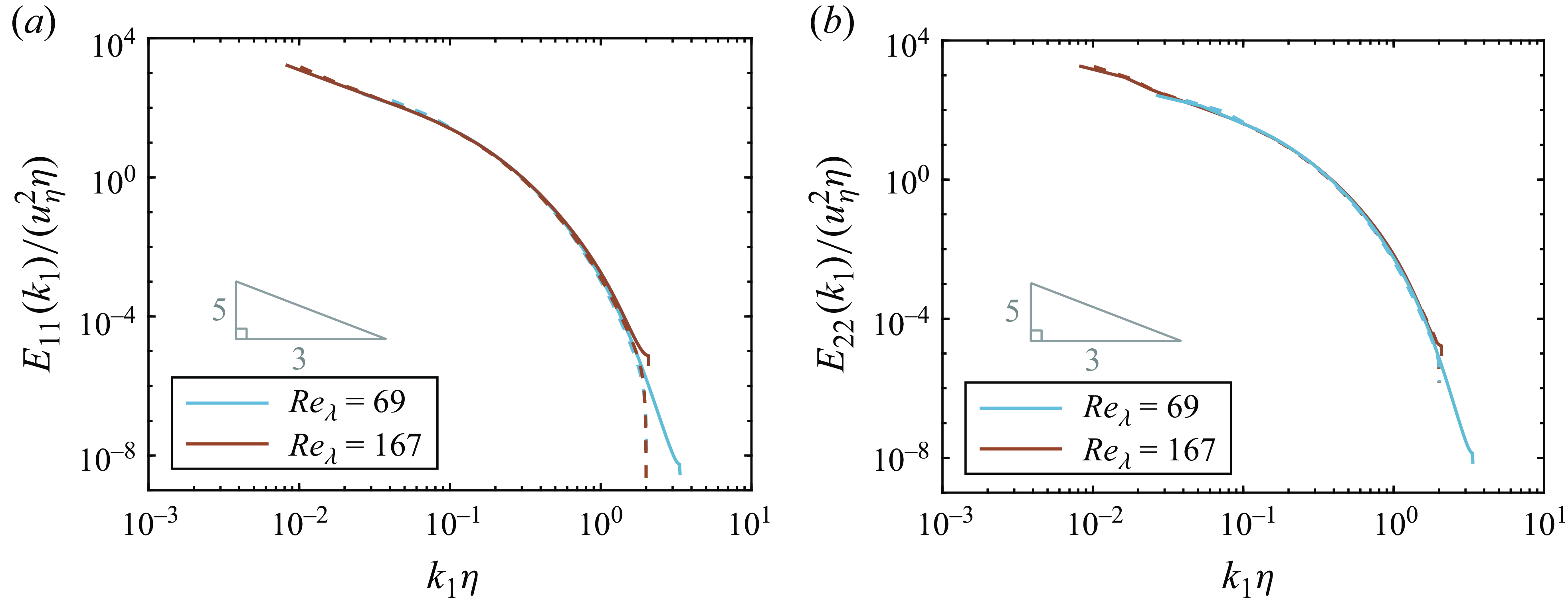
Figure 1. The (a) longitudinal and (b) transverse energy spectra. The dashed lines show data from Jiménez et al. (Reference Jiménez, Wray, Saffman and Rogallo1993) for $Re_\lambda = 62.7$
(in blue) and
$Re_\lambda = 62.7$
(in blue) and $170.2$
(in brown).
$170.2$
(in brown).
For the bubbles and particles, we approximate them using the point-particle approach (for a historical overview of this approach, see Michaelides Reference Michaelides2003) which implies that both species are modelled as rigid spheres. This is reasonable even for the bubbles since the Weber number based on their rise velocity at $(St_b, 1/Fr, Re_\lambda ) = (11, 4.4, 64)$
is O(0.1) (Jiang & Krug Reference Jiang and Krug2025). As described later in this section, this work focuses on bubbles with lower values of
$(St_b, 1/Fr, Re_\lambda ) = (11, 4.4, 64)$
is O(0.1) (Jiang & Krug Reference Jiang and Krug2025). As described later in this section, this work focuses on bubbles with lower values of $St_b$
, such that the bubble radii and rise velocities are smaller at comparable values of
$St_b$
, such that the bubble radii and rise velocities are smaller at comparable values of $1/Fr$
, thus bubble deformation is even less significant. Under the point-particle approach (Gatignol Reference Gatignol1983; Maxey & Riley Reference Maxey and Riley1983; Auton et al. Reference Auton, Hunt and Prud’Homme1988), the net force on the particle is the sum of the drag force, the pressure gradient force, the added mass force, buoyancy, lift (Auton Reference Auton1987), the history force and Faxén terms. We initially neglect the history force and Faxén terms to allow fair comparison with the models introduced in § 2.3. A finite-difference solver is used to solve
$1/Fr$
, thus bubble deformation is even less significant. Under the point-particle approach (Gatignol Reference Gatignol1983; Maxey & Riley Reference Maxey and Riley1983; Auton et al. Reference Auton, Hunt and Prud’Homme1988), the net force on the particle is the sum of the drag force, the pressure gradient force, the added mass force, buoyancy, lift (Auton Reference Auton1987), the history force and Faxén terms. We initially neglect the history force and Faxén terms to allow fair comparison with the models introduced in § 2.3. A finite-difference solver is used to solve
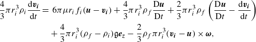 \begin{align} \frac {4}{3}\pi r_i^3\rho _i\frac {\mathrm{d}\boldsymbol{v_i}}{\mathrm{d}t} & =\, 6\pi \mu r_if_i(\boldsymbol{u}-\boldsymbol{v_i}) + \frac {4}{3}\pi r_i^3\rho _f\frac {\mathrm{D}\boldsymbol{u}}{\mathrm{D}t} + \frac {2}{3}\pi r_i^3\rho _f\left (\frac {\mathrm{D}\boldsymbol{u}}{\mathrm{D}t} - \frac {\mathrm{d}\boldsymbol{v_i}}{\mathrm{d}t}\right )\nonumber \\ &\quad + \frac {4}{3}\pi r_i^3(\rho _f - \rho _i)\mathfrak{g}\boldsymbol{e_z} - \frac {2}{3}\rho _f\pi r_i^3(\boldsymbol{v_i} - \boldsymbol{u})\times \boldsymbol{\omega }, \end{align}
where $\boldsymbol{v_i}$
is the particle velocity,
$\boldsymbol{v_i}$
is the particle velocity, $\mu =\nu \rho _f$
is the absolute viscosity,
$\mu =\nu \rho _f$
is the absolute viscosity, $\boldsymbol{e_z}$
is the unit vector pointing vertically upwards,
$\boldsymbol{e_z}$
is the unit vector pointing vertically upwards, $\boldsymbol{\omega }$
is the vorticity vector and
$\boldsymbol{\omega }$
is the vorticity vector and $f_i = 1 + 0.169Re_i^{2/3}$
is the correction factor that accounts for nonlinear drag due to finite bubble or particle Reynolds number
$f_i = 1 + 0.169Re_i^{2/3}$
is the correction factor that accounts for nonlinear drag due to finite bubble or particle Reynolds number $Re_i = 2r_i|\boldsymbol{u - v_i}|/\nu$
and implies a no-slip boundary condition (Nguyen & Schulze Reference Nguyen and Schulze2004). Here,
$Re_i = 2r_i|\boldsymbol{u - v_i}|/\nu$
and implies a no-slip boundary condition (Nguyen & Schulze Reference Nguyen and Schulze2004). Here, $r_i$
is determined from (1.4), while
$r_i$
is determined from (1.4), while $\boldsymbol{u}$
,
$\boldsymbol{u}$
, $\mathrm{D}\boldsymbol{u}/\mathrm{D}t$
and
$\mathrm{D}\boldsymbol{u}/\mathrm{D}t$
and $\boldsymbol{\omega }$
at the particle positions are evaluated using tri-cubic Hermite spline interpolation with a stencil of four points per direction (van Hinsberg et al. Reference van Hinsberg, ten Thije Boonkkamp, Toschi and Clercx2013). We employ a lift coefficient
$\boldsymbol{\omega }$
at the particle positions are evaluated using tri-cubic Hermite spline interpolation with a stencil of four points per direction (van Hinsberg et al. Reference van Hinsberg, ten Thije Boonkkamp, Toschi and Clercx2013). We employ a lift coefficient $C_L$
of 1/2, which strictly speaking is only valid for clean bubbles with very large
$C_L$
of 1/2, which strictly speaking is only valid for clean bubbles with very large $Re_b$
in simple shear flows (Auton Reference Auton1987; Legendre & Magnaudet Reference Legendre and Magnaudet1998), and acknowledge that the actual value depends on the type of flow and
$Re_b$
in simple shear flows (Auton Reference Auton1987; Legendre & Magnaudet Reference Legendre and Magnaudet1998), and acknowledge that the actual value depends on the type of flow and $Re_b$
(Legendre & Magnaudet Reference Legendre and Magnaudet1998; Magnaudet & Legendre Reference Magnaudet and Legendre1998). Nonetheless, we use
$Re_b$
(Legendre & Magnaudet Reference Legendre and Magnaudet1998; Magnaudet & Legendre Reference Magnaudet and Legendre1998). Nonetheless, we use $C_L = 1/2$
following Mazzitelli & Lohse (Reference Mazzitelli and Lohse2004), who simulated similar bubbles in HIT. Although we initially neglect the history force, we recognise that it may play a noticeable role in reality for our tested bubble and particle density ratios (Olivieri et al. Reference Olivieri, Picano, Sardina, Iudicone and Brandt2014; Daitche Reference Daitche2015). We therefore run additional cases in § 4.5 with the history force
$C_L = 1/2$
following Mazzitelli & Lohse (Reference Mazzitelli and Lohse2004), who simulated similar bubbles in HIT. Although we initially neglect the history force, we recognise that it may play a noticeable role in reality for our tested bubble and particle density ratios (Olivieri et al. Reference Olivieri, Picano, Sardina, Iudicone and Brandt2014; Daitche Reference Daitche2015). We therefore run additional cases in § 4.5 with the history force
 \begin{equation} \boldsymbol{F_{hist}} = 6r_i^2\rho _f\sqrt {\pi \nu }\int _{0}^{t} \frac {\frac {\mathrm{d} (\boldsymbol{u}(\tau ) - \boldsymbol{v_i}(\tau ))}{\mathrm{d}\tau }}{\sqrt {t-\tau }}\mathrm{d}\tau \end{equation}
added to the right-hand side of (3.2). The value of $\boldsymbol{F_{hist}}$
is computed using the semi-implicit scheme by van Hinsberg, ten Thije Boonkkamp & Clercx (Reference van Hinsberg, ten Thije Boonkkamp and Clercx2011), where a window length of 5 time steps is chosen and the tail of the integrand is modelled with 10 exponential functions. Hence, the results are comparable to a simple window method (Dorgan & Loth Reference Dorgan and Loth2007) where the integration is truncated to the last 500 time steps (van Hinsberg et al. Reference van Hinsberg, ten Thije Boonkkamp and Clercx2011). This corresponds to approximately
$\boldsymbol{F_{hist}}$
is computed using the semi-implicit scheme by van Hinsberg, ten Thije Boonkkamp & Clercx (Reference van Hinsberg, ten Thije Boonkkamp and Clercx2011), where a window length of 5 time steps is chosen and the tail of the integrand is modelled with 10 exponential functions. Hence, the results are comparable to a simple window method (Dorgan & Loth Reference Dorgan and Loth2007) where the integration is truncated to the last 500 time steps (van Hinsberg et al. Reference van Hinsberg, ten Thije Boonkkamp and Clercx2011). This corresponds to approximately $9\tau _\eta$
, which Calzavarini et al. (Reference Calzavarini, Volk, Lévêque, Pinton and Toschi2012) found is long enough for the integrand to decay to negligible values in HIT for their parameters.
$9\tau _\eta$
, which Calzavarini et al. (Reference Calzavarini, Volk, Lévêque, Pinton and Toschi2012) found is long enough for the integrand to decay to negligible values in HIT for their parameters.
In all our simulations, the collisions are treated using the ‘ghost collision’ scheme as it is consistent with the models described in § 2 (Wang, Wexler & Zhou Reference Wang, Wexler and Zhou1998). This means particles can overlap and a collision is registered every time an approaching pair of particles reaches the collision distance $r_c$
, which is set to
$r_c$
, which is set to $r_b + r_p$
for all species. We eliminate wall effects by implementing periodic boundary conditions in all directions and verified that the domain size
$r_b + r_p$
for all species. We eliminate wall effects by implementing periodic boundary conditions in all directions and verified that the domain size $L_{box} = 1$
is sufficiently large to minimise periodicity effects (see Appendix C). The time step
$L_{box} = 1$
is sufficiently large to minimise periodicity effects (see Appendix C). The time step $\Delta t \leqslant \tau _\eta /55$
is sufficiently small such that the Courant–Friedrichs–Lewy (CFL) number
$\Delta t \leqslant \tau _\eta /55$
is sufficiently small such that the Courant–Friedrichs–Lewy (CFL) number $ \leqslant 1$
(apart from a few time steps for the cases in §§ 4.4 and 4.5) and the point-particle statistics are no longer sensitive to
$ \leqslant 1$
(apart from a few time steps for the cases in §§ 4.4 and 4.5) and the point-particle statistics are no longer sensitive to $\Delta t$
(Ruth et al. Reference Ruth, Vernet, Perrard and Deike2021). We refer the reader to Chan et al. (Reference Chan, Ng and Krug2023) for details of the solvers and the collision detection algorithm.
$\Delta t$
(Ruth et al. Reference Ruth, Vernet, Perrard and Deike2021). We refer the reader to Chan et al. (Reference Chan, Ng and Krug2023) for details of the solvers and the collision detection algorithm.
We investigate bubbles ( $\rho _b/\rho _f = 1/1000$
) and particles (
$\rho _b/\rho _f = 1/1000$
) and particles ( $\rho _p/\rho _f = 5$
) with
$\rho _p/\rho _f = 5$
) with $St$
of 0.1, 0.5, 1, 2 and 3, and
$St$
of 0.1, 0.5, 1, 2 and 3, and $1/Fr$
ranging from 0.01 to 10. For the bubbles, these values of
$1/Fr$
ranging from 0.01 to 10. For the bubbles, these values of $St$
correspond to
$St$
correspond to $r_b/\eta = 0.9$
, 2.2, 3.0, 4.2 and 5.2, respectively; and it should be noted that finite-size effects, that are not represented in our computations, may become relevant in particular at the larger values of
$r_b/\eta = 0.9$
, 2.2, 3.0, 4.2 and 5.2, respectively; and it should be noted that finite-size effects, that are not represented in our computations, may become relevant in particular at the larger values of $St$
. Nonetheless, we believe that our approach still allows us to examine the general trend with increasing
$St$
. Nonetheless, we believe that our approach still allows us to examine the general trend with increasing $St$
and to assess the collision models introduced in § 2.3, which also do not include these effects. We consider only
$St$
and to assess the collision models introduced in § 2.3, which also do not include these effects. We consider only $St_b = St_p$
to limit the parameter space. While this is not the most general case, it is physically relevant, especially in the context of flotation of fine particles, where small bubbles are preferred (Ahmed & Jameson Reference Ahmed and Jameson1985; Miettinen, Ralston & Fornasiero Reference Miettinen, Ralston and Fornasiero2010; Farrokhpay, Filippov & Fornasiero Reference Farrokhpay, Filippov and Fornasiero2021). The simulation is conducted as follows: bubbles and particles,
$St_b = St_p$
to limit the parameter space. While this is not the most general case, it is physically relevant, especially in the context of flotation of fine particles, where small bubbles are preferred (Ahmed & Jameson Reference Ahmed and Jameson1985; Miettinen, Ralston & Fornasiero Reference Miettinen, Ralston and Fornasiero2010; Farrokhpay, Filippov & Fornasiero Reference Farrokhpay, Filippov and Fornasiero2021). The simulation is conducted as follows: bubbles and particles, $10\,000{-}140\,000$
per species, are injected in the simulation domain at random positions after the flow has reached statistical stationarity. We then monitor the particle position p.d.f., particle velocity p.d.f. and the ensemble-average rise/settling velocities to identify transients. Once the transient states have passed, we collect statistics over at least
$10\,000{-}140\,000$
per species, are injected in the simulation domain at random positions after the flow has reached statistical stationarity. We then monitor the particle position p.d.f., particle velocity p.d.f. and the ensemble-average rise/settling velocities to identify transients. Once the transient states have passed, we collect statistics over at least $12.4$
large eddy turnover times (
$12.4$
large eddy turnover times ( $T_L$
) at a minimum sampling frequency of once per
$T_L$
) at a minimum sampling frequency of once per $0.06 T_L$
.
$0.06 T_L$
.
4. Results
4.1. Collision kernel
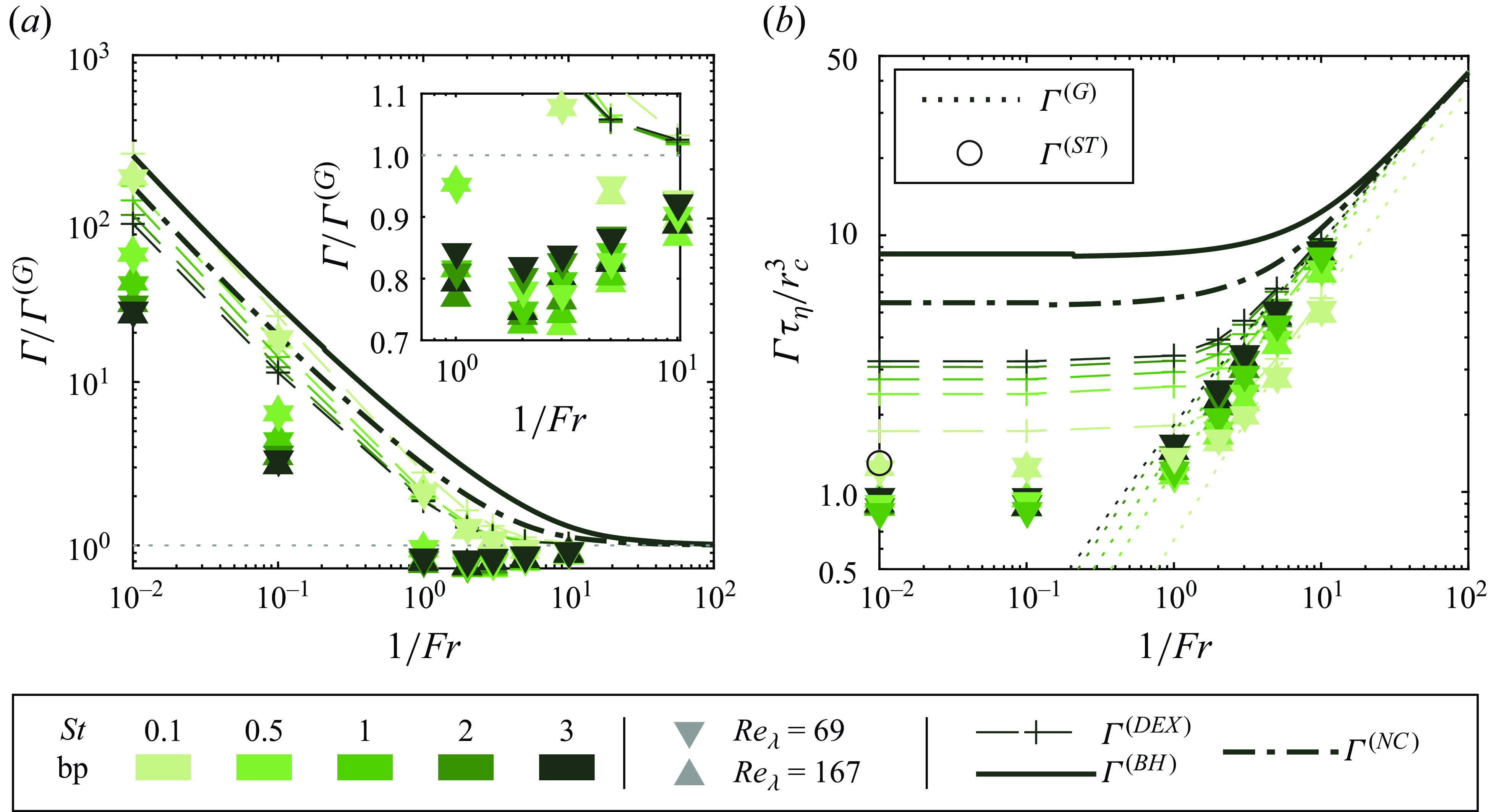
Figure 2. (a) The bubble–particle collision kernel normalised by the result for the relative settling case in still fluid. The inset shows a close-up view of the region where $1/Fr \geqslant 1$
. (b) The bubble–particle collision kernel normalised by
$1/Fr \geqslant 1$
. (b) The bubble–particle collision kernel normalised by $r_c^3/\tau _\eta$
. Here,
$r_c^3/\tau _\eta$
. Here, $\Gamma ^{(BH)}$
and
$\Gamma ^{(BH)}$
and $\Gamma ^{(NC)}$
(only shown for
$\Gamma ^{(NC)}$
(only shown for $St = 3$
) are computed using the corrected best-fit (2.7). The model predictions are for
$St = 3$
) are computed using the corrected best-fit (2.7). The model predictions are for $Re_\lambda = 167$
.
$Re_\lambda = 167$
.
Figure 2(a) presents results for the bubble–particle collision kernel normalised by the relative settling case in still fluid $\Gamma ^{(G)}$
, wherein the terminal velocities
$\Gamma ^{(G)}$
, wherein the terminal velocities $v_{Ti}$
are obtained by balancing buoyancy with the nonlinear drag term as shown by (3.2). At small
$v_{Ti}$
are obtained by balancing buoyancy with the nonlinear drag term as shown by (3.2). At small $1/Fr$
(weak gravity),
$1/Fr$
(weak gravity), $\Gamma /\Gamma ^{(G)}$
is large since bubbles and particles rise and settle very slowly such that
$\Gamma /\Gamma ^{(G)}$
is large since bubbles and particles rise and settle very slowly such that $\Gamma ^{(G)}$
is small and the collision rate is dominated by turbulence mechanisms. In this regime,
$\Gamma ^{(G)}$
is small and the collision rate is dominated by turbulence mechanisms. In this regime, $\Gamma /\Gamma ^{(G)}$
reduces with increasing
$\Gamma /\Gamma ^{(G)}$
reduces with increasing $St$
primarily because the rise and settling speeds
$St$
primarily because the rise and settling speeds $|v_{Ti}|$
are proportional to
$|v_{Ti}|$
are proportional to $St$
. As
$St$
. As $1/Fr$
increases, bubbles and particles rise and settle faster, enhancing the role of relative settling in the overall collision rate as reflected by a decreasing
$1/Fr$
increases, bubbles and particles rise and settle faster, enhancing the role of relative settling in the overall collision rate as reflected by a decreasing $\Gamma /\Gamma ^{(G)}$
such that, at large
$\Gamma /\Gamma ^{(G)}$
such that, at large $1/Fr$
,
$1/Fr$
, $\Gamma \approx \Gamma ^{(G)}$
. At close inspection, however,
$\Gamma \approx \Gamma ^{(G)}$
. At close inspection, however, $\Gamma \lt \Gamma ^{(G)}$
when
$\Gamma \lt \Gamma ^{(G)}$
when $1/Fr \gtrsim 5$
for
$1/Fr \gtrsim 5$
for $St = 0.1$
and
$St = 0.1$
and $1/Fr \gtrsim 1$
for
$1/Fr \gtrsim 1$
for $St \geqslant 0.5$
, as shown in the inset. This implies that, counter-intuitively, the presence of turbulence decreases the collision rate below the relative settling case in this regime. This is attributed to the non-uniform bubble–particle spatial distribution and their resulting segregation, and to the reduced bubble slip velocity due to nonlinear drag, as will be discussed further in §§ 4.2 and 4.3. As the segregation does not monotonically depend on
$St \geqslant 0.5$
, as shown in the inset. This implies that, counter-intuitively, the presence of turbulence decreases the collision rate below the relative settling case in this regime. This is attributed to the non-uniform bubble–particle spatial distribution and their resulting segregation, and to the reduced bubble slip velocity due to nonlinear drag, as will be discussed further in §§ 4.2 and 4.3. As the segregation does not monotonically depend on $St$
, there is no simple dependence between
$St$
, there is no simple dependence between $\Gamma /\Gamma ^{(G)}$
and
$\Gamma /\Gamma ^{(G)}$
and $St$
in this regime. Throughout the tested range of
$St$
in this regime. Throughout the tested range of $1/Fr$
and
$1/Fr$
and $Re_\lambda$
,
$Re_\lambda$
, $\Gamma /\Gamma ^{(G)}$
is not sensitive to
$\Gamma /\Gamma ^{(G)}$
is not sensitive to $Re_\lambda$
.
$Re_\lambda$
.
All the models considered successfully capture the general decreasing trend of $\Gamma /\Gamma ^{(G)}$
and the relative settling limit
$\Gamma /\Gamma ^{(G)}$
and the relative settling limit $\Gamma \to \Gamma ^{(G)}$
at
$\Gamma \to \Gamma ^{(G)}$
at $1/Fr \to \infty$
. However, the model predictions remain above
$1/Fr \to \infty$
. However, the model predictions remain above $\Gamma ^{(G)}$
over the entire range of
$\Gamma ^{(G)}$
over the entire range of $1/Fr$
even though the nonlinear drag expression has already been included. This is because they assume a uniform bubble–particle distribution and employ the bubble rise velocity in still fluid. As mentioned at the end of the last paragraph, this is not true from the simulations and will be elaborated on in §§ 4.2 and 4.3.
$1/Fr$
even though the nonlinear drag expression has already been included. This is because they assume a uniform bubble–particle distribution and employ the bubble rise velocity in still fluid. As mentioned at the end of the last paragraph, this is not true from the simulations and will be elaborated on in §§ 4.2 and 4.3.
We now normalise the collision kernel by $\tau _\eta /r_c^3$
, i.e. the scaling of
$\tau _\eta /r_c^3$
, i.e. the scaling of $\Gamma ^{(ST)}$
, in figure 2(b) to better examine the turbulence-to-relative settling transition. When
$\Gamma ^{(ST)}$
, in figure 2(b) to better examine the turbulence-to-relative settling transition. When $1/Fr \lesssim 0.1$
, bubble and particle dynamics is turbulence dominated and the results are consistent with Chan et al. (Reference Chan, Ng and Krug2023): the collision kernel coincides with
$1/Fr \lesssim 0.1$
, bubble and particle dynamics is turbulence dominated and the results are consistent with Chan et al. (Reference Chan, Ng and Krug2023): the collision kernel coincides with $\Gamma ^{(ST)}$
at small
$\Gamma ^{(ST)}$
at small $St$
and
$St$
and $\Gamma ^{(NC)}$
and
$\Gamma ^{(NC)}$
and $\Gamma ^{(BH)}$
overpredict the collision kernel. We stress, however, that the agreement with
$\Gamma ^{(BH)}$
overpredict the collision kernel. We stress, however, that the agreement with $\Gamma ^{(ST)}$
is merely a coincidence since the model does not account for bubble–particle segregation, as discussed in Chan et al. (Reference Chan, Ng and Krug2023). When
$\Gamma ^{(ST)}$
is merely a coincidence since the model does not account for bubble–particle segregation, as discussed in Chan et al. (Reference Chan, Ng and Krug2023). When $1/Fr$
increases, the effect of gravity on the collision kernel becomes noticeable and causes it to increase towards
$1/Fr$
increases, the effect of gravity on the collision kernel becomes noticeable and causes it to increase towards $\Gamma ^{(G)}$
. In the tested parameter range,
$\Gamma ^{(G)}$
. In the tested parameter range, $\Gamma$
is only weakly sensitive to
$\Gamma$
is only weakly sensitive to $Re_\lambda$
. Among the models,
$Re_\lambda$
. Among the models, $\Gamma ^{(DEX)}$
best matches the data for the parameters investigated. This is expected since it has been developed for the small
$\Gamma ^{(DEX)}$
best matches the data for the parameters investigated. This is expected since it has been developed for the small $St$
limit and has been extended to the bubble–particle case to also incorporate the local turnstile mechanism. On the other hand, Bloom & Heindel (Reference Bloom and Heindel2002) is applicable for the large
$St$
limit and has been extended to the bubble–particle case to also incorporate the local turnstile mechanism. On the other hand, Bloom & Heindel (Reference Bloom and Heindel2002) is applicable for the large $St$
kinetic gas limit which is inaccessible with the point-particle approach. Nonetheless, even for the
$St$
kinetic gas limit which is inaccessible with the point-particle approach. Nonetheless, even for the $St = 0.1$
case
$St = 0.1$
case $\Gamma ^{(DEX)}$
does not quantitatively agree with the data, presumably due to preferential sampling, as will be examined in the following section.
$\Gamma ^{(DEX)}$
does not quantitatively agree with the data, presumably due to preferential sampling, as will be examined in the following section.
4.2. Bubble–particle distribution
In zero gravity, bubbles and particles with small or moderate $St$
preferentially sample different flow regions in HIT due to different relative densities and form respective clusters at regions of high and low rotation rates, meaning they segregate (Calzavarini et al. Reference Calzavarini, Cencini, Lohse and Toschi2008). This effect has been shown to be most pronounced at
$St$
preferentially sample different flow regions in HIT due to different relative densities and form respective clusters at regions of high and low rotation rates, meaning they segregate (Calzavarini et al. Reference Calzavarini, Cencini, Lohse and Toschi2008). This effect has been shown to be most pronounced at $St = 1$
(Chan et al. Reference Chan, Ng and Krug2023). To examine the effect of gravity on the spatial distribution of bubbles and particles, figure 3 displays the instantaneous snapshots of the simulation with
$St = 1$
(Chan et al. Reference Chan, Ng and Krug2023). To examine the effect of gravity on the spatial distribution of bubbles and particles, figure 3 displays the instantaneous snapshots of the simulation with $St = 1$
over a range of
$St = 1$
over a range of $1/Fr$
. As
$1/Fr$
. As $1/Fr$
becomes larger, the overlap between bubble and particle positions increases. However, we do not observe a clear elongation of the bubble and particle clusters in the vertical direction, in contrast to other studies of heavy particles in turbulence (Bec et al. Reference Bec, Homann and Ray2014; Ireland et al. Reference Ireland, Bragg and Collins2016b
; Falkinhoff et al. Reference Falkinhoff, Obligado, Bourgoin and Mininni2020). This is because these studies employed a higher
$1/Fr$
becomes larger, the overlap between bubble and particle positions increases. However, we do not observe a clear elongation of the bubble and particle clusters in the vertical direction, in contrast to other studies of heavy particles in turbulence (Bec et al. Reference Bec, Homann and Ray2014; Ireland et al. Reference Ireland, Bragg and Collins2016b
; Falkinhoff et al. Reference Falkinhoff, Obligado, Bourgoin and Mininni2020). This is because these studies employed a higher $\rho _p$
, which enhances the overall effect of gravity. To more quantitatively investigate the locations sampled by bubbles and particles, we consider the theory by Bec et al. (Reference Bec, Homann and Ray2014), which predicts that a negative horizontal divergence of
$\rho _p$
, which enhances the overall effect of gravity. To more quantitatively investigate the locations sampled by bubbles and particles, we consider the theory by Bec et al. (Reference Bec, Homann and Ray2014), which predicts that a negative horizontal divergence of $\boldsymbol{v_p}$
occurs on average in downward flows when particles are settling in turbulence, i.e. ‘preferentially sweeping’ (Wang & Maxey Reference Wang and Maxey1993). Extending this reasoning to buoyant bubbles would mean that bubbles also cluster in downflow regions. Furthermore, the lift force pulls rising bubbles toward the downward branches of vortices (Mazzitelli, Lohse & Toschi Reference Mazzitelli, Lohse and Toschi2003). Collectively, this implies bubbles and particles sample downward flows in turbulence due to gravity. We test this hypothesis by plotting the mean vertical fluid velocity at bubble and particle positions in figure 4(a) and show that this is indeed the case for
$\boldsymbol{v_p}$
occurs on average in downward flows when particles are settling in turbulence, i.e. ‘preferentially sweeping’ (Wang & Maxey Reference Wang and Maxey1993). Extending this reasoning to buoyant bubbles would mean that bubbles also cluster in downflow regions. Furthermore, the lift force pulls rising bubbles toward the downward branches of vortices (Mazzitelli, Lohse & Toschi Reference Mazzitelli, Lohse and Toschi2003). Collectively, this implies bubbles and particles sample downward flows in turbulence due to gravity. We test this hypothesis by plotting the mean vertical fluid velocity at bubble and particle positions in figure 4(a) and show that this is indeed the case for $St/Fr \gtrsim 10^{-1}$
, with bubbles sampling regions with stronger downflow than particles. Additionally, the figure shows that
$St/Fr \gtrsim 10^{-1}$
, with bubbles sampling regions with stronger downflow than particles. Additionally, the figure shows that $\langle u_z \rangle _i$
collapses especially for
$\langle u_z \rangle _i$
collapses especially for $St \geqslant 0.5$
when plotted against
$St \geqslant 0.5$
when plotted against $St/Fr$
, which echoes the finding by Good et al. (Reference Good, Ireland, Bewley, Bodenschatz, Collins and Warhaft2014) that
$St/Fr$
, which echoes the finding by Good et al. (Reference Good, Ireland, Bewley, Bodenschatz, Collins and Warhaft2014) that $St/Fr$
is a key indicator of different particle settling regimes. To single out the colliding bubbles and particles, we condition the fluid velocity on pairs that are close to the collision distance in figure 4(b). We observe that the colliding pairs also preferentially sample downflow regions, and
$St/Fr$
is a key indicator of different particle settling regimes. To single out the colliding bubbles and particles, we condition the fluid velocity on pairs that are close to the collision distance in figure 4(b). We observe that the colliding pairs also preferentially sample downflow regions, and $\langle u_z \rangle _i|_{col}$
essentially takes the unconditioned bubble values
$\langle u_z \rangle _i|_{col}$
essentially takes the unconditioned bubble values $\langle u_z \rangle _b$
. This suggests that the bubble–particle collisions occur mainly at the unconditioned bubble positions such that the collision rate depends on the location of the particle clusters relative to the bubbles. To further examine this, we plot the norm of the rotation rate
$\langle u_z \rangle _b$
. This suggests that the bubble–particle collisions occur mainly at the unconditioned bubble positions such that the collision rate depends on the location of the particle clusters relative to the bubbles. To further examine this, we plot the norm of the rotation rate $\langle R^2 \rangle$
at bubble and particle positions in figure 4(c). When gravity is weak, bubbles and particles preferentially sample regions with high and low
$\langle R^2 \rangle$
at bubble and particle positions in figure 4(c). When gravity is weak, bubbles and particles preferentially sample regions with high and low $\langle R^2 \rangle$
values, respectively. As gravity becomes stronger, the values of both particle and (to a lesser extent) bubble
$\langle R^2 \rangle$
values, respectively. As gravity becomes stronger, the values of both particle and (to a lesser extent) bubble $\langle R^2 \rangle$
begin to return to the tracer limit of 0.5, which indicates a change in the clustering location and/or bubbles and particles cluster less.
$\langle R^2 \rangle$
begin to return to the tracer limit of 0.5, which indicates a change in the clustering location and/or bubbles and particles cluster less.
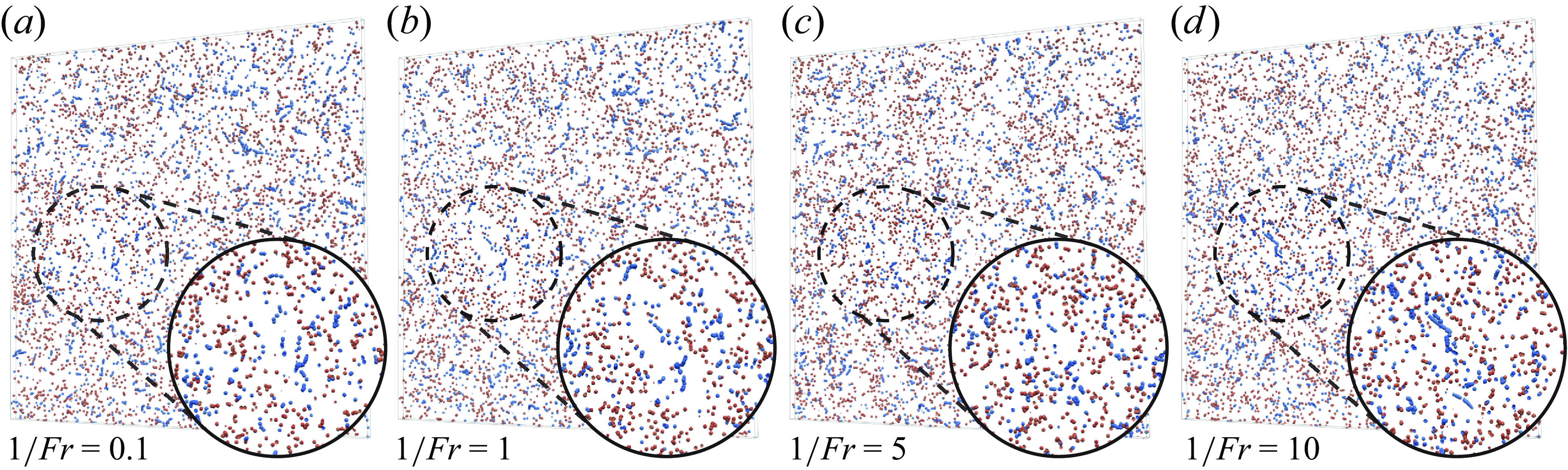
Figure 3. Instantaneous snapshots of bubbles (blue) and particles (red) in a slice with width $\times$
height
$\times$
height $\times$
depth =
$\times$
depth = $L_{box} \times L_{box} \times 20\eta$
with
$L_{box} \times L_{box} \times 20\eta$
with $Re_\lambda = 167$
,
$Re_\lambda = 167$
, $St = 1$
and (a)
$St = 1$
and (a) $1/Fr = 0.1$
, (b)
$1/Fr = 0.1$
, (b) $1/Fr = 1$
, (c)
$1/Fr = 1$
, (c) $1/Fr = 5$
and (d)
$1/Fr = 5$
and (d) $1/Fr = 10$
. Gravity is directed vertically downwards. The sizes of the bubbles and particles are not to scale.
$1/Fr = 10$
. Gravity is directed vertically downwards. The sizes of the bubbles and particles are not to scale.
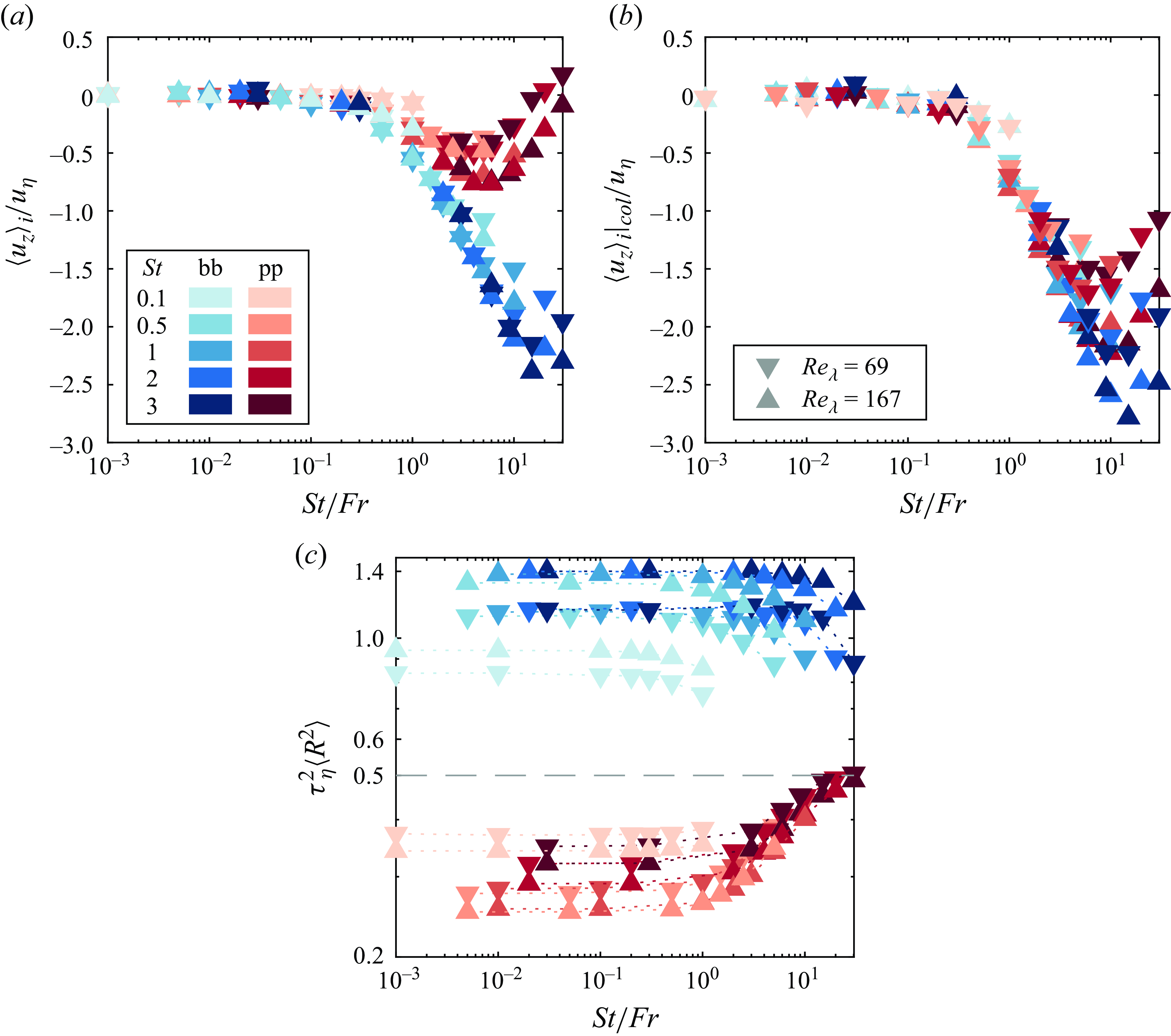
Figure 4. (a) Mean vertical fluid velocity at bubble and particle positions plotted against $St/Fr$
. (b) Same as (a) but conditioned on pairs with
$St/Fr$
. (b) Same as (a) but conditioned on pairs with $r\in [r_c-0.1\eta ,r_c + 0.1\eta ]$
. (c) The norm of the rotation rate of the flow at bubble and particle positions. The lines are guides for the eye.
$r\in [r_c-0.1\eta ,r_c + 0.1\eta ]$
. (c) The norm of the rotation rate of the flow at bubble and particle positions. The lines are guides for the eye.
To directly measure the overall effect of preferential sampling on the collision kernel, we compute the RDF at collision distance $g(r_c)$
, which reflects the probability of finding a particle at a distance
$g(r_c)$
, which reflects the probability of finding a particle at a distance $r_c$
from another particle relative to a uniform distribution. In short,
$r_c$
from another particle relative to a uniform distribution. In short, $g(r_c) \lt 1$
and
$g(r_c) \lt 1$
and ${\gt } 1$
indicate segregation and clustering, which respectively either decreases or increases the collision rate based on (1.3). Figure 5(a) shows
${\gt } 1$
indicate segregation and clustering, which respectively either decreases or increases the collision rate based on (1.3). Figure 5(a) shows $g(r_c)$
as a function of
$g(r_c)$
as a function of $St/Fr$
. Focusing on the lowest
$St/Fr$
. Focusing on the lowest $1/Fr$
case when gravity is still weak, bubbles and particles form their own clusters so
$1/Fr$
case when gravity is still weak, bubbles and particles form their own clusters so $g_{bb}(r_c)$
and
$g_{bb}(r_c)$
and $g_{pp}(r_c)\gt 1$
. However, since bubbles and particles individually cluster at different regions of the flow owing to their different relative densities, they segregate and
$g_{pp}(r_c)\gt 1$
. However, since bubbles and particles individually cluster at different regions of the flow owing to their different relative densities, they segregate and $g_{bp}(r_c)\lt 1$
. The segregation is strongest at
$g_{bp}(r_c)\lt 1$
. The segregation is strongest at $St = 1$
when
$St = 1$
when $g_{bp}(r_c)$
reaches its lowest value, which is consistent with the no-gravity case (Chan et al. Reference Chan, Ng and Krug2023). As
$g_{bp}(r_c)$
reaches its lowest value, which is consistent with the no-gravity case (Chan et al. Reference Chan, Ng and Krug2023). As $1/Fr$
increases, the extent of segregation reduces and eventually reaches
$1/Fr$
increases, the extent of segregation reduces and eventually reaches $g_{bp}(r_c) = 1$
. We note that
$g_{bp}(r_c) = 1$
. We note that $g_{bp}(r_c)$
for
$g_{bp}(r_c)$
for $St \geqslant 0.5$
collapses when plotted against
$St \geqslant 0.5$
collapses when plotted against $St/Fr$
as shown in figure 5(a). This may be because particle clusters are affected by preferential sampling (Wang & Maxey Reference Wang and Maxey1993), which scales as
$St/Fr$
as shown in figure 5(a). This may be because particle clusters are affected by preferential sampling (Wang & Maxey Reference Wang and Maxey1993), which scales as $St/Fr$
as shown in figure 4(a). Curiously, neither
$St/Fr$
as shown in figure 4(a). Curiously, neither $g_{bb}(r_c)$
nor
$g_{bb}(r_c)$
nor $g_{pp}(r_c)$
reaches 1 even at the largest tested value of
$g_{pp}(r_c)$
reaches 1 even at the largest tested value of $St/Fr$
, which indicates that reduced bubble or particle clustering is not the primary cause of the reduced segregation. On closer inspection,
$St/Fr$
, which indicates that reduced bubble or particle clustering is not the primary cause of the reduced segregation. On closer inspection, $g_{bp}(r_c)$
for
$g_{bp}(r_c)$
for $St \geqslant 0.5$
already deviates noticeably from the
$St \geqslant 0.5$
already deviates noticeably from the $1/Fr \rightarrow 0$
limit in the range
$1/Fr \rightarrow 0$
limit in the range $10^{-1} \lesssim St/Fr \lesssim 10^{0}$
despite
$10^{-1} \lesssim St/Fr \lesssim 10^{0}$
despite $g_{pp}(r_c)$
and
$g_{pp}(r_c)$
and $g_{bb}(r_c)$
remaining mostly constant, i.e. bubbles and particles still cluster as strongly as before. From figure 4(c), in this range of
$g_{bb}(r_c)$
remaining mostly constant, i.e. bubbles and particles still cluster as strongly as before. From figure 4(c), in this range of $St/Fr$
, the value of the bubble
$St/Fr$
, the value of the bubble $\langle R^2 \rangle$
already decreases for
$\langle R^2 \rangle$
already decreases for $St = 0.5$
and the value of the particle
$St = 0.5$
and the value of the particle $\langle R^2 \rangle$
already increases for
$\langle R^2 \rangle$
already increases for $St \geqslant 1$
. This suggests the bubbles and particle clusters migrate closer together, which would increase
$St \geqslant 1$
. This suggests the bubbles and particle clusters migrate closer together, which would increase $g_{bp}(r_c)$
. For the tested parameters,
$g_{bp}(r_c)$
. For the tested parameters, $g_{bp}(r_c)$
is not sensitive to
$g_{bp}(r_c)$
is not sensitive to $Re_\lambda$
. To account for segregation in the model by Dodin & Elperin (Reference Dodin and Elperin2002), we multiply
$Re_\lambda$
. To account for segregation in the model by Dodin & Elperin (Reference Dodin and Elperin2002), we multiply $g_{bp}(r_c)$
to
$g_{bp}(r_c)$
to $\Gamma ^{(DEX)}$
to obtain
$\Gamma ^{(DEX)}$
to obtain $\Gamma ^{(DEXc)}$
, which is plotted in figure 5(b). As anticipated,
$\Gamma ^{(DEXc)}$
, which is plotted in figure 5(b). As anticipated, $\Gamma ^{(DEXc)}$
agrees excellently with the simulation data at the lowest
$\Gamma ^{(DEXc)}$
agrees excellently with the simulation data at the lowest $St$
, indicating that the model correctly represents the relevant physics when corrected for the effect of segregation.
$St$
, indicating that the model correctly represents the relevant physics when corrected for the effect of segregation.

Figure 5. (a) The RDF at collision distance $g(r_c)$
. Only 25 % of all the bubbles were considered when computing
$g(r_c)$
. Only 25 % of all the bubbles were considered when computing $g_{bb}(r_c)$
. (b) The collision kernel and the prediction of the extended Dodin & Elperin (Reference Dodin and Elperin2002) model after compensating for
$g_{bb}(r_c)$
. (b) The collision kernel and the prediction of the extended Dodin & Elperin (Reference Dodin and Elperin2002) model after compensating for $g(r_c)$
plotted against
$g(r_c)$
plotted against $1/Fr$
for
$1/Fr$
for $Re_\lambda = 167$
. The lines are guides for the eye. The symbols and colour scheme follow figures 2 and 4.
$Re_\lambda = 167$
. The lines are guides for the eye. The symbols and colour scheme follow figures 2 and 4.
As gravity introduces anisotropy in the vertical direction, we further quantitatively examine the bubble–particle spatial distribution by binning the RDF by the polar angle to obtain the angular distribution function (ADF) (Gualtieri, Picano & Casciola Reference Gualtieri, Picano and Casciola2009; Ireland et al. Reference Ireland, Bragg and Collins2016b
), which is normalised by the RDF in figure 6. We have ADF $/g_{bp}(r) \neq 1$
everywhere when gravity is included, as expected (Ireland et al. Reference Ireland, Bragg and Collins2016b
). Intriguingly, particles preferentially sample the regions directly above bubbles, especially when
$/g_{bp}(r) \neq 1$
everywhere when gravity is included, as expected (Ireland et al. Reference Ireland, Bragg and Collins2016b
). Intriguingly, particles preferentially sample the regions directly above bubbles, especially when $St/Fr$
becomes sufficiently large. To understand this, we consider figure 4(a), which showed that bubbles and particles preferentially sample downflows, and examine the local flow structure by overlaying the ADF on top of the azimuthally averaged flow field around the bubble in a reference frame where the mean vertical flow velocity in the sampled region is zero in figure 6. The results show that there are vortices with their downward branches passing the bubble and the region where the flow converges horizontally corresponds to the locations with higher particle concentration, suggesting that the convergent flow influences the particle trajectories such that they are concentrated above bubbles. In the cases with appreciable anisotropic particle distributions (i.e.
$St/Fr$
becomes sufficiently large. To understand this, we consider figure 4(a), which showed that bubbles and particles preferentially sample downflows, and examine the local flow structure by overlaying the ADF on top of the azimuthally averaged flow field around the bubble in a reference frame where the mean vertical flow velocity in the sampled region is zero in figure 6. The results show that there are vortices with their downward branches passing the bubble and the region where the flow converges horizontally corresponds to the locations with higher particle concentration, suggesting that the convergent flow influences the particle trajectories such that they are concentrated above bubbles. In the cases with appreciable anisotropic particle distributions (i.e. $St = 1,3$
and
$St = 1,3$
and $1/Fr \geqslant 1$
), the vertical component of the flow velocity vector at the bubble position, as displayed in figure 6, amounts to 60 %–80 % of
$1/Fr \geqslant 1$
), the vertical component of the flow velocity vector at the bubble position, as displayed in figure 6, amounts to 60 %–80 % of $\langle u_z \rangle _b$
and decreases very slightly as
$\langle u_z \rangle _b$
and decreases very slightly as $1/Fr$
increases. Despite the local flow field contributing less to
$1/Fr$
increases. Despite the local flow field contributing less to $\langle u_z \rangle _b$
with increasing
$\langle u_z \rangle _b$
with increasing $1/Fr$
, the particle distribution is most anisotropic at intermediate
$1/Fr$
, the particle distribution is most anisotropic at intermediate $1/Fr$
since the particles settle faster at large
$1/Fr$
since the particles settle faster at large $1/Fr$
, meaning they will have less time to interact with the background turbulence such that they will be more isotropically distributed. For the tested parameters, this anisotropy increases with
$1/Fr$
, meaning they will have less time to interact with the background turbulence such that they will be more isotropically distributed. For the tested parameters, this anisotropy increases with $St$
. Nonetheless, we expect that it is strongest for some finite
$St$
. Nonetheless, we expect that it is strongest for some finite $St$
and weakens as
$St$
and weakens as $St$
becomes very large when the particles no longer respond to the background flow. Overall, this means that collisions will occur more frequently on top of a bubble at intermediate
$St$
becomes very large when the particles no longer respond to the background flow. Overall, this means that collisions will occur more frequently on top of a bubble at intermediate $1/Fr$
and
$1/Fr$
and $St$
even without considering the azimuthal variation of the collision velocity due to gravity.
$St$
even without considering the azimuthal variation of the collision velocity due to gravity.
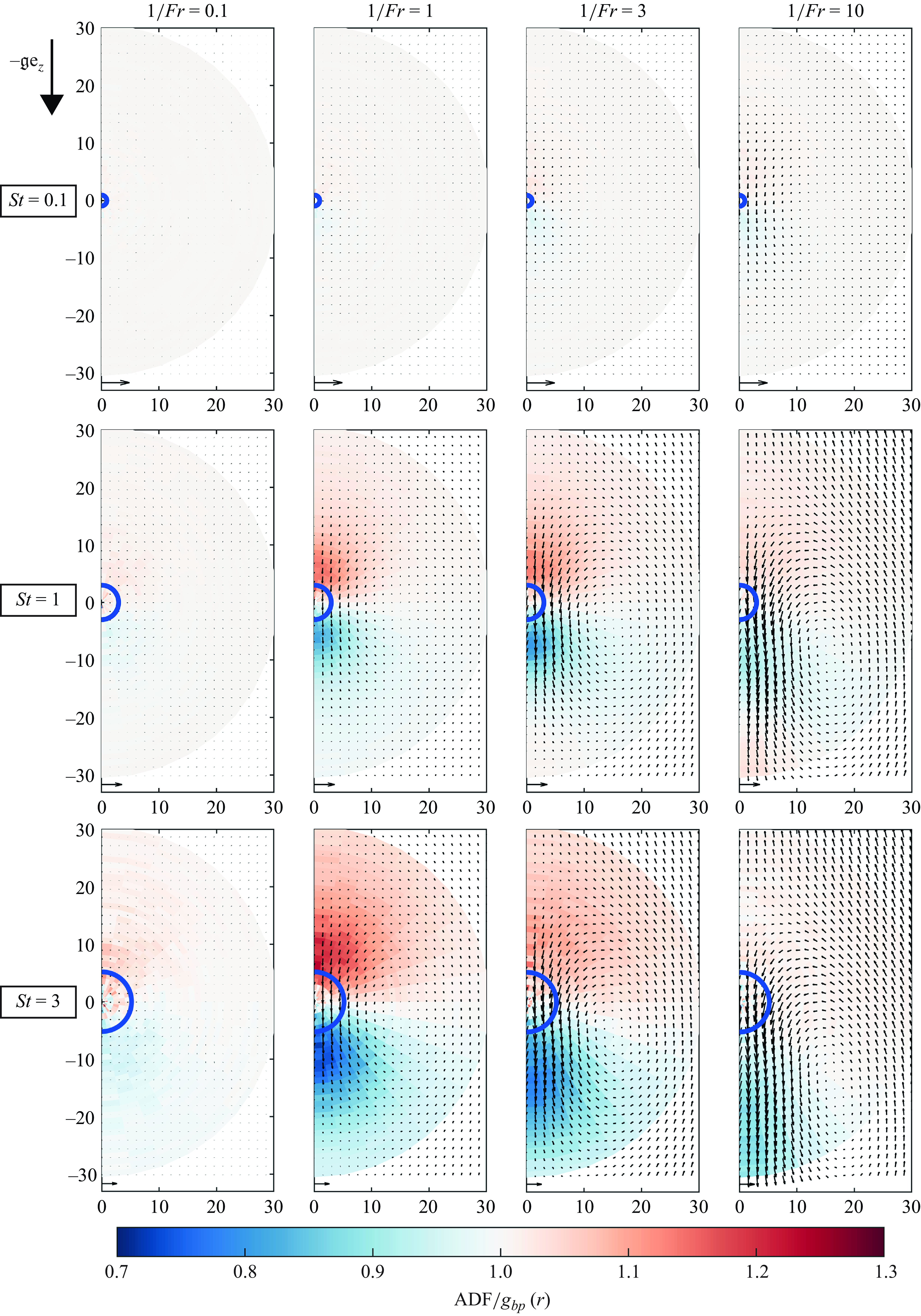
Figure 6. The ADF at different distances and the azimuthally averaged local flow field in a reference frame where the mean vertical flow velocity in the sampled region is zero. Here, $Re_\lambda = 167$
. The semicircle and the reference arrow on the bottom row indicate the bubble and
$Re_\lambda = 167$
. The semicircle and the reference arrow on the bottom row indicate the bubble and $u_\eta$
, respectively. The axis labels are in units of
$u_\eta$
, respectively. The axis labels are in units of $\eta$
.
$\eta$
.

Figure 7. (a) Value of $S_-(r_c)$
at different
$S_-(r_c)$
at different $1/Fr$
. The model predictions are displayed only for
$1/Fr$
. The model predictions are displayed only for $Re_\lambda = 167$
. The colour scheme and symbols follow figure 2(a). (b) The non-dimensionalised distribution of
$Re_\lambda = 167$
. The colour scheme and symbols follow figure 2(a). (b) The non-dimensionalised distribution of $S_{\theta -}$
along the polar angle
$S_{\theta -}$
along the polar angle $\theta$
for
$\theta$
for $Re_\lambda = 167$
. The colour scheme follows figure 2(a).
$Re_\lambda = 167$
. The colour scheme follows figure 2(a).
4.3. Collision velocity
Besides the bubble–particle distribution, the collision kernel is determined by the effective radial approach velocity at collision distance $S_-(r_c)$
according to (1.3). Figure 7(a) shows
$S_-(r_c)$
according to (1.3). Figure 7(a) shows $S_-(r_c)$
as a function of
$S_-(r_c)$
as a function of $1/Fr$
. Here,
$1/Fr$
. Here, $S_-$
increases significantly with
$S_-$
increases significantly with $1/Fr$
when
$1/Fr$
when $1/Fr \gt 1$
for all
$1/Fr \gt 1$
for all $St$
and almost recovers the relative settling limit
$St$
and almost recovers the relative settling limit $S_-^{(G)}$
at
$S_-^{(G)}$
at $1/Fr \sim 10$
– a point which we will return to. At low
$1/Fr \sim 10$
– a point which we will return to. At low $1/Fr$
where turbulence dominates,
$1/Fr$
where turbulence dominates, $S_-$
differs across
$S_-$
differs across $St$
because of the different collision mechanisms involved. At small
$St$
because of the different collision mechanisms involved. At small $St$
, collisions occur due to local fluid shear and the local turnstile effect, as introduced in § 1. As
$St$
, collisions occur due to local fluid shear and the local turnstile effect, as introduced in § 1. As $St$
increases, local effects become less important since the bubbles and particles interact with larger and more energetic eddies. Due to the different physical properties of bubbles and particles, the interaction is different between bubbles and particles, which contributes to
$St$
increases, local effects become less important since the bubbles and particles interact with larger and more energetic eddies. Due to the different physical properties of bubbles and particles, the interaction is different between bubbles and particles, which contributes to $S_-$
, i.e. the ‘non-local turnstile effect’. The local shear and local turnstile effects, as well as the relative settling effect of gravity, are properly represented in the extended Dodin & Elperin (Reference Dodin and Elperin2002) prediction
$S_-$
, i.e. the ‘non-local turnstile effect’. The local shear and local turnstile effects, as well as the relative settling effect of gravity, are properly represented in the extended Dodin & Elperin (Reference Dodin and Elperin2002) prediction $S_-^{(DEX)}$
, which explains its excellent agreement with the data throughout the entire
$S_-^{(DEX)}$
, which explains its excellent agreement with the data throughout the entire $1/Fr$
range at
$1/Fr$
range at $St = 0.1$
. However, it increasingly overpredicts
$St = 0.1$
. However, it increasingly overpredicts $S_-$
at larger
$S_-$
at larger $St$
as it does not model any non-local effects. These non-local effects do not directly increase
$St$
as it does not model any non-local effects. These non-local effects do not directly increase $S_-$
by improving the alignment between the relative velocity vector and the separation vector, in contrast to the local turnstile effect. Considering only local effects at higher
$S_-$
by improving the alignment between the relative velocity vector and the separation vector, in contrast to the local turnstile effect. Considering only local effects at higher $St$
regimes can therefore lead to the overprediction. At higher
$St$
regimes can therefore lead to the overprediction. At higher $1/Fr$
, the overprediction decreases since the contribution of the turbulence collision mechanisms decreases and relative settling plays an increasingly dominant role. Another approach to quantify the gravity effect is to consider the angular distribution of
$1/Fr$
, the overprediction decreases since the contribution of the turbulence collision mechanisms decreases and relative settling plays an increasingly dominant role. Another approach to quantify the gravity effect is to consider the angular distribution of $S_-(r_c)$
with respect to gravity, where
$S_-(r_c)$
with respect to gravity, where $S_{-}(r_c)$
is binned using the polar angle
$S_{-}(r_c)$
is binned using the polar angle $\theta$
around the bubble to obtain
$\theta$
around the bubble to obtain $S_{\theta -}$
. This is plotted in figure 7(b) with
$S_{\theta -}$
. This is plotted in figure 7(b) with $\theta = -90^\circ$
corresponding to the direction of gravity. In the no-gravity (
$\theta = -90^\circ$
corresponding to the direction of gravity. In the no-gravity ( $1/Fr = 0$
) limit, there is no preferred direction and accordingly
$1/Fr = 0$
) limit, there is no preferred direction and accordingly $S_{\theta -}$
is uniformly distributed across all
$S_{\theta -}$
is uniformly distributed across all $\theta$
(grey line). As
$\theta$
(grey line). As $1/Fr$
increases, more and more collisions occur on the top half of a bubble where the approach velocity is enhanced due to gravitational settling and vice versa for the lower half. Consequently, the top hemisphere (
$1/Fr$
increases, more and more collisions occur on the top half of a bubble where the approach velocity is enhanced due to gravitational settling and vice versa for the lower half. Consequently, the top hemisphere ( $\theta \gt 0^\circ$
) contributes more to
$\theta \gt 0^\circ$
) contributes more to $S_-(r_c)$
than the bottom one. This anisotropy is still very weak at
$S_-(r_c)$
than the bottom one. This anisotropy is still very weak at $1/Fr = 0.1$
and becomes significant at
$1/Fr = 0.1$
and becomes significant at $1/Fr = 1$
, even though at this value
$1/Fr = 1$
, even though at this value $S_-(r_c)$
still has not increased significantly from the turbulence-dominated limit, as shown in figure 7(a). At
$S_-(r_c)$
still has not increased significantly from the turbulence-dominated limit, as shown in figure 7(a). At $1/Fr = 10$
, only a small fraction of the collisions occur in the bottom hemisphere due to turbulence, and the distribution is close to the relative settling limit (purple line) where collisions exclusively occur on the top hemisphere. Furthermore, in the range
$1/Fr = 10$
, only a small fraction of the collisions occur in the bottom hemisphere due to turbulence, and the distribution is close to the relative settling limit (purple line) where collisions exclusively occur on the top hemisphere. Furthermore, in the range $1\leqslant 1/Fr\lt 10$
,
$1\leqslant 1/Fr\lt 10$
, $S_{\theta -}$
is not sensitive to
$S_{\theta -}$
is not sensitive to $St$
for
$St$
for $St \geqslant 0.5$
, suggesting the transition from turbulence to relative settling for the collision velocity is similar at different values of
$St \geqslant 0.5$
, suggesting the transition from turbulence to relative settling for the collision velocity is similar at different values of $St$
.
$St$
.
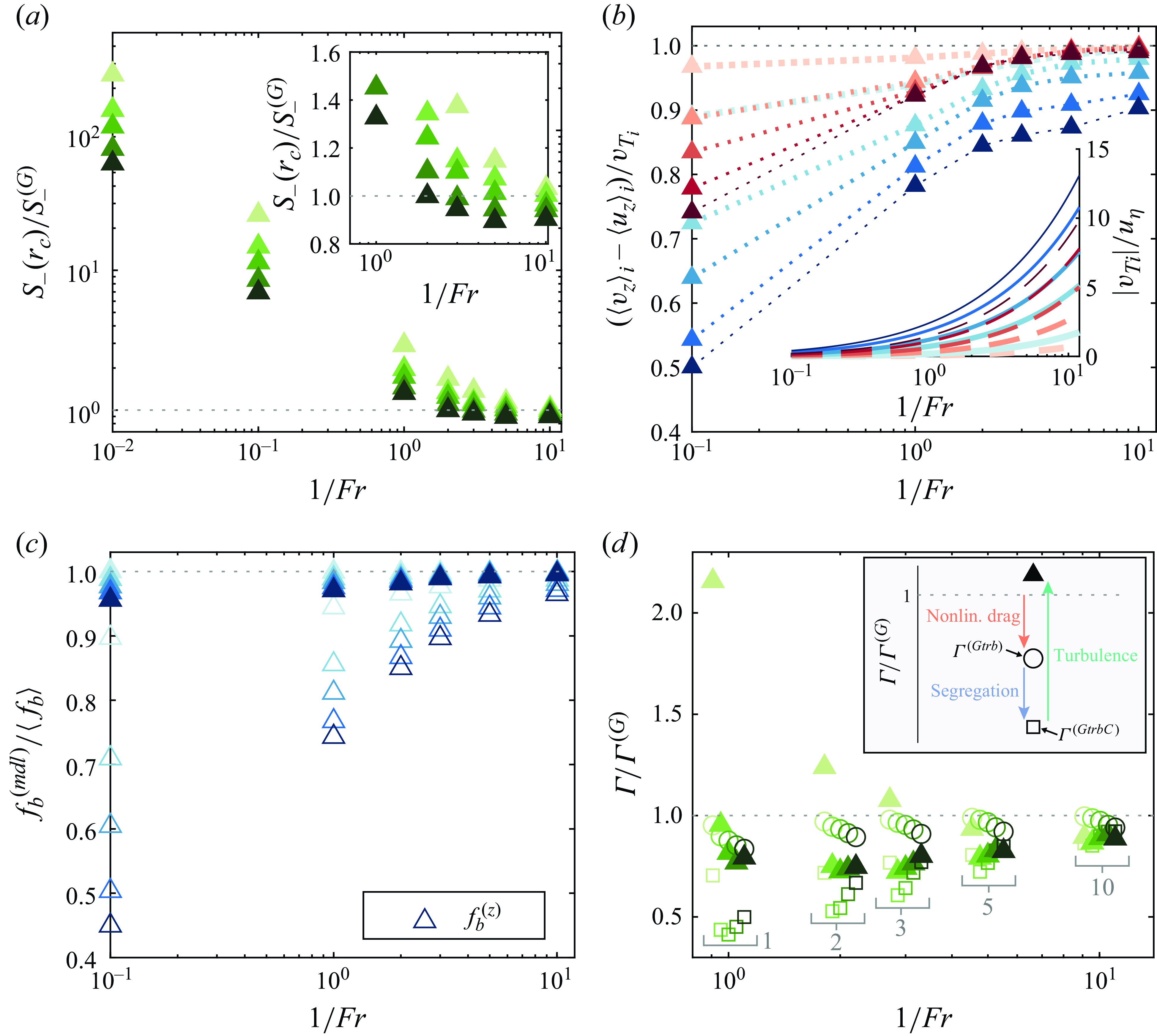
Figure 8. (a) The ratio of $S_-(r_c)$
to the relative settling case
$S_-(r_c)$
to the relative settling case $S_-^{(G)}$
at
$S_-^{(G)}$
at $Re_\lambda = 167$
. Inset shows an enlarged version of the region where
$Re_\lambda = 167$
. Inset shows an enlarged version of the region where $S_-(r_c) \lt S_-^{(G)}$
. (b) The ratio of the average bubble and particle vertical slip velocity to the terminal velocity in still fluid accounting for nonlinear drag
$S_-(r_c) \lt S_-^{(G)}$
. (b) The ratio of the average bubble and particle vertical slip velocity to the terminal velocity in still fluid accounting for nonlinear drag $v_{Ti}$
, whose magnitude is shown in the inset (solid line for bubbles and dashed lines for particles), at
$v_{Ti}$
, whose magnitude is shown in the inset (solid line for bubbles and dashed lines for particles), at $Re_\lambda = 167$
. The lines in the main figure are guides for the eye. (c) The ratio of the modelled drag correction to the measured drag correction at
$Re_\lambda = 167$
. The lines in the main figure are guides for the eye. (c) The ratio of the modelled drag correction to the measured drag correction at $Re_\lambda = 167$
. The open symbols indicate the drag correction based solely on the vertical slip velocity. (d) The collision kernel normalised by the relative settling case in still fluid at
$Re_\lambda = 167$
. The open symbols indicate the drag correction based solely on the vertical slip velocity. (d) The collision kernel normalised by the relative settling case in still fluid at $Re_\lambda = 167$
. Also shown are the relative settling collision kernel in turbulence
$Re_\lambda = 167$
. Also shown are the relative settling collision kernel in turbulence $\Gamma ^{(Gtrb)}$
and the effect of segregation. The cases with different
$\Gamma ^{(Gtrb)}$
and the effect of segregation. The cases with different $St$
have been laterally displaced for clarity and the associated labels indicate the corresponding
$St$
have been laterally displaced for clarity and the associated labels indicate the corresponding $1/Fr$
. The symbols and the colour scheme in all the panels follow figures 2(a) and 4(a).
$1/Fr$
. The symbols and the colour scheme in all the panels follow figures 2(a) and 4(a).
Similar to our analysis of the collision kernel, we normalise $S_-(r_c)$
with the relative settling case in still fluid
$S_-(r_c)$
with the relative settling case in still fluid $S_-^{(G)} = (|v_{Tb}| + |v_{Tp}|)/4$
, where
$S_-^{(G)} = (|v_{Tb}| + |v_{Tp}|)/4$
, where $v_{Ti}$
are the terminal velocities obtained by balancing the drag and buoyancy terms in (3.2) taking
$v_{Ti}$
are the terminal velocities obtained by balancing the drag and buoyancy terms in (3.2) taking $\boldsymbol{u} = \boldsymbol{0}$
, and plot the result in figure 8(a). Although we only show the data for the
$\boldsymbol{u} = \boldsymbol{0}$
, and plot the result in figure 8(a). Although we only show the data for the $Re_\lambda = 167$
case, the results are not sensitive to
$Re_\lambda = 167$
case, the results are not sensitive to $Re_\lambda$
so the following discussion also applies to
$Re_\lambda$
so the following discussion also applies to $Re_\lambda = 69$
. Generally,
$Re_\lambda = 69$
. Generally, $S_-(r_c)/S_-^{(G)}$
decreases as
$S_-(r_c)/S_-^{(G)}$
decreases as $1/Fr$
increases, reflecting the growing contribution of gravity. Upon closer inspection, we observe that
$1/Fr$
increases, reflecting the growing contribution of gravity. Upon closer inspection, we observe that $S_-(r_c)$
for
$S_-(r_c)$
for $St \gt 0.5$
dips below
$St \gt 0.5$
dips below $S_-^{(G)}$
, instead of simply approaching
$S_-^{(G)}$
, instead of simply approaching $S_-^{(G)}$
as is the case for
$S_-^{(G)}$
as is the case for $St = 0.1$
. Note that this is not due to preferential sampling as the fluid velocities sampled by the colliding bubbles and particles are almost the same, as already shown in figure 4(b). To investigate why
$St = 0.1$
. Note that this is not due to preferential sampling as the fluid velocities sampled by the colliding bubbles and particles are almost the same, as already shown in figure 4(b). To investigate why $S_- \lt S_-^{(G)}$
, we compare the mean vertical slip velocity of the bubbles and particles
$S_- \lt S_-^{(G)}$
, we compare the mean vertical slip velocity of the bubbles and particles $\langle v_z \rangle _i - \langle u_z \rangle _i$
with the theoretical terminal velocity in still fluid
$\langle v_z \rangle _i - \langle u_z \rangle _i$
with the theoretical terminal velocity in still fluid $v_{Ti}$
, on which
$v_{Ti}$
, on which $S_-^{(G)}$
in figure 8(b) is based. For
$S_-^{(G)}$
in figure 8(b) is based. For $St = 0.1$
,
$St = 0.1$
, $(\langle v_z \rangle _i - \langle u_z \rangle _i)/v_{Ti}$
is very close to 1 throughout, which is consistent with the fact that
$(\langle v_z \rangle _i - \langle u_z \rangle _i)/v_{Ti}$
is very close to 1 throughout, which is consistent with the fact that $S_- \geqslant S_-^{(G)}$
. For higher
$S_- \geqslant S_-^{(G)}$
. For higher $St$
, however, the mean vertical slip velocity in turbulence is smaller than
$St$
, however, the mean vertical slip velocity in turbulence is smaller than $v_{Ti}$
. This effect is generally stronger for bubbles, more pronounced at high
$v_{Ti}$
. This effect is generally stronger for bubbles, more pronounced at high $St$
and overall the ratio
$St$
and overall the ratio $(\langle v_z \rangle _i - \langle u_z \rangle _i)/v_{Ti}$
trends back up towards 1 as buoyancy becomes stronger. To understand its origin, we focus on the bubbles and consider the fact that turbulence induces additional horizontal slip velocities. As
$(\langle v_z \rangle _i - \langle u_z \rangle _i)/v_{Ti}$
trends back up towards 1 as buoyancy becomes stronger. To understand its origin, we focus on the bubbles and consider the fact that turbulence induces additional horizontal slip velocities. As $Re_i$
depends on magnitude of the total slip velocity, the horizontal slip increases the value of
$Re_i$
depends on magnitude of the total slip velocity, the horizontal slip increases the value of $Re_i$
and the drag force, which can explain the slowdown (Ruth et al. Reference Ruth, Vernet, Perrard and Deike2021). To test this hypothesis, we model the slip velocity vector as
$Re_i$
and the drag force, which can explain the slowdown (Ruth et al. Reference Ruth, Vernet, Perrard and Deike2021). To test this hypothesis, we model the slip velocity vector as $(\boldsymbol{v_b}-\boldsymbol{u})^{(mdl)} = (v_{bx} - u_{bx})'\boldsymbol{e_x} + (v_{bx} - u_{bx})'\boldsymbol{e_y} + (\langle v_z\rangle _b - \langle u_z\rangle _b)\boldsymbol{e_z}$
, where
$(\boldsymbol{v_b}-\boldsymbol{u})^{(mdl)} = (v_{bx} - u_{bx})'\boldsymbol{e_x} + (v_{bx} - u_{bx})'\boldsymbol{e_y} + (\langle v_z\rangle _b - \langle u_z\rangle _b)\boldsymbol{e_z}$
, where $(v_{bx} - u_{bx})'$
is the measured r.m.s. of the horizontal bubble slip velocity and
$(v_{bx} - u_{bx})'$
is the measured r.m.s. of the horizontal bubble slip velocity and $\boldsymbol{e_{x,y,z}}$
are unit vectors along
$\boldsymbol{e_{x,y,z}}$
are unit vectors along $x$
-,
$x$
-, $y$
- and the vertical directions, respectively. Based on the magnitude of the slip velocity vector, we then calculate the resulting
$y$
- and the vertical directions, respectively. Based on the magnitude of the slip velocity vector, we then calculate the resulting $Re_i$
and the corresponding drag correction term
$Re_i$
and the corresponding drag correction term $f_b^{(mdl)}$
. Figure 8(c) shows that
$f_b^{(mdl)}$
. Figure 8(c) shows that $f_b^{(mdl)}$
is indeed close to the measured mean drag correction
$f_b^{(mdl)}$
is indeed close to the measured mean drag correction $\langle f_b \rangle$
. For reference, we also include the drag correction based on the vertical slip velocity only
$\langle f_b \rangle$
. For reference, we also include the drag correction based on the vertical slip velocity only $(\boldsymbol{v_b}-\boldsymbol{u})^{(z)}=(\langle v_z\rangle _b - \langle u_z\rangle _b)\boldsymbol{e_z}$
as open symbols. As expected,
$(\boldsymbol{v_b}-\boldsymbol{u})^{(z)}=(\langle v_z\rangle _b - \langle u_z\rangle _b)\boldsymbol{e_z}$
as open symbols. As expected, $f_b^{(z)} \lt f_b^{(mdl)}$
and the difference reduces at larger
$f_b^{(z)} \lt f_b^{(mdl)}$
and the difference reduces at larger $1/Fr$
, consistent with the trend of
$1/Fr$
, consistent with the trend of $(\langle v_z \rangle _b - \langle u_z \rangle _b)/v_{Tb}$
in figure 8(b). This is because the mean vertical slip velocity becomes larger relative to the horizontal slip velocities with increasing
$(\langle v_z \rangle _b - \langle u_z \rangle _b)/v_{Tb}$
in figure 8(b). This is because the mean vertical slip velocity becomes larger relative to the horizontal slip velocities with increasing $1/Fr$
, such that
$1/Fr$
, such that $|\langle v_z\rangle _b - \langle u_z\rangle _b|$
increasingly dominates
$|\langle v_z\rangle _b - \langle u_z\rangle _b|$
increasingly dominates $|\boldsymbol{v_b}-\boldsymbol{u}|$
. We therefore conclude that the observed reduction in the rise velocity is indeed due to enhanced nonlinear drag caused by the horizontal slip velocity components in turbulence.
$|\boldsymbol{v_b}-\boldsymbol{u}|$
. We therefore conclude that the observed reduction in the rise velocity is indeed due to enhanced nonlinear drag caused by the horizontal slip velocity components in turbulence.
Combining these insights, we re-examine the unexpected result that turbulence can reduce the collision rate (i.e. $\Gamma \lt \Gamma ^{(G)}$
), as seen in figure 2(a). Our analysis shows that this can be attributed to bubble–particle spatial segregation and the reduced bubble slip velocity in turbulence. To evaluate their respective importance, we again show
$\Gamma \lt \Gamma ^{(G)}$
), as seen in figure 2(a). Our analysis shows that this can be attributed to bubble–particle spatial segregation and the reduced bubble slip velocity in turbulence. To evaluate their respective importance, we again show $\Gamma /\Gamma ^{(G)}$
in figure 8(d), this time focusing only on the parameter range where
$\Gamma /\Gamma ^{(G)}$
in figure 8(d), this time focusing only on the parameter range where $\Gamma \lt \Gamma ^{(G)}$
. To quantify the effect of the nonlinear drag, we plot the relative settling collision kernel in turbulence
$\Gamma \lt \Gamma ^{(G)}$
. To quantify the effect of the nonlinear drag, we plot the relative settling collision kernel in turbulence $\Gamma ^{(Gtrb)} = \pi r_c^2 [\langle v_{z} \rangle _b - \langle u_{z} \rangle _b - (\langle v_{z} \rangle _p - \langle u_{z} \rangle _p)]$
, i.e. based on the measured vertical slip velocities of bubbles and particles. Here,
$\Gamma ^{(Gtrb)} = \pi r_c^2 [\langle v_{z} \rangle _b - \langle u_{z} \rangle _b - (\langle v_{z} \rangle _p - \langle u_{z} \rangle _p)]$
, i.e. based on the measured vertical slip velocities of bubbles and particles. Here, $\Gamma ^{(Gtrb)}/\Gamma ^{(G)}\leqslant 1$
as the nonlinear drag reduces the bubble slip velocity. As
$\Gamma ^{(Gtrb)}/\Gamma ^{(G)}\leqslant 1$
as the nonlinear drag reduces the bubble slip velocity. As $1/Fr$
increases,
$1/Fr$
increases, $\Gamma ^{(Gtrb)}/\Gamma ^{(G)}$
increases since the magnitude of the slip velocity is increasingly dominated by the vertical component, whereas
$\Gamma ^{(Gtrb)}/\Gamma ^{(G)}$
increases since the magnitude of the slip velocity is increasingly dominated by the vertical component, whereas $\Gamma ^{(Gtrb)}/\Gamma ^{(G)}$
decreases for increasing
$\Gamma ^{(Gtrb)}/\Gamma ^{(G)}$
decreases for increasing $St$
as the effect of nonlinear drag becomes more pronounced. Since bubbles and particles segregate in turbulence, we also show
$St$
as the effect of nonlinear drag becomes more pronounced. Since bubbles and particles segregate in turbulence, we also show $\Gamma ^{(GtrbC)} = \Gamma ^{(Gtrb)}\cdot g(r_c)$
in the figure. The difference between
$\Gamma ^{(GtrbC)} = \Gamma ^{(Gtrb)}\cdot g(r_c)$
in the figure. The difference between $\Gamma ^{(GtrbC)}$
and
$\Gamma ^{(GtrbC)}$
and $\Gamma ^{(Gtrb)}$
decreases with increasing
$\Gamma ^{(Gtrb)}$
decreases with increasing $1/Fr$
, reflecting the fact that gravity reduces segregation. Finally, the difference between
$1/Fr$
, reflecting the fact that gravity reduces segregation. Finally, the difference between $\Gamma ^{(GtrbC)}$
and
$\Gamma ^{(GtrbC)}$
and $\Gamma$
indicates the enhancement of the collision velocity due to turbulence mechanisms. This is larger at lower
$\Gamma$
indicates the enhancement of the collision velocity due to turbulence mechanisms. This is larger at lower $1/Fr$
and by
$1/Fr$
and by $1/Fr = 10$
,
$1/Fr = 10$
, $\Gamma \approx \Gamma ^{(GtrbC)}$
.
$\Gamma \approx \Gamma ^{(GtrbC)}$
.
4.4. Effect of the particle density
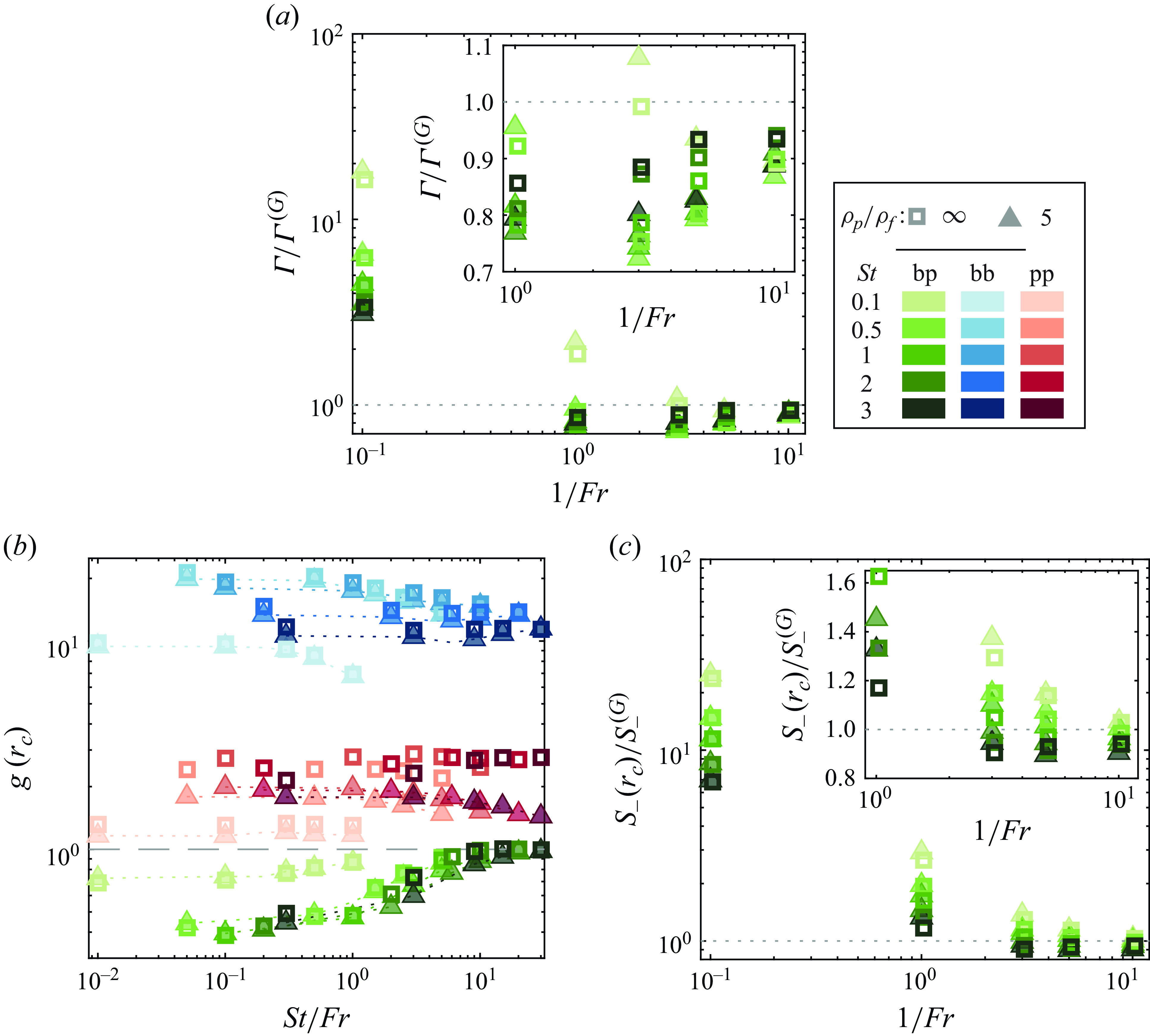
Figure 9. (a) The collision kernel $\Gamma$
normalised by the relative settling limit, (b) the RDF
$\Gamma$
normalised by the relative settling limit, (b) the RDF $g(r_c)$
and (c)
$g(r_c)$
and (c) $S_-(r_c)$
normalised by the relative settling limit for both
$S_-(r_c)$
normalised by the relative settling limit for both $\rho _p/\rho _b = 5$
(filled triangles) and
$\rho _p/\rho _b = 5$
(filled triangles) and $\rho _p/\rho _b =\infty$
(open squares) at
$\rho _p/\rho _b =\infty$
(open squares) at $Re_\lambda = 167$
. The insets in (a) and (c) are zooms in on the
$Re_\lambda = 167$
. The insets in (a) and (c) are zooms in on the $1 \lesssim 1/Fr \lesssim 10$
region.
$1 \lesssim 1/Fr \lesssim 10$
region.
In the previous sections, we fixed $\rho _p/\rho _f = 5$
and varied
$\rho _p/\rho _f = 5$
and varied $St$
and
$St$
and $1/Fr$
. Nevertheless,
$1/Fr$
. Nevertheless, $\rho _p/\rho _f$
, which sets
$\rho _p/\rho _f$
, which sets $r_p$
hence
$r_p$
hence $r_c$
, can have an explicit effect on the particle dynamics beyond determining the collision distance according to (3.2). We therefore additionally simulate
$r_c$
, can have an explicit effect on the particle dynamics beyond determining the collision distance according to (3.2). We therefore additionally simulate $\rho _p/\rho _f = \infty$
with
$\rho _p/\rho _f = \infty$
with $1/Fr = 0.1,1,3,5$
and 10 for all the tested values of
$1/Fr = 0.1,1,3,5$
and 10 for all the tested values of $St$
at
$St$
at $Re_\lambda = 167$
, while retaining the same
$Re_\lambda = 167$
, while retaining the same $r_c$
as the
$r_c$
as the $\rho _p/\rho _f=5$
case. Figure 9 plots the collision kernel
$\rho _p/\rho _f=5$
case. Figure 9 plots the collision kernel $\Gamma$
, the RDF
$\Gamma$
, the RDF $g(r_c)$
and the effective radial approach velocity
$g(r_c)$
and the effective radial approach velocity $S_-(r_c)$
, in which
$S_-(r_c)$
, in which $\Gamma$
and
$\Gamma$
and $S_-(r_c)$
have been normalised by the relative settling limit to account for the different particle settling velocities. These data show that for the bubble–particle case neither the overall collision kernel
$S_-(r_c)$
have been normalised by the relative settling limit to account for the different particle settling velocities. These data show that for the bubble–particle case neither the overall collision kernel $\Gamma /\Gamma ^{(G)}$
, nor the factors
$\Gamma /\Gamma ^{(G)}$
, nor the factors $g_{bp}(r_c)$
and
$g_{bp}(r_c)$
and $S_-(r_c)/S_-^{(G)}$
, individually are sensitive to
$S_-(r_c)/S_-^{(G)}$
, individually are sensitive to $\rho _p$
. This is in contrast to the particle–particle case where
$\rho _p$
. This is in contrast to the particle–particle case where $g_{pp}(r_c)$
remains constant or even increases slightly with
$g_{pp}(r_c)$
remains constant or even increases slightly with $1/Fr$
, which is shown in figure 9(b) and is also observed by Woittiez et al. (Reference Woittiez, Jonker and Portela2009). Despite
$1/Fr$
, which is shown in figure 9(b) and is also observed by Woittiez et al. (Reference Woittiez, Jonker and Portela2009). Despite $g_{pp}(r_c)$
remaining above 1,
$g_{pp}(r_c)$
remaining above 1, $g_{bp}(r_c)$
approaches unity similar to the
$g_{bp}(r_c)$
approaches unity similar to the $\rho _p/\rho _f = 5$
case, which is consistent with our interpretation of figure 5(a) in § 4.2 that the trend in
$\rho _p/\rho _f = 5$
case, which is consistent with our interpretation of figure 5(a) in § 4.2 that the trend in $g_{bp}(r_c)$
with
$g_{bp}(r_c)$
with $1/Fr$
is not principally due to a change in bubble or particle clustering strength. We furthermore note that, even for
$1/Fr$
is not principally due to a change in bubble or particle clustering strength. We furthermore note that, even for $\rho _p/\rho _f = \infty$
,
$\rho _p/\rho _f = \infty$
, $S_-(r_c) \lt S_-^{(G)}$
and
$S_-(r_c) \lt S_-^{(G)}$
and $\Gamma \lt \Gamma ^{(G)}$
at intermediate values of
$\Gamma \lt \Gamma ^{(G)}$
at intermediate values of $1/Fr$
. This demonstrates that the reduction of the bubble–particle collision rate below the pure gravity case by turbulence is not specific to particles with
$1/Fr$
. This demonstrates that the reduction of the bubble–particle collision rate below the pure gravity case by turbulence is not specific to particles with $\rho _p/\rho _f = 5$
.
$\rho _p/\rho _f = 5$
.
4.5. Effect of the history force
In addition to testing $\rho _p/\rho _f = \infty$
, we examine the effect of the history force by including (3.3) in (3.2) and simulating
$\rho _p/\rho _f = \infty$
, we examine the effect of the history force by including (3.3) in (3.2) and simulating $St = 0.1,1$
and 3 for
$St = 0.1,1$
and 3 for $1/Fr = 0.1,1,3,5,10$
at
$1/Fr = 0.1,1,3,5,10$
at $Re_\lambda = 167$
. The measured
$Re_\lambda = 167$
. The measured $\Gamma /\Gamma ^{(G)}$
,
$\Gamma /\Gamma ^{(G)}$
, $g(r_c)$
and
$g(r_c)$
and $S_-(r_c)/S_-^{(G)}$
are plotted in figure 10. These results show that the history force does not qualitatively change the bubble–particle collision statistics, insofar as the general trends with
$S_-(r_c)/S_-^{(G)}$
are plotted in figure 10. These results show that the history force does not qualitatively change the bubble–particle collision statistics, insofar as the general trends with $1/Fr$
remain the same, the reduction of
$1/Fr$
remain the same, the reduction of $\Gamma$
and
$\Gamma$
and $S_-(r_c)$
below the relative settling limit is still observed in figures 10(a) and 10(c), and
$S_-(r_c)$
below the relative settling limit is still observed in figures 10(a) and 10(c), and $g_{bp}(r_c)$
still lies below 1 at low to intermediate values of
$g_{bp}(r_c)$
still lies below 1 at low to intermediate values of $1/Fr$
, as shown by figure 10(b). Quantitatively, the history force does not significantly affect the collision kernel, since it tends to reduce
$1/Fr$
, as shown by figure 10(b). Quantitatively, the history force does not significantly affect the collision kernel, since it tends to reduce $S_-(r_c)$
and increase the value of
$S_-(r_c)$
and increase the value of $g_{bp}(r_c)$
. This increase in the value of
$g_{bp}(r_c)$
. This increase in the value of $g_{bp}(r_c)$
towards 1 corresponds to reduced bubble–particle segregation. It is hence consistent with the lower values of
$g_{bp}(r_c)$
towards 1 corresponds to reduced bubble–particle segregation. It is hence consistent with the lower values of $g_{bb}(r_c)$
and
$g_{bb}(r_c)$
and $g_{pp}(r_c)$
observed when the history force is included in figure 10(b), which indicate weaker bubble and particle clusters and have already been reported in the literature (Olivieri et al. Reference Olivieri, Picano, Sardina, Iudicone and Brandt2014; Daitche Reference Daitche2015). In summary, our results show that the history force does not play a role in determining the qualitative trends of the bubble–particle collision statistics and only a minor one for the value of the collision kernel.
$g_{pp}(r_c)$
observed when the history force is included in figure 10(b), which indicate weaker bubble and particle clusters and have already been reported in the literature (Olivieri et al. Reference Olivieri, Picano, Sardina, Iudicone and Brandt2014; Daitche Reference Daitche2015). In summary, our results show that the history force does not play a role in determining the qualitative trends of the bubble–particle collision statistics and only a minor one for the value of the collision kernel.
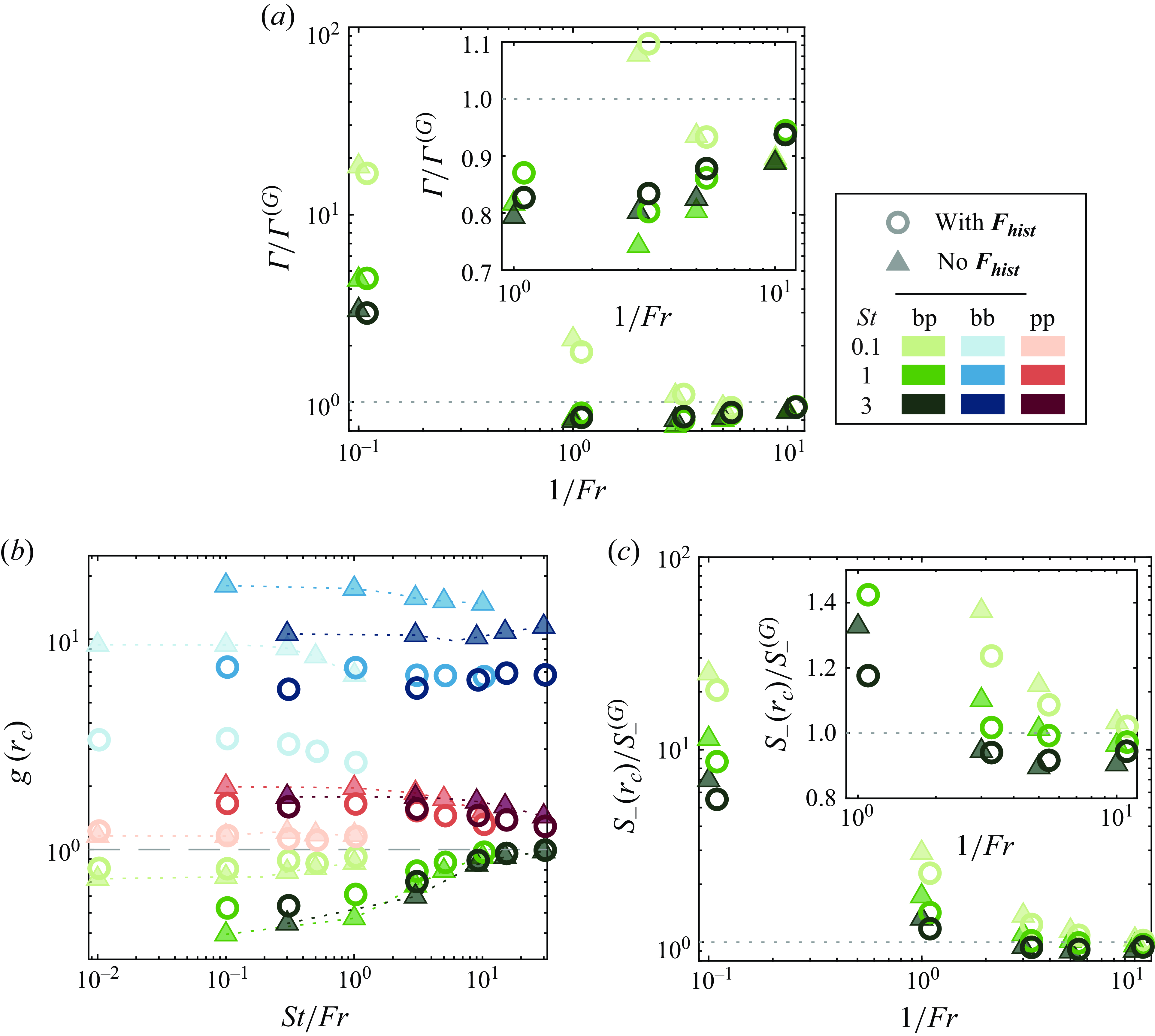
Figure 10. (a) The collision kernel $\Gamma$
normalised by the relative settling limit, (b) the RDF
$\Gamma$
normalised by the relative settling limit, (b) the RDF $g(r_c)$
and (c)
$g(r_c)$
and (c) $S_-(r_c)$
normalised by the relative settling limit for the cases with and without the history force
$S_-(r_c)$
normalised by the relative settling limit for the cases with and without the history force $\boldsymbol{F_{hist}}$
at
$\boldsymbol{F_{hist}}$
at $Re_\lambda = 167$
. The insets in (a) and (c) are zooms in on the
$Re_\lambda = 167$
. The insets in (a) and (c) are zooms in on the $1 \lesssim 1/Fr \lesssim 10$
region.
$1 \lesssim 1/Fr \lesssim 10$
region.
5. Discussion and conclusion
We studied the effect of gravity on bubble–particle collisions in HIT by conducting direct numerical simulations using the point-particle approach (Gatignol Reference Gatignol1983; Maxey & Riley Reference Maxey and Riley1983; Auton Reference Auton1987; Auton et al. Reference Auton, Hunt and Prud’Homme1988). From our simulations, we find that gravity is negligible and turbulence mechanisms determine the collision kernel up to $1/Fr = 0.1$
. For instance, bubbles and particles form individual clusters and segregate in this regime. When
$1/Fr = 0.1$
. For instance, bubbles and particles form individual clusters and segregate in this regime. When $1 \lesssim 1/Fr \lt 10$
, gravity noticeably influences the collision kernel even though the effects of turbulence are still significant. Gravity increases the collision kernel by reducing the extent of segregation and increasing the collision velocity since bubbles rise and particles settle. Notably, the collision kernel dips below the still fluid case when
$1 \lesssim 1/Fr \lt 10$
, gravity noticeably influences the collision kernel even though the effects of turbulence are still significant. Gravity increases the collision kernel by reducing the extent of segregation and increasing the collision velocity since bubbles rise and particles settle. Notably, the collision kernel dips below the still fluid case when $1/Fr \gtrsim 5$
for
$1/Fr \gtrsim 5$
for $St = 0.1$
and
$St = 0.1$
and $1/Fr \gtrsim 1$
for
$1/Fr \gtrsim 1$
for $St \geqslant 0.5$
, meaning turbulence reduces the collision rate in this regime. This is due to preferential sampling and additionally for
$St \geqslant 0.5$
, meaning turbulence reduces the collision rate in this regime. This is due to preferential sampling and additionally for $St \gt 0.5$
a reduction in the bubble slip velocity due to nonlinear drag. Since both effects weaken as
$St \gt 0.5$
a reduction in the bubble slip velocity due to nonlinear drag. Since both effects weaken as $1/Fr$
increases, turbulence effects become negligible and the collision kernel is well approximated by the still fluid case when
$1/Fr$
increases, turbulence effects become negligible and the collision kernel is well approximated by the still fluid case when $1/Fr \geqslant 10$
. For our tested parameters, additional simulations reveal that the observed trends of the bubble–particle collision statistics are not sensitive to particle density and the history force. Quantitatively, the history force tends to reduce bubble–particle segregation and the effective bubble–particle radial approach velocity. These two phenomena have opposite effects on the collision kernel, such that the net effect of the history force on the collision kernel is weak. Although the existing bubble–particle collision models qualitatively capture the increasing trend in the collision velocity with
$1/Fr \geqslant 10$
. For our tested parameters, additional simulations reveal that the observed trends of the bubble–particle collision statistics are not sensitive to particle density and the history force. Quantitatively, the history force tends to reduce bubble–particle segregation and the effective bubble–particle radial approach velocity. These two phenomena have opposite effects on the collision kernel, such that the net effect of the history force on the collision kernel is weak. Although the existing bubble–particle collision models qualitatively capture the increasing trend in the collision velocity with $1/Fr$
over the tested range, none of them achieve quantitative agreement with the simulation data in terms of the collision kernel even when the predictions are appropriately compared with simulations without the history force. We extended the model by Dodin & Elperin (Reference Dodin and Elperin2002) to the bubble–particle case and found excellent agreement with our simulations over all
$1/Fr$
over the tested range, none of them achieve quantitative agreement with the simulation data in terms of the collision kernel even when the predictions are appropriately compared with simulations without the history force. We extended the model by Dodin & Elperin (Reference Dodin and Elperin2002) to the bubble–particle case and found excellent agreement with our simulations over all $1/Fr$
for small
$1/Fr$
for small $St$
if segregation is accounted for and when the history force is neglected. Note that none of these models capture
$St$
if segregation is accounted for and when the history force is neglected. Note that none of these models capture $S_- \lt S_-^{(G)}$
, which occurs at higher
$S_- \lt S_-^{(G)}$
, which occurs at higher $St$
due to the effect of nonlinear drag. This leads to a discrepancy of up to 20 % in
$St$
due to the effect of nonlinear drag. This leads to a discrepancy of up to 20 % in $S_-$
in the tested regime.
$S_-$
in the tested regime.
Throughout this paper, we have used both $1/Fr$
and
$1/Fr$
and $St/Fr$
in order to parameterise the turbulence-to-gravity transition and the gravity-dominated limit. As discussed, gravity starts to play a noticeable role when
$St/Fr$
in order to parameterise the turbulence-to-gravity transition and the gravity-dominated limit. As discussed, gravity starts to play a noticeable role when $1/Fr \gtrsim 1$
. To understand why
$1/Fr \gtrsim 1$
. To understand why $1/Fr$
is the relevant parameter, first take
$1/Fr$
is the relevant parameter, first take $\boldsymbol{\Delta v}$
as a proxy for
$\boldsymbol{\Delta v}$
as a proxy for $S_-$
and consider the following heuristic argument: at small
$S_-$
and consider the following heuristic argument: at small $St$
, the bubble–particle relative velocity
$St$
, the bubble–particle relative velocity $\boldsymbol{\Delta v}$
is given by the shear mechanism which is
$\boldsymbol{\Delta v}$
is given by the shear mechanism which is $\propto \sqrt {St}$
, the local turnstile mechanism which is
$\propto \sqrt {St}$
, the local turnstile mechanism which is $\propto St$
, and the relative settling contribution which is
$\propto St$
, and the relative settling contribution which is $\propto St/Fr$
(see (B2)). Assuming the shear mechanism is weaker than the local turnstile mechanism,
$\propto St/Fr$
(see (B2)). Assuming the shear mechanism is weaker than the local turnstile mechanism, $\boldsymbol{\Delta v} \propto St + St/Fr$
. As
$\boldsymbol{\Delta v} \propto St + St/Fr$
. As $(\boldsymbol{\Delta v})/(\boldsymbol{\Delta v}|_{1/Fr=0}) \propto 1 + 1/Fr$
, we consider
$(\boldsymbol{\Delta v})/(\boldsymbol{\Delta v}|_{1/Fr=0}) \propto 1 + 1/Fr$
, we consider $1/Fr$
when examining the turbulence-to-gravity transition. On the other hand,
$1/Fr$
when examining the turbulence-to-gravity transition. On the other hand, $St/Fr$
is the appropriate non-dimensional number for the gravity-dominant limit as relative settling is governed by
$St/Fr$
is the appropriate non-dimensional number for the gravity-dominant limit as relative settling is governed by $St/Fr$
(Good et al. Reference Good, Ireland, Bewley, Bodenschatz, Collins and Warhaft2014).
$St/Fr$
(Good et al. Reference Good, Ireland, Bewley, Bodenschatz, Collins and Warhaft2014).
Multiple questions still remain to be addressed. Our simulations are conducted using the point-particle approximation, which helps to provide a first-order appreciation of bubble–particle collisions and enables one-to-one comparison with the geometric collision models. As a trade-off for its relative simplicity, this approach limits access to the large- $St$
regime and inherently neglects finite-size effects. For the largest values of
$St$
regime and inherently neglects finite-size effects. For the largest values of $St$
tested
$St$
tested $r_b/\eta \sim 5$
, which is beyond the commonly adopted bounds of the point-particle approximation (Homann & Bec Reference Homann and Bec2010). Therefore, our results at these values should be interpreted with caution as finite-size effects may be relevant. Performing interface-resolved simulation using for example the immersed boundary method (Verzicco Reference Verzicco2023) can provide additional insights as the bubble distorts the local flow field and can further modify the bubble–particle distribution (Tiedemann & Fröhlich Reference Tiedemann and Fröhlich2023; Jiang & Krug Reference Jiang and Krug2025), although the extra complexity would make it harder to distinguish whether the trends in the collision statistics are due to the locally deformed flow field or due to the background turbulence. Furthermore, we considered the more straightforward case of bubbles and particles with the same
$r_b/\eta \sim 5$
, which is beyond the commonly adopted bounds of the point-particle approximation (Homann & Bec Reference Homann and Bec2010). Therefore, our results at these values should be interpreted with caution as finite-size effects may be relevant. Performing interface-resolved simulation using for example the immersed boundary method (Verzicco Reference Verzicco2023) can provide additional insights as the bubble distorts the local flow field and can further modify the bubble–particle distribution (Tiedemann & Fröhlich Reference Tiedemann and Fröhlich2023; Jiang & Krug Reference Jiang and Krug2025), although the extra complexity would make it harder to distinguish whether the trends in the collision statistics are due to the locally deformed flow field or due to the background turbulence. Furthermore, we considered the more straightforward case of bubbles and particles with the same $St$
. While this has provided much understanding into the collision process, unravelling the collision mechanisms for bubbles and particles with different
$St$
. While this has provided much understanding into the collision process, unravelling the collision mechanisms for bubbles and particles with different $St$
would prove invaluable for real life applications, where particles in flotation cells are usually far from monodispersed. In terms of modelling, a theoretical model of segregation will greatly enhance the predictive capabilities of the existing models.
$St$
would prove invaluable for real life applications, where particles in flotation cells are usually far from monodispersed. In terms of modelling, a theoretical model of segregation will greatly enhance the predictive capabilities of the existing models.
Acknowledgements.
We thank G. Piumini, D. van Buuren, K. Zhong and G. Vacca for helpful discussions.
Funding.
This project has received funding from the European Research Council (ERC) under the European Union’s Horizon 2020 research and innovation programme (grant agreement No. 950111, BU-PACT). This work was carried out on the Dutch national e-infrastructure with the support of SURF Cooperative. We acknowledge the EuroHPC Joint Undertaking for awarding the project EHPC-REG-2023R03-178 access to the EuroHPC supercomputer Discoverer, hosted by Sofia Tech Park (Bulgaria).
Declaration of interests.
The authors report no conflict of interest.
Data availability statement.
All data supporting this study are openly available from the 4TU.ResearchData repository at https://doi.org/10.4121/aac3a58a-67ea-4221-8ac0-48a66a5e960c.
Appendix A. Consistent inclusion of gravity following Abrahamson (Reference Abrahamson1975)
The original expression of the collision kernel including gravity as given in Abrahamson (Reference Abrahamson1975) has an integration error which has been partly resolved by Kostoglou et al. (Reference Kostoglou, Karapantsios and Evgenidis2020a ) using a comparable expression. However, the equivalence between the expressions in Abrahamson (Reference Abrahamson1975) and Kostoglou et al. (Reference Kostoglou, Karapantsios and Evgenidis2020a ) was not directly shown. We provide this additional detail in this appendix. Furthermore, we show the difference between (2.7) and the best-fit expressions reported in figure 2 and (10) in Kostoglou et al. (Reference Kostoglou, Karapantsios and Evgenidis2020a ).
According to Abrahamson (Reference Abrahamson1975), the collision kernel between two types of particles in the presence of gravity is given by
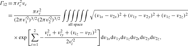 \begin{align} \Gamma _{12} &= \pi r_c^2 v_c\nonumber \\ &= \frac {\pi r_c^2}{(2\pi v_1^{\prime 2})^{3/2}(2\pi v_2^{\prime 2})^{3/2}}\mathop{\int \!\!\int \!\!\int \!\!\int \!\!\int \!\!\int }\limits_{\textrm {all space}} \sqrt {(v_{1x}-v_{2x})^2 + (v_{1y}-v_{2y})^2 + (v_{1z}-v_{2z})^2}\nonumber \\ &\quad \times \exp {\left [\sum _{i = 1}^{2}-\frac {v_{ix}^2 + v_{iy}^2 + (v_{iz} - v_{Ti})^2}{2v_i^{\prime 2}} \right ]} \mathrm{d}v_{1x}\mathrm{d}v_{1y}\mathrm{d}v_{1z}\mathrm{d}v_{2x}\mathrm{d}v_{2y}\mathrm{d}v_{2z}, \end{align}
where the numerical subscripts $1,2$
denote the colliding particles, and the alphabetical subscripts
$1,2$
denote the colliding particles, and the alphabetical subscripts $x,y,z$
denote the corresponding velocity components. Changing variables such that
$x,y,z$
denote the corresponding velocity components. Changing variables such that $v_{iN} = v_{iz} - v_{Ti}$
for
$v_{iN} = v_{iz} - v_{Ti}$
for $i = 1,2$
and further taking
$i = 1,2$
and further taking
 \begin{align} v_{xm} &= \frac {v_{1x} + v_{2x}}{2}, \quad v_{ym} = \frac {v_{1y} + v_{2y}}{2}, \quad v_{zm} = \frac {v_{1N} + v_{2N}}{2} ,\end{align}
 \begin{align} v_{xd} &= v_{1x} - v_{2x}, \quad v_{yd} = v_{1y} - v_{2y}, \quad v_{zd} = v_{1N} - v_{2N} ,\end{align}
yields
 \begin{align} v_c &= \frac {1}{(2\pi v_1^{\prime 2})^{3/2}(2\pi v_2^{\prime 2})^{3/2}}\iiint \limits _{\mathrm{all\,space}} \sqrt {v_{xd}^2 + v_{yd}^2 + [v_{zd} + (v_{T1} - v_{T2})]^2}\nonumber \\ &\quad \times I_x \cdot I_y \cdot I_z\cdot \mathrm{d}v_{xd}\mathrm{d}v_{yd}\mathrm{d}v_{zd}, \end{align}
where
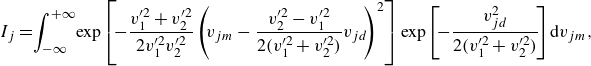 \begin{equation} I_j = \!\int _{-\infty }^{+\infty }\! \exp \left [\!-\frac {v_1^{\prime 2} + v_2^{\prime 2}}{2v_1^{\prime 2}v_2^{\prime 2}}\left ( \! v_{jm} - \frac {v_2^{\prime 2} - v_1^{\prime 2}}{2(v_1^{\prime 2} + v_2^{\prime 2})} v_{jd}\!\right )^2 \right ] \exp \left [\!-\frac {v_{jd}^2}{2(v_1^{\prime 2} + v_2^{\prime 2})} \!\right ] \mathrm{d}v_{jm} ,\end{equation}
and $j = x,y,z$
. Using
$j = x,y,z$
. Using $\int _{-\infty }^{+\infty }\exp [-a(x-b)^2]\mathrm{d}x = \sqrt {\pi /a}$
where
$\int _{-\infty }^{+\infty }\exp [-a(x-b)^2]\mathrm{d}x = \sqrt {\pi /a}$
where $a,b$
are constants to evaluate
$a,b$
are constants to evaluate $I_x$
,
$I_x$
, $I_y$
and
$I_y$
and $I_z$
$I_z$
 \begin{align} v_c &= \frac {1}{[2\pi (v_1^{\prime 2} + v_2^{\prime 2})]^{3/2}}\iiint \limits _{\mathrm{all\,space}} \sqrt {v_{xd}^2 + v_{yd}^2 + [v_{zd} + (v_{T1} - v_{T2})]^2}\nonumber \\ &\quad \times \exp \left [ -\frac {v_{xd}^2 + v_{yd}^2 + v_{zd}^2}{2(v_1^{\prime 2} + v_2^{\prime 2})} \right ] \mathrm{d}v_{xd}\mathrm{d}v_{yd}\mathrm{d}v_{zd}, \end{align}
which is the same as (8) in Kostoglou et al. (Reference Kostoglou, Karapantsios and Evgenidis2020a ) with the following mapping:
 \begin{align} \sqrt {v_1^{\prime 2} + v_2^{\prime 2}} \to V, \!\!\!\!\quad v_{T2} - v_{T1} \to U_B, \!\!\!\!\quad v_c \to U_T, \!\!\!\!\quad \frac {v_{T2} - v_{T1}}{\sqrt{v_1^{\prime 2} + v_2^{\prime 2}}} \to \alpha , \!\!\!\!\quad \frac {v_c}{\sqrt {v_1^{\prime 2} + v_2^{\prime 2}}} \to \Psi . \end{align}
Kostoglou et al. (Reference Kostoglou, Karapantsios and Evgenidis2020a ) numerically integrated (A5), showed a best-fit result in their figure 2 and stated in their (10) that the corresponding equation is
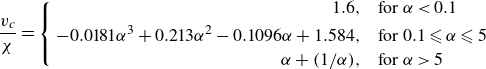 \begin{equation} \frac {v_c}{\chi } = \left \{ \begin{aligned} 1.6, \quad &\text{for $\alpha \lt 0.1$}\\ -0.0181\alpha ^3+0.213\alpha ^2-0.1096\alpha +1.584,\quad &\text{for $0.1\leqslant \alpha \leqslant 5$}\\ \alpha + (1/\alpha ),\quad &\text{for $\alpha \gt 5$} \end{aligned} \right . \end{equation}
where $\alpha = (v_{T2}-v_{T1})/\chi$
and
$\alpha = (v_{T2}-v_{T1})/\chi$
and $\chi = \sqrt {v^{\prime 2}_1 + v^{\prime 2}_2}$
. Both the curve shown in their figure 2 and (A7) are plotted in figure 11, which clearly indicates their difference. We additionally include our best-fit expression (2.7), which shows excellent agreement with the numerical integration result as displayed in figure 2 of Kostoglou et al. (Reference Kostoglou, Karapantsios and Evgenidis2020a
).
$\chi = \sqrt {v^{\prime 2}_1 + v^{\prime 2}_2}$
. Both the curve shown in their figure 2 and (A7) are plotted in figure 11, which clearly indicates their difference. We additionally include our best-fit expression (2.7), which shows excellent agreement with the numerical integration result as displayed in figure 2 of Kostoglou et al. (Reference Kostoglou, Karapantsios and Evgenidis2020a
).


Appendix B. Extension of the Dodin & Elperin (Reference Dodin and Elperin2002) model to particles with different densities
The Dodin & Elperin (Reference Dodin and Elperin2002) model is applicable for infinitely heavy inertial particles with a uniform spatial distribution in HIT. Here, we extend it to particles with different densities by incorporating the density ratio $\beta _i = 2(\rho _f - \rho _i)/(\rho _f + 2\rho _i)$
.
$\beta _i = 2(\rho _f - \rho _i)/(\rho _f + 2\rho _i)$
.
We start from (3.2) in the small $St$
limit without lift (Fouxon Reference Fouxon2012)
$St$
limit without lift (Fouxon Reference Fouxon2012)
 \begin{equation} \boldsymbol{v_i} = \boldsymbol{u} + \frac {\beta _i\tau _i}{f_i}\boldsymbol{\psi } + \frac {\beta _i\tau _i}{f_i}\mathfrak{g}\boldsymbol{e_z}, \end{equation}
where $\boldsymbol{\psi } = D\boldsymbol{u}/Dt$
. Consider the case where two particles located at positions
$\boldsymbol{\psi } = D\boldsymbol{u}/Dt$
. Consider the case where two particles located at positions $A$
and
$A$
and $B$
are at collision distance such that their separation is small. Here,
$B$
are at collision distance such that their separation is small. Here, $\boldsymbol{\psi }|_A\approx \boldsymbol{\psi }|_B$
and
$\boldsymbol{\psi }|_A\approx \boldsymbol{\psi }|_B$
and
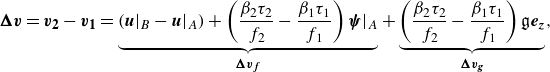 \begin{equation} \boldsymbol{\Delta v} = \boldsymbol{v_2} - \boldsymbol{v_1} = \underbrace {(\boldsymbol{u}|_B - \boldsymbol{u}|_A) + \left (\frac {\beta _2\tau _2}{f_2} - \frac {\beta _1\tau _1}{f_1}\right )\boldsymbol{\psi }|_A}_{\boldsymbol{\Delta v_f}} + \underbrace {\left (\frac {\beta _2\tau _2}{f_2} - \frac {\beta _1\tau _1}{f_1}\right )\mathfrak{g}\boldsymbol{e_z}}_{\boldsymbol{\Delta v_g}}, \end{equation}
in which $\boldsymbol{\Delta v}$
has been split into fluid
$\boldsymbol{\Delta v}$
has been split into fluid $\boldsymbol{\Delta v_f}$
and gravity contributions
$\boldsymbol{\Delta v_f}$
and gravity contributions $\boldsymbol{\Delta v_g}$
. Projecting (B2) along the separation vector, of which
$\boldsymbol{\Delta v_g}$
. Projecting (B2) along the separation vector, of which $\boldsymbol{e_r}$
is the corresponding unit vector, gives
$\boldsymbol{e_r}$
is the corresponding unit vector, gives
 \begin{equation} \Delta v_r(\theta ) = (\boldsymbol{\Delta v_f} + \boldsymbol{\Delta v_g})\cdot \boldsymbol{e_r} := \xi + h(\theta ) = \xi + \left (\frac {\beta _2\tau _2}{f_2} - \frac {\beta _1\tau _1}{f_1}\right )\mathfrak{g}\cos \theta . \end{equation}
As the background flow is HIT, $\xi$
is isotropic so it is assumed to be normally distributed. Furthermore, since
$\xi$
is isotropic so it is assumed to be normally distributed. Furthermore, since $h(\theta )$
has a sign ambiguity originating from the possibility of labelling either particle as number 1, we introduce
$h(\theta )$
has a sign ambiguity originating from the possibility of labelling either particle as number 1, we introduce
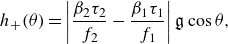 \begin{equation} h_+(\theta ) = \left |\frac {\beta _2\tau _2}{f_2} - \frac {\beta _1\tau _1}{f_1}\right |\mathfrak{g}\cos \theta ,\end{equation}
and write
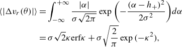 \begin{align} \langle |\Delta v_r(\theta )|\rangle &= \int _{-\infty }^{+\infty } \frac {|\alpha |}{\sigma \sqrt {2\pi }}\exp {\left (-\frac {(\alpha - h_+)^2}{2\sigma ^2}\right )}d\alpha \nonumber \\ &= \sigma \sqrt {2}\kappa \textrm {erf}\kappa + \sigma \sqrt {\frac {2}{\pi }}\exp {(-\kappa ^2)}, \end{align}
where $\langle \cdot \rangle$
denotes averaging,
$\langle \cdot \rangle$
denotes averaging, $\kappa = h_+/(\sigma \sqrt {2})$
and
$\kappa = h_+/(\sigma \sqrt {2})$
and $\sigma = \sqrt {\langle \xi ^2\rangle } =\sigma _{\Delta vr}^{(DEX)}$
is the r.m.s. of
$\sigma = \sqrt {\langle \xi ^2\rangle } =\sigma _{\Delta vr}^{(DEX)}$
is the r.m.s. of $\xi$
(we drop the subscript and superscript of
$\xi$
(we drop the subscript and superscript of $\sigma _{\Delta vr}^{(DEX)}$
in this appendix to reduce clutter). For
$\sigma _{\Delta vr}^{(DEX)}$
in this appendix to reduce clutter). For $\sigma$
, we use the isotropy of the background flow and place particle 2 along the
$\sigma$
, we use the isotropy of the background flow and place particle 2 along the $x$
-axis at position C. Similar to before, we consider particles at collision distance so
$x$
-axis at position C. Similar to before, we consider particles at collision distance so $\boldsymbol{\psi }|_A \approx \boldsymbol{\psi }|_C$
, meaning
$\boldsymbol{\psi }|_A \approx \boldsymbol{\psi }|_C$
, meaning
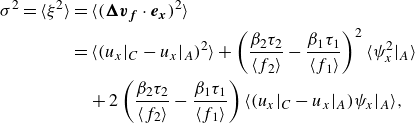 \begin{align} \sigma ^2 = \langle \xi ^2\rangle &= \langle (\boldsymbol{\Delta v_f}\cdot \boldsymbol{e_x})^2\rangle \nonumber \\ &= \langle (u_x|_C - u_x|_A)^2 \rangle + \left (\frac {\beta _2\tau _2}{\langle f_2 \rangle } - \frac {\beta _1\tau _1}{\langle f_1 \rangle }\right )^2\langle \psi _x^2|_A \rangle \nonumber \\ &\quad + 2\left (\frac {\beta _2\tau _2}{\langle f_2 \rangle } - \frac {\beta _1\tau _1}{\langle f_1 \rangle }\right )\langle (u_x|_C - u_x|_A)\psi _x|_A \rangle , \end{align}
where $\psi _x = Du_x/Dt$
. Additionally, as
$\psi _x = Du_x/Dt$
. Additionally, as $\langle (u_x|_C - u_x|_A)\psi _x|_A\rangle \approx \langle {(u_x|_C - u_x|_A)\psi _x|_C}\rangle = - \langle {(u_x|_C - u_x|_A)\psi _x|_A}\rangle$
due to homogeneity,
$\langle (u_x|_C - u_x|_A)\psi _x|_A\rangle \approx \langle {(u_x|_C - u_x|_A)\psi _x|_C}\rangle = - \langle {(u_x|_C - u_x|_A)\psi _x|_A}\rangle$
due to homogeneity, $\langle {(u_x|_C - u_x|_A)\psi _x|_A} \rangle \approx 0$
. Therefore,
$\langle {(u_x|_C - u_x|_A)\psi _x|_A} \rangle \approx 0$
. Therefore,
 \begin{equation} \sigma ^2 = r_c^2\left \langle {\left (\frac {\partial u_x}{\partial x}\right )^2}\right \rangle + \left (\frac {\beta _2\tau _2}{\langle f_2\rangle } - \frac {\beta _1\tau _1}{\langle f_1\rangle }\right )^2 \left \langle {\left (\frac {Du_x}{Dt}\right )^2}\right \rangle := r_c^2\gamma ^2 + \left (\frac {\beta _2\tau _2}{\langle f_2\rangle } - \frac {\beta _1\tau _1}{\langle f_1\rangle }\right )^2\lambda ^2, \end{equation}
where $\gamma ^2 = \langle (\partial u_x/\partial x)^2\rangle = \varepsilon /(15\nu )$
and
$\gamma ^2 = \langle (\partial u_x/\partial x)^2\rangle = \varepsilon /(15\nu )$
and $\lambda ^2 = \langle (Du_x/Dt)^2\rangle = 1.3\varepsilon ^{3/2}\nu ^{-1/2}$
.
$\lambda ^2 = \langle (Du_x/Dt)^2\rangle = 1.3\varepsilon ^{3/2}\nu ^{-1/2}$
.
Finally, note that, in the case where $g(r_c)=1$
,
$g(r_c)=1$
,
 \begin{equation} \Gamma _{12} = \tfrac {1}{2} \int _{0}^{\pi } \langle {|\Delta v_r(\theta )|}\rangle (2\pi r_c \sin \theta ) r_c d\theta = \pi r_c^2 \int _{0}^{\pi } \langle {|\Delta v_r(\theta )|}\rangle \sin \theta d\theta , \end{equation}
where the factor $1/2$
in the first equality singles out the inward flux of particles across the collision sphere assuming flux balance. This equation can be further simplified using symmetry of
$1/2$
in the first equality singles out the inward flux of particles across the collision sphere assuming flux balance. This equation can be further simplified using symmetry of $\langle |\Delta v_r(\theta )|\rangle$
 \begin{equation} \langle |\Delta v_r(\pi - \theta )|\rangle = \langle |\xi - h(\theta )|\rangle = \langle |-\xi + h(\theta )|\rangle = \langle |\Delta v_r(\theta )|\rangle , \end{equation}
where the final equality is attributed to the symmetry of the distribution of $\xi$
about 0. Equation (B8) then becomes
$\xi$
about 0. Equation (B8) then becomes
 \begin{equation} \Gamma _{12} = 2\pi r_c^2 \int _{0}^{\pi /2} \langle {|\Delta v_r(\theta )|}\rangle \sin \theta {\rm d}\theta . \end{equation}
Performing the integration results in
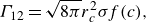 \begin{equation} \Gamma _{12} = \sqrt {8\pi }r_c^2\sigma f(c), \end{equation}
where
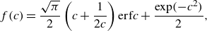 \begin{equation} f(c) = \frac {\sqrt {\pi }}{2}\left (c + \frac {1}{2c}\right )\textrm {erf} c + \frac {\exp (-c^2)}{2} ,\end{equation}
and
 \begin{equation} c = \frac {|\beta _2\tau _2/\langle f_2\rangle - \beta _1\tau _1/\langle f_1\rangle |\mathfrak{g}}{\sqrt {2}\sigma }. \end{equation}
Appendix C. Domain size effects
The simulations reported are conducted in a cubic domain with $L_{box} = 1$
. With gravity, bubble and particle statistics may exhibit periodicity effects if the time taken by the bubbles and particles to travel through the periodic simulation domain is less than the eddy turnover time, i.e.
$L_{box} = 1$
. With gravity, bubble and particle statistics may exhibit periodicity effects if the time taken by the bubbles and particles to travel through the periodic simulation domain is less than the eddy turnover time, i.e. $T_{box,i} \lt \ell /u'$
(Woittiez et al. Reference Woittiez, Jonker and Portela2009), where
$T_{box,i} \lt \ell /u'$
(Woittiez et al. Reference Woittiez, Jonker and Portela2009), where $\ell$
is the integral length scale. Taking
$\ell$
is the integral length scale. Taking $T_{box,i} \sim L_{boxz}/|\beta _i|\tau _i\mathfrak{g}$
, this means
$T_{box,i} \sim L_{boxz}/|\beta _i|\tau _i\mathfrak{g}$
, this means
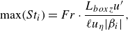 \begin{equation} \max (St_i) = Fr\cdot \frac {L_{boxz}u'}{\ell u_\eta |\beta _i|}, \end{equation}
where $L_{boxz}$
is the vertical domain size. Table 2 shows that the maximum
$L_{boxz}$
is the vertical domain size. Table 2 shows that the maximum $St$
is not exceeded with
$St$
is not exceeded with $L_{boxz} = 1$
even for the largest
$L_{boxz} = 1$
even for the largest $St_b$
and
$St_b$
and $St_p$
simulated except for the
$St_p$
simulated except for the $(Re_\lambda ,1/Fr) = (69,10)$
case. To confirm the collision statistics are not affected even then, we lengthen the simulation domain along the vertical direction following Chouippe & Uhlmann (Reference Chouippe and Uhlmann2015) and rerun the
$(Re_\lambda ,1/Fr) = (69,10)$
case. To confirm the collision statistics are not affected even then, we lengthen the simulation domain along the vertical direction following Chouippe & Uhlmann (Reference Chouippe and Uhlmann2015) and rerun the $(St,1/Fr) = (3,10)$
cases. Figure 12 shows that
$(St,1/Fr) = (3,10)$
cases. Figure 12 shows that $\Gamma (r)$
,
$\Gamma (r)$
, $g(r)$
and
$g(r)$
and $S_-(r)$
are not sensitive to
$S_-(r)$
are not sensitive to $L_{boxz}$
for bubble–particle, bubble–bubble and particle–particle collisions.
$L_{boxz}$
for bubble–particle, bubble–bubble and particle–particle collisions.
Table 2. The maximum $St$
that satisfies the criterion in (C1) when
$St$
that satisfies the criterion in (C1) when $L_{boxz} = 1$
.
$L_{boxz} = 1$
.
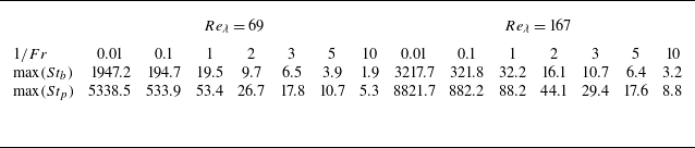
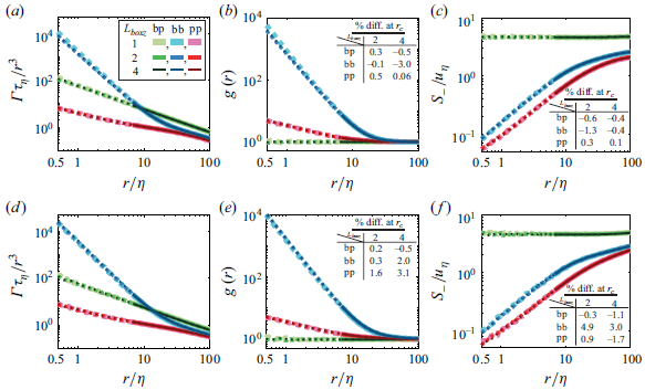
Figure 12. The (a) collision kernel, (b) RDF and (c) effective radial approach velocity with different $L_{boxz}$
at
$L_{boxz}$
at $Re_\lambda = 69$
and (d–f)
$Re_\lambda = 69$
and (d–f) $Re_\lambda = 167$
. The dotted segments indicate
$Re_\lambda = 167$
. The dotted segments indicate $r \lt r_c$
. The tables in (b–c) and (e–f) show the percentage difference of the values at
$r \lt r_c$
. The tables in (b–c) and (e–f) show the percentage difference of the values at $r_c$
compared with the
$r_c$
compared with the $L_{boxz} = 1$
case.
$L_{boxz} = 1$
case.
Appendix D. Code verification
The code used in this study is identical to the already verified code used in Chan et al. (Reference Chan, Ng and Krug2023) apart from the addition of the buoyancy, history force and lift terms. To verify the buoyancy term, we first omit the history force and simulate 100 bubbles rising in still fluid. Figure 13(a) shows that their terminal rise velocities correspond to the theoretical value ( $v_T=0.117$
). We next add the history force and consider a particle settling in still fluid. Here, we employ Stokes drag (
$v_T=0.117$
). We next add the history force and consider a particle settling in still fluid. Here, we employ Stokes drag ( $f_p = 1$
) to enable comparison with the analytical solution of the velocity time series by van Hinsberg et al. (Reference van Hinsberg, ten Thije Boonkkamp and Clercx2011). As shown in figure 13(a), the numerical and analytic solutions agree perfectly when the window length of the history force spans the entire simulation duration, and the agreement is still excellent if a window length of
$f_p = 1$
) to enable comparison with the analytical solution of the velocity time series by van Hinsberg et al. (Reference van Hinsberg, ten Thije Boonkkamp and Clercx2011). As shown in figure 13(a), the numerical and analytic solutions agree perfectly when the window length of the history force spans the entire simulation duration, and the agreement is still excellent if a window length of $t_w/(\nu /\mathfrak{g}^2)^{1/3} = 0.07$
, which corresponds to 5 time steps, is used.
$t_w/(\nu /\mathfrak{g}^2)^{1/3} = 0.07$
, which corresponds to 5 time steps, is used.
For the lift term, we checked that the lift force acting on a bubble in a simple shear flow with $\partial u_z/\partial x = 0.64$
is equal to the manually computed value given by the lift force expression in figure 13(b).
$\partial u_z/\partial x = 0.64$
is equal to the manually computed value given by the lift force expression in figure 13(b).
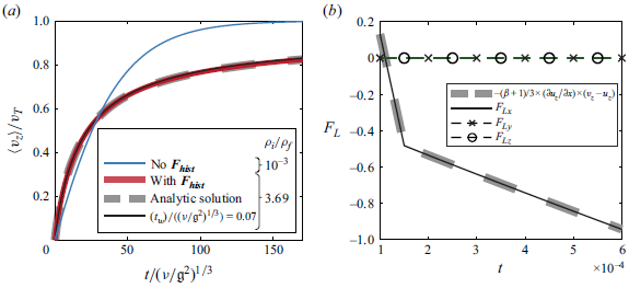
Figure 13. (a) Time series of the mean vertical velocity of 100 bubbles rising in quiescent liquid (blue line) with a Galileo number $Ga_b = \sqrt {\mathfrak{g}(2r_b)^3|\rho _b/\rho _f - 1|}/\nu = 106$
,
$Ga_b = \sqrt {\mathfrak{g}(2r_b)^3|\rho _b/\rho _f - 1|}/\nu = 106$
, $\rho _b/\rho _f = 1/1000$
and nonlinear drag
$\rho _b/\rho _f = 1/1000$
and nonlinear drag $f_b = 1 + 0.169Re_b^{2/3}$
, as well as that of a particle settling in quiescent liquid with
$f_b = 1 + 0.169Re_b^{2/3}$
, as well as that of a particle settling in quiescent liquid with $Ga_p = 36$
,
$Ga_p = 36$
, $\rho _p/\rho _f = 3.69$
and Stokes drag
$\rho _p/\rho _f = 3.69$
and Stokes drag $f_p = 1$
. (b) The lift force acting on a bubble with
$f_p = 1$
. (b) The lift force acting on a bubble with $(Ga_b,\rho _b/\rho _f) = (106, 1/1000)$
and nonlinear drag
$(Ga_b,\rho _b/\rho _f) = (106, 1/1000)$
and nonlinear drag $f_b = 1 + 0.169Re_b^{2/3}$
in a simple shear flow.
$f_b = 1 + 0.169Re_b^{2/3}$
in a simple shear flow.


 Open access