


1. Introduction
Turbulence is ever present in nature and in numerous man-made processes. Wall-bounded turbulent flows, in particular, are extremely important for technological applications. Close to 25 % of the energy used in industry is destined to transport fluids in pipes and channels, or to propel vehicles through air or water, and approximately a quarter of that energy is irreversibly dissipated by turbulence in regions close to walls (Jiménez Reference Jiménez2013). Moreover, in several industrial settings, the transported fluid is non-Newtonian. A non-Newtonian fluid exhibits non-constant viscosity which may depend on shear stress and/or strain rate history in a nonlinear manner and can be classified within three main groups (Irgens Reference Irgens2014): (i) time-independent fluids, which are further divided into viscoplastic/yield-stress fluids and purely viscous fluids, (ii) time-dependent fluids and (iii) viscoelastic fluids consisting of materials with both elastic and viscous effects.
Considering the previous context, this work focuses on purely viscous fluids and is an extension of the turbulent channel flow study of Arosemena, Andersson & Solsvik (Reference Arosemena, Andersson and Solsvik2021). Our aim is to explore the changes on the near-wall turbulent structures, in particular the quasi-streamwise vortices, due to shear-thinning fluid behaviour; a non-Newtonian rheology exhibiting drag-reducing features.
1.1. Rheological drag reduction in generalized Newtonian fluids
Although elastic effects are present in several drag-reducing fluids, within a given range of particle concentration and for certain polymer solutions such effects are negligible; e.g. consider the variations of the elastic recovery index (Durán et al. Reference Durán, Ramos-Tejada, Arroyo and González-Caballero2000) in solutions with a concentration of less than 2.5 wt% of carboxymethyl cellulose reported by Benchabane & Bekkour (Reference Benchabane and Bekkour2008). Generalized Newtonian (GN) fluids are a type of time-independent, purely viscous fluids which stress tensor due to viscous effects,  ${\tau _{ij}}_{vis}$, is given by
 \begin{equation} {\tau_{ij}}_{vis} =2 \mu {\mathsf{S}}_{ij}, \end{equation}
where  $\mu = \mu (\dot {\gamma })$ is the apparent dynamic viscosity solely depending on the strain rate $\dot {\gamma }=(2{\mathsf{S}}_{ij}{\mathsf{S}}_{ji})^{1/2}$ and ${\mathsf{S}}_{ij}$ is the strain rate tensor. GN fluids are commonly encountered in various industrial and commercial applications and those of non-Newtonian nature are classified into pseudoplastic/shear-thinning and dilatant/shear-thickening fluids based on the observed trend in their apparent viscosity with increasing strain rate. Regarding the shear-thinning fluids, they exhibit decreasing apparent viscosity with increasing strain rate and are frequently found in bioreactors, in drilling activities within the petroleum industry and are used as additives in cosmetic and food products. Polymer solutions with shear-thinning behaviour such as those with concentrations of carboxymethyl cellulose, xanthan gum and polyacrylamide, are also commonly used for turbulent flow experiments of drag-reducing non-Newtonian fluids (Escudier et al. Reference Escudier, Gouldson, Pereira, Pinho and Poole2001).
Many experimental (Park et al. Reference Park, Mannheimer, Grimley and Morrow1989; Pinho & Whitelaw Reference Pinho and Whitelaw1990; Pereira Reference Pereira and Pinho1994) and numerical (Rudman & Blackburn Reference Rudman and Blackburn2003, Reference Rudman and Blackburn2006; Gavrilov & Rudyak Reference Gavrilov and Rudyak2016) studies have reported features common to the low drag reduction (LDR) regime (Warholic, Massah & Hanratty Reference Warholic, Massah and Hanratty1999), such as enhancement of streamwise turbulence intensity and suppression of other cross-sectional intensities, decrease in Reynolds shear stress and overall reduction of turbulent production with shear-thinning fluid behaviour. More recently, and based on observations of the Reynolds stress budgets and to the overall turbulent kinetic energy, for turbulent pipe (Singh, Rudman & Blackburn Reference Singh, Rudman and Blackburn2017) and channel (Arosemena et al. Reference Arosemena, Andersson and Solsvik2021) flows, strain-rate-dependent rheology has been found to be mainly important within the inner layer region. This remark is supported as well by the Singh, Rudman & Blackburn (Reference Singh, Rudman and Blackburn2016) results where, for a fixed GN fluid rheology within the inner layer region, no significant differences are observed in the mean-flow and first-order statistics even if different apparent fluid viscosity profiles are attained outside the inner layer. Singh, Rudman & Blackburn (Reference Singh, Rudman and Blackburn2018) also reported small contributions from viscosity fluctuation terms to the mean shear stress budget, mean flow and turbulent kinetic energy budget up to moderate frictional Reynolds numbers,  $Re_{\tau }=323\text {--}750$. Arosemena et al. (Reference Arosemena, Andersson and Solsvik2021) further reasoned that observed drag-reducing features with shear-thinning behaviour are likely related to important changes to the near-wall turbulent structures and, in consequence, to the self-sustaining process occurring near the wall.
1.2. Near-wall self-sustaining process
The inner region of wall-bounded turbulent shear flows has been extensively investigated and remarkable well-organized coherent structures have been found. In the vicinity to the wall, where shear dominates, flow visualizations by Kline et al. (Reference Kline, Reynolds, Schraub and Runstadler1967) in boundary layers and by Corino & Brodkey (Reference Corino and Brodkey1969) in pipes revealed regions of low- and high-speed fluid (‘streaks’) staggered in the spanwise direction. Such streaks undergo a series of dynamical processes leading to production of turbulence; during an intermittent, quasi-cyclical process, outward ejections of low-speed fluid and inrush of high-speed fluid towards the wall occur (Wallace, Eckelmann & Brodkey Reference Wallace, Eckelmann and Brodkey1972; Willmarth & Lu Reference Willmarth and Lu1972). The other important near-wall structures consist of quasi-streamwise vortices or rolls. The streaks contain most of the turbulent kinetic energy and the vortices both organize the energy dissipation and the momentum transfer (Jiménez Reference Jiménez2013).
A recurring topic in the study of near-wall structures is the regeneration cycle involving the streaks and vortices. While it is generally accepted that the quasi-streamwise vortices cause the streaks by advection of the mean velocity gradient (Blackwelder & Eckelmann Reference Blackwelder and Eckelmann1979) and with independence from the presence of the wall (Lee, Kim & Moin Reference Lee, Kim and Moin1990), there is still uncertainty regarding what causes the rolls. Explanations for the regeneration cycle of near-wall vortical structures can be grouped within two main categories (Schoppa & Hussain Reference Schoppa and Hussain2002): (i) parent–offspring regeneration (see for instance Brooke & Hanratty (Reference Brooke and Hanratty1993) in the case of roll-up of near-wall streamwise vorticity sheets and Zhou et al. (Reference Zhou, Adrian, Balachandar and Kendall1999) for quasi-streamwise vortex generation from hairpin-shaped vortical structures) and (ii) instability-based generation (see for instance Swearingen & Blackwelder Reference Swearingen and Blackwelder1987; Robinson Reference Robinson1991; Jiménez Reference Jiménez1994 or Hamilton, Kim & Waleffe Reference Hamilton, Kim and Waleffe1995 for velocity streak instability-based generation). Jiménez & Pinelli (Reference Jiménez and Pinelli1999) showed that disturbing the streaks in a region where the wall-normal coordinate – in inner viscous/wall units – is less than  $60$ but greater than $20$ inhibits the formation of streamwise vortices and suggested that a regeneration cycle based on streaks instabilities dominates over other mechanisms for the generation of rolls. Jiménez & Pinelli (Reference Jiménez and Pinelli1999) additionally showed that near-wall turbulence is autonomous in the sense that streaks and vortices do not decay even after the outer flow is artificially removed. On the other hand, Schoppa & Hussain (Reference Schoppa and Hussain2002) argued that most buffer streaks are too weak to be unstable to the inflectional mechanism described by Jiménez & Pinelli (Reference Jiménez and Pinelli1999) and proposed an alternative explanation for the streaks instability based on (linear) transient growth of secondary perturbations. Hence, it seems there is no unanimous agreement in how the near-wall vortical structures are produced, albeit the idea of the regeneration of rolls due to the instability of the streaks, leading to their breakdown, is consistent between multiple authors (see also Hoepffner, Brandt & Henningson (Reference Hoepffner, Brandt and Henningson2005) and more recently, Cossu et al. (Reference Cossu, Brandt, Bagheri and Henningson2011)).
Despite the shortcomings in our understanding regarding the near-wall vortex dynamics, we do know that any drag-reducing strategy is based on disturbing the turbulence regeneration cycle (Karniadakis & Choi Reference Karniadakis and Choi2003). Drag reduction can be achieved by decreasing the intensity of the quasi-streamwise vortices or by weakening their interaction with the near-wall flow (Tardu Reference Tardu1995) and the use of riblets (Choi, Moin & Kim Reference Choi, Moin and Kim1993; García-Mayoral & Jiménez Reference García-Mayoral and Jiménez2011) and polymer additives (several studies, e.g. Ptasinski et al. Reference Ptasinski, Boersma, Nieuwstadt, Hulsen, Van Der Brule and Hunt2003; Dubief et al. Reference Dubief, White, Terrapon, Shaqfeh, Moin and Lele2004; Kim et al. Reference Kim, Li, Sureshkumar, Balachandar and Adrian2007; Li & Graham Reference Li and Graham2007; Kim & Sureshkumar Reference Kim and Sureshkumar2013) are within the few successful strategies that actually disrupt the self-sustained regeneration cycle. In polymer solutions, known effects of viscoelasticity on the wall turbulence are the reduction in the strength and numbers of the quasi-streamwise vortices and a reduction in the spanwise meandering and thickening of the streaks (Kim et al. Reference Kim, Li, Sureshkumar, Balachandar and Adrian2007; White & Mungal Reference White and Mungal2008). The self-sustained cycle is seemly disrupted by the polymers which oppose the motion of the vortices (Dubief et al. Reference Dubief, Terrapon, White, Shaqfeh, Moin and Lele2005; Kim et al. Reference Kim, Li, Sureshkumar, Balachandar and Adrian2007), take energy from them and release it into the streaks (Dubief et al. Reference Dubief, White, Terrapon, Shaqfeh, Moin and Lele2004, Reference Dubief, Terrapon, White, Shaqfeh, Moin and Lele2005). In contrast to studies about polymer solutions accounting for viscoelastic effects, works related to drag-reducing GN fluids have not directly addressed probable mechanisms leading to disruption of the self-sustaining process in the absence of elastic effects and, in general, less attention has been given to the phenomenological changes in the near-wall turbulence structures; for instance, observations about structures are limited to instantaneous contours of the streamwise streaks, two-point velocity correlations and integral length scales (see e.g. Rudman & Blackburn Reference Rudman and Blackburn2006, Singh et al. Reference Singh, Rudman and Blackburn2017, Arosemena et al. Reference Arosemena, Andersson and Solsvik2021 or alternatively Appendix A) whereas findings about the quasi-streamwise vortices are not often reported.
1.3. Methods for vortex identification and the  $Q$-criterion

The identification of three-dimensional structures involves connecting fluid regions where a certain condition for a quantity of interest is fulfilled. In the case of vortical structures, the identification methods can be broadly classified as Lagrangian or Eulerian, the last being the most common type of vortex identification method (Epps Reference Epps2017). Several (well-known) Eulerian identification methods such as  $Q$-criterion (Hunt, Wray & Moin Reference Hunt, Wray and Moin1988), the discriminant $\Delta$-criterion (Chong, Perry & Cantwell Reference Chong, Perry and Cantwell1990), the $\lambda _2$-criterion (Jeong & Hussain Reference Jeong and Hussain1995) or the more recent omega method (Liu et al. Reference Liu, Wang, Yang and Duan2016) are based on conditions related to either the eigenvalues or the invariants corresponding to the velocity gradient tensor, ${\boldsymbol{\mathsf{D}}}= {\mathsf{D}}_{ij}$. The characteristic equation of ${\mathsf{D}}_{ij}$ is given by (see e.g. Zhou et al. Reference Zhou, Adrian, Balachandar and Kendall1999)
 \begin{equation} \xi_i^3 + P \xi_i^2 + Q\xi_i + R =0, \end{equation}
where  $\xi _i$ are the eigenvalues of ${\mathsf{D}}_{ij}$ and $P,\ Q$ and $R$ are the first, second and third invariants of the velocity gradient tensor, respectively. Hence
 \begin{equation} P ={-}\mathrm{tr}({\boldsymbol{\mathsf{D}}}), \quad Q =\tfrac{1}{2} [ P^2 - \mathrm{tr}({\boldsymbol{\mathsf{DD}}})],\quad \text{and} \quad R ={-}\det({\boldsymbol{\mathsf{D}}}). \end{equation}
Here,  $\mathrm {tr}$ is the trace of the tensor quantity and $\det$ is the absolute value of the determinant. For an incompressible fluid, $P = 0$ and the second invariant of ${\mathsf{D}}_{ij}$ simplifies to
 \begin{align} Q &={-}\tfrac{1}{2} ({\mathsf{D}}_{ij}{\mathsf{D}}_{ji})\nonumber\\ &=\tfrac{1}{2} ( \varOmega_{ij} \varOmega_{ij}-{\mathsf{S}}_{ij}{\mathsf{S}}_{ij}), \end{align}
since  ${\mathsf{D}}_{ij} = {\mathsf{S}}_{ij} + \varOmega _{ij}$, i.e. the sum of its symmetric and antisymmetric parts, respectively. Here, ${\mathsf{S}}_{ij}$ is the aforementioned strain rate tensor and $\varOmega _{ij}$ is the rotation rate tensor.
In the present work, the  $Q$-criterion is considered to identify vortical structures which, as noted by Chakraborty, Balachandar & Adrian (Reference Chakraborty, Balachandar and Adrian2005), represents a local measure of the excess of rotation relative to the strain rate. Chakraborty et al. (Reference Chakraborty, Balachandar and Adrian2005) also observed remarkably similar vortical structures when comparing the $Q$-criterion to other local identification methods based on point-wise values of the velocity gradient tensor. This observation strongly suggests that the choice of a particular method for identifying the structures does not significantly impact the results. Ideally, a vortex is a connected fluid region with $Q\geq 0$. However, similar to other methods, a non-zero threshold value is to be selected for the identification of individual structures; otherwise a ‘sponge-like’ object, occupying a significant part of the total domain, will be observed. Another difficulty when detecting structures in inhomogeneous flows is the necessity of non-constant threshold values for proper visualization. For a channel flow which is inhomogeneous in the wall-normal direction, different thresholds may be required at different wall-normal positions. Nagaosa & Handler (Reference Nagaosa and Handler2003) showed that the probability density function (p.d.f.) of the $Q$-values normalized by its standard deviation is homogeneous everywhere except in the viscous sublayer and, based on this result, proposed that the threshold values should vary in the wall-normal direction according to the standard deviation of the $Q$-values.
In this study, vortical structures are identified by the  $Q$-criterion, i.e. $Q\geq Q_{thresh}$; where $Q_{thresh}\geq 0$ is required to account for the statistical wall-normal dependency of the channel flow. Further details regarding the identification method, and the statistical information obtained as a result of it, are provided in § 3.2.
1.4. Outline
The paper is organized as follows. Section 2 summarizes the numerical experiments considered for the study, § 3 presents evidence of the changes to the quasi-streamwise vortices due to shear-thinning rheology compared with a Newtonian base case, § 4 explains probable reasons for the modification of the near-wall self-sustaining process and, finally, § 5 shows a summary of the main findings and drawn conclusions. Readers not familiar with the changes to the velocity streaks due to shear-thinning rheology are also encouraged to glance through Appendix A.
2. The numerical experiments
The data to be analysed are taken from channel flow simulations of GN fluids at a target  $Re_\tau = \rho u_\tau h/\mu _w =180$ (Arosemena et al. Reference Arosemena, Andersson and Solsvik2021). Here, $\rho$ is the fluid density, $u_\tau = (\bar {\tau }_w/\rho )^{1/2}$ is the frictional velocity defined in terms of the shear stress at the wall $\bar {\tau }_w$, $h$ is the channel half-width and $\mu _w$ is the nominal wall viscosity (Draad, Kuiken & Nieuwstadt Reference Draad, Kuiken and Nieuwstadt1998; Ptasinski et al. Reference Ptasinski, Nieuwstadt, van der Brule and Hulsen2001). The code, called CALC-LES (Davidson & Peng Reference Davidson and Peng2003; Davidson Reference Davidson2020), solves the incompressible form of the momentum and continuity equations through a finite volume method on a collocated grid, using central differencing approximations in space and the Crank–Nicolson scheme in time. The numerical procedure is based on an implicit, two-time stepping technique where Poisson's equation for the pressure is solved with an efficient multigrid method; see Emvin (Reference Emvin1997). To incorporate the GN fluid rheology, the apparent fluid viscosity is modelled through the Carreau fluid model, i.e.
 \begin{equation} \mu = \mu_{\infty} +(\mu_0 - \mu_\infty)[1+(\varLambda\dot{\gamma})^2]^{(\alpha-1)/2}, \end{equation}
where  $\mu _\infty$ and $\mu _0$ are the ‘infinite’ and ‘zero’ shear rate viscosities, respectively, $\varLambda$ is a time constant and $\alpha$ is the flow index which for shear thinning is to be less than unity. Note that Newtonian fluid behaviour is recovered for $\alpha =1$. Also, within the iterative process of the two-step time-advancement technique, the viscosity is handled in a manner similar to how the turbulent viscosity is handled for a hybrid large eddy simulation–Reynolds-averaged Navier–Stokes (LES–RANS) model; see e.g. Davidson & Peng (Reference Davidson and Peng2003). In the simulations, the flow is driven by a constant pressure gradient and, for a given flow index, the different parameters in the Carreau model are fixed to achieve the nominal wall viscosity corresponding to the target frictional Reynolds number. To properly solve the different turbulent scales, a large enough computational domain and a fine enough spatial grid are considered. Regarding the boundary conditions, the top and bottom are physical (no-slip, impermeable) walls and periodicity is set in the streamwise and spanwise directions of the computational box.
Table 1 summarizes the computational set-up for the Newtonian (N180) and pseudoplastic/shear-thinning (P180) fluid cases. Meanwhile, figure 1(a) shows the attained mean (averaged over time and the spatially homogeneous directions) dynamic viscosity for case P180. Note that, for the shear-thinning fluid case, the viscosity at the channel centre is indeed noticeably larger than its nominal wall value;  $\mu _0/\mu _w \approx 1.782$. On the other hand, $\mu _w \gg \mu _\infty$ and, in consequence, the ‘infinite’ shear rate viscosity is asymptotically attained at strain rate values much larger than the ones reached here for case P180. It is also remarked that, at the given flow conditions and within the region where viscous effects are particularly dominant, the increase of local viscosity with shear-thinning behaviour is (on average) less than 50 % of the value at the wall. Such increase is comparable to what has been reported in previous studies (see viscosity rheograms in e.g. Rudman et al. Reference Rudman, Blackburn, Graham and Pullum2004; Gavrilov & Rudyak Reference Gavrilov and Rudyak2016; Singh et al. Reference Singh, Rudman and Blackburn2018). It is worth mentioning as well that the use of different values for the flow index is not expected to change the observed trends with shear-thinning rheology. Consider, for instance, Singh et al. (Reference Singh, Rudman and Blackburn2017) where consistent trends, such as a continuous increase in the mean velocity profile and a decrease in the Reynolds shear stress, are observed with decreasing flow index, i.e. increasing shear-thinning fluid behaviour.

Figure 1. Mean viscosity, Reynolds shear stress and velocity profiles: (a)  $\bar {\mu }^+$ and (b) ${\bar \tau }^{+}_{tur}, {\bar {u}}^{+}$. In (a), $\mu _{\infty }/ \mu _{0} = 1\times 10^{-3}$, $\mu _0^+ \approx 1.782$, $\varLambda ^+ = 0.1$ and $\alpha$ is set to $0.8$ and to $1$ for cases P180 and N180, respectively. In (b), profiles corresponding to $\bar {\tau }^{+}_{tur}$ and $\bar {u}^{+}$ are indicated by the line styles ‘—–’ and ‘- - -’, respectively. Line colours as explained in table 1.
Table 1. Parameters of the simulations. Here,  $U_b$ is the bulk flow velocity, $L_x$ and $L_z$ are the periodic streamwise and spanwise lengths of the computational box, $\Delta x^+$ and $\Delta z^+$ are the constant grid spacings in the $x$ and $z$ directions, respectively, whilst $\Delta {y_{min}^+}$ and $\Delta {y_{max} ^+}$ are the minimum and maximum grid spacing in the wall-normal direction; $N_f$ is the number of collected flow fields and $t_f^+$ is the time span over which the fields are collected, after discarding the initial transients. The rheological parameters for cases N180 and P180 are given in the caption of figure 1.

Hereafter, we denote the streamwise (or longitudinal), wall-normal and spanwise (or lateral) coordinates by  $x,y$ and $z$, respectively, and the corresponding velocity and vorticity components by $u,v,w$ and $\omega _x$, $\omega _y$, $\omega _z$, respectively. Most variables and parameters, denoted by ‘+’ superscript, are given in ‘wall’ units using $\mu _w, u_\tau , (\mu _w/\rho )/u_\tau , (\mu _w/\rho )/u_\tau ^2$ and $\rho u_\tau ^2$ as characteristic viscosity, velocity, length, time and stress, respectively. Here, $t$ indicates time, and mean and fluctuating variables are identified by $\overline {(\ )}$ and ${(\ )}^\prime$, respectively. On the other hand, when index notation is used, suffix $i$ (or any other suffix) takes the value 1, 2 or $3$ to represent the $x,y$ or $z$ component, respectively, and – unless otherwise specified – repeated indices imply summation from $x$ to $z$. Also, root-mean-squared values are denoted by $\text {rms}(\ )$.
In this paper, the majority of the analysis and discussion are limited to the viscous wall region  $y^+ \lesssim 50$ (Pope Reference Pope2000). In a canonical flow of Newtonian fluids, while considering variations with the wall-normal coordinate, it is common to consider a flow-region subdivision: there is an inner layer region; comprised of a viscous sublayer $(y^+ \lesssim 5)$, a buffer layer region $(5 \lesssim y^+ \lesssim 55)$, a quite limited – if at all exiting for such a low $Re_\tau$ – log-law region $(55 \lesssim y^+ \lesssim 62)$ and a remaining outer region. Here, the $y^+$-ranges for the buffer and log-law layers are assigned based on the wall-normal position at which the limited, logarithmic-law behaviour for the mean velocity, in case N180, is observed. The viscous wall region is within the inner layer and it is where viscous contributions to the total shear stress are significant and viscous effects are important to the overall mean dynamics.
3. Near-wall turbulent structures
The analysis of structures corresponding to a GN drag-reducing fluid case allows us to understand the effects of variations of local viscosity on the channel flow without considering elastic effects. Furthermore, for several important materials, the non-Newtonian rheology is primarily of shear-thinning nature and viscoelastic effects are negligible (Rudman et al. Reference Rudman, Blackburn, Graham and Pullum2004). On this point, it is important to note that, although we are interested in near-wall structural changes with shear-thinning behaviour, this does not diminish the importance of flow statistics. Information about coherent structures can be inferred from statistical quantities since an event should occur often enough for it to be relevant to the overall dynamics (Jiménez Reference Jiménez2013). Of course, the previous statement does not imply that rare but intense events are unimportant.
We will start our discussion with the computation of quite a noticeable drag-reducing feature; the percentage amount of drag reduction,  $\mathrm {DR}\%$, defined as (see for instance Gyr & Bewersdorff Reference Gyr and Bewersdorff1995)
 \begin{equation} \mathrm{DR} \% = \frac{C_{f,N}-C_{f,P}}{C_{f,N}} \times 100\,\%, \end{equation}
where the friction coefficient  $C_{f} = \bar {\tau }_w/(\rho U_b^2/2)=2u_\tau ^2/U_b^2$ or, alternatively, $C_f=2 (Re_\tau /Re_b)^2$ in terms of the bulk-based Reynolds number $Re_b=\rho U_b h/\mu _w$. The subscripts ‘N’ and ‘P’ denote the Newtonian and pseudoplastic/shear-thinning fluid cases, respectively. Thus, for the parameters corresponding to the GN fluid flow cases summarized in table 1, the amount of drag reduction is approximately
 \begin{align} \mathrm{DR} \% &=\left[1-\left(\frac{Re_{b,N}}{Re_{b,P}}\right)^2\right] \times 100\,\% \nonumber\\ &\approx 10\,\%. \end{align}
Due to shear-thinning behaviour, along with the amount of drag reduction, there is a perceptible decrease in the Reynolds shear stress, i.e.  $\bar {\tau }^{+}_{tur}=-\overline {u^\prime v^\prime }/u_\tau ^2$, and an increase in the mean velocity profile, ${\bar {u}}^{+}$, as seen in figure 1(b). The decrease in $\bar {\tau }^{+}_{tur}$ implies an overall suppression of turbulent production but furthermore, it represents a clear statistic indicative of the weakening of near-wall vortices. On the other hand, the enhancement of ${\bar {u}}^{+}$ with the considered shear-dependent rheology is self-evident; recall that $U_b^{+} = \int _{0}^{h^+} \bar {u}^{+} \,\textrm {d} y^{+}/h^{+}$, nonetheless, it is interesting to note that, for case P180 and as seen from figure 1(b), the starting point of the apparent log-law region seems to move (slightly) further away from the wall. This observation suggests that, with shear-thinning behaviour, there is a modest thickening of the buffer layer and a probable extension of the overall region where viscous effects are important to the mean dynamics. Moreover, the change in the $\bar {u}^{+}$ profile also suggests potential variations in the near-wall velocity structures with shear-thinning rheology.
The following subsections address the changes in quasi-streamwise vortices with shear-thinning rheology considering evidence both from the flow statistics and from identified three-dimensional vortical structures. For observations regarding the changes in the velocity streaks due to shear-thinning behaviour, consider for instance Singh et al. (Reference Singh, Rudman and Blackburn2017) and Arosemena et al. (Reference Arosemena, Andersson and Solsvik2021), or alternatively, Appendix A.
3.1. Effects on quasi-streamwise vortices: evidence from flow statistics
In wall-bounded turbulent flow of Newtonian fluids, the quasi-streamwise vortices are highly elongated structures which are slightly inclined from the wall (Jeong et al. Reference Jeong, Hussain, Schoppa and Kim1997). Several vortices are associated with each velocity streak, with a longitudinal spacing of order  $\lambda _x^+ \approx 300\text {--}400$ (Jiménez & Moin Reference Jiménez and Moin1991; Jiménez, Álamo & Flores Reference Jiménez, Álamo and Flores2004) and there is no clear evidence that the near-wall region is dominated by pairs of counter-rotating streamwise vortices (Bakewell & Lumley Reference Bakewell and Lumley1967) although there is a tendency for vortices with opposite sign to stack on top of each other (Jiménez & Moin Reference Jiménez and Moin1991).
Statistical evidence about quasi-streamwise vortical structures, in the viscous wall region, can be inferred by analysing the streamwise and spanwise coherence of  $v^\prime$ and $w^\prime$ through the two-point correlations of these fluctuating velocity components, i.e. ${\mathsf{R}}_{ij}(y,\boldsymbol {r}) = \overline {u_i^\prime (\boldsymbol {x}, t ) u_j^\prime (\boldsymbol {x}+\boldsymbol {r}, t )}/\overline {u_i^\prime (\boldsymbol {x}, t ) u_j^\prime (\boldsymbol {x}, t )}$; where $\boldsymbol {x} = (x,y,z)$ and $\boldsymbol {r}$ is the separation vector between the two points. Figures 2 and 3 show ${\mathsf{R}}_{22}$ and ${\mathsf{R}}_{33}$ for separations in the longitudinal direction $\delta x^+$ and in the spanwise direction $\delta z^+$, respectively, at $y^+ \approx 5,30$ and $50$. The position of a minimum in the ${\mathsf{R}}_{22}$ and ${\mathsf{R}}_{33}$ correlations with spanwise separation is related to the average diameter $d_{av}^+$ of a vortex and to the mean spanwise spacing between pairs of counter-rotating vortices, respectively (Moser & Moin Reference Moser and Moin1984). Figure 3(a) reveals that, outside the sublayer, ${\mathsf{R}}_{22} (\delta z^+)$ decays more slowly and larger $d_{av}^+$ values are attained with shear-thinning rheology. On the other hand, a minimum in ${\mathsf{R}}_{33} (\delta z^+)$ is only observed in the very near-wall region and not for $y^+ \gtrsim 20$; see figure 3(b). Thus, pairs of counter-rotating rolls with centre at the same wall-normal position do not appear to be a dominant feature within the viscous wall region. Furthermore, such a configuration is even less probable with shear-thinning fluid behaviour since the average vortex diameter keeps increasing as we move further away from the wall, as seen in figure 4. Regarding longitudinal coherence of $v^\prime$ and $w^\prime$ which is related to the average spacing in the $x$-direction between vortical structures, figure 2(a,b) reveals longer streamwise coherence with shear-thinning rheology, although there is no clear statistical evidence of an increase in the mean streamwise spacing between rolls as the wall-normal position increases.

Figure 2. Normalized two-point correlations with streamwise separation  $\delta x^+$: (a) ${\mathsf{R}}_{22}$ and (b) ${\mathsf{R}}_{33}$. Line styles ‘—–’, ‘- - -’ and ‘ $\cdot \cdot \cdot$’ are used to identify correlations at $y^+ \approx 5$, 30 and 50, respectively. Line colours as explained in table 1.

Figure 3. Normalized two-point correlations with spanwise separation  $\delta z^+$: (a) ${\mathsf{R}}_{22}$ and (b) ${\mathsf{R}}_{33}$. Line styles ‘—–’, ‘- - -’ and ‘ $\cdot \cdot \cdot$’ are used to identify correlations at $y^+ \approx 5$, 30 and 50, respectively. Line colours as explained in table 1.

Figure 4. Average distance across a vortex,  $d_{av}^+$. Marker colours as explained in table 1.
The average diameter of near-wall vortices can also be estimated by considering the profile of the standard deviation corresponding to the longitudinal vorticity component, i.e.  $\textrm {rms}(\omega _x^+)=\textrm {rms}({\omega _x^\prime }^+)$ shown in figure 5(a). The wall-normal positions of the local minimum and maximum away from the wall in the $\textrm {rms}({\omega _x^\prime }^+)$ profile correspond to the average locations of the edge and centre, respectively, of the quasi-streamwise rolls (Moser & Moin Reference Moser and Moin1984). As seen in figure 5(a), the mean locations corresponding to the edge and centre of the quasi-streamwise vortices have moved slightly further away from the wall with shear-thinning rheology. In consequence, on average, the vortices grow in size and depart away from the wall with shear-thinning fluid behaviour. Note that, overall, the mean diameter is approximately $30$ wall units and it is comparable to the estimates seen in figure 4. With respect to the other large value in the $\textrm {rms}({\omega _x^\prime }^+)$ profile, it occurs at the wall because of the no-slip boundary condition. Figure 5(a) also allows us to notice a general decrease in the intensity of the streamwise and wall-normal vorticities with the non-Newtonian rheology. Regarding the $\textrm {rms}({\omega _z^\prime }^+)$ profile, we observe a similar trend with shear-thinning fluid behaviour for $y^+>10$. However, note that, close to the sublayer region, there is an overall increase in the spanwise vorticity intensity with shear-thinning rheology. This behaviour is explained in the context of the vorticity transport in the vicinity to the wall, which is discussed below.

Figure 5. Vorticity intensities and root-mean-squared values corresponding to production terms of the vorticity components: (a)  $\textrm {rms}({\omega _i^\prime }^+)$, (b) $\textrm {rms}(P_{\omega _x}^{+})$, (c) $\textrm {rms}(P_{\omega _y}^{+})$ and (d) $\textrm {rms}(P_{\omega _z}^{+})$. In (a), standard deviations corresponding to $x$,
$x$,  $y$ and $z$ vorticity components are indicated by the line styles ‘—–’, ‘- - -’ and ‘ $\cdot \cdot \cdot$’, respectively. In (b–d), root-mean-squared profiles of production terms due to effects over $x,y$ and $z$ vorticity components are indicated by the line styles ‘—–’, ‘- - -’ and ‘ $\cdot \cdot \cdot$’, respectively. Line colours as explained in table 1.
Since we are interested in the changes experienced by the near-wall vortices with shear-thinning rheology and in the overall self-sustaining cycle of such structures, it is worth considering and discussing the characteristics of the vorticity field close to the wall. The transport equation for the instantaneous vorticity field, obtained by applying the operator ‘curl’ to the momentum equation for an incompressible GN fluid, is given by
 \begin{equation} \frac{\textrm{D}}{\textrm{D} t} (\bar{\omega}_i + \omega_i^\prime )= (\bar{\omega}_j + \omega_j^\prime ) \frac{\partial}{\partial x_j} (\bar{u}_i + u_i^\prime) + \varepsilon_{ijk}\frac{\partial}{\partial x_j} \left(\frac{1}{\rho}\frac{\partial {\tau_{kl}}_{vis}}{\partial x_l} \right). \end{equation}
Here,  $\textrm {D}( \ ) /\textrm {D} t = \partial (\ )/\partial t + (\bar {u}_j+ u_j^\prime ) \partial (\ )/\partial x_j$ is the material time derivative and $\varepsilon _{ijk}$ is the alternation or Levi-Civita tensor. In (3.3), the first term on the right-hand side represents the vorticity production terms $P_{\omega _i}$ whilst the last term accounts for diffusion of vorticity due to viscous effects. Note that, in a fully developed turbulent channel, the mean vorticity is simply the lateral component, i.e. $\bar {\omega }_z = -\partial \bar {u}/\partial y$. In consequence, the production of the $x,y$ and $z$ vorticity components are given by
 \begin{align} P_{\omega_x}&=\omega_x^\prime \frac{\partial u^\prime}{\partial x} + \omega_y^\prime \frac{\partial}{\partial y} (\bar{u}+ u^\prime ) + (\bar{\omega}_z + \omega_z^\prime )\frac{\partial u^\prime}{\partial z} \nonumber\\ &=\omega_x^\prime \frac{\partial u^\prime}{\partial x} - \left(\frac{\partial w^\prime}{\partial x} \right)\frac{\partial}{\partial y} (\bar{u}+ u^\prime ) +\left(\frac{\partial v^\prime}{\partial x} \right)\left(\frac{\partial u^\prime}{\partial z} \right), \end{align}
 \begin{align} P_{\omega_y}&=\omega_x^\prime \frac{\partial v^\prime}{\partial x} + \omega_y^\prime \frac{\partial v^\prime}{\partial y} + (\bar{\omega}_z + \omega_z^\prime )\frac{\partial v^\prime}{\partial z} \nonumber\\ &= \left(\frac{\partial w^\prime}{\partial y} \right)\frac{\partial v^\prime}{\partial y}+ \omega_y^\prime \frac{\partial v^\prime}{\partial y} -\left(\frac{\partial}{\partial y} (\bar{u}+ u^\prime ) \right)\frac{\partial v^\prime}{\partial z}, \end{align}
and
 \begin{align} P_{\omega_z}&=\omega_x^\prime \frac{\partial w^\prime}{\partial x} + \omega_y^\prime \frac{\partial w^\prime}{\partial y} + (\bar{\omega}_z + \omega_z^\prime )\frac{\partial w^\prime}{\partial z} \nonumber\\ &={-} \left(\frac{\partial v^\prime}{\partial z} \right) \frac{\partial w^\prime}{\partial x} + \left(\frac{\partial u^\prime}{\partial z} \right) \frac{\partial w^\prime}{\partial y} + (\bar{\omega}_z + \omega_z^\prime )\frac{\partial w^\prime}{\partial z}, \end{align}
respectively, since  $\omega _i = -\varepsilon _{ijk} \partial u_j/\partial x_k$. As seen from (3.4)–(3.6), the production terms involve stretching, tilting and twisting/turning of the different vorticity components and, to facilitate their identification, a contribution due to a given action over a certain vorticity component is denoted by $P_{\omega _i}^{(\,j)}$. For instance, $P_{\omega _x}^{(x)} = \omega _x^\prime {\partial u^\prime }/{\partial x}$ represents production of streamwise vorticity due to stretching of the $x$-vorticity component. Note as well that (3.6) corresponds to production of total lateral vorticity. Production of $\omega _z^\prime$ is obtained by subtracting the production terms corresponding to the mean spanwise vorticity, i.e. $P_{\bar {\omega }_z} =\overline {\omega _j^\prime \partial w^\prime /\partial x_j}$.
The root-mean-squared values of  $P_{\omega _x}, P_{\omega _y}$ and $P_{\omega _z}$, in wall units, are shown in figure 5(b–d). Since our interest primarily lays in the quasi-longitudinal vortices, we will start this part of the discussion considering the production terms corresponding to streamwise vorticity. A straightforward order-of-magnitude analysis is sufficient to show that the leading-order terms always are those involving the mean velocity gradient; as expected since the velocity gradient inevitably attains large values close to the wall in order for the streamwise velocity to satisfy the no-slip condition. Therefore, $P_{\omega _x}^{(y)}= - ({\partial w^\prime }/{\partial x} ){\partial } (\bar {u}+ u^\prime )/{\partial y}$ seems to be the leading term in the vicinity of the wall and thus, the importance of $\omega _y$ and in particular of ${\partial w^\prime }/{\partial x}$ shear layers in the production of streamwise vorticity. Figure 5(b) shows that indeed $P_{\omega _x}^{(y)}$ is the dominant term in the very near-wall region and also reveals an overall decrease in the production of $\omega _x$ with shear-thinning rheology. Once again, $P_{\omega _y}^{(z)}= - {\partial } (\bar {u}+ u^\prime )/{\partial y} ({\partial v^\prime }/{\partial z} )$ is the expected leading-order term in the region close to the wall and, in consequence, the total lateral vorticity, $\bar {\omega }_z + \omega _z^\prime$, can be considered the main source for the production of $\omega _y$. Figure 5(c) reveals that $P_{\omega _y}^{(z)}$ is certainly the largest term in the near-wall region and also allows us to see a general decrease in the production of wall-normal vorticity with shear-thinning fluid behaviour.
With respect to the production of spanwise vorticity, as with the production of  $\omega _y$, the dominant term in the vicinity to the wall is $P_{\omega _z}^{(z)}=(\bar {\omega }_z + \omega _z^\prime ){\partial w^\prime }/{\partial z}$, which implies that, at least on average, production of total lateral vorticity appears to be primarily self-sustained and mainly due to stretching of the mean lateral vorticity $\bar {\omega }_z$ under ${\partial w^\prime }/{\partial z}$ shear rates. Figure 5(d) shows that, as with $P_{\omega _x}$ and $P_{\omega _y}$, there is an overall decrease in the production of $\omega _z$ with shear-thinning rheology. Additional insight regarding total production of lateral vorticity can be gained by also considering the transport equation for $\bar {\omega }_z$ by Reynolds averaging equation (3.3) and taking the $i=3$ component. This results in
 \begin{align} \frac{\partial \bar{\omega}_z}{\partial t}&={-}\frac{\partial}{\partial x_j}(\overline{u_j^\prime \omega_z^\prime}) + \overline{\omega_j^\prime \frac{\partial w^\prime}{\partial x_j}} + \overline{\varepsilon_{3jk}\frac{\partial}{\partial x_j} \left(\frac{1}{\rho}\frac{\partial {\tau_{kl}}_{vis}}{\partial x_l} \right) } \nonumber\\ &=0, \end{align}
where, in order of appearance, the terms on the right-hand side are the advection of fluctuating lateral vorticity component (also called turbulent force density, see e.g. Tardu & Doche Reference Tardu and Doche2009) denoted by  $B_{\bar {\omega }_z}$, the total production of $\bar {\omega }_z$ through stretching, turning and lifting (or tilting) by the fluctuating local field and the molecular diffusion of the mean vorticity field due to viscous effects, ${MD}_{\bar {\omega }_z}$, respectively.
Figure 6 presents  $P_{\bar {\omega }_z}^+$ and $B_{\bar {\omega }_z}^+$ being balanced out by ${MD}_{\bar {\omega }_z}^+$ for both GN fluids confined to the viscous wall region. In the same figure, the $\textrm {rms}({\omega _z^\prime }^+)$ profiles are also displayed once again. The inhibition of the turbulent force density and in particular of the production term with shear-thinning rheology appears to be related to the very near-wall behaviour observed for the standard deviation of the spanwise vorticity component. Manipulation of the production and advective terms are common in active and passive strategies employed to reduce turbulent drag (Tardu & Doche Reference Tardu and Doche2009). In our case, for a common driving pressure gradient, the magnitude of the total lateral vorticity actually increases, as we approach the wall, for the shear-thinning rheology. Recall that $\omega _z|_{y=0} = -{\partial (\bar {u}+ u^\prime )}/\partial y|_{y=0}$ and the wall-normal velocity gradient at the wall increases with shear-thinning behaviour to compensate for the appearance of a new non-Newtonian term arising due to fluctuations in viscosity (see e.g. shear stress budget in Arosemena et al. Reference Arosemena, Andersson and Solsvik2021 or in Singh et al. Reference Singh, Rudman and Blackburn2017). The increase in $\textrm {rms}({\omega _z^\prime }^+)$ for case P180, seen as we approach the wall, is expected to be caused by an increase in the difference between production and dissipation of $\overline {\omega _z^\prime \omega _z^\prime }$ for the drag-reducing fluid case.

Figure 6. Production, advection and diffusion of mean spanwise vorticity overlapped with the standard deviation of the lateral vorticity for the viscous wall region,  $y^{+} \leq 50$. Profiles corresponding to $P_{\bar {\omega }_z}^+$, $B_{\bar {\omega }_z}^+$, ${MD}_{\bar {\omega }_z}^+$ and $\textrm {rms}({\omega _z^\prime }^+)$ are indicated by the line styles ‘—–’, ‘- - -’, ‘ $\cdot \cdot \cdot$’ and ‘- $\cdot$ -’, respectively. Line colours as explained in table 1.
Regarding interaction between the small-scale eddies and the mean shear, similar to the turbulence-to-mean-shear time scale ratio (see e.g. Appendix A), it is possible to define a parameter with the purpose of analysing such interactions. Figure 7(a) presents the ratio of time scale of vorticity to that of the mean shear, given by
 \begin{equation} S^\star{=} \frac{2\bar{{\mathsf{S}}}_{12}}{\overline{\omega_i^\prime \omega_i^\prime}^{1/2}}, \end{equation}
where  $\overline {\omega _i^\prime \omega _i^\prime }$ is the variance of the vorticity fluctuations, often referred to as the enstrophy. Note that, since the mean shear is equal to the absolute mean vorticity, (3.8) can also be interpreted as the ratio of mean vorticity magnitude (Euclidean norm) to the magnitude of the vorticity fluctuations. As seen from figure 7(a), outside the viscous sublayer, there is a small increase in $S^\star$ with shear-thinning rheology and it is expected that the vortical structures will tend to be slightly more oriented along the most extensive strain direction at $45^{\circ }$ to the mean-flow direction (Rogers & Moin Reference Rogers and Moin1987). In the sublayer region, due to the increase in the spanwise vorticity fluctuation, there is a decrease in $S^\star$ with shear-thinning fluid behaviour. Also, note that, outside the viscous wall region, i.e. $y^+ \gtrsim 50$, for both fluid cases, $S^\star$ is fairly small and the small-scale eddies are likely to behave as in a weakly sheared flow. This tendency is more evident when considering $\eta _c = ({\mathsf{c}}_{ij} {\mathsf{c}}_{ji} /6)^{1/2}$ based on the vorticity anisotropy tensor (Mansour, Kim & Moin Reference Mansour, Kim and Moin1988; Antonia, Kim & Browne Reference Antonia, Kim and Browne1991) defined as
 \begin{equation} {\mathsf{c}}_{ij} = \frac{\overline{\omega_i^\prime \omega_j^\prime}}{\overline{\omega_k^\prime \omega_k^\prime}} - \frac{1}{3} \delta_{ij}, \end{equation}
where  $\delta _{ij}$ is the Kronecker's delta. Here, the variable $3\eta _c$ varies from unity for vorticity completely aligned in one direction (one-dimensional turbulence) to zero for fully isotropic vorticity fluctuations (three-dimensional isotropic turbulence). Figure 7(b) shows $S^\star$ against $3\eta _c$. As can be seen, consistent with the profiles in figure 5(a), there is a general increase in the small-scale anisotropy with shear-thinning rheology. Overall, in both GN fluid cases and within the viscous wall region, the small-scale eddies behave as in slightly anisotropic homogeneous shear and as we move towards the log-layer region, the smallest scales start to increasingly decouple from the shear and become more isotropic as $y^+$ continues to increase.

Figure 7. Mean-shear-related properties of the vorticity that resides in the smaller scales: (a) vorticity-to-mean-shear time scale ratio,  $S^\star$, vs $y^+$ and (b) $S^\star$ vs second invariant of the anisotropy tensor corresponding to the vorticity correlations, i.e. $3\eta _{c}$. Line colours as explained in table 1.
Finally, some of the aforementioned effects, such as the dampening of quasi-longitudinal vortices, have been reported for several drag-reducing flows including those with solid–spherical particles (Zhao, Andersson & Gillissen Reference Zhao, Andersson and Gillissen2010), those with polymer additives (Dubief et al. Reference Dubief, White, Terrapon, Shaqfeh, Moin and Lele2004) and those in contact with riblet-mounted surfaces (Choi et al. Reference Choi, Moin and Kim1993). This situation of similar changes in the near-wall structures strongly suggests that the self-sustained cycle in the region close to the wall (Jiménez & Pinelli Reference Jiménez and Pinelli1999) has been disrupted, albeit (probably) through different mechanisms.
3.2. Effects on quasi-streamwise vortices: structures
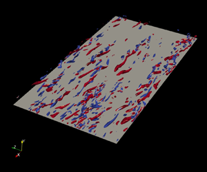
3.2.1. Identification method
In this work, vortical structures are identified by means of the  $Q$-criterion, i.e. $Q\geq Q_{thresh}$. The inhomogeneity of the channel flow is taken into account through $Q_{thresh}=Q_{thresh}(y)$ depending on the standard deviation of the second invariant of ${\mathsf{D}}_{ij}=\partial u_i/\partial x_j$, which is a more significant statistical indicator of vortical events compared with other quantities. For instance, figure 8(a) shows the mean $Q$-values normalized by their standard deviations and, as can be seen, for both GN fluid cases, in regions with $\bar {Q}>0$; i.e. regions where on average $Q$-positive values are slightly more common, $\bar {Q}\ll \textrm {rms}(Q^\prime )$. Figure 8(a) also makes apparent that, in the very near-wall region, particularly within the viscous sublayer, the mean $Q$-values are approximately of the same order of magnitude as the root-mean-squared values of its fluctuations. Other interesting observations regarding the standard deviation of the $Q$-values as a statistical indicator of vortical structures are noted by considering figure 8(b). The figure reveals an apparent inhibition of the intensity corresponding to the fluctuating $Q$-values with shear-thinning rheology. This result points to an overall decrease in the population of vortices for the drag-reducing fluid case. Figure 8(b), for both fluid cases, also displays a clear peak in the $\textrm {rms}({Q^\prime }^{+})$ profiles close to $y^+ \approx 20$ which suggests predominance of vortical structures in and close to that region of the buffer layer.

Figure 8. Low-order statistics of  $Q$-values: (a) ratio of mean $Q$-values to their standard deviations, $\bar {Q}/\textrm {rms}(Q^\prime )$, and (b) root-mean-squared fluctuating $Q$-values in inner units, $\textrm {rms}({Q^\prime }^{+})$. Line colours as explained in table 1.
According to what was discussed in the introduction and in the previous paragraph, non-zero threshold values accounting for variations in the inhomogeneous direction are to be selected in order to deliver proper results but the question about which particular threshold values should be used still remains unanswered. For instance, in the channel flow and at a given wall-normal position, a threshold value,  $\mathcal {T}$, is required to be large enough such that it is possible to distinguish individual structures and also to capture as many structures as possible. On the other hand, a too large $\mathcal {T}$-value makes it easier to identify individual structures but only captures the most intense ones. Thus, a common limitation for the $Q$-criterion and for many other identification methods, is their threshold dependency. The threshold selection remained relatively subjective until Moisy & Jiménez (Reference Moisy and Jiménez2004) introduced the percolation analysis to systematically select $\mathcal {T}$-values for proper visualization of the structures. Here, a perceptible transition from a highly clustered region to increasing individual structures, identified according to a particular method (e.g. $Q$ or $\lambda _2$-criterion), occurs at a critical threshold value, $\mathcal {T}_c$. Percolation analysis has been successfully used not only for identifying vortex clusters in turbulent channel flows (del Álamo et al. Reference del Álamo, Jiménez, Zandonade and Moser2006) but also for detecting three-dimensional velocity structures (Sillero Reference Sillero2014; Hwang & Sung Reference Hwang and Sung2018) and quadrant events in turbulent channels (Lozano-Durán, Flores & Jiménez Reference Lozano-Durán, Flores and Jiménez2012) and homogeneous shear turbulence (Dong et al. Reference Dong, Lozano-Durán, Sekimoto and Jiménez2017) based on a three-dimensional extension of the classical quadrant analysis (Wallace et al. Reference Wallace, Eckelmann and Brodkey1972; Willmarth & Lu Reference Willmarth and Lu1972). More recently, the percolation analysis for threshold selection has also been employed by Cheng et al. (Reference Cheng, Li, Lozano-Durán and Liu2020a) for the identification of scale-based structures of streamwise wall shear stress fluctuations in turbulent channel flows.
A brief description of the approach used for identifying the three-dimensional vortical structures is given as follows.
(i) For a given instantaneous flow field, the
$Q (x,y,z)$-values are computed according to (1.4).(ii) The vortical structures are identified as fluid connected regions where the criterion
(3.10a,b)is satisfied. Here, percolation analysis is used to determine the value of\begin{equation} Q (x,y,z) \ge Q_{thresh}(y);\quad Q_{thresh}(y)=\mathcal{T}\,{\text{rms}}(Q^\prime) \end{equation}$\mathcal {T}$ and the standard deviation of the $Q$-values, for cases P180 and N180, is according to the profiles presented in figure 8(b). Also, the individual structures consist of connected grid point values satisfying (3.10a,b) and connectivity is defined by the six orthogonal nearest neighbours of each grid point. Figure 9 also shows the followed procedure by means of a flowchart.


Figure 9. Flowchart of the procedure followed for the identification of three-dimensional vortical structures and computation of related statistics.
Figures 10(a) and 10(b) show the time averaged  $V_{max}/V_{tot}$; which is the ratio of the volume corresponding to the largest identified structure $V_{max}$, at a given $\mathcal {T}$, to the total volume occupied by all structures $V_{tot}$, and $N_{tot}/ N_{max}$; which is the ratio of the total number of identified objects $N_{tot}$, at a given $\mathcal {T}$, to the largest number of identified structures over all $\mathcal {T}$-values which is denoted by $N_{max}$, respectively. In the figure, for both cases, the critical threshold values; where $\textrm {d} ( V_{max}/ V_{tot})/\textrm {d} \mathcal {T}$ is a minimum and the percolation transition occurs, and the threshold value $\mathcal {T}_{max}$ where $N_{tot}= N_{max}$ are marked as well. Figure 10(a) shows that the threshold at which the merging process is more intense, i.e. $\mathcal {T}_c$, slightly decreases with shear-thinning rheology. Note that, for $\mathcal {T}< \mathcal {T}_c$ and as $\mathcal {T}$ keeps decreasing, fewer structures are identified and the existing ones keep merging until a single, large ‘sponge-like’ object remains, where $V_{tot} = V_{max}$ (del Álamo et al. Reference del Álamo, Jiménez, Zandonade and Moser2006). A tentative explanation for the decrease of $\mathcal {T}_c$ with shear-thinning behaviour may be associated with the overall decrease in the number of identified objects and the intensity of the fluctuating $Q$-values, as seen in figure 8(b) for the shear-thinning case; a cluster of objects leading to a less populated domain is likely to distinctly ‘break down’ more promptly. From figure 10(b) is also apparent that the maximum number of identified objects decreases with shear-thinning fluid behaviour; at low $\mathcal {T}$-values just a few objects are detected and the increase in the ratio $N_{tot}/ N_{max}$ with shear-thinning rheology implies that $N_{max,\textrm {P180}}< N_{max,\textrm {N180}}$. Figure 10(b) also allows us to see that $\mathcal {T}_{max}\approx 1$ for cases P180 and N180. Thus, to facilitate the comparison of the results, the threshold value in (3.10a,b) is taken equal to the value that maximizes the number of detected objects for both cases, i.e. $\mathcal {T} = \mathcal {T}_{max}$. A short discussion regarding the influence of the threshold value is presented in Appendix B.

Figure 10. Percolation diagrams: (a)  $V_{max}/ V_{tot}$ and (b) $N_{tot}/ N_{max}$. In (a and b), the line style ‘- - -’ is used to mark the critical threshold value, $\mathcal {T}_c$, and the threshold value resulting in the maximum number of objects, $\mathcal {T}_{max}$, respectively. Line colours as explained in table 1.
Finally, observations regarding the decrease in the total number of identified structures and the slight variations in their orientation (see also discussion of the ratio  $S^\star$ in § 3.1) are easily drawn as well from the isosurfaces of the instantaneous $Q$-values fulfilling (3.10a,b), which are shown in figures 11(a) and 11(b). Here, for comparison purposes, a computational box of $12h^+$ in the $x$-direction and $6h^+$ in the $z$-direction, corresponding to twice the minimal flow unit up to the logarithmic region (Flores & Jiménez Reference Flores and Jiménez2010), and centred around the midpoint in the $x-z$ plane is considered. Also, the presented objects are limited to $y^+ \lesssim 50$ and coloured by the streamwise vorticity component.

Figure 11. Isosurfaces of instantaneous  $Q (x,y,z) \geq {\text {rms}}(Q^\prime )$ coloured by streamwise vorticity, $\omega _x$, for: (a) Newtonian and (b) shear-thinning fluid cases. Blue and red colours are used to identify values of $\omega _x>0$ and $\omega _x<0$, respectively.
3.2.2. Classification: wall-attached and wall-detached structures
Each object identified with condition (3.10a,b) is circumscribed within a bounding box aligned with the Cartesian axes, which is used to define both its position and size  $l_x, l_z$ and $l_y= y_{max}-y_{min}$; where $y_{max}$ and $y_{min}$ are the maximum and minimum distances of each object to the closer wall, respectively. See figure 12. Figure 13 shows the joint probability density function (j.p.d.f.) of the minimum and maximum wall distances for the vortical structures, $p(y_{min}/h,y_{max}/h)$, for cases P180 and N180. Here, the j.p.d.f.s are approximated via joint probability mass functions (also called discrete density functions). As can be seen from figure 13, the objects can be grouped within two families based on their distance to the wall: the first family is the narrow vertical band to the left of $y_{min}/h \lesssim 20/h^+$ which includes some very tall structures reaching almost to the opposite wall, while the second family corresponds to the highly populated inclined band where $y_{min}/h > 20/h^+$, limited by $y_{max}=y_{min}$, and which structures depend little on their distance from the wall and mainly on their vertical height $l_y$. del Álamo et al. (Reference del Álamo, Jiménez, Zandonade and Moser2006) denoted the first and second families as wall-attached and wall-detached vortex clusters, respectively. Comparing figure 13(b) with 13(a) reveals that both families present taller objects with shear-thinning fluid rheology.

Figure 12. Schematic representation of an identified vortical structure circumscribed in a box of size  $l_x \times l_y \times l_z$: (a) top view and (b) side view.

Figure 13. The j.p.d.f. of the maximum and minimum wall distances of the identified structures,  $p(y_{min}/h,y_{max}/h)$: (a) N180 and (b) P180. The contours are 0.25, 0.5, 1 and $5$, from darker to lighter blue until yellow. Dashed vertical line at $y_{min}/h \lesssim 20/h^+$ and dashed horizontal line at $y_{max}/h \lesssim 50/h^+$.
For the following subsections, most of the discussion will focus on the wall-attached structures which are larger but, most importantly, interact with the near-wall flow. Also, regarding possible Reynolds number dependency of the results, it is worth pointing out that del Álamo et al. (Reference del Álamo, Jiménez, Zandonade and Moser2006) studied the vortex clusters in turbulent channels of Newtonian fluids for  $180 < Re_\tau < 1900$ and showed fairly small Reynolds number dependency in their results. Hence, we therefore anticipate that observed trends with shear-thinning fluid behaviour may hold even at higher Reynolds numbers.
3.2.3. Length scale self-similarity
Figures 14(a) and 14(b) display the p.d.f. of the aspect ratios  $l_x^+/l_y^+$ and $l_z^+/l_y^+$, respectively, for the wall-attached structures confined to the viscous wall region and for cases P180 and N180. Unsurprisingly, the peaks in the profiles showed in figures 14(a) and 14(b) suggest self-similarity of the lengths and widths of the wall-attached structures with their heights. For the Newtonian base case, $l_x^+ \approx 3 l_y^+$ and $l_z^+ \approx l_y^+$, which are similar to the linear laws reported by del Álamo et al. (Reference del Álamo, Jiménez, Zandonade and Moser2006), albeit less wide in comparison since there, $l_z^+ \approx 1.5 l_y^+$, for the tall attached structures, i.e. $y_{min}/h \lesssim 20/h^+$ and $y_{max}/h \gtrsim 100/h^+$. With respect to the shear-thinning case, $l_x^+ \approx 4.7 l_y^+$ and $l_z^+ \approx 0.9 l_y^+$. Thus, it appears that, for a given height, the structures are longer but with approximately the same width for the drag-reducing fluid rheology. With respect to the flow physics, these results show that, unlike what is observed in the streamwise direction, the character of the flow in the cross-stream planes remains unchanged with shear-thinning behaviour.

Figure 14. The p.d.f. of the bounding boxes’ aspect ratios: (a)  $l_x^+/l_y^+$ and (b) $l_z^+/l_y^+$ corresponding to the wall-attached structures, $y_{min}/h \lesssim 20/h^+$, confined to the viscous wall region, $y_{max}/h \lesssim 50/h^+$. Dashed vertical lines mark the approximate peak values of the p.d.f. Line colours as explained in table 1.
3.2.4. Scale-dependent properties
Regarding the actual shape of the identified objects, figure 15(a), displaying the j.p.d.f. of the logarithms of volumes corresponding to the wall-attached vortical structures,  $V_{core}^{+}$, and their heights, i.e. $p(\log (l_y^{+}), \log (V_{core}^{+}))$, suggests that the vortex cores grow approximately as $(l_y^{+})^{1.7}$ for both GN fluids. This result is consistent with the one reported by del Álamo et al. (Reference del Álamo, Jiménez, Zandonade and Moser2006) although, there, the power-law index is slightly larger; $V_{core}^{+}\propto (l_y^{+})^{2}$. The growth of the vortex cores contrasts with that of the circumscribing box volume, $l_x l_y l_z$, which grows as $(l_y^{+})^{3}$ for the wall-attached structures within the viscous wall region; see § 3.2.3. Thus, if the exponent found is interpreted as a fractal dimension, it implies that the identified structures are shell-like objects (del Álamo et al. Reference del Álamo, Jiménez, Zandonade and Moser2006). Figure 15(a) also reveals that the shear-thinning rheology leads to slightly larger $V_{core}^{+}$-values for a given structure height without affecting their crude estimation of their fractal dimension.

Figure 15. Scale-dependent properties: (a) j.p.d.f. of the logarithms of the volumes corresponding to the wall-attached vortical structures and their height,  $p(\log (l_y^{+}), \log (V_{core}^{+}))$, and (b) population density of the wall-attached vortical structures, $n_{s}^{+}$, as function of their wall-normal position, $y_c^{+}$. In (a), the levels represented contain 70 % and 97 % of the data, respectively, and the dashed lines, found through least-squares fitting, denote $V_{core}^{+}\approx 3.5(l_y^{+})^{1.7}$ and $V_{core}^{+}\approx 4(l_y^{+})^{1.7}$ for cases P180 and N180, respectively. Line/marker colours as explained in table 1.
Another scale-dependent property of interest is the population density defined as
 \begin{equation} n_{s}^{+}=\frac{N(y_c^{+})}{N_f L_x^{+} L_z^{+}}, \end{equation}
where  $N$ is the histogram of the wall-attached structures at a wall-normal position $y_c^{+}=y_{min}^{+} +l_y^{+}/2$. Hence, $n_{s}^{+}$ represents the number of wall-attached vortical structures per wall-normal position, number of collected flow fields and wall-normal area. Figure 15(b) displays the population density for cases P180 and N180 and consistent with the statistical indicator shown in figure 8(b), the densities peak at the buffer layer. Note that, an overall decrease in $n_{s}^{+}$, most noticeable in the buffer layer, and a slight shift towards the channel centre of the wall-normal position at which the population density peaks are also observed with shear-thinning fluid rheology. With respect to the tails of the population density profiles, although not of our main interest, it is worth mentioning that a similar decay for the population density is noticed for both cases. For the tall attached objects, $l_y^{+} \approx 2 y_c^{+}$ and $n_{s}^{+}\propto (l_y^{+})^{-3}$ (del Álamo et al. Reference del Álamo, Jiménez, Zandonade and Moser2006), which constitutes a faster decay in comparison with the wall-normal decay of the three-dimensional wall-attached quadrant events leading to positive turbulence production (Lozano-Durán et al. Reference Lozano-Durán, Flores and Jiménez2012) and the three-dimensional wall-attached structures based on intense velocity fluctuations (Cheng et al. Reference Cheng, Li, Lozano-Durán and Liu2020b). In consequence, interactions between vortical structures and other types of structures are deemed more likely to occur in regions closer to the wall.
4. Near-wall self-sustaining process
As mentioned in the introduction, a turbulent flow of a GN fluid exhibiting shear-thinning behaviour shows several features common to the LDR regime also seen in flows of polymer solutions with viscoelastic effects. Furthermore, regarding the near-wall structures and aside from the reduction in the spanwise meandering, spacing and the thickening of the velocity streaks (see e.g. Appendix A), Section 3 has provided substantial evidence about the changes of the quasi-streamwise vortices with shear-thinning behaviour; those structures seem to grow in size, depart from the wall, diminish in population and strength in a similar manner as observed when viscoelastic effects are introduced. Recall that, in viscoelastic solutions, the polymers appear to oppose the motion of the vortices (Dubief et al. Reference Dubief, Terrapon, White, Shaqfeh, Moin and Lele2005; Kim et al. Reference Kim, Li, Sureshkumar, Balachandar and Adrian2007), take energy from them and release it into the streaks through the work arising from the interactions between the corresponding fluctuating velocity and the polymer body force (Dubief et al. Reference Dubief, White, Terrapon, Shaqfeh, Moin and Lele2004, Reference Dubief, Terrapon, White, Shaqfeh, Moin and Lele2005). In the case of wall-bounded turbulent flows of a GN fluid, it is known that an analogous force arises due to fluctuations in viscosity (see e.g. Singh et al. Reference Singh, Rudman and Blackburn2017; Arosemena et al. Reference Arosemena, Andersson and Solsvik2021). To gain insight into the potential disruption in the self-sustaining cycle near the wall, in the spirit of De Angelis, Casciola & Piva (Reference De Angelis, Casciola and Piva2002), the following correlation coefficient is considered:
 \begin{equation} \text{norm}(\overline{u_i^\prime \,f_i^\prime})=\frac{\overline{u_i^\prime \,f_i^\prime}}{\text{rms}(u_i^\prime)\,\text{rms}(\,f_i^\prime)}, \end{equation}
where  $f_i^\prime$ is the fluctuating component of the new force $f_i=(1/\rho )\partial (2\mu ^\prime {\mathsf{S}}_{ij})/\partial x_j$ arising due to viscosity fluctuations. The summation convention does not apply to subscript $i$ in (4.1). The interaction term $E_i^{(NN)}=\overline {u_i^\prime \,f_i^\prime }$, appearing in the budget equation of the diagonal components of the Reynolds stress $\overline {u_i^\prime u_k^\prime }$, represents a mechanical work that can enhance $(E_i^{(NN)}>0)$ or diminish $(E_i^{(NN)}<0)$ the energy carried by the velocity component $u_i^\prime$.
Figure 16 shows  $\text {norm}(\overline {u_i^\prime \,f_i^\prime })$ confined to the viscous wall region. This correlation coefficient is an indicator of $E_i^{(NN)}$; if the correlation is positive (negative), on average, $f_i^\prime$ has the tendency to increase (decrease) $u_i^\prime$, which is equivalent to positive (negative) work. In striking contrast to viscoelastic solutions, all velocity fluctuations are, almost everywhere, enhanced by the new force $f_i^\prime$. In the case of the streamwise velocity fluctuation – related to the near-wall streaks – it is worth to note that, as for polymer solutions showing viscoelastic effects, the major enhancement occurs close to the upper edge of the viscous sublayer, i.e. $y^+\approx 5$. The wall-normal and spanwise velocity fluctuations – which in a simplified picture of near-wall turbulence are related to the quasi-streamwise vortices – are mostly enhanced by $f_y^\prime$ and $f_z^\prime$, respectively. This observation indicates that the new forces seem to support rather than to oppose the vortices and contrasts with the findings of e.g. De Angelis et al. (Reference De Angelis, Casciola and Piva2002), Dubief et al. (Reference Dubief, White, Terrapon, Shaqfeh, Moin and Lele2004), Kim et al. (Reference Kim, Li, Sureshkumar, Balachandar and Adrian2007) and Li & Graham (Reference Li and Graham2007), where it is reported that the polymer forces oppose and potentially suppress the near-wall vortices. Moreover, figure 16 also displays the profile of ${\text {norm}}(\overline {\omega _x^\prime {{MD}_{\omega _x}^{(NN)}}^\prime })$, which is the correlation coefficient between $\omega _x$ and its molecular diffusion due to viscous effects related to fluctuations in viscosity (analogous to the term interpreted as the polymer torque in Kim et al. (Reference Kim, Li, Sureshkumar, Balachandar and Adrian2007) when considering viscoelastic effects); as seen from the figure, since outside the viscous sublayer the correlation is positive, the effects due to viscosity fluctuations appear to neither act in opposition to the streamwise vorticity component nor reduce the strength of the near-wall quasi-streamwise vortices.

Figure 16. Correlation coefficients potentially related to disruption in the near-wall self-sustaining cycle for the viscous wall region,  $y^{+} \leq 50$. Profiles corresponding to correlation coefficients of $\overline {u^\prime f_x^\prime }$, $\overline {v^\prime f_y^\prime }$, $\overline {w^\prime f_z^\prime }$ and $\overline {\omega _x^\prime {{MD}_{\omega _x}^{(NN)}}^\prime }$ are indicated by the line styles ‘—–’, ‘- - -’, ‘ $\cdot \cdot \cdot$’ and ‘- $\cdot$ -’, respectively. Line colours as explained in table 1.
Finally, although the forces arising due to viscosity fluctuations appear to enhance the different turbulent intensities, it is important to consider these effects in conjunction with those resulting from the local increase of mean viscosity with shear-thinning behaviour. Figure 17(a–c) presents the total contribution to the budgets of  $\overline {u^\prime u^\prime }$, $\overline {v^\prime v^\prime }$ and $\overline {w^\prime w^\prime }$ attributed to viscous effects related to the mean viscosity and its fluctuations, i.e. $2 E_i^{(N)}$ and $2 E_i^{(NN)}$, respectively. Here, the interaction term $E_i^{(N)}=\overline {u_i^\prime g_i^\prime }$, $g_i^\prime = (1/\rho )\partial (2\bar {\mu }{\mathsf{S}}_{ij}^\prime )/\partial x_j$; summation is applied over index $j$ but not over index $i$. As expected, for the shear-thinning fluid, contributions due to fluctuations in viscosity are fairly small in comparison with those due to the mean viscosity; see the terms related to the budgets of $\overline {v^\prime v^\prime }$ and $\overline {w^\prime w^\prime }$. Nonetheless, as displayed in figure 17(a), $2 E_x^{(NN)}$ appears to be a source term to the $\overline {u^\prime u^\prime }$-budget that cannot be neglected. An intriguing situation when considering the budget of $\overline {u^\prime u^\prime }$ for a shear-thinning fluid in comparison with a Newtonian base case (see e.g. Arosemena et al. Reference Arosemena, Andersson and Solsvik2021), is that, although the production term is decreasing due to the decrease in Reynolds shear stress with shear-thinning behaviour (see figure 1b), there is an increase in the streamwise turbulence intensity as reported by several authors (see e.g. Gavrilov & Rudyak Reference Gavrilov and Rudyak2016; Singh et al. Reference Singh, Rudman and Blackburn2017; Arosemena et al. Reference Arosemena, Andersson and Solsvik2021). In consequence, the interpretation of $2 E_x^{(NN)}$ as an additional source term to the $\overline {u^\prime u^\prime }$-budget, explains this well-known observation. The increase in $|2 E_x^{(N)}|$ observed in figure 17(a) with shear-thinning rheology, required to balance out the overall budget, is also attributed to this new source term. Thus, based on these observations, it is really not surprising that the streaks are thickened and display less meandering/streakiness with shear-thinning behaviour. On the other hand, consistent with the decrease in energy redistribution from the $\overline {u^\prime u^\prime }$-budget through the velocity–pressure gradient term with shear-thinning behaviour (Arosemena et al. Reference Arosemena, Andersson and Solsvik2021), there is a decrease in $|2 E_y^{(N)}|$ and $|2 E_z^{(N)}|$ observed in figures 17(b) and 17(c), respectively. The fact that less energy is available for the cross-sectional intensities is certainly related to the observed suppression of the quasi-streamwise vortices with shear-thinning rheology.

Figure 17. Contributions due to viscous effects, for  $y^{+} \leq 50$, to the budgets of: (a) $\overline {u^\prime u^\prime }$, (b) $\overline {v^\prime v^\prime }$ and (c) $\overline {w^\prime w^\prime }$. Profiles corresponding to total contributions due to the mean viscosity, $2{E_i^{(N)}}^{+}$, and its fluctuations, $2{E_i^{(NN)}}^{+}$, are indicated by the line styles ‘—–’ and ‘- - -’, respectively. Line colours as explained in table 1.
It is also worth pointing out that the results of this section are in line with our previous remark about the character of the flow which, unlike the streamwise direction, seems to be unaffected in the cross-stream planes with shear-thinning fluid behaviour; see § 3.2.3. In summary, despite the similar flow characteristics between drag-reducing viscoelastic flows and those of (purely viscous) shear-thinning behaviour, the disruption of the near-wall self-sustaining process does not seem to occur in the same manner. The features of Newtonian near-wall structures remain also for the shear-thinning case; the near-wall vortices cause the streaks and, for instance, their instability or local regions of longitudinal vorticity, that may roll-up, form the coherent quasi-streamwise vortices. The difference is that with shear-thinning rheology, the viscosity – a function of the local properties of the flow – increases as we move away from the wall and a new force arises due to viscosity fluctuations. These two factors appear to be leading to less energetic streamwise-oriented vortical motions and more stable and thicker streaks, respectively.
5. Conclusions
Data of statistically converged turbulent channel flow simulations of GN fluids at  $Re_\tau = 180$ (Arosemena et al. Reference Arosemena, Andersson and Solsvik2021) are considered to analyse how the near-wall quasi-streamwise vortices change with shear-thinning rheology compared with the Newtonian base case. The shear-dependent rheology leads to drag reduction amounting to approximately $10\,\%$ and the study comprises statistics compiled from flow field variables and from identified three-dimensional vortical structures. The following can be inferred from the flow statistics:
(i) On average (in time and in the homogeneous spatial directions), compared with the Newtonian fluid case, the quasi-streamwise vortices appear to grow in size, depart from the wall and decrease in intensity with shear-thinning rheology. In particular, it is found that the different terms involved in production of streamwise vorticity,
$P_{\omega _x}$, are suppressed with shear-thinning fluid behaviour.(ii) Also, with respect to the near-wall small-scale motions and the vorticity field, outside the viscous sublayer, an increase in the time scale of vorticity relative to that of the mean shear,
$S^\star$, is noticed for the shear-thinning rheology. Such increase in $S^\star$ suggests that the vortical structures will tend to be slightly more oriented along the most extensive strain direction of the mean flow and also pushes the small-scale eddies towards higher anisotropy states.


Furthermore, considering the identified vortical structures, we reported the following findings:
(i) Tall attached and detached families (del Álamo et al. Reference del Álamo, Jiménez, Zandonade and Moser2006) are also observed with shear-thinning rheology, however, both families appear to be comprised by taller objects in comparison with the Newtonian fluid case.
(ii) Regarding the geometry of the structures confined to the viscous wall region, when they are inscribed into parallelepipedal boxes aligned with the Cartesian axes, the boxes are self-similar, with dimensions
$l_x^+ \approx 3 l_y^+$, $l_z^+ \approx l_y^+$ and $l_x^+ \approx 4.7 l_y^+$, $l_z^+ \approx 0.9 l_y^+$ for the Newtonian and shear-thinning fluid cases, respectively. Hence, the vortical structures of a particular height appear to be more elongated but with approximately the same width for the drag-reducing fluid case. This shows that, unlike what is observed in the streamwise direction, the character of the flow in the cross-stream planes remains unchanged with the shear-thinning rheology.(iii) Also, related to the geometry of the structures, it is found that the actual shape of the vortex cores is still shell like for the shear-thinning fluid case; although, shear-thinning rheology leads to larger volumes, for a given circumscribing box height, their fractal dimension remains the same.
(iv) Finally, a decrease in the population density is observed with the shear-dependent rheology and its peak, at the buffer layer, is significantly suppressed and seen slightly shifted away from the wall. This observation is consistent with the previous remark, inferred from the flow statistics, about the departure of longitudinal vortices from the vicinity of the wall for the drag-reducing fluid case.


The above findings, by themselves, are useful for the study of certain topics in different fields, for instance, in chemical engineering, information about the aspect ratio and number density of the turbulent vortices are of practical importance when computing the rate of interaction between continuous and dispersed phase in the closure models for fluid particle breakup and coalescence due to turbulence (see e.g. Ghasempour et al. Reference Ghasempour, Andersson, Andersson and Bergstrom2014; Solsvik & Jakobsen Reference Solsvik and Jakobsen2016). Furthermore, these results – in conjunction with the observed changes on the near-wall velocity streaks due to the shear-thinning rheology (see e.g. Appendix A) – strongly suggest that the self-sustaining process in the vicinity of the wall has been disrupted.
The study of the interaction between velocity fluctuations and forces related to the viscous effects revealed that, despite the phenomenological similarities with other LDR regime flows, such as those with viscoelastic effects, the qualitative features of the Newtonian near-wall structure remain for the shear-thinning case; quasi-streamwise vortices cause the velocity streaks and either their instability or other parent vortices produce the near-wall rolls. The difference with the shear-thinning rheology is the local increase of viscosity – experienced as we move away from the wall – which seems to lead to less energetic vortices, whereas the streaks are provided with an additional source of energy due to fluctuations in viscosity.
Acknowledgements
The authors are grateful for computer resources provided by NTNU IDUN/EPIC computing cluster (Själander et al. Reference Själander, Jahre, Tufte and Reissmann2019).
Funding
This work was supported by the Research Council of Norway (RCN, grant no. 274398).
Declaration of interests
The authors report no conflict of interest.
Appendix A. Effects on the velocity structures
In the shear-dominated viscous and buffer layers, the velocity structures consist of an irregular array of spanwise staggered, alternating regions of low- and high-speed fluid elongated in the streamwise direction and superimposed to the mean flow. In a canonical flow, such as a fully developed channel or a boundary layer of a Newtonian fluid, the streaks are quite long (streamwise length  $\lambda _x^+ \approx 10^3\text {--}10^4$) with an average spanwise spacing $\lambda _z^+ \approx 100$ (Smith & Metzler Reference Smith and Metzler1983).
Information about the effects on the near-wall velocity structures due to shear-thinning rheology can be obtained by analysing the two-point correlation  ${\mathsf{R}}_{11}$ for separations in the longitudinal and lateral directions. As seen in figure 18(a), ${\mathsf{R}}_{11}(\delta x^+)$ decays more slowly with increasing $\delta x^+$ for the shear-thinning fluid than for the Newtonian fluid; indicating that the streaks are coherent over longer streamwise distances. This is more noticeable as the distance from the wall decreases, see the contours of instantaneous ${u^\prime }^+$ at the same wall-normal positions in figure 19. Note that for comparison purposes, and since the computational domain for P180 is larger than for case N180, the bounding box for both GN fluid cases has been set to $12h^+$ in the $x$-direction and to $6h^+$ in the $z$-direction centred around the midpoint in the $x\text{-}z$ plane. This box constitutes twice the box size containing the minimal flow unit in the logarithmic layer, as discussed by Flores & Jiménez (Reference Flores and Jiménez2010) and thus, it is considered more than enough to observe several streaks within the viscous wall region even for the shear-thinning fluid case.

Figure 18. Normalized two-point correlation  ${\mathsf{R}}_{11}$ with: (a) streamwise separation, $\delta x^+$, and (b) spanwise separation, $\delta z^+$. Line styles ‘—–’, ‘- - -’ and ‘ $\cdot \cdot \cdot$’ are used to identify correlations at $y^+ \approx 5, 30$ and 50, respectively. Line colours as explained in table 1.

Figure 19. Contours of instantaneous streamwise velocity fluctuations normalized by frictional velocity for Newtonian (left panels) and shear-thinning (right panels) fluid cases at: (a,b)  $y^+ \approx 5$, (c,d) $y^+ \approx 30$ and (e,f) $y^+ \approx 50$. White and blue represent negative and positive fluctuations, respectively.
Figure 18(b), on the other hand, shows  ${\mathsf{R}}_{11}(\delta z^+)$ decaying rapidly and, at a given $y^+$, attaining a minimum at a larger spanwise separation with shear-thinning rheology. The location of this minimum is the average distance between a high- and a low-speed streaks and, in consequence, the average streak spacing $\lambda _z^+$ is twice such distance (Moser & Moin Reference Moser and Moin1984). Figure 20 shows the average streak spacing for both cases and a distinct increase in $\lambda _z^+$ is observed with shear-thinning fluid behaviour. Note that, at $y^+ \approx 5\text {--}10$, the attained streak spacing is close to the predicted value based on the expression proposed by Oldaker & Tiederman (Reference Oldaker and Tiederman1977) for wall-bounded flow of a polymer solution. Also, as for a Newtonian fluid, $\lambda _z^+$ increases with increasing distance from the wall. An interesting observation regarding the streak spacing, in the region close to the viscous sublayer, is that its increase is accompanied by an increase in the average lifetime of a streak which is less or equal to the time interval between bursts (Achia & Thompson Reference Achia and Thompson1977). The meaning of ‘bursting’ varies between authors but here it is used to describe the three-stage process of low-speed streak lift-up, oscillation and breakup (Kim, Kline & Reynolds Reference Kim, Kline and Reynolds1971). The increase in the lifetime of a sublayer streak suggests an increase in their stability with shear-thinning rheology and in consequence, less bursting and overall lessening of the turbulent generating events (see for instance the quadrant analysis of Arosemena et al. Reference Arosemena, Andersson and Solsvik2021).

Figure 20. Average spanwise spacing between streaks,  $\lambda _z^+$. Line style ‘—–’ corresponds to correlation $\lambda _z^+ = 1.9 \mathrm {DR} \%+99.7$ proposed by Oldaker & Tiederman (Reference Oldaker and Tiederman1977) for region close to the viscous sublayer. Marker colours as explained in table 1.
Another important quantity when considering how the energy-containing motions are affected with shear-thinning rheology in a turbulent shear flow, is the turbulent-to-mean-shear time scale ratio (Corrsin Reference Corrsin1957) given by
 \begin{equation} S^* = \frac{2\bar{{\mathsf{S}}}_{12}k}{\epsilon_k}, \end{equation}
where  $2\bar {{\mathsf{S}}}_{12} = \partial \bar {u}/\partial y$ is the shear rate, $k=\overline {u_i^\prime u_i^\prime }/2$ is the turbulent kinetic energy and $\epsilon _k$ is the total mean dissipation rate in the GN fluid flow. Hence, the shear parameter $S^*$ represents a dimensionless measure of the interaction between the mean shear and the large-scale energy-containing, eddies (Jiménez Reference Jiménez2013). The shear parameter is presented in figure 21(a). Within the viscous wall region, for both fluid cases, it is clear that $S^* \gg 1$ and many similarities – in the instantaneous structures and turbulent statistics – with homogeneous shear flow at comparable $S^*$ values and thus with linearized rapid-distortion theory (Lee et al. Reference Lee, Kim and Moin1990) are expected. Also, with shear-thinning rheology and for $y^+ <50$, the increase in the ratio of energy-decay time to the time scale of mean deformation implies an increase in the amount that turbulent kinetic energy production exceeds total dissipation. Such increase in $S^*$ for the shear-thinning fluid case implies as well that, compared with the Newtonian base case, mean shear dominates even more the large-scale motions.

Figure 21. Mean-shear-related properties of the energy-containing scales: (a) turbulent-to-mean-shear time scale ratio,  $S^*$, vs $y^+$ and (b) $S^*$ vs second invariant of the Reynolds stress anisotropy tensor, $3\eta _{b}$. Line colours as explained in table 1.
A straightforward way to quantify the effect over the energy-containing scales, is to measure their anisotropy. A convenient indicator of turbulence anisotropy at large scales is the variable  $\eta _b = ({\mathsf{b}}_{ij} {\mathsf{b}}_{ji} /6)^{1/2}$, see for instance Choi & Lumley (Reference Choi and Lumley2001), which is based on the second invariant of the Reynolds stress anisotropy tensor (Lumley & Newman Reference Lumley and Newman1977) defined as
 \begin{equation} {\mathsf{b}}_{ij}=\frac{\overline{u_i^\prime u_j^\prime}}{\overline{u_k^\prime u_k^\prime}} - \frac{1}{3} \delta_{ij}. \end{equation}
Figure 21(b) shows  $S^*$ against $3\eta _b$. The variable $3\eta _b$ varies from unity for velocities completely aligned in one direction to zero for fully isotropic ones. As can be seen, the increase in the shear parameter with shear-thinning rheology is accompanied by an overall increase in large-scale anisotropy, which is consistent with the reported enhancement of streamwise turbulence intensity and the inhibition of the other cross-sectional intensities by multiple authors (see, e.g. Gavrilov & Rudyak Reference Gavrilov and Rudyak2016; Singh et al. Reference Singh, Rudman and Blackburn2017; Arosemena et al. Reference Arosemena, Andersson and Solsvik2021). Furthermore, figure 21(b) clearly shows that in the buffer layer, at a $y^+$ value close to $10$, the increase in the maximum value for the shear parameter from $S^*_{max} \approx 19$ to $S^*_{max} \approx 28$ with non-Newtonian rheology pushes the energy-containing eddies towards a one-component turbulent state similar to what it is obtained in the limit when initially isotropic turbulence goes through a hypothetical slip-free asymmetric diffuser (Hanjalić & Launder Reference Hanjalić and Launder2011).
Appendix B. The influence of the selected threshold, $\mathcal {T}$

The influence of the threshold value, in the range  $\mathcal {T}_c \leq \mathcal {T} \leq 3\mathcal {T}_c$, is considered. Figures 22(a) and 22(b) present the p.d.f. of the bounding boxes’ aspect ratios and allow us to notice an increase in their peak values and a slight shift towards lower aspect ratios with increasing threshold, $\mathcal {T}$, values. However, the overall shape of the distributions and the trend of longer bounding boxes of about the same width, for the shear-thinning case in comparison with the Newtonian one, persists. Note that, in (3.10a,b), $\mathcal {T}$ is set to $\mathcal {T}_{max}\approx 1$ and thus, $\mathcal {T}\approx 1.67 \mathcal {T}_c$ and $\mathcal {T}\approx 1.85 \mathcal {T}_c$ for the Newtonian and shear-thinning cases, respectively. In consequence, a slight decrease in the overall number of structures is expected for $\mathcal {T}= 2 \mathcal {T}_c$ and $\mathcal {T} = 3 \mathcal {T}_c$; this explains the increase in the peaks of the probability distributions with increasing $\mathcal {T}$-values.

Figure 22. The p.d.f. of the bounding boxes’ aspect ratios: (a)  $l_x^+/l_y^+$ and (b) $l_z^+/l_y^+$ corresponding to the wall-attached structures, $y_{min}/h \lesssim 20/h^+$, confined to the viscous wall region, $y_{max}/h \lesssim 50/h^+$. The line styles ‘—–’, ‘- - -’ and ‘ $\cdot \cdot \cdot$’ are used to identify the threshold values $\mathcal {T}= \mathcal {T}_c$, $\mathcal {T}= 2 \mathcal {T}_c$ and $\mathcal {T}= 3 \mathcal {T}_c$, respectively. Line colours as explained in table 1.
Figure 23 displays the effect of the threshold  $\mathcal {T}$ on the crude estimate of the fractal dimension of the vortex cores, $\beta$; $V_{core}^{+}\propto (l_y^{+})^{\beta }$. As seen from this figure, $\beta$ remains close to $1.7$ for both cases and for the considered range of $\mathcal {T}$-values.

Figure 23. Crude estimate of the fractal dimension of the vortex cores,  $\beta$, as a function of $\mathcal {T}/\mathcal {T}_c$. Marker colours as explained in table 1.


 Open access